How Important is Human Capital?

A Quantitative Theory Assessment

of World Income Inequality ∗

Andres ErosaUniversity of Toronto

Tatyana KoreshkovaConcordia University

Diego RestucciaUniversity of Toronto

February 2007

Abstract

We develop a quantitative theory of human capital investment in order to evaluatethe magnitude of cross-country differences in total factor productivity (TFP) that ex-plains the variation in per-capita incomes across countries. We build a heterogeneous-agent economy with cross-sectional variation in ability, schooling, and expenditures onschooling quality. In our theory, the parameters governing human capital productionand random ability process have important implications for a set of cross-sectionalstatistics − Mincer return, variance of earnings, variance of schooling, and intergenera-tional correlation of earnings. These restrictions of the theory and U.S. household dataare used to pin down the key parameters driving the quantitative implications of thetheory. Our main finding is that human capital accumulation strongly amplifies TFPdifferences across countries. In particular, we find an elasticity of output per workerwith respect to TFP of 2.8: a 3-fold difference in TFP explains a 20-fold differencein output per worker. We argue that the cross-country differences in human capitalimplied by the theory are consistent with a wide array of evidence including earningsof immigrants in the United States, average mincer returns across countries, and therelationship between average years of schooling and per-capita income across countries.The theory implies that using Mincer returns to measure human capital understatesdifferences across countries by a factor of 2.

Keywords : output per worker, TFP, human capital, heterogeneity, inequality.JEL Classification: O1.

∗The authors would like to thank seminar and workshop participants at Queens University, Arizona StateUniversity, ASU Development Workshop, HEC Montreal, University of Montreal, Federal Reserve Bankof Richmond, 2006 NBER Summer Institute Growth Workshop, McGill University, University of Texas-Austin, University of Southern California, Bank of Canada Productivity Workshop, Concordia University,Carleton University, University of Tokyo and Seoul National University. The paper has previously circu-lated under the title “On the Aggregate and Distributional Implications of Productivity Differences AcrossCountries.” Contact Information: Department of Economics, University of Toronto, 150 St. George Street,Toronto, Ontario M5S3G7, Canada. E-mail: andres.erosa@utoronto.ca; tkoreshk@alcor.concordia.ca; anddiego.restuccia@utoronto.ca.

1 Introduction

One of the most important challenges faced by economists is to explain the observed large

differences in per capita income across countries. In this paper we develop a quantitative

theory of human capital investments in order to evaluate the magnitude of cross-country

differences in the total factor productivity (TFP) that explains the variation in per capita

income across countries. Building a quantitative theory allows us to circumvent two major

problems faced by growth accounting exercises. First, to date, there are no reliable cross-

country measures of the quality of schooling across countries. If this quality is positively

associated with the level of economic development, the residual in growth accounting ex-

ercises overstates the cross-country differences in TFP. A second problem arises due to the

(unobserved) covariance of TFP with measures of physical and human capital, which renders

output variance decomposition difficult.

Our approach consists of developing a theory of human capital investments − schooling

time and expenditures on schooling quality − that can be used to quantitatively assess the

sources of cross-country income differences. We show that the quantitative implications of

human capital theory hinge crucially on the value of the elasticity of human capital with

respect to the expenditure on goods.1 The intuition is simple: If schooling requires only time

inputs, a change in the wage rate affects equally the benefits and the costs of human capital

accumulation, leaving the optimal level of human capital unchanged. On the contrary, when

schooling requires only inputs of goods, an increase in the wage rate raises benefits but not

the costs of schooling, hence increasing the optimal human capital stock. Therefore, the

relative importance of time versus goods inputs determines the responsiveness of human

capital to differences in the wage rate or TFP.2

1Trostel (1993) and Erosa and Koreshkova (forthcoming) make a similar point when studying the taxationof income.

2Bils and Klenow (2000) point out that the production of human capital is more intensive in time inputsthan the production of output goods. They and Klenow and Rodriguez-Clare (1997) argue that, by using aone-sector growth model, Mankiw, Romer, and Weil (1992) overstate the importance of goods inputs in theproduction of human capital and, thus, obtain results that understate TFP differences across countries.

1

Developing a quantitative theory, in turn, is a challenging task due to the lack of con-

clusive micro evidence on the expenditure elasticity of human capital: some key human

capital determinants, such as individual ability and private expenditures on education (in-

cluding those outside of formal schooling), are not observed. We address this problem by

building a theory of heterogeneous agents with cross-sectional variation in ability, school-

ing, and expenditures on schooling quality. In our theory, the parameters governing the

human capital technology and random ability process have important implications for a set

of cross-sectional statistics − Mincer return, variance of earnings, variance of schooling, and

intergenerational correlation of earnings − estimates of which are actually available in the

data. Thus we use the restrictions of the theory and U.S. household data to pin down the

key parameters driving the quantitative implications of the theory. We then use the theory

to study income inequality across countries and, in particular, to quantitatively assess how

variations in TFP are amplified through human capital accumulation into larger differences

in output per worker across countries.

Our main finding is that human capital accumulation strongly amplifies TFP differences

across countries: under the benchmark calibration, the elasticity of output per worker with

respect to TFP is 2.8. This implies that a 3-fold difference in TFP explains a 20-fold

difference in the output per worker, observed between the 10 percent richest and 10 percent

poorest countries in the world. In contrast, without human capital accumulation, the same

difference in TFP generates only a 5-fold difference in output per worker, with physical

capital being the sole source of amplification. Moreover, the theory implies that using Mincer

returns to measure human capital stocks − as typically done in growth accounting exercises

− understates differences in human capital across rich and poor countries by a factor of 2.

This occurs because Mincer returns do not capture differences in schooling quality across

countries, which our theory finds to be quantitatively important.

To evaluate the robustness of our quantitative theory, we perform a sensitivity analysis.

While the calibration of our model involves solving a multi-dimensional mapping from pa-

2

rameters to targets, the target for the share of time inputs in expenditures on human capital

has a first-order effect on the goods elasticity of human capital (and hence, on the TFP elas-

ticity of output per worker). In our baseline calibration, we use an estimate from Kendrick

(1976) and the U.S. Department of Education (1996) to set the target for the time share

at 90 percent.3 Since this target plays such a crucial role in our results and its accurate

estimate is difficult to obtain, we recalibrate the model economy by targeting alternative

values for the time share: 100, 95, 90, and 85 percent. We find that the TFP elasticity of

output per worker varies substantially across the calibrated economies: from 1.49 for the

time share of 100 percent to 3.6 for the time share of 85 percent. These figures conceal a

dramatic variation in the amplification effect of TFP: a 3-fold difference in TFP translates

into a variation in output per worker that ranges from 5-fold (time share 100 percent) to a

54-fold difference (time share 85 percent). Given the high sensitivity of results, we confront

the predictions of the calibrated models with cross-country data. To this end, for each of the

specifications, we generate artificial cross-country data by simulating economies that vary in

their relative levels of TFP.

Our baseline model economy successfully replicates the cross-country variation in school-

ing and Mincer returns (and so does the economy with a time share of 85 percent). On

the contrary, the model with only time inputs generates neither schooling nor Mincer return

variation across countries − an implication that is grossly at odds with the data. More-

over, the absence of goods in our human capital theory means no cross-country differences

in schooling quality and hence in human capital, which contradicts the empirical findings of

Borjas (1987) and Hendricks (2002) on immigrant earnings in the United States. In partic-

ular, Borjas estimates the elasticity of schooling quality with respect to the home-country

per capita income to be 0.12. In our model economies, this elasticity ranges from 0.07 (time

share 95 percent) to 0.16 (time share 85 percent), with our baseline calibration delivering

3While this observation motivates Bils and Klenow (2000) to abstract from modeling investment of goodsaltogether in human capital accumulation, our findings indicate that even a small 10 percent share of goodsin human-capital expenditures generates a large amplification effect of TFP differences across countries.

3

0.10, the closest value to the Borjas’ estimate. Furthermore, among the alternatives, the

baseline calibration provides the most consistent account of Hendricks’ evidence on immi-

grant earnings. Therefore, we conclude that the cross-country data supports a time-share

target close to 90 percent, as is the case in our baseline calibration, and an associated TFP

elasticity of output per worker of 2.8.

The paper proceeds as follows. The next section describes in detail the economic envi-

ronment. In section 3, we consider a version of the model economy with complete markets

to show how the quantitative implications of the theory for income inequality -within and

across countries- depend crucially on the expenditure elasticity of human capital. We also

derive some valuable insights that help us motivate our calibration strategy. Section 4 lays

out the calibration of the benchmark economy and discusses some properties of this economy.

In section 5, we evaluate the aggregate impact of TFP differences across countries, perform

a sensitivity analysis, and compare our findings to related papers in the literature. Section

6 concludes.

2 Economic environment

We consider an economy populated by overlapping generations of people who are altruistic

toward their descendants. People are heterogeneous in skills and physical assets and face

idiosyncratic (uninsurable) uncertainty about their labor earnings. Investment in human

capital involves the investment of children’s time and expenditures by parents that affect the

quality of the human capital of their children. Parents cannot borrow to finance investment

in human capital. Since the analysis in this paper focuses on steady states, time subscripts

are omitted in the description of the model and use a prime to indicate the next period value

of a given variable.

Demographic structure There is a large number of dynasties (mass one). The economy

is populated by overlapping generations of people who live for 5 periods and are altruistic

4

toward their descendants. The model period is set to 16 years. People live three periods

as adults and two periods as children. Panel A of Table 1 summarizes the demographic

structure in the model and the mapping between age in the model and real age in the data.

In order to match individual life expectancy in the model to that observed in the United

States, we introduce an exogenous probability of survival from period 4 to period 5, φ. A

household is composed of a parent-child pair in the first two stages and a retired adult in

the last stage. These three stages of the life cycle of households are described in Panel B of

Table 1.

Table 1: Demographic Structure and Life-cycle Stages of Households

Panel A: Demographic Structure

Model Age Real Age Name1 6-21 child2 22-37 old child3 38-53 young adult4 54-69 old adult5 70-85 retired adult

Panel B: Life-cycle Stages of Households

Stage Adult Adult’s Age Child Child’s Age1 young 38-53 child 6-212 old 54-69 old child 22-373 retired 70-85 − −

Production technologies Output is produced with a constant returns to scale technology,

Y = AKαH1−α, 0 < α < 1, (1)

where Y denotes output, K represents physical capital services, H stands for aggregate

human capital services, and A is total factor productivity (TFP). Output can be consumed

5

C, invested in physical capital X, and invested in human capital E. Feasibility requires

C +X + E = Y . Physical capital is accumulated according to

K ′ = (1− δ)K + AkX, Ak ≤ 1,

where Ak is a parameter determining the productivity of investment in physical capital (i.e.,

the effectiveness with which current period output can be transformed into capital available

for production in the following period). The aggregate human capital H is given by the

sum of human capital services in the production of goods. Human capital of an individual is

produced with the inputs of time (s) and expenditures in human capital quality (e) according

to the following production function:

h′ = z′(sηe1−η

)ξη, ξ ∈ (0, 1),

where z′ is a stochastic earnings (or learning) ability. Individuals are ex-ante identical in

their endowment of time but ex-post heterogeneous in their earnings ability. A unit of

schooling time (quantity of schooling) is produced with one unit of child’s time (s), and l

units of market human capital services. In other words, schooling requires own time and

time purchased in the market. Earnings ability is transmitted across generations according

to a discrete Markov transition matrix Q(z, z′), where qi,j = Pr(z′ = zi|z = zj). We abstract

from on-the-job human capital accumulation. In order to capture a realistic life-cycle profile

of wages, we instead assume an exogenous path of life-cycle productivity (ψc, ψy, ψo) for

children, young adults, and old adults. The productivity of old children is normalized to

one. Our abstraction is motivated by tractability reasons as well as some empirical evidence

across countries. Using the coefficients for returns to experience for each country reported in

Bils and Klenow (2000), we found that the earnings of a worker with 20 years of experience

relative to a worker with 10 years of experience is not systematically related to the level of

per-capita income across countries. In fact, we found a small negative correlation between

6

returns to labor market experience (wage growth) and per-capita income across countries,

which suggests that on the job investments in human capital are not likely to be an important

source of income differences across countries.

Market structure We assume competitive markets for factor inputs and outputs. Firms

take factor prices as given and maximize profits by choosing the demand for factor inputs:

maxK,H>0

{AKαH1−α − wH − (r + δ)K

}. (2)

Public Education Since our calibration strategy is to use cross-sectional heterogeneity

within a country to restrict the parameters governing human capital accumulation, we cannot

abstract from the role of public education on education and labor market outcomes. We

model public education by assuming that education expenditures are subsidized at the rate

p per unit of schooling time. These expenditures are financed with a proportional tax

τ on household’s income. Public and private expenditures are perfect substitutes in the

production of human capital.

Decision problem of the household All decisions of the household are made by the

parent. We assume that markets are imperfect in that households cannot perfectly insure

against labor-market risk and they cannot borrow. The state of a young parent is given by a

triple (z, h, q): earnings ability z, human capital h, and parental transfer q received from the

previous household in the dynasty line. Households maximize discounted lifetime utility of

all future generations in the dynasty. Young parents choose consumption cy, assets a′y, time

spent in school by their children s (where 1−s is working time of the children), and resources

spent on the quality of education of their children e. A parent who provides his child with s

years of schooling and a quality of education e incurs expenditures of e+(wl−p)s, where wl

is a cost per year of education (which is assumed to depend on the market wage rate) and p

denotes public education expenditures (or subsidies) per year of education. We take a broad

7

view of human capital and interpret the quality of education e as including non-education

expenditures (such as child-rearing and health care) that enhance future earnings of children.

Young parents face uncertainty regarding the ability of their children z′ which is realized in

the second stage of the household’s life cycle.

In the second stage, the household consists of a child with earnings wh′ and a parent

with earnings ψowh. Old parents decide savings for retirement a′o, consumption co, and an

intergenerational transfer q′ for the next household in the dynasty. Retired people consume

their savings.

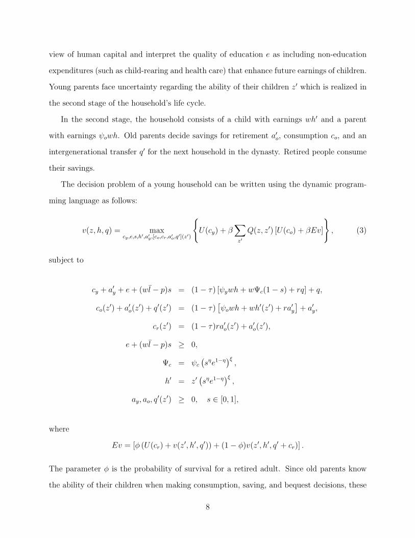
The decision problem of a young household can be written using the dynamic program-

ming language as follows:

v(z, h, q) = maxcy ,e,s,h′,a′y ,[co,cr,a′o,q′](z′)

{U(cy) + β

∑z′

Q(z, z′) [U(co) + βEv]

}, (3)

subject to

cy + a′y + e+ (wl − p)s = (1− τ) [ψywh+ wΨc(1− s) + rq] + q,

co(z′) + a′o(z

′) + q′(z′) = (1− τ)[ψowh+ wh′(z′) + ra′y

]+ a′y,

cr(z′) = (1− τ)ra′o(z

′) + a′o(z′),

e+ (wl − p)s ≥ 0,

Ψc = ψc

(sηe1−η

)ξ,

h′ = z′(sηe1−η

)ξ,

ay, ao, q′(z′) ≥ 0, s ∈ [0, 1],

where

Ev = [φ (U(cr) + v(z′, h′, q′)) + (1− φ)v(z′, h′, q′ + cr)] .

The parameter φ is the probability of survival for a retired adult. Since old parents know

the ability of their children when making consumption, saving, and bequest decisions, these

8

choices are expressed as contingent on their children’s ability z′ in the dynamic programming

problem of young parents.

3 Human capital investments in a complete markets

environment

This section provides some analytical results that shed light on how the parameters of the

human capital technology determine the quantitative implications of the theory. To this end,

we study two simplified versions of the model economy. In both specifications we assume

complete markets so that human capital investment decisions are independent of consump-

tion decisions. The first specification assumes a deterministic ability so that dynasties face no

uncertainty. We show that the parameters of the human capital technology that determine

earnings inequality in the economy (across individuals with different ability) also determine

the income inequality across countries (with different TFP). In particular, the quantitative

implications of the theory for income inequality − within and across countries − depend

crucially on the expenditure elasticity of human capital. We then show that our results ex-

tend to the complete markets economy with stochastic ability. Moreover, the cross-sectional

implications of the complete market economy provide valuable insights for calibrating the

benchmark economy with incomplete markets and for understanding the quantitative find-

ings of the paper.

3.1 Deterministic ability

Consider a world with a large number of countries. Each country is populated by measure

1 of dynasties and is characterized by a fixed TFP level A, which varies across countries

according to a cdf GA with a continuous density function. Each dynasty is characterized by

a fixed ability level, which varies across dynasties according to a cdf Gz with a continuous

density function. Denote the variance of lnA and of ln z by σ2A and σ2

z .

9

Capital markets are assumed to be perfect so that in equilibrium individuals make efficient

investments in human capital. The attention is confined to the steady state analysis. The

equilibrium interest rate is given by the individuals rate of time preference ρ ≡ 1/β − 1.

Although the theory makes no predictions for the distribution of income, consumption, and

wealth, it does have important implications for the variation of schooling and earnings −

across individuals and countries − and for the variation of output across countries.

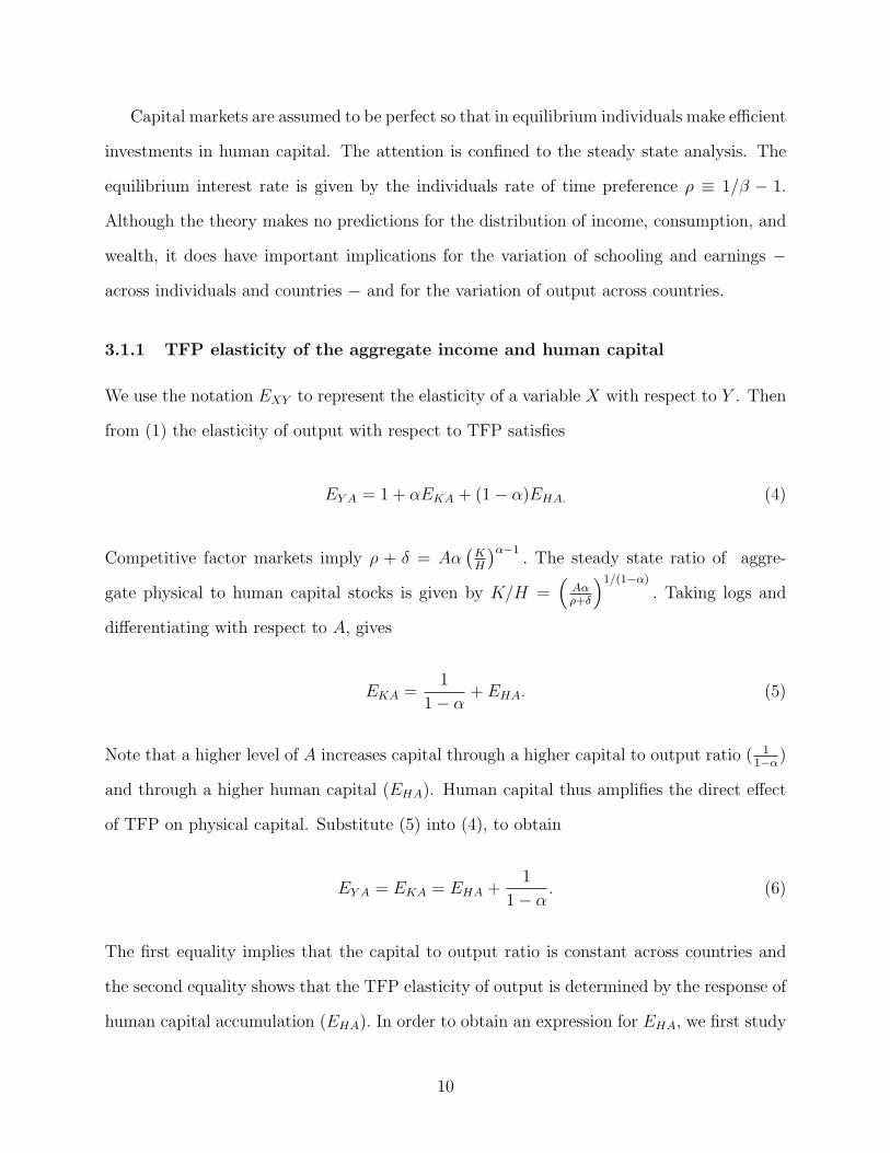
3.1.1 TFP elasticity of the aggregate income and human capital

We use the notation EXY to represent the elasticity of a variable X with respect to Y . Then

from (1) the elasticity of output with respect to TFP satisfies

EY A = 1 + αEKA + (1− α)EHA. (4)

Competitive factor markets imply ρ + δ = Aα(

KH

)α−1. The steady state ratio of aggre-

gate physical to human capital stocks is given by K/H =(

Aαρ+δ

)1/(1−α)

. Taking logs and

differentiating with respect to A, gives

EKA =1

1− α+ EHA. (5)

Note that a higher level of A increases capital through a higher capital to output ratio ( 11−α

)

and through a higher human capital (EHA). Human capital thus amplifies the direct effect

of TFP on physical capital. Substitute (5) into (4), to obtain

EY A = EKA = EHA +1

1− α. (6)

The first equality implies that the capital to output ratio is constant across countries and

the second equality shows that the TFP elasticity of output is determined by the response of

human capital accumulation (EHA). In order to obtain an expression for EHA, we first study

10

the decisions of individuals regarding human capital investments and we then aggregate the

behavior of individuals to obtain an aggregate elasticity.

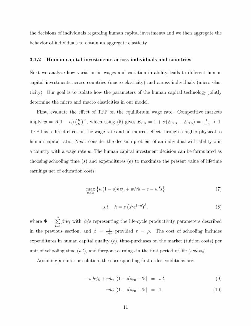
3.1.2 Human capital investments across individuals and countries

Next we analyze how variation in wages and variation in ability leads to different human

capital investments across countries (macro elasticity) and across individuals (micro elas-

ticity). Our goal is to isolate how the parameters of the human capital technology jointly

determine the micro and macro elasticities in our model.

First, evaluate the effect of TFP on the equilibrium wage rate. Competitive markets

imply w = A(1 − α)(

KH

)α, which using (5) gives EwA = 1 + α(EKA − EHA) = 1

1−α> 1.

TFP has a direct effect on the wage rate and an indirect effect through a higher physical to

human capital ratio. Next, consider the decision problem of an individual with ability z in

a country with a wage rate w. The human capital investment decision can be formulated as

choosing schooling time (s) and expenditures (e) to maximize the present value of lifetime

earnings net of education costs:

maxe,s,h

{w(1− s)hψ0 + whΨ− e− wls

}(7)

s.t. h = z(sηe1−η

)ξ, (8)

where Ψ =3∑

i=1

βiψi with ψi’s representing the life-cycle productivity parameters described

in the previous section, and β = 11+r

provided r = ρ. The cost of schooling includes

expenditures in human capital quality (e), time-purchases on the market (tuition costs) per

unit of schooling time (wl), and foregone earnings in the first period of life (swhψ0).

Assuming an interior solution, the corresponding first order conditions are:

−whψ0 + whs [(1− s)ψ0 + Ψ] = wl, (9)

whe [(1− s)ψ0 + Ψ] = 1, (10)

11

where hs = hsηξ and he = h

e(1− η) ξ. These equations can be expressed as

z(sηe1−η

)ξ{−ψ0 +

ηξ

s[(1− s)ψ0 + Ψ]

}= l (11)

e ={wz (1− η) ξ [(1− s)ψ0 + Ψ] sηξ

} 11−(1−η)ξ (12)

We are ready to analyze how individual decisions depend on the parameters of the maxi-

mization problem. In the absence of tuition costs (l = 0), it is easy to solve for s from (11)

and verify that the optimal quantity of schooling does not vary across individuals (z) and

countries (w). We thus maintain l > 0. Similarly, if the absence of education expenditures

(η = 1), the quality of schooling does not vary across individuals and countries. On the

contrary, when 0 < η < 1, equations (11) and (12) imply that both quantity and quality of

schooling vary across individuals (z) and countries (w).

Proposition 1: The theory requires l > 0 and 0 < η < 1 in order to generate differences

in the quantity and quality of schooling across individuals (z) and countries (A).

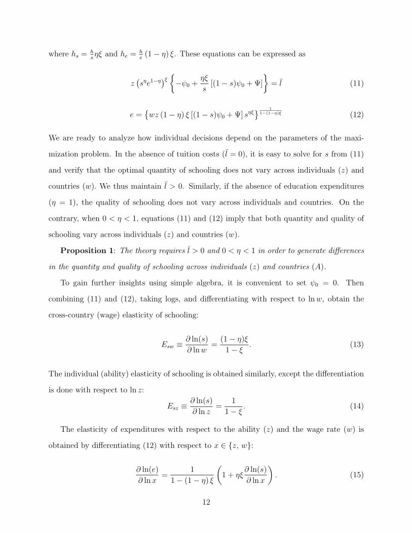
To gain further insights using simple algebra, it is convenient to set ψ0 = 0. Then

combining (11) and (12), taking logs, and differentiating with respect to lnw, obtain the

cross-country (wage) elasticity of schooling:

Esw ≡∂ ln(s)

∂ lnw=

(1− η)ξ

1− ξ. (13)

The individual (ability) elasticity of schooling is obtained similarly, except the differentiation

is done with respect to ln z:

Esz ≡∂ ln(s)

∂ ln z=

1

1− ξ. (14)

The elasticity of expenditures with respect to the ability (z) and the wage rate (w) is

obtained by differentiating (12) with respect to x ∈ {z, w}:

∂ ln(e)

∂ lnx=

1

1− (1− η) ξ

(1 + ηξ

∂ ln(s)

∂ lnx

). (15)

12

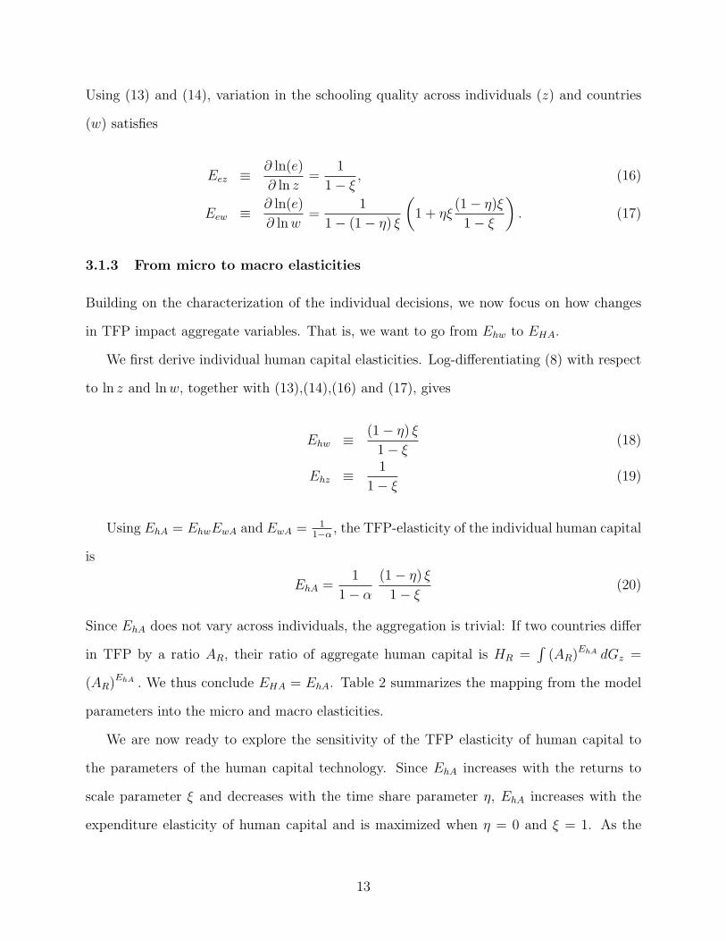
Using (13) and (14), variation in the schooling quality across individuals (z) and countries

(w) satisfies

Eez ≡ ∂ ln(e)

∂ ln z=

1

1− ξ, (16)

Eew ≡ ∂ ln(e)

∂ lnw=

1

1− (1− η) ξ

(1 + ηξ

(1− η)ξ

1− ξ

). (17)

3.1.3 From micro to macro elasticities

Building on the characterization of the individual decisions, we now focus on how changes

in TFP impact aggregate variables. That is, we want to go from Ehw to EHA.

We first derive individual human capital elasticities. Log-differentiating (8) with respect

to ln z and lnw, together with (13),(14),(16) and (17), gives

Ehw ≡ (1− η) ξ

1− ξ(18)

Ehz ≡ 1

1− ξ(19)

Using EhA = EhwEwA and EwA = 11−α

, the TFP-elasticity of the individual human capital

is

EhA =1

1− α

(1− η) ξ

1− ξ(20)

Since EhA does not vary across individuals, the aggregation is trivial: If two countries differ

in TFP by a ratio AR, their ratio of aggregate human capital is HR =∫

(AR)EhA dGz =

(AR)EhA . We thus conclude EHA = EhA. Table 2 summarizes the mapping from the model

parameters into the micro and macro elasticities.

We are now ready to explore the sensitivity of the TFP elasticity of human capital to

the parameters of the human capital technology. Since EhA increases with the returns to

scale parameter ξ and decreases with the time share parameter η, EhA increases with the

expenditure elasticity of human capital and is maximized when η = 0 and ξ = 1. As the

13

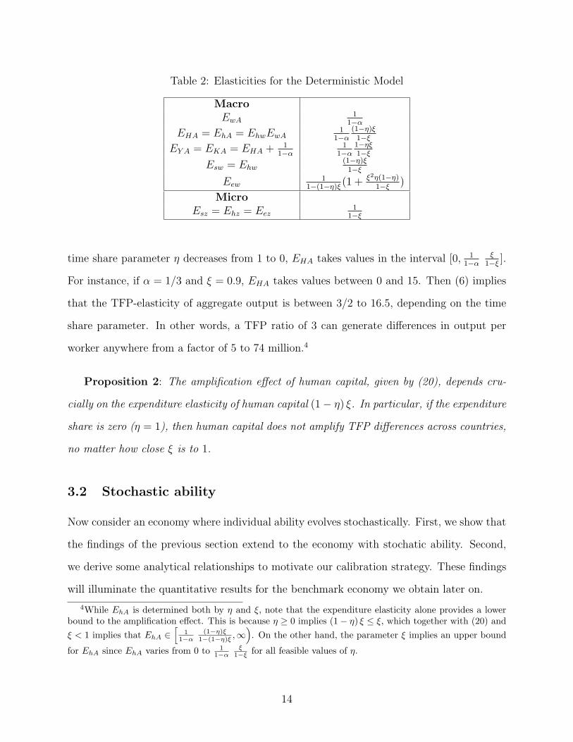
Table 2: Elasticities for the Deterministic Model

MacroEwA

11−α

EHA = EhA = EhwEwA1

1−α(1−η)ξ1−ξ

EY A = EKA = EHA + 11−α

11−α

1−ηξ1−ξ

Esw = Ehw(1−η)ξ1−ξ

Eew1

1−(1−η)ξ(1 + ξ2η(1−η)

1−ξ)

MicroEsz = Ehz = Eez

11−ξ

time share parameter η decreases from 1 to 0, EHA takes values in the interval [0, 11−α

ξ1−ξ

].

For instance, if α = 1/3 and ξ = 0.9, EHA takes values between 0 and 15. Then (6) implies

that the TFP-elasticity of aggregate output is between 3/2 to 16.5, depending on the time

share parameter. In other words, a TFP ratio of 3 can generate differences in output per

worker anywhere from a factor of 5 to 74 million.4

Proposition 2: The amplification effect of human capital, given by (20), depends cru-

cially on the expenditure elasticity of human capital (1− η) ξ. In particular, if the expenditure

share is zero (η = 1), then human capital does not amplify TFP differences across countries,

no matter how close ξ is to 1.

3.2 Stochastic ability

Now consider an economy where individual ability evolves stochastically. First, we show that

the findings of the previous section extend to the economy with stochatic ability. Second,

we derive some analytical relationships to motivate our calibration strategy. These findings

will illuminate the quantitative results for the benchmark economy we obtain later on.

4While EhA is determined both by η and ξ, note that the expenditure elasticity alone provides a lowerbound to the amplification effect. This is because η ≥ 0 implies (1− η) ξ ≤ ξ, which together with (20) andξ < 1 implies that EhA ∈

[1

1−α(1−η)ξ

1−(1−η)ξ ,∞). On the other hand, the parameter ξ implies an upper bound

for EhA since EhA varies from 0 to 11−α

ξ1−ξ for all feasible values of η.

14

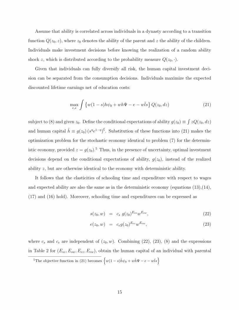
Assume that ability is correlated across individuals in a dynasty according to a transition

function Q(z0, z), where z0 denotes the ability of the parent and z the ability of the children.

Individuals make investment decisions before knowing the realization of a random ability

shock z, which is distributed according to the probability measure Q(z0, ·).

Given that individuals can fully diversify all risk, the human capital investment deci-

sion can be separated from the consumption decisions. Individuals maximize the expected

discounted lifetime earnings net of education costs:

maxe,s

∫ {w(1− s)hψ0 + whΨ− e− wls

}Q(z0, dz) (21)

subject to (8) and given z0. Define the conditional expectations of ability g(z0) ≡∫zQ(z0, dz)

and human capital h ≡ g(z0) (sηe1−η)ξ. Substitution of these functions into (21) makes the

optimization problem for the stochastic economy identical to problem (7) for the determin-

istic economy, provided z = g(z0).5 Thus, in the presence of uncertainty, optimal investment

decisions depend on the conditional expectations of ability, g(z0), instead of the realized

ability z, but are otherwise identical to the economy with deterministic ability.

It follows that the elasticities of schooling time and expenditure with respect to wages

and expected ability are also the same as in the deterministic economy (equations (13),(14),

(17) and (16) hold). Moreover, schooling time and expenditures can be expressed as

s(z0, w) = cs g(z0)EszwEsw , (22)

e(z0, w) = ceg(z0)EezwEew , (23)

where cs and ce are independent of (z0, w). Combining (22), (23), (8) and the expressions

in Table 2 for (Esz, Esw, Eez, Eew), obtain the human capital of an individual with parental

5The objective function in (21) becomes{w(1− s)hψ0 + whΨ− e− wls

}

15

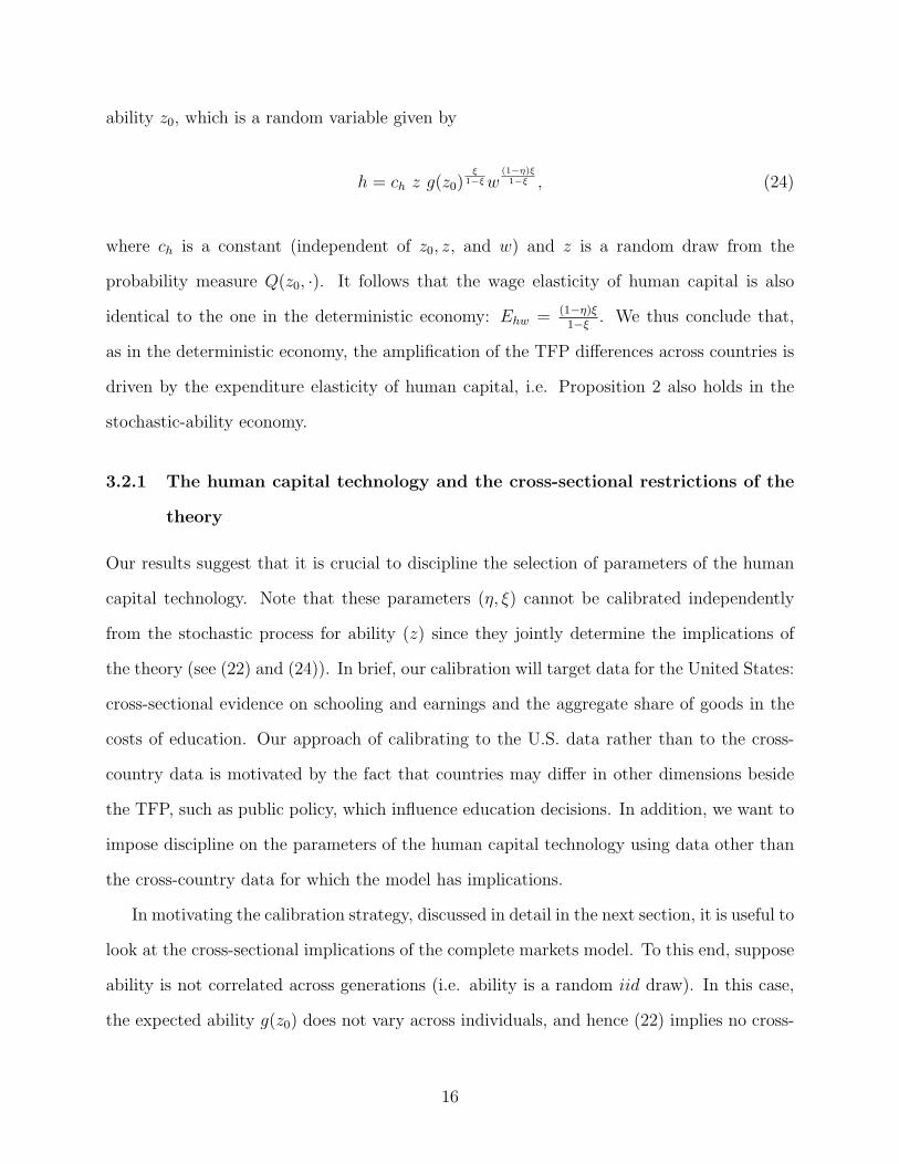
ability z0, which is a random variable given by

h = ch z g(z0)ξ

1−ξw(1−η)ξ1−ξ , (24)

where ch is a constant (independent of z0, z, and w) and z is a random draw from the

probability measure Q(z0, ·). It follows that the wage elasticity of human capital is also

identical to the one in the deterministic economy: Ehw = (1−η)ξ1−ξ

. We thus conclude that,

as in the deterministic economy, the amplification of the TFP differences across countries is

driven by the expenditure elasticity of human capital, i.e. Proposition 2 also holds in the

stochastic-ability economy.

3.2.1 The human capital technology and the cross-sectional restrictions of the

theory

Our results suggest that it is crucial to discipline the selection of parameters of the human

capital technology. Note that these parameters (η, ξ) cannot be calibrated independently

from the stochastic process for ability (z) since they jointly determine the implications of

the theory (see (22) and (24)). In brief, our calibration will target data for the United States:

cross-sectional evidence on schooling and earnings and the aggregate share of goods in the

costs of education. Our approach of calibrating to the U.S. data rather than to the cross-

country data is motivated by the fact that countries may differ in other dimensions beside

the TFP, such as public policy, which influence education decisions. In addition, we want to

impose discipline on the parameters of the human capital technology using data other than

the cross-country data for which the model has implications.

In motivating the calibration strategy, discussed in detail in the next section, it is useful to

look at the cross-sectional implications of the complete markets model. To this end, suppose

ability is not correlated across generations (i.e. ability is a random iid draw). In this case,

the expected ability g(z0) does not vary across individuals, and hence (22) implies no cross-

16

sectional variation in schooling. Thus, ability shocks need to be serially correlated for the

theory to be consistent with the cross-sectional evidence on schooling. Moreover, if ability

shocks were perfectly correlated across generations, then z = g(z0) = z0 and (24) implies

that there is no variation in earnings across individuals with the same level of schooling. To

sum up, ability shocks need to be imperfectly correlated across generations for the theory to

be consistent with the cross-sectional evidence on schooling and earnings.

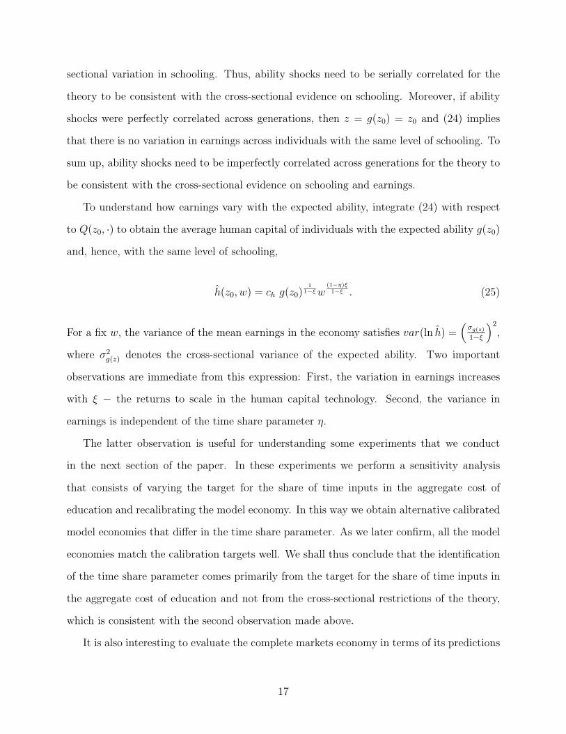
To understand how earnings vary with the expected ability, integrate (24) with respect

to Q(z0, ·) to obtain the average human capital of individuals with the expected ability g(z0)

and, hence, with the same level of schooling,

h(z0, w) = ch g(z0)1

1−ξw(1−η)ξ1−ξ . (25)

For a fix w, the variance of the mean earnings in the economy satisfies var(ln h) =(

σg(z)

1−ξ

)2

,

where σ2g(z) denotes the cross-sectional variance of the expected ability. Two important

observations are immediate from this expression: First, the variation in earnings increases

with ξ − the returns to scale in the human capital technology. Second, the variance in

earnings is independent of the time share parameter η.

The latter observation is useful for understanding some experiments that we conduct

in the next section of the paper. In these experiments we perform a sensitivity analysis

that consists of varying the target for the share of time inputs in the aggregate cost of

education and recalibrating the model economy. In this way we obtain alternative calibrated

model economies that differ in the time share parameter. As we later confirm, all the model

economies match the calibration targets well. We shall thus conclude that the identification

of the time share parameter comes primarily from the target for the share of time inputs in

the aggregate cost of education and not from the cross-sectional restrictions of the theory,

which is consistent with the second observation made above.

It is also interesting to evaluate the complete markets economy in terms of its predictions

17

for the quality of immigrants by country of origin. Consider an economy that has a large

number of immigrants born in two countries that differ in their TFP. We assume that,

conditional on a schooling level, immigration is a random draw from the population in each

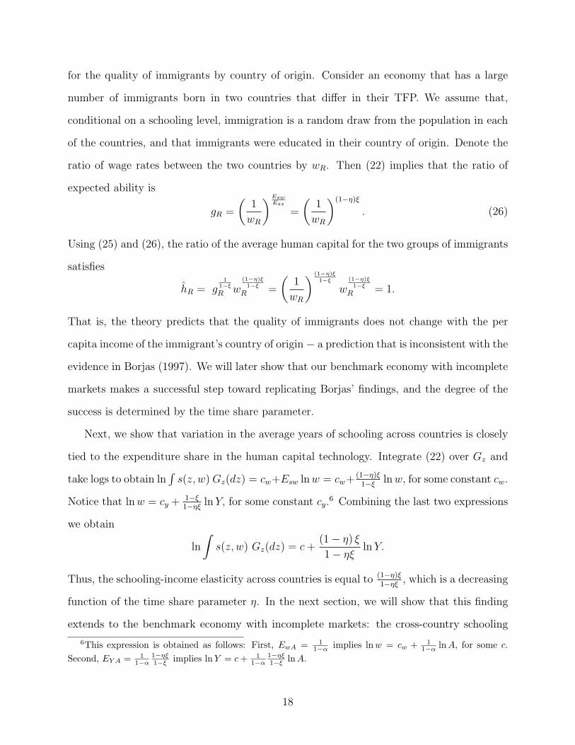
of the countries, and that immigrants were educated in their country of origin. Denote the

ratio of wage rates between the two countries by wR. Then (22) implies that the ratio of

expected ability is

gR =

(1

wR

)EswEsz

=

(1

wR

)(1−η)ξ

. (26)

Using (25) and (26), the ratio of the average human capital for the two groups of immigrants

satisfies

hR = g1

1−ξ

R w(1−η)ξ1−ξ

R =

(1

wR

) (1−η)ξ1−ξ

w(1−η)ξ1−ξ

R = 1.

That is, the theory predicts that the quality of immigrants does not change with the per

capita income of the immigrant’s country of origin− a prediction that is inconsistent with the

evidence in Borjas (1997). We will later show that our benchmark economy with incomplete

markets makes a successful step toward replicating Borjas’ findings, and the degree of the

success is determined by the time share parameter.

Next, we show that variation in the average years of schooling across countries is closely

tied to the expenditure share in the human capital technology. Integrate (22) over Gz and

take logs to obtain ln∫s(z, w)Gz(dz) = cw+Esw lnw = cw+ (1−η)ξ

1−ξlnw, for some constant cw.

Notice that lnw = cy + 1−ξ1−ηξ

lnY, for some constant cy.6 Combining the last two expressions

we obtain

ln

∫s(z, w) Gz(dz) = c+

(1− η) ξ

1− ηξlnY.

Thus, the schooling-income elasticity across countries is equal to (1−η)ξ1−ηξ

, which is a decreasing

function of the time share parameter η. In the next section, we will show that this finding

extends to the benchmark economy with incomplete markets: the cross-country schooling

6This expression is obtained as follows: First, EwA = 11−α implies lnw = cw + 1

1−α lnA, for some c.Second, EY A = 1

1−α1−ηξ1−ξ implies lnY = c+ 1

1−α1−ηξ1−ξ lnA.

18

elasticity with respect to income declines with η.

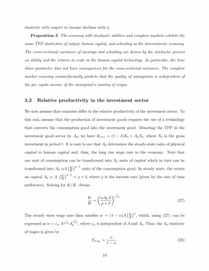
Proposition 3: The economy with stochastic abilities and complete markets exhibits the

same TFP elasticities of output, human capital, and schooling as the deterministic economy.

The cross-sectional variances of earnings and schooling are driven by the stochastic process

on ability and the returns to scale in the human capital technology. In particular, the time

share parameter does not have consequences for the cross-sectional variances. The complete

market economy counterfactually predicts that the quality of immigrants is independent of

the per capita income of the immigrant’s country of origin.

3.3 Relative productivity in the investment sector

We now assume that countries differ in the relative productivity of the investment sector. To

this end, assume that the production of investment goods requires the use of a technology

that converts the consumption good into the investment good. Denoting the TFP in the

investment good sector by Ak, we have Kt+1 = (1 − δ)Kt + AkXt, where Xt is the gross

investment in period t. It is easy to see that Ak determines the steady-state ratio of physical

capital to human capital and, thus, the long run wage rate in the economy. Note that

one unit of consumption can be transformed into Ak units of capital which in turn can be

transformed into Ak αA(

KH

)α−1units of the consumption good. In steady state, the return

on capital Ak α A(

KH

)α−1= ρ + δ, where ρ is the interest rate (given by the rate of time

preference). Solving for K/H, obtain

K

H=

(αAkA

ρ+ δ

) 11−α

. (27)

The steady state wage rate then satisfies w = (1 − α)A(

KH

)α, which, using (27), can be

expressed as w = cw A1

1−αAα

1−α

k , where cw is independent of A and Ak. Thus, the Ak elasticity

of wages is given by

EwAk=

α

1− α. (28)

19

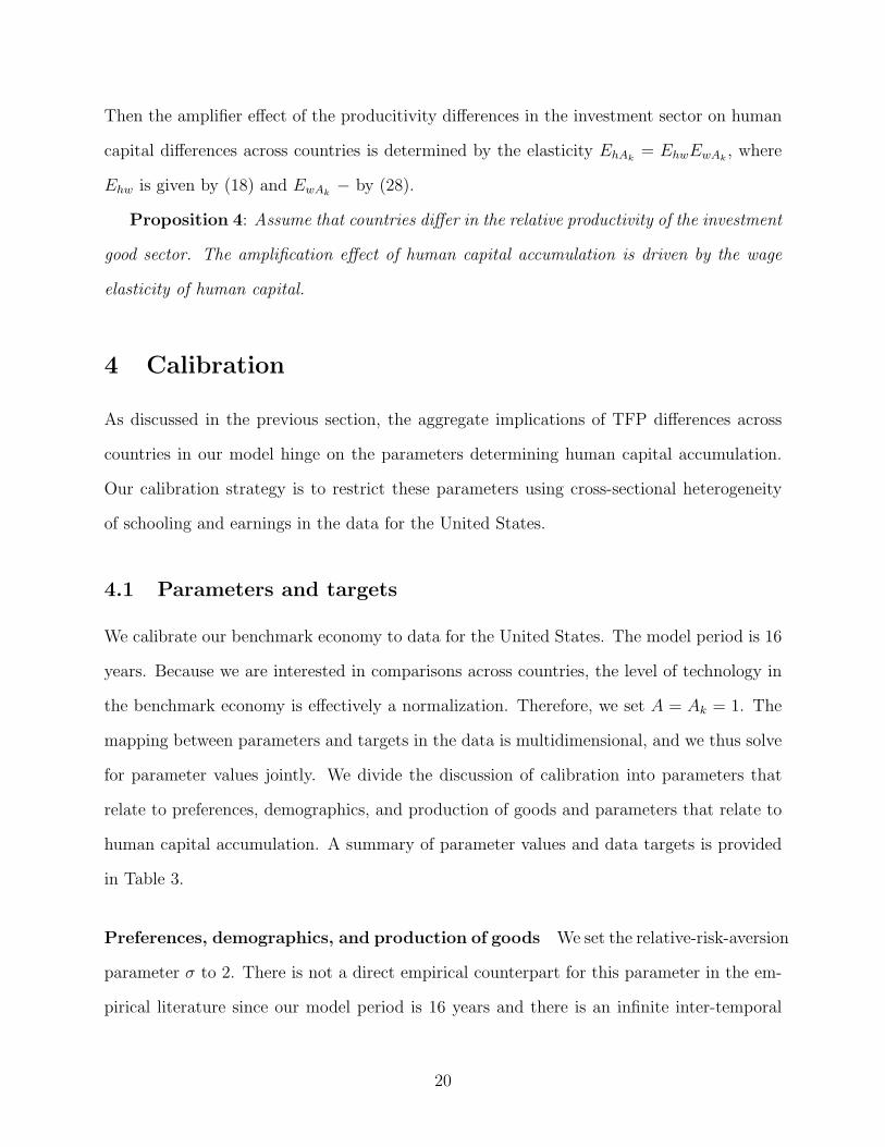
Then the amplifier effect of the producitivity differences in the investment sector on human

capital differences across countries is determined by the elasticity EhAk= EhwEwAk

, where

Ehw is given by (18) and EwAk− by (28).

Proposition 4: Assume that countries differ in the relative productivity of the investment

good sector. The amplification effect of human capital accumulation is driven by the wage

elasticity of human capital.

4 Calibration

As discussed in the previous section, the aggregate implications of TFP differences across

countries in our model hinge on the parameters determining human capital accumulation.

Our calibration strategy is to restrict these parameters using cross-sectional heterogeneity

of schooling and earnings in the data for the United States.

4.1 Parameters and targets

We calibrate our benchmark economy to data for the United States. The model period is 16

years. Because we are interested in comparisons across countries, the level of technology in

the benchmark economy is effectively a normalization. Therefore, we set A = Ak = 1. The

mapping between parameters and targets in the data is multidimensional, and we thus solve

for parameter values jointly. We divide the discussion of calibration into parameters that

relate to preferences, demographics, and production of goods and parameters that relate to

human capital accumulation. A summary of parameter values and data targets is provided

in Table 3.

Preferences, demographics, and production of goods We set the relative-risk-aversion

parameter σ to 2. There is not a direct empirical counterpart for this parameter in the em-

pirical literature since our model period is 16 years and there is an infinite inter-temporal

20

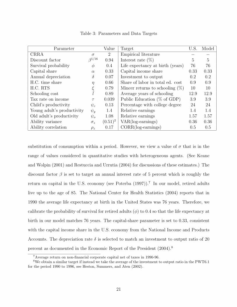
Table 3: Parameters and Data Targets

Parameter Value Target U.S. ModelCRRA σ 2 Empirical literature − −Discount factor β1/16 0.94 Interest rate (%) 5 5Survival probability φ 0.4 Life expectancy at birth (years) 76 76Capital share α 0.33 Capital income share 0.33 0.33Annual depreciation δ 0.07 Investment to output 0.2 0.2H.C. time share η 0.66 Share of labor in total ed. cost 0.9 0.9H.C. RTS ξ 0.79 Mincer returns to schooling (%) 10 10Schooling cost l 0.89 Average years of schooling 12.9 12.9Tax rate on income τ 0.039 Public Education (% of GDP) 3.9 3.9Child’s productivity ψc 0.13 Percentage with college degree 24 24Young adult’s productivity ψy 1.4 Relative earnings 1.4 1.4Old adult’s productivity ψo 1.08 Relative earnings 1.57 1.57Ability variance σz (0.51)2 VAR(log-earnings) 0.36 0.36Ability correlation ρz 0.17 CORR(log-earnings) 0.5 0.5

substitution of consumption within a period. However, we view a value of σ that is in the

range of values considered in quantitative studies with heterogeneous agents. (See Keane

and Wolpin (2001) and Restuccia and Urrutia (2004) for discussions of these estimates.) The

discount factor β is set to target an annual interest rate of 5 percent which is roughly the

return on capital in the U.S. economy (see Poterba (1997)).7 In our model, retired adults

live up to the age of 85. The National Center for Health Statistics (2004) reports that in

1990 the average life expectancy at birth in the United States was 76 years. Therefore, we

calibrate the probability of survival for retired adults (φ) to 0.4 so that the life expectancy at

birth in our model matches 76 years. The capital-share parameter is set to 0.33, consistent

with the capital income share in the U.S. economy from the National Income and Products

Accounts. The depreciation rate δ is selected to match an investment to output ratio of 20

percent as documented in the Economic Report of the President (2004).8

7Average return on non-financial corporate capital net of taxes in 1990-96.8We obtain a similar target if instead we take the average of the investment to output ratio in the PWT6.1

for the period 1990 to 1996, see Heston, Summers, and Aten (2002).

21

Human capital accumulation Recall that the human capital technology is given by

h′ = z′ (sηe1−η)ξ, where s denotes schooling time and e denotes educational expenditures.

We need to specify two elasticity parameters: η and ξ. Ability follows an AR(1) process (in

logs):

log(z′) = ρz log(z) + εz,

where εz ∼ N(0, σz). In our computations, we approximate this stochastic process with a

discrete first-order Markov chain that takes 7 possible values for ability z. We use the approx-

imation procedure in Tauchen (1986) to compute transition probabilities. This procedure

involves selecting two additional parameter values: ρz and σz. There are five additional

parameters affecting human capital accumulation: Schooling cost l, tax rate on income τ

(that in equilibrium determines public education subsidies p), and life-cycle productivity

parameters (ψc, ψy, ψo), setting the relative labor earnings of children, young adults, and

old adults. Our calibration procedure restricts the values of these 9 parameters so that the

equilibrium of the model matches the following 9 targets from the U.S. data:

1. Intergenerational correlation of log-earnings of 0.5 from Mulligan (1997). (See also

excellent surveys of the empirical literature on the intergenerational correlation of

earnings by Stokey (1998) and Solon (1999))

2. Variance of log permanent earnings of 0.36 (see Mulligan (1997, 1999))

3. Average years of schooling of 12.9 from the U.S. Department of Education (2004) in

1990. (See also Barro and Lee (1996).)

4. Fraction of individuals with a college degree or more of 24 percent from the Historical

Tables of the U.S. Census Bureau (2004).

5. Public education expenditures as a fraction of GDP of 3.9 percent from the Statistical

Abstract of the United States (1999). In computing this statistic in the data, we

treat as public expenditures all state and federal expenditures. We exclude public

22

local expenditures in education because these expenditures are closely tied to property

values and therefore to the income of parents. (See Restuccia and Urrutia (2004) for

a discussion.)

6. The ratio of earnings for full-time, year-round workers of ages 35-54 to ages 25-34 of

1.40 in 2003 from the U.S. Census Bureau, Historical Income Tables.

7. The ratio of earnings for full-time, year-round workers of ages 55-64 to ages 25-34 of

1.57 in 2003 from the U.S. Census Bureau, Historical Income Tables.

8. Mincer returns to schooling of 10 percent. Heckman et al. (2005) report a Mincer

return of between 10 to 13 percent during the period 1980 to 1990. Psacharopoulos

(1994) estimates a Mincer return of 10 percent for the United States for the period

1990-95. Because Psacharopoulos also provides data on Mincer returns for a large set

of countries, we follow Bils and Klenow (2000) in using Psacharopoulos’ estimate for

the U.S. economy. In the benchmark economy, we measure returns to education by

regressing log-wages on years of education:

log(wh′i) = b0 + b1 (16si) + ui,

where b1 gives the Mincer return.

9. The share of labor inputs in the total cost of investment in education of 90 percent

according to Kendrick (1976) and the U.S. Department of Education (1996).

4.2 The benchmark economy

The benchmark economy matches all the calibration targets well (see Table 3). In particular,

it successfully replicates the U.S. cross-sectional data on schooling (Mincer return, average

years of schooling, fraction of college-educated individuals), earnings (variance and intergen-

erational correlation of earnings), and the share of labor inputs in total education costs. We

23

now show that the model is consistent with several dimensions of heterogeneity in the data

that were not targeted in the calibration. We conclude that the model is a good quantitative

theory of within-country heterogeneity.

Distribution of Schooling According to the U.S. Department of Education (2004) the

proportion of people in 1990 between 25 and 34 years of age (all sexes and races) with

primary schooling (1st to 8th grade) as their highest education attainment was 4 percent,

with secondary schooling (9th to 12th grade) − 50 percent, and with college education (4

years of college or more) − 24 percent. Our model matches these statistics reasonably well

as documented in Table 4.9

Table 4: Education and Earnings − Model and Data

Schooling Dist. Rel. Earnings Mincer Ret.(%)Model Data Model Data Model Data

Primary 0.08 0.04 0.66 0.62 15.6 21.8Secondary 0.28 0.50 1.00 1.00 9.3 11.5College 0.24 0.24 1.78 1.70 10.3 9.6

Mincer returns data from Willis (1986).

Schooling and earnings The benchmark economy matches the joint distribution of earn-

ings and schooling in the data well. According to the U.S. Department of Education (2004),

in 1998 males in the U.S. with college education earn (on average) 70 percent more than

high-school graduates. This earning ratio is 1.78 in the benchmark economy. Similarly, the

earnings ratio between individual with primary education and secondary education is .62 in

the U.S. data and it is .66 in the model economy (see Table 4). Recall that the the calibration

targeted the average Mincer returns to education. Nonetheless, the benchmark economy is

also consistent with the fact that in the data Mincer returns are substantially higher at low

9We note, however, that time in school is a continuous variable in our model, making its comparisonwith the data non trivial. In particular, the distribution of schooling in the data has clear spikes at levels ofeducation where an educational degree is completed.

24

levels of schooling. In the benchmark economy and in the U.S. data, earnings vary not only

across individuals with different years of schooling but also across individuals with the same

level of schooling. To evaluate the importance of earnings inequality within schooling groups

in the benchmark economy, we simulate individual level data on schooling and earnings. We

then regress log earnings on schooling years and obtain an R2 of only 26.5 percent. Thus, the

regression results imply that schooling accounts for a low fraction of the variance in earnings

across individuals which is consistent with the findings in the labor literature for the United

States (see for instance Neal and Johnson (1996)).

Expenditures on education The share of GDP spent on education increases with the

returns to scale parameter in the human capital production function as discussed in our

calibration section. In light of that discussion, it is interesting to compare the proportion

of GDP in the form of educational expenditures in our model with the data. Haveman and

Wolfe (1995) report that expenditures on children aged 0-18 are as large as 14.5 percent of

GDP. This share includes not only public investment, but also private costs, such as food,

housing, transportation and foregone parental earnings in child care. When we exclude

foregone parental earnings from Haveman and Wolfe’s numbers we obtain 12.6 percent. In

our model, total education expenditures correspond to (e+wls) aggregated over all people.

In the benchmark economy and using this formula, total expenditures on education amount

to 12 percent of GDP, a figure close to Haveman and Wolfe’s estimate.

5 Quantitative results

We use our quantitative theory to assess the aggregate and distributional consequences of

TFP differences across countries. Changes in TFP affect human capital accumulation since

human capital investment requires goods in our calibrated model economy (see the discussion

in Section 3). The question we address in this section is about the quantitative magnitude of

this effect. We find that TFP has a large effect on human capital accumulation and output

25

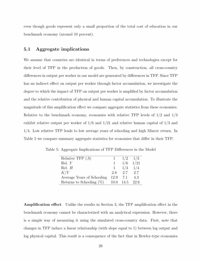
even though goods represent only a small proportion of the total cost of education in our

benchmark economy (around 10 percent).

5.1 Aggregate implications

We assume that countries are identical in terms of preferences and technologies except for

their level of TFP in the production of goods. Then, by construction, all cross-country

differences in output per worker in our model are generated by differences in TFP. Since TFP

has an indirect effect on output per worker through factor accumulation, we investigate the

degree to which the impact of TFP on output per worker is amplified by factor accumulation

and the relative contribution of physical and human capital accumulation. To illustrate the

magnitude of this amplification effect we compare aggregate statistics from these economies.

Relative to the benchmark economy, economies with relative TFP levels of 1/2 and 1/3

exhibit relative output per worker of 1/6 and 1/21 and relative human capital of 1/3 and

1/4. Low relative TFP leads to low average years of schooling and high Mincer return. In

Table 5 we compare summary aggregate statistics for economies that differ in their TFP.

Table 5: Aggregate Implications of TFP Differences in the Model

Relative TFP (A) 1 1/2 1/3Rel. Y 1 1/6 1/21Rel. H 1 1/3 1/4K/Y 2.8 2.7 2.7Average Years of Schooling 12.9 7.1 4.3Returns to Schooling (%) 10.0 14.5 22.6

Amplification effect Unlike the results in Section 3, the TFP amplification effect in the

benchmark economy cannot be characterized with an analytical expression. However, there

is a simple way of measuring it using the simulated cross-country data. First, note that

changes in TFP induce a linear relationship (with slope equal to 1) between log output and

log physical capital. This result is a consequence of the fact that in Bewley-type economies

26

(dynastic economies with uninsurable idiosyncratic risk), the equilibrium interest rate is close

to the rate of time preference (see for instance Aiyagari (1994) and Fuster (2000)). As a

result, in equilibrium the marginal product of capital is close to the rate of time preference

plus the depreciation rate of capital, i.e., ∂y∂k

= α yk≈ ρ + δ. Using this relationship to solve

for k as a function of output we obtain k = cky for some constant ck. Second, as indicated in

Figure 1, the model implies a linear relationship between log human capital and log output

as TFP varies across economies, but the slope of this relationship is less than one. Using this

observation, we write human capital as a function of output as log(h) = ch + γ log(y), which

implies that h = exp(ch)yγ. Substituting the expressions derived for k and h (in terms of y)

in the production function of goods and solving for y we obtain

y = cyA1

(1−α)(1−γ) , (29)

for some constant cy. Then, the TFP elasticity of output per worker in our model is 1(1−α)(1−γ)

.

In the benchmark economy, α = 0.33 and γ = 0.46 (as indicated by the slope coefficient in

Figure 1). As a result, the TFP elasticity of output per worker is equal to 2.77. It follows

that if TFP differs by a factor of 2 between two economies, the model implies that their

output per worker would differ by a factor of 22.77 = 6.8. Another way of expressing this

result is to compute the TFP differences required in the model to generate a given difference

in output per worker between two countries. From equation (29), the ratio of output per

worker between any arbitrary economies i and j is related to their relative TFP levels:

yi

yj

=

(Ai

Aj

) 1(1−α)(1−γ)

.

Using an elasticity of 2.77 from our previous calculations, it follows that an output ratio of

20 can be generated by a TFP ratio of 2.94. We thus conclude that our calibrated model

implies a large amplification effect of TFP differences across countries. Moreover, we note

that the amplification effect provided by physical capital is 11−α

= 1.49 and the one provided

27

by human capital is 11−γ

= 1.85. Human capital thus represents an important source of

amplification.

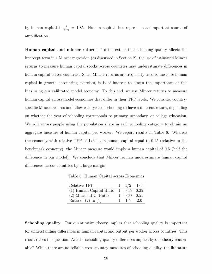
Human capital and mincer returns To the extent that schooling quality affects the

intercept term in a Mincer regression (as discussed in Section 2), the use of estimated Mincer

returns to measure human capital stocks across countries may underestimate differences in

human capital across countries. Since Mincer returns are frequently used to measure human

capital in growth accounting exercises, it is of interest to assess the importance of this

bias using our calibrated model economy. To this end, we use Mincer returns to measure

human capital across model economies that differ in their TFP levels. We consider country-

specific Mincer returns and allow each year of schooling to have a different return, depending

on whether the year of schooling corresponds to primary, secondary, or college education.

We add across people using the population share in each schooling category to obtain an

aggregate measure of human capital per worker. We report results in Table 6. Whereas

the economy with relative TFP of 1/3 has a human capital equal to 0.25 (relative to the

benchmark economy), the Mincer measure would imply a human capital of 0.5 (half the

difference in our model). We conclude that Mincer returns underestimate human capital

differences across countries by a large margin.

Table 6: Human Capital across Economies

Relative TFP 1 1/2 1/3(1) Human Capital Ratio 1 0.45 0.25(2) Mincer H.C. Ratio 1 0.69 0.51Ratio of (2) to (1) 1 1.5 2.0

Schooling quality Our quantitative theory implies that schooling quality is important

for understanding differences in human capital and output per worker across countries. This

result raises the question: Are the schooling-quality differences implied by our theory reason-

able? While there are no reliable cross-country measures of schooling quality, the literature

28

has used the empirical evidence on earnings of immigrants as an indirect approach to mea-

suring human capital differences across countries. Therefore, it is of interest to compare

our findings with those of Borjas (1987). Looking at immigrant wages in the United States,

Borjas estimates that, on average, the wage that a worker with a given amount of educa-

tion earns in the United States is 0.12 percent higher when the income per person in the

immigrant’s country of origin is 1 percent higher.

Table 7 shows that the average earnings of a person in the benchmark economy is between

3.5 and 4 times the average earnings of a similar worker in the economy with relative TFP

level of 1/2 (depending on the schooling level of the person) and it is more than 7 times

the earnings of an equally educated worker in a country with relative TFP level of 1/3.

The earnings ratio is largest for people with primary education. The bulk of cross-country

earnings differences can be attributed to differences in relative prices. If a person from the

economy with relative TFP of 1/2 were to migrate to the benchmark economy, the wage rate

of this person would increase by a factor of 2.8. If the immigrant comes from an economy

with relative TFP of 1/3, his wage rate would increase by a factor of 5.2. Our model

is thus consistent with the observed migration pressures from poor to rich countries. On

average, immigrants in the benchmark economy would not earn the same as natives with the

same school years because of the differences in the quality of schooling (as captured by the

expenditure on education goods). Native workers with primary and college education in the

benchmark economy earn between 20 to 40 percent more than potential immigrants with

same level of schooling and born in the economy with relative TFP of 1/2. The information

in Table 7 can be used to obtain an estimate of the income elasticity of schooling quality (by

schooling level) across countries as follows:

ηquality,y =log(H1

Hj)

log(Y1

Yj),

where H1 and Y1 stand for human capital and per capita income in the benchmark economy

29

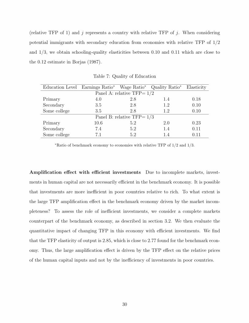
(relative TFP of 1) and j represents a country with relative TFP of j. When considering

potential immigrants with secondary education from economies with relative TFP of 1/2

and 1/3, we obtain schooling-quality elasticities between 0.10 and 0.11 which are close to

the 0.12 estimate in Borjas (1987).

Table 7: Quality of Education

Education Level Earnings Ratio∗ Wage Ratio∗ Quality Ratio∗ ElasticityPanel A: relative TFP= 1/2

Primary 4.0 2.8 1.4 0.18Secondary 3.5 2.8 1.2 0.10Some college 3.5 2.8 1.2 0.10

Panel B: relative TFP= 1/3Primary 10.6 5.2 2.0 0.23Secondary 7.4 5.2 1.4 0.11Some college 7.1 5.2 1.4 0.11

∗Ratio of benchmark economy to economies with relative TFP of 1/2 and 1/3.

Amplification effect with efficient investments Due to incomplete markets, invest-

ments in human capital are not necessarily efficient in the benchmark economy. It is possible

that investments are more inefficient in poor countries relative to rich. To what extent is

the large TFP amplification effect in the benchmark economy driven by the market incom-

pleteness? To assess the role of inefficient investments, we consider a complete markets

counterpart of the benchmark economy, as described in section 3.2. We then evaluate the

quantitative impact of changing TFP in this economy with efficient investments. We find

that the TFP elasticity of output is 2.85, which is close to 2.77 found for the benchmark econ-

omy. Thus, the large amplification effect is driven by the TFP effect on the relative prices

of the human capital inputs and not by the inefficiency of investments in poor countries.

30

5.2 Sensitivity analysis

Our baseline calibration targeted an expenditure share of time inputs of 90 percent as re-

ported by Kendrick (1976). We acknowledge that, despite Kendrick’s careful analysis, it may

be difficult to accurately measure inputs into human capital accumulation. Since the magni-

tude of our quantitative results hinge on the importance of time inputs, a sensitivity analysis

along this dimension is warranted.10 To this end, we consider three alternative calibrations

to our benchmark economy. In all the calibrated economies, we maintain the calibration

targets of our benchmark economy except for the share of time inputs in education costs,

which we set at 85, 95, and 100 percent (instead of 90 percent in the baseline calibration).

Our goal is to evaluate the effects of TFP under different assumptions about the importance

of time inputs in human capital accumulation. We then use data to discriminate among the

alternative specifications.

The three calibrated model economies do as well as the benchmark economy in matching

the targets discussed in section 4 (see Table 3).11 In other words, all the economies match the

data targets well, including the distributional statistics. Therefore, the economies considered

are equally good quantitative theories of the U.S. income distribution (as we have anticipated

in Section 3). However, there are a number of dimensions where these economies perform

differently. We discuss these differences in detail.

To start, we compute the TFP elasticity of output per worker in each of the calibrated

model economies and report the results in Table 8. When human capital requires only time

inputs, physical capital is the only source of amplification, and it implies a TFP elasticity of

1.49. When the share of time inputs is 95 percent, the TFP elasticity of income is 1.84. This

statistic increases to 2.8 in our baseline calibration and to 3.63 when time inputs represent

85 percent. Given these elasticity estimates, the amplification effect of TFP differences

10There is a related discussion in the taxation literature where the tax effect on human capital accumulationhinges on the importance of goods in the production of human capital. For instance, see Trostel (1993) andDavies and Whalley (1989).

11The parameter values needed to match the targets are available from the authors upon request.

31

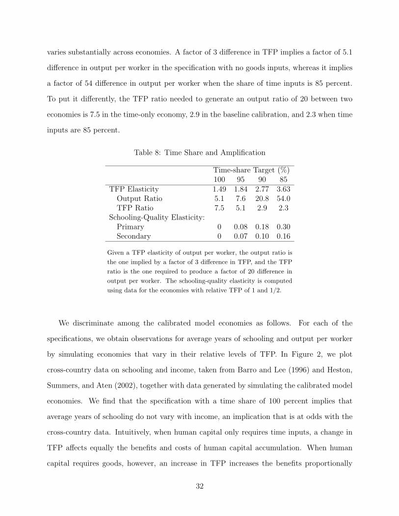
varies substantially across economies. A factor of 3 difference in TFP implies a factor of 5.1

difference in output per worker in the specification with no goods inputs, whereas it implies

a factor of 54 difference in output per worker when the share of time inputs is 85 percent.

To put it differently, the TFP ratio needed to generate an output ratio of 20 between two

economies is 7.5 in the time-only economy, 2.9 in the baseline calibration, and 2.3 when time

inputs are 85 percent.

Table 8: Time Share and Amplification

Time-share Target (%)100 95 90 85

TFP Elasticity 1.49 1.84 2.77 3.63Output Ratio 5.1 7.6 20.8 54.0TFP Ratio 7.5 5.1 2.9 2.3

Schooling-Quality Elasticity:Primary 0 0.08 0.18 0.30Secondary 0 0.07 0.10 0.16

Given a TFP elasticity of output per worker, the output ratio isthe one implied by a factor of 3 difference in TFP, and the TFPratio is the one required to produce a factor of 20 difference inoutput per worker. The schooling-quality elasticity is computedusing data for the economies with relative TFP of 1 and 1/2.

We discriminate among the calibrated model economies as follows. For each of the

specifications, we obtain observations for average years of schooling and output per worker

by simulating economies that vary in their relative levels of TFP. In Figure 2, we plot

cross-country data on schooling and income, taken from Barro and Lee (1996) and Heston,

Summers, and Aten (2002), together with data generated by simulating the calibrated model

economies. We find that the specification with a time share of 100 percent implies that

average years of schooling do not vary with income, an implication that is at odds with the

cross-country data. Intuitively, when human capital only requires time inputs, a change in

TFP affects equally the benefits and costs of human capital accumulation. When human

capital requires goods, however, an increase in TFP increases the benefits proportionally

32

more than the costs of human capital accumulation, leading to an increase in the average

years of schooling. Figure 2 also reveals that our baseline calibration (time share of 90

percent) does a good job of reproducing the observed pattern between schooling and income

across countries. The economy with a time share of 85 percent also does a good job of

reproducing this pattern.

In Figure 3, we plot cross-country data on Mincer returns and schooling, as reported

in Psacharopoulos (1994). Note that Mincer returns tend to be low in countries with high

average years of schooling. Our simulations reveal that goods inputs in human capital

are needed to match the negative association between average years of schooling and Mincer

returns across countries. Our baseline calibration does a good job of reproducing the pattern

in the data. However, the economies with a time share of 85 and 95 percent also do a good

job of reproducing this pattern. The time-only model implies that average years of schooling

and Mincer returns do not vary across economies, an implication that is inconsistent with

the cross-country data.

Goods inputs in human capital accumulation are also necessary for generating schooling-

quality differences across countries. Since in the time-only economy there are no cross-

country differences in schooling quality, potential immigrants would earn the same amount

as natives regardless of their country of origin, an implication that is inconsistent with the

empirical findings of Borjas (1987) and Hendricks (2002) on the relative earnings of immi-

grants. Recall that, using data from immigrants, Borjas estimated an income elasticity of

schooling quality of 0.12. Table 8 reveals that the specification with a time share of 95

percent generates too little cross-country differences in schooling quality relative to Borjas’

estimate. In this economy, the schooling-quality elasticity for people with secondary educa-

tion is 0.07, which is substantially lower than the 0.12 value estimated by Borjas.12 In our

baseline calibration, with a time share of 90 percent, the schooling elasticity of income for

people with secondary education is 0.10, a value close to the 0.12 estimate. When the time

12Recall that most immigrants in the United States have a higher level of education than primary education.

33

share is 85 percent, the schooling elasticity of income is 0.16. Overall, we conclude that the

data seems to be consistent with a time share closer to 90 percent than to 85 or 95 percent.

5.3 Literature discussion

We discuss our findings relative to important papers in the literature. In particular, we

relate our results with those of Bils and Klenow (2000) [hereafter BK], Mankiw, Romer, and

Weil (1992) [hereafter MRW], Manuelli and Seshadri (2005) [hereafter MS], and Hendricks

(2002).

BK argue that MRW may have overstated the importance of human capital in accounting

for cross-country income differences by focusing on a one-sector model with no distinction

between the production of goods and human capital. Since, according to Kendrick (1976)

study, time inputs represent 90 percent of the total costs of human capital accumulation,

BK consider a two-sector model in which the production of human capital only requires time

inputs. Given that in fact education does require some goods (such as computers, books,

buildings, paper, and pencils) the following question arises: Is it important to take goods

inputs into account when evaluating the consequences of TFP differences across countries?

Our findings could not be more striking. By calibrating our benchmark economy to the

estimates in Kendrick (1976), with goods accounting for only 10 percent of the cost of human

capital investment, we find that human capital still implies a large amplification effect of

TFP differences across countries. In fact, the amplification effect in our model is larger than

the one implied in MRW.

MRW consider a one-sector growth model with Y = C + IK + IH = AKαHβL1−α−β,

where α = 0.30 and β = 0.28. Then, the ratio of output per worker across countries differing

in TFP can be expressed as:

yh

yl

=Ah

Al

(Ah

Al

) α1−α−β

(Ah

Al

) β1−α−β

=

(Ah

Al

) 11−α−β

,

34

where the subscripts h and l stand for high and low TFP. In MRW, differences in TFP are

amplified by a factor of 11−α−β

= 11−0.30−0.28

= 2.38. Thus, the amplification effect in our

baseline calibration is 16 percent larger than the one implied by MRW. This finding may

seem paradoxical: While MRW advocate that factor accumulation can account for most of

the cross-country income differences, we find that TFP differences of a factor of 3 are needed

for explaining the large variation of per capita income across countries. How can we reconcile

these findings? The explanation is, as pointed by Klenow and Rodriguez-Clare (1997), that

MRW overstate the cross-country variation in human capital when doing their accounting

exercise.13

MS use a calibrated model economy to evaluate the importance of human capital for

understanding cross-country income differences. Their approach differs from ours in that

they use a representative-agent life-cycle model. They assume that all wage growth over the

life cycle is due to investment in human capital rather than capital deepening or technological

progress. They calibrate the parameters of the human capital technology to match the age

profile of wages in the data. This produces a TFP elasticity of output per worker of 6.6, which

is substantially larger than the 2.77 elasticity in our baseline calibration. 14 The discrepancy

between these elasticities is not minor: While MS find that factor of 20 differences in output

per worker can be explained with a TFP difference of 60 percent, our results point to a

TFP difference of 200 percent. Alternatively, an amplification effect of 2.77 in our baseline

calibration implies that an annual rate of TFP growth of 0.65 percent accounts for the post-

war output growth in the United States (about 1.8 percent a year), whereas the amplification

effect found by MS requires a much lower annual rate of technological progress (0.27 percent).

The sensitivity analysis in section 5.2 reveals that the model economy calibrated to a

time-share target in the range of 90 to 85 percent can account for the cross-country evidence

13Klenow and Rodriguez-Clare (1997) argue that primary enrollment rates vary much less across countriesthan secondary enrollment rates. Thus, by using secondary enrollment as a measure of human capitalinvestment, MRW overstate the variance of human capital across countries.

14Manuelli and Seshadri (2005) report a TFP elasticity of output per worker of 9 when both TFP anddemographic factors are allowed to vary across countries. We estimate the elasticity to be 6.6 when demo-graphic factors are kept constant to U.S. levels using the results in Table 4, page 24.

35

on schooling and income, the cross-country evidence on Mincer returns to schooling, and

is consistent with evidence on immigrant’s earnings from Borjas (1987). It follows that an

amplification effect of relative TFP differences in the range from 2.77 to 3.6 is plausible and

that the cross-country variation in output per worker can be explained with relative TFP

differences in the range from 2.3 to 3. In a closely related study that follows a different

methodology from ours, Hendricks (2002) also concludes that TFP differences of a factor of

3 are needed to account for the cross-country data. Hendricks performs a growth account-

ing exercise without assuming a specific functional form for human capital accumulation by

directly measuring cross-country differences in school quality using data on relative earnings

(adjusted by schooling levels) of immigrants in the United States. To generate compara-

ble statistics from our model, we simulate immigrants from four potential source countries

differing with respect to their TFP. For each source country, we select immigrants with an

average level of schooling consistent with the data reported in Hendricks. We assume that,

conditional on the level of schooling, immigrants are randomly drawn from the distribution

of ability types in the source country. We find that an immigrant from a country with an

income in the range of 10 to 20 percent of U.S. income, has relative earnings of about 84

percent of a similarly schooled U.S. worker, which is close to the value of 83 percent reported

by Hendricks (see Figure 4).

We conclude that our benchmark economy is roughly consistent with Hendrick’s data.

Importantly, the economy with a time share of 85 percent implies relative earnings of immi-

grants that are too low compared to the data (see fourth panel in Figure 4). One interpreta-

tion of this result is that this economy generates differences in the quality of human capital

that are too large compared to the data. An alternative interpretation is that the assumption

that immigrants are randomly drawn from the talent distribution (conditional on schooling

levels) is not correct. Instead, if immigrants are positively selected, the implications of the

model economy with a time share of 85 percent could well be consistent with the data.

Nevertheless, this economy would imply an amplification effect of 3.6, which is still substan-

36

tially below the value of 6.6 found by MS. An amplification effect of 6.6 would obviously

imply much larger quality differences in schooling across countries than the ones obtained

in our baseline calibration. We thus side with Hendricks in concluding that accounting for

the observed cross-country income differences on the basis of human and physical capital

alone would require implausibly large degrees of self-selection in unobserved skills among

immigrants. Moreover, our findings suggest that TFP is more important than is apparent in

Hendrick’s careful analysis since TFP differences can account for most of the cross-country

variation in average years of schooling and in schooling quality.

5.4 Productivity of investment goods

Our quantitative analysis has focused on TFP as the main force driving output per worker

differences across countries. One implication of this assumption in the context of a neoclas-

sical growth model is that the physical capital to output ratio is roughly constant across

economies. In the data, the capital to output ratio differs across countries and the litera-

ture has suggested productivity differences in the production of investment goods as one of

the explanations (e.g. Restuccia and Urrutia (2001) and Hsieh and Klenow (forthcoming)).

Hence, it is of interest to ask whether our results change if, in addition to TFP differences,

we allow for productivity differences in the investment-goods sector. We simulate an econ-

omy that features a productivity of investment goods that is 1/4 of the benchmark economy,

i.e., Ak = 1/4. This productivity difference is roughly consistent with the difference in the

relative price of capital between rich and poor countries (see for instance Jones (1994) and

Restuccia and Urrutia (2001)). In addition, we reduce the TFP level of this economy so that

output per worker relative to the benchmark economy is the same as in the economy with

relative TFP of 1/3 (and no difference in the productivity of investment goods). A relative

TFP of 3/5 in this economy produces an output per worker that is 1/21 of the benchmark

economy. Table 9 reports statistics for this economy and the economy with relative TFP of

1/3 in the baseline specification. We observe that the aggregate statistics are quite similar

37

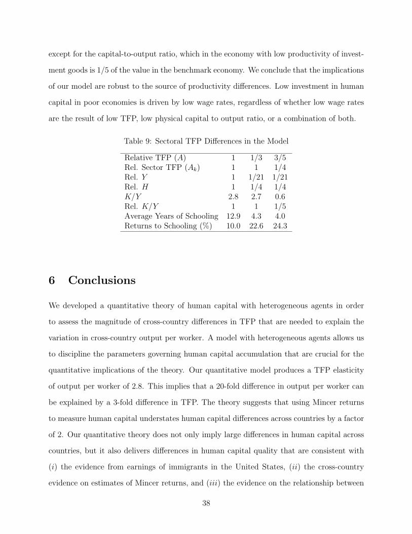
except for the capital-to-output ratio, which in the economy with low productivity of invest-

ment goods is 1/5 of the value in the benchmark economy. We conclude that the implications

of our model are robust to the source of productivity differences. Low investment in human

capital in poor economies is driven by low wage rates, regardless of whether low wage rates

are the result of low TFP, low physical capital to output ratio, or a combination of both.

Table 9: Sectoral TFP Differences in the Model

Relative TFP (A) 1 1/3 3/5Rel. Sector TFP (Ak) 1 1 1/4Rel. Y 1 1/21 1/21Rel. H 1 1/4 1/4K/Y 2.8 2.7 0.6Rel. K/Y 1 1 1/5Average Years of Schooling 12.9 4.3 4.0Returns to Schooling (%) 10.0 22.6 24.3

6 Conclusions

We developed a quantitative theory of human capital with heterogeneous agents in order

to assess the magnitude of cross-country differences in TFP that are needed to explain the

variation in cross-country output per worker. A model with heterogeneous agents allows us

to discipline the parameters governing human capital accumulation that are crucial for the

quantitative implications of the theory. Our quantitative model produces a TFP elasticity

of output per worker of 2.8. This implies that a 20-fold difference in output per worker can

be explained by a 3-fold difference in TFP. The theory suggests that using Mincer returns

to measure human capital understates human capital differences across countries by a factor

of 2. Our quantitative theory does not only imply large differences in human capital across

countries, but it also delivers differences in human capital quality that are consistent with

(i) the evidence from earnings of immigrants in the United States, (ii) the cross-country

evidence on estimates of Mincer returns, and (iii) the evidence on the relationship between

38

average years of schooling and per-capita income across countries. In our theory, countries

with low TFP also exhibit (relative to the benchmark economy) high inequality in earnings

and low intergenerational correlation of earnings. We leave for future work the quantitative

evaluation of how cross-country differences in TFP, fiscal policies, and the support for public

education affect economic inequality within countries.15

15There is abundant evidence in support of education and fiscal policies differences in developed and devel-oping countries. For instance, not only poor countries tend to devote less public resources to education, butalso they tend to support tertiary education disproportionally more than primary and secondary educationrelative to rich countries, with substantial distributional consequences.

39

References

Aiyagari, R. S. (1994): “Uninsured Idiosyncratic Risk and Aggregate Saving,” QuarterlyJournal of Economics, 109, 659–84.

Barro, R., and J.-W. Lee (1996): “International Measures of Schooling Years and School-ing Quality,” American Economic Review, 86(2), 218–23.

Bils, M., and P. Klenow (2000): “Does Schooling Cause Growth?,” American EconomicReview, 90(5), 1160–83.

Borjas, G. (1987): “Self-Selection and the Earnings of Immigrants,” American EconomicReview, 77(4), 531–53.

Davies, J., and J. Whalley (1989): “Taxes and Capital Formation: How Important isHuman Capital?,” Working Paper 2899, NBER.

Economic Report of the President (2004):. United States Government Printing Office, Wash-inghton.

Erosa, A., and T. Koreshkova (forthcoming): “Progressive Taxation in a DynasticModel of Human Capital,” Journal of Monetary Economics.

Fuster, L. (2000): “Capital Accumulation in an Economy with Dynasties and UncertainLifetimes,” Review of Economic Dynamics, 3(4).

Haveman, R., and B. Wolfe (1995): “The Determinants of Children’s Attainments: AReview of Methods and Findings,” Journal of Economic Literature, 33, 1829–78.

Hendricks, L. (2002): “How Important is Human Capital for Development? Evidencefrom Immigrant’s Earnings,” American Economic Review, 92(1), 198–219.

Heston, A., R. Summers, and B. Aten (2002): Penn World Table Version 6.1. Centerfor International Comparisons at the University of Pennsylvania (CICUP).

Hsieh, C., and P. Klenow (forthcoming): “Relative Prices and Relative Prosperity,”American Economic Review.

Jones, C. (1994): “Economic Growth and the Relative Price of Capital,” Journal of Mon-etary Economics, 34, 359–82.

Keane, M. P., and K. I. Wolpin (2001): “The Effects of Parental Transfers and Bor-rowing Constraints on Educational Attainment,” International Economic Review, 42(4),1051–1103.

Kendrick, J. W. (1976): The Formation and Stocks of Total Capital. Columbia UniversityPress (for the National Bureau of Economic Research), New York.

40

Klenow, P., and A. Rodriguez-Clare (1997): “The Neoclassical Revival in GrowthEconomics: Has It Gone Too Far?,” in NBER Macroeconomics Annual, ed. by B. S.Bernanke, and J. J. Rotemberg. MIT Press, Cambridge, MA.

Mankiw, N. G., D. Romer, and D. N. Weil (1992): “A Contribution to the Empiricsof Economic Growth,” Quarterly Journal of Economics, 107(2), 402–37.

Manuelli, R., and A. Seshadri (2005): “Human Capital and the Wealth of Nations,”mimeo.

Mulligan, C. B. (1997): Parental Priorities and Economic Inequality. University ofChicago Press, Chicago.

(1999): “Galton versus the Human Capital Approach to Inheritance,” Journal ofPolitical Economy, 107(6), S184–S224.

National Center for Health Statistics (2004): Health, United States, 2004 With Chartbookon Trends in the Health of Americans. Hyattsville, Maryland.

Neal, D. A., and W. R. Johnson (1996): “The Role of Premarket Factors in Black-WhiteWage Differences,” Journal of Political Economy, 104(5), 869–895.

Poterba, J. (1997): “The Estate Tax and After-Tax Investment Returns,” Working Paper6337, NBER.

Psacharopoulos, G. (1994): “Returns to Investment in Education: A Global Update,”World Development, 22, 1325–43.

Restuccia, D., and C. Urrutia (2001): “Relative Prices and Investment Rates,” Journalof Monetary Economics, 47(1), 93–121.

(2004): “Intergenerational Persistence of Earnings: The Role of Early and CollegeEducation,” American Economic Review, 94(5), 1354–78.

Solon, G. (1999): “Intergenerational Mobility in the Labor Market,” in Handbook of LaborEconomics, Vol. 3A, ed. by O. C. Ashenfelter, and D. Card, pp. 1761–1800. North-Holland,Amsterdam.

Statistical Abstract of the United States (1999):. U.S. Government Printing Office, Wash-ington, DC.

Stokey, N. L. (1998): “Shirtsleeves to Shirtsleeves: The Economics of Social Mobility,” inFrontiers of Research in Economic Theory: The Nancy L. Schwartz Memorial Lectures,1983-1997., ed. by D. P. Jacobs, E. Kalai, and M. I. Kamien, pp. 210–41. CambridgeUniversity Press, New York, NY.

Tauchen, G. (1986): “Finite State Markov Chain Approximations to Univariate and VectorAutoregressions,” Economics Letters, 20(2), 177–81.

41

Trostel, P. (1993): “The Effect of Taxation on Human Capital,” Journal of PoliticalEconomy, 101(2), 327–50.

U.S. Census Bureau (2004): Table P-32 Educational Attainment–Full-Time, Year-RoundWorkers 18 Years Old and Over by Mean Earnings, Age, and Sex: 1991 to 2003.<http://www.census.gov/hhes/www/income/histinc/p32.html>.

U.S. Department of Education (1996): Digest of Education Statistics. U.S. GovernmentPrinting Office, Washington, D.C.

U.S. Department of Education (2004): Digest of Education Statistics. U.S. GovernmentPrinting Office, Washington, D.C.

42

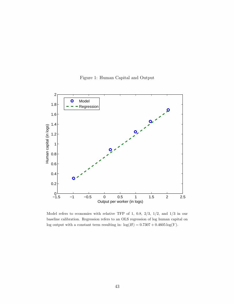
Figure 1: Human Capital and Output

−1.5 −1 −0.5 0 0.5 1 1.5 2 2.50

0.2

0.4

0.6

0.8

1

1.2

1.4

1.6

1.8

2

Output per worker (in logs)

Hum

an c

apita

l (in

logs

)

ModelRegression

Model refers to economies with relative TFP of 1, 0.8, 2/3, 1/2, and 1/3 in ourbaseline calibration. Regression refers to an OLS regression of log human capital onlog output with a constant term resulting in: log(H) = 0.7307 + 0.4605 log(Y ).

43

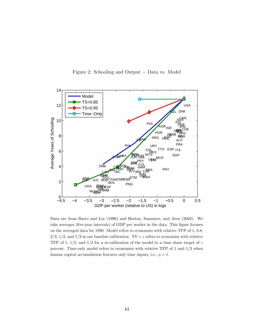
Figure 2: Schooling and Output − Data vs. Model

−4.5 −4 −3.5 −3 −2.5 −2 −1.5 −1 −0.5 0 0.50

2

4

6

8

10

12

14

GDP per worker (relative to US) in logs

Ave

rage

Yea

rs o

f Sch

oolin

g

DZA

BEN

BWACMR

CAF

COGEGY

GMB

GHAKENLSO

MWI

MLI

MUS

MOZNER

RWASEN

SLE

ZAF

TGOTUN

UGA

ZAR

ZMB

ZWE

BRB

CAN

CRI

DOMSLV

GTMHTI

HND

JAM

MEX

NIC

PAN

TTO

USA

ARG

BOLBRA

CHL

COL

ECUGUY

PRY

PER

URY

VEN

BGD

CHN

HKG

INDIDN

IRN

ISR JPN

JOR

KOR

MYS

NPL

PAK

PHL

SGPLKA

SYR

THA

AUT

BEL

CYP

DNK

FIN

FRA

GRC

HUNISLIRL

ITA

NLDNOR

POL

PRT

ESP

SWECHE

TUR

GBR

AUS

FJI

NZL

PNG

NAM

ModelTS=0.85TS=0.95Time−Only

Data are from Barro and Lee (1996) and Heston, Summers, and Aten (2002). Wetake averages (five-year intervals) of GDP per worker in the data. This figure focuseson the averaged data for 1990. Model refers to economies with relative TFP of 1, 0.8,2/3, 1/2, and 1/3 in our baseline calibration. TS = z refers to economies with relativeTFP of 1, 1/2, and 1/3 for a re-calibration of the model to a time share target of zpercent. Time-only model refers to economies with relative TFP of 1 and 1/3 whenhuman capital accumulation features only time inputs, i.e., η = 1.

44

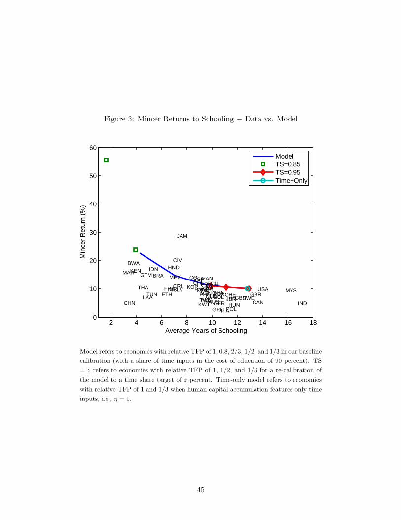
Figure 3: Mincer Returns to Schooling − Data vs. Model

2 4 6 8 10 12 14 16 180

10

20

30

40

50

60

Average Years of Schooling

Min

cer

Ret

urn

(%)

ARG

AUSBOL

BWA

BRA

CAN

CHL

CHN

COL

CRI

CIV

CYPDOM

ECUSLV

ETHFRA

GER

GHAGBR

GRC

GTMHND

HKGHUN IND

IDN

ISR

ITA

JAM

JPN

KEN

KOR

KWT

MYS

MEXMAR

NLDNIC PAK

PANPRY

PERPHL

POL

PRT

SGP

LKA SWECHE

TWN

THATUN GBR

USAURYVEN

ModelTS=0.85TS=0.95Time−Only

Model refers to economies with relative TFP of 1, 0.8, 2/3, 1/2, and 1/3 in our baselinecalibration (with a share of time inputs in the cost of education of 90 percent). TS= z refers to economies with relative TFP of 1, 1/2, and 1/3 for a re-calibration ofthe model to a time share target of z percent. Time-only model refers to economieswith relative TFP of 1 and 1/3 when human capital accumulation features only timeinputs, i.e., η = 1.

45

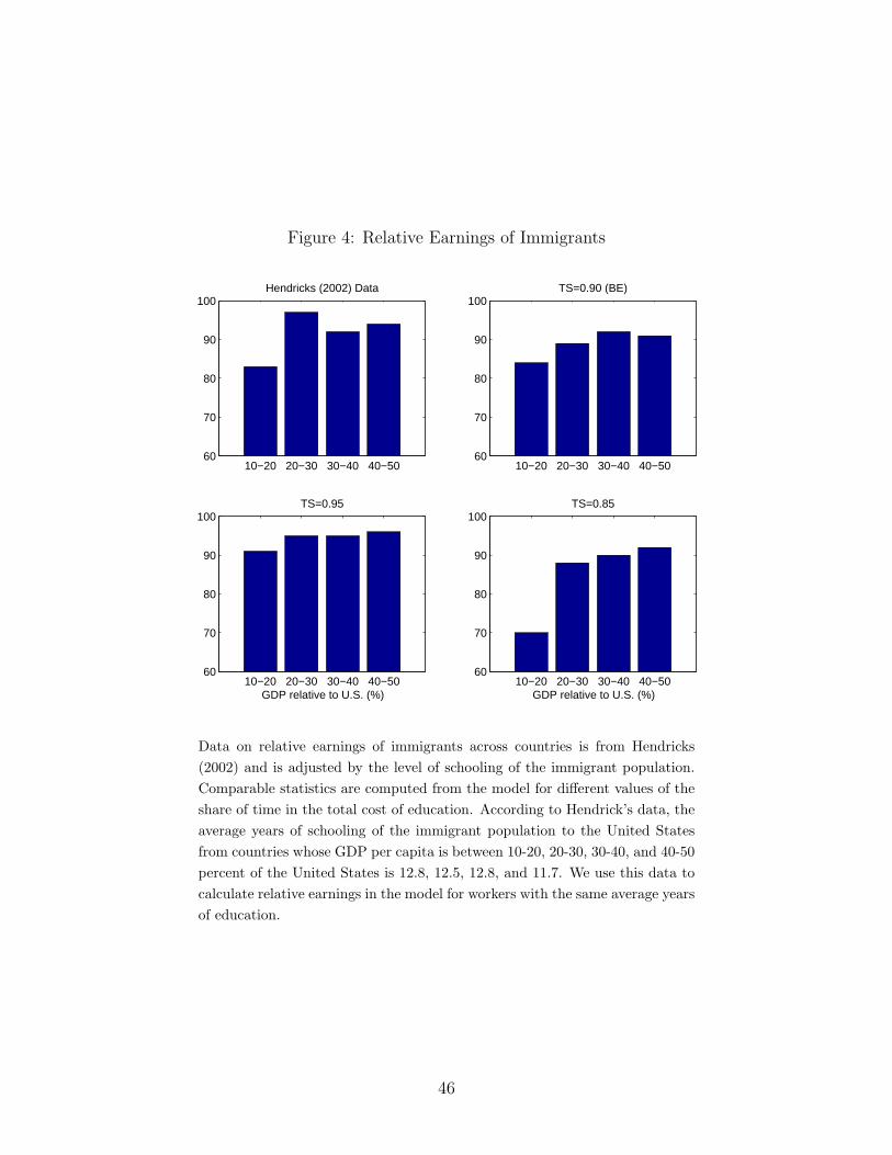
Figure 4: Relative Earnings of Immigrants

10−20 20−30 30−40 40−5060

70

80

90

100Hendricks (2002) Data

10−20 20−30 30−40 40−5060

70

80

90

100TS=0.90 (BE)

10−20 20−30 30−40 40−5060

70

80

90

100TS=0.95

GDP relative to U.S. (%)10−20 20−30 30−40 40−50

60

70

80

90

100TS=0.85

GDP relative to U.S. (%)

Data on relative earnings of immigrants across countries is from Hendricks(2002) and is adjusted by the level of schooling of the immigrant population.Comparable statistics are computed from the model for different values of theshare of time in the total cost of education. According to Hendrick’s data, theaverage years of schooling of the immigrant population to the United Statesfrom countries whose GDP per capita is between 10-20, 20-30, 30-40, and 40-50percent of the United States is 12.8, 12.5, 12.8, and 11.7. We use this data tocalculate relative earnings in the model for workers with the same average yearsof education.

46