Human capital theory 1. Introduction Basis for human capital theory: Worker productivity depends on either education or training, and these may be costly to provide. Human capital can be improved or enhanced in two main different ways: 1) Through formal education institutions 2) Through training on the job. Human capital formation can take two distinct, and economically crucial, forms: 1) General capital, implying that the skills/abilities acquired by

a worker has value in several (or possibly very many) firms. 2) Specific capital, implying that the skills and abilities have

value only in one particular firm, usually that firm which provides/makes possible the training.

Usually there is a connection between the issue of what institutions provide the training, and the form that the human capital takes. Formal education institutions usually provide only general capital, while most specific capital is provided by firms. In addition training provided by firms can be general. This has two separate, economically interesting, explanations. First, education institutions by their nature have an advantage in providing general capital, while firms have a comparative advantage in providing specific capital. Secondly, firms generally have incentive to provide specific training to their workers, but often much less general training. This will be illustrated below.

Acemoglu (2002) distinguishes between 5 views on ways of thinking about human capital, as follows:

1. The Becker view: Human capital is directly useful in the production process. May be termed the standard view, and the main one on which the human capital approach is based.

2. The Gardener view (after the psychologist Howard Gardener): Skills has many dimensions, such as mental and physical, and that different dimensions may be developed by different types of “training”.

3. The Schulz-Nelson-Phelps view: Human capital is mainly the capacity to adapt, in particular to changes in environment.

4. The Bowles-Gintis view: Human capital is the capacity to work in organizations, such as adapting to life in capitalist society. One main role of schools is to instill the “correct” ideology.

5. The Spence view: “Human capital” is basically given, and can be revealed through signals, and education or training can be such signals.

Essentially, 1-4 imply that human capital accumulation is valuable in the production process, albeit through different mechanisms. The Spence view is different, since here human capital accumulation does not occur. This will not be dealt with in these lectures.

One may next discuss what are the sources of human capital differences between individuals. Acemoglu (2002) distinguishes between six of these as follows:

1. Innate ability, which represents “genetic” differences between individuals, in their physical and mental characteristics correlated with work productivity.

2. Extent of schooling, whereby an individual can be expected to have higher productivity, generally or in some set of work activities, when the number of years of education increases.

3. School quality, representing the factor that a given education taken in different schools can increase an individual’s productivity differently.

4. Non-schooling investments, which represent effects on productivity from other factors than the schools, such as the amount of intellectual stimulus received by parents, the types of hobbies and acitivities exposed to during childhood and youth, and nutritional and health factors.

5. Training, representing factors affecting productivity once in a job.

6. Pre-labor market influences, which represent other stimuli from the social environment during early phases of life.

2. Optimal education length with perfectly general capital in continuous time We will start the analytic part with the simplest possible model of education choice in continuous time, where an education institution provides perfectly general human capital, the individual after the educational period is completed receives a constant wage equal to marginal product, and the individual pays the whole cost of education. Assume that the individual’s wage and productivity is constant after the educational period is completed. Define discounted lifetime income by R, given by

(1) ∫ ∫=

−−∞

=

−− +−−=+−=T

t

rTrT

Tt

rtrt erwe

rcdtwedtecR

0

)1()( ,

where the time from 0 to T is spent in education, and the rest of the time (until infinity) is spent working at a constant wage w. c is the educational cost per unit of time, and r the constant rate of interest (which may include a continuous and constant death probability). Assume that the worker’s productivity equals the wage (the worker receives the entire marginal product, and this product is the same in all firms). Moreover, this productivity increases with the length of the education, in deterministically and continuously, i.e., (2) .0'',0'),( <>= φφφ Tw This formulation of the problem implies that no improvement in the worker’s productivity nor wage is achieved after the formal educational period is completed.

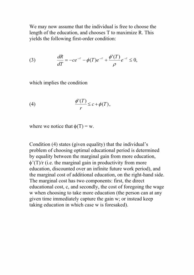
We may now assume that the individual is free to choose the length of the education, and chooses T to maximize R. This yields the following first-order condition:

(3) ,0)(')( ≤+−−= −−− rTrTrT eTeTcedTdR

ρφφ

which implies the condition

(4) )()(' TcrT φφ

+≤ ,

where we notice that φ(T) = w. Condition (4) states (given equality) that the individual’s problem of choosing optimal educational period is determined by equality between the marginal gain from more education, φ’(T)/r (i.e. the marginal gain in productivity from more education, discounted over an infinite future work period), and the marginal cost of additional education, on the right-hand side. The marginal cost has two components: first, the direct educational cost, c, and secondly, the cost of foregoing the wage w when choosing to take more education (the person can at any given time immediately capture the gain w; or instead keep taking education in which case w is foresaked).

Note that the educational cost c only incorporates direct educational costs (books, tuition, necessary travelling etc:) and not ordinary living expenses, which perhaps students identify with educational costs. The reason is that the latter expenses must be incurred regardless of whether taking education or not. An internal solution here arises only when equality can be achieved in (4). A possible case is φ’(0)/r < c + φ(0) for a particular individual. In this case the optimal educational choice is zero for this individual (we must here assume that an educational choice only is relevant beyond compulsory schooling). The net marginal return to education is then negative everywhere. The rule (4) is optimal both individually and socially, provided that there are no externalities, the worker always receives his or her full marginal product when working, and r is both the individual and social discount rate. (Note that r may incorporate a certain probability that the individual dies, at any given time, without loss of generality.) There are several reasons why optimality may not be achieved in practice, with fully general capital as assumed here. The main reasons can be summed up as follows: 1) The individual does not appropriate the whole marginal

return to education. This may happen for at least two main reasons, as will be elaborated in the following. First, the labor market need not be fully competitive, again for several different reasons. Secondly, taxation may put a wedge between social and private returns to education.

2) The individual does not pay the whole cost of education. In

most advanced countries all education, even at the highest level, is heavily subsidized.

3) Credit market imperfections. Observe that the solution (4) requires that individuals who are required (by their optimal solutions) to take long educations may at the same time be required to borrow heavily early in life, so as to pay back these loans later (since the optimal solution implies that labor income is received only after the education period is finished, and that the individual may need to finance a large educational expense early in life). This may require heavy borrowing early in life. But such borrowing may be difficult since lending institutions usually require collateral to give loans. Human capital is usually not allowable collateral in such contexts. (This again may be due to informational problems such as moral hazard and adverse selection, as will be elaborated in class). Thus necessary loans may either be denied, or interest on such loans may be excessively high. (Note again that higher private interest rates than the social rate of discount will distort the educational choice even when loans are not denied.)

Consider a simple case where we assume that the two factors 1) and 2) at the same time are at play, and that there are two “distortions”. First, the government taxes workers’ wages at a rate τ, and at the same time susidizes educational costs at a rate s. This implies that R and the educational choice can be characterized as follows (when we now assume an internal solution with respect to T): (5)

∫ ∫=

−−∞

=

−− −+−

−−=−+−−=

T

t

rTrT

Tt

rtrt ewecsdtwedtecspR0

)1()1()1()1())1(()(ρτ

ρτ

(6) wcsrT

)1()1()(')1(

τφτ

−+−=−

,

where we use the notation R(p) to indicate that we now are considering the private return to education, separate from the overall (or social) return R defined by (1).

We here easily derive two interesting results. First, consider the new first-order condition for workers, (6). We see that this is identical to the initial first-order condition (4) (which is also taken to be the social optimality condition) if and only if s= τ. Thus, the optimal solution is implemented if and only if the subsidy rate on educational expenditures equals the income tax rate. Then these two distortions, caused by each of the two instruments s and τ, will exactly cancel out. A requirement is of course that both s and τ are below unity. Secondly, consider the effect on net discounted government incomes from this individual (over the infinite future) of an increase in τ when s at the same time increases (so as to keep s = τ). Net government income can be written as (7) I = τR = [τ/(1-τ)]R(p). Note here that as long as s = τ, R is kept constant, since the educational choice of the individual is unaffected. Thus, obviously from (7), an increase in τ increases I proportionately. In the limit, when τ tends to unity, the entire net value is shifted to the government, while the individual is left with nothing. While this limit solution is extreme, it illustrates a principle at play here, namely that the government is able to extract part of workers’ rents from educational attainment, without distorting the educational choice, by taxing income and susidizing education at identical rates.

These results cannot generally be expected to hold in certain more general settings. We consider two such cases. First, the neutrality result when both s and τ are increased proportionately depends on all variables affecting the solution being observables. This need not always be the case. Assume as an example that there is an effort e(1) associated with education, and an effort e(2) associated with work. In this case one easily finds that the optimality condition with respect to T (given an internal solution) is characterized by

(8) ewcrT

++=)('φ ,

where e = e(1) – e(2) is the excess effort associated with education relative to work (which may be positive or negative). Optimality when taxes and subsidies are used is now possible only when also e is subsidized at a rate τ (i.e. the individual is paid a monetary equivalent of τe while taking education, which is a subsidy when e is positive and a tax if e is negative). The problem here is that e is likely not to be observable for any given individual (and is likely to vary between individuals). Note also that we are here assuming that the amount of leisure is the same for a person taking education as for a person working (there is then no leisure lost nor gained by choosing either of the two activities). Secondly, the work effort on the job in the work period, and thus productivity, may depend on the net wage (as e.g. in the model of efficiency wages). In such a case taxing wages will reduce productivities, and the above result will then also no longer hold.

Education in a simple model of matching We will now embed the above model of educational choice in a matching model of the Pissardies type. Consider a matching model where identical workers must choose educational length in the same way as in the model above. Assume bargaining as in the standard Pissarides model, with relative bargaining powers β and 1-β to the worker and individual firm respectively. Assume that the rate of matching is unaffected by the worker’s educational choice (in effect, all workers are matched at the same rate). Assume also that search for jobs can occur only after the worker’s educational period is completed. In line with previous analysis we may then assume that an individual, upon having achieved a desired level of education T, must enter the job market and start searching for possible vacant jobs. Search may thus not be performed while taking education. All jobs reward a given education equally. Finally as before, a gained job may be lost, at rate s, in which case new search is necessary. Denote the value of holding a job by V(E,T), and the value of being unemployed by V(U,T), both indexed by the amount of education taken by the worker at the time of entry into the labor market. V(U,T) is then given by the expression

(9) ),()(

)()(

),( TEVrr

bTUθλ

V θλθλ +

++

= .

The individual here always starts from the state of unemployment, and will then take the value of employment, V(E,T), as exogenous when deciding on further education. V(E,T) is given by

(10)

++

+++

+= b

srsTw

srr

rTE

)()(

)()(1),(

θλθλθλV ,

where we recognize explicitly that the wage w is a function of T. For reference we state the reduced-form expression for V(U,T), given by

(11) .)(

)()(

)(1),(

+++

+++

= bsrsrTw

srrTU

θλθλθλV

In these expressions b is interpreted as net leisure (gross leisure minus possible search costs while unemployed). Consider now first the case where workers are paid their full marginal products when working. We assume an internal solution to the educational problem, and that workers take λ(θ) as exogenously given. They will choose T according to the following rule (assuming again an internal solution with respect to T):

(12) ).,(),( TUrVcdTTUdV

=−

(12) is here derived in a manner equivalent to (4). (The left-hand side is the net return from continued education, while the right-hand side is the net return from finishing the education and start searching for a job.)

Using (9) and (10) to solve for rV(U;T) in terms of w and b, and inserting into (12) now yields the following general relationship (where we note that still λ = λ(θ)):

(13) bsrsrTw

srcTw

srr λλλ

λλ

+++

+++

=−++

)()('1 .

We see that (13) is a generalization of (4), in three separate ways: First, we have replaced the productivity function φ by a more general wage function. Secondly, the terms related to level and growth of wages,w and w’, have a smaller weight since wages are earned only with a lag after entering the labor market and then not for the entire labor market attachment period. Thirdly, net leisure b now counts as part of the value foregone by taking more education. A meaningful solution must here imply b < w(T). Consider here first the competitive case where w(T) ≡ φ(T). In this case the marginal wage gain φ’(T) must be greater than under the rule (4), which implies that T is smaller. This however does not automatically mean that T is suboptimal here. The fact that workers must go through unemployment before locating a job simply reduces the (private and social) return to education. If on the other hand the unemployment rate is inefficiently high, this here implies a tendency for education to also be inefficiently low.

Note that we also have assumed that the hiring rate of unemployed workers is independent of education. This may not be the case, and the solution is then different (Moen (1999) addresses this issue). Let us now instead assume that this choice is embedded in the Pissarides model of matching, job creation and wage formation. We there have previously derived the following equilibrium condition for job creation, adapted to the current model: (14) [φ(T)-w(T)]λ(θ) = (r+s)θk. We also have derived the following equilibrium wage equation: (15) w(T) = (1-β)b + β[φ(T) + θk]. (14) and (15) solve for w(T) and θ. φ(T) is here a given function, and k a given parameter. Workers’ educational choices thus determine their individual outputs, and all workers choose the same T. We are here not so interested in the explicit solution for θ, but rather in the solution for T as a function of the bargaining parameter β. Note here that each individual worker does not consider the change in θ nor in λ(θ) resulting from greater individual educational length (given that λ(θ) is not individualized and is the same for all workers). Thus w’(T) = βφ’(T) from (15).

Inserting from (15) in (13) then yields (16)

[ ] bsr

srkTsr

cTsrr λ

βλθφλ

λβφλ

λβ++−++

++++

=−++

)1()()('1 .

Setting φ ≡ w, we see when comparing (16) to (13) that now is lower when β < 1. This follows simply from the property of the Pissarides solution, that workers do not earn the entire marginal product.

So far we have ignored the possibility that workers may become employed directly from the educational state. In practice job offers may be forthcoming continuously also while taking education. In that case another issue arises, namely whether or not to take a given job offer, or to continue in school. This again raises the issue of two possible reservation productivities, namely one relevant for the choice of whether or not to take an offered job, and another (presumably higher) productivity at which one stops educating and enters unemployment. Consider now the value of staying in school, denoted by V(S,T). The return to this valu is given by

(17) [ ]dTTSdVTSVTEVcTSrV s

),(),(),(),( +−+−= λ

where λs is the job acquisition rate while taking education. The worker will be indifferent with respect to taking an offered job or not when taking education given that V(E,T) = V(S,T), which helps to define V(S,T). Moreover, for higher values of T, V(E,T) > V(S,T). This yields a lower bound for T called T0, up to which the worker will always take education. When no jobs are forthcoming, the worker will keep educating until V(S,T) = V(U,T). This helps to define a higher level of T, call it T1, beyond which the worker will never take education. Without going into details about this solution, it will imply that a certain fraction of workers have education levels over the whole interval [T0, T1], while another fraction of workers will have education at T1.

There are two obviously unrealistic aspect of this model. The first is the property that the rate at which job offers are forthcoming, either while undertaking education, or while unemployed, is independent of education. More realistically, these rates increase in education, since more educated workers typically are more profitable for employers (both under bargaining and under competition). Moen (1999) shows that when hiring probabilities increase in education, the propensity to undertake too little education, demonstrated under the models above, may disappear and we may instead have a “rat race” whereby education is overoptimal. The other way in which the model is unrealistic, is the assumption of identical workers, both in terms of actual productivities for given education, and in terms of the ease with which education can be acquired. The Spence signalling model, not dealt with in these lectures, here takes a diametrically opposite view by assuming that educational costs and productivities differ among individuals, while education as such does not enhance productivities. Education then becomes a pure signal of productivity, and not something inherently productive. In the context of the current model, one particularly unrealistic aspect is here that the longer one educates, the higher ones productivity as viewed by firms. Under a Spence sort of view it might rather be realistic to assume that individuals who complete a given education quickly are more productive than others. Then a particularly long educational period may serve as an adverse signal to employers.

3. On-the-job training The other form that human capital formation can take is as on-the-job (OTJ) training. Education is almost always general in the sense that it is useful in more than one (as a rule, very many) firm(s). OTJ training by contrast often has a much greater firm-specific component. It thus makes more sense to distinguish between possible general and firm specific components of the training received on the job. OTJ training is acquired in (at least) two distinct ways. First, workers may become more productive simply by working and interacting with other workers (learning by doing). Secondly, firms may design deliberate programs to train their workers. We will here concentrate on the latter, without denying that the former may be very important in practice. Consider first a standard “competitive” model. By this we here mean that a worker who is employed by a particular firm, is always paid his or her full marginal product in other firms, there is no unemployment nor frictions in any markets, and that workers may move freely between firms. The firm is assumed to set the worker’s wage. Assume that education is not important and does not affect productivities. OTJ training is however important.

Consider a particular worker who has productivity x before entering the firm in question. The worker may receive training at the start of the production period. Assume that after training, the worker’s productivity is given by (18) P = x + ψ(G) + π(S), where P is total productivity, ψ and π are components of productivity provided by general and specific training, and G and S are the overall costs of providing respectively general and specific training to the worker. Assume that ψ(0) = 0, ψ’ > 0, ψ’’ < 0, π(0) = 0, π’ > 0, π’’ < 0, and that the ψ and π function otherwise satisfy standard Inada conditions. The productivity of the worker after training, outside of the firm in question, is x + ψ(G). Thus since the firm sets the worker’s wage, and with no frictions and an otherwise competitive labor market, the wage earned by the worker outside of the firm in question is then also x + ψ(G). Consider the firm’s incentives to provide training in this case. The firm desires to maximize profit R, given by

(19 ) R = P – w – G(f) – S(f) = P - x - ψ(G(f)) – G(f) – S(f) = π(S(f)) – G(f) – S(f) with respect to G(f) and S(f), which denote the firm’s chosen levels of G and S, given that the worker sets these levels to zero. Note that w is determined by the best outside wage, in other firms. Obviously, G(f) will be set to zero, while S(f) will be determined by (20) π’(S(f)) = 1.

Consider now instead the worker’s decision to finance training of the two types himself, where G(w) and S(w) are the levels of training financed by the worker, in addition to any training financed by the firm. The net gain obtained by the worker can be written as (21) W = x + ψ(G(f)+G(w)) – G(w) – S(w) . Maximizing (20) with respect to G(w), and realizing that G(f) = 0, yields

(22) ψ’(G( w)) = 1. These results show that in a competitive labor market, the worker will (fully and efficiently) finance any general training, while the firm will (fully and efficiently) finance any specific training. This confirms Becker’s original analysis of general and specific training. Consider a simple extension of the above model, where the worker and firm bargain over the surplus in the one production period, and there is no mobility of labor between firms in the period (as in the implicit contract model considered in an earlier lecture). Set G = G(f) + G(w), S = S(f) + S(w). The net gain to the worker is then (23) w – G(w) – S(w), the net gain of the firm is (24) P – w – G(f) – S(f), where P = x + ψ(G) + π(S), as before from (17).

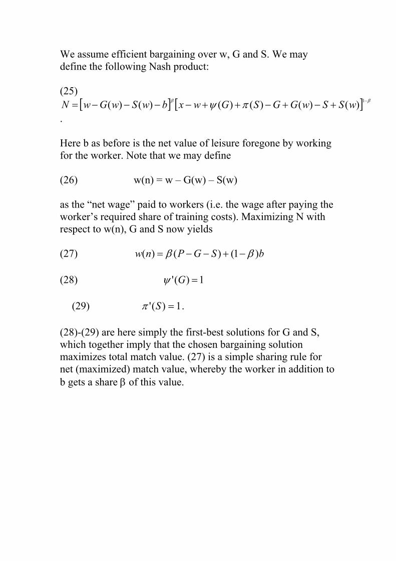
We assume efficient bargaining over w, G and S. We may define the following Nash product: (25)

[ ] [ ] ββ πψ −+−+−++−−−−= 1)()()()()()( wSSwGGSGwxbwSwGwN. Here b as before is the net value of leisure foregone by working for the worker. Note that we may define (26) w(n) = w – G(w) – S(w) as the “net wage” paid to workers (i.e. the wage after paying the worker’s required share of training costs). Maximizing N with respect to w(n), G and S now yields (27) bSGPnw )1()()( ββ −+−−= (28) 1)(' =Gψ

(29) 1)(' =Sπ . (28)-(29) are here simply the first-best solutions for G and S, which together imply that the chosen bargaining solution maximizes total match value. (27) is a simple sharing rule for net (maximized) match value, whereby the worker in addition to b gets a share β of this value.

Consider now instead a case where the firm is fully in charge of providing valuable OTJ training to workers. This may be a typical situation in practice, since individual workers may not be in a position to influence, and purchase, individual OTJ training. Assume also that training must be provided before the work period starts, such that the bargaining solution over wages will be struck after training has taken place. Since the worker will now pay no part of G nor S, we now have G = G(f), S = S(f). We will consider three versions of this problem, as follows: a) workers are not mobile in the period, b) workers may move to another firm in the period, and the

outside market is competitive, c) workers quit from the firm with exogenous probability δ ∈

(0,1), and stay with probability 1-δ, and the outside market is competitive.

Case a: Workers are not mobile In this case the firm, in deciding on G and S, realizes that the subsequent wage will be given by the rule

(30) w = βP + (1-β)b . Using expressions derived above, the firm now maximizes (31) R = P – w – G – S = x + (1-β)[x + ψ(G) + π(S) – b] – G - S with respect to G and S. This yields the solutions (32) (1-β)ψ’(G) = 1 (33) (1-β)π’(S) = 1. (32)-(33) imply that both G and S are underprovided by the firm. The obvious reason is that the worker appropriates a fraction β of the surplus created by the worker receiving additional training. This “bias” is however the same for general as for specific training. The no mobility case in a sense washes out the difference between G and S, since the worker now is not able to take advantage of the increase in G outside this particular firm. In the model, this increase thus works as if it were an increase in S. This resembles the Acemoglu and Pischke (1999) model of labor market imperfections, where a main point is that firms may get incentives to provide at least some general human capital to their workers, as a result of such imperfections.

Case b: Workers are fully mobile. In this case the worker will earn (34) w(m) = x + ψ(G) in the (competitive) outside market, and there is full labor mobility. Then w(m) will be the workers’ security level in the bargain with the firm, i.e., the wage will now be given by (35) w = βP + (1-β)[x + ψ(G)] = βπ(S) + x + ψ(G). Now the firm maximizes (36) R = P – w – G – S = (1-β) π(S) – G - S . Maximizing (36) with respect to G and S here obviously yields G = 0, and in addition the rule (33) for S. Thus G and S are here as in case a underprovided, but G (much) more than S. The firm here has no incentive whatsoever to provide general training, since it cannot capture any return to such training. We are here back to the basic Becker result with respect to G. Note however that this result is a bit “artificial”. We are namely assuming bargaining in the firm in question, but competitive allocation in “other firms”. A perhaps more consistent model would imply bargaining also in outside firms. Then the worker would not be able to recuperate the entire return to increased G in the outside market. This in turn would generally give the firm some incentive to invest in G.

Case c: Workers move with (exogenous) probability δ only. We now assume that workers may move, after training has taken place but before the production period starts, with given and exogenous probability δ ∈ (0,1). We assume as before that the firm cannot prevent the worker from quitting, nor force him to make any severance payment to the firm. Here the solution under a will result with probability 1-δ, while the firm will be left with nothing with probability δ. Then the firm’s expected return will be (37) ER = (1-δ)(1-β)[x + ψ(G) + π(S) – b] – G - S , since the costs G and S are incurred with certainty, while gross profits (as under case a) are earned only with probability 1-δ. Maximizing ER with respect to G and S yields (38) (1-δ)(1-β)ψ’(G) = 1 (39) (1-δ)(1-β)π’(S) = 1. Also in this case G and S are underprovided (marginally) in the same degree, but both are underprovided to a larger degree than under case a. As a consequence also, in this case G is overprovided and S underprovided relative to case b. Here the firm is reluctant to take on training since it knows the training will be wasted in many cases. An additional issue here arises when the probability δ depends on G and S (most likely, the dependence is positive for G and negative for S).

Note that under case a, the distinction between G and S is in a sense economically uninteresting, since both types of skills can be used only in the current firm (since there is no mobility whatsoever). In cases b and c, the distinction is economically interesting. In case b, potential mobility implies that G improves the threat point of the worker in the bargain with the firm. This has the effect that the firm provides no G whatsoever, as in Becker’s original model. In case c, the distinction between G and S is interesting through the effects training has in the case where the worker moves. Then only G affects productivity. This implies that although the rules (38) and (39) are identical, G is underprovided to a greater degree, since the social return to G is greater than the social return to S at the margin (since S has value only in the case where the worker stays, while G has value also when the worker moves). This version of the model resembles Acemoglu (1997), where a stressed point is that firms’ investments in human capital (specific or general) will be reaped in the future, by other firms whose identity is today unknown, and/or by current workers in such firms. This clearly reduces firms’ incentives to provide human capital. Case d: Endogenous mobility with encompassing bargaining An unrealistic aspect of the cases b and c is that the solution in “other firms” is taken to be competitive. But when there is all-encompassing bargaining throughout the economy, this is generally not the case. We will here assume such a case, and that the worker is free to move during the period, as under case b above. We will make the simplifying (but somewhat unrealistic) assumption that a worker may move just once and then to a firm which provides no specific capital. Then the outside utility of the worker during the bargaining phase will generally be lower than the outside worker productivity.

Consider again the case where the worker has bargaining parameter β versus all firms. The outside wage will then be (40) w(mb) = x + βψ(G) and (41) w = βP + (1-β)[x + βψ(G)] = x + β[π(S) + ψ(G)]. Now the firm maximizes (42) R = P – w – G – S = (1-β) [π(S) + ψ(G)] – G – S, Resulting in the first-order conditions (43) (1-β)ψ’(G) = 1 (44) (1-β)π’(S) = 1.

Human capital accumulation under outside-option bargaining So far we have assumed that when bargaining the parties’ security levels are their outside options. An alternative is to assume “outside option bargaining” as considered also under the Pissarides model above. This case is discussed in a paper by Kessler and Lülfesmann (2001). We then recall that whenever the “inside option” is valid, the bargaining solution yields the wage w(ob) given by (45) w(ob) = βP + (1-β)b = β[x + π(S) + ψ(G)] + (1-β)b. This will be the wage provided that it exceeds the outside option, defined by the productivity of the worker in the outside market, which under perfect mobility and competition in outside firms, is given by x + ψ(G). Thus the condition under which w(ob) will be the bargained wage is (46) βπ(S) + (1-β)b > (1-β)[x + ψ(G)]. When this condition holds, the firm in effect maximizes (31), resulting in the first-order conditions (32)-(33). As a consequence, the firm has incentives to provide general training in this case. Consider instead the case where the last condition does not hold. Then the wage will increase at the same rate as the increase in general productivity, leading to zero general productivity investments at the margin. On the other hand the wage will now be independent of S as long as the condition does not hold. The firm will then reap all the benefit at the margin, from an increase in S, thus invoking efficient investment in S. This implies that there is a complementarity between specific and general human capital in this case: When one is increased, the incentives generally increase to provide the other.

Minimum wages and human capital accumulation There are opposing views on the effects of mandatory minimum wages (enacted by law, or imposed by encompassing unions) on the incentives of workers and firms to accumulate human capital. Hashimoto (1982): Argues that firms try to counteract minimum wages (which push workers’ wages up beyond their marginal productivities) by reducing other benefits, and that OTJ training is such a benefit to be cut. Agell and Lommerud (1997): Argue that human capital formation for an “intermediate” group of workers may be affected positively by minimum wages imposed on a “primary” sector (their definition of a “secondary” sector is mainly nonmarket activity). The effect may be of two types. First, the worker may have greater incentives to take education in order to get access to the “primary” market (which requires a certain skill). Secondly, the firm’s incentives to provide training may increase, assuming bargaining between firm and worker over a net surplus (in excess of the minimum wage). For a low-skill group the effect may instead be negative as this group will be pushed out of the regular labor market by the minimum wage.

To illustrate the idea that minimum wages can increase education, and possibly make it more efficient when it is initially suboptimal, consider a simple model where a worker’s productivity is given by P = x + ψ(G) + π(S), in the firms in which they are engaged, as before, but let now G and S represent human capital investments by the worker and firm respectively. Initially, before a minimum wage is enacted, the worker and firm bargain over a net ex post surplus, P-b, where b as before is workers’ opportunity value of working, with relative bargaining strengths β and 1-β to the worker and firm. G and S must both be set before the wage is determined, and G is set “before” S. The solution for G, S and w are then given by (30) and the rules (32)-(33). In this case both G and S are underprovided, and both to the “same degree” (in terms of marginal products). Consider now alternatively that the government enacts a minimum wage M > b, below which the wage is not allowed to fall. Assume that firms never consider workers who arrive with initial productivity less than M. Then as a result of the bargaining, S is still determined by the same rule. Assume that initially, x + ψ(G0) < M. Then the worker will know that only if he takes more education than G0, will he get a job later. His choice will be GM such that x + ψ(GM) = M. It is now easy to see that whenever D = M - x - ψ(G0) is small, G will be set at a higher, and more efficient, level under minimum wages. When however D is large, it may be the case that G is now overprovided, and efficiency may fall.

Another aspect of this solution is that it, typically, redistributes surplus from the firm to the worker. This may be beneficial in cases with overestablishment of firms (where rents are dissipated through too high entry), but possibly not when there are “too few” firms at the outset, leading to unemployment. Then an additional consideration, in a social context and for the worker, is the probability of gaining employment as a function of the amount of education taken. Without analysing this in detail, we here get two opposing forces on G, namely a negative effect of the unemployment as such (the investment may be wasted as it may possibly not be used), and a positive effect of the possible increase in employment rate (my own probability of employment may go up when I take more education). The latter effect is similar to the rat race effect in Moen’s (1999) model, which may lead to overinvestment in education.

References: Acemoglu, D. (2002), Lecture notes for graduate labor economics, MIT (lecture notes can downloaded from Acemoglu’s home page, http://econ-www.mit.edu/faculty/acemoglu/files/courses/labornoteswithpics.pdf) Acemoglu, D. (1997), Training and innovation in a competitive labor market. Review of Economic Studies, 64, 445-464. Acemoglu, D. and Pischke, J. S. (1999), Journal of Political Economy Agell, J. and Lommerud, K. E. (1997), Minimum wages and the incentives for skill formation. Journal of Public Economics, 64, 25-40. Hashimoto, M. (1982), Minimum wage effects on training on the job. American Economic Review, 72, 1070-1087. Kessler, A. S. and Lülfesmann, C. (2001), The theory of human capital revisited: On the interaction of general and specific capital. Working paper, University of Bonn. Moen, E. (1999), Education, ranking, and competition for jobs. Journal of Labor Economics, 17, 694-723.