A Quantitative Theory of Tax Evasion and Informality∗

Jose Joaquın Lopez†

University of Memphis

March 1, 2016

Abstract

I study how heterogeneous establishments optimally select themselves into informality, tax

compliance, and formal tax evasion, through the lens of a general equilibrium model. I

calibrate the model to match key moments of the employment size distribution in Mexico,

as well as some aggregate moments. In equilibrium, tax revenues rely on medium-sized

firms, which are scarce. Eliminating informality (formal tax evasion) increases tax collection

by 80 (68) percent. As the economy develops, the informal sector shrinks, while the tax-

evading sector expands, thus limiting potential collection. If lower informality is a byproduct

of development, and not vice versa, a solid tax base can be achieved by fiscal authorities

effectively via enforcement on formal, tax-evading firms.

Keywords: Tax evasion, formal sector, informality, enforcement, rent seeking, firm hetero-

geneity.

JEL Classification Codes: H26, H32, K42, L26, O17, O43, O47.

∗I am extremely grateful to my advisor, Nancy Stokey, for her guidance and support. I received helpfulcomments from Jon Anderson, Matthew J. Cushing, Julio C. Leal-Ordonez, Bob Lucas, Fernando Perez,Erwan Quintin, Andrei Shleifer, Bill Smith, Sebastian Sotelo, and seminar participants at Banco de Mexico,the Chicago Fed, and the University of Nebraska, Lincoln. This paper greatly benefited from a conversationwith Paco Buera, to whom I am grateful. My gratitude to Natalia Volkow and the Censos Economicos areaat INEGI for their help with the data. The statistics used in this study have been reviewed by Mexico’sINEGI to ensure no confidential information is disclosed. This work was supported by a grant from theFogelman College of Business & Economics at the University of Memphis. All errors are mine.†Department of Economics, Fogelman College of Business & Economics, University of Memphis, e-mail:

jjlopez@memphis.edu.

1

1 Introduction

Informality as well as tax evasion by formal firms are pervasive in developing countries.

Many firms choose to remain small and avoid taxes and regulations altogether, whereas

others are able to reduce their tax burden through lawyers, accountants, and bribes or

other forms of corruption. While there are numerous studies that model informality and

its aggregate effects, the rent-seeking activities undertaken by many formal firms are largely

ignored in traditional theories of production. I show how firms optimally select themselves

into informality, tax compliance, and formal tax evasion, according to their productivity and

the institutional environment.

Tax evasion and tax avoidance have always existed: from wealthy Romans in the third

century burying their jewelry to avoid the luxury tax, to eighteen-century English homeown-

ers who bricked up their fireplaces to escape notice from the hearth tax collector (Slemrod,

2007, on Webber and Wildavsky, 1986), to Apple’s multi-billion dollar accounts in offshore

tax havens.1 Even in the modern-day U.S., Slemrod (2007) cites an IRS estimate of 17

percent for the noncompliance rate of the corporate income tax in 2001. The World Bank

Enterprise Survey estimates that 54% of companies across 135 developing countries do not

report all income tax to authorities, while Artavanis, et.al. (2015) report a not-so-small

figure of 36% for Europe.

Evidently, these tax-evading activities are not costless—the wealthy Romans and the

English homeowners spent some of their valuable time digging and laying bricks, while

Apple undoubtedly hires many skilled accountants and lawyers to devise and execute their

tax-minimizing strategies. Also implied in these anecdotes is the notion that higher stakes

usually command higher efforts, as hiding personal jewelry certainly requires less resources

than avoiding a multi-billion dollar tax bill. The idea that larger, more productive firms find

it more attractive to engage in “defensive” rent seeking is also recognized by Tullock (1992).

This paper makes four contributions. First, I show how agents optimally choose the

tax-evading efforts just described as a function of their productivity, market prices, and the

institutional environment. Specifically, I consider an environment where formal firms can

reduce their fiscal burden by spending resources—either legally or illegally. This formulation

is not particular to developing countries, and can be thought of as a quantitative framework

to think about the ideas first posed by Krueger (1974). The degree of rent seeking observed

in the model economy depends on the stringency of the tax system, as well as on the level of

enforcement and statutory provisions that allow firms to reduce their fiscal outlay, i.e. the

returns to firms’ tax-evading efforts. The theory predicts that larger, more productive firms

1See “Apple’s Web of Tax Shelters Saved It Billions, Panel Finds,” The New York Times, May 20, 2013.

2

spend more resources in tax-avoiding/evading activities, and thus face a lower tax burden.

Second, I apply the theory to the specific case of business income taxes, and show how

the mixture of formal tax-evading, formal tax-compliant, and informal firms is determined in

equilibrium. To this end, I develop a model where individuals with idiosyncratic managerial

abilities face the choice of becoming formal entrepreneurs, informal entrepreneurs, or workers.

Informal entrepreneurs avoid paying taxes by staying small, while formal entrepreneurs have

the choice of complying with the tax code, or spending resources to reduce their fiscal outlay.

The coexistence of small informal firms that do not pay taxes and large formal tax-evading

firms results in an effective tax schedule that relies on medium-sized firms. This result links

the evidence on the “missing middle” of the distribution of firm sizes in developing countries

to a low capacity of the state to generate tax revenues—which is another common feature

of many developing countries.

Third, I calibrate the model to the Mexican economy—where informal firms employ

34 percent of workers, and tax evasion by formal firms is estimated at 37 percent of tax

collection. The model does well at replicating some non-targeted moments of the data,

including some limited evidence on firm-level effective income tax rates. I then consider the

effects of three counterfactual policy experiments: 1) improved partial enforcement, 2) full

enforcement, and 3) changes in the statutory tax rate. I find that eliminating informality

(tax evasion by formal firms) increases tax revenues as a percentage of GDP by 80 (68)

percent. TFP, investment and output respond positively to partial and full reductions in

informality, but remain unaffected by enforcement on formal firms. I find that both partial

and complete reductions in informality increase the amount of rent seeking in the economy.

Last, the Laffer curve generated by the model suggests that Mexico’s recent income tax rates

have been near the revenue-maximizing value, and thus the state’s capacity to raise revenues

is unlikely to improve via further changes to these rates.

Finally, I explore the effects of economic development on the equilibrium mixture of firms,

tax revenues, as well as the amount of tax evasion in the economy. As the economy grows,

for given taxes and enforcement parameters, the informal sector shrinks, and eventually

disappears. The share of formal, tax evading firms, however, continues to grow with the

economy, limiting the state’s capacity to raise tax revenues even as the economy prospers.

The last result provides a rationale for the existence of developed countries with high levels

of tax evasion and/or avoidance, and helps explain the rise of occupations such as accounting

and law as economies develop. The findings suggests that, to the extent that lower informality

is a byproduct of development, and not vice versa, a solid tax base can be achieved by fiscal

authorities more effectively via enforcement on formal, tax-evading firms.

Clearly, there are other aspects of formal tax evasion and tax avoidance that deserve

3

attention. The feature of tax evasion often highlighted in the literature is the probability

of being caught by the tax authorities, which usually comes with a punishment, as in the

seminal work of Allingham and Sandmo (1972). In this paper, I focus on a largely unexplored

dimension of firm-level tax evasion and tax avoidance, namely, that they are costly activities

optimally chosen by firms, much like any other productive input, and that they reflect both

loop holes in the tax code, as well as the state’s capacity to enforce it. My treatment of tax

avoidance and tax evasion is similar to Mayshar (1991), and Slemrod (2001), who study the

partial equilibrium decision of a utility-maximizing individual taxpayer with access to a “tax

technology” that allows him to exert labor effort to reduce his tax burden. Acemoglu (2005)

and Piketty, et.al. (2014) also consider economies where tax sheltering is costly, although

their focus is on a different set of issues.

My treatment of informality borrows heavily from Leal-Ordonez (2014), who studies the

aggregate effects of informality due to incomplete tax enforcement at the extensive margin.

Additionally, I analyze the effects of incomplete tax enforcement at the intensive margin, in

the same spirit as Ulyssea (2015), who considers an economy where firms can be informal

either by not registering their business, or by hiring workers “off the books.”. Even though

I consider ways in which firms avoid taxes different than outsourcing of employees, to the

extent that outsourcing is a costly activity that brings the firm some tax benefits, Ulyssea’s

core idea is implicit in my formulation.

2 A model economy

2.1 Entrepreneurial choice, tax evasion and informality

There is a representative household populated by a unit continuum of members. En-

trepreneurial ability is distributed over the household members according to some distribu-

tion F (Z), with bounded support [ZL, ZH ], and pdf f(Z); with ZL ≥ 0. Agents can choose

to become formal entrepreneurs, informal entrepreneurs, or workers. Formal entrepreneurs

have, in turn, the choice of being fully compliant with the tax code, or to engage in costly

rent-seeking activities to reduce their tax burden.

If agents choose to become entrepreneurs—irrespective of the type—they can operate a

diminishing-returns to scale technology that utilizes capital and labor as inputs to produce

a homogeneous good, as in Lucas (1978). Output by an entrepreneur of ability Z is given

by

Y = Z1−θ (KαN1−α)θ , (1)

4

where K and N are the amount of capital and the number of workers hired by the firm,

α ∈ (0, 1) is the share of capital and θ ∈ (0, 1) measures the span of control. If the agent

chooses to become a worker, he earns a wage w.

Firms face a statutory tax on profits τ0. Formal firms can choose to comply with the

statutory tax, or to pay bribes or hire expediters to reduce their tax liability. I call these

rent-seeking expenditures B. In the derivations below, I assume the tax-evasion technology

faced by a formal firm takes the following functional form:

τ = τ0 exp (−φB) ,

where τ is the effective tax rate, and φ ≥ 0 measures the returns to the formal entrepreneur’s

rent-seeking efforts. The parameter φ represents both the level of enforcement on formal

firms, as well as the statutory provisions in the tax code which allow firms to reduce their

fiscal burden. Exploiting these provisions, in turn, usually requires hiring an expediter. In

general, the pair (τ0, φ) can vary across countries, across sectors, or even across firms. In

what follows I assume τ0 and φ are the same for all firms.

If the entrepreneur chooses to evade taxes, his problem is then to choose (KE, NE, B) ,

given Z, τ0, φ and factor prices (w, r) , to maximize profits,

ΠE(Z) ≡ maxKE ,NE ,B

(1− τ0e−φB

) [Z1−θ (Kα

EN1−αE

)θ − rKE − wNE

]−B,

subject to B ≥ 0.

The optimal choices by the entrepreneur are

KE(Z) = Z

[αθ

rκ−θ(1−α)

] 11−θ

, (2)

NE(Z) = Z

[(1− α)θ

wκθα] 1

1−θ

, (3)

B(Z, φ) =1

φln(τ0φ[Z1−θ (Kα

EN1−αE

)θ − rKE − wNE

]), (4)

Where

κ ≡ KE

NE

=

(α

1− α

)w

r

is the capital-labor ratio common to all formal firms. Notice that the input choices are

independent of the choice of rent-seeking expenditures and the effective tax rate. Therefore,

5

neither the statutory tax, or the possibility of reducing it distort the optimal choices of

capital and labor. In this economy, larger, more productive firms spend more in rent seeking

and thus have a lower tax burden.

In general, tax evasion is a gamble not explicitly considered in this formulation. However,

the risky aspect of tax evasion can be presented in this framework if, as explained by Mayshar

(1991), one defines B as the payment which generates the same expected profit loss as the

extra risk an evading firm takes on, for given expected tax payments. In what follows I use

the terms “evasion” and “avoidance” interchangeably.

Let Ψ(w, r) be defined as

Ψ(w, r) = (1− θ)(θα

r

) αθ1−θ(θ(1− α)

w

) (1−α)θ1−θ

(5)

The profits of the tax-evading entrepreneur are then given by

ΠE(Z) = ZΨ(w, r)− 1

φ[1 + log (τ0φZΨ(w, r))] . (6)

Entrepreneurs who chose to comply with the tax code solve the following problem

ΠC(Z) ≡ maxKC ,NC

(1− τ0)[Z1−θ (Kα

CN1−αC

)θ − rKC − wNC

],

Their input choices are

KC(Z) = Z

[αθ

rκ−θ(1−α)

] 11−θ

, (7)

NC(Z) = Z

[(1− α)θ

wκθα] 1

1−θ

, (8)

with profits

ΠC(Z) = (1− τ0)ZΨ(w, r). (9)

I model informality as in Leal-Ordonez (2014). Informal entrepreneurs do not pay any

taxes. They are able to do so by staying small. I assume that the government has the ability

to detect any firm with a capital stock greater than some D > 0. In the case of detection,

the firm is shut down and the entrepreneur earns zero profits. Therefore, the greater D,

the lower the ability of the government to detect informal firms. This threshold strategy is

consistent with optimal tax enforcement by a government with low resources that is able to

6

observe input choices by firms, which are in turn signals of the entrepreneur’s productivity,

as shown by Bigio and Zilberman (2010).

Thus, we can write the problem solved by informal entrepreneurs as follows,

ΠI(Z) ≡ maxKI ,NI

Z1−θ (KαI N

1−αI

)θ − rKI − wNI ,

subject to

KI ≤ D.

Let µ(Z) denote the multiplier on the size constraint—the shadow cost of informality.

Highly productive entrepreneurs will face a higher µ(Z), while unproductive entrepreneurs

may not be bound by the size constraint at all, thus facing a multiplier equal to zero. As

long as there is a positive measure of informal entrepreneurs for which µ(Z) > 0, there will

be aggregate productivity losses from informality.

The input choices of informal firms are

KI(Z) = Z

[αθ

r + µ(Z)κ(Z)−θ(1−α)

] 11−θ

, (10)

NI(Z) = Z

[(1− α)θ

wκ(Z)θα

] 11−θ

, (11)

where

κ(Z) =

(α

1− α

)w

r + µ(Z)

is the capital-labor ratio, which varies across informal firms. Firms that face a higher

shadow cost of informality have a lower capital-labor ratio.

The profits of informal firms are then,

ΠI(Z) = ω(Z)ZΨ(w, r). (12)

where ω(Z) =(

rr+µ(Z)

) αθ1−θ

is the profit wedge caused by firms’ choice of staying small

to avoid paying taxes, resulting in a fraction 1 − ω(Z) of profits being lost—an implicit

informality tax. Figure 1 shows ω(Z). As Z increases, it becomes less and less profitable to

operate as an informal firm.

With this notion in hand, notice that an entrepreneur’s pre-tax (and pre-tax-evasion

expenditures when applicable) profits are given by ZΨ(w, r), regardless of firm type. The

7

00

1

Z

t(Z)

Figure 1: Profit wedge due to informality.

differences in net profits across firm types, then, arise from differences in the cost of doing

business: informal firms pay an implicit informality tax, formal compliant firms pay the

statutory tax, while formal tax-evading firms pay a combination of taxes and tax-evasion

expenditures.

Lemma 1 There exists a unique value ZE, such that if Z > ZE, formal firms choose to

evade taxes. This value is given by ZE = [φτ0Ψ(w, r)]−1.

All proofs are in the appendix. The equilibrium cutoff ZE is decreasing in φ and τ0,

since as both increase it becomes more profitable to spend resources to evade taxes, so more

firms engage in formal tax evasion. It is increasing in w and r, a property helpful to explain

general equilibrium effects in the next sections.

In the same spirit as the choice of tax evasion by formal firms, the choice of informality

will be characterized by a threshold for productivity, which I call ZI . Entrepreneurs with

ability below ZI will be informal, while those with Z ≥ ZI will be formal. If ZI > ZE, there

are no formal firms that are fully complaint with the tax code: only informal and tax-evading

formal firms co-exist. The mixture of firm types will depend on the policy parameters τ0, φ,

and D.

Lemma 2 If there is a productivity level ZP > 0, such that ω(ZP ) > (1− τ0), then there

exists a unique value ZI ≥ ZP , such that ΠI(ZI) = max{ΠC(ZI),ΠE(ZI)}. If Z ≤ ZI , the

entrepreneur chooses to be informal.

8

Agents observe their productivity draw Z, and then choose to either become an en-

trepreneur or a worker, whichever gives them the highest earnings. Their problem is then

V (Z) = max {Π∗(Z;w, r, φ, τ0, D), w} ,

Where Π∗(Z;w, r, φ, τ0, D) = max {ΠI(Z),ΠC(Z),ΠF (Z)}.

Lemma 3 There exists a unique value ZW such that V (ZW ) = Π∗(ZW ;w, r, φ, τ0, D) = w.

If Z < ZW , the agent chooses to become a worker.

2.2 Accumulation

The household derives utility from consumption streams only, and discounts the future

at a rate β ∈ (0, 1). It is endowed with an initial capital stock K0 > 0, as well as a unit of

time each period, which is supplied inelastically. The household consumes and accumulates

capital so as to maximize lifetime utility,

maxCt,Kt+1

∞∑t=0

βtu(Ct),

subject to

Ct +Kt+1 ≤ (1− δ + rt)Kt +

∫ ZH

ZL

V (Z)dF (Z) + Tt,

where∫ ZHZL

V (Z)dF (Z) are the aggregate household earnings, and Tt is a lump-sum trans-

fer from the government. The function u(·) is strictly increasing and strictly concave and

satisfies Inada conditions. At the steady state, the Euler equation provides the standard

result for the rental rate of capital

r =1

β− (1− δ).

2.3 Government

The government collects revenues Rt from taxes and informality penalties. Since in

equilibrium no informal firm is caught, all revenues come from tax collection. I assume the

government runs a period-by-period balanced budget, so Rt = Tt, all t. Revenues from

formal, compliant firms—when these exist—are given by

RC =

∫ ZE

ZI

τ0Ψ(w, r)ZdF (Z) = τ0Ψ(w, r) [F (ZE)− F (ZI)].

9

The effective tax paid by formal, tax-evading firms is given by

τ(Z) = τ0 exp [−φB(Z)] =1

φΨ(w, r)Z.

Notice that it does not depend on τ0. Then, when ZE > ZI revenues from formal,

tax-evading firms are

RE =

∫ ZH

ZE

τ(Z)Ψ(w, r)ZdF (Z) =1

φ[F (ZH)− F (ZE)].

Total revenues are then R = RC + RE. When ZE < ZI , there are no formal firms that

comply with the tax code, and so all revenues come from tax-evading firms,

R = RE =1

φ[F (ZH)− F (ZI)].

2.4 Equilibrium

A steady-state competitive equilibrium consists of constant input prices (w, r), constant

aggregate levels of consumption (C) and capital (K), an occupational choice cutoff ZW ,

and firm-type choice cutoffs {ZI , ZE} with their corresponding collections of input policies

{K∗(Z;w, r), N∗(Z;w, r), B(Z;w, r)} indexed by Z, such that:

i) the representative household problem is solved: r = 1/β − (1− δ),ii) the firm-type choices and their respective input policies maximize profits, taking (w, r)

as given,

iii) the occupational choices maximize household earnings, taking (w, r) as given,

iv) the labor, capital, and goods markets clear, and

∫ ZW

ZL

dF (Z) =

∫ ZH

ZW

N∗(Z;w, r)dF (Z), (13)

K =

∫ ZH

ZW

K∗(Z;w, r)dF (Z), (14)

C + δK =

∫ ZH

ZW

Y ∗(Z)dF (Z)−∫ ZH

max{ZE ,ZI}B(Z;w, r)dF (Z), (15)

v) the government budget is balanced.

Rt ≡∫ ZL

ZW

τ ∗(Z)Π∗(Z) = Tt.

10

1

w

workers formal tax-compliant formal tax-evadinginformal

Z1-θZE1-θZI

1-θZ01-θZW

1-θ

informal unconstrained(μ(Z) =0)

0

ΠI(Z)

ΠC

(Z)

ΠE

(Z)

Figure 2: Equilibrium occupational and firm type choice—Case I: ZI < ZE.

Where K∗(Z;w, r), N∗(Z;w, r), Y ∗(Z;w, r), and τ ∗(Z) correspond to the firm-type

choice Π∗(Z) = max {ΠI(Z),ΠC(Z),ΠF (Z)}.The rental rate of capital is determined by the inter-temporal problem of the household.

The thresholds—whose existence was determined in the previous section—and the wage rate

are determined jointly through the labor market clearing condition. Notice that the left-hand

side of (13) is the household’s labor supply, which is strictly increasing in w (since ZW is

increasing in w), while the right-hand side is the aggregate labor demand, which strictly

decreasing in w (since ZW is increasing in w and N∗(Z;w, r) is decreasing in w). Therefore,

if an equilibrium exists, it is unique. In fact, since N∗(Z;w, r) → 0 as w → ∞, and

N∗(Z;w, r)→∞ as w → 0, and labor supply is zero when w = 0, existence is guaranteed.

In Figure 2, I show the equilibrium determination of occupational, and firm type choices

for a case in which ZE > ZI . The figure plots the equilibrium profits for each type of firm,

as well as the wage rate, as a function of rescaled productivities Z1−θ.2 The lower bound

for productivities is set at one. Agents with productivities between one and ZW choose to

become workers, whereas those with productivities greater than ZW but less than ZI choose

to operate informal firms. Informal entrepreneurs with an ability between ZW and Z0 are

unconstrained by the detection threshold, and thus face a shadow cost of informality, µ(Z),

of zero, while for those with abilities between Z0 and ZE, µ(Z) > 0. Entrepreneurs with

abilities between ZI and ZE choose to comply with the statutory tax rate, whereas those

with abilities greater than ZE engage in costly tax evasion.

2The rescaling is just for ease of display purposes.

11

2.5 TFP losses from informality

Consider the centralized problem of allocating aggregate stocks of capital and labor across

firms distributed over the interval [ZW , ZH ] according to some c.d.f. F (·), so as to maximize

total output

max{K(Z),N(Z)}

Y =

∫ ZH

ZW

Z1−θ(K(Z)αN(Z)1−α)θdF (Z),

subject to

K =

∫ ZH

ZW

K(Z)dF (Z),

N =

∫ ZH

ZW

N(Z)dF (Z).

Let Z =∫ ZHZW

ZdF (Z). In an economy without informality, capital and labor are allocated

so as to equalize returns to each factor across firms, which satisfies, for all Z,

K(Z) =Z

ZK,

N(Z) =Z

ZN.

Aggregate output is then equal to

Y = TFP F (KαN1−α)θ,

where

TFP F =Y

(KαN1−α)θ= Z1−θ.

Now consider an economy where there are some informal firms. The labor and capital

allocations of informal firms in this case are

K(Z) = ωK(Z)Z

ZK,

N(Z) = ωN(Z)Z

ZN.

12

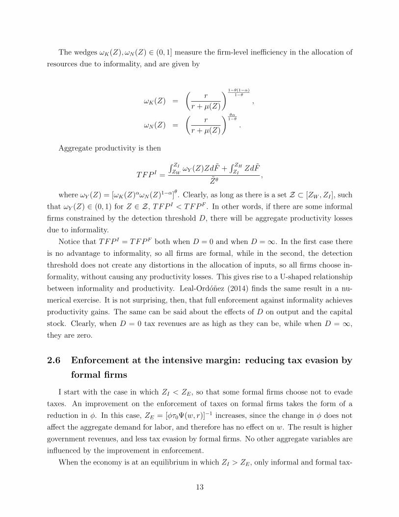
The wedges ωK(Z), ωN(Z) ∈ (0, 1] measure the firm-level inefficiency in the allocation of

resources due to informality, and are given by

ωK(Z) =

(r

r + µ(Z)

) 1−θ(1−α)1−θ

,

ωN(Z) =

(r

r + µ(Z)

) θα1−θ

.

Aggregate productivity is then

TFP I =

∫ ZIZW

ωY (Z)ZdF +∫ ZHZI

ZdF

Zθ,

where ωY (Z) = [ωK(Z)αωN(Z)1−α]θ. Clearly, as long as there is a set Z ⊂ [ZW , ZI ], such

that ωY (Z) ∈ (0, 1) for Z ∈ Z, TFP I < TFP F . In other words, if there are some informal

firms constrained by the detection threshold D, there will be aggregate productivity losses

due to informality.

Notice that TFP I = TFP F both when D = 0 and when D =∞. In the first case there

is no advantage to informality, so all firms are formal, while in the second, the detection

threshold does not create any distortions in the allocation of inputs, so all firms choose in-

formality, without causing any productivity losses. This gives rise to a U-shaped relationship

between informality and productivity. Leal-Ordonez (2014) finds the same result in a nu-

merical exercise. It is not surprising, then, that full enforcement against informality achieves

productivity gains. The same can be said about the effects of D on output and the capital

stock. Clearly, when D = 0 tax revenues are as high as they can be, while when D = ∞,

they are zero.

2.6 Enforcement at the intensive margin: reducing tax evasion by

formal firms

I start with the case in which ZI < ZE, so that some formal firms choose not to evade

taxes. An improvement on the enforcement of taxes on formal firms takes the form of a

reduction in φ. In this case, ZE = [φτ0Ψ(w, r)]−1 increases, since the change in φ does not

affect the aggregate demand for labor, and therefore has no effect on w. The result is higher

government revenues, and less tax evasion by formal firms. No other aggregate variables are

influenced by the improvement in enforcement.

When the economy is at an equilibrium in which ZI > ZE, only informal and formal tax-

13

evading firms operate. In this case, a decrease in φ will increase the informality cutoff ZI ,

increasing the size of the informal sector. To the extent that there were some constrained

informal firms operating before the change, the marginal firms coming into the informal

sector as a result of the change in φ will be constrained, which will result in lower TFP and

a lower aggregate capital stock.

The effect on government revenues is not as clear: on one hand, firms that were paying

some taxes before the change will not pay any taxes, since they will move to the informal

sector. On the other hand, the remaining tax-evading firms will face a stronger enforcement,

which increases the revenue collected from them. The total impact on revenues depends on

which effect dominates.

Ultimately, because changes in either margin of enforcement affect the equilibrium pro-

ductivity thresholds for firm type and occupational choices, their aggregate effects depend

on the distribution of productivities, F (·). Thus, to move forward in the discussion of the

effects of enforcement, we need to impose a parametric structure and assign parameter values

that closely match some aspects of a real economy.

3 Parameterization and calibration

I follow the vast literature on firm-size distributions starting with Axtell (2001), and

assume that productivities are distributed according to a Pareto distribution. In particular,

I assume that the rescaled managerial ability Z1−θ satisfies

Pr(Z1−θ ≤ z) =1−

(z

Z1−θL

)−S1−

(z

Z1−θH

)−S ,All parameters are chosen to match certain aspects of the Mexican economy. As explained

by Leal-Ordonez (2014), the lower bound ZL, can be chosen arbitrarily, since it has to be that

ZW > ZL for the problem to make sense. That is, in equilibrium, all agents with Z < ZW

become workers.

According to the 2009 Economic Census, firm sizes of Mexican establishments ranged

from 1 to 12,226, with an average firm size of 5.5. I calibrate the upper bound ZH , as well as

the shape parameter S, so that the equilibrium distribution of firm sizes matches the average

size, and (NE(ZH)

NI(ZW )

)1−θ

=

(ZH

ωN(ZW )ZW

)1−θ

= (12, 226)1−θ = 9.5.

14

I calibrate the threshold parameter D to match the share of workers in the informal

sector in Mexico, which is 34% according to the International Labor Organization (ILO). It

is important to distinguish between “workers employed in the informal sector” and “informal

workers.” The informal sector is a firm-based concept, encompassing all persons working in

productive units that have informal characteristics, including legal status, registration, size,

registration of employees and bookkeeping practices. Informal employment, in turn, is a job-

based concept, which includes all workers in the formal sector, informal sector, or households,

whose main jobs lack basic social or legal protections, or employment benefits (ILO, 2012). It

follows that the workers in the informal sector represent a subset of informal employment. I

focus on the former, because my model only makes predictions about those workers employed

in the informal sector. Total informal workers represent 53% of the labor force, so around a

third of them work outside the informal sector. In a recent paper, Ulyssea (2014) shows how

both concepts of informality interact in an economy with heterogeneous establishments.

The type of tax I consider in the model most closely resembles a tax on business profits. I

set τ0 = 0.3, which corresponds to the statutory income tax rate for businesses and corpora-

tions, and calibrate φ so as to match the revenues from business income taxes as a percentage

of GDP. According to the Mexican tax authorities (SHCP by its Spanish acronym), business

income taxes and other taxes on business profits accounted for 54% of all income tax col-

lected in 2009 (SHCP, 2010). In turn, total income tax revenues for the same year accounted

for 4.9% of GDP (OECD, 2015). This implies that the income tax collected from businesses

represents 2.7% of GDP.

Tax evasion is, by its secretive nature, hard to measure. In the most recent study commis-

sioned by the tax authorities in Mexico, Fuentes Castro, et.al. (2010) estimate the average

income tax evasion by businesses at one percent of GDP, for the period 2001-2008. This

figure amounts to 37 percent of current tax collection. On the other hand, the official bud-

get for business income tax expense—non-accrued tax revenues due to differential tax rates,

exemptions, subsidies and tax credits, fiscal stimulus, authorized deductions, and special tax

regimes and treatments—represented 1.2 percent of GDP in 2009 (SHCP, 2009). Because

these figures on tax evasion and government tax expense are imperfect estimates, I do not

rely on them for the baseline calibration.3

The discount rate β is set to match the capital-output ratio. I use the calculations of

Restuccia (2008) and Leal-Ordonez (2014), who find values for the capital-output ratio of

1.9 and 2 for Mexico, using distinct data sources. The depreciation rate δ is taken from

INEGI’s own calculation using the 2014 Economic Census (INEGI, 2015). The rest of the

parameters are taken from related papers that use Mexican data: I take the capital share

3However, they are useful as benchmarks to compare counterfactual results.

15

of income α from Bergoeing, et.al. (2002), and the diminishing returns parameter θ from

Leal-Ordonez (2014). All sources and target moments are listed in Table 1.

Table 1: Parameter Values.

Parameter Definition Value Source

Assigned

α capital share 0.3 Bergoeing, et.al. (2002)

δ depreciation rate 0.07 INEGI, 2014 Economic Census

τ0 statutory tax rate 0.3 Mexico’s business income tax rate

θ span of control 0.76 Leal-Ordonez (2014)

Z1−θL Pareto lower bound 1 Arbitrary

Calibrated (jointly) Target moments

D informality detection 6.4585 Size of informal sector (emp.)

φ returns to tax evasion 1.0448 Revenues/GDP

Z1−θH Pareto upper bound 12.5866 Size range

s Pareto shape 6.8118 Average firm size

β discount rate 0.9576 Capital-output ratio

Table 2 shows the calibration results. The model successfully matches all targeted mo-

ments, and does a decent job at matching some non-targeted moments.4 Most firms in

Mexico are small and informal, which is also the case in the baseline calibration. However,

the model predicts a share of medium sized firms that is larger than that observed in the

data (8.07% vs. 4.65%).

I use financial statement data from COMPUSTAT Global, and estimate average effective

tax rates (ETR) for an unbalanced panel of public firms in Mexico for the period 1990-2014.

I compute ETR as the ratio of total income tax expense (TXT) to the difference between

pre-tax income (PI) and special items (SPI). McGuire, et.al. (2012) use the same definition

of ETR to study the effects of industry-specific experience of managers on tax avoidance.

These ETRs are a good, if imperfect, candidate for the empirical counterpart of the effective

tax rates in the model. For instance, Mills, et.al. (1998) suggest that expenditures on

tax planning result in lower ETRs, whereas Cook, et.al. (2008) provide evidence that the

4With the exception of the observation for the size of the largest establishment, which comes fromrestricted-access data from the 2009 Economic Census, all data on the size distribution of establishmentscome from publicly available reports by INEGI, using data from the 2014 Economic Census. The momentsof the size distribution considered in the baseline calibration and in the tests of the model remained virtuallyunchanged from the 2009 to the 2014 Economic Census.

16

Table 2: Calibration Results: Moment Matching.

Targeted Data Model

Size of informal sector (% of emp.) .34 .34

Revenues (% of GDP) .027 .027(NmaxNmin

)1−θ9.5 9.5

Average firm size 5.5 5.5

Capital-output ratio 1.9 1.9

Non-targeted Data Model

Share of firms of size <= 10 .94 .91

Share of firms of size between 11 and 50 .05 .08

Share of firms of size between 51 and 250 .008 .006

Share of firms of size > 250 .002 .004

magnitude of the fees paid to external auditors is associated with greater reductions in ETRs.

ETRs in the sample exhibit large cross-sectional and time-series variability. The time-

series variability stems in part from the ability that firms have to spread their tax bill over

time, often deferring tax payments due in the current year to future years. I try to address

this issue not considered by the theory by taking the time-series average for each firm’s ETR

in the sample, dropping those firms with less than five years of data available. I then focus

on two subsamples: one comprised of firms with an average ETR between 0 and 70%, as

in McGuire, et.al. (2012), and a second with firms with an average ETR between 0 and

35%, which is the highest statutory income tax rate during the sample period. The resulting

sample sizes are 134 and 114.5 Half the firms in both samples have at least 15 years of data

available.

The ETR data are far from representative of formal firms in Mexico, as only 0.1 percent

of all firms are publicly listed. Table 3 compares the total median, mean and standard

deviations of the calculated ETRs, with those predicted by the baseline calibration for all

formal firms, and for formal, tax-evading firms. The mean and median estimates from both

COMPUSTAT subsamples lie somewhere in between their model counterparts.

The model generates lower variability in ETRs than that observed even in the more

restricted sample. This occurs because the model cannot generate either an ETR above the

statutory tax rate, or the amount of firms with an ETR of zero that are present in the data,

5As of October 2015, there are 140 firms listed in the Mexican Stock Exchange.

17

Table 3: Effective tax rates.

Median Mean S.D.

Data—0-70% sample 0.26 0.25 0.12Data—0-35% sample 0.24 0.22 0.09Model—All formal firms 0.30 0.26 0.07Model—Tax-evading firms 0.20 0.19 0.08

Data source: Author’s calculations using COMPUSTAT Global.

as it is clear from Figure 3. Even though I have partially adjusted for the ability of firms to

shuffle their tax burden over time, the time horizon for any given firm is not long enough to

completely account for this aspect of reality.

−0.1 0 0.1 0.2 0.3 0.4 0.5 0.6 0.7 0.80

0.005

0.01

0.015

0.02

0.025

0.03

0.035

0.04

0.045

0.05

Effective tax rates

Den

sity

Data−−−0−70%Data−−−0−35%Model−−−All formal firmsModel−−−Tax−evading firms

Figure 3: Distribution of effective tax rates

The inability of the model to produce a larger share of ETRs with a value of zero arises

because the theory predicts a one-to-one, negative relationship between ETR and produc-

tivity, which may not be the case in the data. Further, the distribution of productivities

was constructed to match the size distribution of establishments in Mexico, which has a thin

right tail. Thus, in the baseline calibration, there are as many instances of zero ETRs as

there are very large establishments.

Introducing another dimension of heterogeneity, for instance, in the returns to tax evasion,

18

Table 4: Equilibrium mixture of firms—baseline calibration.

Firm type Share of total firms Share of total employment

Informal 0.71 0.34

Tax compliant 0.19 0.22

Tax evading 0.10 0.44

φ, can potentially remedy this deficiency. This exercise would be, in fact, a realistic extension

that takes into account both the idiosyncratic ability to manage a firm’s tax burden and the

existence of individual connections with tax authorities or able third-party expediters—none

of which have to be positively correlated with productivity. Moreover, heterogeneity in both

productivity and the returns to tax evasion has further implications for the equilibrium

mixture of firms and for efficiency in the allocation of resources.

Table 4 shows the equilibrium mixture of establishments in the baseline calibration, where

71 percent of all firms are informal. This figure is smaller than the 87 percent reported by

Hsieh and Klenow (2014) for manufacturing firms in Mexico, using the Economic Census

from 2009. Tax compliant firms account for 19 percent of all firms and 22 percent of total

employment, while tax evading firms represent 10 percent of all firms and 44 percent of

employment.

The coexistence of small informal firms that pay no taxes with large formal tax-evading

firms gives rise to an effective tax schedule that relies on medium-sized firms, as shown

in Figure 4. In a model where tax authorities are optimizing agents that choose auditing

schemes based on observable input choices by firms, Zilberman (2015) also finds this non-

monotonicity of effective tax rates with respect to productivity. Figure 5 shows that medium-

sized firms account for a disproportionately large share of total tax revenues. In the baseline

calibration, firms of sizes 5 to 50 account for 94 percent of total revenues. This result ties

the “missing middle” phenomenon—the scarcity of small and medium-sized firms relative

to microenterprises and large firms—to a low capacity to generate tax revenues. Hsieh and

Olken (2014) have recently shown that, in reality, both middle and large firms are missing

from the distribution of firm sizes in developing countries. Mexico is, in fact, an example

where both medium and large firms are scarce relative to micro firms: 75 percent of firms

have four or less employees and, as shown in Table 2, the right tail is very thin. Still, the

model links either interpretation of the “missing middle” to low income tax revenues.

19

Establishment size - number of employees<=5 5-10 11-50 51-250 >250

Ave

rage

effe

ctiv

e ta

x ra

te

0

0.05

0.1

0.15

0.2

0.25

0.3

average tax rate of tax-evading firms

average tax rate of all formal firms

Figure 4: Average effective tax rates by employment size

4 Equilibrium counterfactuals

4.1 Partial enforcement

I start by considering the effects of partial improvements on enforcement along both

margins. The second column of Table 5 shows the effects of a 50 percent reduction in the

share of tax evading firms, relative to the baseline calibration. Since there are some formal

firms that comply with the statutory tax rate in the baseline calibration, TFP, the capital

stock, output, wages and the size of the informal sector remain unaffected. Tax revenues as

a percentage of GDP increase by 16 percent, while the share of compliant firms increases by

26 percent. The amount of rent-seeking (tax-evading expenditures) as a percentage of GDP

declines 23 percent.

The third column of Table 5 quantifies the effects of a 50 percent reduction in the em-

ployment share of the informal sector. TFP, capital and output increase by 9, 14, and 13

percent, while the equilibrium wage decreases by 2 percent. Tax revenues as a percentage

of GDP increase 40 percent. The share of tax-compliant firms more than doubles, while the

share of informal firms decreases by 36 percent. The decrease in the wage rate causes the

share of tax-evading firms and rent-seeking as a percentage of GDP to increase by 23 and

seven percent.

20

Establishment size - number of employees<=5 5-10 11-50 51-250 >250

Sha

re o

f tot

al ta

x re

venu

es

0

0.1

0.2

0.3

0.4

0.5

0.6

Figure 5: Share of total revenues by employment size

4.2 Full enforcement

Table 6 shows the effects of full enforcement along both margins. Again, because there

are some formal compliant firms in the baseline equilibrium, TFP, capital, output, the wage

rate, and the size of the informal sector all remain unaffected by the elimination of formal

tax-evading firms. Tax revenues as a share of GDP increase by 68 percent: from 2.7 to 4.5

percent. This gain of 1.8 basis points is slightly smaller than the implied gain of 2.2 that we

obtain from official estimates (1 from eliminating tax evasion plus 1.2 from eliminating the

sources of tax expense). Last, the share of tax-complaint firms increases by 53 percent.

A complete reduction in informality generates the largest gains. TFP, capital, and output

increase by 28, 51, and 44 percent. The equilibrium wage decreases by 4 percent. Tax

revenues as a percentage of GDP increase 80 percent. Since most firms are informal in

the baseline calibration, eliminating the informal sector increases the share of tax-compliant

firms by a factor of 4.5. As in the case of partial enforcement, the decrease in the wage rate

generates a 61 percent increase in the share of tax-evading firms, and 15 percent increase in

rent seeking.

The enforcement policies have very different effects on how tax revenues are distributed

across firms. In Figure 6 I show the distribution of tax revenues across firm sizes for three

cases: the baseline calibration (dark blue), full enforcement on informality (light blue), and

21

Table 5: Counterfactuals: The effects of partial enforcement—change relative to baseline.

Aggregate 50% reduction in share 50% reduction in share

of formal tax-evading firms of informal employment

TFP 1 1.09

Capital Stock 1 1.14

Output 1 1.13

Wage 1 0.98

Informal employment 1 0.5

Tax Revenues (% of GDP) 1.16 1.4

Tax-compliant firms (%) 1.26 2.24

Informal firms (%) 1 0.64

Formal, tax-evading firms (%) 0.5 1.23

Rent-seeking (% of GDP) 0.77 1.07

Table 6: Counterfactuals: The effects of full enforcement—change relative to baseline.

Aggregate 100% reduction in share 100% reduction in share

of formal tax-evading firms of informal employment

TFP 1 1.28

Capital Stock 1 1.51

Output 1 1.44

Wage 1 0.96

Informality employment 1 0

Tax Revenues (% of GDP) 1.68 1.8

Tax-compliant firms (%) 1.53 4.5

Informal firms (%) 1 0

Formal, tax-evading firms (%) 0 1.61

Rent-seeking (% of GDP) 0 1.15

full enforcement on formal tax evasion (red). Eliminating the informal sector redistributes

some of the tax revenues from medium sized firms to small firms, while large firms continue

to contribute only a small fraction. On the other hand, if all formal firms pay the statutory

tax rate, there is an upward redistribution of tax collection, with larger firms accounting for

23 percent of revenues.

22

<=5 5−10 11−50 51−250 >2500

0.1

0.2

0.3

0.4

0.5

0.6

0.7

Establishment size − number of employees

Shar

e of

tota

l tax

reve

nues

BaselineNo informalityNo formal tax evasion

Figure 6: Share of total revenues by employment size: Baseline vs. counterfactuals.

4.3 A “real world” counterfactual

The federal government of Mexico recently called off a plan to reduce the statutory

income tax rate for businesses and corporations, from 30 percent, back to its 2010-level of

28 percent. In Table 7, I show that the effects of going through with the original plan are

positive, but very modest. In fact, as shown in Figure 7, recent income tax rates in Mexico

have been near their revenue-maximizing values. Notice that this counterfactual Laffer curve

takes into account the general equilibrium responses of both informality and tax evasion by

formal firms, generated by changes in the statutory tax rate. This result suggests that further

improvements in the state’s capacity to generate income tax revenues are unlikely to come

from additional changes to these rates, but rather from better enforcement.

4.4 The effects of economic development

Another question we could ask is: will the composition of firms change, without any

policy intervention, as the economy develops? The answer is, not surprisingly, yes. One

could carry out such exercise, in a very reduced-form way, by considering outward shifts in

the support of the distribution of productivities, F (·). Lucas (2009), and Perla and Tonetti

23

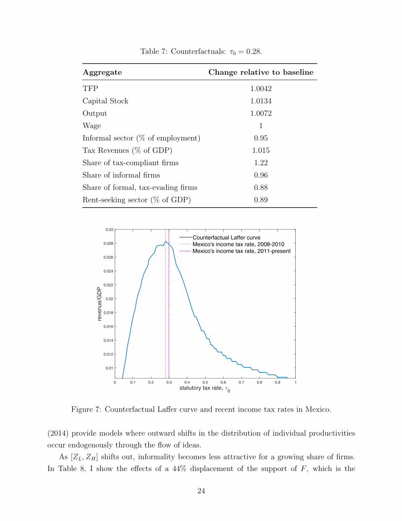
Table 7: Counterfactuals: τ0 = 0.28.

Aggregate Change relative to baseline

TFP 1.0042

Capital Stock 1.0134

Output 1.0072

Wage 1

Informal sector (% of employment) 0.95

Tax Revenues (% of GDP) 1.015

Share of tax-compliant firms 1.22

Share of informal firms 0.96

Share of formal, tax-evading firms 0.88

Rent-seeking sector (% of GDP) 0.89

statutory tax rate, τ0

0 0.1 0.2 0.3 0.4 0.5 0.6 0.7 0.8 0.9 1

reve

nue/

GD

P

0.01

0.012

0.014

0.016

0.018

0.02

0.022

0.024

0.026

0.028

0.03

Counterfactual Laffer curveMexico's income tax rate, 2008-2010Mexico's income tax rate, 2011-present

Figure 7: Counterfactual Laffer curve and recent income tax rates in Mexico.

(2014) provide models where outward shifts in the distribution of individual productivities

occur endogenously through the flow of ideas.

As [ZL, ZH ] shifts out, informality becomes less attractive for a growing share of firms.

In Table 8, I show the effects of a 44% displacement of the support of F , which is the

24

minimum increase that eliminates informality completely. The implied gains are very large,

with output increasing more than two times the baseline value.6 These calculations suggest

that if Mexico grew at a constant annual rate of 1.2 percent, which has been the average

over the past 25 years, it would take the country 70 years to grow out of informality.7

Tax revenues as a percentage of GDP increase, but less so than when we eliminate either

formal tax evasion or informality via full enforcement. This happens because, without any

changes in the enforcement parameters, the share of formal, tax-evading firms increase as

the economy develops. In fact, it turns out that the minimum growth necessary to eliminate

informality also coincides with the highest level of tax collection.

In Figure 8, I show the effects of economic development on revenues as a share of GDP,

the employment share of the informal sector, the share of formal, tax-evading firms, and tax-

evading expenditures as a share of GDP. The dotted vertical line indicates a growth factor

of 1.44—the minimum growth required to eliminate informality. Beyond that point, tax

revenues as a share of GDP steadily decline, the informal sector disappears, while both the

share of formal, tax-evading firms and tax-evading expenditures as a share of GDP continue

to increase. The latter partially explains the rise of professions such as accounting and law

as economies develop.

Table 8: Growth counterfactual—a 44% increase in [ZL, ZH ].

Aggregate Change relative to baseline

TFP 1.83

Capital Stock 2.4

Output 2.3

Wage 1.54

Informal sector (% of employment) 0

Tax Revenues (% of GDP) 1.53

Share of tax-compliant firms 3.48

Share of informal firms 0

Share of formal, tax-evading firms 3.52

Rent-seeking sector (% of GDP) 1.55

This growth counterfactual exercise provides a rationale for the existence of developed

countries with high tax evasion and/or avoidance. For instance, in 2009, per capita GDP

6Since population is constant, growth in output per capita is the same as growth in total output.7The growth rate is calculated using the World Bank’s World Development Indicators series for PPP-

adjusted GDP per capita at constant 2005 international dollars.

25

Growth factor0.5 1 1.5 2 2.5 3

reve

nue/

GD

P

0.01

0.015

0.02

0.025

0.03

0.035

0.04

0.045

0.05

Growth factor0.5 1 1.5 2 2.5 3E

mpl

oym

ent s

hare

of i

nfor

mal

sec

tor

0

0.1

0.2

0.3

0.4

0.5

0.6

Growth factor0.5 1 1.5 2 2.5 3

Sha

re o

f for

mal

tax-

evad

ing

firm

s

0

0.5

1

1.5

Growth factor0.5 1 1.5 2 2.5 3

Tax

-eva

ding

exp

endi

ture

s/G

DP

0.005

0.01

0.015

0.02

Figure 8: The effects of development tax revenues, informality, and formal tax evasion.

in Greece was 2.07 times that in Mexico. On the other hand, total income tax revenues as

a percentage of GDP were 6.9 for Greece, and 5.2 for Mexico, both falling well below the

OECD average of 11 percent.8

5 Concluding remarks

I presented a model where informal, formal tax-compliant, and formal tax-evading firms

coexist in equilibrium, as a result of the institutional environment. The theory predicts a

system of effective tax rates that relies on medium-sized firms to raise revenues. This result

links the evidence on the so-called “missing middle” in developing countries to a low capacity

to generate income tax revenues.

When the distribution of productivities improves over time, given taxes and enforcement

parameters, informality decreases, but formal tax evasion increases, thus limiting the state’s

8As before, per capita GDP data come from the World Bank’s World Development Indicators, whiledata on tax revenues come from the OECD’s Revenue Statistics. The OECD includes information on thecontribution of corporations to income tax revenues. However, these are not comparable with my calculationsfor Mexico, which include non-incorporated businesses.

26

capacity to raise tax revenues. If, as suggested by LaPorta and Shleifer (2014), lower infor-

mality is a byproduct of development, and not vice versa, then the tax authorities’ efforts

to raise revenues could be more effective when directed towards formal tax evasion.

In an attempt to keep the theory clear and tractable—but still suitable for quantitative

analysis—I have abstracted from some aspects of reality that would be interesting to consider

in future work. Specifically, there is evidence that the enforcement of some taxes increases

with firm size, as argued by Levy (2008). One could also think about how the rent seeking

interacts with sources of misallocation other than informality, such as financial constraints, as

in Lopez (2014). Last, the limited evidence on firm-level effective income tax rates suggests

that the returns to firm’s tax-evading efforts are not constant across firms. Allowing for

heterogeneity in both productivity and the returns to tax-evasion expenditures would bring

us a step closer to understanding the aggregate consequences of having an institutional

environment that rewards rent-seeking skills, and of firm-level political and bureaucratic

connections.

References

Acemoglu, Daron, 2005. “Politics and Economics in Weak and Strong States,” Journal

of Monetary Economics, 52, 1199-1226.

Allingham, M.G. and A. Sandmo, 1972. “Income Tax Evasion: A Theoretical Analy-

sis,” Journal of Public Economics, 1(3-4), 323-338.

Artavanis, Nikolaos, Adair Morse, and Margarita Tsoutsoura, 2015. “Tax

Evasion across Industries: Soft Credit Evidence from Greece,” NBER Working Paper No.

21552.

Axtell, R., 2001. “Zipf Distribution of US Firm Sizes,” Science, 293 (5536), 1818-1820.

Bergoeing, R., P. Kehoe, T. Kehoe, and R. Soto, 2002. “A Decade Lost and Found:

Mexico and Chile in the 1980s,” Review of Economic Dynamics, 5(1), 166205.

Bigio, Saki and Eduardo Zilberman, 2011. “Optimal Self-employment Income Tax

Enforcement,” Journal of Public Economics, 95, 1021-1035.

Cook, K. R. Huston, and T. Omer, 2008. “Earnings management through effective

tax rates: The effects of tax planning investment and the Sarbanes-Oxley Act of 2002,”

Contemporary Accounting Research, 25 (2), 447-471.

27

Fuentes Castro, Andres Zamudio Carrillo, and Sara Barajas, 2010. “Evasion

Global de Impuestos: Impuesto Sobre la Renta, Impuesto al Valor Agregado e Impuesto

Especial sobre Produccion y Servicio no Petrolero,” Centro de Estudios Estrategicos, Tec-

nologico de Monterrey.

Hsieh, Chang-Tai and Peter Klenow, 2014. “The Life Cycle of Plants in India and

Mexico,” Quarterly Journal of Economics, 129(3), 1035-1084.

Hsieh, Chang-Tai and Benjamin Olken, 2014. “The Missing ‘Missing Middle’,”Journal

of Economic Perspectives, 28(3), 89-98.

International Labor Organization, Statistical Update on Employment in the Infor-

mal Economy, June 2012.

Instituto Nacional de Estadıstica, Geografıa e Informatica, Censos Economicos,

2009, 2014.

Krueger, Anne, 1974. “The Political Economy of the Rent-Seeking Society,” American

Economic Review, 64(3), 291-303.

LaPorta, Rafael, and Andrei Shleifer, 2014. “Informality and Development,” Jour-

nal of Economic Perspectives, 28 (3), 109-126.

Leal-Ordonez, Julio C., 2014. “Tax Collection, the Informal Sector, and Productivity,”

Review of Economic Dynamics, 17, 262-286.

Lopez, Jose Joaquın, 2014. “Entrepreneurship and Rent Seeking under Credit Con-

straints,” Doctoral Dissertation, Department of Economics, University of Chicago.

Levy, Santiago, 2008. “Good Intentions, Bad Outcomes,” Washington, DC: Brookings

Institution.

Lucas, Robert E. Jr., 1978. “On the Size Distribution of Business Firms,” Bell Journal

of Economics, 9(2), 508-523.

Lucas, Robert E. Jr., 2009. “Ideas and Growth,” Economica, 76, 1-19.

Mayshar, Joram, 1991. “Taxation with Costly Administration,” Scandinavian Journal of

Economics, 93(1), 75-88.

28

McGuire, Sean T., Thomas C. Omer, and Dechun Wang, 2012. “Tax Avoidance:

Does Tax-Specific Industry Expertise Make a Difference?,” The Accounting Review, 87(3),

975-1003.

Mills, Lillian F., 1998. “Book-tax differences and internal revenue service adjustments,”

Journal of Accounting Research, 36, 343-356.

OECD, Revenue Statistics in Latin America and the Caribbean, 2015.

Perla, Jesse, and Christopher Tonetti, 2014. “Equilibrium Imitation and Growth,”

Journal of Political Economy, 22(1), 1-25.

Piketty, Thomas, Emmanuel Saez, and Stefanie Stantcheva , 2014. “Optimal

Taxation of Top Labor Incomes: A Tale of Three Elasticities,” American Economic Journal:

Economic Policy, 6(1), 230-71.

Restuccia, Diego, 2008. “The Latin American Development Problem,” Working Paper

318 , University of Toronto, Department of Economics.

SHCP, 2009. “Presupuesto de Gastos Fiscales 2009” Mexico, Secretarıa de Hacienda y

Credito Publico.

SHCP, 2010. “Distribucion del pago de impuestos y recepcion del gasto publico por deciles

de hogares y personas. Resultados para el ano 2010,” Mexico, Secretarıa de Hacienda y

Credito Publico.

Slemrod, Joel, 2001. “A General Model of the Behavioral Response to Taxation,” Inter-

national Tax and Public Finance, 8(2), 119–128.

Slemrod, Joel, 2007. “Cheating Ourselves: The Economics of Tax Evasion,” Journal of

Economic Perspectives, 21(1), 25–48.

Tullock, Gordon, 1992. “Economic Hierarchies, Organization and the Structure of Pro-

duction,” Cluver Academic Publisher, Boston, MA.

Ulyssea, Gabriel, 2014. “Firms, Informality and Development: Theory and evidence

from Brazil,” mimeo, Departamento de Economia, PUC-Rio.

Webber, Carolyn, and Aaron B. Wildavsky, 1986. “History of Taxation and Ex-

penditure in the Western World.” New York: Simon & Schuster.

29

The World Bank, 2015. World Development Indicators.

The World Bank, 2015. Enterprise Surveys.

Zilberman, Eduardo, 2015. “Audits or Distortions: The Optimal Scheme to Enforce

Self-Employment Income Taxes.” Journal of Public Economic Theory, forthcoming.

Appendix

Proof of Lemma 1. Suppose an agent has decided to be a formal entrepreneur. He will chose

to evade taxes as long as ΠE(Z) > ΠC(Z), and is indifferent between evading taxes and

complying whenever ΠE(Z) = ΠC(Z). The indifference condition is given by

ZEΨ(w, r)− 1

φ[1 + log (τ0φZEΨ(w, r))] = (1− τ0)ZEΨ(w, r),

which simplifies to

τ0Ψ(w, r)ZE =1 + log(τ0φΨ(w, r)ZE)

φ. (16)

Notice that the left hand side of (16) is the cost of being compliant, while the right hand

side represents the cost of evading taxes. Let X = τ0φΨ(w, r)Z. The expression above can

then be rewritten as X = 1 + log(X), which has a unique fixed point at X∗ = 1. Moreover,

this fixed point is also a tangency point, with X > 1 + log(X) whenever X > 1. This

condition pins down the productivity cutoff for tax evasion at ZE = [τ0φΨ(w, r)]−1. For

Z > ZE, the cost of being compliant exceeds the cost of tax evasion. For Z < ZE, B(Z) < 0,

which violates the non-negativity constraint, while B(ZE) = 0. Therefore, entrepreneurs

with ability Z ≤ ZE will choose B(Z) = 0, and pay the statutory tax rate, while those with

ability Z > ZE will pay B(Z) > 0 in order to evade taxes. This concludes the proof.

Proof of Lemma 2. Assume there is a ZP > 0 such that ω(ZP ) > (1− τ0).Case I: ZI < ZE. I start with the case in which there are some formal firms that chose

to comply. In this case, the indifference condition is given by ΠI(ZI) = ΠC(ZI), or

ω(ZI)ZIΨ(w, r) = (1− τ0)ZIΨ(w, r),

which simplifies to

ω(ZI) = (1− τ0)

30

The function ω(Z) ∈ [0, 1] is decreasing, and strictly decreasing in (0, 1).9 Since there is

a ZP > 0 such that ω(ZP ) > (1− τ0), by the Intermediate Value Theorem, there exists a

unique ZI such that ω(ZI) = (1− τ0).

Case II: ZI > ZE. In this case only informal and tax-evading firms exist. First notice

that we can write the profits of informal firms that are bound by the detection threshold as

ΠI(Z) = (1− (1− α)θ)

[(1− α)θ

w

] (1−α)θ1−(1−α)θ

Dαθ

1−(1−α)θZ1−θ

1−(1−α)θ − rD

Since there are no formal tax-complaint firms, it has to be that ΠI(ZE) > ΠE(ZE). As

Z increases and the detection threshold binds, the profit function ΠI(Z) will be strictly

increasing and strictly concave. Since ΠE(Z) is strictly increasing and stricly convex for

Z > ZE, it crosses ΠI(Z) only once, at ZI . This concludes the proof.

Proof of Lemma 3. The profit function Π∗(Z;w, φ, τ0, D) is strictly increasing in Z with

Π∗(0;w, φ, τ0, D) = 0, so for any w > 0 there is a unique ZW > 0 such that Π∗(ZW ;w, φ, τ0, D) =

w. Clearly, V (Z) = Π∗(Z;w, φ, τ0, D) for any Z ≥ ZW and V (Z) = w otherwise.

9As Z increases, the size constrain binds and µ(Z) increases, so ω(Z) decreases.

31