Copyright © 2013, 2014 by Shawn Cole, Xavier Giné, and James Vickery

Working papers are in draft form. This working paper is distributed for purposes of comment and discussion only. It may not be reproduced without permission of the copyright holder. Copies of working papers are available from the author.

How Does Risk Management Influence Production Decisions? Evidence from a Field Experiment Shawn Cole Xavier Giné James Vickery

Working Paper

13-080 September 9, 2014

How Does Risk Management Influence Production Decisions?

Evidence from a Field Experiment*

Shawn Cole (Harvard Business School and NBER) Xavier Giné (World Bank)

James Vickery (Federal Reserve Bank of New York)

First Version: February 2011 This version: September 2014

Weather is a key source of income risk, particularly in emerging market economies. This paper uses a randomized controlled trial involving a sample of Indian farmers to study how an innovative rainfall insurance product affects production decisions. We find that insurance provision induces farmers to shift production towards higher-return but higher-risk cash crops, particularly among educated farmers. Our results support the view that financial innovation can mitigate the real effects of uninsured production risk. Addressing the puzzle of low adoption, we show payouts improve trust in the product, and that farmers shield payouts from claims by relatives.

* Email: scole@hbs.edu, xgine@worldbank.org and james.vickery@ny.frb.org. We owe a particular debt to K.P.C. Rao for his efforts in managing the field work associated with this study, and to his survey team. Outstanding research assistance was also provided by Fenella Carpena, Kevin Connolly, Lev Menand, Veronica Postal, Jordi de la Torre, and Wentao Xiong. We also thank many seminar and conference participants and several discussants for their ideas and suggestions. Financial support for this project was provided by the Research Committee of the World Bank and the Division of Research and Faculty Development at Harvard Business School. Views expressed in this paper are those of the authors, and do not necessarily reflect the opinions of the World Bank, the Federal Reserve Bank of New York or the Federal Reserve System.

1

1. Introduction

Small entrepreneurial firms around the world are exposed to a wide range of income risks,

including recessions, demand shifts, technology shocks, weather, and natural disasters.

Reflecting these risks, around one-third of US business establishments fail within two years

(Puri and Zarutskie, 2012). Risks associated with entrepreneurship may be even greater in

volatile emerging market economies. For a risk-averse individual, these uninsured risks can

be a significant disincentive to engage in entrepreneurial activity (Moskowitz and Vissing-

Jorgensen, 2002; Banerjee and Newman, 1993).

This paper studies a financial innovation designed to mitigate income risk among

small Indian agricultural producers. Our sample of farmers is located in a semi-arid region in

which variation in monsoon rainfall is the dominant source of production and income risk. In

this context, we study the effects on behavior of a rainfall index insurance policy, which

partially insures against a poor monsoon by providing a payout contingent on low measured

local rainfall.

Our goal is to estimate the effects of the rainfall insurance on real production and

investment decisions by farmers. Given that the decision to purchase insurance is typically

endogenous, we use a randomized controlled trial (RCT) approach to elicit the causal effect

of insurance coverage on behavior. At the start of the monsoon, a randomly selected subset

of farmers (the “treatment group”) is provided with 10 rainfall insurance policies with a

combined market value of approximately 1,000 Indian rupees (equivalent to ca. $20 US at

the time of our study). This represents a significant amount of coverage for our sample; the

maximum insurance payout of 10,000 rupees (Rs.) is equivalent to about 90% of median

household savings. We then study how this insurance provision influences subsequent

production decisions such as crop choice and usage of agricultural inputs, compared to a

control group promised a fixed payment equal to the estimated actuarial value of the

insurance.

We find that, while insurance provision has little effect on total agricultural

investments, it significantly shifts the composition of investments towards riskier production

activities. In particular, treated households increase production of the main cash crops grown

2

in our study areas, castor and groundnut. These crops produce higher expected returns, but

are also more sensitive to deficient rainfall. We find that insured farmers are more likely to

plant these two cash crops, sow more land with them and devote a larger amount of

agricultural inputs to them relative to uninsured farmers. Quantitatively, the fraction of

farmers planting cash crops is 6 percentage points higher for the treatment group (p=0.041),

a 12 percent increase relative to the control group, about half of whom plant cash crops in the

year of our study. The evidence suggests the impact of insurance is primarily on the

extensive margin: it has large effects on the decision to sow cash crops, but little effect

among the subset of farmers with the highest cash crop investments.

We then test whether the treatment effect varies by household characteristics. We find

that the effects of insurance on behavior are concentrated among educated farmers, measured

either by years of schooling or an indicator variable for whether the farmer is literate. Among

literate farmers, assignment to the insurance treatment group increases the likelihood of

investing in cash crops by 15 percentage points; in contrast, for illiterate farmers, the

treatment effect is close to zero. This result is consistent with the view that new financial

products predominantly assist more-advantaged households with low costs of accessing the

financial system or higher financial literacy.

Using data on the timing of agricultural decisions, we find that the effects of

insurance provision on production decisions occur ex ante, prior to the end of the insurance

coverage period, when the insurance payout and monsoon rainfall are still uncertain. We also

conducted a second follow-up survey in the following year, after insurance payouts were

disbursed, to study how insurance payouts were ultimately spent by farmers. While the

statistical power of this analysis is relatively low, our results suggest that payouts were

mainly saved for the next monsoon or used to pay down expensive sources of credit.

A. Related literature

Although insurance is a key function of the global financial system, we have only a partial

understanding of how insurance provision causally influences real economic behavior and

risk-taking. This study is among the first in a small body of recent research which uses an

RCT approach to study the causal relationship between insurance and agricultural decisions.

3

Karlan et al. (forthcoming) randomly allocate cash grants and discounted insurance offered

by an NGO, or both, to farmers in Ghana, finding that cash grants do not affect investment,

but that insurance does. Mobarak and Rosenzweig (2012) conduct a randomized evaluation

which uses subsidies to induce households to purchase insurance against late monsoon

arrival: while their main interest is the interaction between insurance demand and informal

risk-sharing, they also find evidence that insured households plant riskier varieties of rice,

although planting may happen after knowledge of the payout. In a related study, Cai et al.

(forthcoming) finds evidence from China that hog insurance increases investment in hogs.1

Several features distinguish our paper from this complementary literature. First, our

design allows us to study how insurance affects the timing of decisions, and to distinguish

clearly between ex ante effects of insurance (effects on behavior during the insurance

coverage period), and ex post effects due to the receipt of insurance payouts or the

anticipation of future payouts. Second, we study a relatively mature, commercially available

insurance policy, one that many farmers have purchased at least once over the previous five

years. It is less likely in this setting that changes in behavior are due to the novelty of the

product. Third, we find large differences in the treatment effect of insurance by educational

attainment, although not along other household characteristics. Finally, we present the first

(and to our knowledge, only) systematic evidence on how insurance payouts are used. Taken

together, the nascent literature demonstrates in a variety of institutional and economic

settings that access to insurance leads to an increase in risky production activities.

Our analysis is relevant to the vast literature on risk, growth, and technology adoption

in emerging market economies (e.g., Acemoglu and Zilibotti, 1997; King and Levine, 1993;

Banerjee and Newman, 1993; Rosenzweig and Binswanger, 1993). While technological

improvements from the “Green Revolution” such as high-yield crops and chemical fertilizer

has dramatically increased global agricultural productivity, traditional practices still prevail

in many areas (Duflo, Kremer and Robinson, 2008; Hazell, 2009; Foster and Rosenzweig,

2010). Our evidence suggests that limited insurance against production risk is one reason

1 Emerick et al. (2014) study the introduction of a drought-resistant rice variety that both reduces the yield

variability induced by weather and increases average yields. They also find that the rice variety leads to increases in

land cultivated, investment in fertilizer and the use of a more labor intensive planting method.

4

why firms limit investments that produce high expected returns but involve risk.

Correspondingly, financial innovation that “completes” missing markets, like the insurance

policy we study, may boost risk-taking and technology adoption. This channel may account

for part of the link between finance and growth identified in prior research (Levine, 2005;

Beck, Levine and Loayza, 2000).2

A related literature explores the link between finance and entrepreneurial activity in

developed economies, although research to date generally focuses on credit constraints (e.g.,

Black and Strahan, 2002; Hurst and Lusardi, 2004). Most closely related, Fan and White

(2003) find evidence of greater business ownership associated with the option to declare

bankruptcy, a procedure that allows entrepreneurs to shield future income and some assets

from creditors, limiting the downside risk of entrepreneurial activity. Insurance and

investment risk tolerance has also been studied in the context of large, sophisticated

corporations (e.g., Campello et al., 2011; Pérez-Gonzáles and Yun, 2013).

Finally, recent household finance research has emphasized two major pitfalls that

prevent customers from taking full advantage of financial innovations: predatory behavior

and mistakes due to low financial literacy (Agarwal et al., 2009, Campbell, 2006). Our

finding that changes in behavior are concentrated among educated farmers may be indicative

of a lack of trust in the product, or understanding of it, among less-educated farmers.

2. Background and experimental design

Consumption risk-sharing, though surprisingly effective in mitigating nonsystematic income

shocks (Cochrane, 1991; Townsend, 1994), has been found to be incomplete, particularly for

spatially correlated shocks such as weather. Droughts, for example, have significant negative

effects on economic well-being and health for rural households in India and other emerging

market economies, suggesting that the risk of drought is underinsured (e.g. Burgess et al.,

2 Our analysis is also related to research studying the effects of climate change on agricultural productivity. Guiteras

(2009) estimates that predicted climate change from 2010-2039 will reduce crop yields by 4.5-9 percent. While

rainfall insurance cannot of course affect the climate, it may enable farmers to continue producing risky crops in the

face of greater climate variability, mitigating the real impact of climate change.

5

2013; Maccini and Yang, 2009; Jayachandran, 2006; Rose, 1999; see Cole et al., 2013, for

further references).

When it is not possible to insure consumption against income risks such as drought,

individuals may reduce uninsured income risk by smoothing their income ex ante, selecting

production and investment activities that generate a less volatile income stream at the cost of

lower average income (Morduch, 1995; Gollier and Pratt, 1996; Walker and Ryan, 1990).

Corporate finance research makes an analogous prediction for firms: in the presence of

financial constraints, a firm facing nondiversifiable risks will invest less in additional risky

projects, particularly when the project return is positively correlated with the prior existing

risk exposure (Froot and Stein, 1998).

Income smoothing tactics for farmers include intercropping by drought tolerance,

spatial separation of plots, shifts in the timing and staggering of planting, moisture

conservation measures such as bunds, furrows and irrigation, and income diversification

between agricultural and non-agricultural sources. Several papers find suggestive evidence of

costly income smoothing by agricultural firms in developing countries (e.g., Rosenzweig and

Stark, 1989; Morduch, 1995; Dercon, 1998; Dercon and Christiaensen, 2011).3

The key hypothesis tested in this paper is that the provision of insurance against

rainfall risk will induce households to allocate more resources to higher-risk, higher-yield

investment and production activities. To fix ideas, we illustrate this hypothesis using a

simple theoretical model of insurance and production in which households choose between

two production methods: one safe, the other higher-yielding but risky (Appendix A).

Insurance against production risk induces risk-averse farmers to allocate more resources to

the high-yield production method. While our model uses a simple CARA-normal setup that

yields a closed-form solution, this basic prediction will apply to nearly any model with risk-

averse agents, incomplete markets and production risk.

3 Rosenzweig and Stark find that farmers with more volatile profits are more likely to have a household member

engaged in steady wage employment. Morduch suggests that households close to a subsistence level of consumption

devote a larger share of land to safer crop varieties. Dercon finds Tanzanian farmers with a large stock of liquid

assets engage in higher risk agricultural activities. Dercon and Christiaensen find that fertilizer purchases are lower

among poorer Ethiopian households, in part due to their lesser ability to smooth adverse shocks ex post. Rosenzweig

and Binswanger (1993) estimate that a one standard deviation increase in the variability of monsoon onset would,

through reduced risk-taking, reduce agricultural profits by 15 percent for the median household.

6

We test the above theoretical prediction in a setting where firms face a dominant,

exogenous source of production risk: variation in local monsoon rainfall. Rainfall is cited as

the most important source of risk by 89% of farmers in our study areas. Although these local

rainfall shocks are approximately uncorrelated with aggregate asset returns, farmers in our

sample have a large, non-diversified exposure to local weather risk. Recognizing the

importance of rainfall risk, Indian insurers have recently developed innovative retail index

insurance products designed to pay out when realized monsoon rainfall is poor. We study a

particular policy developed by the private Indian insurer ICICI Lombard. Our analysis builds

on a series of experiments and surveys that we have conducted since 2004 in Andhra

Pradesh, India (Cole et al., 2013; Giné, Townsend and Vickery, 2008). This previous work

has focused on studying the determinants of rainfall insurance demand, rather than the

impact of insurance on behavior.4

A. Crop choice and risk-taking

The model in Appendix A considers the tradeoff between high-risk, high-yield and low-risk,

low-yield production activities. The analog in our empirical analysis is the allocation of

agricultural inputs across crop types. During the main cropping season (June to November)

in our study areas, farmers grow a variety of cash and subsistence crops that vary by

sensitivity to low rainfall. The primary cash crops grown in the study areas are castor and

groundnut, two rain-fed oilseeds, as well as paddy, which is almost exclusively irrigated and

thus less subject to rainfall risk (84% of paddy plots in our empirical sample are irrigated).

The main subsistence crops grown in the area are sorghum and legumes (red gram, Pigeon

pea and to a lesser extent green gram).

Cultivation costs for the main cash crops exceed those of subsistence crops and range

between Rs. 5,000 and Rs. 9,000 per hectare ($94 to $168 US), if the recommended amounts

of organic and inorganic fertilizer are applied.5 Based on the local District Handbook of

4 Although some of our earlier research also adopts a field experimental approach (Giné and Yang, 2009 and Cole et

al. 2013), uptake has been too limited to allow an assessment of the impact of insurance on real decisions. Two

related laboratory experiments conducted by Lybbert et al. (2010) and Hill and Viceisza (2012) suggest that, over

time, subjects learn about insurance and change behavior accordingly. 5 Input recommendations (used to calculate 2009 production costs per hectare for castor, groundnut, sorghum, and

red and green grams) come from the University of Agricultural Sciences in Bangalore (UAS, 1999).

7

Statistics, average yields for castor are 600 Kg per hectare if fertilizer is used, which would

generate Rs. 10,896 in revenue at 2009 prices. Groundnut yields are 540 Kg per hectare with

fertilizer, corresponding to Rs. 11,702. Sorghum yields with fertilizer are 700 Kg per hectare

or Rs. 4,788 and red gram yields are 300 Kg or Rs. 5,791. Thus, expected profits for castor

and groundnut are indeed higher at Rs. 2,771 and Rs. 2,951 compared to sorghum (negative

Rs. 212) and red gram (Rs. 141).

In terms of water requirements, researchers at the Central Research Institute for

Dryland Agriculture (CRIDA) estimate that castor grown in Mahbubnagar under rain-fed

conditions requires 625 mm of accumulated rainfall over the season if sown around the

normal planting date while groundnut in Anantapur requires 533 mm. Red gram requires a

similar amount of accumulated rainfall, 523 mm, but in contrast, sorghum only requires 376

mm and green gram 278 mm.6

To summarize, castor and groundnut are more profitable on average than other crops

grown in our study areas, but have higher water requirements and therefore are more

sensitive to drought.

B. Product description

The rainfall insurance policies offered in this study are an example of “index insurance,” that

is, a contract whose payouts are linked to a publicly observable index like rainfall,

temperature or a commodity price. Unlike traditional insurance products, index insurance is

not generally subject to moral hazard or adverse selection problems, because payouts are

linked to an exogenous, publicly observable variable, in this case, rainfall measured at a local

rain gauge. Index insurance also involves lower administrative costs because no claims

verification process is required. However, rainfall insurance only covers rainfall-related

losses and may entail significant basis risk, especially if the household is located too far from

the relevant weather reference station.7

6 Based on personal communication from Dr. Bodapati Rao and Dr. Vijay Kumar, Principal Scientists at CRIDA.

7 In our study, villages are generally located within 10km of the reference weather station. Given the relatively flat

terrain one may think that basis risk is likely to be relatively low, at least for our sample. However, Section 5 reports

evidence consistent with basis risk.

8

Information frictions and high transaction costs have limited the commercial success

of agricultural insurance. Insurance companies have initiated a number of index insurance

pilots in recent years in the hope of developing a financially sustainable product that farmers

will buy (World Bank, 2005; Skees, 2008). Today, rainfall insurance is one of the core

product offerings of Indian agricultural insurance providers with over 10 million farmers

covered by index policies. Clarke et al. (2012) and Giné et al. (2012) provide non-technical

overviews of this market and further institutional details.

The policies we study are designed and underwritten by ICICI Lombard, a large

Indian insurance firm. Payoffs are calculated based on measured rainfall at a nearby

government rainfall station or an automated rain gauge operated by a private third-party

vendor. ICICI Lombard policies divide the monsoon season into three contiguous phases of

35-45 days each, corresponding to sowing, flowering, and harvest. The study offered only

Phase I policies, which cover the first and most critical period of the season.

Each insurance contract specifies a threshold amount of rainfall, designed to

approximate the minimum required for successful crop growth. The start date of the policy is

defined as the first date at which cumulative rainfall since June 1 is at least 50 mm (or

defaults to July 1 if June rainfall is below 50mm). Payouts are then determined based on

cumulative rainfall during the 35 days following the start date. The policy pays out if

cumulative rainfall during this coverage period is below a threshold known as the “strike.”

Payouts are linear in the rainfall deficit relative to the exit, or are equal to a fixed maximum

amount of Rs. 1000 per policy if rainfall is below a second, lower threshold call the “exit.”

Since payouts are linked to rainfall levels determined by a nearby gauge, treated

farmers received policies linked to one of five weather stations, depending on their village.

Because the 2009 monsoon turned out to be significantly below average, three of these five

policies provided positive payouts ex post, with one policy paying out the maximum payout

of Rs. 1,000 per policy, corresponding to a total payout of Rs. 10,000 for each treated farmer.

9

C. The insurance experiment

Our sample consists of 1,479 farmers drawn from 45 villages in one drought-prone district of

Telangana (Mahbubnagar) and another in Andhra Pradesh (Anantapur).8 Two-thirds of the

sample participated in previous research we conducted on rainfall insurance; these were

originally selected via a stratified random sample of land-owning farmers in 37 study

villages in 2004 (see Giné et al., 2008, for details). To improve statistical power for this

study, an additional 500 households were drawn from these 37 villages as well as 8 nearby

villages.

Figure 1 presents the timeline of events. Each farmer received a home visit from a

member of a trained team of enumerators from the agricultural research organization

ICRISAT between June 4 and July 13, 2009, coinciding with the onset of the 2009 monsoon

season.9 During the visit, the enumerator first conducted a short baseline survey, collecting

demographic information and data on practices by the farmer during the previous monsoon.

They then explained the recommended fertilizer dosages for castor and groundnut, the two

main rain-fed cash crops in the area, as well as the concept of insurance, and gave specific

details about the policies offered by ICICI Lombard.

[Insert Figure 1 here]

The farmer then received a scratch card (similar to the format of a scratch-off lottery

ticket sold in the United States), revealing treatment assignment. The key treatment for the

purposes of this paper is the assignment of the household to either an insurance group or a

control group. Farmers in the insurance treatment group received a certificate for 10 Phase-I

weather insurance policies, similar to those sold in the region in previous years. “Control”

farmers received a post-dated check of Rs. 200 (our estimate of the expected payouts of these

8 At the time of the study, the newly formed state of Telangana was still part of Andhra Pradesh.

9 Although the distribution of all insurance policies was planned to be completed prior to the occur before the start

of the insurance coverage period, delays in the shipping of policy certificates from ICICI headquarters in Mumbai

resulted in a significant minority (40 percent) of the initial visits occurring on or after the policy activation date. In

these cases, however, distribution occurred close to the start of the activation period, within five days on average.

For the sample as a whole, only six percent of farmers had started to plant by the time the initial household visit and

insurance assignment occurred. The small amount of prior monsoon investments occurred prior to the distribution of

insurance may if anything mean that our results are slightly attenuated relative to the case where insurance policies

were distributed earlier (since earlier distribution would have given farmers more time to adjust behavior in in

response to the knowledge of insurance coverage).

10

10 policies) that could be cashed at the local BASIX branch. This compensation was offered

to ensure that differences in behavior between the insurance and control group would be due

to the state-contingent nature of the insurance, rather than any wealth effects arising from the

expected value of the insurance. The date when the check could be cashed coincided with the

expected timing of insurance payouts.

A second independent treatment also provided via the scratch card, involved coupons

for discounts on locally appropriate inorganic fertilizer (DAP in Anantapur, NP fertilizer in

Mahbubnagar). Unfortunately the implementation of this treatment was largely unsuccessful

because the incentives were too small.10 For that reason, we do not study it here, although our

analysis controls for the household’s fertilizer discount treatment status in our analysis.11

Treatments were assigned randomly and independently across households. The use of

scratch cards ensured that neither the respondent nor the enumerator had prior information

about the household’s treatment status. Farmers also had the option to purchase additional

insurance policies from the local vendor, BASIX, although few did so in practice.

In October and November 2009, after the growing season, the ICRISAT team

revisited each household, and conducted the first of two follow-up surveys. In addition to

demographic data, the survey collected information on livestock, financial assets (including

savings, loans, and insurance), agricultural investments and production decisions during the

monsoon, as well as attitudes towards and expectations of weather and insurance payout, and

risk-coping behavior. Although payouts had not been made by the time of the first follow-up

survey, because of the poor monsoon in 2009, 93% of the farmers in the treated group

expected to receive a payout. Roughly the same percentage expected final crop yields to be

below average.

Payouts to the insurance and control group were made in December 2009 and January

2010. This timing is well after one might have expected, given that policies indicate a

10

The number of coupons (or bags) with a subsidy was calibrated to fertilizer usage reported in a survey conducted

in 2006. According to that survey, 70 percent of farmers in Mahbubnagar but only 34.4 percent in Anantapur had

used fertilizer and those that did would purchase at most two bags. However, follow-up data collected in November

2009 revealed much higher fertilizer usage (see Section 4.F for details). 11

Our results are almost identical whether or not we control for fertilizer treatment status; this is unsurprising given

that the fertilizer treatment is statistically independent of our main insurance treatment, by design.

11

settlement date of “thirty days after the data release by data provider and verified by Insurer.”

However, the timing was relatively consistent with previous years. The long timeframe

reflected both slow release of rainfall data and slow processing by ICICI Lombard.

Between April and July 2010 the team of enumerators revisited all farmers to conduct

the second follow-up survey.12 The goal of this final round of data collection was to measure

how payouts were used. The survey collected more detailed information on landholdings,

livestock, financial assets, agricultural investments and production decisions during the Rabi

(winter season), household consumption as well as attitudes towards the insurance product,

the use of payout funds (if any), transfers to and from other households and other risk-coping

behavior. Although our main focus is to measure the ex ante effects of insurance on behavior

before the resolution of uncertainty and receipt of payouts, we study these ex post effects of

insurance in Section 5.

Figure 2 plots total cumulative rainfall (blue line) and cumulative “index” rainfall

(measured from the policy start date), for each of the five policies. The gold horizontal lines

represent the strike (top) and exit (bottom) levels of rainfall for the rainfall station. For

example, in Naryanpet, rainfall was very low in June, never reaching the trigger amount of

50 mm. Thus, the policy started automatically on July 1. Cumulative rainfall then quickly

crossed the exit (5mm) level, but only reached 16 mm during the coverage period, well

below the strike of 50mm. Each policy therefore triggered a payout of Rs. 10 x (50-16), or

Rs. 340, or Rs. 3,400 per treated farmer, since each treated farmer received ten policies.

Farmers in Anantapur received per-policy payouts of (30-10) x 10 = Rs. 200 (i.e. Rs. 2,000

in total). In Hindupur, no rainfall fell in the month of July, triggering the ‘exit’;

consequently, farmers received a payout of Rs. 1,000 per policy, or Rs. 10,000 in total. As

we describe below, many of these payouts were quite large (Rs. 10,000 is approximately

$200, an amount 50% greater than the average household's financial assets).

[Insert Figure 2 here]

12

There is a small amount of attrition between the first and second follow-up surveys -- out of 1,479 farmers that

completed the first two surveys, only 1,459 completed the second follow-up survey.

12

3. Summary Statistics

Table 1 presents baseline summary statistics about household characteristics, savings, credit,

insurance knowledge and other variables. These statistics are drawn from the initial baseline

survey whenever possible. Since logistical constraints limited the length of the initial

baseline survey, however, a subset of the variables were collected using recall questions in

the first follow up survey conducted just after the monsoon. Respondents in the follow up

survey were asked to report information about fixed characteristics (e.g., years of schooling)

and to provide recall data on the value of livestock and other assets as of June 2009.

[Insert Table 1 here]

Panel A presents demographic data. The average household has 5.35 members with a

50-year old household head. Household heads are usually (91%) male, and on average have

obtained 3.75 years of schooling, with over half (54%) self-reporting being “unschooled.”

Literacy is low, with only 44 percent and 41 percent of heads self-reporting being able to

read and write, respectively. These statistics are similar to those reported in our previous

work (e.g., see statistics in Cole et al. 2013, which are based on a 2006 survey instrument).

Given that insurance provision was randomized, we should not observe systematic

differences in characteristics between the treatment and control groups. This hypothesis is

tested in Online Appendix Table OA1, for demographic characteristics (Panel A), financial

assets and credit (Panel B), livestock and other assets including land (Panel C), and

agricultural investments during the previous monsoon in 2008 (Panel D). Validating the

randomization, we find a statistically significant difference between the two groups for only

one out of 53 variables (the use of non-traditional savings). Furthermore, an F-test of the null

hypothesis that all average characteristics are the same for the treatment and control groups

cannot be rejected (P-value = 0.79).

Table 2 presents summary statistics for agricultural investment decisions during the

2009 monsoon, based on the first follow up survey conducted in late 2009. We collected

information on planting decisions and usage of different agricultural inputs, including seeds,

13

fertilizer, manure, pesticide, irrigation and hired labor. For five inputs, we also separately

measure the value of the input used only for the production of castor and for groundnut, as

well as the area of land sown under castor and groundnut.

A very high share (93%) of farmers planted some crop, and roughly half (48%)

planted cash crops (castor or groundnut). Fewer farmers planted cash crops in 2009 than

2008, reflecting the poor 2009 monsoon. Also reflecting the poor monsoon, 18% of farmers

abandoned their crop during the 2009 monsoon season.

[Insert Table 2 here]

Table 3 summarizes contract details and realized payouts for the five insurance

policies (recall that farmers were given policies linked to different rainfall stations depending

on the location of the farmer’s village). Three of the five insurance contracts realized a

positive payout, and the 242 treated farmers with insurance indexed to Hindpur station

rainfall received the maximum payout of Rs. 1,000 per policy (Rs. 10,000 in total). We use

variation in payouts across rainfall stations to distinguish between ex ante and ex post effects

of insurance provision (see section 4), and to track how insurance payouts were ultimately

used by farmers (see section 5).

[Insert Table 3 here]

4. Estimation results

A. Baseline estimates

Table 4 presents the estimated average treatment effects of insurance provision on farmers’

agricultural decisions, based on the investment variables summarized in Table 2. We analyze

four outcome variables: (i) a dummy equal to one if any agricultural inputs were used during

the monsoon, (ii) the area of land sown, (iii) the market value of agricultural inputs used, and

(iv) the value of agricultural inputs purchased. For the first three outcome variables, we

14

separately study inputs used for the production of castor and groundnut.13 These cash crop

estimates are presented separately in the table.

[Insert Table 4 here]

In Panel A, each outcome variable is regressed on a dummy for whether the

household received the insurance treatment (the key variable of interest), a set of village

dummies, and a dummy for each fertilizer treatment. A tobit estimator is used when the

dependent variable is continuous, while a probit is used for the “any inputs used” dummy. To

conserve space, only results for the key coefficient on the insurance treatment dummy are

presented.

Studying total investments (the first column of results), we find a positive, although

statistically insignificant, effect of the insurance treatment on the quantity of inputs used or

the area of land cultivated. However, when the analysis is restricted to castor and groundnut

investments, the treatment effects become much larger, and are also statistically significant at

the 5% level or lower in each specification. Quantitatively, assignment to the insurance

treatment group increases the probability of planting cash crops by 6 percentage points (or 12

percent). Ln(1+land planted for cash crops) increases by 0.163, equivalent to a 27 percent

increase in land sown for a farmer who would have planted 2 acres of cash crops in the

absence of the treatment.14

To summarize, we find significant substitution effects towards cash crop investments,

although no significant effect on total agricultural expenditures. This latter result could be

consistent with the presence of fixed short-run production factors (e.g. a given amount of

land, which cannot be easily adjusted in the short run), or the presence of financial

constraints. It may also simply reflect our limited statistical power.

Specifications in Panel B of Table 4 are otherwise identical, but include measures of

household socioeconomic status as additional controls, as a robustness check. Adding the

13

We did not collect this information for the “market value of inputs purchased” variable. 14

If the farmer originally planned to sow two acres of cash crops, our point estimate implies that the new quantity of

land planted for cash crops will be exp((ln(1+2)+0.163)-1) = 2.53 acres, a 26.5% increase. Recall that about half the

farmers in our sample plant no cash crops during the 2009 monsoon. A small minority planted no crops at all. This is

due to the poor realized quality of the 2009 monsoon.

15

controls has little effect on our estimates, consistent with the random assignment of farmers

to the treatment and control groups. Table OA2 of the Online Appendix also reports

regression results for cash crop expenditures split up by input type (seeds, fertilizer, etc.).

Table 4 reports average treatment effects – Figure 3 instead plots the cumulative

distribution function of investment in cash crops by insurance treatment status. This plot

suggests that the effect of the insurance treatment is quite non-linear. Insurance causes a

sizeable number of farmers to switch on the extensive margin from not growing cash crops

into growing cash crops, consistent with the probit regression estimates. But for farmers in

the top part of the distribution of cash crop investments, insurance provision has little or no

effect on cash crop inputs used. In other words, the effect of insurance is primarily on the

extensive rather than the intensive margin.

[Insert Figure 3 here]

Figure 3 also illustrates that there is a discrete jump in the level of cash crop

investment once the farmer decides to invest a positive amount. This points to the presence

of scale economies; farmers do not sow a given crop below a minimum scale. Around this

decision threshold, the provision of insurance against income risk makes farmers more

willing to invest a positive amount in castor and/or groundnut. According to our data, the

minimum area cultivated under cash crops is 0.5 acres, accounting for 10 percent of average

landholdings. For farmers planting cash crops, the median area under cash crops cultivation

is 3 acres (70 percent of landholdings).

B. Heterogeneous treatment effects

In Table 5, we test for heterogeneity in the treatment effect by measures of household wealth,

education and expectations. We estimate regressions of the form:

outcome = f(a + b. insurance + c. characteristic + d. insurance x characteristic + … + e)

where “insurance” is the dummy for insurance treatment status, and “characteristic” is the

source of heterogeneity of interest (e.g. wealth, education etc.). Our primary interest is the

coefficient d on the interaction term. As in Table 4, we consider three outcome variables, a

16

dummy for whether the farmer plants cash crops, the value of their investment in cash crops,

and the area of land planted with cash crops.

[Insert Table 5 here]

We first study how the insurance treatment effect varies with two wealth measures:

acres of land owned, and a wealth index derived as the first principal component of asset

holdings (see Appendix B for details of how this variable and selected other variables used in

this study are constructed). These wealth variables are included as interaction characteristics

one at a time. It is unclear theoretically what effect is expected; on one hand, wealthier

households may have better ex post consumption insurance (as in Mobarak and Rosenzweig,

2012), making them less likely to respond to rainfall insurance. On the other hand, wealthy

farmers may be able to more easily adjust agricultural practices in response to a shift in the

risk-return frontier introduced by insurance (e.g., because they are less financially

constrained). Empirically we find mixed and weak results – the treatment effect is increasing

in landholdings but decreasing in the wealth index; neither relationship is statistically

significant. The direct effect of wealth using either variable is highly positive and statistically

significant, as expected; that is, wealthy farmers are much more likely to invest in cash crops.

Next, we consider heterogeneity by two measures of educational attainment: log years

of education, and a dummy for whether the household head is literate. Strikingly, we find

large, positive, statistically significant interaction effects for both measures, implying that the

treatment effect of insurance provision on production behavior is concentrated amongst

educated households. This heterogeneity by educational attainment is economically

important as well as statistically significant. For literate farmers, assignment to the insurance

treatment group increases the likelihood of investing in cash crops by 15 percentage points;

for illiterate farmers, the treatment effect is close to zero and statistically insignificant.

Next, we use ex post realized payouts as the interaction variable. This provides a test

of whether farmers’ investment responses might reflect their expectation of receiving a high

payout in the future (e.g. because of early information that the monsoon is likely to be poor).

This interaction variable is quantitatively small and statistically insignificant, implying that

the investment response is not driven by this anticipation effect.

17

Finally, we consider two specific measures of the farmer’s knowledge of insurance

(measured at baseline) as the interaction variables. Neither of these variables is statistically

significant. Interestingly, it appears to be the farmer’s overall education level, not their

specific knowledge of the insurance policy at baseline, that matters for the strength of the

treatment effect. A possible interpretation of this finding is that a well-educated farmer, even

if unfamiliar with a specific financial product, will be able to learn about the product as

needed once they receive it, or will be able to more easily think through how access to the

product should influence other decisions. In unreported regressions, we also found no

evidence of significant heterogeneity in the treatment affect associated with the farmer’s

measured expectations about the dispersion of yields, or exogenous variation in their past

experience with insurance.15

Summing up, the main source of heterogeneity that we are able to identify given the

power of our statistical tests, is farmer education. This finding, if applicable more generally,

has interesting implications for the distributional effects of financial innovation. Specifically,

innovation may increase income inequality by educational attainment, at least during a

transition period of financial deepening.16 As a caveat on this interpretation, we note that

while our insurance treatment is randomly assigned, education of course is not. Thus, our

results could reflect omitted variables which are correlated with educational attainment but

not with wealth.

C. Timing

Figure 4 presents evidence on how the insurance treatment affects the timing of cash crop

investments. This figure is constructed by estimating regressions similar to Table 4 tracing

out how the insurance treatment affects the probability of planting cash crops along the

growing season. Specifically, each point on the graph represents the marginal effect from a

probit regression where the dependent variable is equal to 1 if the farmer had planted cash

15

These regression results are available upon request. Our tests of past experience with insurance use as instruments

the marketing treatments applied in our prior research (see Cole et al., 2013). These randomly assigned treatments

affect the probability that famers purchased insurance in 2006. We do not find any significant interaction effects

based on this variation in past experience, however. 16

See Townsend and Ueda (2006) for a model-based quantitative evaluation of the relationship between economic

growth, financial deepening and inequality in an emerging markets context (the Thailand economy between 1976

and 1996).

18

crops by date t. The explanatory variables are the insurance treatment dummy and the other

controls from Panel A of Table 4. Vertical lines indicate the time period at which insurance

distribution commenced, and the latest time period in which rainfall was used to calculate the

index.

[Insert Figure 4 here]

As expected, the insurance treatment effect is extremely close to zero at the point the

insurance policies are randomly allocated across farmers. The cumulative treatment effect by

date then rises sharply, becoming statistically significant prior to the average end of the

realized insurance coverage period (this end point varies by policy). It then flattens out, and

ultimately converges to the point estimate from the average treatment effect regression from

Table 4.

The estimates summarized in this figure imply that the effect of the insurance

treatment on behavior occurs before the end of the insurance coverage period, and several

months before the insurance payout is received. Consistent with this finding, our analysis of

heterogeneity in treatment effects described earlier (and shown in Table 5) uncovers no

evidence of heterogeneity in the treatment effect by ex post realized payouts.

Given these results, our interpretation is that farmers viewed insurance as an incentive

to take riskier production decisions during the monsoon season, in the knowledge that they

would be partially hedged in the event of a poor monsoon. This is the mechanism highlighted

in the theoretical model presented in Appendix A.

D. Qualitative self-reported changes in behavior

Complementing this statistical analysis, the first follow-up survey conducted after the 2009

monsoon simply asked farmers in the insurance treatment group to report whether and how

the provision of insurance affected their investment behavior. We asked farmers whether the

knowledge of being insured led to an increase, decrease or no change in the amount of

fertilizer, seeds and other inputs they used, and whether it influenced decisions about

planting, replanting and/or abandoning crops. Survey responses are presented in Table 6.

[Insert Table 6 here]

19

A significant fraction of respondents report not changing their behavior, between 36-

52% depending on the question. However, among those that did change behavior, most

reported increasing investments in agricultural inputs, rather than reducing them. This was

true for five out of six agricultural inputs; for example, 50% reported using more fertilizer,

while only 14% reported using less fertilizer. The exception was bullock labor (23% more,

29% less). Farmers also report that awareness of being insured also influenced them towards

planting earlier (26%, versus only 5% planting later), and against abandoning crops.

Although we view this evidence as suggestive only, given the qualitative nature of the

questions posed to farmers, the direction of these responses appears consistent with our

overall finding of a relationship between insurance and investment in risky agricultural

activities.

F. Additional robustness checks

Two additional sets of robustness checks are reported in the Online Appendix. First, to test

for the potential influence of outliers, we re-estimated our main results after winsorizing the

top and bottom 2% of all continuous variables. Second, we find similar results if we estimate

linear probability models instead of using tobit and probit estimators. See tables OA3 and

OA4 of the Online Appendix for these results.

5. How were insurance payouts spent?

During the 2009 experiment, India experienced a drought during the normal planting period

followed by heavy rains during crop growth and harvest. Nationally, accumulated rainfall

during the monsoon months was 79% of normal, defined as a 50-year average by the Indian

Meteorological Department. Rainfall during the critical early planting period was very low in

the two districts where the experiment was conducted (65.1% of normal in Mahbubnagar in

June; and 16.8% for Anantapur in June). Although total rainfall recovered (rainfall for the

entire growing season was 77.6% of normal in Mahbubnagar, and 117.6% in Anantapur, due

to high rainfall in August), this low early rainfall affected yields of the main cash crops,

especially groundnut in Anantapur. According to district-level data from the Ministry of

20

Agriculture, groundnut yields in Anantapur were only 42% of the 10 year average, while

castor yields in Mahbubnagar were 95% of the 10 year average.17 Reflecting this low rainfall

during the coverage period, most (but not all) insured farmers received cash payouts, ranging

from Rs. 2100 (ca. $42) to Rs. 10,000 (ca. $200), as indicated in Table 3. Table 7 and 8

present data on how farmers spent the payouts once they were received.

A. Self-reported uses of insurance payouts

Panel A of Table 7 presents results of the second follow-up survey (conducted in 2010), in

which farmers who were treated and received an insurance payout were simply asked to

report how the cash payout was allocated among different uses such as saving, immediate

consumption, gifts, and so on.

[Insert Table 7 here]

Forty-five percent reported purchasing at least some inputs for Rabi, which is the

winter growing season following the summer season covered by the insurance policies. Since

little or no rain falls during the winter, only farmers with access to a well can plant. In the

data, about half of the farmers own a well, implying that nearly all farmers with well access

report using part of the payout funds to purchase inputs for the winter season. Purchases of

goods and services, mainly for immediate consumption, accounted for 39% of funds

received, with 84% of farmers reporting using at least some funds for immediate

consumption. Thirty-six percent of funds received were saved or used to pay down debt,

while about one-tenth was given away.

These responses, taken at face value, represent a rejection of either a full risk-sharing

benchmark or a permanent income hypothesis benchmark, since more than two-fifths of

funds received were used for immediate consumption or for physical agricultural

investments. The survey responses are however consistent with empirical evidence from

emerging and developed countries that individuals consume or invest a significant fraction of

cash windfalls (e.g., Aaronson, Agarwal and French, 2012; de Mel, McKenzie and

Woodruff, 2008; Souleles, 1999).

17

Data from the Directorate of Economics and Statistics of the Ministry of Agriculture can be accessed at

http://eands.dacnet.nic.in/.

21

Panel B of Table 7 summarizes what information other parties (e.g., family, friends)

had about the insurance coverage of treated farmers, the size of the payout, and the extent to

which payouts were shared within and outside the immediate household. This information is

important because farmers in our study areas engage in significant informal risk-sharing,

which may crowd out formal insurance; social pressure to provide assistance to families,

neighbors, or friends could reduce the incentive to purchase insurance in the first place, or to

change investment decisions once insured.

Our main empirical estimates show that insurance coverage does change production

decisions, implying that insurance payouts are not entirely socialized. Panel B confirms this

result. While family and/or friends of treated farmers who received a payout often knew that

the farmer had insurance and had received a payout, the sharing of insurance payouts was

much less common. The payout was shared within the immediate household in about half of

cases (48%), but with extended family in only 8% of cases, and with friends or others in only

1% of cases. This low rate of sharing outside the household occurs despite the fact that in

72% of cases, the extended family knew that a payout had been received, while friends were

aware about half the time.

B. Regression analysis

Next we conduct regression analysis of the effect of insurance payouts on savings and debt,

real outcomes such as agricultural investments, consumption and migration, as well as

attitudes towards the insurance product. These outcome variables were also collected in the

second follow up survey conducted in 2010. Summary statistics for each outcome variable

are reported in table OA5 of the Online Appendix.

We estimate regressions of the form:

outcome = f(a + b. insurance + c. (insurance x payout amount) + controls + e),

where “insurance” is a dummy for whether the individual was assigned to the insurance

treatment group, and “payout amount” is a continuous variable, bounded between zero and

one, indicating what fraction of the maximum possible payout was received (i.e., equal to 0

for weather stations for which the contract did not pay out, and equal to1 for the contract in

22

which the total payout was Rs. 10,000). We include village dummies and the fertilizer

treatment dummy as controls, as in our earlier analysis. We therefore do not separately

control for payout amount, which varies only by village as it is thus absorbed by the village

dummies.

Interpreting the evidence on the ex post effects of payouts requires a more nuanced

view than our earlier ex ante evidence for at least two reasons. First, ex post effects measured

in coefficients b and c in the above equation reflect both differential ex ante behavior (e.g.,

greater investment in cash crops) and ex post outcomes (weather realization and insurance

payouts). Conceptually, the effects are different from the effects of an unexpected “cash

drop” received after the harvest. Our experiment cannot identify what the effect of a post-

harvest “cash drop” after harvest would be. Second, and more importantly, we observe only a

single year’s realization of rainfall. We do not know how well the insurance performed with

respect to basis risk: e.g., were payouts particularly well suited to local loss conditions, or

were payouts not well matched to local loss? This limits the value of this ex post analysis.

Results are presented in Table 8. We first examine how product experience affects

attitudes towards insurance, measured by asking farmers to react to interviewer questions on

a 1-10 Likert scale (1=strongly disagree; 10=strongly agree). The first column of Panel A

shows that treated farmers report 0.371 higher trust in the insurance company on this ten-

point scale, compared to an average response of 5.33. This effect on trust was larger for

farmers who received payouts, though not statistically significantly so.

[Insert Table 8 here]

When asked about perceptions of basis risk in column 2—perhaps the most

significant drawback of index insurance—insured farmers receiving no payout feel no

differently than the control group, but farmers that did receive a payout are statistically

significantly more likely to agree that the product pays out in times of drought. The

coefficient of 0.395 indicates that those receiving a Rs. 10,000 payout agreed with the

statement by 0.395 points more on the 1-10 Likert scale, relative to insured farmers that

received zero payout. The mean reported response value is only 3.69, suggesting that the

sample as a whole does view basis risk as a significant drawback of the insurance product.

23

Turning to financial outcomes, we find that treated farmers report higher levels of

financial savings ex post (column 3). While the individual coefficients are not significant, a

test of the hypothesis b + c = 0 can be rejected at the 5 percent level. Quantitatively, farmers

who received the maximum insurance payout of Rs. 10,000 report higher savings of Rs.

1,561 in 2010 compared to untreated farmers.

While we do not find any evidence that the treatment affected total indebtedness, we

do find that it affected the probability that households hold expensive debt, defined as debt

from money lenders, microfinance institutions (MFIs) and other sources (column 5). These

three sources charge an average interest rate of 31%, compared to debt from family, typically

given at zero interest rate, or debt from commercial banks at 15%. Treated households that

did not receive a payout report being 28.1 percentage points more likely to hold expensive

debt than the control group. In contrast, treated households that received the maximum

payout were 15.7 percentage points less likely to hold expensive debt than the control group

(0.281 -0.438 = -0.157). These results appear consistent with the existence of basis risk.

Insurance recipients that did not receive a payout needed to resort to expensive sources of

credit to invest or smooth consumption, because of riskier decisions taken during the

monsoon combined with the poor realized quality of the monsoon. But treated farmers in

areas where the insurance policy did pay out were able to use payouts to reduce their reliance

on expensive forms of indebtedness. We note that the amount of expensive debt is not

particularly large: mean expensive debt is Rs. 1482 (USD 32.15) at the time of the survey.

Regressions in Panel B study whether insurance cash payouts affected ex post real

decisions and investments in the period after payouts were received. Such effects would be

expected if farmers were financially constrained. Overall, we find little statistically

significant evidence of such real ex post effects, although our statistical power is relatively

low given the magnitude of the standard errors. Column 1 finds no effect of payouts on the

area planted during the Rabi winter growing season. As noted, only farmers with a well can

cultivate during Rabi; well owners tend to be wealthier and may be less financially

constrained. Similar to our results for expensive debt, we find a positive effect of assignment

to the insurance treatment group on the labor supply of children (two hours more per week

24

relative to a mean of 12.4 hours), although this increase is not present for farmers receiving

large payouts.18 Insurance treatment status has no effect on the probability a household

engages in the Mahatma Gandhi National Rural Employment Guarantee Scheme

(MGNREGS), a ubiquitous work program for the poor, or on the probability that a household

reports earning income from migration. We also find no effects on the change in value of

livestock and durable goods, though the standard errors are quite large.19

The final column of Panel B reports estimates of the effect of payouts on self-reported

consumption (measured per day). As in the other columns, we find no statistically significant

effect of assignment to the treatment group on daily consumption. However, for farmers

receiving the maximum payout, the combined effect of being treated and receiving the

maximum payout is actually negative and statistically significant at the five percent level.

We are unsure how to interpret this result. Insurance payouts were received at least several

months before the second follow up survey was conducted, thus we would not expect to

identify any immediate consumption induced by the receipt of payouts. However it is harder

to understand why consumption would actually be lower for farmers that received payouts,

relative to control farmers in the same village that were not treated with insurance. Although

we lack a clear explanation, one possibility is the presence of fixed costs or lumpy

investments that can make consumption nonlinear in liquid assets (e.g., Townsend and Ueda,

2006).

6. Conclusions

We find that the provision of insurance against an important source of risk influences

production decisions by a sample of Indian farmers. In particular, it causes substitution in

agricultural investments towards higher-return but rainfall sensitive cash crops. This shift in

behavior is concentrated on the extensive margin, and among more-educated farmers.

18

For a farmer receiving the maximum payout of Rs. 10,000, the net effect on child labor is 2.028 – 2.665 = -0.637

hours, not statistically different from the control group. 19

We focus here on change, rather than levels, because we have pre-period data, and because there may be

significant individual-level variation in how respondents report the estimated value of these goods.

25

Our findings, as well as results from other recent research, suggest that insurance

arrangements that “fill in” missing markets have significant effects on entrepreneurial

production and risk-taking, consistent with models from producer theory and corporate

finance. Consequently, financial innovations that improve risk diversification, such as the

insurance policy studied here, may play a significant role in boosting growth and real

incomes in emerging market economies.

From a broader international perspective, insurance arrangements facing would-be

entrepreneurs vary widely across countries and over time. Examples include health insurance

systems, unemployment insurance, bankruptcy law, and social security. Empirical analysis of

the effect of insurance systems on entrepreneurial activity and risk-taking seems to be a

promising area for future academic research.

26

References

de Mel, Suresh, David McKenzie and Christopher Woodruff, 2008, Returns to Capital:

Results from a Randomized Experiment, Quarterly Journal of Economics, 123(4): 1329-72.

Aaronson, Daniel, Sumit Agarwal and Eric French. 2012. “Consumption and Debt Response

to Minimum Wage Increases”, American Economic Review 102(7): 3111-39.

Acemoglu, Daron and Fabrizio Zilibotti. 1997. "Was Prometheus Unbound by Chance? Risk,

Diversification, and Growth", Journal of Political Economy 105(4): 709-51.

Agarwal, Sumit, John Driscoll, Xavier Gabaix and David Laibson. 2009. “The Age of

Reason: Financial Decisions over the Life-Cycle with Implications for Regulation”

Brookings Papers on Economic Activity 2:51-117.

Banerjee, Abhijit V. and Andrew F. Newman. 1993. " Occupational Choice and the Process

of Development", Journal of Political Economy 101(2): 274-298.

Beck, Thorsten, Ross Levine and Norman Loayza. 2000. Finance and the Sources of Growth,

Journal of Financial Economics 58(1-2): 261-300.

Black, Sandra E. and Philip E. Strahan. 2002. "Entrepreneurship and Bank Credit

Availability", Journal of Finance 57(6): 2807-2833.

Burgess, Robin, Olivier Deschenes, David Donaldson and Michael Greenstone. 2013. The

Unequal Effects of Weather and Climate Change: Evidence from Mortality in India.

Working Paper, MIT.

Cai, Hongbin, Yuyu Chen, Hanming Fang and Li-An Zhou. Forthcoming. “The Effect of

Microinsurance on Economic Activities: Evidence from a Randomized Natural Field

Experiment”, Review of Economics and Statistics.

Campbell, John. 2006. “Household Finance”, Journal of Finance, 61(4), 1553-1604.

Campello, Murillo, Chen Lin, Yue Ma and Hong Zou. 2011. “The Real and Financial

Implications of Corporate Hedging”, Journal of Finance 66(5): 1615-1647.

Clarke, Daniel, Olivier Mahul, Kolli Rao and Niraj Verma. 2012. “Weather Based Crop

Insurance in India” World Bank Policy Research Working Paper 5985.

Cochrane, John H. 1991. "A Simple Test of Consumption Insurance", Journal of Political

Economy 99(5): 957-76.

27

Cole, Shawn, Xavier Giné, Jeremy Tobacman, Petia Topalova, Robert Townsend and James

Vickery. 2013. “Barriers to Household Risk Management: Evidence From India”. American

Economic Journal: Applied Economics 5(1): 104-135.

Dercon, Stefan. 1998. “Wealth, Risk and Activity Choice: Cattle in Western Tanzania”,

Journal of Development Economics 55(1): 1-42.

Dercon, Stefan and Luc Christiaensen. 2011. “Consumption Risk, Technology Adoption and

Poverty Traps: Evidence from Ethiopia”, Journal of Development Economics 96(2): 159-

173.

Duflo, Esther, Michael Kremer and Jonathan Robinson. 2008. “How High are Rates of

Return to Fertilizer? Evidence from Field Experiments in Kenya”, American Economic

Review Papers and Proceedings 98 (2): 482-388.

Emerick, Kyle, Alain de Janvry, Elisabeth Sadoulet and Manzoor H. Dar. 2014. “Risk and

the Modernization of Agriculture”, mimeo, UC Berkeley.

Fan, Wei and Michelle J. White. 2003. “Personal Bankruptcy and the Level of

Entrepreneurial Activity”, Journal of Law and Economics 46(2):543-567.

Foster, Andrew and Rosenzweig, Mark. 2010. “Microeconomics of Technology

Adoption”, Annual Review of Economics 2(1):395-424.

Froot, Kenneth A., and Jeremy C. Stein, 1998, Risk Management, Capital Budgeting and

Capital Structure Policy for Financial Institutions: An Integrated Approach, Journal of

Financial Economics, 47, 55-82.

Giné, Xavier, Lev Menand, Robert Townsend and James Vickery. 2012. “Microinsurance: A

Case Study of the Indian Rainfall Index Insurance Market” in Ghate, Chetan (ed.), Handbook

of the Indian Economy, Oxford University Press.

Giné, Xavier, Robert Townsend and James Vickery. 2008. “Patterns of Rainfall Insurance

Participation in Rural India”, World Bank Economic Review 22: 539-566.

Giné, Xavier, and Dean Yang. 2009. “Insurance, credit, and technology adoption: Field

experimental evidence from Malawi”, Journal of Development Economics 89(1): 1-11.

Gollier, Christian and John W Pratt. 1996. “Risk Vulnerability and the Tempering Effect of

Background Risk”, Econometrica 64(5): 1109-1123.

Guiteras, Ray, 2009. “The Impact of Climate Change on Indian Agriculture,” Working

Paper, University of Maryland.

28

Hazell, Peter B.R. 2009. “Transforming Agriculture: The Green Revolution in Asia” in

Spielman, David and Rajul Pandya-Lorch (eds.) Millions Fed, IFPRI: Washington, DC.

Hill, Ruth Vargas and Angelino Viceisza. 2012. “An Experiment on the Impact of Weather

Shocks and Insurance on Risky Investment”, Experimental Economics 15(2): 341-371.

Hurst, Erik and Annamaria Lusardi. 2004. "Liquidity Constraints, Household Wealth, and

Entrepreneurship", Journal of Political Economy 112(2):319-347.

Jayachandran, Seema. 2006. “Selling Labor Low: Wage Responses to Productivity Shocks in

Developing Countries”, Journal of Political Economy 114: 538-575.

Karlan, Dean, Robert Osei, Isaac Osei-Akoto and Chris Udry. Forthcoming. “Agricultural

Decisions after Relaxing Credit and Risk Constraints”, Quarterly Journal of Economics.

King, Robert G. and Ross Levine. 1993. "Finance, Entrepreneurship and Growth", Journal of

Monetary Economics 32(3): 513-542.

Levine, Ross, 2005, “Finance and Growth: Theory and Evidence”, in Philippe Aghion and

Steven Durlauf (eds.), Handbook of Economic Growth 1, Chapter 12, 865-934, Elsevier.

Lybbert, Travis J., Francisco B. Galarza, John McPeak, Christopher B. Barrett, Stephen R.

Boucher, Michael R. Carter, Sommarat Chantarat, Aziz Fadlaoui, and Andrew Mude. 2010.

“Dynamic Field Experiments in Development Economics: Risk Valuation in Morocco,

Kenya, and Peru”, Agricultural and Resource Economics Review 39(2): 1–17.

Maccini, Sharon and Dean Yang. 2009. “Under the Weather: Health, Schooling and

Economic Consequences of Early-Life Rainfall”, American Economic Review 99(3): 1006-

1026.

Mobarak, Ahmed Mushfiq, and Mark Rosenzweig. 2012. “Selling Formal Insurance to

Informally Insured”, working paper, Yale University.

Morduch, Jonathan. 1995. “Income Smoothing and Consumption Smoothing”, Journal of

Economic Perspectives 9: 103-114.

Moskowitz, Tobias J. and Annette Vissing-Jørgensen. 2002. “The Returns to Entrepreneurial

Investment: A Private Equity Premium Puzzle?" American Economic Review 92(4): 745-778.

Pérez-González, Francisco and Hayong Yun. 2013. “Risk Management and Firm Value:

Evidence from Weather Derivatives”, Journal of Finance 68(5): 2143–2176.

Puri, Manju and Rebecca Zarutskie. 2012. “On the Life Cycle Dynamics of Venture-Capital-

and Non-Venture-Capital-Financed Firms”, Journal of Finance 67: 2247-2293.

29

Rose, Eliana. 1999. Consumption Smoothing and Excess Female Mortality in Rural India,

Review of Economics and Statistics 81(1):41-49.

Rosenzweig, Mark R. and Hans P. Binswanger. 1993. “Wealth, Weather Risk and the

Profitability of Agricultural Investment”, Economic Journal 103: 56-78.

Rosenzweig, Mark R and Oded Stark. 1989. “Consumption Smoothing, Migration, and

Marriage: Evidence from Rural India”, Journal of Political Economy 97(4): 905-26.

Skees, Jerry. 2008. “Innovations in Index Insurance for the Poor in Lower Income Counties”,

Agricultural and Resource Economics Review 37:1-15.

Souleles, Nicholas S. 1999. “The Response of Household Consumption to Income Tax

Refunds”, American Economic Review 89 (4): 947–58.

Townsend, Robert. 1994. “Risk and Insurance in Village India” Econometrica 62(3): 539-

591.

Townsend Robert and Kenichi Ueda. 2006. “Financial Deepening, Inequality and Growth: A

Model-Based Quantitative Evaluation”, Review of Economic Studies 73: 251-293.

Walker, T. and J. Ryan. 1990. “Village and Household Economics in India’s Semi-Arid

Tropics”, John Hopkins University Press, Baltimore, Maryland.

World Bank. 2005. “Managing Agricultural Production Risk: Innovations In Developing

Countries”, World Bank Agriculture and Rural Development Department, World Bank Press.

30

Appendix A: Model of insurance and production decisions

This Appendix presents a simple illustrative model of a farmer’s entrepreneurial decisions to

highlight the interaction between insurance access and production behavior. The key result

illustrated by the model is that for a risk-averse farmer, investment in risky production

activities is increasing in access to insurance against production risk. Although we assume a

very simple setting to highlight the basic intuition, this result extends to a much more general

class of models, as discussed in the main text.

A. Basic setup and timing

Consider a one-period model of a farmer with initial wealth W0 and constant absolute risk

aversion (CARA) utility. The farmer has access to a risky production activity or project (e.g.

sowing cash crops, or applying fertilizer), and decides at the start of the period what fraction

of their wealth (α) to devote to this risky activity. The remainder of their wealth is invested in

a safe activity, which for simplicity is assumed to produce a real return of zero. The net

return on investment (per rupee invested) is given by + e, where is the expected return

and e is a zero-mean normally distributed error term: e N(0, 2e).

The farmer can partially hedge the production risk associated with the risky activity

by purchasing insurance. We denote the amount spent on insurance premia by . The

insurance payout is negatively correlated with the return on investment, but not perfectly (i.e.

there is some basis risk). Net of the initial premium, the net payout on the insurance (per

rupee of premium) is given by: -e + u - , where u N(0, 2u). The higher is 2

u, the greater

the basis risk. We generally assume that > 0, which means that the expected insurance

payout net of the premium is negative (i.e. the insurance is not actuarially fair).20

Summary of timing: At the start of the period the farmer chooses how much to invest

( ) and how much insurance to purchase (). At the end of the period, the return on the risky

production activity and the insurance payout are realized. The farmer then consumes their

initial wealth W0 plus their net income from the investment and from insurance.

20

This could be because of imperfect competition amongst insurers, administrative costs of providing the insurance,

or a compensation for the risk borne by the insurer.

31

We assume there is an interior solution (i.e. the fraction of their wealth invested in the

risky project, inclusive of any insurance purchased, is between zero and one), and that is

large enough so that insurance demand is positive in equilibrium.

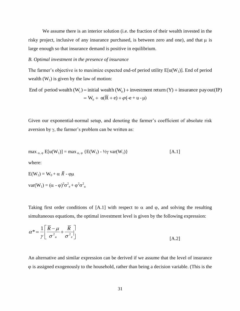
B. Optimal investment in the presence of insurance

The farmer’s objective is to maximize expected end-of period utility E[u(W1)]. End of period

wealth (W1) is given by the law of motion:

Given our exponential-normal setup, and denoting the farmer’s coefficient of absolute risk

aversion by , the farmer’s problem can be written as:

max , E[u(W1)] = max , {E(W1) - ½ var(W1)} [A.1]

where:

E(W1) = W0 + -

var(W1) = ( - )22e + 22

u

Taking first order conditions of [A.1] with respect to and , and solving the resulting

simultaneous equations, the optimal investment level is given by the following expression:

[A.2]

An alternative and similar expression can be derived if we assume that the level of insurance

is assigned exogenously to the household, rather than being a decision variable. (This is the

μ) - u + (-e e)Rα( W

(IP)payout insurance (Y) return investment )(W wealthinitial )(W wealthperiod of End

0

01

eu

RR22

1*

32

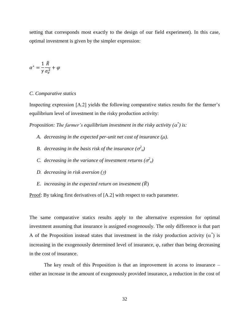
setting that corresponds most exactly to the design of our field experiment). In this case,

optimal investment is given by the simpler expression:

C. Comparative statics

Inspecting expression [A.2] yields the following comparative statics results for the farmer’s

equilibrium level of investment in the risky production activity:

Proposition: The farmer’s equilibrium investment in the risky activity (*) is:

A. decreasing in the expected per-unit net cost of insurance ().

B. decreasing in the basis risk of the insurance (2u)

C. decreasing in the variance of investment returns (2e)

D. decreasing in risk aversion ()

E. increasing in the expected return on investment ( )

Proof: By taking first derivatives of [A.2] with respect to each parameter.

The same comparative statics results apply to the alternative expression for optimal

investment assuming that insurance is assigned exogenously. The only difference is that part

A of the Proposition instead states that investment in the risky production activity (*) is

increasing in the exogenously determined level of insurance, , rather than being decreasing

in the cost of insurance.

The key result of this Proposition is that an improvement in access to insurance –

either an increase in the amount of exogenously provided insurance, a reduction in the cost of

33

the insurance, or an improvement in the quality of the insurance while keeping the cost fixed

– increases investment in the risky activity.

The simple intuition for these results is that the farmer’s optimal level of investment

trades off the high expected return of the investment against its risk. Improving access to

insurance against production risk allows the farmer to reduce the background risk associated

with any given investment level (i.e. to shift this risk-return frontier outwards), allowing the

farmer to invest more in equilibrium. Given these results, it is also straightforward to verify

that the farmer’s expected income and expected utility are decreasing in the expected per-

unit net cost of insurance (), and the basis risk of the insurance (2u), so that improving

access to insurance increases expected income and welfare.

Note that since we assume exponential utility, there are no wealth effects in the model

presented here. In reality, provision of insurance may affect behavior both through its risk-

management benefits and because it increases household wealth. To control for this, in our

field work we compare two groups, one of which receives insurance for free, the other of

which is promised the actuarial value of the insurance for free. In other words we effectively

hold fixed the wealth of the household between the treatment and control groups.

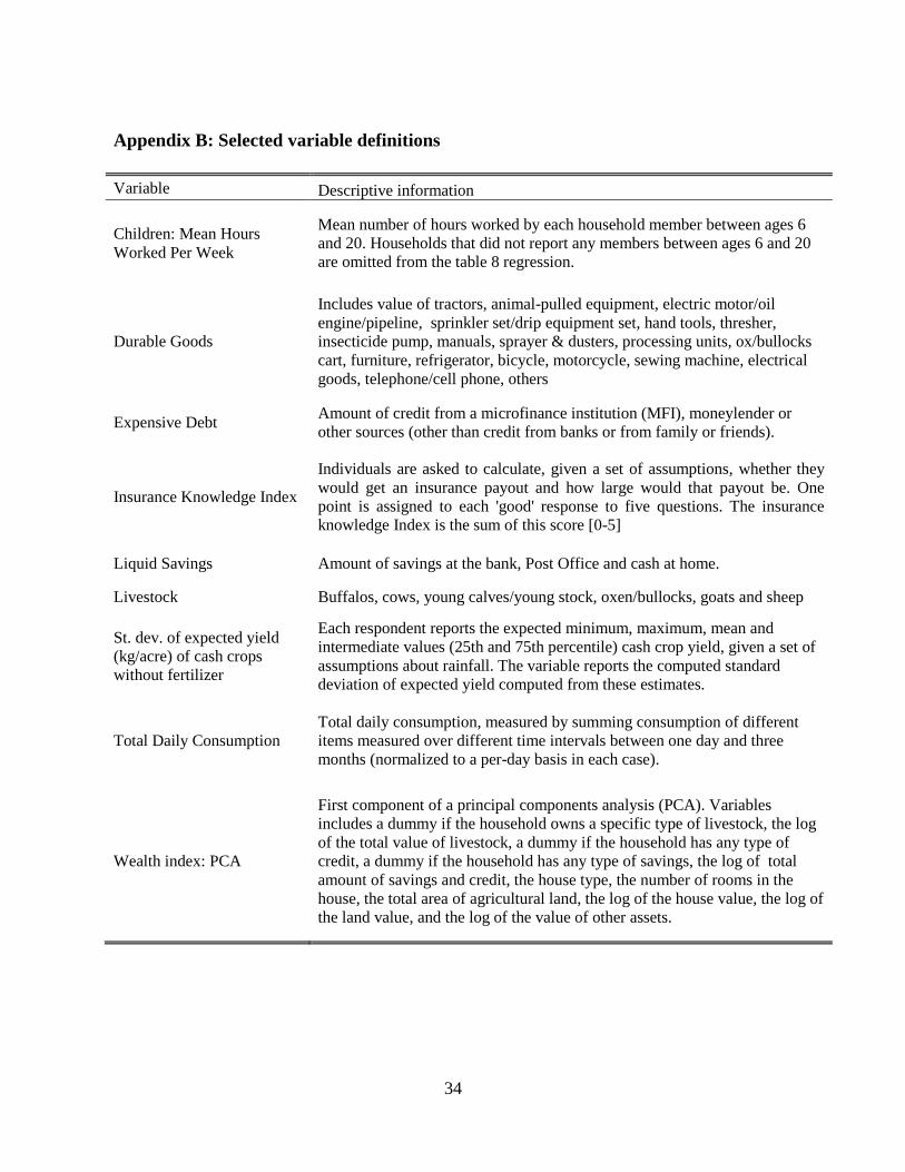
34

Appendix B: Selected variable definitions

Variable Descriptive information

Children: Mean Hours

Worked Per Week

Mean number of hours worked by each household member between ages 6

and 20. Households that did not report any members between ages 6 and 20

are omitted from the table 8 regression.

Durable Goods

Includes value of tractors, animal-pulled equipment, electric motor/oil

engine/pipeline, sprinkler set/drip equipment set, hand tools, thresher,

insecticide pump, manuals, sprayer & dusters, processing units, ox/bullocks

cart, furniture, refrigerator, bicycle, motorcycle, sewing machine, electrical

goods, telephone/cell phone, others

Expensive Debt Amount of credit from a microfinance institution (MFI), moneylender or

other sources (other than credit from banks or from family or friends).

Insurance Knowledge Index

Individuals are asked to calculate, given a set of assumptions, whether they

would get an insurance payout and how large would that payout be. One

point is assigned to each 'good' response to five questions. The insurance

knowledge Index is the sum of this score [0-5]

Liquid Savings Amount of savings at the bank, Post Office and cash at home.

Livestock Buffalos, cows, young calves/young stock, oxen/bullocks, goats and sheep

St. dev. of expected yield

(kg/acre) of cash crops

without fertilizer

Each respondent reports the expected minimum, maximum, mean and

intermediate values (25th and 75th percentile) cash crop yield, given a set of

assumptions about rainfall. The variable reports the computed standard

deviation of expected yield computed from these estimates.

Total Daily Consumption

Total daily consumption, measured by summing consumption of different

items measured over different time intervals between one day and three

months (normalized to a per-day basis in each case).

Wealth index: PCA

First component of a principal components analysis (PCA). Variables

includes a dummy if the household owns a specific type of livestock, the log

of the total value of livestock, a dummy if the household has any type of

credit, a dummy if the household has any type of savings, the log of total

amount of savings and credit, the house type, the number of rooms in the

house, the total area of agricultural land, the log of the house value, the log of

the land value, and the log of the value of other assets.

35

Figure 1: Timeline

Oct- Nov 2009

Household visit:

- Short baseline survey- Scratch-card

Follow-up Survey I:

investment

Jun-Jul 2009

Dec 2009 Jan 2010

Planting and Investment Decision

Harvest time

PayoutsMade

Apr-Jul 2010

Follow-up Survey II:

assets, consumption

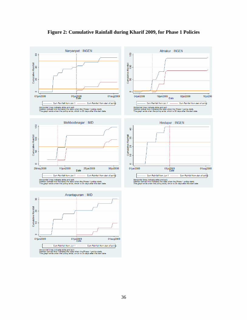
36

Figure 2: Cumulative Rainfall during Kharif 2009, for Phase 1 Policies

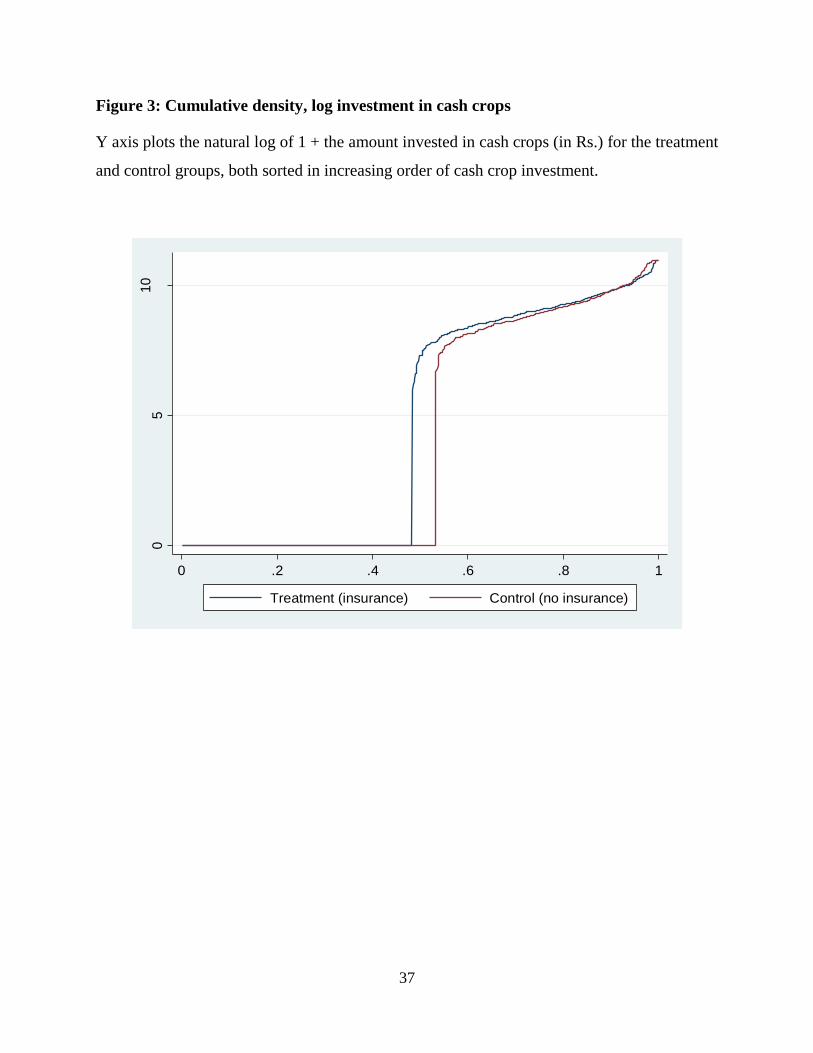
37

Figure 3: Cumulative density, log investment in cash crops

Y axis plots the natural log of 1 + the amount invested in cash crops (in Rs.) for the treatment

and control groups, both sorted in increasing order of cash crop investment.

05

10

0 .2 .4 .6 .8 1

Treatment (insurance) Control (no insurance)

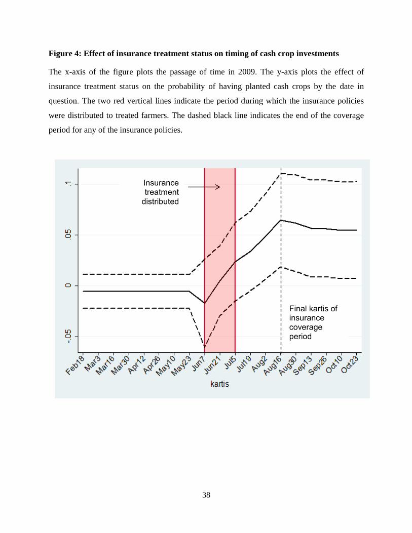
38

Figure 4: Effect of insurance treatment status on timing of cash crop investments

The x-axis of the figure plots the passage of time in 2009. The y-axis plots the effect of

insurance treatment status on the probability of having planted cash crops by the date in

question. The two red vertical lines indicate the period during which the insurance policies

were distributed to treated farmers. The dashed black line indicates the end of the coverage

period for any of the insurance policies.

Final kartis of insurance coverage period

Insurance treatment

distributed

Variable N Mean SD p10 p50 p90

A. Demographic CharacteristicsHousehold size 1,479 5.35 2.28 3 5 8Number of children 6 years old or younger 1,479 0.20 0.54 0 0 1Number of children 18 years old or younger 1,479 1.70 1.51 0 2 4Age of household head (Years) 1,479 49.60 12.40 35 50 65Highest level of schooling completed by HH (Years) 1,479 3.75 4.76 0 0 11Household head is unschooled (1 = "Yes") 1,479 0.54 0.50Household head able to read (1 = "Yes") 1,479 0.44 0.50

B. Livestock (as of June 2009)No. of large animals owned, i.e. buffalos, cows and oxen 1,479 2.25 3.01 0 2 6No. small animals owned, i.e. goats, sheep, chicken, pigs 1,479 5.23 22.22 0 0 10Total market value of livestock owned (Rs.) 1,479 34,263 58,623 0 20,000 80,000

C. Savings and CreditTotal amount of savings, all sources (Rs.) 1,479 21,353 29,472 0 11,000 56,980 Amount of savings with bank or post office (Rs.) 1,479 1,575 5,640 0 0 4,000 Amount of savings in cash at home (Rs.) 1,479 1,715 3,228 0 600 5,000 Amount of savings in jewelry (Rs.) 1,479 13,335 20,589 0 5,000 32,000 Amount of savings with SHG or other group (Rs.) 1,479 2,152 4,910 0 720 5,000 Amount of other savings (Rs.) 1,479 2,576 11,427 0 0 3,600

Total amount of credit owed, all sources (Rs.) 1,479 41,644 50,498 8,000 29,000 87,000 Amount of credit from bank (Rs.) 1,479 20,414 31,823 0 15,000 45,000 Amount of credit from family and friends (Rs.) 1,479 6,406 19,505 0 0 20,000 Amount of credit from MFIs (Rs.) 1,479 692 3,684 0 0 0 Amount of credit from moneylenders (Rs.) 1,479 12,747 30,840 0 0 35,000 Amount of credit from other sources of credit (Rs.) 1,479 1,386 5,079 0 0 5,000

D. Other AssetsHouse type: strong structure (1 = "Yes") 1,479 0.54 0.50House type: semi-strong structure (1 = "Yes") 1,479 0.33 0.47House type: weak structure (1 = "Yes") 1,479 0.13 0.33Number of rooms in the house 1,479 2.63 1.34 1 2 4Estimated value of the house if owned (Rs.) 1,479 117,221 165,962 25,000 70,000 220,000Total area of agricultural land (Acres) 1,479 5.37 5.47 2 4 10Estimated value of agricultural land (Rs.) 1,479 508,519 1,463,349 70,000 240,000 980,000Est. value of non-agricultural land and other assets (Rs.) 1,479 8,642 49,500 0 0 20,000

E. Other Variables of Interest:Wealth Index (PCA) 1,479 0 1.7 -2.1 0.03 2.07St. dev. of expected cash crop yield (kg/acre) 1,479 46.22 38.05 14.14 35.36 88.25Insurance knowledge at the baseline (0-5) 1,479 1.73 2.12 0 0 5Household head has heard of rainfall insurance (1 = "Yes") 1,479 0.42 0.49

Table 1: Household Summary Statistics

Notes: This table reports the summary statistics for the sample, which includes the 1479 individuals thatparticipated in both the baseline and follow-up surveys. The variables reported in Section C and E were collectedduring the baseline survey conducted between April and June 2009. Variables in Section A, B and D werecollected during the follow up survey in November 2009, but respondents were asked to report answers as of June2009. See Appendix Table A2 for variable definitions.

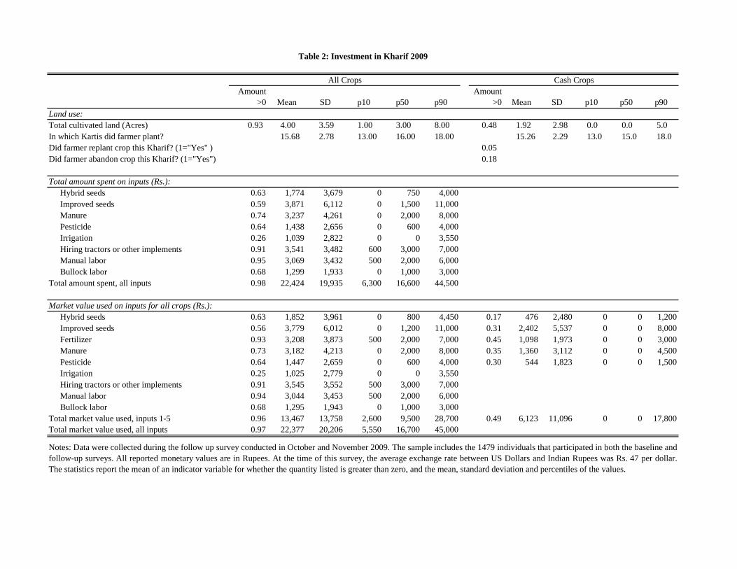
Amount >0 Mean SD p10 p50 p90

Amount >0 Mean SD p10 p50 p90

Land use:Total cultivated land (Acres) 0.93 4.00 3.59 1.00 3.00 8.00 0.48 1.92 2.98 0.0 0.0 5.0In which Kartis did farmer plant? 15.68 2.78 13.00 16.00 18.00 15.26 2.29 13.0 15.0 18.0Did farmer replant crop this Kharif? (1="Yes" ) 0.05Did farmer abandon crop this Kharif? (1="Yes") 0.18

Total amount spent on inputs (Rs.):Hybrid seeds 0.63 1,774 3,679 0 750 4,000Improved seeds 0.59 3,871 6,112 0 1,500 11,000Manure 0.74 3,237 4,261 0 2,000 8,000Pesticide 0.64 1,438 2,656 0 600 4,000Irrigation 0.26 1,039 2,822 0 0 3,550Hiring tractors or other implements 0.91 3,541 3,482 600 3,000 7,000Manual labor 0.95 3,069 3,432 500 2,000 6,000Bullock labor 0.68 1,299 1,933 0 1,000 3,000

Total amount spent, all inputs 0.98 22,424 19,935 6,300 16,600 44,500

Market value used on inputs for all crops (Rs.):Hybrid seeds 0.63 1,852 3,961 0 800 4,450 0.17 476 2,480 0 0 1,200Improved seeds 0.56 3,779 6,012 0 1,200 11,000 0.31 2,402 5,537 0 0 8,000Fertilizer 0.93 3,208 3,873 500 2,000 7,000 0.45 1,098 1,973 0 0 3,000Manure 0.73 3,182 4,213 0 2,000 8,000 0.35 1,360 3,112 0 0 4,500Pesticide 0.64 1,447 2,659 0 600 4,000 0.30 544 1,823 0 0 1,500Irrigation 0.25 1,025 2,779 0 0 3,550Hiring tractors or other implements 0.91 3,545 3,552 500 3,000 7,000Manual labor 0.94 3,044 3,453 500 2,000 6,000Bullock labor 0.68 1,295 1,943 0 1,000 3,000

Total market value used, inputs 1-5 0.96 13,467 13,758 2,600 9,500 28,700 0.49 6,123 11,096 0 0 17,800Total market value used, all inputs 0.97 22,377 20,206 5,550 16,700 45,000

Table 2: Investment in Kharif 2009

All Crops Cash Crops

Notes: Data were collected during the follow up survey conducted in October and November 2009. The sample includes the 1479 individuals that participated in both the baseline andfollow-up surveys. All reported monetary values are in Rupees. At the time of this survey, the average exchange rate between US Dollars and Indian Rupees was Rs. 47 per dollar.The statistics report the mean of an indicator variable for whether the quantity listed is greater than zero, and the mean, standard deviation and percentiles of the values.

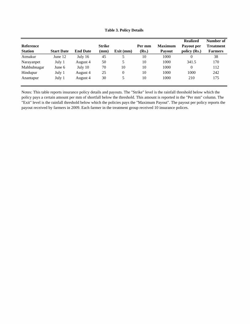
Reference Station Start Date End Date

Strike (mm) Exit (mm)

Per mm (Rs.)

Maximum Payout

Realized Payout per policy (Rs.)

Number of Treatment Farmers

Atmakur June 12 July 16 45 5 10 1000 0 38Narayanpet July 1 August 4 50 5 10 1000 341.5 170Mahbubnagar June 6 July 10 70 10 10 1000 0 112Hindupur July 1 August 4 25 0 10 1000 1000 242Anantapur July 1 August 4 30 5 10 1000 210 175

Notes: This table reports insurance policy details and payouts. The "Strike" level is the rainfall threshold below which the policy pays a certain amount per mm of shortfall below the threshold. This amount is reported in the "Per mm" column. The "Exit" level is the rainfall threshold below which the policies pays the "Maximum Payout". The payout per policy reports the payout received by farmers in 2009. Each farmer in the treatment group received 10 insurance polices.

Table 3. Policy Details

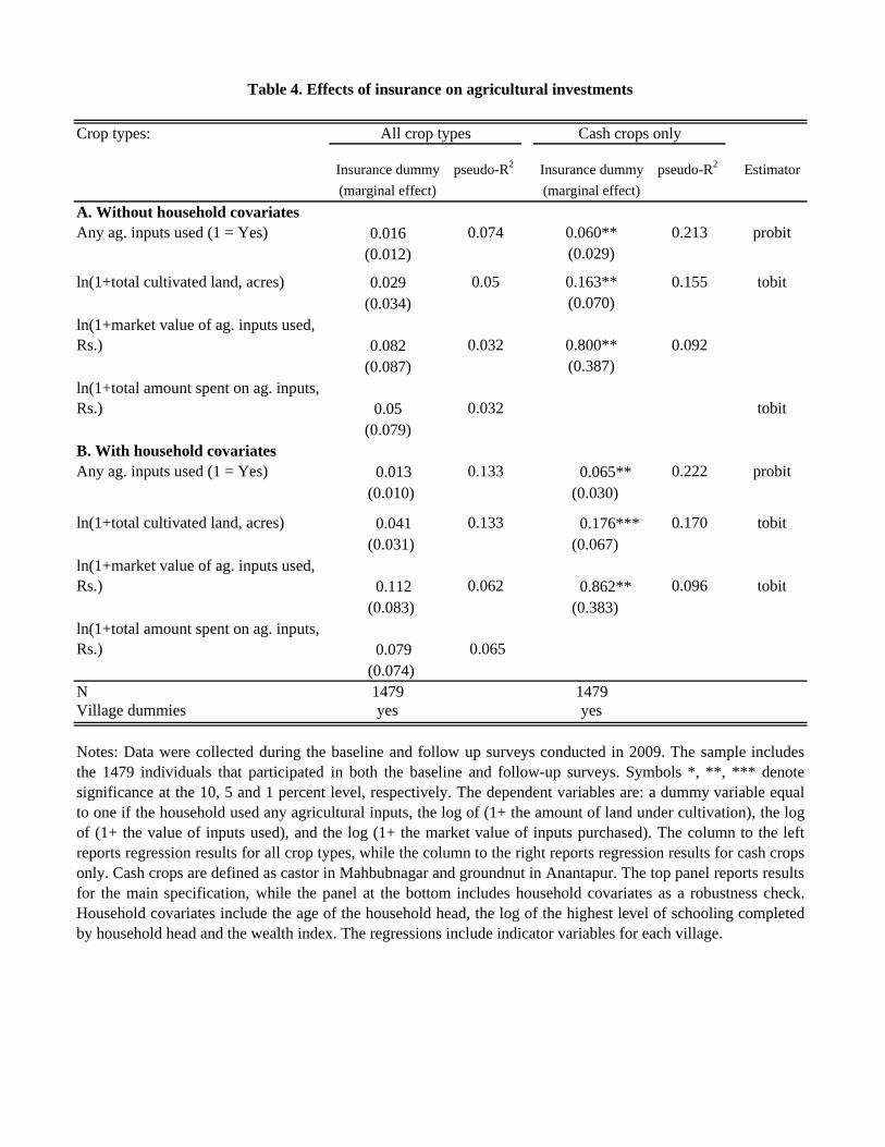
Crop types:

Insurance dummy pseudo-R2 Insurance dummy pseudo-R2 Estimator

(marginal effect) (marginal effect)

Any ag. inputs used (1 = Yes) 0.016 0.074 0.060** 0.213 probit(0.012) (0.029)

ln(1+total cultivated land, acres) 0.029 0.05 0.163** 0.155 tobit(0.034) (0.070)

ln(1+market value of ag. inputs used, Rs.) 0.082 0.032 0.800** 0.092

(0.087) (0.387)ln(1+total amount spent on ag. inputs, Rs.) 0.05 0.032 tobit

(0.079)

Any ag. inputs used (1 = Yes) 0.013 0.133 0.065** 0.222 probit (0.010) (0.030)

ln(1+total cultivated land, acres) 0.041 0.133 0.176*** 0.170 tobit (0.031) (0.067)

ln(1+market value of ag. inputs used, Rs.) 0.112 0.062 0.862** 0.096 tobit

(0.083) (0.383) ln(1+total amount spent on ag. inputs, Rs.) 0.079 0.065

(0.074) N 1479 1479Village dummies yes yes

Notes: Data were collected during the baseline and follow up surveys conducted in 2009. The sample includesthe 1479 individuals that participated in both the baseline and follow-up surveys. Symbols *, **, *** denotesignificance at the 10, 5 and 1 percent level, respectively. The dependent variables are: a dummy variable equalto one if the household used any agricultural inputs, the log of (1+ the amount of land under cultivation), the logof (1+ the value of inputs used), and the log (1+ the market value of inputs purchased). The column to the leftreports regression results for all crop types, while the column to the right reports regression results for cash cropsonly. Cash crops are defined as castor in Mahbubnagar and groundnut in Anantapur. The top panel reports resultsfor the main specification, while the panel at the bottom includes household covariates as a robustness check.Household covariates include the age of the household head, the log of the highest level of schooling completedby household head and the wealth index. The regressions include indicator variables for each village.

Table 4. Effects of insurance on agricultural investments

All crop types Cash crops only

A. Without household covariates

B. With household covariates

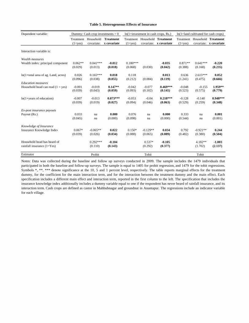
Dependent variable:

Treatment (1=yes)

Household covariate:

Treatment x covariate

Treatment (1=yes)

Household covariate:

Treatment x covariate

Treatment (1=yes)

Household covariate:

Treatment x covariate

Interaction variable is:

Wealth measuresWealth index: principal component 0.062** 0.041*** -0.012 0.180*** -0.035 0.871** 0.641*** -0.220

(0.029) (0.013) (0.018) (0.068) (0.030) (0.042) (0.388) (0.168) (0.235)

ln(1+total area of ag. Land, acres) 0.026 0.165*** 0.018 0.118 0.013 0.636 2.615*** 0.052 (0.096) (0.038) (0.055) (0.212) (0.084) (0.119) (1.241) (0.475) (0.666)

Education measuresHousehold head can read (1 = yes) -0.001 -0.019 0.147** -0.042 -0.077 0.469*** -0.048 -0.155 1.959**

(0.039) (0.043) (0.059) (0.093) (0.102) (0.141) (0.523) (0.575) (0.779)

ln(1+years of education) -0.007 -0.013 0.073*** -0.053 -0.04 0.218*** -0.128 -0.140 0.948*** (0.039) (0.019) (0.027) (0.094) (0.046) (0.063) (0.529) (0.259) (0.348)

Ex-post insurance payoutsPayout (Rs.) 0.033 na 0.000 0.076 na 0.000 0.333 na 0.001

(0.045) na (0.000) (0.098) na (0.000) (0.544) na (0.001)

Knowledge of InsuranceInsurance Knowledge Index 0.067* -0.065** 0.022 0.150* -0.129** 0.034 0.792 -0.921** 0.244

(0.039) (0.026) (0.034) (0.088) (0.065) (0.089) (0.482) (0.380) (0.504)

0.292*** -0.104 0.537* -0.105 4.182** -1.003 (0.110) (0.143) (0.292) (0.377) (1.702) (2.137)

Estimator

Notes: Data was collected during the baseline and follow up surveys conducted in 2009. The sample includes the 1479 individuals thatparticipated in both the baseline and follow-up surveys. The sample is equal to 1405 for probit regression, and 1479 for the tobit regressions.Symbols *, **, *** denote significance at the 10, 5 and 1 percent level, respectively. The table reports marginal effects for the treatmentdummy, for the coefficient for the main interaction term, and for the interaction between the treatment dummy and the main effect. Eachspecification includes a different main effect and interaction term, reported in the first column to the left. The specification that includes theinsurance knowledge index additionally includes a dummy variable equal to one if the respondent has never heard of rainfall insurance, and itsinteraction term. Cash crops are defined as castor in Mahbubnagar and groundnut in Anantapur. The regressions include an indicator variablefor each village.

Table 5. Heterogeneous Effects of Insurance

Dummy: Cash crop investments > 0 ln(1+investment in cash crops, Rs.) ln(1+land cultivated for cash crops)

Probit Tobit Tobit

Household head has heard of rainfall insurance (1=Yes)

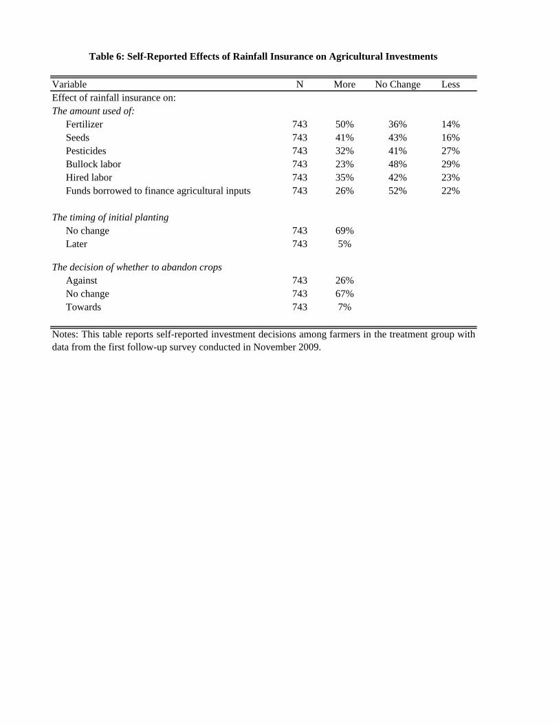
Variable N More No Change LessEffect of rainfall insurance on:The amount used of:

Fertilizer 743 50% 36% 14%Seeds 743 41% 43% 16%Pesticides 743 32% 41% 27%Bullock labor 743 23% 48% 29%Hired labor 743 35% 42% 23%Funds borrowed to finance agricultural inputs 743 26% 52% 22%

The timing of initial plantingNo change 743 69%Later 743 5%

The decision of whether to abandon cropsAgainst 743 26%No change 743 67%Towards 743 7%

Table 6: Self-Reported Effects of Rainfall Insurance on Agricultural Investments

Notes: This table reports self-reported investment decisions among farmers in the treatment group withdata from the first follow-up survey conducted in November 2009.

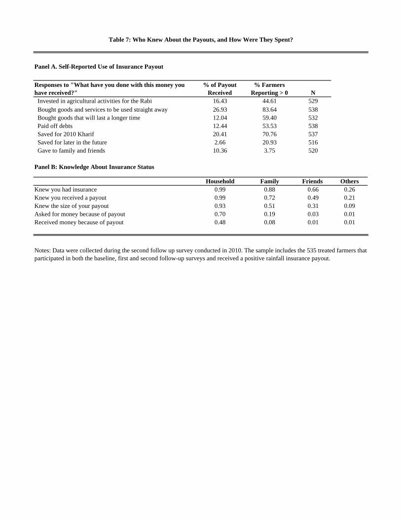
Panel A. Self-Reported Use of Insurance Payout

Invested in agricultural activities for the Rabi 16.43 44.61 529 Bought goods and services to be used straight away 26.93 83.64 538 Bought goods that will last a longer time 12.04 59.40 532 Paid off debts 12.44 53.53 538 Saved for 2010 Kharif 20.41 70.76 537 Saved for later in the future 2.66 20.93 516 Gave to family and friends 10.36 3.75 520

Panel B: Knowledge About Insurance Status

Household Family Friends OthersKnew you had insurance 0.99 0.88 0.66 0.26Knew you received a payout 0.99 0.72 0.49 0.21Knew the size of your payout 0.93 0.51 0.31 0.09Asked for money because of payout 0.70 0.19 0.03 0.01Received money because of payout 0.48 0.08 0.01 0.01

Notes: Data were collected during the second follow up survey conducted in 2010. The sample includes the 535 treated farmers that participated in both the baseline, first and second follow-up surveys and received a positive rainfall insurance payout.

Table 7: Who Knew About the Payouts, and How Were They Spent?

Responses to "What have you done with this money you have received?"

% of Payout Received

% Farmers Reporting > 0 N

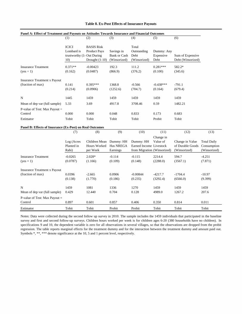
Panel A: Effect of Treatment and Payouts on Attitudes Towards Insurance and Financial Outcomes(1) (2) (3) (4) (5) (6)

ICICI Lombard is trustworthy (1-10)

BASIS Risk Product Pays Out During Drought (1-10)

Savings in Bank or Cash (Winsorized)

Total Outstanding Debt (Winsorized)

Dummy: Any Expensive Debt

Sum of Expensive Debt (Winsorized)

Insurance Treatment 0.371** -0.00423 192.3 111.2 0.281*** 582.2*(yes = 1) (0.162) (0.0487) (866.9) (376.2) (0.100) (345.6)

Insurance Treatment x Payout (fraction of max) 0.141 0.395*** 1368.8 -0.566 -0.438*** -791.1

(0.214) (0.0906) (1252.6) (704.7) (0.164) (679.4)

N 1445 1459 1459 1459 1459 1459

Mean of dep var (full sample) 5.33 3.69 4917.8 3708.46 0.59 1482.21

P-value of Test: Max Payout = Control 0.000 0.000 0.048 0.833 0.173 0.683

Estimator Tobit Tobit Tobit Tobit Probit Tobit

Panel B: Effects of Inusrance (Ex-Post) on Real Outcomes(7) (8) (9) (10) (11) (12) (13)

Log (Acres Planted in Rabi)

Children Mean Hours Worked per Week

Dummy: HH Has NREGA Earnings

Dummy: HH Earned Income from Migration

Change in Value of Livestock (Winsorized)

Change in Value of Durable Goods (Winsorized)

Total Daily Consumption (Winsorized)

Insurance Treatment -0.0265 2.028* -0.114 -0.115 2214.4 594.7 -4.251(yes = 1) (0.0787) (1.166) (0.109) (0.148) (2288.0) (3567.1) (7.871)

Insurance Treatment x Payout (fraction of max) 0.0396 -2.665 0.0906 -0.00844 -4217.7 -1704.4 -10.97

(0.138) (1.770) (0.186) (0.235) (3292.4) (6566.0) (9.399)

N 1459 1081 1336 1270 1459 1459 1459Mean of dep var (full sample) 0.429 12.440 0.704 0.128 4989.0 1267.2 207.6

P-value of Test: Max Payout = Control 0.897 0.601 0.857 0.406 0.350 0.814 0.011

Estimator Tobit Tobit Probit Probit Tobit Tobit Tobit

Table 8. Ex-Post Effects of Insurance Payouts

Notes: Data were collected during the second follow up survey in 2010. The sample includes the 1459 individuals that participated in the baselinesurvey and first and second follow-up surveys. Children hours worked per week is for children ages 6-20 (380 households have no children). Inspecifications 9 and 10, the dependent variable is zero for all observations in several villages, so that the observations are dropped from the probitregression. The table reports marginal effects for the treatment dummy and for the interaction between the treatment dummy and amount paid out.Symbols *, **, *** denote significance at the 10, 5 and 1 percent level, respectively.

   

 

 

 

 

Online Appendix for

How Does Risk Management Influence Production Decisions?

Evidence from a Field Experiment

Table OA1: Test of Balance

Table OA2: Cash Crop Treatment Disaggregated by Investment Type

Table OA3: Treatment Effects, Winsorized at Two Percent Level

Table OA4: Treatment Effects with Linear Probability Model

Table OA5: Summary Statistics for 2010 Followup Survey

Variable NTreatment

MeanControl Mean Difference

Robust p-value

Significance Level

A. Demographic Characteristics Household size 1,479 5.32 5.38 -0.06 0.60Number of children 6 years old or younger 1,479 0.19 0.20 -0.01 0.72Number of children 18 years old or younger 1,479 1.67 1.72 -0.05 0.49Age of household head (Years) 1,470 49.82 49.37 0.45 0.49Highest level of schooling completed by household head (Years) 1,479 3.62 3.77 -0.15 0.54Household head is unschooled (1 = "Yes") 1,479 0.56 0.54 0.02 0.32Household head able to read (1 = "Yes") 1,479 0.42 0.44 -0.02 0.37Household head able to write (1 = "Yes") 1,479 0.38 0.41 -0.03 0.25

B. Savings and CreditTotal amount of savings, all sources (Rs.) 1,479 22,093 20,607 1,486 0.33 Amount of savings with bank or post office (Rs.) 1,479 1,735 1,413 322.08 0.27 Amount of savings in cash at home (Rs.) 1,479 1,832 1,597 235.10 0.16 Amount of savings in jewelry (Rs.) 1,479 13,275 13,396 -121.77 0.91 Amount of savings with SHG or other group (Rs.) 1,479 2,186 2,117 68.39 0.79 Amount of other savings (Rs.) 1,479 3,065 2,083 982.04 0.10 *Total amount of credit owed, all sources (Rs.) 1,479 41,320 41,972 -652.13 0.80 Amount of credit from bank (Rs.) 1,479 21,168 19,652 1,516 0.36 Amount of credit from family and friends (Rs.) 1,479 6,810 5,998 812.19 0.42 Amount of credit from MFIs (Rs.) 1,479 557.87 827.45 -269.58 0.16 Amount of credit from moneylenders (Rs.) 1,479 11,505 14,000 -2,496 0.12 Amount of credit from other sources of credit (Rs.) 1,479 1,279 1,494 -215.29 0.42

C. Livestock and other Assets (as of June 2009)Number of large animals owned, i.e. buffalos, cows and oxen 1,479 2.22 2.29 -0.07 0.64Number of small animals owned, i.e. goats, sheep, chicken, pigs 1,479 4.70 5.77 -1.07 0.36Total market value of livestock owned (Rs.) 1,479 31,922 36,626 -4,704 0.12House type: strong structure (1 = "Yes") 1,479 0.54 0.55 -0.01 0.65House type: semi-strong structure (1 = "Yes") 1,479 0.33 0.32 0.01 0.67House type: weak structure (1 = "Yes") 1,479 0.13 0.12 0.01 0.81Number or rooms in the house 1,479 2.62 2.65 -0.03 0.72Estimated value of the house if owned (Rs.) 1,479 116,938 117,346 -407.42 0.96

(cont. following page)

Table OA1: Test of Balance

Variable NTreatment

MeanControl Mean Difference

Robust p-value Sig. Level

C. Livestock and other Assets (as of June 2009) contd.Total area of agricultural land (Acres) 1,479 5.44 5.29 0.15 0.59Estimated value of agricultural land (Rs.) 1,479 558,434 457,887 100,547 0.19Estimated value of non-agricultural land and other houses (Rs.) 1,479 6,677 10,615 -3,938 0.13

D. Agricultural InvestmentsTotal cultivated land (Acres) - all crops during Kharif'08 1,479 4.38 4.24 0.14 0.50Total cultivated land (Acres) - cash crops during Kharif'08 1,479 3.48 3.32 0.16 0.27Any land planted - cash crops during Kharif'08 (1 = Yes) 1,479 0.92 0.92 0.00 0.66Total amount spent on inputs - all crops during Kharif'08 1,479 20,036 20,115 -78.51 0.94

Amount spent on hybrid seeds - all crops during Kharif'08 1,479 853.28 844.28 9.00 0.94Amount spent on improved seeds - all crops during Kharif'08 1,479 4,374 4,356 18.58 0.96Amount spent on fertilizer - all crops during Kharif'08 1,479 3,287 3,267 20.47 0.92Amount spent on manure - all crops during Kharif'08 1,479 2,073 2,339 -266.07 0.10Amount spent on irrigation - all crops during Kharif'08 1,479 119.64 181.66 -62.02 0.18Amount spent on hiring tractor/other impl - all crops during Kharif'08 1,479 2,723 2,635 88.07 0.64Amount spent on manual labor - all crops during Kharif'08 1,479 5,028 4,896 132.35 0.63Amount spent on bullock labor - all crops during Kharif'08 1,479 1,578 1,597 -18.90 0.88

Total amount spent on inputs - cash crops during Kharif'08 1,479 15,868 15,923 -54.52 0.94Amount spent on hybrid seeds - cash crops during Kharif'08 1,479 454.99 427.08 27.91 0.61Amount spent on improved seeds - cash crops during Kharif'08 1,479 4,012 3,969 42.30 0.89Amount spent on fertilizer - cash crops during Kharif'08 1,479 2,284 2,302 -17.67 0.88Amount spent on manure - cash crops during Kharif'08 1,479 1,754 1,928 -174.63 0.24Amount spent on irrigation - cash crops during Kharif'08 1,479 22.53 40.23 -17.70 0.29Amount spent on hiring tractor/other impl - cash crops during Kharif'08 1,479 2,083 1,960 123.08 0.28Amount spent on manual labor - cash crops during Kharif'08 1,479 3,866 3,884 -18.55 0.93Amount spent on bullock labor - cash crops during Kharif'08 1,479 1,392 1,412 -19.27 0.86

Notes: The table reports a randomization test run on the baseline sample, where each variable is tested for treatment assignment OLS estimation,robust standard errors. Symbols *, **, *** denote significance at the 10, 5 and 1 percent level, respectively. An F-test confirms that the variables arejointly insignificant: the F-statistic is 0.83, and the corresponding p-values is 0.7896.

Table OA1: Test of Balance (Continued)

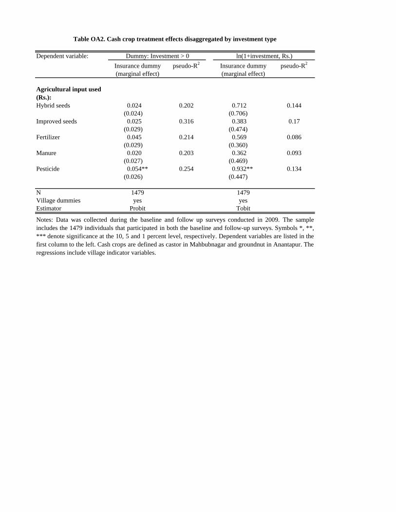
Dependent variable:

Insurance dummy pseudo-R2 Insurance dummy pseudo-R2

(marginal effect) (marginal effect)

Agricultural input used (Rs.):Hybrid seeds 0.024 0.202 0.712 0.144

(0.024) (0.706) Improved seeds 0.025 0.316 0.383 0.17

(0.029) (0.474) Fertilizer 0.045 0.214 0.569 0.086

(0.029) (0.360) Manure 0.020 0.203 0.362 0.093

(0.027) (0.469) Pesticide 0.054** 0.254 0.932** 0.134

(0.026) (0.447)

N 1479 1479Village dummies yes yesEstimator Probit Tobit

Notes: Data was collected during the baseline and follow up surveys conducted in 2009. The sampleincludes the 1479 individuals that participated in both the baseline and follow-up surveys. Symbols *, **,*** denote significance at the 10, 5 and 1 percent level, respectively. Dependent variables are listed in thefirst column to the left. Cash crops are defined as castor in Mahbubnagar and groundnut in Anantapur. Theregressions include village indicator variables.

Table OA2. Cash crop treatment effects disaggregated by investment type

Dummy: Investment > 0 ln(1+investment, Rs.)

Crop types:

Insurance dummy pseudo-R2 Insurance dummy pseudo-R2 Estimator(marginal effect) (marginal effect)

Any ag. inputs used (1 = Yes) 0.016 0.074 0.060** 0.213 probit (0.012) (0.029)

ln(1+total cultivated land, acres) 0.030 0.050 0.162** 0.156 tobit (0.034) (0.068)

ln(1+market value of ag. inputs used, Rs.) 0.088 0.032 0.808** 0.092 tobit (0.087) (0.387)

ln(1+total amount spent on ag. inputs, Rs.) (0.078) 0.031 tobit (0.078)

Any ag. inputs used (1 = Yes) 0.013 0.074 0.065** 0.213 probit (0.010) (0.030)

ln(1+total cultivated land, acres) 0.042 0.050 0.175*** 0.156 tobit (0.031) (0.066)

ln(1+market value of ag. inputs used, Rs.) 0.118 0.032 0.869** 0.092 tobit (0.083) (0.383)

ln(1+total amount spent on ag. inputs, Rs.) 0.085 0.031 (0.074)

N 1479 1479Village dummies yes yes

Notes: Data were collected during the baseline and follow up surveys conducted in 2009. The sample includes the 1479individuals that participated in both the baseline and follow-up surveys. Symbols *, **, *** denote significance at the 10, 5and 1 percent level, respectively. The dependent variables are: a dummy variable equal to one if the household used anyagricultural inputs, the log of (1+ the amount of land under cultivation), the log of (1+ the value of inputs used), and the log(1+ the market value of inputs purchased). The column to the left reports regression results for all crop types, while thecolumn to the right reports regression results for cash crops only. Cash crops are defined as castor in Mahbubnagar andgroundnut in Anantapur. The top panel reports results for the main specification, while the panel at the bottom includeshousehold covariates as a robustness check. Household covariates included in this specification are the age of the householdhead, the log of the highest level of schooling completed by household head and the wealth index. The regressions includeindicator variables for each village.

Table OA3. Treatment Effects, Winsorized Two Percent

All crop types Cash crops only

A. Without household covariates

B. With household covariates

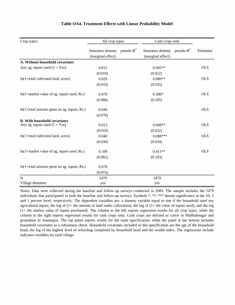
Crop types:

Insurance dummy pseudo-R2 Insurance dummy pseudo-R2 Estimator

(marginal effect) (marginal effect)

Any ag. inputs used (1 = Yes) 0.012 0.045** OLS

(0.010) (0.022)

ln(1+total cultivated land, acres) 0.029 0.080** OLS

(0.033) (0.035)

ln(1+market value of ag. inputs used, Rs.) 0.079 0.380* OLS

(0.086) (0.195)

ln(1+total amount spent on ag. inputs, Rs.) 0.049 OLS

(0.078)

Any ag. inputs used (1 = Yes) 0.013 0.048** OLS

(0.010) (0.022)

ln(1+total cultivated land, acres) 0.040 0.088*** OLS

(0.030) (0.034)

ln(1+market value of ag. inputs used, Rs.) 0.109 0.411** OLS

(0.082) (0.193)

ln(1+total amount spent on ag. inputs, Rs.) 0.078

(0.074)

N 1479 1479Village dummies yes yes

Notes: Data were collected during the baseline and follow up surveys conducted in 2009. The sample includes the 1479individuals that participated in both the baseline and follow-up surveys. Symbols *, **, *** denote significance at the 10, 5and 1 percent level, respectively. The dependent variables are: a dummy variable equal to one if the household used anyagricultural inputs, the log of (1+ the amount of land under cultivation), the log of (1+ the value of inputs used), and the log(1+ the market value of inputs purchased). The column to the left reports regression results for all crop types, while thecolumn to the right reports regression results for cash crops only. Cash crops are defined as castor in Mahbubnagar andgroundnut in Anantapur. The top panel reports results for the main specification, while the panel at the bottom includeshousehold covariates as a robustness check. Household covariates included in this specification are the age of the householdhead, the log of the highest level of schooling completed by household head and the wealth index. The regressions includeindicator variables for each village.

Table OA4. Treatment Effects with Linear Probability Model

All crop types Cash crops only

A. Without household covariates

B. With household covariates

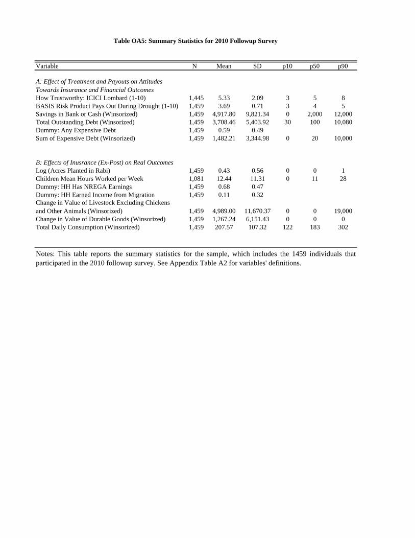
Variable N Mean SD p10 p50 p90

A: Effect of Treatment and Payouts on Attitudes Towards Insurance and Financial OutcomesHow Trustworthy: ICICI Lombard (1-10) 1,445 5.33 2.09 3 5 8BASIS Risk Product Pays Out During Drought (1-10) 1,459 3.69 0.71 3 4 5Savings in Bank or Cash (Winsorized) 1,459 4,917.80 9,821.34 0 2,000 12,000Total Outstanding Debt (Winsorized) 1,459 3,708.46 5,403.92 30 100 10,080Dummy: Any Expensive Debt 1,459 0.59 0.49Sum of Expensive Debt (Winsorized) 1,459 1,482.21 3,344.98 0 20 10,000

B: Effects of Inusrance (Ex-Post) on Real OutcomesLog (Acres Planted in Rabi) 1,459 0.43 0.56 0 0 1Children Mean Hours Worked per Week 1,081 12.44 11.31 0 11 28Dummy: HH Has NREGA Earnings 1,459 0.68 0.47Dummy: HH Earned Income from Migration 1,459 0.11 0.32Change in Value of Livestock Excluding Chickens and Other Animals (Winsorized) 1,459 4,989.00 11,670.37 0 0 19,000Change in Value of Durable Goods (Winsorized) 1,459 1,267.24 6,151.43 0 0 0Total Daily Consumption (Winsorized) 1,459 207.57 107.32 122 183 302

Table OA5: Summary Statistics for 2010 Followup Survey

Notes: This table reports the summary statistics for the sample, which includes the 1459 individuals thatparticipated in the 2010 followup survey. See Appendix Table A2 for variables' definitions.