How Did China’s WTO Entry Benefit U.S. Consumers?∗

Mary AmitiFederal Reserve Bank of New York

Mi DaiBeijing Normal Univesity

Robert C. FeenstraUniversity of California, Davis

John RomalisUniversity of Sydney

Preliminary

June 27, 2016

Abstract

China’s rapid rise in the global economy following its 2001 WTO entry has raised ques-

tions about its economic impact on the rest of the world. In this paper, we focus on the

U.S. market and potential consumer benefits. We find that the China trade shock reduced

the U.S. manufacturing price index by 7.3 percent between 2000 and 2006. In principle,

this consumer welfare gain could be driven by two distinct policy changes that occurred

with WTO entry. One, which has received much attention in the literature, is the U.S.

granting permanent normal trade relations (PNTR) to China, effectively removing the

threat of China facing very high tariffs on its exports to the U.S. Two, a new channel we

identify through which China’s WTO entry lowered U.S. price indexes, is China reduc-

ing its own input tariffs. Our results show that China’s lower input tariffs increased its

imported inputs, boosting Chinese firm’s productivity and their export values and va-

rieties. Lower input tariffs also reduced Chinese export prices to the U.S. market. In

contrast, PNTR only increased Chinese exports to the U.S. through its effect on new en-

try, but had no effect on Chinese productivity nor export prices. We find that at least two

thirds of the China WTO effect on U.S. price indexes was through China lowering its own

tariffs on intermediate inputs.∗Amiti: Federal Reserve Bank of New York. 33 Liberty Street, New York, NY 10045 (email: mary.amiti@ny.frb.org);

Di: School of Economics and Business Administration (SEBA), Beijing Normal University, Beijing 100875, China(email: daimi002@gmail.com); Feenstra: UC Davis (rcfeenstra@ucdavis.edu); Romalis: University of Sydney(john.romalis@sydney.edu.au. We thank Gordon Hanson, Pablo Fajgelbaum, Dan Trefler and David Weinstein for in-sightful comments. We are grateful to Tyler Bodine-Smith and Preston Mui for excellent research assistance. The viewsexpressed in this paper are those of the authors and do not necessarily represent those of the Federal Reserve Bank of NewYork or the Federal Reserve System.

1

1 Introduction

China’s manufacturing export growth in the last 20 years has produced a dramatic realignment of

world trade, with China emerging as the world’s largest exporter. China’s export growth was espe-

cially rapid following its World Trade Organization (WTO) entry in 2001, with the 2001–2006 growth

rate of 30 percent per annum being more than double the growth rate in the previous five years. This

growth has been so spectacular that it has attracted increasing attention to the negative effects of the

China “trade shock” on other countries, such as employment and wage losses in import-competing

U.S. manufacturing industries. Surprisingly, given the traditional focus of international trade theory,

little analysis has been made of the potential gains to consumers in the rest of the world, who could

benefit from access to cheaper Chinese imports and more imported varieties. Our focus is on poten-

tial benefits to consumers in the U.S., where China accounts for more than 20 percent of imports. In

principle, consumer gains could be driven by two distinct policy changes that occurred with China’s

WTO entry. One, which has received much attention in the literature, is the U.S. granting perma-

nent normal trade relations (PNTR) to China, effectively removing the threat of China facing very

high tariffs on its exports to the U.S. Two, a new channel we identify through which China’s WTO

entry lowered U.S. price indexes, is China reducing its own input tariffs. In this paper, we quantify

how much U.S. consumer welfare improved due to China’s WTO entry; and we identify that the key

mechanism by which China’s WTO entry reduced U.S. price indexes was through China lowering

its own tariffs on intermediate inputs.

To measure China’s impact on U.S. consumers (by which we mean both households and firms im-

porting from China), we utilize Chinese firm-product-destination level export data for the years 2000

to 2006, during which China’s exports to the U.S. increased nearly four-fold. One striking feature is

that the extensive margin of China’s U.S. exports accounts for 85 percent of this growth, and most of

it is due to new firms entering the export market (70 percent of total growth) rather than incumbents

exporting new products (15 percent of total growth). To ensure we properly incorporate new vari-

eties in measuring price indexes, we construct an exact CES price index, as in Feenstra (1994), which

comprises a “price” and a “variety” component.1 We find that the China import price index in the

U.S. falls by 44 percent over the period 2000 to 2006 due to the growth in exported product varieties.

But of course this number needs to be adjusted by China’s share in U.S. manufacturing industries to

get a measure of U.S. consumer welfare. We supplement the Chinese data with U.S. reported trade

data from other countries as well as U.S. domestic sales to construct overall U.S. manufacturing price

indexes. With these data, we explicitly take into account that the China shock can affect prices of

competitor firms as well as net entry in the U.S. market.

We model Chinese firm behavior by generalizing the Melitz (2003) model to allow firms to import

intermediate inputs as in Blaum, Lelarge, and Peters (2015). We expect that the reduction in China’s

1Broda and Weinstein (2006) built on this methodology to estimate the size of the gains from importing new vari-eties into the U.S. In contrast to that paper, we define a Chinese variety at the firm-product-destination level (rather thanproduct-country).

2

tariffs on intermediate inputs has expanded the international sourcing of these inputs, as in Antras,

Fort, and Tintelnot (2014), Gopinath and Neiman (2014), and Halpern, Koren, and Szeidl (2015).

Expanded sourcing of imported inputs raises Chinese firms’ productivity, which makes it possible for

them to increase their exports on both the intensive and extensive margins. Lower tariffs on Chinese

imported inputs also lowers the marginal costs of Chinese firms producing goods, thus reducing

export prices. We also extend the theory to allow the China shock to be driven by a reduction in

uncertainty due to PNTR, which we model as a simplified version of Handley and Limao (2013).

Within this theoretical framework, we estimate an equation for Chinese firms’ U.S. export shares

and export prices, from which we construct fitted values due to WTO entry that we link to U.S.

price indexes. We estimate these equations using highly disaggregated Chinese firm-product level

international trade data, which we combine with tariff data and firm-level Chinese industrial data.

A major challenge in the estimation is measuring marginal costs, which appear in both the export

share and export price equations. Our proxy for marginal costs is the inverse of a Chinese firm’s total

factor productivity (TFP), for which we construct a novel instrument that targets the channel through

which input tariffs affect TFP directly. More specifically, we estimate an importing equation of Chi-

nese firms’ inputs at the firm-product level and use the fitted import values from these estimates to

construct theoretically consistent instruments of the intensive and extensive margins of importing.

The results from the importing equations show that reductions in Chinese input tariffs lead to higher

import values and more imported varieties, with proportionally bigger effects for large firms. In first-

stage estimates of our export shares and export prices equations, we find that lower input tariffs, by

increasing imported intermediate inputs, boost firm-level productivity. Our specifications allow for

both export shares and export prices to be influenced by input tariffs and the effect of PNTR, which

we estimate by utilizing the “gap” between the US column 2 tariff and the US MFN tariff as in Pierce

and Schott (2014) and Handley and Limao (2013).

Our results show that China’s WTO entry drove down the U.S. manufactured goods price index

by 7.3 percent, an average of 1 percent annually between 2000 and 2006, due to a lower conventional

price index and increased variety. Lower tariffs on Chinese firms’ imported inputs resulted in lower

prices on their exports to the U.S, mostly arising from the direct effect of lower input tariffs.2 In

contrast, we find no effect at all from PNTR on China’s export prices, as expected from the theory

where Chinese firms set prices after the tariff is known. In the export share equation, lower input

tariffs increase TFP, which leads to higher export shares; lower input tariffs also increase export

participation. We find that PNTR has no effect on TFP but does have a significant effect on Chinese

entry into U.S. exporting, with more entry in the higher gap industries post-WTO entry.

Interestingly, our results show that most of the effect of the China WTO shock on U.S. price

2The input tariff effect on export prices through TFP was difficult to identify, possibly due to a quality bias, whichwe address in section 4.3. In a related paper, Fan, Li, and Yeaple (2014) find that Chinese export prices are increasingin productivity and decreasing in tariffs due to quality upgrading. Also consistent with quality upgrading, Manova andZhang (2012) show that Chinese firms charge higher prices to more distant richer countries. However, Khandelwal, Schott,and Wei (2013) find that the removal of quotas in China’s textile industry led to lower export prices.

3

indexes is due to China reducing its own input tariffs rather than the PNTR: we find that two-thirds

of China’s WTO effect comes via China’s conventional price index, which the PNTR has no effect

on. Our analysis explicitly takes into account how the China trade shock affects competitor prices

and entry. We find that lower Chinese export prices due to China’s WTO entry, constructed from

the fitted values of our export price equation, reduced both the China price index and the prices

of competitor firms in the U.S.; and led to exit of Chinese competitors and other competitors in the

U.S. These effects could be due to less efficient firms exiting the U.S. market, lower marginal costs or

lower markups. The China-WTO variety instrument, constructed from the fitted values of the export

share equation, works almost entirely through the China variety component with hardly any effect

on competitor prices and varieties. Both PNTR and lower input tariffs contribute to the one-third

reduction in the U.S price index due to the Chinese variety component. However, since most of the

effects work through the conventional price index it becomes clear that the overall WTO effect is

primarily driven by lower Chinese input tariffs.

Our paper builds on a literature that finds lower input tariffs increase firms’ TFP (see, for exam-

ples, Amiti and Konings (2007) for Indonesia; Goldberg, Khandelwal, Pavcnik, and Topalova (2010)

for India; Yu (2015) and Brandt, Van Biesebroeck, Wang, and Zhang (2012) for China). All of these

studies only consider the effect of a country’s own tariff reduction on firms in their own countries.

In contrast, our focus is on how China’s lower input tariffs generated gains to households and firms

in another country — these are additional sources of gains from trade.3

The impact of China’s enormous growth on the rest of the world is an increasingly active area

of study. Focusing on the United States, Autor, Dorn, and Hanson (2013) find evidence that China’s

strong export growth has caused negative employment and wage effects in import-competing indus-

tries, and Acemoglu, Autor, Dorn, Hanson, and Price (2014) find that China’s export growth reduced

overall U.S. job growth.4 Pierce and Schott (2014) attribute the fall in U.S. manufacturing employ-

ment from 2001 to 2007 to the change in U.S. trade policy, whereby China was granted PNTR after

its WTO entry. Feng, Li, and Swenson (2015) use firm-level data on Chinese exporters to show that

the reduced policy uncertainty had a positive impact on the count of exporters, through simultane-

ous entry and exit. Handley and Limao (2013) argue that the granting of permanent MFN status to

China is a reduction in U.S. policy uncertainty, which leads to greater entry and innovation by those

exporters. They measure the positive effects on U.S. consumers, and attribute a 0.8 percent gain in

U.S. consumer income due to the reduced policy uncertainty. Our focus is on a different channel

— China’s lower input tariffs — and we also take account of the PNTR policy for which we find a

relatively small role.

A limitation of our study is that we consider only the potential consumer benefits, and do not

attempt to evaluate the overall welfare gains to the U.S. from China’s WTO entry. That broader

3A number of papers have shown a connection between importing varieties and exporting. See Feng, Li, and Swenson(2012) on China, Bas (2012) on Argentina, and Bas and Strauss-Kahn (2014) on France.

4These type of channels have also been studied for other countries (for example, Bloom, Draca, and Van Reenen (2011)on European countries and Iacovone, Rauch, and Winters (2013) on Mexico).

4

question requires a computable model. For example, Hsieh and Ossa (2011) calibrate a multi-country

model with aggregate industry data at the two-digit level, and find that China transmits small gains

to the rest of the world.5 More recently, Caliendo, Dvorkin, and Parro (2015) combine a model of

heterogeneous firms with a dynamic labor search model. Calibrating this to the United States, they

find that China’s export growth created a loss of about 1 million jobs, effectively neutralizing any

short-run gains, but still increasing U.S. welfare by 6.7 percent in the long-run. Both of these papers

rely on the assumption of the Arkolakis, Costinot, and Rodriguez-Clare (2012) (ACR) framework (i.e.

a Pareto distribution for firm productivities). Our approach does not rely on a particular distribution

of productivities, and we shall argue that the sources of consumer gains from trade that we measure

are additional to the gains from reducing iceberg trade costs in the ACR framework, and additional to

the the gains from reducing uncertainty over U.S. tariffs in Handley and Limao (2013).

The rest of the paper is organized as follows. Section 2 develops the theoretical framework.

Section 3 previews key features of the data, including estimates of variety, elasticities of substitution,

and total factor productivity (TFP). Section 4 estimates export share and export price equations for

Chinese firms. Section 5 estimates the impact of China’s WTO accession on U.S. manufacturing price

indexes. Section 6 concludes.

2 Theoretical Framework

2.1 Consumers

In order to measure the impact of China’s export growth on the U.S. consumer price index, we shall

assume a nested CES utility function for the representative consumer. At the upper level, we can

write utility from consuming goods g ∈ G in country j (the United States) and period t as:

U jt =

(∑g∈G

(α

jgQj

gt

) η−1η

) ηη−1

, (1)

where g denotes an industry that will be defined at an HS 6-digit code or some other broad product

grouping, and G denotes the set of HS 6-digit codes; Qjgt is the aggregate consumption of good g in

country j and period t; αjg > 0 is a taste parameter for the aggregate good g in country j; and η is the

elasticity of substitution across goods.

Consumption of g is comprised of varieties from each country within that HS code:

Qjgt =

∑i∈Igt

(Qij

gt

) σg−1σg

σg

σg−1

, (2)

where Qijgt is the aggregate industry quantity in industry g sold by countries i ∈ Igt to country j

in period t, and σg denotes the elasticity of substitution across these aggregate country varieties in

5In a multi-country general equilibrium model, di Giovanni, Levchenko, and Zhang (2014) find that the welfare impactof China’s integration is larger when its growth is biased toward its comparative disadvantage sectors.

5

industry g.

We suppose that there is a number of disaggregate varieties Nijgt sold in industry g by country i to

country j in year t. In practice, these varieties of products will be measured for China by firm-level

data in country i across all HS 8-digit level products within an HS 6-digit industry. Denoting con-

sumption of these product varieties by qijg (ω), aggregate sales in industry g by country i to country j

are:

Qijgt =

∑ω∈Ωij

gt

(zij

gt(ω)qijgt(ω)

) ρg−1ρg

ρg

ρg−1

, (3)

where zijgt(ω) > 0 is a taste or quality parameter for the variety ω of good g sold by country i to country

j, which can vary over time to a limited extent (as explained below); Ωijg is the set of varieties; and ρg

denotes the elasticity of substitution across varieties in industry g. We can expect that the elasticity

of substitution ρg at the firm-product level exceeds the elasticity σg across countries in industry g.6

Our goal is to compute a price index that accurately reflects consumer utility given this nested

CES structure. We begin with the exports of a foreign country i (think of China) to country j (think

of the U.S.). The CES price index that is dual to (3) is:

Pijgt =

∑ω∈Ωij

gt

(pij

gt(ω)/zijgt(ω)

)1−ρg

1

1−ρg

. (4)

Consider two equilibria with theoretical price indexes Pijgt and Pij

g0, which reflect different prices

pijgt(ω) and pij

g0(ω) and also differing sets of varieties Ωijgt and Ωij

g0. We assume that these two sets

have a non-empty intersection of varieties whose taste parameters are constant between the two pe-

riods, denoted by Ωijg ⊆ Ωij

gt⋂

Ωijg0 with zij

gt(ω) = zijg0(ω) for ω ∈ Ω

ijg . We refer to the set Ω

ijg as

the “common” varieties, available in periods t and 0 and with constant taste parameters. Feenstra

(1994) shows how the ratio of Pijgt and Pij

g0 can be measured without knowledge of the underlying

taste parameters, as:

Pijgt

Pijg0

=

∏ω∈Ω

ijg

pijgt(ω)

pijg0(ω)

wijgt(ω)

λ

ijgt

λijg0

1ρg−1

, (5)

where wijgt(ω) are the Sato-Vartia weights at the variety level, defined as

wijgt(ω) ≡

sijgt(ω)−sij

g0(ω)

ln sijgt(ω)−ln sij

g0(ω)

∑ω∈Ω

ijg

(sij

gt(ω)−sijg0(ω)

ln sijgt(ω)−ln sij

g0(ω)

) , sijgt(ω) ≡

pijgt(ω)qij

gt(ω)

∑ω∈Ω

ijg

pijgt(ω)qij

gt(ω)(6)

6Notice that we do not constrain the taste parameters zijgt(ω) (beyond being positive), so they can be written as zij

gt(ω) =

βijgtγ

ijgt(ω) in which case β

ijgt can be pulled outside of the summation and parentheses on the the right of (3). Then (3) could

be re-defined as βijgtQ

ijgt and these terms would appear as country consumption on the right of (2). In other words, given

that we allow for any (positive) taste parameters in (3), our assumption that the country aggregates appear symmetricallyin (2) is without loss of generality.

6

and

λijgt ≡

∑ω∈Ω

ijg

pijgt(ω)qij

gt(ω)

∑ω∈Ωij

gtpij

gt(ω)qijgt(ω)

= 1−∑

ω∈Ωijgt\Ω

ijg

pijgt(ω)qij

gt(ω)

∑ω∈Ωij

gtpij

gt(ω)qijgt(ω)

, (7)

and likewise for sijg0(ω) and λ

ijg0, defined as above for t = 0.

The first term in equation (5) is constructed in the same way as a conventional Sato-Vartia price

index — it is a geometric weighted average of the price changes for the set of varieties Ωijg , with

log-change weights. The second component comes from Feenstra (1994) and takes into account net

variety growth: λijgt equals one minus the share of expenditure on new products, in the set Ωij

gt but

not in Ωijg , whereas λ

ijg0 equals one minus the share of expenditure on disappearing products, in the

set Ωijg0 but not in Ω

ijg .7

While (5) provides us with an exact price index for varieties sold from country i to country j, we

also want to incorporate all other countries selling good g. This can be done quite easily by using the

Sato-Vartia price index over countries. Denoting the non-empty intersection of countries selling to

j in period t and period 0 by I jg = I j

gt⋂

I jg0, which we call the “common” countries, the Sato-Vartia

weights at the country-industry level are

W ijgt =

Sijgt−Sij

g0

ln Sijgt−ln Sij

g0

∑i∈I j

gt

(Sij

gt−Sijg0

ln Sijgt−ln Sij

g0

) with Sijgt ≡

PijgtQ

ijgt

∑i∈I j

gt

PijgtQ

ijgt

. (8)

The share of countries selling in both period t and period 0 is

Λjgt ≡

∑i∈Iijg

PijgtQ

ijgt

∑i∈Iijgt

PijgtQ

ijgt

. (9)

Then we can write the change in the U.S. price index for industry g as

Pjgt

Pjg0

=

∏i∈I j

g

Pijgt

Pijg0

W ijgt Λ

jgt

Λjg0

1σg−1

. (10)

In this equation, one of the exporting countries i denotes China, while the product above is taken

over i and all other exporting countries k and also i = j for the U.S. For China we will have firm-

product-level data, from which we will construct the China import price index using equation (5).

The Chinese price indexes incorporating variety will be constructed at the HS 6-digit level level. For

other importing countries we will not have firm level data, and will instead let ω in equation (5)

7Varieties with changing quality parameters are excluded from the set Ωijg , so they are essentially treated like a disap-

pearing variety after period 0 and a new variety in period t.

7

refer to the HS 10-digit goods within each HS 6-digit industry. Then for each HS 6-digit industry, we

can construct the variety exported by those countries and the change in variety over time using (7).

The Sato-Vartia index for each HS 6-digit industry and country is constructed using the unit-values

over the “common” HS 10-digit products that are sold to the U.S. If exporting countries are selling

in fewer HS 10-digit categories over time (due to competition from China), then that loss of variety

will raise the price index in (5) above what is obtained from the conventional Sato-Vartia index, and

contribute to a higher U.S. price index in (10).

For i = j we will also need to measure the change in variety for U.S. firms. Once again we do

not have the U.S. firm-level data, but we can follow Feenstra and Weinstein (2015) in using publicly

available data on the share of sales in each industry accounted for by the largest firms. Specifically,

suppose that from one year to the next, the identity of the top firms remains the same. Then we

can use the share of sales by those firms to measure λijg0 and λ

ijgt. The Sato-Vartia component of the

price index will be constructed using the U.S. producer price index for each industry. Feenstra and

Weinstein (2015) found that there was rising concentration in U.S. industries on average, indicating

a rising value for λijgt, which will raise the price indexes in (5) and (10).

We see that these methods will account for exiting foreign and U.S. firms, potentially due to

competition from China. If a country k selling to the U.S. in the base period drops out entirely and

no longer sells in period t, then that will lower Λjg0 and raise the price index in (10). Provided that

the loss in variety from exiting firms and exiting countries is not greater than the gain in variety due

to entering Chinese firms, then there will still be consumer variety gains due to the expansion of

Chinese trade following its WTO entry. The overall price index (10) accounts for all these offsetting

effects, and will be the basis for our calculations of U.S. consumer welfare.

Using all the above equations, and denoting China by country i, we can decompose this industry

g price index as,

lnPj

gt

Pjg0

= ln

∏ω∈Ω

ijg

pijgt(ω)

pijg0(ω)

W ijgtw

ijgt(ω)

+ ln

∏k∈I j

g\i∏

ω∈Ωkjg

pkjgt(ω)

pkjg0(ω)

Wkjgt wkj

gt(ω)

+ ln

λijgt

λijg0

Wij

gtρg−1

+ ln

∏

k∈I jg\i

λkjgt

λkjg0

Wkj

gtρg−1

Λ

jgt

Λjg0

1σg−1

. (11)

The first term on the right is a conventional Sato-Vartia price index for Chinese imports, con-

structed over common goods in industry g available both years. The second term is the Sato-Vartia

price index for common goods in industry g for all other countries, including the U.S. The third term

is the gain from increased varieties from China, constructed using Chinese firm-level export data.

The fourth term is the combined welfare effect (potentially a loss) of changing variety from other

exporters k and the U.S. itself, and also from the changing set of exporters.

8

To aggregate over goods, we follow Broda and Weinstein (2006) and again use the Sato-Vartia

weights, now defined as:

W jgt =

Sjgt−Sj

g0

ln Sjgt−ln Sj

g0

∑g∈G

(Sj

gt−Sjg0

ln Sjgt−ln Sj

g0

) with Sjgt ≡

PjgQj

g

∑g∈G

PjgQj

g.

Then we can write the change in the overall U.S. price index as

Pjt

Pj0

= ∏g∈G

Pjgt

Pjg0

W jgt

. (12)

This completes our description of the consumer side of the model, but we still need to investi-

gate the behavior of firms. If we find a substantial increase in the product variety of Chinese firms

exporting to the U.S., it will be important to determine what amount of this increase is actually due

to China’s entry to the WTO, and whether this increase comes from reduced uncertainty over U.S.

tariffs or from the reduction in Chinese tariffs. Introducing heterogeneous firms will allow us to

develop structural equations and instruments to determine how variety in our model is related to

U.S. and Chinese tariff changes. This investigation will also clarify the various sources of gains from

trade in our model and, in particular, how these sources are related to the gains from trade in ACR

(2012).

2.2 Firms

We focus on Chinese firms (country i) exporting to the United States (country j). Within each industry

g, firms randomly draw a productivity ϕ. The production structure is somewhat more complicated

than in Melitz (2003), however, because we want to incorporate the imports of intermediate inputs

by firms engaged in exporting. That generalization is particularly important as China’s accession to

the WTO reduced its own import tariffs. In our specification of costs in China, we are influenced by

Amiti, Itskhoki, and Konings (2014), who find that large exporters have a greater share of imported

intermediate inputs in their costs than do small exporters; in other words, there appears to be a

non-homothetic feature to the production structure, as we shall also find for China.

To model this, we generalize the Melitz model to allow firms to import intermediate inputs. A

firm with productivity ϕ might not use all possible imported inputs, however, since there could be

fixed costs required to import from different sources. We follow Blaum, Lelarge, and Peters (2015)

in denoting the sourcing strategy of the Chinese firm with productivity ϕ in industry g by Σig, by

which we mean the complete list of input industries n and countries j that this firm sources from.8

The sourcing strategy is endogenous and determining it requires the solution of a complex problem

8In principle, the sourcing strategy could also include the list of varieties ω for each industry and country that the firmsources from.

9

for the firm, as illustrated by Antras, Fort, and Tintelnot (2014), Gopinath and Neiman (2014) and

Halpern, Koren, and Szeidl (2015). We do not attempt to solve that problem here.

With some assumptions,9 Blaum, Lelarge, and Peters (2015) show that the sourcing strategy will

depend on the productivity ϕ of the firm, and it would also naturally depend on the tariffs the firm

faces on its output(s) and on its intermediate inputs. We let τit denote the vector of one plus the ad

valorem tariffs τint that China charges on its imports of intermediate input n. In principle, all these

tariffs potentially influence the sourcing strategy Σig(τ

it, ϕ) of a Chinese firm.10 Then the marginal

cost of a Chinese firm with productivity ϕ in industry g is written as

mcig(τ

it , ϕ) ≡

cig(τ

it , Σi

g(τit , ϕ))

ϕ,

∂mcig

∂ϕ< 0. (13)

The function cig(τ

it , Σi

g(τit , ϕ)) denotes an input price index for the firm. We divide this price index

by productivity ϕ in (13) to obtain marginal costs mcig(τ

it , ϕ). The reliance of ci

g(τit , Σi

g(τit , ϕ)) on ϕ

captures the non-homothetic nature of the sourcing strategy: we expect that more productive and

therefore larger firms will source from more suppliers, leading to a greater share of intermediate

inputs in costs. We impose the restriction ∂ ln cig/∂ ln ϕ < 1 so that ∂ ln mci

g/∂ ln ϕ < 0, that is,

marginal costs are declining in productivity.

Given this structure of costs, the rest of model is very much like Melitz (2003), but with the addi-

tion of ad valorem tariffs and also allowing for a simple treatment of quality, which we have denoted

by zijg (ϕ). Specifically, we shall suppose that each productivity level corresponds to a quality zij

g (ϕ),

and that the marginal costs in (13) are needed to produce one unit of the quality-adjusted quantity

zijg (ϕ)qij

gt(ϕ). For the moment we ignore any uncertainty about the U.S. tariff that is applied to China,

so that the U.S. tariff τijgt does not change. For simplicity we do not consider the entry of firms

into each industry, but normalize the mass of potential entrants at unity. The quality-adjusted prices

pijgt(ϕ)/zij

g (ϕ) of an individual product variety are inclusive of tariffs, and are obtained as a markup

over marginal costs:pij

gt(ϕ)

zijg (ϕ)

=ρg

(ρg − 1)mci

g(τit , ϕ)τ

ijgt. (14)

The revenue of the firm must be divided by τijgt to reflect tariff payments, and then is further divided

by the elasticity of substitution ρg to obtain firm profits. These profits are set equal to the fixed costs

of f ijg to give us the zero-profit-cutoff (ZPC) condition11

9To obtain this specification they assume: a CES production function over intermediate inputs; the quality of inputspurchased from different countries has a Pareto distribution; and a symmetric fixed costs of adding a new supplier.

10The sourcing strategy and the firm’s costs will also depend on the local wage and on the net-of-tariff prices of imports,and on the U.S. tariffs on imports from China. These local wage and the net-of-tariff prices of imports will not appear inour empirical specification and we hold them fixed in the model, so they are suppressed in the notation. In our empiricalwork we did not find that the U.S. tariff, or the “gap” between the U.S. MFN and column 2 tariffs, impacted the sourcingstrategy of Chinese firms, so the U.S. tariff is also suppressed in the notation Σi

g(τit, ϕ) for the sourcing strategy.

11If there are fixed costs associated with the sourcing of inputs, then we treat these as sunk costs.

10

pijgt(ϕ

ijgt)q

ijgt(ϕ

ijgt)

τijgtρg

≥ f ijg . (15)

To solve for the cutoff productivity, we can combine the above two equations with the CES de-

mand equation for product varieties from country i,

zijg (ϕ)qij

gt(ϕ) =

pijgt(ϕ)/zij

g (ϕ)

Pijgt

−ρgXij

gt

Pijgt

, (16)

where Xijgt is the expenditure on all varieties sold from country i to j in industry g. Multiplying this

equation by the quality-adjusted price pijgt(ϕ)/zij

g (ϕ) and using (14) and (15), we can solve for firm

exports as:

pijgt(ϕ)qij

gt(ϕ) = Xijgt

ρgmcig(τ

it , ϕ)

(ρg − 1)Pijgt

τijgt

zijg (ϕ)

1−ρg

, (17)

with the ZPC condition,

pijgt(ϕ)qij

gt(ϕ) ≥ τijgtρg f ij

g . (18)

Note that the U.S. tariff on Chinese firms, τijgt, enters in two places in the above equations. First,

it enters into the value of exports on the right of (17), which also then appears on the left of (18). A

reduction in U.S. tariffs only as they appear on the right of (17) and on the left of (18) would have

the same impact on U.S. welfare as a reduction in iceberg trade costs in ACR (2012). Namely, if the

marginal costs defined in (13) are distributed as Pareto, then the gains to the U.S. from a reduction in

its tariff on Chinese imports would be inversely proportional to the fall in the U.S. share of expendi-

ture on home varieties. As we explain below, however, the tariff that appears on the right of (17) and

on the left of (18) is the MFN tariff; since this tariff changed very little over the period, this source of

gains from trade for the U.S. is correspondingly small.

A second place that the U.S. tariff enters is on the right of (18), where it multiplies the fixed costs.

The tariff enters there because we have modeled the ad valorem tariffs as applying to the import

revenue, so the revenue on the left of (15) must be divided by τijgt to obtain the net-of-tariff revenue

remaining for the Chinese firm. This means that a reduction in tariffs only on the right of (18) will

have the same impact on the selection of Chinese firms into exporting as a reduction in the fixed costs

of exporting. This welfare gain for the U.S. does not rely on any distributional assumption for firm

productivity and is distinct from a reduction in iceberg trade costs in the ACR framework. Indeed,

as illustrated in a two-sector, two-country model by Caliendo, Feenstra, Romalis, and Taylor (2015),

when ad valorem tariffs are reduced there is a welfare gain due to the reduction in the home share

of varieties (the ACR gain), and in addition, another potential gain due to the entry of firms and

expansion in varieties (reflecting the fall in τijgt on the right of (18) as well as the change in tariff

11

revenue).12 As we explain below, the tariff that appears on the right of (18) is actually the “gap”

between the U.S. column 2 and MFN tariff, which was eliminated once China joined the WTO. This

is the source of the gains from trade identified in Handley and Limao (2013), and is distinct from the

gains in ACR (2012).

Of course, there is a third way that tariffs enter the above equations, and that is through the Chi-

nese tariffs on intermediate inputs, τit . We have followed Blaum, Lelarge, and Peters (2015) in our

specification of this sourcing strategy Σig(τ

it, ϕ), which depends on firm productivity. The produc-

tivity gains to the firm from expanding suppliers are exactly as we have described in the previous

section, i.e. the gains depend on the share of expenditure on new suppliers, just as in Feenstra (1994)

and ACR (2012). These gains will translate into lower Chinese prices and also more Chinese exporters

due to the term mcig(τ

it , ϕ) appearing in (17) and on the left of (18). Furthermore, we can expect that

the resulting drop in Chinese prices will lead to the exit of some domestic U.S. producers, as well as

the exit of firms exporting to the U.S. from other countries. These various effects will lead to gains

for the U.S. that are similar in spirit to those in ACR (2012), but could only crudely be captured by

a drop in iceberg trade costs because the drop in Chinese marginal costs should be proportionately

larger for more productive firms (who expand their sourcing more). So from the U.S. point of view,

these potentially large gains are also additional to the drop in iceberg trade costs in ACR (2012).

Let us now extend the model to incorporate tariff uncertainty, using a simplified version of Han-

dley and Limao (2013).13 Suppose that the Chinese firm faces two possible values of the U.S. tariff

τijgt ∈

τMFN

g , τg

, which are at either the MFN level or the alternative column 2 level denoted by

τg > τMFNg . We require that some component of the fixed costs of exporting is sunk, which we de-

note by Fijg , with the remaining per-period fixed costs of exporting denoted by f ij

g . The firm’s decision

about its price is made after that tariff is known, while the decision about whether to participate in

the export market or not is made before the tariff is known. The pricing decision is then identical to

that shown by (14). The revenue and variable profits for the firm are as before, and deducting the

fixed costs of exporting, the one-period value of the firm is

v(ϕ, τijgt) =

pijgt(ϕ)qij

gt(ϕ)

τijgtρg

− f ijg . (19)

We suppose for simplicity that if the tariff starts at its MFN level then it remains there in the next

period with probability κ, and with probability (1− κ) the tariff moves to its column 2 level; whereas

if the tariff starts at its column 2 level then it stays there forever. This Markov process applies to

all industries simultaneously. We further suppose that Chinese firms treat the U.S. expenditure on

Chinese imports in each industry, which is Xijgt in (17), as fixed over time.14 Because of the impact of

12The additional impact on welfare from the potential entry of firms appears in Costinot and Rodriguez-Clare (2014)and their appendix, who treat it separately from the change in the home share in their welfare expressions. In our simplemodel here we have ignored entry, but there will still be extra potential gains due to the selection of Chinese firms intoexporting.

13Our simplified treatment here draws on Feng, Li, and Swenson (2015).14This strong assumption is only used to present a very simplified version of the Handley and Limao (2013) model with

12

tariffs on the entry and exit of Chinese firms, we need to keep track of what happens to the Chinese

import price index Pijgt, and we let Pg (PMFN

g ) denote that price index when all tariffs are at their

column 2 (MFN) level. By using (3) with the simplifying condition zijg (ω) = 1, along with the pricing

equation (14), the Chinese price index can be written as Pijgt =

ρg(ρg−1)τ

ijgt MCij

gt, where

MCijgt ≡

∑ω∈Ωij

gt

mcig(τ

ijgt, τi

t , ϕ)1−ρg

1

1−ρg

. (20)

That is, MCijgt is a CES index of Chinese marginal costs, and we let MCg (MCMFN

g ) denote the

marginal cost index when all U.S. tariffs are at their column 2 (MFN) level. It follows that Pg/PMFNg =

(τg/τMFNg )(MCg/MCMFN

g ), as we shall use below.

With a discount rate δ < 1, the present discounted value of the Chinese firm facing the MFN tariff

is15

V(ϕ, τMFNg ) = v(ϕ, τMFN

g ) + δ[κV(ϕ, τMFN

g ) + (1− κ)V(ϕ, τg)]

.

Since V(ϕ, τg) = v(ϕ, τg)/(1− δ) by our assumption that the column 2 tariff is an absorbing state,

we obtain the entry condition for a Chinese firm facing the MFN tariffs,

V(ϕ, τMFNg ) =

v(ϕ, τMFNg )

(1− δκ)+

δ(1− κ)v(ϕ, τg)

(1− δ)(1− δκ)≥ Fij

g . (21)

We can simplify this condition by using (17), (19) and Pg/PMFNg = (τg/τMFN

g )(MCg/MCMFNg ) to

obtain

v(ϕ, τg) + f ijg =

[v(ϕ, τMFN

g ) + f ijg

] ( τg

τMFNg

)−1(MCg

MCMFNg

)ρg−1

.

Substituting this into (21), we obtain the export participation condition written in terms of one-period

profits:

v(ϕ, τMFNg ) ≥ (Tg − 1) f ij

g + Tg(1− δ)Fijg , (22)

where,

Tg ≡

(1− δ)

(1− δκ)+

δ(1− κ)

(1− δκ)

(τg

τMFNg

)−1(MCg

MCMFNg

)ρg−1−1

. (23)

These conditions hold in the presence of tariff uncertainty. After China’s entry to the WTO, U.S.

tariffs are permanently at their MFN level, and the export participation condition for Chinese firms

uncertainty, and is not used in the general model that we use to motivate our estimating equations.15The value of the firm as written is independent of time because of our assumption that Chinese exporters treat Xij

gt asfixed, which would occur when η = σg = 1 and there is no redistribution of tariff revenue. We are not allowing WTO entryto be anticipated – it comes as a surprise – so we also treat the Chinese tariffs τi

t on intermediate inputs as fixed from thefirms’ point of view.

13

becomes v(ϕ, τMFNg ) ≥ (1− δ)Fij

g . The right-hand side of that condition differs from (22) by the term

(Tg− 1)[ f ijg + (1− δ)Fij

g ], which we interpret as the “effective” tariff term (Tg− 1) multiplied by fixed

and sunk costs. The effective tariff we have obtained is similar to the results in Handley and Limao

(2013) and Feng, Li, and Swenson (2015), except that in (23) we also keep track of industry entry and

exit. If the fixed costs are small so that f ijg → 0 and also discounting is small so that δ → 1, then we

see that

lnTg →(

lnτg − lnτMFNg

)− (ρg − 1)

(lnMCg − lnMCMFN

g

). (24)

The first term on the right of (24) is the “gap” between the column 2 and MFN ad valorem tariffs,

as first used by Pierce and Schott (2014). The second term reflects the exit of less productive Chinese

firms under Column 2 tariffs as compared to MFN tariffs. The CES index of marginal costs would

be higher under column 2 tariffs due to exit, so that MCg > MCMFNg , and this second term offsets

the “gap” in (24). The intuition for this result is that if U.S. tariffs ever reverted to their column

2 level, then demand for the most productive firms would not fall by the full amount of the tariff

increase because the less-productive firms would exit. It can be argued that (24) remains positive

in equilibrium, so that Tg > 1.16 In practice, the second term cannot be measured, and because it is

correlated with the “gap” between the column 2 and MFN ad valorem tariffs, we will be taking that

correlation into account by using only the “gap” itself.

We will implement the export share equation in (17) and the export participation equation in (22)

for Chinese firm-level exports to the U.S. using a 2-stage Heckman procedure. In principle, MFN

tariffs on Chinese firms τijg = τMFN

g would enter both equations, since they affect both (17) and the

left side of (22). UsingPijgt =

ρg(ρg−1)τ

ijgt MCij

gt, however, we see that the MFN tariff and also the iceberg

costs cancel in (17) when we measure the exports of each Chinese firm relative to overall Chinese

exports in that industry,

ln

pijgt(ϕ)qij

gt(ϕ)

Xijgt

= (1− ρg)ln

(mci

g(τit , ϕ)

MCijg

).

We rewrite this equation slightly by noting that the CES marginal cost index in (20) is not a true

average of marginal costs, because it depends on the number of varieties Nijgt within the set Ωij

gt. We

can convert the CES index into an average by defining,

MCijgt ≡

1

Nijgt

∑ω∈Ωij

gt

mcig(τ

it , ϕ)1−ρg

1

1−ρg

,

from which it follows that MCijgt = (Nij

gt)1

1−ρg MCijgt. Substituting this above, we obtain

16Because Fijg are sunk costs, the exit condition for Chinese firms in the presence of column 2 tariffs is v(ϕ, τ

ijgt) < 0,

so the borderline firms exiting satisfies v(ϕ, τg) = 0. That firm would have been profitable under MFN tariffs, so thatv(ϕ, τMFN

g ) > 0. Using (17), (19), and the assumptions in the previous footnote, we can then show that (24) remainspositive.

14

ln

pijgt(ϕ)qij

gt(ϕ)

Xijgt

= (1− ρg)ln

(mci

g(τit , ϕ)

MCijg

)− lnNij

gt. (25)

This is the export share equation that we shall estimate. The variables are the marginal cost of

each Chinese firm relative to the industry average marginal costs — or what we call relative marginal

costs — and the number of Chinese exporters. The relative marginal costs will be measured inversely

by relative total factor productivity of Chinese exporters. The challenge will be to find suitable in-

struments for the relative TFP and the number of exporters, both of which are endogenous.

The participation equation (22) depends on the same variables as the exporter equation, but since

they are endogenous, only their instruments are included in the participation equation. In addition,

(22) depends on the “effective” tariff (Tg − 1), which will be measured by the logarithmic “gap”

between the column 2 and MFN tariffs before China’s WTO entry as in (24), which we interact with a

WTO dummy that equals one post 2001. We see from (25) that the “gap” variable does not enter the

export share equation, and we shall test this exclusion restriction. It is desirable to have additional

variables in the participation equation reflecting these fixed costs that also do not appear in the export

equation. For this purpose we will also include the age of the firm, using the argument that more

experienced firms are better able to penetrate foreign markets than are new firms. The choice of

the age variable is also based on Hopenhayn (1992), who shows that the rate of survival of firms

is higher for older firms. We also include a dummy variable indicating whether the firm is foreign

owned, using the argument that foreign-owned firms will have lower fixed costs of exporting. We

provide a more detailed discussion of the Heckman equations in section 4.

3 Data and Preliminary Estimates

The key variables required for our analysis are China’s export prices, measures of variety, estimates

of elasticities of substitution, and total factor productivity. For these, we utilize a number of different

data sources. The first is from China Customs, providing annual trade data on values and quantities

at the HS 8-digit level by firm-destination for the period 2000 to 2006. This covers the universe of

Chinese exporters. We restrict the sample to manufacturing products, which we identify using a

mapping to SITC 1-digit codes in the range 5 to 8. We use these data to construct price indexes as

described in section 2.1.

Second, we supplement the China-reported trade data with U.S.-reported data in order to incor-

porate all other foreign countries and domestic U.S. firms in the construction of the U.S. price index

for manufacturing industries. For U.S. imported goods from countries other than China we use cus-

toms data at the HS 10-digit-country level from the U.S. Census; for domestic sales by U.S. producers

we use the U.S. producer price indexes (PPI) for the common goods component of the price index,

and domestic sales shares of the top 4 or 8 U.S. firms, also available from U.S. Census, for the variety

component of the price index.

15

Third, to construct measures of total factor productivity (TFP), we draw on the Annual Survey

of Industrial Firms (ASIF) from the National Bureau of Statistics. This is a survey of manufacturers,

available for the same period as the customs data. It contains firm-level information on output,

materials cost, employment, capital and wages. Each firm’s main industry is recorded at the 4-

digit Chinese Industrial Classification (CIC). We keep all manufacturing industries, being CIC 2-digit

industry codes 13 to 44. To combine the customs and industrial data sets, we relied on information

on firm names, addresses, and zip codes because the firm codes are not consistent across the two

data sets. For the merged data sets, we end up with industrial data for a third of exporting firms,

which account for 50 percent of China’s total U.S. exports over this period. We keep the set of firms

that exported to the U.S. at any point between 2000 to 2006 and that appear in the industrial data for

at least one overlapping year. We will refer to this as our ”overlapping sample” and we will make

comparisons with the complete data set whenever possible. The data show that the number of U.S.

exporters more than tripled over the sample period. See Appendix A for more details on the data

construction.

3.1 China’s Export Variety

China’s exports to the U.S. grew a spectacular 286 percent over the sample period, with growth rates

of around 30 percent every year except in 2001 (see Table 1). Most important for our study is how

much of this growth comes from new varieties. Denoting the value of Chinese exports to the U.S. by

X f gt for firm f and product g in year t, where the products are now defined at the Chinese HS 8-digit

level, and dropping the earlier superscripts ij, we can decompose China’s export growth to the U.S.

as follows:

∑ f g(X f gt − X f g0)

∑ f g X f g0=

∑ f g∈Ω X f gt −∑ f g∈Ω X f g0

∑ f g X f g0+

∑ f g∈Ωt\Ω X f ht −∑ f g∈Ω0\Ω X f g0

∑ f g X f g0, (26)

where Ω = Ωt ∩ Ω0 is the set of varieties (at the firm-product level) that were exported in t and

t = 0, Ωt \ Ω is the set of varieties exported in t but not in 0 and Ω0 \ Ω is the set of varieties

exported in t0 but not in t. This equation is an identity that decomposes the total export growth into

the intensive margin (the first term on the right) and the extensive margin (the last term), which we

report in Table 1. Surprisingly, most of this growth arises from new net variety growth. From the

bottom of column 3, we see that the extensive margin accounts for 85 percent of export growth to

the U.S. over the whole sample period (columns 2 and 3 sum to 100 percent of the total growth). It

is often the case in many other countries that new entrants do not account for a large share of their

export growth because new firms typically start off small. But for Chinese exporters, even in the

year-to-year changes the extensive margin accounts for around 40 percent of export growth. We can

further break down the extensive margin to see if it is driven by incumbent exporters shipping new

products or new firms exporting to the U.S. We see from columns 4 and 5 that the extensive margin

is almost entirely driven by new exporters — 70 percent of the total export growth over the sample

16

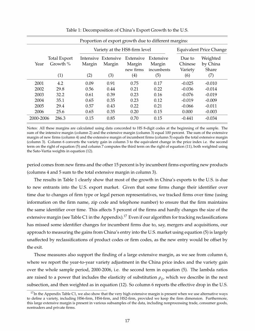
Table 1: Decomposition of China’s Export Growth to the U.S.

Proportion of export growth due to different margins:

Variety at the HS8-firm level Equivalent Price Change

Total Export Intensive Extensive Extensive Extensive Due to WeightedYear Growth % Margin Margin Margin Margin Chinese by China

new firms incumbents Variety Share(1) (2) (3) (4) (5) (6) (7)

2001 4.2 0.09 0.91 0.75 0.17 -0.025 -0.0102002 29.8 0.56 0.44 0.21 0.22 -0.036 -0.0142003 32.2 0.61 0.39 0.23 0.16 -0.076 -0.0192004 35.1 0.65 0.35 0.23 0.12 -0.019 -0.0092005 29.4 0.57 0.43 0.22 0.21 -0.066 -0.0112006 25.6 0.65 0.35 0.20 0.15 0.000 -0.003

2000-2006 286.3 0.15 0.85 0.70 0.15 -0.441 -0.034

Notes: All these margins are calculated using data concorded to HS 8-digit codes at the beginning of the sample. Thesum of the intensive margin (column 2) and the extensive margin (column 3) equal 100 percent. The sum of the extensivemargin of new firms (column 4) and the extensive margin of incumbent firms (column 5) equals the total extensive margin(column 3). Column 6 converts the variety gain in column 3 to the equivalent change in the price index i.e. the secondterm on the right of equation (5) and column 7 computes the third term on the right of equation (11), both weighted usingthe Sato-Vartia weights in equation (12).

period comes from new firms and the other 15 percent is by incumbent firms exporting new products

(columns 4 and 5 sum to the total extensive margin in column 3).

The results in Table 1 clearly show that most of the growth in China’s exports to the U.S. is due

to new entrants into the U.S. export market. Given that some firms change their identifier over

time due to changes of firm type or legal person representatives, we tracked firms over time (using

information on the firm name, zip code and telephone number) to ensure that the firm maintains

the same identifier over time. This affects 5 percent of the firms and hardly changes the size of the

extensive margin (see Table C1 in the Appendix).17 Even if our algorithm for tracking reclassifications

has missed some identifier changes for incumbent firms due to, say, mergers and acquisitions, our

approach to measuring the gains from China’s entry into the U.S. market using equation (5) is largely

unaffected by reclassifications of product codes or firm codes, as the new entry would be offset by

the exit.

Those measures also support the finding of a large extensive margin, as we see from column 6,

where we report the year-to-year variety adjustment in the China price index and the variety gain

over the whole sample period, 2000-2006, i.e. the second term in equation (5). The lambda ratios

are raised to a power that includes the elasticity of substitution ρg, which we describe in the next

subsection, and then weighted as in equation (12). So column 6 reports the effective drop in the U.S.

17In the Appendix Table C1, we also show that the very high extensive margin is present when we use alternative waysto define a variety, including HS6-firm, HS4-firm, and HS2-firm, provided we keep the firm dimension. Furthermore,this large extensive margin is present in various subsamples of the data, including nonprocessing trade, consumer goods,nontraders and private firms.

17

import price index from China due to the new varieties, which amounts to -44 percent over 2000-

2006. Notice that this total change at the bottom of column 6 is not the same as what is obtained

by summing the year-to-year changes in the earlier rows, because the calculation for 2000-2006 is

done on the exports that are “common” to those two years. If there is a new variety exported from

China in 2001, for example, then its growth in exports up to 2006 is attributed to variety growth;

whereas in the earlier rows, only its initial value of exports in 2001 is attributed to variety growth.

This method of using a “long difference” to measure variety growth is consistent with the theory

outlined in section 2, as it allows for increases in the U.S. taste parameter for that Chinese export in

the intervening years, as it penetrates the U.S. market.

To see China’s effect on the overall U.S. manufacturing sector index, we need to adjust the values

of the variety index in column 6 by China’s share in each industry g, which averaged 6 percent

in 2006 and 3 percent in 2000. (These are the weights in the entire U.S. market, and not just the

import shares.) We do this using the Sato-Vartia weights as in the third term in equation (11), before

weighting across industries g as in equation (12). Column 7 shows that the effective price drop due

to variety gain from China is reduced to 3.4 percent — this will be the starting point in our consumer

welfare calculations, in section 5.18

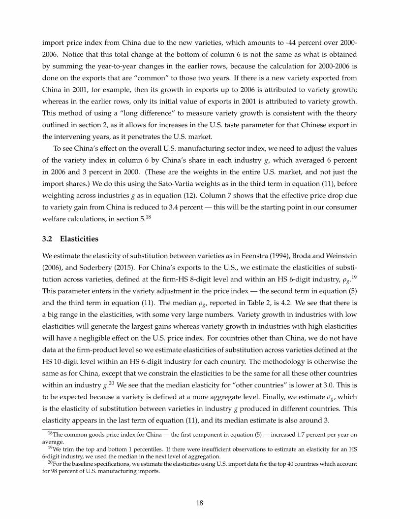
3.2 Elasticities

We estimate the elasticity of substitution between varieties as in Feenstra (1994), Broda and Weinstein

(2006), and Soderbery (2015). For China’s exports to the U.S., we estimate the elasticities of substi-

tution across varieties, defined at the firm-HS 8-digit level and within an HS 6-digit industry, ρg.19

This parameter enters in the variety adjustment in the price index — the second term in equation (5)

and the third term in equation (11). The median ρg, reported in Table 2, is 4.2. We see that there is

a big range in the elasticities, with some very large numbers. Variety growth in industries with low

elasticities will generate the largest gains whereas variety growth in industries with high elasticities

will have a negligible effect on the U.S. price index. For countries other than China, we do not have

data at the firm-product level so we estimate elasticities of substitution across varieties defined at the

HS 10-digit level within an HS 6-digit industry for each country. The methodology is otherwise the

same as for China, except that we constrain the elasticities to be the same for all these other countries

within an industry g.20 We see that the median elasticity for “other countries” is lower at 3.0. This is

to be expected because a variety is defined at a more aggregate level. Finally, we estimate σg, which

is the elasticity of substitution between varieties in industry g produced in different countries. This

elasticity appears in the last term of equation (11), and its median estimate is also around 3.

18The common goods price index for China — the first component in equation (5) — increased 1.7 percent per year onaverage.

19We trim the top and bottom 1 percentiles. If there were insufficient observations to estimate an elasticity for an HS6-digit industry, we used the median in the next level of aggregation.

20For the baseline specifications, we estimate the elasticities using U.S. import data for the top 40 countries which accountfor 98 percent of U.S. manufacturing imports.

18

Table 2: Distribution of Elasticities of Substitution

China ρg Other countries ρg σg

Percentile 5 1.55 1.40 1.51Percentile 25 2.61 2.21 2.21Percentile 50 4.21 2.98 3.08Percentile 75 8.26 5.08 4.31Percentile 95 31.72 28.76 15.83Mean 10.98 9.27 5.42Standard Deviation 32.49 53.70 11.29

Notes:

3.3 Total Factor Productivity

We estimate total factor productivity (TFP) using data on all manufacturing firms in the ASIF sample

for the period 1998 to 2007. We follow Olley and Pakes (1996), by taking account of the simultaneity

between input choices and productivity shocks using firm investment. To estimate the production

coefficients, we use real value added rather than gross output as the dependent variable because

of the large number of processing firms present in China. These processing firms import a large

share of their intermediate inputs and have very low domestic value added (Koopman, Wang, and

Wei (2012)). Real value added is constructed as deflated production less deflated materials. We use

industry level deflators from Brandt, Biesebroeck, and Zhang (2012), where output deflators draw on

“reference prices” from China’s Statistical Yearbooks and the input deflators are constructed using

China’s 2002 national input-output table.21 For the firm’s investment measure, we construct a capital

series using the perpetual inventory method, with real investment calculated as the time difference

in the firm’s capital stock deflated by an annual capital stock deflator. The firm’s real capital stock is

the fixed capital asset at original prices deflated by capital deflators. We begin with the firm’s initial

real capital stock and construct subsequent periods’ real capital stock as K f t = (1− δ)K f ,t−1 + I f t,

where δ is the firm’s actual reported depreciation rate. The production coefficients for each 2-digit

CIC industry, reported in Table C2 in the Appendix, are used to calculate each firm’s log TFP as

follows:22

ln(TFPf t) = ln(VA f t)− βl ln(L f t)− βkln(K f t)

The TFP measures are all normalized relative to the firm’s main 2-digit CIC industry. From Ta-

ble 3, we see that average TFP growth of Chinese exporters has been very high. For the average

exporter in the full sample it has grown 9 percent per year and only slightly more, at 10 percent per

year, in the overlapping sample. For comparison, we also report the average growth in real value

21see http://www.econ.kuleuven.be/public/N07057/CHINA/appendix22For the TFP estimation, we clean the ASIF data on the top and bottom one percentile changes in real value added,

output, materials, and investment rates; and drop any firm with less than 10 employees.

19

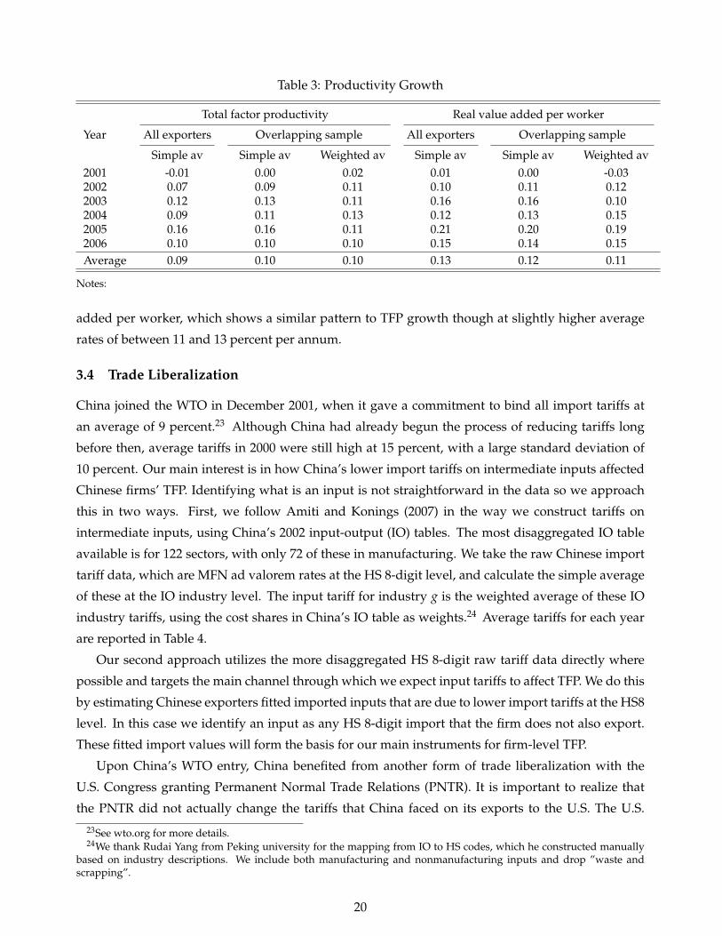
Table 3: Productivity Growth

Total factor productivity Real value added per worker

Year All exporters Overlapping sample All exporters Overlapping sample

Simple av Simple av Weighted av Simple av Simple av Weighted av2001 -0.01 0.00 0.02 0.01 0.00 -0.032002 0.07 0.09 0.11 0.10 0.11 0.122003 0.12 0.13 0.11 0.16 0.16 0.102004 0.09 0.11 0.13 0.12 0.13 0.152005 0.16 0.16 0.11 0.21 0.20 0.192006 0.10 0.10 0.10 0.15 0.14 0.15Average 0.09 0.10 0.10 0.13 0.12 0.11

Notes:

added per worker, which shows a similar pattern to TFP growth though at slightly higher average

rates of between 11 and 13 percent per annum.

3.4 Trade Liberalization

China joined the WTO in December 2001, when it gave a commitment to bind all import tariffs at

an average of 9 percent.23 Although China had already begun the process of reducing tariffs long

before then, average tariffs in 2000 were still high at 15 percent, with a large standard deviation of

10 percent. Our main interest is in how China’s lower import tariffs on intermediate inputs affected

Chinese firms’ TFP. Identifying what is an input is not straightforward in the data so we approach

this in two ways. First, we follow Amiti and Konings (2007) in the way we construct tariffs on

intermediate inputs, using China’s 2002 input-output (IO) tables. The most disaggregated IO table

available is for 122 sectors, with only 72 of these in manufacturing. We take the raw Chinese import

tariff data, which are MFN ad valorem rates at the HS 8-digit level, and calculate the simple average

of these at the IO industry level. The input tariff for industry g is the weighted average of these IO

industry tariffs, using the cost shares in China’s IO table as weights.24 Average tariffs for each year

are reported in Table 4.

Our second approach utilizes the more disaggregated HS 8-digit raw tariff data directly where

possible and targets the main channel through which we expect input tariffs to affect TFP. We do this

by estimating Chinese exporters fitted imported inputs that are due to lower import tariffs at the HS8

level. In this case we identify an input as any HS 8-digit import that the firm does not also export.

These fitted import values will form the basis for our main instruments for firm-level TFP.

Upon China’s WTO entry, China benefited from another form of trade liberalization with the

U.S. Congress granting Permanent Normal Trade Relations (PNTR). It is important to realize that

the PNTR did not actually change the tariffs that China faced on its exports to the U.S. The U.S.

23See wto.org for more details.24We thank Rudai Yang from Peking university for the mapping from IO to HS codes, which he constructed manually

based on industry descriptions. We include both manufacturing and nonmanufacturing inputs and drop ”waste andscrapping”.

20

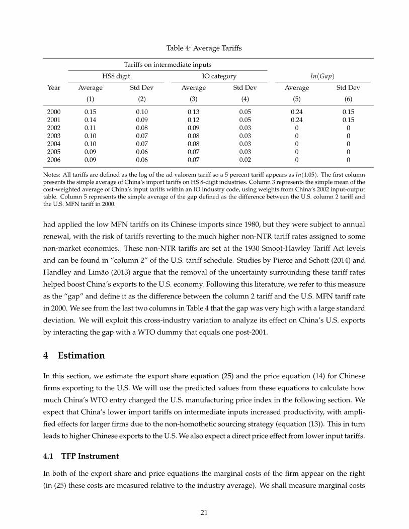
Table 4: Average Tariffs

Tariffs on intermediate inputs

HS8 digit IO category ln(Gap)

Year Average Std Dev Average Std Dev Average Std Dev

(1) (2) (3) (4) (5) (6)

2000 0.15 0.10 0.13 0.05 0.24 0.152001 0.14 0.09 0.12 0.05 0.24 0.152002 0.11 0.08 0.09 0.03 0 02003 0.10 0.07 0.08 0.03 0 02004 0.10 0.07 0.08 0.03 0 02005 0.09 0.06 0.07 0.03 0 02006 0.09 0.06 0.07 0.02 0 0

Notes: All tariffs are defined as the log of the ad valorem tariff so a 5 percent tariff appears as ln(1.05). The first columnpresents the simple average of China’s import tariffs on HS 8-digit industries. Column 3 represents the simple mean of thecost-weighted average of China’s input tariffs within an IO industry code, using weights from China’s 2002 input-outputtable. Column 5 represents the simple average of the gap defined as the difference between the U.S. column 2 tariff andthe U.S. MFN tariff in 2000.

had applied the low MFN tariffs on its Chinese imports since 1980, but they were subject to annual

renewal, with the risk of tariffs reverting to the much higher non-NTR tariff rates assigned to some

non-market economies. These non-NTR tariffs are set at the 1930 Smoot-Hawley Tariff Act levels

and can be found in “column 2” of the U.S. tariff schedule. Studies by Pierce and Schott (2014) and

Handley and Limao (2013) argue that the removal of the uncertainty surrounding these tariff rates

helped boost China’s exports to the U.S. economy. Following this literature, we refer to this measure

as the “gap” and define it as the difference between the column 2 tariff and the U.S. MFN tariff rate

in 2000. We see from the last two columns in Table 4 that the gap was very high with a large standard

deviation. We will exploit this cross-industry variation to analyze its effect on China’s U.S. exports

by interacting the gap with a WTO dummy that equals one post-2001.

4 Estimation

In this section, we estimate the export share equation (25) and the price equation (14) for Chinese

firms exporting to the U.S. We will use the predicted values from these equations to calculate how

much China’s WTO entry changed the U.S. manufacturing price index in the following section. We

expect that China’s lower import tariffs on intermediate inputs increased productivity, with ampli-

fied effects for larger firms due to the non-homothetic sourcing strategy (equation (13)). This in turn

leads to higher Chinese exports to the U.S. We also expect a direct price effect from lower input tariffs.

4.1 TFP Instrument

In both of the export share and price equations the marginal costs of the firm appear on the right

(in (25) these costs are measured relative to the industry average). We shall measure marginal costs

21

inversely by the TFP of each firm, which is influenced by its sourcing strategy. To develop instru-

ments for TFP, we rely on the discussion of the sourcing strategy in Halpern, Koren, and Szeidl (2015)

and Blaum, Lelarge, and Peters (2015). Suppose that the firm uses imported intermediate inputs that

are weakly separable from other domestic inputs. The portion of the production and cost function

devoted to imported inputs is CES, with elasticity of substitution ε > 1. We let c f t ≡ c f (τt, Σ f (τt))

denote that portion of the cost function, which is defined over the prices of inputs n ∈ Σ f (τt) pur-

chased in period t.25 Let Σ f ⊆ Σ f (τ0) ∩ Σ f (τt) denote a non-empty subset of the “common” inputs

purchased in periods 0 and t. Then like the CES indexes in section 2, the index of firm costs between

period t and period 0 is

c f t

c f 0=

∏n∈Σ f

(τnt

τn0

)wnt

( λ f t

λ f 0

) 1ε−1

, (27)

where wnt is the Sato-Vartia weight for input n, and λ f t denotes the expenditure on imported inputs

in the common set Σ f relative to total expenditure on imported inputs in period t. The first term on

the right of (27) is the direct effect of tariffs on costs, or the Sato-Vartia index of input tariffs.26 The

second term is the efficiency gain from expanding the range of inputs, resulting in λ f t < λ f 0 ≤ 1.

This second term corresponds to TFP growth for the firm.

We construct instruments for λ f t by exploiting the highly disaggregated raw tariffs and directly

target the channel through which these operate. We regress Chinese firms’ imports on China’s import

tariffs at the HS 8-digit level — the most disaggregated level available — and use those fitted values

to construct our instruments. More specifically, we estimate the following equation with OLS:

ln(M f nt) = δ f + δt + δ1ln(τint) + δ2Process f × ln(τi

nt) (28)

+ δ3ln(L f )× ln(τint) + δ4 IMR(M f nt) + ε1 f nt.

The dependent variable is the value of firm f imports in HS 8-digit category n, and the Chinese tariffs

τnt are those that apply to those imports. In order to ensure that these imports are actually intermedi-

ate inputs and not final goods, we exclude any import of an HS 8-digit good that the firm exports to

any country in that year. We also interact the tariff with a processing dummy to indicate whether the

input is imported under processing trade, and with the average firm size, measured by employment.

Processing imports already enjoyed duty-free access so a lower tariff on those imports would not

reduce the cost of importing and thus should not have a direct impact on the quantity imported.27

We expect that firms with some portion of ordinary trade to benefit from trade liberalization. We

25As in section 3, we are holding constant the net-of-tariff prices of imported inputs, so these prices are suppressed inthe notation.

26In principle, this first term corresponds to the index of input tariffs that we denoted by Inputτgt. Because Chinesefirms often produce multiple products and we cannot disentangle which of the firm’s imports are used to produce eachof its export goods, we cannot accurately measure the input weight wnt for each input and output. So in practice, weconstruct the index of input tariffs as the industry level g, using the weights from an input-output table.

27We classify a firm as processing if it imports more than 99% of its total intermediate inputs under processing tradeover the sample period.

22

also include year fixed effects and firm fixed effects. Given that the dependent in equation (28) is

undefined for zero imports, we address the potential selection bias by including an inverse mills

ratio IMR(M f nt). The variable is calculated as the ratio of the probability density function to the

cumulative distribution function, from the following import participation equation:

prob(M f nt > 0|X f t = 1) = θg + θt + θ1ln(τint) + θ2Process f × ln(τi

nt) + θ3Process f (29)

+ θ4ln(L f )× ln(τint) + θ5ln(L f ) + θ6Age f t + θ7Foreign f + ε2 f t.

The dependent variable equation equals one if the firm imports an intermediate input in HS 6-digit

category n, and zero otherwise.28 In addition to the variables included in equation (28), we also

include the firm’s age and a foreign ownership indicator to proxy for the firm’s ability to cover the

fixed costs of importing, as in the export participation equation — these will provide our exclusion

restrictions.

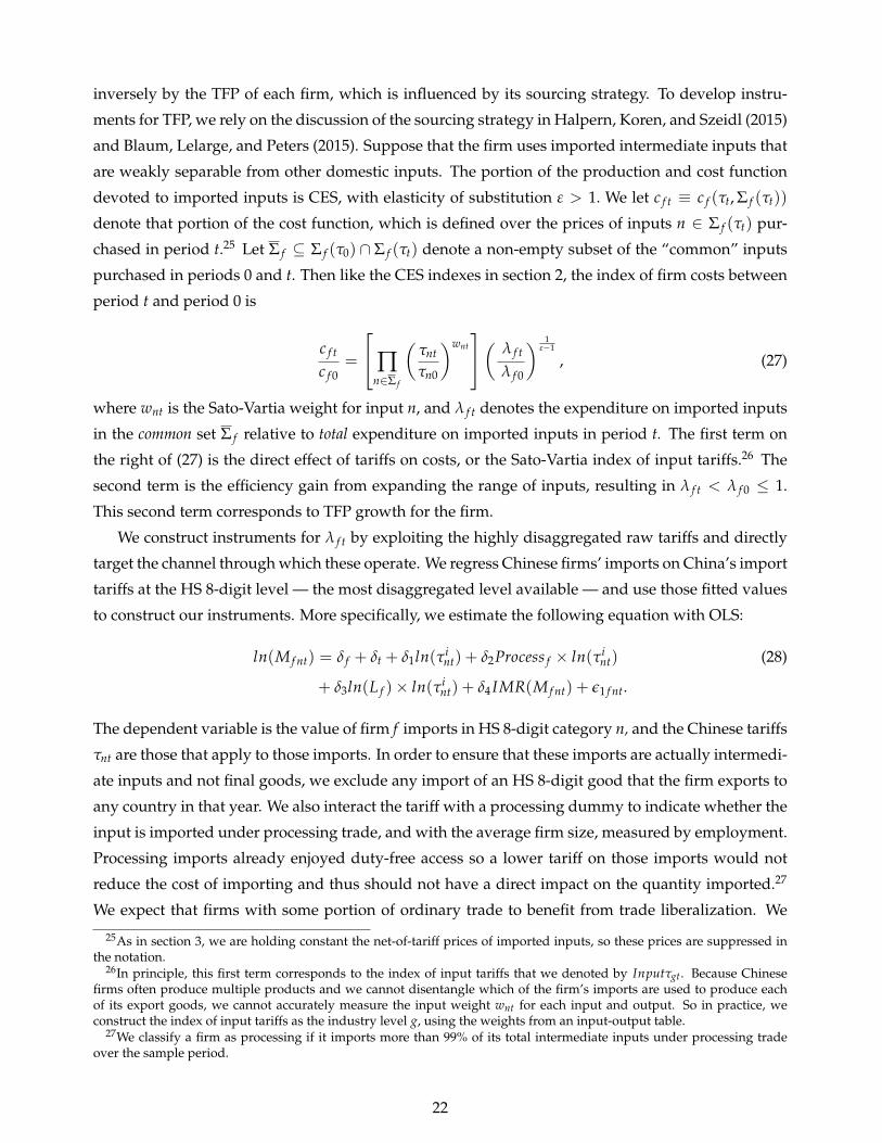
We present the results from estimating the import participation equation in Table 5 and the results

from estimating the import value equation in Table 6.29 In the import participation equation, we also

introduce industry effects to take account that some industries may be high-growth industries due to

factors such as technological progress, however, in a probit we need to be mindful of the incidental

parameters problem induced by too many fixed effects. In Table 5, the first 4 columns are estimated

using probit, with no industry fixed effects in column 1, HS 4-digit industry fixed effects in column

2, and HS 6-digit industry random effects in columns 3 and 4. In the first three columns we interact

tariffs with the firm’s log mean number of workers and in column 4 we use a dummy indicator equal

to one if the firm has more than 1,000 employees. We find that lower tariffs reduce the probability

of importing for processing firms30 and they increase that probability for large nonprocessing firms.

The magnitude of the effect of lower tariffs for large nonprocessing firms is equal to θ1 + θ4× ln(L f ),

which is negative above the threshold of 790 employees — the median number in the sample is 590.

In column 4, we include a “Large” indicator and we see that the coefficient for firms with more than

1,000 workers is equal to -0.25 (summing θ1and θ4), which suggests that large exporting firms are

more likely to import their inputs. We would expect larger firms to be more likely to be able to cover

the fixed costs of importing as they probably have better access to capital markets to finance fixed

costs and working capital. As expected, we find foreign firms are more likely to import their inputs;

however older exporters are less likely to import their inputs. This might appear surprising but we

need to bear in mind that this result is conditional on exporting. We use this equation to construct

the inverse mills ratio for importing, IMR(M f nt), in the import value equation.

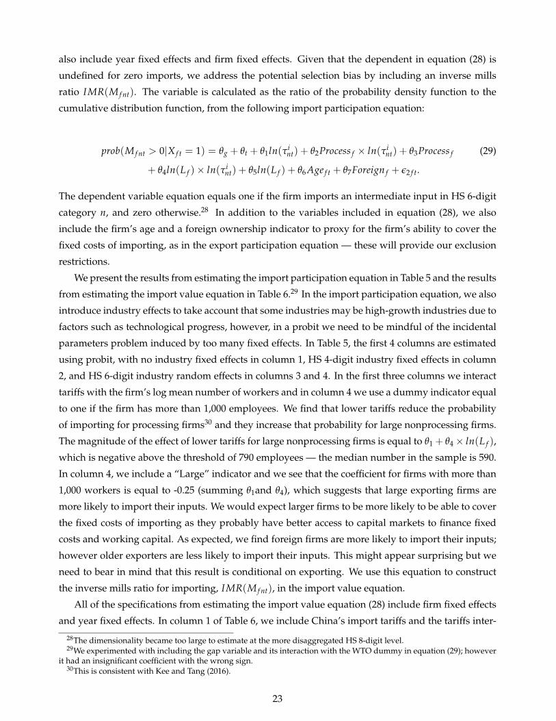
All of the specifications from estimating the import value equation (28) include firm fixed effects

and year fixed effects. In column 1 of Table 6, we include China’s import tariffs and the tariffs inter-

28The dimensionality became too large to estimate at the more disaggregated HS 8-digit level.29We experimented with including the gap variable and its interaction with the WTO dummy in equation (29); however

it had an insignificant coefficient with the wrong sign.30This is consistent with Kee and Tang (2016).

23

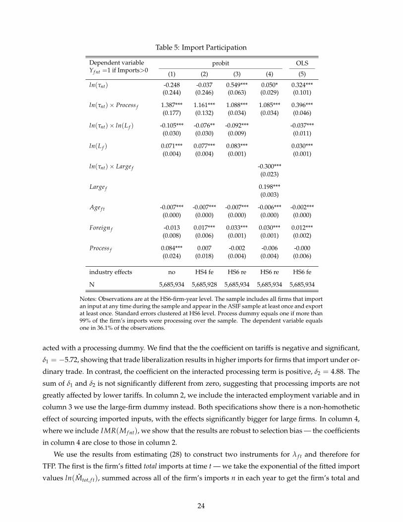
Table 5: Import Participation

Dependent variableYf nt =1 if Imports>0

probit OLS

(1) (2) (3) (4) (5)

ln(τnt) -0.248 -0.037 0.549*** 0.050* 0.324***(0.244) (0.246) (0.063) (0.029) (0.101)

ln(τnt)× Process f 1.387*** 1.161*** 1.088*** 1.085*** 0.396***(0.177) (0.132) (0.034) (0.034) (0.046)

ln(τnt)× ln(L f ) -0.105*** -0.076** -0.092*** -0.037***(0.030) (0.030) (0.009) (0.011)

ln(L f ) 0.071*** 0.077*** 0.083*** 0.030***(0.004) (0.004) (0.001) (0.001)

ln(τnt)× Large f -0.300***(0.023)

Large f 0.198***(0.003)

Age f t -0.007*** -0.007*** -0.007*** -0.006*** -0.002***(0.000) (0.000) (0.000) (0.000) (0.000)

Foreign f -0.013 0.017*** 0.033*** 0.030*** 0.012***(0.008) (0.006) (0.001) (0.001) (0.002)

Process f 0.084*** 0.007 -0.002 -0.006 -0.000(0.024) (0.018) (0.004) (0.004) (0.006)

industry effects no HS4 fe HS6 re HS6 re HS6 fe

N 5,685,934 5,685,928 5,685,934 5,685,934 5,685,934

Notes: Observations are at the HS6-firm-year level. The sample includes all firms that importan input at any time during the sample and appear in the ASIF sample at least once and exportat least once. Standard errors clustered at HS6 level. Process dummy equals one if more than99% of the firm’s imports were processing over the sample. The dependent variable equalsone in 36.1% of the observations.

acted with a processing dummy. We find that the the coefficient on tariffs is negative and significant,

δ1 = −5.72, showing that trade liberalization results in higher imports for firms that import under or-

dinary trade. In contrast, the coefficient on the interacted processing term is positive, δ2 = 4.88. The

sum of δ1 and δ2 is not significantly different from zero, suggesting that processing imports are not

greatly affected by lower tariffs. In column 2, we include the interacted employment variable and in

column 3 we use the large-firm dummy instead. Both specifications show there is a non-homothetic

effect of sourcing imported inputs, with the effects significantly bigger for large firms. In column 4,

where we include IMR(M f nt), we show that the results are robust to selection bias — the coefficients

in column 4 are close to those in column 2.

We use the results from estimating (28) to construct two instruments for λ f t and therefore for

TFP. The first is the firm’s fitted total imports at time t — we take the exponential of the fitted import

values ln(Mtot, f t), summed across all of the firm’s imports n in each year to get the firm’s total and

24

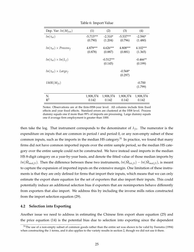
Table 6: Import Value

Dep. Var: ln(M f nt) (1) (2) (3) (4)

ln(τnt) -5.715*** -2.310* -5.537*** -2.590*(0.790) (1.204) (0.796) (1.480)

ln(τnt)× Process f 4.879*** 4.626*** 4.808*** 4.102***(0.878) (0.887) (0.881) (1.365)

ln(τnt)× ln(L f ) -0.512*** -0.466**(0.145) (0.199)

ln(τnt)× Large f -0.568*(0.297)

IMR(M f t) -0.700(1.799)

N 1,908,374 1,908,374 1,908,374 1,908,374R2 0.142 0.142 0.142 0.142

Notes: Observations are at the firm-HS8-year level. All columns include firm fixedeffects and year fixed effects. Standard errors are clustered at the HS8 level. Processdummy equals one if more than 99% of imports are processing. Large dummy equalsone if average firm employment is greater than 1000.

then take the log. That instrument corresponds to the denominator of λ f t. The numerator is the

expenditure on inputs that are common in period t and period 0, or any non-empty subset of these

common inputs, such as the imports in the median HS category.31 In practice, we found that many

firms did not have common imported inputs over the entire sample period, so the median HS cate-

gory over the entire sample could not be constructed. We have instead used imports in the median

HS 8-digit category on a year-by-year basis, and denote the fitted value of those median imports by

ln(Mmed, f t). Then the difference between these two instruments, ln(Mtot, f t)− ln(Mmed, f t), is meant

to capture the expansion of imported inputs on the extensive margin. One limitation of these instru-

ments is that they are only defined for firms that import their inputs, which means that we can only

estimate the export share equation for the set of exporters that also import their inputs. This could

potentially induce an additional selection bias if exporters that are nonimporters behave differently

from exporters that also import. We address this by including the inverse mills ratios constructed

from the import selection equation (29).

4.2 Selection into Exporting

Another issue we need to address in estimating the Chinese firm export share equation (25) and

the price equation (14) is the potential bias due to selection into exporting since the dependent

31The use of a non-empty subset of common goods rather than the entire set was shown to be valid by Feenstra (1994)when constructing the λ terms, and it also applies to the variety results in section 2, though we did not use it there.

25

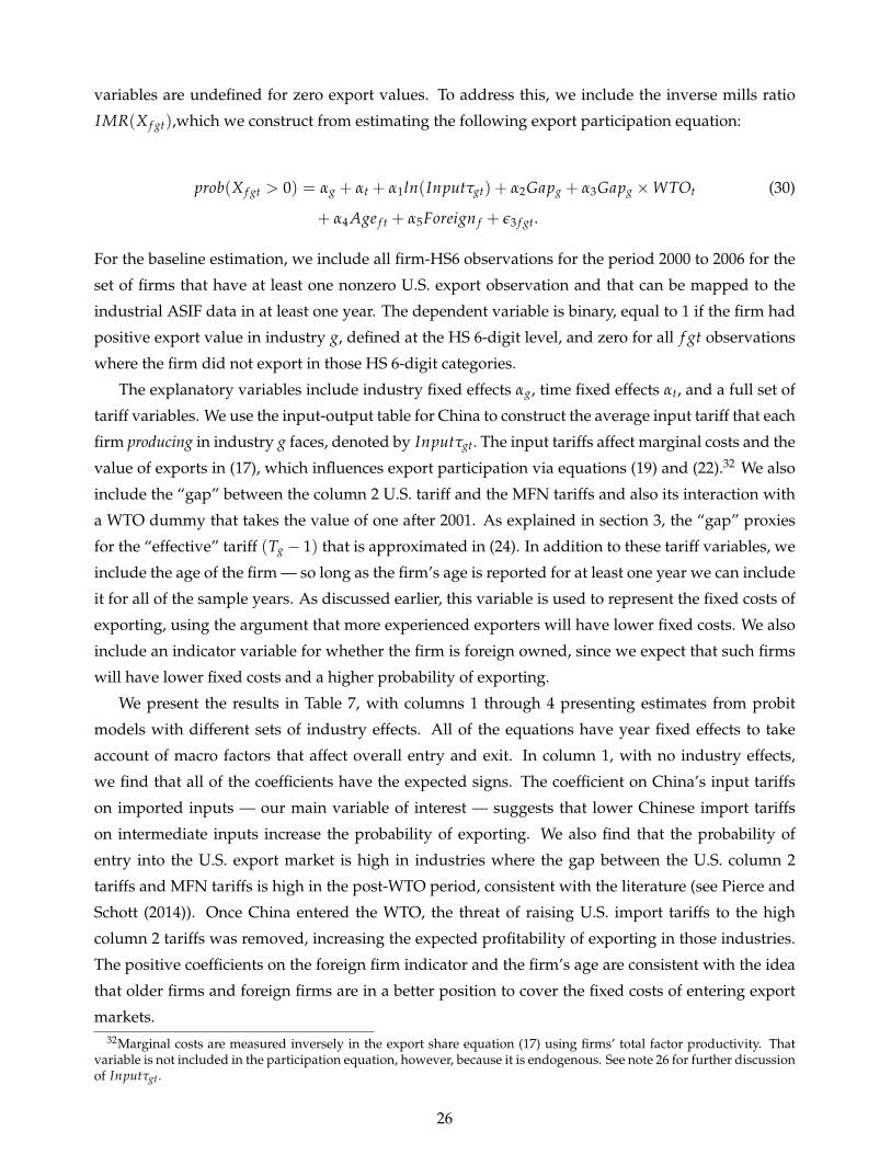
variables are undefined for zero export values. To address this, we include the inverse mills ratio

IMR(X f gt),which we construct from estimating the following export participation equation:

prob(X f gt > 0) = αg + αt + α1ln(Inputτgt) + α2Gapg + α3Gapg ×WTOt (30)

+ α4Age f t + α5Foreign f + ε3 f gt.

For the baseline estimation, we include all firm-HS6 observations for the period 2000 to 2006 for the

set of firms that have at least one nonzero U.S. export observation and that can be mapped to the

industrial ASIF data in at least one year. The dependent variable is binary, equal to 1 if the firm had

positive export value in industry g, defined at the HS 6-digit level, and zero for all f gt observations

where the firm did not export in those HS 6-digit categories.

The explanatory variables include industry fixed effects αg, time fixed effects αt, and a full set of

tariff variables. We use the input-output table for China to construct the average input tariff that each

firm producing in industry g faces, denoted by Inputτgt. The input tariffs affect marginal costs and the

value of exports in (17), which influences export participation via equations (19) and (22).32 We also

include the “gap” between the column 2 U.S. tariff and the MFN tariffs and also its interaction with

a WTO dummy that takes the value of one after 2001. As explained in section 3, the “gap” proxies

for the “effective” tariff (Tg − 1) that is approximated in (24). In addition to these tariff variables, we

include the age of the firm — so long as the firm’s age is reported for at least one year we can include

it for all of the sample years. As discussed earlier, this variable is used to represent the fixed costs of

exporting, using the argument that more experienced exporters will have lower fixed costs. We also

include an indicator variable for whether the firm is foreign owned, since we expect that such firms

will have lower fixed costs and a higher probability of exporting.

We present the results in Table 7, with columns 1 through 4 presenting estimates from probit

models with different sets of industry effects. All of the equations have year fixed effects to take

account of macro factors that affect overall entry and exit. In column 1, with no industry effects,

we find that all of the coefficients have the expected signs. The coefficient on China’s input tariffs

on imported inputs — our main variable of interest — suggests that lower Chinese import tariffs

on intermediate inputs increase the probability of exporting. We also find that the probability of

entry into the U.S. export market is high in industries where the gap between the U.S. column 2

tariffs and MFN tariffs is high in the post-WTO period, consistent with the literature (see Pierce and

Schott (2014)). Once China entered the WTO, the threat of raising U.S. import tariffs to the high

column 2 tariffs was removed, increasing the expected profitability of exporting in those industries.

The positive coefficients on the foreign firm indicator and the firm’s age are consistent with the idea

that older firms and foreign firms are in a better position to cover the fixed costs of entering export

markets.32Marginal costs are measured inversely in the export share equation (17) using firms’ total factor productivity. That

variable is not included in the participation equation, however, because it is endogenous. See note 26 for further discussionof Inputτgt.

26

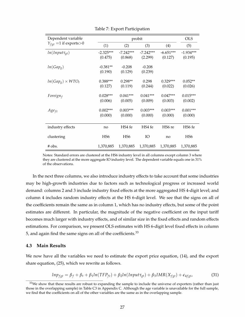
Table 7: Export Participation

Dependent variableYf gt =1 if exports>0

probit OLS

(1) (2) (3) (4) (5)

ln(Inputτgt) -2.325*** -7.242*** -7.242*** -6.651*** -1.934***(0.475) (0.868) (2.299) (0.127) (0.195)

ln(Gapg) -0.381** -0.208 -0.208(0.190) (0.129) (0.239)

ln(Gapg)×WTOt 0.388*** 0.298** 0.298 0.329*** 0.052**(0.127) (0.119) (0.244) (0.022) (0.026)

Foreign f 0.028*** 0.041*** 0.041*** 0.047*** 0.015***(0.006) (0.005) (0.009) (0.003) (0.002)

Age f t 0.002*** 0.003*** 0.003*** 0.003*** 0.001***(0.000) (0.000) (0.000) (0.000) (0.000)

industry effects no HS4 fe HS4 fe HS6 re HS6 fe

clustering HS6 HS6 IO no HS6

# obs. 1,370,885 1,370,885 1,370,885 1,370,885 1,370,885

Notes: Standard errors are clustered at the HS6 industry level in all columns except column 3 wherethey are clustered at the more aggregate IO industry level. The dependent variable equals one in 31%of the observations.

In the next three columns, we also introduce industry effects to take account that some industries

may be high-growth industries due to factors such as technological progress or increased world

demand: columns 2 and 3 include industry fixed effects at the more aggregated HS 4-digit level; and

column 4 includes random industry effects at the HS 6-digit level. We see that the signs on all of

the coefficients remain the same as in column 1, which has no industry effects, but some of the point

estimates are different. In particular, the magnitude of the negative coefficient on the input tariff

becomes much larger with industry effects, and of similar size in the fixed effects and random effects

estimations. For comparison, we present OLS estimates with HS 6-digit level fixed effects in column

5, and again find the same signs on all of the coefficients.33

4.3 Main Results

We now have all the variables we need to estimate the export price equation, (14), and the export

share equation, (25), which we rewrite as follows.

lnp f gt = β f + βt + β1ln(TFPf t) + β2ln(Inputτgt) + β3 IMR(X f gt) + ε4 f gt, (31)

33We show that these results are robust to expanding the sample to include the universe of exporters (rather than justthose in the overlapping sample) in Table C3 in Appendix C. Although the age variable is unavailable for the full sample,we find that the coefficients on all of the other variables are the same as in the overlapping sample.

27

and

ln(X f gt/Xgt) = γ f + γt + γ1ln(TFPf t) + γ2ln(Ngt) + γ3 IMR(X f gt) + ε5 f gt. (32)

The dependent variable in the pricing equation is the log unit value, inclusive of freight, insur-

ance, and duties.34 The pricing equation (31) includes the average tariff on inputs at the industry

level, Inputτgt, but that variable does not appear in the export share equation (32) because it is com-

mon to all Chinese exporters in the industry (and hence cancels out). Further, because the dependent

variable is a share variable, the TFP on the right side of equation (32) is TFP relative to the industry

average. If all firms had equal productivity, they would set the same prices and shares, so the export

share for every firm would be 1/N, which is why the export share equation includes the log number

of Chinese exporters, ln(Ngt), as shown in (25), with a coefficient of -1. Then from the relative TFP

term, firms with higher than average productivity will have higher than average export shares. Both

the TFP and the N terms are treated as endogenous. We instrument for TFP using the two instru-

ments we constructed from the fitted import values above. We instrument for the number of Chinese

firms exporting to the U.S. in each industry with the number of Chinese firms exporting to EU coun-

tries. We also experiment with an alternative instrument constructed from the predicted number of

exporters obtained by summing the predicted probability of exporting from the participation equa-

tion (30).

Our model implies the coefficients γ1 = β1(1− ρg), β2 = 1, γ2 = −1. Given that we do not allow

the coefficients to differ across industries g, a better way to capture this cross-equation restriction is

with γ1 = β1(1− ρmed), using a median estimate ρmed. We will not find coefficients satisfying these

cross-equation constraints, however, and a model-based reason for this finding is that the error terms

in both equations include the unobserved quality of the export product. To see how unobserved

quality can influence the coefficient estimates, notice that from (31) the error term in the pricing

equation, ε4 f gt, includes log quality, which we now denote by lnz f gt instead of lnzijg (ϕ). Suppose that

quality is linearly related to TFP according to lnz f gt = ζln(TFPf t) + u f gt, for an error term u f gt that

is uncorrelated with the other variables on the right of (31) or (32). In the price regression, then,

the coefficient estimates on TFP in (31) becomes the biased estimate β1 = β1 + ζ. In the export

share equation (32), log quality enters the error term with the coefficient ρg − 1, as shown by (25).

Replacing this with a median estimate ρmed − 1, the coefficient estimates on TFP in (32) becomes

γ1 = γ1 + (ρmed − 1)ζ, which is alternatively written as γ1 = (ρmed − 1)(ζ − β1) using the cross-

equation restriction γ1 = β1(1 − ρmed). Using these two biased estimates, we therefore solve for

the unbiased estimates β1 = 0.5[β1 − γ1/(ρmed − 1)] and γ1 = 0.5[(1− ρmed)β1 + γ1], as we shall

compute.35

The results from estimating equation (31) and (32) are summarized in Table (8) and Table (9). All

34The results are unchanged for unit values that exclude duties because the U.S. MFN import tariffs are very low andhave hardly changed over the sample period. For this reason, the MFN tariff is not included on the right of (31).

35Adjusting the estimated coefficients in this way did not affect our conclusions in the final decomposition below.

28

of the equations include firm fixed effects and year fixed effects.36 In column 1, we present the re-

sults using OLS as a benchmark for all exporters in the overlapping sample. The coefficient on the log

number of exporters in an HS6 industry is negative one as indicated by the theory. Our main interest

is in the coefficient on the log TFP, constructed at the firm level. As expected, we find that firms with

higher TFP export more. However, we are concerned that the magnitude is biased due to the issues

we raised above. To address endogeneity, we instrument for both ln(TFPf gt) and ln(Ngt) in all of

the the subsequent columns with the following instrument set: the fitted import values from equa-

tion (28) for the total and median imported input expenditure; the log gap interacted with the WTO

dummy equal to 1 post-2001; and the number of Chinese firms exporting to the EU, which pass the

weak instrument test and the overidentification tests. With the instrumental variables estimation, we

see that the coefficient on TFP jumps to 1.2 in column 2 — much larger than the OLS coefficient of 0.1

in column 1. In column 3, we control for potential selection bias by including the IMR(X) constructed

from the export participation equation, since the dependent variable is undefined for zero export

shares; and we include the IMR(M) to take account of the fact that our fitted import instruments are

undefined for nonimporters. The coefficients on both the IMR’s turn out to be insignificant and leave

the TFP coefficient unchanged.

Another potential issue is that the dependent variable is at the firm-industry level whereas the

TFP is at the firm level. Ideally, we would have a measure of TFP for each product that a firm

produces but that is not possible. This could be problematic because our average firm-level TFP

measure is unlikely to be representative of the smaller export share products, which would result in

a downward bias. So in column 4, we exclude any observation for which the Chinese firm’s exports

within its total U.S. exports that year were less than 5 percent. We see that this makes an enormous

difference with the coefficient on TFP more than tripling.37 We also experimented with alternative

cutoffs, with all giving similar results, and in column 4 we report the case where we only include

the firm’s largest value HS 6-digit U.S. export, and the TFP coefficient is 4.5. The coefficient on the

log number of firms remains close to -1 in all of the specifications. These magnitudes are consistent

with that implied by equation (25), where the coefficient on log TFP is equal to ρg − 1; recall that the

median ρg we estimated is equal to 4.2.

Turning to the first-stage results, reported in the bottom panel of Table 8, the coefficients on

the instruments have the expected signs, with higher total imports boosting TFP. However, the gap

variable is only significant in the column 3 specification which has the full sample of firms. It becomes

insignificant as soon as we exclude the smallest export shares (see the first stage results for columns

4 and 5 specifications). We also checked whether it might be significant in the second stage equation

(column 6) and there we find it is insignificant and of the wrong sign. These results suggest that

elimination of the gap did not result in a higher intensive margin. However, we do find there were

36Because firms produce multiple products and sometimes switch product categories, the full set of firm fixed effectsdoes not quite span the space of industry fixed effects. So we also include industry fixed effects αg when estimating thisequation, though most of these fixed effects are dropped due to multicollinearity.

37Similarly, if we reestimate the OLS column 1 for the limited sample we find that its coefficient triples.

29

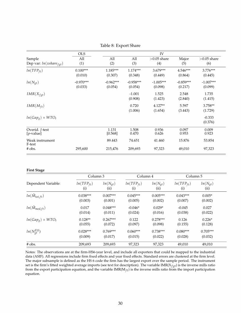
Table 8: Export Share

OLS IVSample All All All >0.05 share Major >0.05 shareDep var: ln(xshare f gt) (1) (2) (3) (4) (5) (6)

ln(TFPf t) 0.100*** 1.185*** 1.174*** 3.679*** 4.546*** 3.776***(0.010) (0.307) (0.348) (0.449) (0.864) (0.445)

ln(Ngt) -0.970*** -0.962*** -0.958*** -1.005*** -0.859*** -1.007***(0.033) (0.054) (0.054) (0.098) (0.217) (0.099)

IMR(X f gt) -1.001 1.525 2.548 1.735(0.908) (1.423) (2.840) (1.415)

IMR(M f t) 0.720 4.127** 5.597 3.758**(1.006) (1.654) (3.443) (1.729)

ln(Gapg)×WTOt -0.333(0.376)

Overid. J-test 1.131 1.508 0.936 0.097 0.009[p-value] [0.568] 0.470 0.626 0.953 0.923

Weak instrument 89.443 74.651 41.460 15.876 53.854F-test# obs. 295,600 215,476 209,693 97,323 49,010 97,323

First Stage

Column 3 Column 4 Column 5

Dependent Variable: ln(TFPf t) ln(Ngt) ln(TFPf t) ln(Ngt) ln(TFPf t) ln(Ngt)(i) (ii) (i) (ii) (i) (ii)

ln(Mtot, f t) 0.038*** 0.007*** 0.045*** 0.005*** 0.043*** 0.005*(0.003) (0.001) (0.005) (0.002) (0.007) (0.002)

ln(Mmed, f t) 0.017 0.048*** -0.046* 0.029* -0.045 0.027(0.014) (0.011) (0.024) (0.016) (0.038) (0.022)

ln(Gapg)×WTOt 0.128** 0.267*** 0.122 0.278*** 0.126 0.226*(0.055) (0.072) (0.097) (0.098) (0.155) (0.128)

ln(NEUgt ) 0.028*** 0.769*** 0.060*** 0.738*** 0.080*** 0.705***

(0.009) (0.017) (0.015) (0.022) (0.028) (0.032)

# obs. 209,693 209,693 97,323 97,323 49,010 49,010

Notes: The observations are at the firm-HS6-year level, and include all exporters that could be mapped to the industrialdata (ASIF). All regressions include firm fixed effects and year fixed effects. Standard errors are clustered at the firm level.The major subsample is defined as the HS 6 code the firm has the largest export over the sample period. The instrumentset is the firm’s fitted weighted average imports (see text for description). The variable IMR(X f gt) is the inverse mills ratiofrom the export participation equation, and the variable IMR(M f t) is the inverse mills ratio from the import participationequation.

30

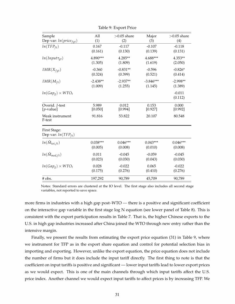
Table 9: Export Price

Sample All >0.05 share Major >0.05 shareDep var: ln(price f gt) (1) (2) (3) (4)ln(TFPf t) 0.167 -0.117 -0.107 -0.118

(0.161) (0.130) (0.139) (0.131)

ln(Inputτgt) 4.890*** 4.285** 4.688*** 4.353**(1.305) (1.809) (1.619) (2.050)

IMR(X f gt) -0.360 -0.831** -0.596 -0.826*(0.324) (0.399) (0.521) (0.414)

IMR(M f t) -2.438** -2.937** -3.846*** -2.998**(1.009) (1.255) (1.145) (1.389)

ln(Gapg)×WTOt -0.011(0.112)

Overid. J-test 5.989 0.012 0.153 0.000[p-value] [0.050] [0.994] [0.927] [0.992]

Weak instrument 91.816 53.822 20.107 80.548F-test

First Stage:Dep var: ln(TFPf t)

ln(Mtot, f t) 0.038*** 0.046*** 0.043*** 0.046***(0.005) (0.008) (0.010) (0.008)

ln(Mmed, f t) 0.011 -0.045 -0.059 -0.045(0.023) (0.030) (0.043) (0.030)

ln(Gapg)×WTOt 0.028 -0.022 0.065 -0.022(0.175) (0.276) (0.410) (0.276)

# obs. 197,292 90,789 45,709 90,789

Notes: Standard errors are clustered at the IO level. The first stage also includes all second stagevariables, not reported to save space.

more firms in industries with a high gap post–WTO — there is a positive and significant coefficient

on the interactive gap variable in the first stage log N equation (see lower panel of Table 8). This is

consistent with the export participation results in Table 7. That is, the higher Chinese exports to the

U.S. in high gap industries increased after China joined the WTO through new entry rather than the

intensive margin.

Finally, we present the results from estimating the export price equation (31) in Table 9, where

we instrument for TFP as in the export share equation and control for potential selection bias in

importing and exporting. However, unlike the export equation, the price equation does not include

the number of firms but it does include the input tariff directly. The first thing to note is that the

coefficient on input tariffs is positive and significant — lower input tariffs lead to lower export prices

as we would expect. This is one of the main channels through which input tariffs affect the U.S.

price index. Another channel we would expect input tariffs to affect prices is by increasing TFP. We

31

find this channel is more difficult to detect in the price regression. It is insignificant in all of the

specifications, but does switch from being positive in the full sample in column 1 to the expected

negative sign as soon as we omit firms’ tiny export shares. We suspect that this is due to the quality

bias and we can correct for this as described above. In the first stage results in the lower panel of

Table (9) we see that the total fitted import values have a positive effect on TFP but the gap variable is

again insignificant (and close to zero) and switches signs across specifications. We further experiment

with including the gap term in the second stage equation in the upper panel of column 4 and find

it is insignificant and close to zero. These results suggest that the gap variable does not affect prices

consistent with our theory, as prices are chosen after the tariff is known.

To summarize this section, the results show that lower Chinese input tariffs increase Chinese

firms’ imports of intermediate inputs, both on the intensive and extensive margins, and thus increase

their TFP. This, in turn, increases their export shares relative to the average firm, as well as increasing

the probability of entry into the U.S. market. Lower input tariffs also lower Chinese firms export

prices in the U.S. market. The effect from PNTR is more limited. There is no direct effect on export

prices nor on export shares — the only effect we detected was through new entry into exporting. We

now turn to evaluate how these effects feed into the U.S. price index.

5 The Impact of China’s WTO Entry

With our regression results in hand, we turn to estimating the impact of China’s WTO entry on U.S.

consumer welfare (treating U.S. importing households and firms as “consumers”). Our starting point

is equation (11). We call the first term on the right of (11) the U.S. import price index of common Chi-

nese goods, or ChinaPg; the second term is the common goods price index from all other countries,

including the U.S.; the third term is the Chinese variety component of imports, or ChinaVg; and the

fourth term is the variety component from other countries (including the U.S.), or OtherVg. We shall

regress each of these terms on two instruments that we construct, based on China’s entry to the WTO.

The first China WTO instrument is the change in Chinese exporter prices predicted from equation

(31). Letting the year 2000 represent the base period 0, we predict prices in 2006 relative to 2000. Then

we construct the instrument as follows:

ˆChinaPg ≡ lnPgt

Pg0= ln

∏f h∈Ωg

(p f ht

p f h0

)w f ht

, (33)

where Ωg = Ωgt ∩ Ωg0 is the set of varieties (at the firm-product level, f h) that were exported in

industry g during both year 2006 and 2000, and w f ht are the Sato-Vartia weights over these varieties.

Note that this instrument uses only the predicted export prices from Chinese firms, and does not

include any prices from other exporters to the U.S. nor prices of U.S. domestic producers.

The second WTO instrument uses fitted values from the China firm export share equation (32).

For convenience let x f gt ≡ X f gt/Xgt denote the exporter share on the left of (32), with predicted

32

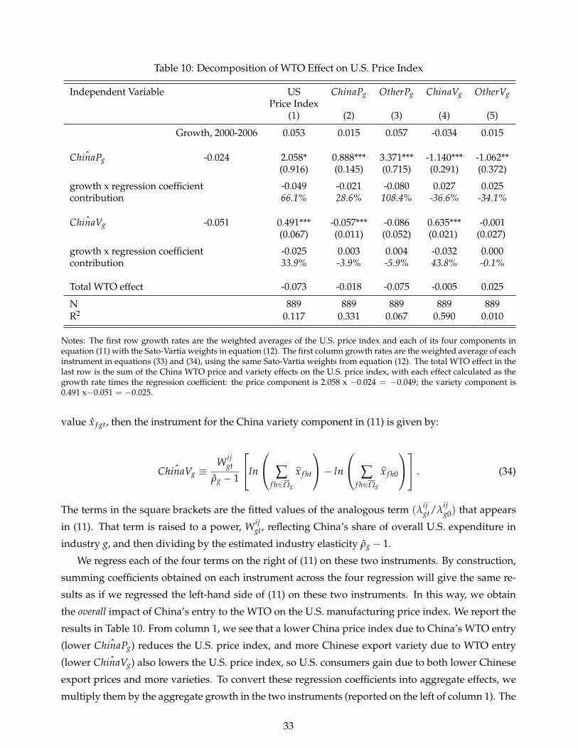
Table 10: Decomposition of WTO Effect on U.S. Price Index

Independent Variable US ChinaPg OtherPg ChinaVg OtherVgPrice Index

(1) (2) (3) (4) (5)

Growth, 2000-2006 0.053 0.015 0.057 -0.034 0.015

ˆChinaPg -0.024 2.058* 0.888*** 3.371*** -1.140*** -1.062**(0.916) (0.145) (0.715) (0.291) (0.372)

growth x regression coefficient -0.049 -0.021 -0.080 0.027 0.025contribution 66.1% 28.6% 108.4% -36.6% -34.1%

ˆChinaVg -0.051 0.491*** -0.057*** -0.086 0.635*** -0.001(0.067) (0.011) (0.052) (0.021) (0.027)

growth x regression coefficient -0.025 0.003 0.004 -0.032 0.000contribution 33.9% -3.9% -5.9% 43.8% -0.1%

Total WTO effect -0.073 -0.018 -0.075 -0.005 0.025

N 889 889 889 889 889R2 0.117 0.331 0.067 0.590 0.010

Notes: The first row growth rates are the weighted averages of the U.S. price index and each of its four components inequation (11) with the Sato-Vartia weights in equation (12). The first column growth rates are the weighted average of eachinstrument in equations (33) and (34), using the same Sato-Vartia weights from equation (12). The total WTO effect in thelast row is the sum of the China WTO price and variety effects on the U.S. price index, with each effect calculated as thegrowth rate times the regression coefficient: the price component is 2.058 x −0.024 = −0.049; the variety component is0.491 x−0.051 = −0.025.

value x f gt, then the instrument for the China variety component in (11) is given by:

ˆChinaVg ≡W ij

gt

ρg − 1

ln

∑f h∈Ωg

x f ht

− ln

∑f h∈Ωg

x f h0

. (34)

The terms in the square brackets are the fitted values of the analogous term (λijgt/λ

ijg0) that appears

in (11). That term is raised to a power, W ijgt, reflecting China’s share of overall U.S. expenditure in

industry g, and then dividing by the estimated industry elasticity ρg − 1.

We regress each of the four terms on the right of (11) on these two instruments. By construction,

summing coefficients obtained on each instrument across the four regression will give the same re-

sults as if we regressed the left-hand side of (11) on these two instruments. In this way, we obtain

the overall impact of China’s entry to the WTO on the U.S. manufacturing price index. We report the

results in Table 10. From column 1, we see that a lower China price index due to China’s WTO entry

(lower ˆChinaPg) reduces the U.S. price index, and more Chinese export variety due to WTO entry

(lower ˆChinaVg) also lowers the U.S. price index, so U.S. consumers gain due to both lower Chinese

export prices and more varieties. To convert these regression coefficients into aggregate effects, we

multiply them by the aggregate growth in the two instruments (reported on the left of column 1). The

33

sum of these two values indicates that the total WTO effect on the U.S. price index is -0.073 i.e. the

U.S. manufacturing price index was 7.3 percent lower in 2006 relative to 2000 due to China joining

the WTO.

Now, let’s consider how each of these instruments affected each of the components of the U.S.

price index. The largest effect is coming through ˆChinaPg. As expected, the lower China price in-

strument lowers the China common goods price index (column 2). Interestingly, it also has a very

big effect on competitor prices in column 3, which may reflect exit of inefficient competitor firms,

lower marginal costs or lower markups. Further, a lower ˆChinaPg causes exit of some competitor

Chinese firms (column 4) and other competitor firms (column 5). Turning to the variety instrument

in the lower half of the table, we see that increased Chinese variety due to WTO increases the China

variety component in column 4, though this is somewhat muted with a coefficient of 0.6, and it has

no effect on other competitors (column 5). We also find that a lower ˆChinaVg leads to higher Chinese

prices in column 2 and competitor prices in column 3, though these are both very small effects, and

we suspect that the negative coefficients are due to a quality bias.

The decomposition in Table 10 shows that two-thirds of the China WTO effect on the U.S. price

index comes through China’s price instrument. The finding that most of the gains come through a

lower ˆChinaPg rather than a lower ˆChinaVg is somewhat surprising given the large extensive margin

of exporting we documented above. In fact, most of the consumer gain comes from China’s impact

on competitor prices. Given that the gap does not affect ˆChinaPg at all, since it had no effect on

Chinese export prices, as shown in Table 9, we can conclude that at least two-thirds of the WTO

effect was indeed due to lower Chinese tariffs on intermediate inputs.

6 Conclusion

In this paper, we quantify the effect of China’s WTO entry on U.S. consumers. We construct U.S.

manufacturing price indexes by combining highly disaggregated Chinese firm-product data for the

period 2000 to 2006, with U.S. import data from other countries and U.S. domestic sales. To take

account of new product varieties, we construct exact CES price indexes, which comprise both a price

and variety component. We find that China’s WTO entry reduced the U.S. manufactured goods price

index by 7.3 percent. Two thirds of this effect arose through the conventional price index compo-

nent, despite there being a huge extensive margin of exporting. Importantly, our analysis explicitly

takes account of China’s trade shock on competitor prices and entry. Our results indicate that lower

Chinese export prices due to WTO entry reduced both the China price index and the prices of com-

petitor firms in the U.S., which also led to exit of Chinese competitors and other competitors in the

U.S. These effects could be due to less efficient firms exiting the U.S. market, lower marginal costs or

lower markups.

Our paper is the first to show that the key mechanism underlying the China WTO effect on U.S.

price indexes is China lowering its own import tariffs on intermediate inputs. Indeed, we find that

34

lower Chinese tariffs on its intermediate inputs increased its import values and varieties, which in

turn boosted Chinese firms productivity. This higher productivity meant that new firms could enter

the U.S. market and increase their market shares. In addition, lower input tariffs have a direct effect

on Chinese export prices. We also allow for China’s access to PNTR under WTO to affect Chinese

exports — a channel that has received a lot of attention — and consistent with the literature we show

that PNTR does result in higher entry into exporting. However, we find no effect of PNTR on Chinese

firms TFP, export prices, or the intensive margin of exporting. As such, most of the WTO effect on

U.S. price indexes comes through China’s lower input tariffs; accounting for at least two thirds of the

overall effect. These gains are additional to the standard gains from trade that arise from reducing

iceberg trade costs and in addition to the gains from reducing uncertainty.

35

References

ACEMOGLU, D., D. AUTOR, D. DORN, G. H. HANSON, AND B. PRICE (2014): “Import Competition

and the Great U.S. Employment Sag of the 2000s,” NBER Working Papers 20395.

AMITI, M., O. ITSKHOKI, AND J. KONINGS (2014): “Importers, Exporters, and Exchange Rate Dis-

connect,” American Economic Review, 104(7), 1942–78.

AMITI, M., AND J. KONINGS (2007): “Trade Liberalization, Intermediate Inputs, and Productivity:

Evidence from Indonesia,” American Economic Review, 97(5), 1611–1638.

ANTRAS, P., T. C. FORT, AND F. TINTELNOT (2014): “The Margins of Global Sourcing: Theory and

Evidence from U.S. Firms,” Working Paper 154856, Harvard University OpenScholar.

ARKOLAKIS, C., A. COSTINOT, AND A. RODRIGUEZ-CLARE (2012): “New Trade Models, Same Old

Gains?,” American Economic Review, 102(1), 94–130.

AUTOR, D. H., D. DORN, AND G. H. HANSON (2013): “The China Syndrome: Local Labor Market

Effects of Import Competition in the United States,” American Economic Review, 103(6), 2121–68.

BAS, M. (2012): “Input-trade liberalization and firm export decisions: Evidence from Argentina,”

Journal of Development Economics, 97(2), 481–493.

BAS, M., AND V. STRAUSS-KAHN (2014): “Does importing more inputs raise exports? Firm-level

evidence from France,” Review of World Economics (Weltwirtschaftliches Archiv), 150(2), 241–275.

BLAUM, J., C. LELARGE, AND M. PETERS (2015): “The Gains From Input Trade in Firm-Based Models

of Importing,” .

BLOOM, N., M. DRACA, AND J. VAN REENEN (2011): “Trade induced technical change? The impact

of Chinese imports on innovation, IT and productivity,” CEPR Discussion Papers 8236.

BRANDT, L., J. V. BIESEBROECK, AND Y. ZHANG (2012): “Creative Accountng or creative destruction?

Firm-level productivity growth in Chinese manufacturing,” Journal of Development Economics, 97,

339–351.

BRANDT, L., J. VAN BIESEBROECK, L. WANG, AND Y. ZHANG (2012): “WTO Accession and Perfor-

mance of Chinese Manufacturing Firms,” CEPR Discussion Papers 9166.

BRODA, C., AND D. E. WEINSTEIN (2006): “Globalization and the Gains from Variety,” The Quarterly

Journal of Economics, 121(2), 541–585.

CALIENDO, L., M. DVORKIN, AND F. PARRO (2015): “The Impact of Trade on Labor Market Dynam-

ics,” NBER Working Paper 21149.

36

CALIENDO, L., R. C. FEENSTRA, J. ROMALIS, AND A. M. TAYLOR (2015): “Tariff Reductions, Entry

and Welfare: Theory and Evidence from the last Two Decades,” NBER Working Paper 21768.

COSTINOT, A., AND A. RODRIGUEZ-CLARE (2014): “Trade Theory with Numbers: Quantifying the

Consequences of Globalization,” in Handbook of International Economics, volume 4, edited by Gita

Gopinath, Elhanan Helpman, and Kenneth Rogoff, pp. 197–262. Elsevier.

DI GIOVANNI, J., A. A. LEVCHENKO, AND J. ZHANG (2014): “The Global Welfare Impact of China:

Trade Integration and Technological Change,” American Economic Journal: Macroeconomics, 6(3),

153–83.

FAN, H., Y. A. LI, AND S. R. YEAPLE (2014): “Trade Liberalization, Quality, and Export Prices,”

NBER Working Papers 20323.

FEENSTRA, R. C. (1994): “New Product Varieties and the Measurement of International Prices,”

American Economic Review, 84(1), 157–77.

FEENSTRA, R. C., AND D. E. WEINSTEIN (2015): “Globalization, Markups and U.S. Welfare,” Journal

of Political Economy, forthcoming.

FENG, L., Z. LI, AND D. L. SWENSON (2012): “The Connection between Imported Intermediate

Inputs and Exports: Evidence from Chinese Firms,” NBER Working Papers 18260.

(2015): “Trade Policy Uncertainty and Exports: Evidence from China’s WTO Accession,” .

GOLDBERG, P. K., A. K. KHANDELWAL, N. PAVCNIK, AND P. TOPALOVA (2010): “Imported In-

termediate Inputs and Domestic Product Growth: Evidence from India,” The Quarterly Journal of

Economics, 125(4), 1727–1767.

GOPINATH, G., AND B. NEIMAN (2014): “Trade Adjustment and Productivity in Large Crises,” Amer-

ican Economic Review, 104(3), 793–831.

HALPERN, L., M. KOREN, AND A. SZEIDL (2015): “Imported Inputs and Productivity,” American

Economic Review, 105(12), 3660–3703.

HANDLEY, K., AND N. LIMAO (2013): “Policy Uncertainty, Trade and Welfare: Theory and Evidence

for China and the U.S,” CEPR Discussion Papers 9615, C.E.P.R. Discussion Papers.

HOPENHAYN, H. (1992): “Entry, Exit, and Firm Dynamics in Long Run Equilibrium,” Econometrica,

60(5), 1127–1150.

HSIEH, C.-T., AND R. OSSA (2011): “A Global View of Productivity Growth in China,” Global COE

Hi-Stat Discussion Paper Series gd10-166, Institute of Economic Research, Hitotsubashi University.

IACOVONE, L., F. RAUCH, AND L. A. WINTERS (2013): “Trade as an engine of creative destruction:

Mexican experience with Chinese competition,” Journal of International Economics, 89(2), 379–392.

37

KEE, H. L., AND H. TANG (2016): “Domestic Value Added in Exports: Theory and Firm Evidence

from China,” American Economic Review, 106(6), 1402–36.

KHANDELWAL, A. K., P. K. SCHOTT, AND S.-J. WEI (2013): “Trade Liberalization and Embedded

Institutional Reform: Evidence from Chinese Exporters,” American Economic Review, 103(6), 2169–

95.

KOOPMAN, R., Z. WANG, AND S.-J. WEI (2012): “Estimating Domestic Conent in Exports When

Processing is Pervasive,” Journal of Development Economics, 99, 178–189.

MANOVA, K., AND Z. ZHANG (2012): “Export Prices Across Firms and Destinations,” The Quarterly

Journal of Economics, 127(1), 379–436.

MELITZ, M. J. (2003): “The Impact of Trade on Intra-Industry Reallocations and Aggregate Industry

Productivity,” Econometrica, 71(6), 1695–1725.

OLLEY, S. G., AND A. PAKES (1996): “The Dynamics of Productivity in the Telecommunications

Equipment Industry,” Econometrica, 64(6), 1263–1297.

PIERCE, J. R., AND P. K. SCHOTT (2014): “The Surprisingly Swift Decline of U.S. Manufacturing

Employment,” CESifo Working Paper Series 4563, CESifo Group Munich.

SODERBERY, A. (2015): “Estimating Import Supply and Demand Elasticities: Analysis and Implica-

tions,” Journal of International Economics, 96(1), 1–17.

YU, M. (2015): “Processing Trade, Tariff Reductions, and Firm Productivity: Evidence from Chinese

Firms ,” Economic Journal, 125, 943–988.

38

A Data construction

ASIF data: The firm-level data in this paper comes from Annual Survey of Industrial Firms (ASIF)

conducted by the National Bureau of Statistics of China for 1998 to 2007. The survey includes all

state-owned enterprises and non-state-owned enterprises with annual sales of RMB five million (or

equivalently, about $800,000) or more. The data set includes information from balance sheets of profit

and loss and cash flow statements of firms, and provides detailed information on firms’ identity,

ownership, export status, employment, capital stock, and revenue. There is a large entry spike of 43

percent in 2004 (more than double in other years). This has been attributed to improvements in the

business registry in the industrial census in 2004 so more privately owned firms were included in the

survey.

The ASIF data records the firm’s main industrial activity at the CIC 4-digit level, which comprise

over 500 industrial codes. The ASIF has a firm indicator called id. Some firms change their id because

of changes in name, location, or ownership type, yet they are still the same firm As such, these have

been mapped to a consistent “panelid” so that each firm maintains a unique identifier. The mapping

is done through a two-step procedure. We first link firms by name. For those not linked by name,

we then link by zip code, telephone number, and legal person representatives (i.e. two observations

are linked if they have the same zip code, telephone number and legal person representative). The

number of firms shrinks by 7 percent after the mapping.

Customs data: The customs data includes the universe of firms, reporting import and export values

and quantities at the HS 8-digit level. Each firm has a firm identifier called partyid, different from

the one assigned in the ASIF data. Some firms change their partyid because of changes in location,

firm type, or trade mode. Thus, we also link firms in the customs data to create a firm identifier that

is unique over time, as a robustness check. The linking procedure is similar to the one for the ASIF

data, except that with the customs data we link firms using the monthly trade data. The number of

firms shrinks by 5 percent due to this mapping.

Matching firm id’s in customs and ASIF data: Although both the customs data and the ASIF report

firm codes, they come from different administrative systems and have no common elements. Thus

we construct a concordance between the two data sets using information on firm name as the main

matching variable and the zip code and telephone number as a supplement, as in Yu (2015). Using

this methodology, we were able to match 32-36 percent of firms in the customs data, which account

for 46 percent of the value of exports to the world and 51 percent of the value of U.S. exports.

The details of the matching procedure are as follows. When the firm name is identical in the two

data sets the match is straightforward. However, sometimes firm names recorded in the two data

sets can be slightly different, and in each data set, the name for the same firm might change slightly

over time. This may arise because of typos, inaccurate recordings by the administrative staff, and

39

other reasons. For example, a firm may report its name in the customs data as “Beijing ABC Steel

Company” in year 2001 and “Beijing ABC Steel Co. Ltd” in year 2002, while in the ASIF, they report

the opposite. In this case, no observations will be matched if the matching is based solely on firm

name and year.

To address this issue, we match firms based on all names ever used in the two data sets. More pre-

cisely, an id customs will be matched to an id asif if one of the names ever used by the id customs is

also ever used by the id asif. In our previous example, since “Beijing ABC Steel Company” appeared

in the customs data in year 2001 and in ASIF in year 2002, firm codes pertaining to this name will be

matched. In other words, we exhaust all combinations of id customs and id asif if their names are

identical at least once in the sample period.

We further use information on zip codes and telephone numbers to aid in the matching process,

given that the telephone number is unique within a region. We match two firm codes if they have

identical zip codes and the last seven digits of the telephone number. Using the last seven digits of

the telephone number is based on several considerations. First, telephone numbers are reported in

different formats in the two data sets. Area codes are included at the beginning of each telephone

number in the customs data, but not in ASIF. Taking the last seven digits makes the formats in the two

data sets comparable. Second, during the sample period, some large cities changed their telephone

numbers from seven to eight digits by adding one digit before the original seven-digit number. As a

result, the reported telephone number for the same firm may change over time. Taking the last seven

digits solves this problem. We dropped the zip codes and telephone numbers that are inconsistent

with China’s regulations (e.g. ones that only have one digit, or contain non-numerical symbols).

Finally, similar to the matching by name, we also exhaust all combinations of codes if they have the

same zip code and telephone numbers at least once in the sample period.

The total number of exporters is reported in Table A1. The striking pattern to emerge from Table

A1 is the massive net entry into exporting. First, note that the number of firms in the ASIF data

doubled over the sample period, with 278,000 firms by 2006. But since only firms with at least 5

million RMB are included in the sample, some of this increase in firm numbers in the sample is due

to firms crossing this threshold. It does, however, comprise a large portion of the manufacturing

sector. Comparing the ASIF data with the 2004 census, we find these data cover 91 percent of the

manufacturing sector in terms of output, 71 percent in terms of employment, and 98 percent in terms

of export value (see Brandt, Biesebroeck, and Zhang (2012) for more details.) Of more relevance for

our study is the pattern for exporters. In the customs data, we see that the number of U.S. exporters

more than tripled over the sample period. This represents actual net entry into the market since the

customs data represents the universe of exporters. This pattern is also mirrored for exporting to the

world, and in the overlapping sample.

Product concordances: We make the China HS 8-digit codes consistent over time, using a concor-

dance from China Customs. We map all HS8 codes to their earliest code in the sample.

The Chinese Industrial Classifications (CIC) were revised in 2003, so we used a concordance from

40

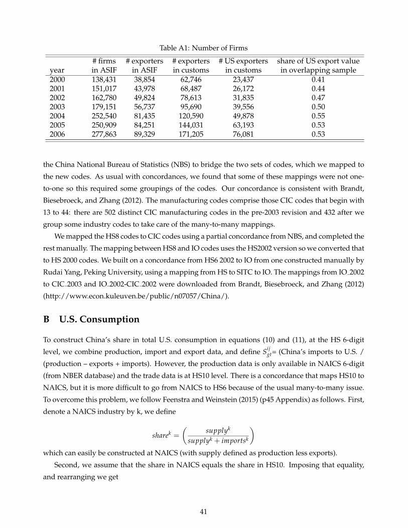
Table A1: Number of Firms

# firms # exporters # exporters # US exporters share of US export valueyear in ASIF in ASIF in customs in customs in overlapping sample2000 138,431 38,854 62,746 23,437 0.412001 151,017 43,978 68,487 26,172 0.442002 162,780 49,824 78,613 31,835 0.472003 179,151 56,737 95,690 39,556 0.502004 252,540 81,435 120,590 49,878 0.552005 250,909 84,251 144,031 63,193 0.532006 277,863 89,329 171,205 76,081 0.53

the China National Bureau of Statistics (NBS) to bridge the two sets of codes, which we mapped to

the new codes. As usual with concordances, we found that some of these mappings were not one-

to-one so this required some groupings of the codes. Our concordance is consistent with Brandt,

Biesebroeck, and Zhang (2012). The manufacturing codes comprise those CIC codes that begin with

13 to 44: there are 502 distinct CIC manufacturing codes in the pre-2003 revision and 432 after we

group some industry codes to take care of the many-to-many mappings.

We mapped the HS8 codes to CIC codes using a partial concordance from NBS, and completed the

rest manually. The mapping between HS8 and IO codes uses the HS2002 version so we converted that

to HS 2000 codes. We built on a concordance from HS6 2002 to IO from one constructed manually by

Rudai Yang, Peking University, using a mapping from HS to SITC to IO. The mappings from IO 2002

to CIC 2003 and IO 2002-CIC 2002 were downloaded from Brandt, Biesebroeck, and Zhang (2012)

(http://www.econ.kuleuven.be/public/n07057/China/).

B U.S. Consumption

To construct China’s share in total U.S. consumption in equations (10) and (11), at the HS 6-digit

level, we combine production, import and export data, and define Sijgt= (China’s imports to U.S. /

(production – exports + imports). However, the production data is only available in NAICS 6-digit

(from NBER database) and the trade data is at HS10 level. There is a concordance that maps HS10 to

NAICS, but it is more difficult to go from NAICS to HS6 because of the usual many-to-many issue.

To overcome this problem, we follow Feenstra and Weinstein (2015) (p45 Appendix) as follows. First,

denote a NAICS industry by k, we define

sharek =

(supplyk

supplyk + importsk

)which can easily be constructed at NAICS (with supply defined as production less exports).

Second, we assume that the share in NAICS equals the share in HS10. Imposing that equality,

and rearranging we get

41

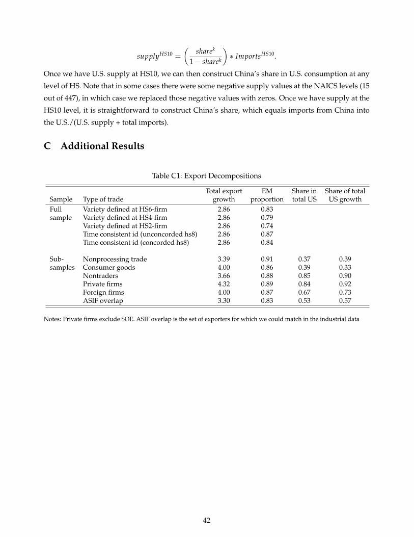
supplyHS10 =

(sharek

1− sharek

)∗ ImportsHS10.

Once we have U.S. supply at HS10, we can then construct China’s share in U.S. consumption at any

level of HS. Note that in some cases there were some negative supply values at the NAICS levels (15

out of 447), in which case we replaced those negative values with zeros. Once we have supply at the

HS10 level, it is straightforward to construct China’s share, which equals imports from China into

the U.S./(U.S. supply + total imports).

C Additional Results

Table C1: Export Decompositions

Total export EM Share in Share of totalSample Type of trade growth proportion total US US growthFull Variety defined at HS6-firm 2.86 0.83sample Variety defined at HS4-firm 2.86 0.79

Variety defined at HS2-firm 2.86 0.74Time consistent id (unconcorded hs8) 2.86 0.87Time consistent id (concorded hs8) 2.86 0.84

Sub- Nonprocessing trade 3.39 0.91 0.37 0.39samples Consumer goods 4.00 0.86 0.39 0.33

Nontraders 3.66 0.88 0.85 0.90Private firms 4.32 0.89 0.84 0.92Foreign firms 4.00 0.87 0.67 0.73ASIF overlap 3.30 0.83 0.53 0.57

Notes: Private firms exclude SOE. ASIF overlap is the set of exporters for which we could match in the industrial data

42

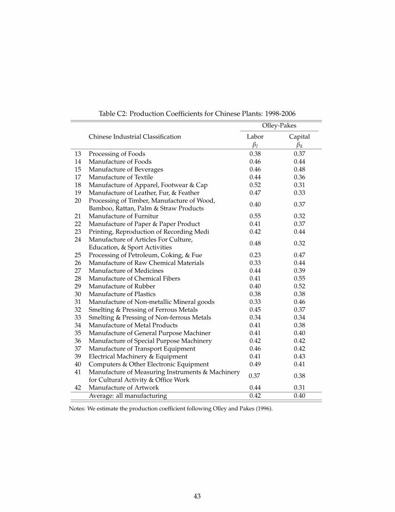
Table C2: Production Coefficients for Chinese Plants: 1998-2006

Olley-Pakes

Chinese Industrial Classification Labor Capitalβl βk

13 Processing of Foods 0.38 0.3714 Manufacture of Foods 0.46 0.4415 Manufacture of Beverages 0.46 0.4817 Manufacture of Textile 0.44 0.3618 Manufacture of Apparel, Footwear & Cap 0.52 0.3119 Manufacture of Leather, Fur, & Feather 0.47 0.3320 Processing of Timber, Manufacture of Wood, 0.40 0.37Bamboo, Rattan, Palm & Straw Products21 Manufacture of Furnitur 0.55 0.3222 Manufacture of Paper & Paper Product 0.41 0.3723 Printing, Reproduction of Recording Medi 0.42 0.4424 Manufacture of Articles For Culture, 0.48 0.32

Education, & Sport Activities25 Processing of Petroleum, Coking, & Fue 0.23 0.4726 Manufacture of Raw Chemical Materials 0.33 0.4427 Manufacture of Medicines 0.44 0.3928 Manufacture of Chemical Fibers 0.41 0.5529 Manufacture of Rubber 0.40 0.5230 Manufacture of Plastics 0.38 0.3831 Manufacture of Non-metallic Mineral goods 0.33 0.4632 Smelting & Pressing of Ferrous Metals 0.45 0.3733 Smelting & Pressing of Non-ferrous Metals 0.34 0.3434 Manufacture of Metal Products 0.41 0.3835 Manufacture of General Purpose Machiner 0.41 0.4036 Manufacture of Special Purpose Machinery 0.42 0.4237 Manufacture of Transport Equipment 0.46 0.4239 Electrical Machinery & Equipment 0.41 0.4340 Computers & Other Electronic Equipment 0.49 0.4141 Manufacture of Measuring Instruments & Machinery 0.37 0.38

for Cultural Activity & Office Work42 Manufacture of Artwork 0.44 0.31

Average: all manufacturing 0.42 0.40

Notes: We estimate the production coefficient following Olley and Pakes (1996).

43

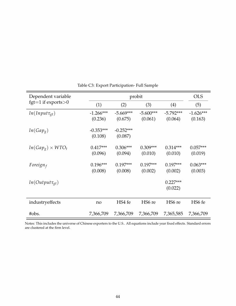
Table C3: Export Participation- Full Sample

Dependent variablefgt=1 if exports>0

probit OLS

(1) (2) (3) (4) (5)

ln(Inputτgt) -1.266*** -5.669*** -5.600*** -5.792*** -1.626***(0.236) (0.675) (0.061) (0.064) (0.163)

ln(Gapg) -0.353*** -0.252***(0.108) (0.087)

ln(Gapg)×WTOt 0.417*** 0.306*** 0.309*** 0.314*** 0.057***(0.096) (0.094) (0.010) (0.010) (0.019)

Foreign f 0.196*** 0.197*** 0.197*** 0.197*** 0.063***(0.008) (0.008) (0.002) (0.002) (0.003)

ln(Outputτgt) 0.227***(0.022)

industryeffects no HS4 fe HS6 re HS6 re HS6 fe

#obs. 7,366,709 7,366,709 7,366,709 7,365,585 7,366,709

Notes: This includes the universe of Chinese exporters to the U.S.. All equations include year fixed effects. Standard errorsare clustered at the firm level.

44