Embed Size (px)
Citation preview

Handbook of the Economics of Finance © 2013 Elsevier B.V. All rights reserved.http://dx.doi.org/10.1016/B978-0-44-459406-8.00021-4 1397
CHAPTER
Household Finance: An Emerging Field*
21
∗ We are very grateful to Nicholas Barberis, Laurent Calvet, John Campbell, James Choi, Steven Davis, Anna Dreber, Kenneth French, Michael Haliassos, Tullio Jappelli, Juanna Joensen, Ulf von Lilienfeld-Toal, Matti Keloharju, Ralph Koijen, Samuli Knupfer, Nikolai Roussanov, Meir Statman, Laura Veldkamp, Alexander Michaelides, Stephan Siegel, Irina Telyukova, Luis Viceira, James Vickery, for very helpful comments. Maria Gustafsson and Timotheos Mavropoulos have provided extremely careful and dedicated research assistance during the preparation of this chapter.
Contents
1. The Rise of Household Finance 1398 1.1 Why a New Field? 1399 1.2 Why Now? 14012. Facts About Household Assets and Liabilities 1402 2.1 Components of Lifetime Wealth: Human Capital 1403 2.2 Components of Lifetime Wealth: Tangible Assets 1406 2.2.1 Who Owns Tangible Wealth? 1407 2.2.2 The Wealth Allocation in Real and Financial Assets 1407 2.2.3 The Financial Portfolio 1413 2.3 Liabilities 1417 2.4 Trends 1419 2.5 Overall Reliance on Financial Markets 1420 2.6 International Comparisons 14213. Household Risk Preferences and Beliefs: What Do We Know? 1424 3.1 Measuring Individual Risk Aversion 1425 3.1.1 Revealed Preference Approach 1425 3.1.2 Elicitation of Risk Preferences 1428 3.2 Determinants of Risk Attitudes 1432 3.2.1 Risk Aversion and Financial Wealth 1433 3.2.2 Other Determinants of Risk Preferences 1437 3.3 Time-Varying Risk Aversion? 1443 3.4 Heterogeneity in the Financial Wealth Elasticity of the Risky Share 1445 3.5 Ambiguity and Regret 1446 3.6 Beliefs 1449 3.7 Risk Aversion, Beliefs, and Financial Choices; Putting Merton’s Model to the Test 14504. Household Portfolio Decisions, from Normative Models to Observed Behavior 1452 4.1 Stock Market Participation 1453
Luigi Guisoa and Paolo SodinibaEinaudi Institute for Economics and Finance, Via Sallustiana 62-00187 Rome, ItalybDepartment of Finance, Stockholm School of Economics, Sveavägen 65, Box 6501, SE-113 83 Stockholm, Sweden

Luigi Guiso and Paolo Sodini1398
1. THE RISE OF HOUSEHOLD FINANCE
In his 2006 Presidential Address to the American Financial Association,1 John Campbell coined the name “Household Finance” for the field of financial economics that studies
1 Campbell (2006).
4.1.1 Participation Costs and the Stockholding Puzzle 1453 4.1.2 Non-Standard Preferences and Limited Stock Market Participation 1454 4.1.3 Beliefs and Stock Market Participation 1456 4.1.4 Limited Participation in Other Financial Instruments 1458 4.1.5 The Bottom Line on Participation Puzzles 1459 4.2 Portfolio Selection 1459 4.2.1 Diversification 1460 4.2.2 Under-Diversification, Information, Hedging, and Preferences 1464 4.2.3 Frequency and Profitability of Trading 1470 4.2.4 Delegation of Portfolio Management and Financial Advice 1472 4.3 Portfolio Rebalancing in Response to Market Movements 1475 4.4 Portfolio Rebalancing Over the Life-Cycle 1478 4.4.1 Earlier Frictionless Models 1480 4.4.2 Non-Tradable and Non-Insurable Labor Income 1481 4.4.3 Addressing Counterfactual Predictions 1483 4.4.4 Welfare Implications 1485 4.4.5 Other Factors 1486 4.4.6 What Does the Empirical Evidence Tell Us About the Portfolio Life-Cycle? 14895. Household Borrowing Decisions 1496 5.1 Liabilities of the Household Sector: Magnitudes and Trends 1496 5.2 Credit Availability 1496 5.3 Optimal Mortgage Choice 1499 5.3.1 Theories of Mortgage Choice 1499 5.3.2 Evidence on Mortgage Choice 1501 5.3.3 Repayment and Refinancing 1503 5.4 Defaulting on Mortgages 1505 5.4.1 A Basic Framework 1506 5.4.2 Evidence 1507 5.5 Credit Card Debt, Debate and Puzzles 15106. Conclusion 1512Appendix A. Data Sources and Notes 1514 A.1 Definitions of Variables in the 2007 Wave of the SCF 1514 A.2 Assumptions for Tables 1 and 2 1516 A.2.1 Current Savings 1516 A.2.2 Pension Savings 1516Appendix B. Computation of Human Capital 1517References 1519

Household Finance: An Emerging Field 1399
how households use financial instruments and markets to achieve their objectives.2 Even though household finance had been attracting substantial academic attention, at the time of the address it had not yet earned its own title and identity. Today, household finance is a thriving, vibrant, self-standing field.
Households rely on financial instruments in many instances. They pay for goods and ser-vices with a variety of means including cash, checks, and credit cards. They transfer resources inter-temporally to invest in durable goods and human capital, or to finance present and future consumption. They face, and need to manage, various risks related to their health and possessions. All these activities involve payment choices, debt financing, saving vehicles, and insurance contracts that require knowledge and information to be used. Households can personally collect the necessary information, or can rely on third-party advices. Alternatively, they can delegate to external experts the task of managing their finances.
How should households take all these decisions? How do they actually choose?Following the long tradition in economics of developing models that offer pre-
scriptions on how agents should optimally choose consumption and investment plans, normative household finance studies how households should choose when faced with the task of managing their finances. While in many instances it may be reasonable to expect that actual behavior does not deviate from what normative models prescribe, this is not necessarily true when it comes to financial decisions, which are often extremely com-plex. Normative models can then be viewed as benchmarks against which to evaluate the ability of households to make sound financial choices.
Positive household finance studies instead actual financial decisions taken by house-holds and contrasts them with the prescriptions of normative models. Deviations from recommendations could simply be mistakes and, as such, be potentially rectified with financial education and professional advice. Alternatively, they could be the result of behavioral biases and thus challenge the benchmarking role of normative models themselves.
In this chapter we review the evolution and most recent advances of household finance. Needless to say, the available space requires us to concentrate on some topics while leaving others outside the scope of the chapter. Even within this selection, we will likely, and regrettably, fail to fully account for important contributions to the field. If so, let us apologize in advance.
1.1 Why a New Field?Research in financial economics has traditionally been organized into asset pricing and corporate finance, with contributions in household finance typically classified within the field of asset pricing. One may thus wonder why we need a new field and why we
2 Interestingly, the term economics comes from the Ancient Greek o’κoνoμíα—the combination of o’κoç (“house”) and νóμooooooç (“custom” or “law”)—to mean the administration and management of a house(hold).

Luigi Guiso and Paolo Sodini1400
need it now. In this section we try to answer the first question and attempt to address the second in the next section.The size of the industry. As Tufano (2009) points out, the financial services and prod-ucts used by households constitute a substantial portion of the financial industry in all advanced countries. At the end of 2010, according to the FED flow of funds, the total value of assets held by US households was $72 trillion, of which $48 trillion were finan-cial assets and the rest tangible assets, mostly real estate. On the liability side, households have $14 trillion in debt, of which mortgages are the biggest component. These figures are larger than the total value of assets and liabilities held by corporations. Corporations have $28 trillion in assets, half in tangible and half in financial assets, and outstanding lia-bilities for $13 trillion. Hence, households hold twice as much assets and at least as much debt as corporations. To the extent that market size is a measure of importance, the finances of households deserve at least as much attention as the finances of corporations.Household specificities. Households have to take a number of decisions which are not the focus of asset pricing and corporate finance but are central to household finances and welfare. They have to manage means of payment (cash vs. credit cards), forms of debt (personal vs. collateralized loans, fixed vs. variable rates), insurance contracts (accident, property, health insurance), and financial intermediaries (financial advisors, money man-agers). Additionally, households have features that set them apart from other agents in the economy. Human capital, the main source of lifetime income for most households, is typically non-traded, carries substantial idiosyncratic and uninsurable risk, accumulates very slowly and is hard to predict. The rest of household wealth is tangible and is largely invested in illiquid assets, typically real estate and durables. Many households have lim-ited access to credit which impairs their ability to transfer resources inter-temporally and smooth consumption over time. The fraction of tangible wealth held in liquid assets is typically hard to manage since, to do it efficiently, households need to overcome information barriers and sustain transaction costs. Some of these features have long been incorporated in models of microeconomic behavior. Some, though recognized in the literature, have been identified within contexts not directly related to the finances of households, and have been modeled dispersedly in several strands of economics, such as banking, the economics of insurance or household economics. Some are simply ignored by standard economic models, even though they play an important role in constraining and shaping household financial decisions.Relevance of institutional environment. Household decisions and their outcomes are often shaped by the institutional environment in which they are taken. For instance, it would be hard to explain, without appealing to regulatory, historical and cultural reasons, why in some countries, such as the US, households mostly rely on fixed-rate mortgages and in others, such as the UK, they mostly use variable rates. The institutions that affect household financial decisions are largely ignored by corporate finance, since they are fundamentally different from the ones affecting corporate

Household Finance: An Emerging Field 1401
decisions, and are not the focus of asset pricing, which tend to concentrate on valu-ation principles.Financial sophistication. Many households appear to have only a limited ability to deal with financial markets and possess a poor understanding of financial instruments. “Financial sophistication”—the understanding of financial instruments and competence in taking sound financial decisions—is not only limited for many, but it is also very unevenly distributed across households. One of the challenges that household finance distinctively faces is to study financial sophistication and its impact on household deci-sions and welfare.Specific regulatory interventions. Financial products and services used by households might need to be regulated for reasons already identified in other markets, such as various types of externalities and information failures. However, some of the issues highlighted above call for specific regulatory frameworks aimed at protecting households from making mistakes and from being exploited by intermediaries aware of their limitations.3
Overall, in studying household financial decisions, household finance takes into account and emphasizes the heterogeneity of household characteristics and the variety of institutional environments in which households operate. It considers investment decisions but, unlike asset pricing, it has a more equally weighted perspective and does not focus on wealthier and more risk tolerant investors. It explores the financing of household consumption and investment but, unlike corporate finance, it does not deal with the separation of ownership and control, and the capital structure of corporations. Household finance is more concerned with the choices of the median, rather than the marginal household. Agents that take marginal decisions (such as wealthy individuals and corporate executives) are likely to be financially sophisticated, obtain high-quality professional advice, have preferential access to credit, and rely on other sources of income than human capital. As such, they constitute only the minority of agents whose behavior is investigated by household finance.
1.2 Why Now?The interest and popularity that household finance is currently experiencing contrasts with the space that it was traditionally given within financial economics. Three possible explanations may help to rationalize the emergence of household finance as a field on its own.Relevance of household financial decisions. Households are today more directly involved in financial decisions than in the past. This is partially due to the privatization of pension systems, the liberalization of loan markets, and the recent credit expansion experi-enced by many developed countries. In addition, financial innovation has considerably
3 See Campbell et al. (2011) for a recent and thoughtful treatment.

Luigi Guiso and Paolo Sodini1402
enlarged the set of financing and investment choices available to households. More households are more easily involved in more complex financial choices than ever before.Data availability. The advancement of the field has also been recently facilitated by an explosion in the availability of detailed and comprehensive data on household finances. Before the 1990s, micro-data on household financial behavior was avail-able mostly through surveys, such as the Survey of Consumer Finances (henceforth SCF) in the US, and it suffered from limited quality and lack of details. Surveys are notoriously inaccurate, especially on the wealthy, and cannot be too specific in order to maximize response rates and accuracy. During the 1990s, and especially during the first decade of the century, a number of administrative micro datasets collected by private entities (companies, banks, and brokerage houses) and public institutions (governments and regulatory authorities) became available. Researchers effectively earned the means of investigating theoretical predictions that could not be studied before, and to document empirical regularities that had been lacking theoretical micro-foundations.Cultural heritage. Tufano (2009) provides a thoughtful account of several reasons for why household finance traditionally received little attention by mainstream financial economists. One intriguing explanation traces back to a century-old split between business-related and consumer-related topics based on geography and gender. The first were traditionally taught at elite urban universities which prepared men to deal with business careers. The second were instead studied at rural-land universities and taught mostly to women as part of household studies. Tufano conjectures that this separation played a relevant role in slowing the emergence of household finance as a separate field in financial economics.
The rest of the chapter is organized as follows. Section 2 presents basic facts about household wealth components and liabilities with emphasis on their variation in the wealth distribution. Section 3 reviews the literature on risk preferences, their measure-ment, and their determinants in the cross section and over time. Section 4 focuses on the asset side of household balance sheets, and discusses household participation, portfolio choice, trading behavior, and rebalancing over the business and the life-cycle. Section 5 concentrates on the liability side and reviews the literature on mortgages and credit card debt. Section 6 concludes.
2. FACTS ABOUT HOUSEHOLD ASSETS AND LIABILITIES
Who owns wealth? In which asset classes do households invest? What is the composi-tion of household financial portfolios? How many households have liabilities? Which forms of liabilities are more commonly chosen by households? Has the aggregate bal-ance sheet of the household sector changed over time? In this section we try to answer

Household Finance: An Emerging Field 1403
these questions and provide background descriptive information on household assets and liabilities by using the 2007 wave of the SCF.4 The section also provides an intro-duction to the topics encountered in the rest of the chapter and is organized as follows. We start by looking at the asset side of household balance sheets by considering first human capital, and then tangible wealth disaggregated into various real and financial asset classes. We then move to the liability side and study how various types of liabilities vary in the cross section of household wealth. The section concludes by presenting trends from previous waves of the SCF, and by outlining comparisons with countries other than the US.
2.1 Components of Lifetime Wealth: Human CapitalHouseholds can count on two main types of resources over their lifetime: tangible wealth, accumulated from savings or inheritance, and human capital. In this section we describe the main features of human capital and document how it varies with age and in relation to total wealth in the cross section of the 2007 wave of the SCF.
Human capital represents the stock of individual attributes—such as skills, person-ality, education, and health—embodied in the ability to earn labor income. It can be defined as the present discounted value of the flows of disposable labor income that an individual expects to earn over the remaining lifetime. Formally, the stock of human capital Ha of a household of age a is given by
where ya+τ is (uncertain) labor income at age a + τ , β the discount factor, T lifetime horizon and Ea the expectation operator at age a. Human capital has a number of note-worthy features that can potentially affect the way households choose their financial portfolios, manage their transaction accounts, buy insurance, and access credit.
First, human capital is accumulated slowly through formal education or working experience. Over the life-cycle, it reaches its highest level early in life and then declines as the number of earning years left and the flow of expected income decline.
Second, the value of human capital is hard to assess since it requires predicting earn-ings over the whole remaining lifetime, undoubtedly a daunting task given the uncer-tainty about future career prospects, health conditions, future individual and aggregate productivity, employments status, and any other contingency that might influence future earnings.
4 We refer the reader to the data appendix for the precise definitions and sources of the quantities we use in this section.
(2.1)Ha = Ea
T∑
τ=a
βτ−aya+τ ,

Luigi Guiso and Paolo Sodini1404
Third, human capital is not tradable and cannot be easily liquidated. This implies that human capital is hard to use as collateral and households cannot easily access credit markets in the absence of other forms of wealth. As a consequence, for most households and particularly for the poor, human capital represents the main component of their total wealth.
Finally, the uncertainty that characterizes future earnings makes the return to human capital risky. Most importantly, human capital represents a source of background risk – a risk that an individual has to bear and cannot be avoided-since it cannot be typically insured outside the provisions offered by public unemployment insurance schemes, and it cannot be liquidated. As we will see in Section 3, background risk influences an investor’s risk taking behavior and, thus, portfolio choice. The return on human capital may also co-vary with the stock market, an issue that has recently received attention to try to explain the reluctance to invest in stocks. However, the evidence suggests that the return on human capital is uncorrelated (or at least poorly correlated) with stock market returns. Hence, human capital can be viewed, from a portfolio allocation per-spective, as a “risk free bond”. This feature should affect the willingness to undertake financial risk and proves to be a critical factor for understanding portfolio rebalancing over the life-cycle. We will review the empirical and theoretical literature on these issues in Section 4.4.
Figure 1 shows estimates of the pattern of human capital over the life-cycle com-puted from the 2007 SCF for three educational groups. We report the details of the estimation in the appendix. Human capital is high for the young, who still have a long working life ahead of them, and low for the old, who will be soon or have already retired. It is higher at all ages for households with higher levels of education. In the very early stage of the life-cycle, the value of human capital for an individual with a college degree is around three million US dollars, compared to around one million for a person with less than high school education. Education not only influences the level but also the profile of human capital over the life-cycle. If earnings do not vary with age or grow little, as it is the case for individuals with low education, human capital peaks at the beginning of the working life and monotonically declines thereafter. If earnings grow very fast early in life, as happens with workers with high education, the peak in the stock of human capital may occur somewhat earlier over the life-cycle and decline thereafter-as shown in the figure.
Since human capital cannot be traded, liquidated, or used as collateral, most households accumulate tangible wealth mainly through savings. As a consequence, the proportion of household wealth held in human capital has a life-cycle pattern even more pronounced than that of human capital itself. For the typical household, human capital is the largest form of wealth early in life, when few savings have been accumulated. It progressively loses importance until retirement age when most

Household Finance: An Emerging Field 1405
households stop accumulating assets. Background risk is then particularly relevant for the young who have very little buffer savings and have still a long horizon over which earnings can be affected by persistent labor income shocks. Figure 2 shows the ratio of human capital to total wealth, defined as the sum of human capital and all forms of tangible wealth. Since, for most people, labor income is the primary source of wealth at the beginning of the working life, the proportion of wealth held in human capital is around one, and remarkably similar across education groups at the begin-ning of the life-cycle. The proportion declines monotonically for all groups as they age, both because they begin saving and accumulating tangible assets, and because human wealth starts declining. However, the decline rate is much faster for house-holds with higher education. At ages around 55, households with primary education have a stock of human capital that is still above 80% of total wealth, while, for those with college education, the fraction is around 60%. This is because more educated households face a faster declining stock of human capital and are able to accumulate tangible wealth faster.
0
500
1000
1500
2000
2500
3000
3500
4000
4500
24 26 28 30 32 34 36 38 40 42 44 46 48 50 52 54 56 58 60 62 64 66 68 70 72 74 76 78 80 82 84
1000
of 2
007
US
dolla
rs
Age
college high school no high school
Poly. (college) Poly. (high school) Poly. (no high school)
Figure 1 Age profile of human wealth. Average value of human capital in thousands of 2007 dollars over the life-cycle of households with college, high school and below high school education. Sample of US households in the 2007 wave of the SCF; the methodology is described in the appendix.

Luigi Guiso and Paolo Sodini1406
2.2 Components of Lifetime Wealth: Tangible AssetsThere are two broad categories of tangible assets in which individuals can invest their savings, real and financial assets. Real assets include residential and commercial property, durable goods (e.g. cars and vehicles), valuables (paintings, jewelry, gold, etc.) and private business wealth (the value of the assets involved in privately owned businesses). Financial assets include a very broad array of instruments ranging from cash and checking accounts to sophisticated derivative securities. Real and financial assets differ in several dimensions.
Real assets are illiquid. Real estate and business wealth are characterized by a high degree of specificity with only a small fraction of the existing stock on sale at each point in time (Piazzesi and Schneider, 2009). Durables are characterized by large informa-tion asymmetries and are affected by the classic lemons problem (Akerlof, 1970). Real assets thus involve high trading and legal costs, in addition to being taxed substantially in many countries.
The return on real assets is partially non-monetary. Residential property and durable goods provide consumption services on top of their own resale value (Piazzesi,
0
0.1
0.2
0.3
0.4
0.5
0.6
0.7
0.8
0.9
1
24 26 28 30 32 34 36 38 40 42 44 46 48 50 52 54 56 58 60 62 64 66 68 70 72 74 76 78 80 82 84Age
college high school no high school
Poly. (college) Poly. (high school) Poly. (no high school)
Figure 2 Age profile of the ratio of human to total wealth. Average ratio of the value of human capi-tal to total wealth over the life-cycle of households with college, high school and below high school education. Total wealth is the sum of human capital and tangible wealth. Sample of US households in the 2007 wave of the SCF; the methodology is described in the appendix.
Household Finance: An Emerging Field 1407
Schneider, and Tuzel, 2007), and private business wealth involves large non-monetary private benefits (Hamilton, 2000; Moskowitz and Vissing-Jorgersen, 2002). This feature makes it difficult to estimate the expected return and riskiness of real assets.
Real assets have the distinguishing feature that they are under the direct control of the owner and do not involve promises and claims. On the contrary, financial securities are claims over the income generated by real assets owned or controlled by someone else than the security holder. Hence, financial assets involve delegation of control that requires incentive contracts and monitoring mechanisms.
Financial assets are traded in markets typically more developed and liquid than real asset markets. Their number is very large and continuously increasing due to financial innovation. Since most financial assets are traded in organized markets, information on their past performance is public and is relatively easy to access.
Contrary to most real assets, financial securities differ greatly in complexity. The characteristics and the payoff structure of certain financial securities are extremely com-plex, and difficult to understand for many households. Additionally, information on the performance of financial assets is difficult to process and can be misleadingly interpreted. In this section we concentrate on tangible wealth and study its distribution in the 2007 wave of the SCF. We characterize the allocation between real and financial assets and then among various classes of financial securities.
2.2.1 Who Owns Tangible Wealth?Figure 3 reports the distribution of tangible wealth in the cross-section of households sampled in the 2007 SCF. The figure distinguishes between gross and net wealth, and between real and financial assets. The distribution is highly skewed. The average wealth in the top decile of the population is over 5,000 times larger than the average in the bottom decile. Such concentration of ownership implies that movements in the asset demand of a relatively small group of investors are likely to have large effects on asset prices. In Section 3 we will see that the frictionless neoclassical portfolio choice models predict that the portfolios of the rich are just a scaled up version of the portfolios of the poor. Models that postulate habit formation preferences or that integrate explicitly human capital imply that portfolio choice should instead depend on tangible wealth. Thus, uncovering the empirical relation between wealth and the portfolios of house-holds is a crucial issue in household finance that we start documenting in this section, and we will more thoroughly explore in Section 3, when we review the literature on the determinants of household financial risk taking.
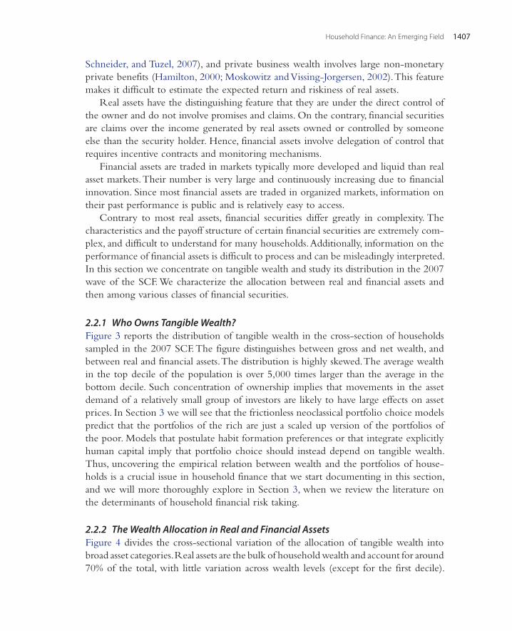
2.2.2 The Wealth Allocation in Real and Financial AssetsFigure 4 divides the cross-sectional variation of the allocation of tangible wealth into broad asset categories. Real assets are the bulk of household wealth and account for around 70% of the total, with little variation across wealth levels (except for the first decile).

Luigi Guiso and Paolo Sodini1408
By looking at these broad aggregates, one may conclude that the portfolio of the rich and that of the poor are quite similar. This similarity is only apparent.
A closer look at the composition of real assets already reveals quite striking differ-ences. The dotted line shows a marked hump in the fraction of real assets held as pri-mary residence. The very poor have no housing wealth, whereas housing is the primary form of wealth for the “middle class”. Among the very wealthy (i.e. those in the highest decile), the share invested in primary residence drops substantially to less than 60% (a finding that holds even if we consider all real estate investment, see Figure 5).
Interestingly, the rich seem to have a wealth allocation more similar to the poor than to the middle class. Again this similarity is only apparent and its source lies in the indivisibility of housing wealth. The very poor do not have enough wealth to afford a minimum living space. The very wealthy, instead, can afford to buy large, and possibly many, homes. To some extent they do, but they also own other types of real assets, nota-bly business wealth.
These variations in the composition of real asset holdings, besides revealing differ-ences in the overall asset allocation, may be relevant for understanding financial risk
10
100
1,000
10,000
100,000
1,000,000
10,000,000
1 2 3 4 5 6 7 8 9 10Deciles of gross tangible wealth
Total gross tangible wealth Net tangible wealth Real wealth Financial wealth
Figure 3 Wealth distribution. Average holdings of tangible wealth (gross and net), real wealth and financial wealth in dollars by deciles of gross tangible wealth. Sample of US households in the 2007 wave of the SCF; the variables are described in the appendix.

Household Finance: An Emerging Field 1409
taking. For instance, non-residential real estate may crowd out investment in risky financial securities, while residential holdings could act as a hedge for households who do not plan to move, an issue that we will study in more detail in Sections 3.2 and 4.4.
Figure 5 is more detailed than Figure 4 and reports the cross-sectional allocation of tangible wealth among six asset classes. Three are real and represent “vehicles”, “real estate”, and “private business” wealth. Three are financial and correspond to “cash”, “financial investment” and “other financial wealth”. “Cash” includes transaction accounts, such as checking and saving accounts, money market funds, cash and call accounts at brokerage houses, certificate of deposits and treasuries.5 “Financial invest-ment” contains current and retirement wealth in fixed income claims, directly and indirectly held equity as well as cash value life insurance. “Other financial wealth” has categories such as derivative securities, leases, and loans extended to friends and family relatives.6
5 Note that the SCF does not report cash held in notes and coins.6 See the appendix A for a detailed description of the variables.
0
0.1
0.2
0.3
0.4
0.5
0.6
0.7
0.8
0.9
0
0.1
0.2
0.3
0.4
0.5
0.6
0.7
0.8
0.9
1 2 3 4 5 6 7 8 9 10
Average share of prim
ary residence in real wealth
Ave
rage
sha
re o
f rea
l wea
lth in
tota
l wea
lth
Deciles of gross tangible wealth
Share of real wealth in total wealth Share of primary residence in real wealth
Figure 4 Broad wealth composition. Ratio of real to total gross wealth and fraction of real gross wealth held in primary residence by deciles of gross tangible wealth. Sample of US households in the 2007 wave of the SCF; the variables are described in the appendix.

Luigi Guiso and Paolo Sodini1410
The figure reveals remarkable differences in asset allocation across the population wealth distribution. Poor households have “cash and cars”, very little financial investment, mostly held in retirement wealth, and 5% invested in other financial assets. Closer exami-nation reveals that these are loans that the poor presumably make to family members and people belonging to their circle. This signals a more intense reliance on informal financial transactions among the poor, a symptom of deliberate non-participation or involuntary exclusion from formal markets. The proportion held in cash and vehicles—the wealth of the poor—decreases steadily for richer households, while that of real estate, driven by primary residence, increases sharply. Households with intermediate levels of wealth, besides holding most of their wealth in real estate, have a larger share of financial invest-ments. Financial investment is u-shaped above the third wealth decile, most likely due to the crowding out effect of real estate (Cocco, 2005; Yao and Zhang, 2005). Wealthy households have even more financial assets and in addition hold a larger fraction of their wealth in private businesses. Jointly these asset classes account for almost half of the wealth owned by households in the top decile. This is accompanied by a sharp decline of the share in real estate which amounts to less than half of the tangible wealth of the rich.
0
0.1
0.2
0.3
0.4
0.5
0.6
0.7
0.8
1 2 3 4 5 6 7 8 9 10
Ave
rage
sha
re o
f tot
al a
sset
s
Deciles of gross tangible wealth
Cash Vehicles Real estate Business Financial investment Other financial
Figure 5 Wealth composition. Allocation of tangible wealth in cash, vehicles, real estate, private busi-ness, financial investment and other financial assets, by deciles of gross tangible wealth. Sample of US households in the 2007 wave of the SCF; the variables are described in the appendix.

Household Finance: An Emerging Field 1411
The mean values of Figure 5 are calculated also on non-participants. Figure 6 shows participation rates—the fraction of households that invest in a certain asset class—for the same asset classes of Figure 5.
The most remarkable feature is that participation in all asset classes, except private business, increases sharply with wealth. At the lowest decile, participation is low in all asset classes and at intermediate levels for cash and vehicles.7 The rich, instead, tend to participate in all markets and half of the richest engage in private businesses. There is however heterogeneity across asset classes which may partly reflect differences in partici-pation costs. The poor own cash and vehicles as soon as their wealth turns positive. Ownership of housing is triggered by wealth in excess of the 4th decile. Interestingly, financial investment is higher than participation in housing below the 25th percentile, an implication of the indivisibility of real estate ownership.
Figure 7 shows asset allocations conditional on participation. Since, for each asset class, the share is computed among the participants in that asset class, and the group
7 As previously mentioned, the SCF does not report cash held in notes and coins.
0
0.1
0.2
0.3
0.4
0.5
0.6
0.7
0.8
0.9
1
1 2 3 4 5 6 7 8 9 10
Shar
e of
pop
ulat
ion
hold
ing
asse
t
Deciles of gross tangible wealth
Cash Vehicles Real estate Business Financial investment Other financial
Figure 6 Wealth participation. Fraction of households with positive asset holdings of cash, vehicles, real estate, private business, financial investment and other financial assets, by deciles of gross tan-gible wealth. Sample of US households in the 2007 wave of the SCF; the variables are described in the online appendix.

Luigi Guiso and Paolo Sodini1412
of participants differs across assets, the shares do not sum to one within each wealth decile. Interestingly, the poor tend to have highly concentrated wealth holdings. Their conditional shares are all high (except private business) and quickly decline as wealth increases. Once wealth exceeds the third decile, conditional allocations appear somewhat more stable. There are, however, some noteworthy patterns. First, similarly to Figure 5, the conditional share in real estate is hump-shaped and declines from 80% among those in the third wealth decile to 45% for those in the top decile. Second, the very poor have no investments in private businesses even though its proportion increases sharply at low wealth and it reaches 30% for households in the third wealth decile. For richer households, the share invested in private businesses is u-shaped, very rich and relatively poor entrepreneurs hold a comparable share of their tangible wealth in their private business activity. However, unlike the poor, the wealthy participate in all asset classes and are thus better able to absorb the idiosyncratic risk of their private business. Third, the few poor households who hold a financial investment, hold a very large portion of wealth in it. Otherwise, the share of wealth in financial investments is u-shaped (prob-ably due to the crowding out effect of real estate) and increases from the fifth decile of
0
0.1
0.2
0.3
0.4
0.5
0.6
0.7
0.8
0.9
1
1 2 3 4 5 6 7 8 9 10
Ave
rage
sha
re o
f tot
al a
sset
s
Deciles of gross tangible wealth
Cash Vehicles Real estate Business Financial investment Other financial
Figure 7 Conditional wealth composition. Allocation of tangible wealth in various asset classes among households with positive holdings in the asset class, by deciles of gross tangible wealth. Sample of US households in the 2007 wave of the SCF; the variables are described in the appendix.

Household Finance: An Emerging Field 1413
the wealth distribution. In Section 4.2.1, we will study the level of diversification house-holds achieve within their financial portfolio and argue that diversification in financial assets is positively affected by household wealth. Figure 7 suggests that poor households seem to hold undiversified holdings even when we consider broader categories of both real and financial assets. In the next section we restrict our attention to financial wealth and describe the cross-sectional variation in financial portfolio composition across the wealth distribution.
2.2.3 The Financial PortfolioAs shown in Figure 7, residential real estate represents the largest wealth component for the vast majority of households that can afford to buy it. Since, for most of these house-holds, all real estate wealth is tied in their own home, housing wealth is rarely transacted in response to transitory income or wealth shocks. As a consequence, empirical applica-tions of portfolio models tend to focus on the composition of financial wealth and treat housing as a source of background risk; i.e. a risk that cannot be avoided.8 In this sec-tion we follow this tradition and focus on the cross-sectional variation in the allocation of financial wealth.
Figure 8 shows the average shares of current and retirement financial wealth invested in five assets classes, cash, fixed income instruments, equity held either directly or indi-rectly (e.g. through mutual funds), cash value life insurance,9 and a residual category of other current financial assets.
The most striking feature is that the portfolio share in equity increases steadily with the level of investor wealth, while that in cash—the safe asset—declines markedly. Among households in the first wealth decile, cash accounts for over 80% of financial wealth and equity less than 5%. Among households in the top decile, cash amounts to only 20% and equity 50% of the portfolio. We will study the relation between financial risk taking and wealth in Section 3. For the moment we would like to highlight that, even when considering only financial assets, the portfolio of the rich is far from being a scaled up version of that of the poor.
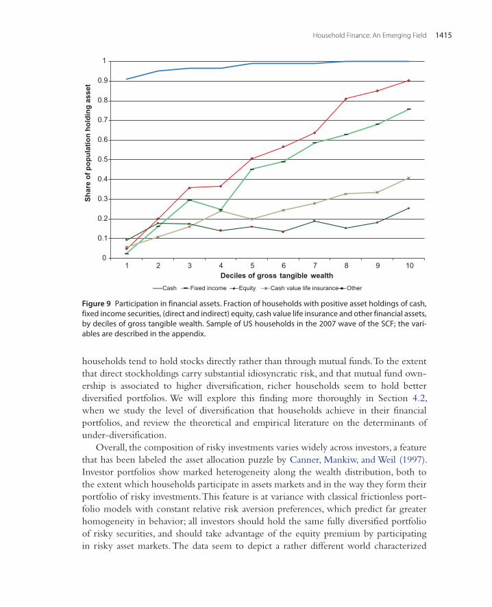
Figure 9 reports information on participation rates in the same financial assets classes of Figure 8. We can draw three observations from this figure. First, with the exception of cash, participation in financial assets is limited for households below median wealth. Second, participation strongly increases with the level of wealth for all
8 We refer the reader to Section 3 for a review of the literature on the effect of background risk on financial risk taking.
9 Cash value life insurance is a life insurance policy that builds up cash value over time, for example, through a guarantee interest on the cash value of the account. It is sometimes called “whole life”, “straight life”, or “universal life” policy. It is different from a traditional “term” policy which instead pays claim only upon early premature death.

Luigi Guiso and Paolo Sodini1414
financial asset classes. This is particularly true for equity and fixed income. Third, even though participation is much higher for the wealthy, there is limited participation in each asset class even among the richest households. For instance, 10% of the wealthiest households do not hold equity. Limited participation is puzzling, particularly for high levels of wealth, and in Section 4.1 we review the evolution of the large literature trying to reconcile the empirical findings with the predictions of optimal portfolio choice models.
For current financial wealth, but not for retirement savings, the SCF distinguishes between direct and indirect equity holdings.10Figure 10 reports how the components of current financial investment vary across wealth deciles. Directly and indirectly held stocks carry a much larger weight in the investment portfolio of the wealthy than in that of the poor while the opposite is true for fixed income. Interestingly, poorer
10 Individual stock ownership is classified as direct equity holding. Equity mutual fund ownership is considered indirect equity holding.
0
0.1
0.2
0.3
0.4
0.5
0.6
0.7
0.8
0.9
1 2 3 4 5 6 7 8 9 10
Ave
rage
sha
re o
f fin
anci
al a
sset
s
Deciles of gross tangible wealth
Cash Fixed income Equity Cash value life insurance Other
Figure 8 Composition of the financial portfolio. Allocation of financial wealth in cash, fixed income, equity (directly and indirectly), cash value life insurance and other financial assets, by deciles of gross tangible wealth. Sample of US households in the 2007 wave of the SCF; the variables are described in the appendix.
Household Finance: An Emerging Field 1415
households tend to hold stocks directly rather than through mutual funds. To the extent that direct stockholdings carry substantial idiosyncratic risk, and that mutual fund own-ership is associated to higher diversification, richer households seem to hold better diversified portfolios. We will explore this finding more thoroughly in Section 4.2, when we study the level of diversification that households achieve in their financial portfolios, and review the theoretical and empirical literature on the determinants of under-diversification.
Overall, the composition of risky investments varies widely across investors, a feature that has been labeled the asset allocation puzzle by Canner, Mankiw, and Weil (1997). Investor portfolios show marked heterogeneity along the wealth distribution, both to the extent which households participate in assets markets and in the way they form their portfolio of risky investments. This feature is at variance with classical frictionless port-folio models with constant relative risk aversion preferences, which predict far greater homogeneity in behavior; all investors should hold the same fully diversified portfolio of risky securities, and should take advantage of the equity premium by participating in risky asset markets. The data seem to depict a rather different world characterized
0
0.1
0.2
0.3
0.4
0.5
0.6
0.7
0.8
0.9
1
1 2 3 4 5 6 7 8 9 10
Shar
e of
pop
ulat
ion
hold
ing
asse
t
Deciles of gross tangible wealthCash Fixed income Equity Cash value life insurance Other
Figure 9 Participation in financial assets. Fraction of households with positive asset holdings of cash, fixed income securities, (direct and indirect) equity, cash value life insurance and other financial assets, by deciles of gross tangible wealth. Sample of US households in the 2007 wave of the SCF; the vari-ables are described in the appendix.

Luigi Guiso and Paolo Sodini1416
by substantial heterogeneity of behaviors. Understanding it is one of the challenges of household finance. In Section 4.2 we review the recent developments in understanding the risky components of household financial portfolios.
Figure 11 reports retirement portfolio allocations across three types of assets, namely, pension income, employer equity, and non-employer equity (as well as a residual cate-gory “other retirement”). Quite interestingly, except possibly for the two bottom and the two top deciles, the allocation of pension assets between equity and fixed income is quite similar across households with different wealth levels and it is close to an equal share rule.11 One important departure, however, is the relatively high weight of employer equity among the poor, which we will revisit in Section 4 when we try to understand whether households try to hedge their labor income risk.
11 Poorer households have a large fraction of pension wealth invested in other retirement assets. These are pension assets, other than fixed income and equity, mostly held in retirement accounts at the current employer, and include any of the following categories: real estate, hedge funds, annuities, mineral rights, business investment N.E.C, life insurance, non-publically traded business or other such investment. Unfortunately it is not possible to distinguish further among these categories in the SCF.
0
0.1
0.2
0.3
0.4
0.5
0.6
0.7
0.8
1 2 3 4 5 6 7 8 9 10
Ave
rage
sha
re o
f cur
rent
fina
ncia
l inv
estm
ent
Deciles of gross tangible wealthFixed income Directly held equity Indirectly held equity Cash value life insurance Other
Figure 10 Composition of current financial wealth. Allocation of current financial wealth in cash, fixed income, equity (directly and indirectly), cash value life insurance and other financial assets, by deciles of gross tangible wealth. Sample of US households in the 2007 wave of the SCF; the variables are described in the appendix.

Household Finance: An Emerging Field 1417
2.3 LiabilitiesFor many households access to the credit market is crucial to achieve a number of goals such as investing in human capital, smoothing consumption over time or pur-chasing a home early in life. Households can raise debt in a variety of ways. They can apply for a mortgage, use their credit card or obtain a consumer loan. Figures 12 and 13 report debt reliance for different levels of wealth. The average values in Figure 12 are calculated as shares of income, including households that do not borrow or borrow only through certain types of debt. Figure 13 reports the corresponding participation rates. Figure 14 reports values conditional on participation in the debt category.
There are a number of points worth noticing. First, different types of debt matter at different levels of wealth. Poorer households are less likely to have mortgage debt, whereas 70% of households above median wealth have a mortgage. Households in the third decile of wealth rely on student and consumer loans more than wealthier house-holds. Reliance on credit card debt is higher for households within the second to the eighth deciles of the wealth distribution.
0
0.1
0.2
0.3
0.4
0.5
0.6
0.7
1 2 3 4 5 6 7 8 9 10
Ave
rage
sha
re o
f pen
sion
fina
ncia
l inv
estm
ent
Deciles of gross tangible wealthFixed income Non-employer equity Employer equity Other
Figure 11 Composition of pension wealth. Allocation of pension financial wealth in fixed income, non-employer and employer equity by deciles of gross tangible wealth. Sample of US households in the 2007 wave of the SCF; the variables are described in the appendix.

Luigi Guiso and Paolo Sodini1418
Second, the way participation rates and debt to income ratios change with wealth is not uniform across categories. Participation increases with wealth for mortgages (quite steeply for relatively poor households). It is hump shaped for credit card and consumer debt, whereas it declines with wealth for education loans. Similar patterns hold for unconditional debt to income ratios. Conditional on participation, instead, debt to income ratios for personal loans tend to be higher for poorer households whereas the opposite pattern can be observed for mortgages.
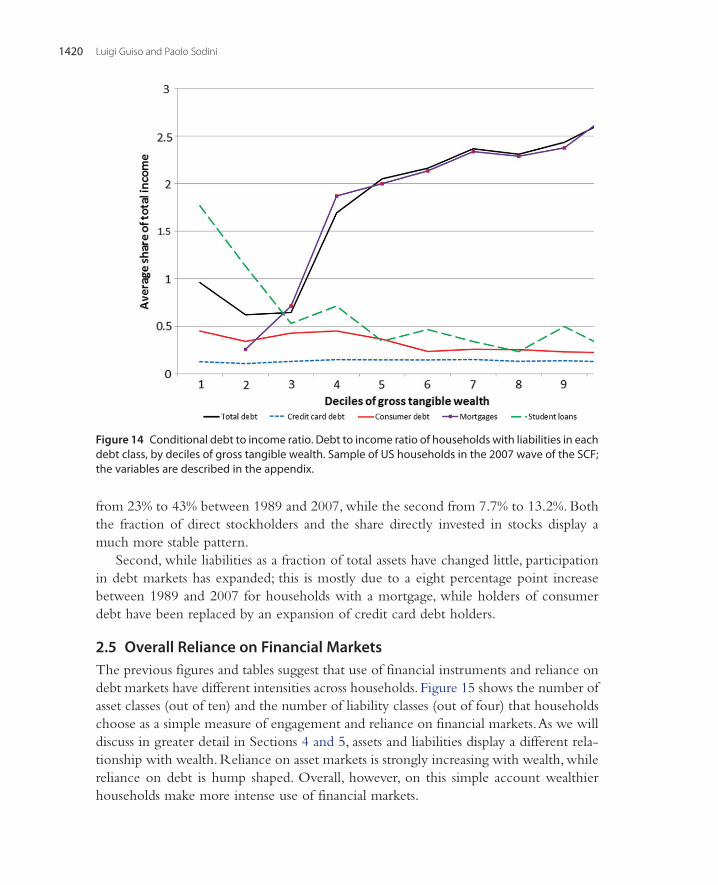
Third, among households with a mortgage, the richest half holds on average a mort-gage at least twice as large as income (Figure 14). It is then not surprising that consider-able academic attention has been devoted to how households choose among mortgage types (e.g. fixed versus variable rate). We refer the reader to Section 5.3 for a review of the theoretical and empirical literature on optimal mortgage choice.
Finally, the joint consideration of Figures 6 and 13 reveal that many households with intermediate levels of wealth hold both substantial liquid assets and personal loans in their balance sheets. As a result, they effectively pay very high interest rates without
0
0.5
1
1.5
2
2.5
1 2 3 4 5 6 7 8 9 10
Ave
rage
sha
re o
f tot
al in
com
e
Deciles of gross tangible wealth
Total debt Credit card debt Consumer debt Mortgages Student loans
Figure 12 Debt to income ratio. Debt to income ratio for various classes of debt by deciles of gross tangible wealth. Sample of US households in the 2007 wave of the SCF; the variables are described in the appendix.

Household Finance: An Emerging Field 1419
an apparent need for it. Section 5.5 reviews the literature that tries to rationalize this seemingly puzzling behavior.
2.4 TrendsTable 1 reports the evolution over time of household assets and liabilities as fraction of total wealth, using waves of the SCF from 1989 to 2007. Table 2 shows the dynamics of the corresponding participation rates. These tables make it clear that all features we have documented for 2007—the prominence of real assets, particularly primary resi-dence; limited participation in asset markets, particularly in equity; and the diffusion of debt—are common to all previous waves of the SCF, implying that these key features of household finance are stable over time. However, they also highlight two important evolving patterns. First, financial portfolios have become “riskier”, as the average share of total financial assets held in equity has increased from 30.4% in 1989 to 52.7% in 2007, and participation in the equity market has gone up from 35.4% to 51.5% over the same period. This evolution is mostly due to increased equity participation through pension savings and current financial investment in mutual funds, the first has increased
0
0.1
0.2
0.3
0.4
0.5
0.6
0.7
0.8
0.9
1
1 2 3 4 5 6 7 8 9 10
Shar
e of
pop
ulat
ion
hold
ing
debt
Deciles of gross tangible wealthAny debt Credit card debt Consumer debt Mortgages Education loans
Figure 13 Participation in debt markets. Fraction of indebted households for various classes of debt by deciles of gross tangible wealth. Sample of US households in the 2007 wave of the SCF; the vari-ables are described in the appendix.
Luigi Guiso and Paolo Sodini1420
from 23% to 43% between 1989 and 2007, while the second from 7.7% to 13.2%. Both the fraction of direct stockholders and the share directly invested in stocks display a much more stable pattern.
Second, while liabilities as a fraction of total assets have changed little, participation in debt markets has expanded; this is mostly due to a eight percentage point increase between 1989 and 2007 for households with a mortgage, while holders of consumer debt have been replaced by an expansion of credit card debt holders.
2.5 Overall Reliance on Financial MarketsThe previous figures and tables suggest that use of financial instruments and reliance on debt markets have different intensities across households. Figure 15 shows the number of asset classes (out of ten) and the number of liability classes (out of four) that households choose as a simple measure of engagement and reliance on financial markets. As we will discuss in greater detail in Sections 4 and 5, assets and liabilities display a different rela-tionship with wealth. Reliance on asset markets is strongly increasing with wealth, while reliance on debt is hump shaped. Overall, however, on this simple account wealthier households make more intense use of financial markets.
Figure 14 Conditional debt to income ratio. Debt to income ratio of households with liabilities in each debt class, by deciles of gross tangible wealth. Sample of US households in the 2007 wave of the SCF; the variables are described in the appendix.

Household Finance: An Emerging Field 1421
2.6 International ComparisonsThe key features of household finances that we have highlighted for the US extend essentially to all developed countries, as documented in Guiso, Haliassos, and Jappelli (2002). The tendency of wealth to be concentrated among the richest, the broad
Table 1 Shares of assets and liabilities. Share of total gross wealth in various assets and liabilities for different waves of the SCF. The variables are described in the appendix 1989 1992 1995 1998 2001 2004 2007
Assets and liabilities as % of total assetsFinancial wealth
30.6 31.6 36.9 41.0 42.6 35.9 34.1
Cash 9.8 8.9 8.4 7.1 7.0 6.5 5.4Directly held equity
4.5 5.1 5.6 9.1 8.9 6.1 4.9
Fixed income 3.7 3.9 3.7 3.6 4.1 3.9 3.2Cash value life insurance
1.8 1.9 2.6 2.5 2.2 1.0 1.1
Pension equity 2.9 4.2 6.1 8.1 8.7 6.8 6.9Pension fixed income
3.9 4.2 4.4 3.5 3.9 5.0 4.7
Other pension assets
0.2 0.3 0.4 0.3 0.0 0.6 0.8
Other financial assets
1.9 1.4 1.8 1.4 1.2 0.8 0.9
Risky financial 9.3 11.1 15.7 22.5 24.2 18.1 18.0Risky financial % of financial assets
30.4 35.0 42.5 55.0 56.8 50.4 52.7
Real wealth 69.4 68.4 63.1 59.0 57.4 64.1 65.9Primary residence
30.2 31.3 29.3 27.3 26.8 31.7 31.4
Investment real estate
16.2 14.7 10.9 10.5 10.1 12.0 11.7
Debt 15.0 15.9 15.5 15.0 12.7 15.8 15.6Credit cards 0.3 0.5 0.6 0.5 0.4 0.4 0.5Consumer debt
2.3 1.5 1.5 1.6 1.3 1.4 1.1
Real estate debt
11.9 13.3 12.7 12.0 10.5 13.4 13.3
Loans for education
0.2 0.3 0.4 0.4 0.3 0.4 0.5

Luigi Guiso and Paolo Sodini1422
Table 2 Participation rates in assets and debt markets. Participation rates in various categories of assets and liabilities for the households sampled by different waves of the SCF. The variables are described in the appendix 1989 1992 1995 1998 2001 2004 2007
Ownership of assets and liabilities
Financial wealth
88.8 90.3 91.1 93.0 93.2 93.4 93.3
Cash 85.9 87.5 87.7 90.9 91.2 91.1 91.3Directly held equity
16.9 17.0 15.2 19.2 21.3 20.7 19.6
Indirectly held equity
7.7 9.9 12.6 17.6 19.4 16.8 13.2
Fixed income 9.7 10.3 8.3 10.1 9.9 10.5 7.9Cash value life insurance
35.5 34.9 32.0 29.6 28.0 24.2 23.0
Pension equity 22.9 29.2 33.7 40.0 44.0 41.1 43.1Pension fixed income
31.4 31.8 30.4 30.1 30.6 40.7 39.7
Other pension assets
2.5 3.3 5.1 2.3 1.1 3.7 7.0
Other financial assets
15.0 11.9 12.6 10.7 10.2 10.1 9.5
Risky financial 35.4 40.1 44.0 50.7 53.8 50.4 51.5Real wealth 89.3 90.8 90.9 89.9 90.7 92.5 92.0Primary residence
63.9 63.9 64.7 66.3 67.7 69.1 68.6
Investment real estate
20.3 19.4 18.0 18.6 16.8 18.1 19.0
Debt 72.6 73.4 74.7 74.3 75.4 76.5 77.1Credit cards 39.7 43.7 47.3 44.1 44.4 46.2 46.1Consumer debt
49.2 45.1 43.4 41.9 43.7 42.9 43.1
Real estate debt
41.9 41.8 43.2 45.2 46.4 49.2 50.3
Loans for education
8.9 10.7 11.9 11.3 11.5 13.4 15.2
Average no. of asset classes
3.7 3.9 3.8 4.0 4.1 4.2 4.1
Average no. of liability classes
1.4 1.4 1.5 1.4 1.5 1.5 1.5

Household Finance: An Emerging Field 1423
variation in assets shares across wealth deciles, the limited participation in various assets classes and its positive relation with wealth are common to all industrialized economies. For many purposes, researchers can then rely on data available from any developed country to study broad features of household finances. This is particularly convenient when adequate data may only be available in some countries. For instance, the Nordic countries, and Sweden in particular, have administrative data on house-hold wealth and all its components that is not available anywhere else and that is almost free of measurement error.12 In countries such as the US, the Netherlands, Italy and Spain there is a long tradition of collecting rich household finance surveys. In some cases, such as Italy, survey data can be merged with administrative data from intermediaries (e.g. Alvarez, Guiso and Lippi, 2012). The collection of household sur-vey data is now being extended to all the countries in the euro area through a specific
12 See, for example, Calvet, Campbell, and Sodini (2007a, 2007b) for the equivalent of Figures 3, 5, and 8.
0
1
2
3
4
5
6
7
1 2 3 4 5 6 7 8 9 10
Ave
rage
num
ber o
f cla
sses
Deciles of gross tangible wealthLiability classes Asset classes
Figure 15 Households reliance on financial and credit markets. Average number of asset and debt classes by deciles of gross tangible wealth. The asset classes are cash, vehicles, real estate, business, directly held equity, indirectly held equity, fixed income, pension equity, pension fixed income, cash value life insurance. The debt classes are credit card, consumer debt, education loans, mortgages. Sample of US households in the 2007 wave of the SCF; the variables are described in the appendix.

Luigi Guiso and Paolo Sodini1424
instrument—the Household Finance and Consumption Survey (HFCS)13—adminis-tered by the European Central Bank.
We should however recognize that, though the basic features of household finance are qualitatively similar across countries, their size often differs (Christelis, Georgarakos, and Haliassos, in press). The availability of comparable data across countries should thus be exploited to shed light on the role of institutional and regulatory differences in shap-ing households financial decisions. The field of international household finance is still in its infancy even though is likely to provide important insights on how households use financial markets to achieve their goals.
3. HOUSEHOLD RISK PREFERENCES AND BELIEFS: WHAT DO WE KNOW?
Risk preferences are a key ingredient in models of financial decisions. They play an essential role in modeling the demand for insurance, the choice of mortgage type, the frequency of stock trading, and the acquisition of financial information. In this section we review the large literature on the measurement and determinants of risk preferences in the context of household financial decisions.
Understanding investor risk preferences has several important implications. First, it offers guidance for the calibration of optimal portfolio choice models. Second, it can provide empirical micro-foundations to asset pricing models with heterogeneous agents. Third, it contributes to the asset pricing debate on time-varying risk aversion (Campbell, 2003). Fourth, it permits the assessment of the welfare costs of financial mistakes such as under-diversification, and non-participation in financial and insurance markets. Finally, it helps financial intermediaries to comply with investor protection regulations that require the measurement of risk preferences before providing financial advices (e.g. European Investment Service Directive—MiFID).
Risk preferences are central to theories of financial portfolio choice that build on the standard expected utility framework of Von Neumann and Morgenstern (2007). These models draw a direct relation between the fraction of financial wealth invested in risky assets—the portfolio risky share—and risk preferences. In the classical Merton (1969) model of consumption and portfolio choice, investor i’s optimal risky share ωi is
where Erei is the expected risk premium, σi is the return volatility of risky assets, and γi
the Arrow-Pratt degree of relative risk aversion. A pervasive assumption in the literature,
13 See http://www.ecb.int/home/html/researcher_hfcn.en.html.
(3.1)ωi =Ere
i
γiσ2i
,

Household Finance: An Emerging Field 1425
motivated by the fact that households have to hold the market portfolio in the aggregate, is that beliefs about risky assets are the same for all investors, Ere
i = Ere and σ 2i = σ 2. In
this case, the model yields the powerful implication that all heterogeneity in observed portfolio shares should be explained by differences in risk attitudes, which are captured in the model by the relative risk aversion parameter γi. Several theories build on (3.1) to identify the determinants of the relative risk aversion coefficient γi. For example, within the expected utility framework, if individual preferences display constant rela-tive risk aversion (CRRA), wealthy and poor investors should all have the same share of wealth invested in risky assets, ωi. If investors display decreasing relative risk aversion preferences (DRRA), instead, wealthier investors should invest a larger fraction of their wealth in risky assets.
We begin this section by discussing how to measure risk preferences. Researchers have followed two approaches. The revealed preference strategy infers relative risk aver-sion from observed household portfolio risky shares by reversing (3.1). Alternatively, risk preferences are elicited from subject behavior in experiments and answers to survey questionnaires.
We then review the literature on the determinants of risk preferences. First, we focus on wealth and other individual and environmental factors. Second, we report the most recent findings on whether and how risk aversion varies over time. Third, we study the sensitivity of financial risk taking in relation to household wealth. Fourth, we consider the role of non-standard preferences such as ambiguity aversion and regret. Finally, we discuss how we can measure beliefs and how they vary across households. We conclude by testing the Merton model (3.1) directly with data on household risk aversion, beliefs, and wealth.
3.1 Measuring Individual Risk AversionResearchers have followed two approaches to measuring household attitudes towards risk. The first is based on a revealed preference strategy that infers risk aversion from the portfolio risky share chosen by investors in real life. The second relies on the elici-tation of risk preferences from subject behaviors in experiments and answers to survey questionnaires.
3.1.1 Revealed Preference ApproachIn a seminal paper, Friend and Blume (1975) infer relative risk aversions from the household portfolio risky shares reported in surveys of the Federal Reserve Board.14
14 They use the 1962 and 1963 Federal Reserve Board Surveys of the Financial Characteristics of Consumers and Changes in Family Finances.

Luigi Guiso and Paolo Sodini1426
They follow a revealed preference approach by obtaining the risk aversion of investor i from (3.1).
We implement their methodology in Table 3 by using the 2007 US SCF and the 2007 Swedish Wealth Registry.
The estimates are obtained by assuming that the expected excess return Erei and
volatility σi are the same for all investors and are calibrated to the historical stock market estimates of 6.2% and 20%, respectively. The results are remarkably stable across the two countries. The median value of the relative risk aversion parameter γi is 3.5 in the US and 3.8 in Sweden. In both countries, more than three-fourth of households have a coefficient of relative risk aversion below 10—the maximum value considered plausible by Mehra and Prescott in their 1985 seminal paper on the equity premium puzzle. Table 3 shows that cross-sectional estimates of relative risk aversion coefficients are by far more reasonable than the ones necessary to rationalize the equity risk premium within the consumption of the CAPM framework. Coefficients many times greater than 10 are needed to justify the size of stock market risk premia around the globe (Campbell, 2003).15 However, it is important to bear in mind that the Friend-Blume approach is likely to understate risk aversion for at least two reasons. First, it assumes i.i.d. returns and thus uses short-run asset volatility as a proxy for long-run volatility. Second, it does not account for human capital which is of dominant importance for most households. We extensively review the effect of human capital on portfolio alloca-tion over the life-cycle in Section 4.4.
Table 3 is obtained under the assumption that all households invest the risky share of their financial wealth in the same fully diversified portfolio that reproduces the stock market. As we shall see in Section 4.2, the composition of household portfolios violates this assumption and thus the first two columns of Table 3 might hold incorrect esti-mates of γi. The Swedish data has the unique advantage of reporting security holdings at individual asset level and thus allows for measuring precisely the expected excess return Ere
i and volatility σi of households actual risky portfolios.16 The revised estimates are reported in the third column of Table 3. Risk aversion parameters are slightly lower with a median value of 3.1. Three-quarters of the sample have a coefficient of relative risk aversion lower than 6.9. Households appear somewhat less risk averse once the expected return and riskiness of their actual risky portfolios are taken into account. Since they have portfolios with lower Sharpe ratios Ere
i /σi than the market index,
γi =Ere
i
ωiσ2i
.
15 The cross-country variation is large. For instance, γi = 240 in the US and 59 in Canada.16 We use the International CAPM model of Calvet, Campbell, and Sodini (2007a) to estimate portfolio
expected returns.

Household Finance: An Emerging Field 1427
portfolio shares can be more easily rationalized within the basic Merton formula (3.1). However, the estimates obtained with the actual composition of the risky portfolio do not change considerably, an indication that the majority of households achieve good levels of diversification, as we shall see in Section 4.2.1.
Even though we have excluded from the two samples households with less than $100 invested in risky assets, some households hold very small risky shares and their coefficient of relative risk aversion is estimated at unreasonable levels.17 There are at least two explanations to this finding.
First, (3.1) does not consider how risk aversion varies with household characteristics, such as wealth, background risk, and demographics. We review in Section 3.2 the large and long-lasting literature devoted to filling this gap.
Second, we have assumed that our estimates of expected returns and volatilities, based on historical data, coincide with the beliefs of the households sampled. As we shall see in Section 3.5, households have substantially dispersed beliefs about stock market profitability and riskiness. Some might hold very negative views or might not even trust investing in products that entail portfolio delegation, such as mutual funds.
17 We exclude households with very low investment in risky assets to avoid estimates resulting from inertia and the 2007 low market valuation. In Table 3, the median would be 3.5, 4.6, and 3.3, from left to right. The 75th percentiles would be: 7.3, 13.1, and 8.0.
Table 3 Imputed Relative Risk Aversion Coefficient. Cross sectional distribution of relative risk aver-sion coefficients estimated with the revealed preference approach using observed risky shares. The first two columns assume investment in an asset with expected excess return of 6.2% and volatility of 20%, representing an internationally diversified market index. The third column uses the expect-ed returns and volatilities of the households observed portfolios estimated with the International CAPM model of Calvet, Campbell, and Sodini (2007a, 2007b). The first column uses the SCF, 2007. The second and third columns use the Swedish Wealth Registry, 2007. Households with investment in risky asset below $100 (SEK 640) are excluded
Relative risk aversion coefficient
Imputed risky portfolios (full diversification)
Observed risky portfolios
Percentiles US SCF Swedish wealth registry
1 1.6 1.6 0.35 1.6 1.7 0.710 1.8 1.9 1.025 2.2 2.4 1.850 3.5 3.8 3.175 7.1 8.6 6.990 16.4 24.9 17.895 30.8 50.1 34.699 136.4 189.6 132.3
Luigi Guiso and Paolo Sodini1428
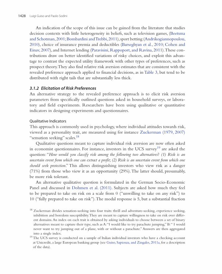
An indication of the scope of this issue can be gained from the literature that studies decision contexts with little heterogeneity in beliefs, such as television games, (Beetsma and Schotman, 2001; Bombardini and Trebbi, 2011), sport betting (Andrikogiannopoulou, 2010), choice of insurance premia and deductibles (Barseghyan et al., 2010; Cohen and Einav, 2007), and Internet lending (Paravisini, Rappoport, and Ravina, 2011). These con-tributions draw on better identified variations of risky choices, and exploit this advan-tage to contrast the expected utility framework with other types of preferences, such as prospect theory. They also find relative risk aversion estimates that are consistent with the revealed preference approach applied to financial decisions, as in Table 3, but tend to be distributed with right tails that are substantially less thick.
3.1.2 Elicitation of Risk PreferencesAn alternative strategy to the revealed preference approach is to elicit risk aversion parameters from specifically outlined questions asked in household surveys, or labora-tory and field experiments. Researchers have been using qualitative or quantitative indicators in designing experiments and questionnaires.
Qualitative IndicatorsThis approach is commonly used in psychology, where individual attitudes towards risk, viewed as a personality trait, are measured using for instance Zuckerman (1979, 2007) “sensation seeking” scales.18
Qualitative questions meant to capture individual risk aversion are now often asked in economist questionnaires. For instance, investors in the UCS survey19 are asked the question: “How would you classify risk among the following two alternatives? (1) Risk is an uncertain event from which one can extract a profit; (2) Risk is an uncertain event from which one should seek protection.” This allows distinguishing investors who view risk as a danger (71%) from those who view it as an opportunity (29%). The latter should, presumably, be more risk tolerant.
An alternative qualitative question is formulated in the German Socio-Economic Panel and discussed in Dohmen et al. (2011). Subjects are asked how much they feel to be prepared to take on risk on a scale from 0 (“unwilling to take on any risk”) to 10 (“fully prepared to take on risk”). The modal response is 5, but a substantial fraction
18 Zuckerman divides sensation-seeking into four traits: thrill and adventure-seeking, experience seeking, inhibition and boredom susceptibility. They are meant to capture willingness to take on risk over differ-ent domains. An index on each trait is obtained by asking individuals to choose between a set of binary alternatives meant to capture their type, such as A: “I would like to try parachute jumping,” B: “ I would never want to try jumping out of a plane, with or without a parachute.” Answers are then aggregated into a single index.
19 The UCS survey is conducted on a sample of Italian individual investors who have a checking account at Unicredit, a large European banking group (see Guiso, Sapienza, and Zingales, 2011a, for a description of the data).

Household Finance: An Emerging Field 1429
of individual answers are between 2 and 8. There is also a 7% mass who choose the extreme of 0, indicating a complete unwillingness to take on risk. A very small fraction of respondents report the extreme values of 9 or 10.
In a context closer to financial choices, the SCF elicits risk attitudes by asking indi-viduals: “Which of the following statements comes closest to the amount of financial risk that you are willing to take when you make your financial investment? (1) Take substantial financial risks expecting to earn substantial returns; (2) Take above average financial risks expecting to earn above average returns; (3) Take average financial risks expecting to earn average returns; (4) Not willing to take any financial risks”.
Figure 16 shows the distribution of the answers to this question in the 2007 SCF and in the 2007 UCS. Interestingly, even though the UCS survey has been conducted at the beginning of 2007 and the financial crisis affected the US earlier than Italy, the two distributions present substantial similarities. Very few (less than 5%) report they would take substantial financial risk even if compensated with high returns; most would take an average financial risk/average return combination.
Overall, these qualitative measures of risk attitudes suggest that most individuals view risk as a danger and are averse to it; but at the same time there is wide dispersion
0
10
20
30
40
50
60
Substantial risk & return
Above average risk and return
Average risk and return
No financial risk
% fr
eque
ncy
ITALY USA
Figure 16 Elicited risk aversion. Frequency distribution of a qualitative indicator of risk aversion obtained eliciting people preferences for different combinations of risk and return in Italy and the US. US values are obtained from the 2007 SCF; those for Italy from the 2007 UCS.

Luigi Guiso and Paolo Sodini1430
in attitudes towards risk. Some individuals are very uncomfortable with risk, but a significant fraction of the population is willing to take on risk if adequately com-pensated. The main advantage of these questions is that they are simple to ask and thus particularly suited for large surveys. Indeed, when asked, they result in very few non-responses. They have also been shown to predict risk-taking behavior in various domains (see for instance Dohmen et al., 2011, and Donkers, Melenberg and Soest, 2001) and can thus be used to sort investors into risk tolerance groups. The main drawback is that they do not distinguish between aversion to risk and perception of risk, hence some individuals may appear more risk-averse in the data because they have beliefs that place higher probabilities on adverse events. In addition, qualitative measures do not permit precise estimates of the Arrow-Pratt degree of relative risk aversion, γi, used in (3.1).
Quantitative MeasuresQuantitative measures try to deal with these issues by asking individuals to choose among specific risky choices and by eliciting their degree of relative risk aversion γi, under the assumption that they behave as expected utility maximizers. Guiso and Paiella (2008) recover estimates of absolute risk aversion by asking individuals in the SHIW (The Italian Survey of Households Income and Wealth) about their willingness to pay for an hypothetical lottery involving a gain of 5,000 euros with probability a half.20 Since relative risk aversion is equal to absolute risk aversion multiplied by wealth, esti-mates of relative risk aversion are problematic to obtain from the absolute parameters as they require assumptions on how to proxy for the relevant wealth measure. A more direct approach is instead used in Barsky et al. (1997), who elicit interval measures of relative risk aversion on respondents to the PSID. They ask subjects to choose between keeping their present job at the current salary forever and switching to (otherwise equivalent) jobs with uncertain lifetime earnings. Answers allow them to group the degree of relative risk aversion of the respondents into four intervals. They find that the average household has a coefficient of relative risk aversion around 4, in line with the estimates obtained with the Friend and Blume approach.21
The inferred quantitative measures obtained in these studies should be considered estimates of the risk aversion parameters of the respondents’ value functions, and should then depend on variables that affect willingness to take on risk, such as wealth and prox-ies for background risk. Since questions on risk aversion are typically included in gen-eral economic surveys, quantitative measures can be related to household observables to study the properties of the risk aversion function, in particular how it relates to wealth,
20 Hartog, Ferrer-i-Carbonell, and Jonker (2002) use a similar approach in a sample of Dutch accountants.21 Barsky et al. (1997) mostly report coefficients of relative risk tolerance which are the inverse of relative
risk aversion.

Household Finance: An Emerging Field 1431
stable demographic characteristics and the economic environment. Furthermore, since general surveys collect data on financial risk taking, one can test the predictive power of these measures on observed financial choices.
However, these quantitative measures of risk aversion have drawbacks too. First, when asked about willingness to pay, individuals tend to underreport, which overesti-mates their true risk aversion (Kachelmeir and Shehata, 1992). Second, answers may be affected by how questions are framed. Third, the validity of this methodology rests on the assumption that respondents know how they would behave in a hypothetical set-tings and that they are willing to reveal their choices truthfully (Kahneman and Tversky, 1979). Additionally, it is not clear that risk preferences elicited in hypothetical settings reflect individual risk attitudes to actual financial decisions.
Some of these drawbacks can be addressed by changing the elicitation instrument. Holt and Laury (2002) propose a strategy that has proven particularly successful in overcoming the under-reporting bias related to questions on willingness to pay. They ask subjects to sequentially choose between pairs of lotteries that differ in riskiness. The degree of risk aversion is identified when respondents switch from the riskier to the safer alternative as the expected payoffs change. Holt and Laury (2002) also show that individuals are less risk averse when answering hypothetical choices than when choosing between prospects involving real money, particularly when large stakes are involved.
We have focused here on measures of risk aversion at the individual level, obtained through large scale surveys or from field data. Researchers have also used lab experi-ments to elicit risk attitudes. We refer to Camerer (1995) and, more recently, Starmer (2000) for an excellent review of this large literature. Choi et al. (2007) find that indi-viduals not only differ massively in their willingness to take on risk (as measured by the risk premium on a given gamble) but that they seem to have different types of utility functions. Half of their subjects have risk preferences best described by disappointment aversion (Gul, 1991), whereas the other half seem to be expected utility maximizers. Compared to surveys, it is however more difficult to link lab experiment findings to actual behavior outside of the lab, partly because subjects are typically students who typically have not yet faced actual financial decisions, partly because they often are selected samples not representative of the population.22
In spite of these differences in methodologies and approaches, all these studies reach two shared conclusions. First, the vast majority of individuals dislike risk, second, risk tolerance varies considerably across individuals. This large heterogeneity in risk prefer-ences may thus be an important element in explaining the (large) observed differences in individual financial decisions.
22 An intermediate strategy between large questionnaires and lab experiments is used by Sharpe (2006) who obtains measures of risk attitudes from choices over probability distributions on final outcomes.
Luigi Guiso and Paolo Sodini1432
Are Qualitative and Quantitative Risk Preference Measures Related?One may wonder whether qualitative and quantitative measures are related and which of the two has more predictive power on observed financial choice. Dohmen et al. (2011), use the German Socio-Economic Panel, covering about 20,000 individuals, to address this question. They elicit risk attitudes using both qualitative and quantitative strategies over different domains. They ask, (a) a general qualitative question on willing-ness to take on risk; (b) five questions on willingness to take on risk in specific hypo-thetical domains; (c) an experimental question on a subsample of individuals involving real stakes lotteries.
All measures are quite correlated (by about 50%), and the effect of observable char-acteristics is similar even across the qualitative questions, (a) and (b), and the questions measuring willingness to pay. This is consistent with the idea that risk attitude is a single individual trait, captured for instance by the Arrow-Pratt measure. Interestingly, all mea-sures have predictive power on several behaviors under risk (portfolio choice, migration, smoking, etc.), but the best predictor is the general qualitative question, the one that is also easier to ask.
Beauchamp, Cesarini, and Johannesson (2011) find similar results in a sample of Swedish twins. They show that survey based measures of risk preferences have consider-able more predictive power on observed risk taking behavior after controlling for mea-surement error and unobservable characteristics such as family background and genetic variation. We will return to the role of twin studies in understanding the determinants of risk taking in the next section.
3.2 Determinants of Risk AttitudesAs we saw in the previous sections, risk preferences are highly heterogeneous. In this section we explore whether and how such heterogeneity might be explained by investor characteristics such as financial wealth, background risk, borrowing constraints, human capital and habit measures. Particularly important is the relation between financial wealth and risk preferences. Let us start by reviewing the jargon that identifies the rela-tion between risk aversion parameters and wealth. Assume that relative risk aversion depends on financial wealth Wi according to
where λi is an individual fixed effect that captures unobserved risk preferences. A value of η = −1 corresponds to constant absolute risk aversion preferences (CARA), a value of η = 0 to constant relative risk aversion (CRRA). Values of η between minus one and zero correspond to increasing relative risk aversion and decreasing absolute risk aversion. Values above zero imply both decreasing relative risk aversion (DRRA) and decreasing absolute risk aversion.
(3.2)γi =λi
Wηi
,
Household Finance: An Emerging Field 1433
3.2.1 Risk Aversion and Financial WealthWhile there is wide agreement that absolute risk aversion decreases with wealth (η > −1), there is less consensus on how relative risk aversion changes with wealth. Yet, understand-ing this relation is critical for the determination of the market price of risk and how it evolves over time (Campbell, (2003); Campbell and Cochrane, (1999); Constantinides, (1990)). Researchers have so far employed two empirical strategies to study how risk aversion varies with wealth. The first uses the revealed preference approach and stud-ies how portfolio risky shares respond to variations in household financial wealth. The second instead uses measures of risk aversion directly elicited through surveys.
Revealed Preference ApproachEquations (3.1) and (3.2), combined and in logs, suggest the following regression
where ξi = Inrei
λiσ2i
is an individual fixed effect that captures unobservable risk prefer-
ences, investor beliefs and other characteristics. The parameter η measures the wealth elasticity of the portfolio risky share. A large literature, pioneered by Friend and Blume (1975), Cohn et al. (1975), and Morin and Suarez (1983), is based on cross-sectional regressions at household level of the form:
where ξ is independent of i and can only control for latent variables that affect all the observations in the sample. Across countries and over different periods of time, the esti-mates of η are estimated to be positive, thereby supporting the hypothesis that the aver-age investor has DRRA preferences.23 As an illustration of this fact, Figure 17 reports how the portfolio risky share varies with financial wealth in the US SCF and the Swedish Wealth Registry in 2007.
The average risky share of participating households in the first decile of the financial wealth distribution is slightly more than 40% in the US and slightly less than 25% in Sweden. The richest households invest more than 55% of their financial wealth in risky assets when in the US and about 45% when in Sweden. In a cross-sectional setting, how-ever, it is impossible to distinguish whether richer households take more risk because they are richer or whether they are rich because they are less risk averse. In other words, the cross-sectional findings leave open the possibility that wealth does not have a direct effect on portfolio choice but simply proxies for latent individual characteristics.
(3.3)In ωi = ξi + η InWi + εi,
Inωi = ξ + ηInWi + εi,
23 See Alessie, Hochguertel and van Soest (2002), Ameriks and Zeldes (2004), Banks and Tanner (2002), Bertaut and Starr-McCluer (2002), Blake (1996), Calvet, Campbell, and Sodini (2007a), Carroll (2002), Eymann and Börsch-Supan (2002), Guiso and Jappelli (2002), Guiso, Jappelli, and Terlizzese (1996), King and Leape (1998, 1987), Perraudin and Sorensen (2000), and Vissing-Jørgensen (2002).

Luigi Guiso and Paolo Sodini1434
A more recent and thinner literature argues that panel data might provide a solu-tion to this problem. By following investors over time, panel data regressions are able to control for time invariant individual unobservable characteristics ξi and estimate the model
Chiapporì and Paiella (2011) run ordinary least squares (OLS) regressions of time variations in a household’s portfolio risky share on time variations in financial wealth and other controls, and find no evidence of a link between wealth and risk taking. Brunnermeir and Nagel (2008) follow the same specification but use inheritance receipts and income growth as instruments to control for measurement error in financial wealth. They reach a similar conclusion with an estimate of η, if anything, slightly negative.
The use of panel regressions to uncover the relation between the portfolio risky share and financial wealth presents at least two major challenges. First, the researcher needs to distinguish between portfolio share passive variations induced by market move-ments, and active variations that are the result of portfolio rebalancing by households. This requires very detailed data with information on each position of the household portfolio to track how the value of risky securities changes over time. Second, current
In ωi,t = ξi + η InWi,t + εi,t .
0.22
0.27
0.32
0.37
0.42
0.47
0.52
0.57
1 2 3 4 5 6 7 8 9 10
Mea
n ris
ky s
hare
(US)
Deciles of financial wealth in the population of participating housheolds
Sweden
US
Figure 17 Wealth and the risky share. Share of financial wealth invested in risky assets by population deciles of financial wealth. Sources, US SCF, 2007, and Swedish Wealth Registry, 2007.

Household Finance: An Emerging Field 1435
financial wealth is likely to depend on past portfolio allocation decisions when house-holds exhibit inertia in portfolio rebalancing. As a result, financial wealth is an endoge-nous variable in the panel regression and its coefficient estimate is biased. To illustrate this issue, consider a household that benefits from a substantial pay rise. Unless the household rebalances its portfolio immediately, its financial wealth increases and its port-folio risky share mechanically shrinks. To the eyes of the econometrician, the increase in financial wealth appears to have a negative effect on the risky share until the house-hold adapts to the new standard of living and rebalances its portfolio accordingly.24
In order to tackle both issues, Calvet, Campbell, and Sodini (2009a) are able to distinguish active and passive variations in portfolio shares by using the information on individual securities reported in the Swedish Wealth Registry. They reproduce the findings of the previous literature and find that financial wealth has a positive effect on financial risk taking in a structural model of portfolio rebalancing (see Section 4.3). They correct for the endogeneity of financial wealth by using instruments based on the realized return of the risky portfolio. Their findings support the view that investors increase their risky share as they become richer and thus have DRRA risk preferences.
Calvet and Sodini (in press) contribute to the debate by employing an identification strategy that relies on a dataset containing information on the portfolios of twins. If cross-sectional regressions ask whether richer households have a larger risky share, and panel regressions ask whether households that become richer invest a larger fraction of wealth in risky assets, twin regressions ask whether the richer twin has a larger share of financial wealth invested in risky assets. The advantage of twin regressions is that they control for any latent variables (such as genes, expected inheritance, ability, upbringing, and communication) that twins have in common. If we index twin pairs by p, we can express twin regressions as
where the twin-pair fixed effect ξp controls for the unobservable characteristics com-mon to both twins in the pair. CS (in press) finds within pair estimates of the financial wealth elasticity of the risky share between 20 and 24%.
The maintained assumption of the twin methodology is that any latent characteristics of each individual twin are orthogonal to the regressors after controlling for the twin-pair fixed effect, ξp. CS (in press) provide three types of evidence in support of such an assump-tion. First, they show that the explanatory power of the twin-pair fixed effect is very large, at least as high as the one of financial wealth and a comprehensive set of observable characteristics. In the subsample of identical twins with high frequency of communication, the explanatory power of the regression reaches 40% but the estimate of the elasticity
24 See also the insightful discussion in Wachter and Yogo (2010).
(3.4)In ωi,p = ξp + η InWi,p + εi,p,

Luigi Guiso and Paolo Sodini1436
remains unchanged.25 Second, they follow Barsky et al. (1997) and exploit the richness of the data to control for individual twin characteristics typically unobservable in other data-sets. They verify that the estimate of η is invariant to the inclusion of lifestyle, body, and health characteristics that have been related to risk taking in the previous literature. Finally, they show that the twin regression estimates of η are equal to the ones obtained with instrumental variable panel regressions that correct for the dynamic endogeneity of finan-cial wealth and control for passive variations of the risky share.
Cross-sectional and twin regressions estimate a positive average financial wealth elas-ticity of the risky share η and provide strong evidence in support of DRRA preferences. Empirical findings in a dynamic setting are mixed and depend on the instruments used. They are, however, in line with the static empirical methodologies when instruments are used to correct for endogeneity, and when the data allows for disentangling active and pas-sive variations of the risky share over time. The literature focuses on the average financial wealth elasticity of the risky share in the population. It does not study whether the elastic-ity is heterogeneous across households, a possibility that we will explore in Section 3.4.
Elicitation of Risk PreferencesWhen a dataset contains measures of risk aversion elicited in experiments or surveys as well as information on wealth components, researchers can directly relate elicited preference parameters to individual financial wealth. Barsky et al. (1997) find a weak relationship between interval measures of relative risk tolerance and wealth in the PSID. Guiso and Paiella (2008) use the Italian Survey of Households Income and Wealth (SHIW)—a large scale household finance survey run by the Bank of Italy—to estimate the relationship between relative risk aversion γi and wealth Wi implied by (3.2):
Using instrumental variables to account for potential correlations between wealth and unobserved risk preferences, they estimate a value of η between −0.6 and −0.7, which would imply decreasing absolute risk aversion but somewhat increasing relative risk aver-sion. Obviously, the validity of these conclusions rests on the validity of the instruments.
Paravisini, Rappoport, and Ravina (2011) use elicited measures of risk aversion obtained from a panel of investments choices made by individuals on an online lending platform. By using panel data regressions to control for time invariant fixed effects, they
25 Peress (2004) proposes a model in which wealthier households take more financial risk because they acquire more information in equilibrium. The fact that the financial elasticity of the risky share does not depend on the level of communication between twins suggests that the effect of wealth on risk taking is not primarily driven by information.
γi =λie
εi
Wηi
.

Household Finance: An Emerging Field 1437
find that household absolute and relative risk aversion drops as real estate wealth declines and interpret the evidence in support of DRRA risk preferences.
The preference elicitation approach has the advantage of measuring risk preferences directly, albeit in controlled or hypothetical conditions, and broadly supports the results obtained with the revealed preference methodology.
3.2.2 Other Determinants of Risk PreferencesRisk taking attitudes may be affected by individual characteristics other than wealth and by the economic environment.
Background Risk and Access to Credit MarketsBackground risk is probably the most widely cited environmental factor used to explain heterogeneity in risk attitudes. It can be defined as a type of risk that cannot be avoided because it is non-tradable and non-insurable. Under some regularity assumptions on preferences,26 background risk makes investors less willing to take other forms of risk, such as investment in risky financial assets. Researchers have identified sources of back-ground risk in wealth components that cannot be fully diversified away because of market incompleteness or illiquidity. Human capital (Bodie, Merton, and Samuelson, 1992; Cocco, Gomes, and Maenhout, 2005; Koo, 1995; Viceira, 2001), housing wealth (Cocco, 2005; Flavin and Yamashita, 2002; Yao and Zhang, 2005) and private business wealth (Heaton and Lucas, 2000a, 2000b) have been used to explain the reluctance of households to invest in risky financial markets.
Gollier (2006) argues that risk preferences might also be affected by limited access to credit markets since it restricts the ability of households to transfer risk over time. Borrowing constraints make investors more risk averse in anticipation of the possibility that the constraint might be binding in the future (Grossman and Vila, 1992; Paxson 1990; Teplá 2000). Finally, background risk might also be affected by household size and composition, as the probability of divorce and the random liquidity needs of a larger family with children might discourage financial risk taking (Love, 2010).
Empirical evidence on background risk and risk taking behavior rely mostly on cross-sectional evidence. Guiso, Jappelli, and Terlizzese (1996), Guiso and Jappelli (1998), and Palia, Qi, and Wu (2009) find that investors with more uncertain labor income, facing tighter borrowing constraints buy more insurance and tend to participate and invest less in equity markets. Guiso and Paiella (2008) document that households living in areas with more volatile aggregate income growth are more risk averse when offered a hypotheti-cal lottery. Hung, Liu, and Zhu (2009) find that in Taiwan, individuals employed at listed companies with greater idiosyncratic return volatilities are less likely to invest in equity in
26 Utility functions that are continuously differentiable with derivatives that alternate in sign have this property (Eekhoudt, Gollier, and Schlesinger, 1996; Gollier and Pratt, 1996; Kimball, 1993; Pratt and Zeckhauser, 1987).
Luigi Guiso and Paolo Sodini1438
general, and in their employer’s stock in particular. Betermier, Jansson, and Parlour (2012) find that a household moving from an industry with low wage volatility to one with high volatility will, ceteris paribus, decrease its portfolio share of risky assets by up to 35%. Heaton and Lucas (2000a) find that entrepreneurial households with more private business wealth hold less in stocks relative to other liquid assets. Similarly, they find that workers holding their employer’s stock have a lower portfolio share of common stocks. In contrast, Massa and Simonov (2006) find that households with income risk positively correlated with their risky portfolio excess return invest a larger fraction of their wealth in equities. They attribute this effect to familiarity, the tendency of individuals to invest in securities they are comfortable with or close to. Cocco (2005) and Yao and Zhang (2005) calibrate life-cycle models of optimal portfolio decisions with data from the PSID and document a background risk component of housing wealth that crowds out equity holdings.
The cross-sectional literature cannot distinguish the direct effect of background risk from the extent to which it proxies for latent characteristics. Panel analysis, on the other hand, might be problematic since some forms of background risk, such as human capital, are highly persistent and others, like housing wealth, might be endogenous to financial decisions. Calvet and Sodini (in press) use twin regressions to shed light into this issue and confirm the importance of background risk on financial risk taking. They verify the cross-sectional findings that self employed and credit constrained twins with more volatile income invest less in equity markets. Similarly, the twin with a larger beta of income risk to the risky portfolio excess return does not seem to have a larger portfolio risky share. They also find that commercial real estate crowds out investment in risky financial assets but, interestingly, residential real estate, which has a significant effect in the cross section, does not have a direct impact on risk taking after controlling for twin-pair fixed effects. This result probably captures the hedging component of residential real estate, which is absent in commercial property. Finally, they document that the number of adults and children in the family has a strong negative impact on financial risk taking, even within twin siblings.
CommitmentsOne recent strand of the literature argues that consumption commitments— expenditures related to durable goods, such as housing and cars, that involve adjustment costs—can affect investor risk preferences (e.g Chetty and and Szeidl, 2007; Grossman and Laroque, 1990; Postlewaite, Samuelson, and Silverman, 2008). In particular, it has been argued that commitments amplify risk aversion over moderate shocks. Households with housing or expensive cars have an incentive to reduce financial risk exposure to make sure they can continue paying their bills when hit by temporary shocks. Chetty and Szeidl (2008) provide some empirical evidence that households with more commitments follow more conservative financial portfolio strategies.
DemographicsIndividual risk aversion varies systematically with demographic characteristics. Controlling for other effects, a large set of papers using both laboratory and field

Household Finance: An Emerging Field 1439
experiments find that risk aversion is higher for women than for men.27 Thus, a possible explanation for why men seem to take more financial risk is difference in risk prefer-ences across genders.
Elicited risk aversion parameters are also positively correlated with age (e.g. Barsky et al., 1997; Dohmen et al., 2011; Guiso and Paiella, 2008) which may contribute to explaining patterns of portfolio choice in the life-cycle, as we shall examine in Section 4.4. Dohmen et al. (2011) and Korniotis and Kumar (2010) document that taller individu-als tend to be less risk averse. Another robust finding of cross-sectional regressions is that education has a positive impact on risk taking (e.g. Vissing-Jørgensen, 2002). Christiansen, Joensen, and Rangvid (2008) provide causal evidence that economists are more likely to own stocks than otherwise identical investors. Calvet and Sodini (in press) find that the general level of education does not influences financial risk taking in twin regressions, suggesting that the effect of general education is not causal, but reflects genetic or family background differences. Calvet, Campbell, and Sodini (2007a) point out that richer, better educated, and non-retired households are also those with better diversified portfolios and might decide to take more financial risk because their diversification losses are limited. In other words, investors might be aware of their limitations and take on risk accordingly.
Past ExperiencesRisk preferences can reflect not only the riskiness of the environment where in which a decision is currently being made but also exposure to risky environments is the past. Malmendier and Nagel (2010) find that US investors in the SCF who experienced low stock market returns over their lifetime are less likely to participate in the stock market and, if they do, invest lower shares of wealth in stocks. Interestingly, they show that past return experiences also affect the measure of risk aversion as elicited in the SCF, and therefore does not only operate through changes in beliefs about stock market returns. Fagereng, Gottlieb, and Guiso (2011) find similar results in a large panel of Norwegian households; investors that in their “impressionable years” (age 18–23) were exposed to more macroeconomic uncertainty invest a lower share in stocks over their lifetime. Kaustia and Knüpfer (2008) find from Finnish data that that past positive investment experiences encourage direct equity investments in the future.
IQ and PersonalityRecent research has established strong correlations between measures of risk preferences and individual intelligence. Frederick (2006) finds that in a sample of students, laboratory measures of risk aversion are negatively correlated with IQ scores. This result extends
27 In experimental settings, Holt and Laury (2002), Powell and Ansic (1997), Fehr-Duda, Gennaro, and Schubert (2006). Using field data and surveys, Hartog, Ferrer-i-Carbonell, and Jonker (2002), Dohmen et al. (2011), Guiso and Paiella (2009), Kimball, Sahm and Shapiro (2008) among others. Croson and Gneezy (2009) survey the literature and warn about the bias that only papers finding a gender effect might end up being published.
Luigi Guiso and Paolo Sodini1440
outside the lab and in non-student samples. Dohmen et al. (2010) use a large representa-tive sample of German households and find that high IQ individuals have a lower degree of elicited risk aversion even after controlling for other observables that may be correlated with IQ.28 This effect is also found by Beauchamp, Cesarini, and Johannesson (2011) in a sample of Swedish twins. Grinblatt, Keloharju, and Linnainmaa (2012) relate IQ measures with actual financial investment choices and document that higher IQ increases stock market participation. In line with Calvet, Campbell, and Sodini (2007a), they argue that their result might be driven by the quality of financial decisions which high IQ investors are able to make. Burks et al. (2009) and Anderson et al. (2011) use data from a behavioral economic field experiment with 1,069 US trainee truck drivers and find that high IQ drivers tend to take more risk. Using data from this sample, Figure 18 reports average relative risk aversion in each quartile of cognitive ability.
Interestingly, they also find that specific components of personality measures, in par-ticular neuroticism (individual tendency to experience negative emotional states such as anger, guilt, and anxiety), are also correlated with risk aversion: individuals who rank high in the neuroticism scale are more risk averse. Consistent with these features, Calvet and Sodini (in press) document that twins with depression symptoms tend to have a lower share of financial wealth invested in risky assets.
This line of research points out to a potential channel through which the hetero-geneity in cognitive ability and personality may affect individual financial decisions through their effect on risk preferences. However, evidence in Anderson et al. (2011) also shows that cognitive ability and personality traits retain explanatory power even when investor risk aversion is controlled for. They suggest a possible integration of standard portfolio models based on risk preferences with psychology trait theory, an integration which might be particularly promising in the field of household finance.
Genetic FactorsA recent and growing literature aims at assessing the genetic component of financial risk taking by using data on the behavior of twins. Cesarini et al. (2009) estimate that about 30% of the individual variation in risk aversion elicited in experiments using hypotheti-cal lotteries is due to genetic variation. They also find that the shared environmental component (due for example to upbringing) is very small and in some specification close to zero. Cesarini et al. (2009) and Barnea, Cronqvist, and Siegel (2010) find similar estimates when investors choose mutual funds within the Swedish-defined contribution pension system and when they decide on the share of current financial wealth invested in risky assets.
28 Even though we are focusing on risk aversion in this section, it is worth noticing that these papers also find that cognitive ability is correlated with people subjective discount factors: high IQ individuals are significantly more patient. More generally, cognitive ability correlates with attitudes towards losses, gains, and Knightian uncertainty (Burks et al., 2009).

Household Finance: An Emerging Field 1441
All these papers rely on the genetic additive model ACE used in behavioral genetics. The model exploits the fact that identical twins have all genes in common and fraternal twins, instead, only share 50% of their genome. The within-twin-pair variation in risk taking which is not explained by observable characteristics is decomposed into three additive components. The “A” additive genetic component which is perfectly correlated for identical twin siblings but has a correlation of one half for fraternal twins. The “C” shared common environmental component which is assumed to have the same within pair correlation irrespective of pair zygosity. The “E” idiosyncratic individual twin com-ponent which is uncorrelated within pairs and identically distributed across fraternal and identical twins. It is then easy to show that an unbiased estimate of the genetic com-ponent A is twice the difference of the within pair correlation of the observed behavior of identical (corrI ) and fraternal (corrF ) twins. The shared environmental component C is instead estimated as twice the correlation for fraternal twins minus the identical twins correlation:
(3.5)A = 2(corrI − corrF ), C = 2corrF − corrI .
0
0.1
0.2
0.3
0.4
0.5
0.6
0.7
0.8
0.9
1
1th quartile 2th quartile 3th quartile 4th quartile
Rel
ativ
e ris
k av
ersi
on
Cognitive ability (IQ)
Figure 18 IQ and Risk Aversion. Correlation between relative risk aversion and quartiles of cognitive ability obtained by Anderson et al. (2011) in a behavioral economic field experiment involving 1069 US truck drivers. We thank Aldo Rustichini for making the data available.

Luigi Guiso and Paolo Sodini1442
Equation (3.5) highlights one of the main limitations of the ACE methodology, any additional covariation in identical twin’s behavior compared to fraternal twins is consid-ered purely a genetic effect. There are many reasons to believe that identical twins behave more similarly than fraternal twins for reasons that are not only genetic. There is ample evidence that identical twins live closer, tend to communicate more and have been prob-ably treated more equally than fraternal twins by relatives, educators, and friends as they were growing up. Indeed, Barnea, Cronqvist, and Siegel (2010) report that the genetic component estimated by the ACE model is about 14% for twins that communicate infrequently but climbs to 24% for twins that communicate often. Calvet and Sodini (in press) report that the explanatory power of twin regressions in the subsample with low communication does not vary with zygosity and that, in such regressions, observ-able characteristics explain a larger fraction of the variation in risk taking than the twin pair fixed effect. Researchers have considered the subsamples of twins reared apart but unfortunately fail to obtain statistically significant results, due to the small numbers of twins that grow separately.
Even though there is clear consensus on the existence of a genetic component of risk taking, its magnitude is still under debate and awaits more refined methodologies than the additive models used in the literature. A promising approach is taken by Dreber et al. (2009) and Kuhnen and Chiao (2009) who directly look at the effect of actual genes on risk taking behavior. They are able to find a positive and significant correlation between risk taking and the lack or presence of specific alleles.
Finally, an emerging literature studies the role of specific biological factors in shaping investors preferences. Particular attention has been given to the effect of testosterone on risk attitudes. A growing number of contributions study the effect of fetus exposure to testosterone during pregnancy as measured by the 2D:4D ratio. The 2D:4D ratio is the ratio between the lengths of the second and the fourth digits in the hand of an adult, and represents a marker of exposure to testosterone during the fetal period. Lower 2D:4D ratio seems to be associated with higher testosterone exposure and to have an organizing effect on the brain that shapes, in a permanent way, future individual behav-ior (Manning, 2002)). Garbarino, Slonim, and Sydnon (2011) and Sapienza, Zingales, and Maestripieri (2009) find a weak effect of low 2D:4D on risk aversion in a sample of MBA students, with a stronger effect for women, while Apicella et al. (2008) find none. Guiso and Rustichini (2011) study risk attitudes among entrepreneurs and do not find reliable evidence that a lower digit ratio is associated with a higher portfolio risky asset share. They find, instead, that lower digit ratios are associated with reduced diver-sification, higher risk aversion in hypothetical choices among lotteries, higher ambiguity aversion and stronger regret.29, 30
29 Beauchamp et al. (2011) is a recent review of the literature.30 The findings of Guiso and Rustichini (2011) are consistent with the idea that investors reduce their
under diversification losses by taking less financial risk. We will return to this issue in Section 4.2.1.
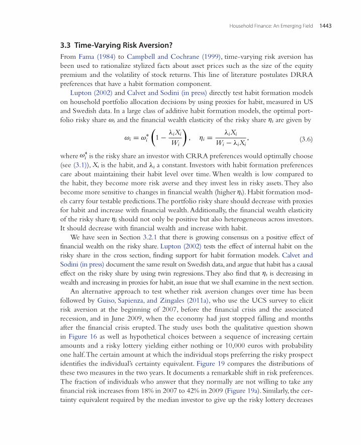
Household Finance: An Emerging Field 1443
3.3 Time-Varying Risk Aversion?From Fama (1984) to Campbell and Cochrane (1999), time-varying risk aversion has been used to rationalize stylized facts about asset prices such as the size of the equity premium and the volatility of stock returns. This line of literature postulates DRRA preferences that have a habit formation component.
Lupton (2002) and Calvet and Sodini (in press) directly test habit formation models on household portfolio allocation decisions by using proxies for habit, measured in US and Swedish data. In a large class of additive habit formation models, the optimal port-folio risky share ωi and the financial wealth elasticity of the risky share ηi are given by
where ω∗i is the risky share an investor with CRRA preferences would optimally choose
(see (3.1)), Xi is the habit, and λi a constant. Investors with habit formation preferences care about maintaining their habit level over time. When wealth is low compared to the habit, they become more risk averse and they invest less in risky assets. They also become more sensitive to changes in financial wealth (higher ηi). Habit formation mod-els carry four testable predictions. The portfolio risky share should decrease with proxies for habit and increase with financial wealth. Additionally, the financial wealth elasticity of the risky share ηi should not only be positive but also heterogeneous across investors. It should decrease with financial wealth and increase with habit.
We have seen in Section 3.2.1 that there is growing consensus on a positive effect of financial wealth on the risky share. Lupton (2002) tests the effect of internal habit on the risky share in the cross section, finding support for habit formation models. Calvet and Sodini (in press) document the same result on Swedish data, and argue that habit has a causal effect on the risky share by using twin regressions. They also find that ηi is decreasing in wealth and increasing in proxies for habit, an issue that we shall examine in the next section.
An alternative approach to test whether risk aversion changes over time has been followed by Guiso, Sapienza, and Zingales (2011a), who use the UCS survey to elicit risk aversion at the beginning of 2007, before the financial crisis and the associated recession, and in June 2009, when the economy had just stopped falling and months after the financial crisis erupted. The study uses both the qualitative question shown in Figure 16 as well as hypothetical choices between a sequence of increasing certain amounts and a risky lottery yielding either nothing or 10,000 euros with probability one half. The certain amount at which the individual stops preferring the risky prospect identifies the individual’s certainty equivalent. Figure 19 compares the distributions of these two measures in the two years. It documents a remarkable shift in risk preferences. The fraction of individuals who answer that they normally are not willing to take any financial risk increases from 18% in 2007 to 42% in 2009 (Figure 19a). Similarly, the cer-tainty equivalent required by the median investor to give up the risky lottery decreases
(3.6)ωi = ω∗i
(
1 −λiXi
Wi
)
, ηi =λiXi
Wi − λiXi,

Luigi Guiso and Paolo Sodini1444
from 4,000 euros in 2007 to 1,500 euros in 2009 (Figure 19b). Guiso, Sapienza, and Zingales (2011a) try to test various channels that could potentially explain these pat-terns. Though changes in these measures of risk aversion predict participation rates in the stock market, they do not correlate with changes in investor wealth, with measures of background risk, or with proxies for habit, measured in a variety of ways. They find instead that these changes are correlated with measures of knightian uncertainty and fear. This is consistent with evidence in neuro-economics and lab experiments that risk aversion is augmented by apprehension, anxiety and panic. Kuhnen and Knutson (2005) find that more activation in the anterior insula (the brain area where anticipatory nega-tive emotions are presumably located) is followed by increased risk aversion. Kuhnen and Knutson (2011) find that subjects exposed to visual cues inducing anxiety were subsequently more risk averse and less willing to invest in risky assets.
Evidence based on measures of risk aversion elicited over time indicates that investor financial decisions may not be captured by a model with habit alone. Especially in the face of extreme events like the 2007 recession, other time-varying factors related to fear may have played an important role. Results from the cross-section of household portfolio choices, even after controlling for a large set of observable and unobservable characteristics using twin regressions (Calvet and Sodini, in press), find instead support for habit forma-tion models and the role of wealth and habit in shaping household portfolio decisions.
2007
2007
2007
2007
2009
2009
2009 2009
0
10
20
30
40
50
60
Substantial risk and return
Above average risk and return
Average risk and return
No financial risk
% fr
eque
ncy
Figure 19a Risk Aversion and the Financial Crisis. Frequency distribution of a qualitative indicator of risk aversion obtained in the Italian 2007 UCS in the two years before and after the financial crisis.

Household Finance: An Emerging Field 1445
3.4 Heterogeneity in the Financial Wealth Elasticity of the Risky ShareThe empirical literature on household financial risk attitudes has mostly focused on the average investor and is largely silent on the possibility that risk preferences are hetero-geneous across households. As we discussed in Section 3.2.1, the sign of the estimated financial wealth elasticity of the risky share η gives us information on whether investors have decreasing, constant, or increasing relative risk aversion on average. We have seen that the average elasticity η is estimated positive in most studies. However this does not rule out the possibility that the elasticity is heterogeneous across investors and varies strongly with investor characteristics.
As we have seen in Section 3.3, habit formation models imply that the elasticity η is decreasing in wealth and increasing in habit. Wealthy investors with moderate habits behave very much like CRRA agents, whereas investors with high habits, compared to their means, are very risk averse and very sensitive to small changes in the habit to wealth ratio. Calvet and Sodini (in press) test these hypotheses using twin data and characterize how η varies with investor characteristics. Using a methodology similar to Ashenfelter and Rouse (1998), they estimate a specification of (3.4) in which the elasticity depends on the average characteristics of twin pairs ηp. In parametric and non-parametric regressions, they find that the elasticity is strongly decreasing with financial wealth. Figure 20 reports their findings on the relation between the financial wealth elasticity of the risky share and wealth. Poor households in the lowest quartile
20072007
2009
2009
0
500
1000
1500
2000
2500
3000
3500
4000
4500
Certainty equivalent amount:mean Certainty equivalent amount:median
Euro
Figure 19b Risk Aversion and the Financial Crisis. Mean and median certainty equivalent of a lottery paying 10,000 euros with probability ½ and 0 with the same probability, elicited in the sample of investors in the UCS in the two years before and after the financial crisis.
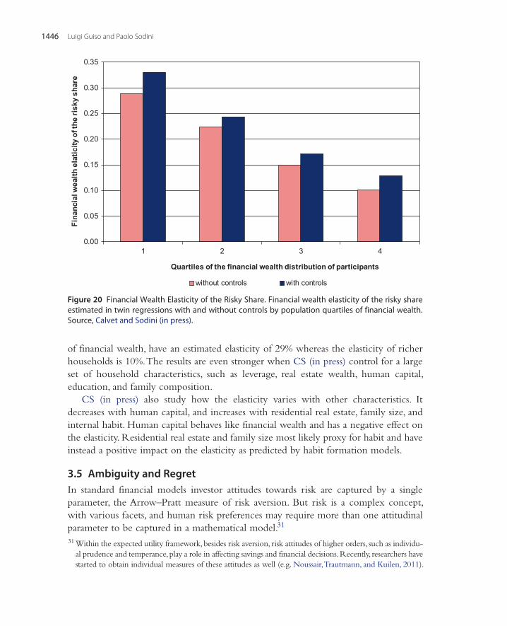
Luigi Guiso and Paolo Sodini1446
of financial wealth, have an estimated elasticity of 29% whereas the elasticity of richer households is 10%. The results are even stronger when CS (in press) control for a large set of household characteristics, such as leverage, real estate wealth, human capital, education, and family composition.
CS (in press) also study how the elasticity varies with other characteristics. It decreases with human capital, and increases with residential real estate, family size, and internal habit. Human capital behaves like financial wealth and has a negative effect on the elasticity. Residential real estate and family size most likely proxy for habit and have instead a positive impact on the elasticity as predicted by habit formation models.
3.5 Ambiguity and RegretIn standard financial models investor attitudes towards risk are captured by a single parameter, the Arrow–Pratt measure of risk aversion. But risk is a complex concept, with various facets, and human risk preferences may require more than one attitudinal parameter to be captured in a mathematical model.31
31 Within the expected utility framework, besides risk aversion, risk attitudes of higher orders, such as individu-al prudence and temperance, play a role in affecting savings and financial decisions. Recently, researchers have started to obtain individual measures of these attitudes as well (e.g. Noussair, Trautmann, and Kuilen, 2011).
0.00
0.05
0.10
0.15
0.20
0.25
0.30
0.35
1 2 3 4
Fina
ncia
l wea
lth e
latic
ity o
f the
risk
y sh
are
Quartiles of the financial wealth distribution of participants
without controls with controls
Figure 20 Financial Wealth Elasticity of the Risky Share. Financial wealth elasticity of the risky share estimated in twin regressions with and without controls by population quartiles of financial wealth. Source, Calvet and Sodini (in press).

Household Finance: An Emerging Field 1447
Two traits that researchers have considered are aversion to ambiguity and regret. These features can be embedded in (otherwise standard) expected utility models, com-bining them with preferences that also exhibit risk aversion in the Arrow-Pratt sense. The first trait originates from Ellsberg’s (1961) experiments which showed that indi-viduals tend to prefer a prospect with known probabilities to the same prospect with unknown probabilities. Returns on financial assets, particularly on securities that inves-tors are less familiar with or at times when prices provide unclear signals, are likely to provoke aversion to ambiguity and be considered uncertain in a knightian sense. Thus, aversion to ambiguity may potentially explain why investors demand a high equity premium to hold stocks (e.g. Epstein and Schneider, 2010).
The second trait, regret, is defined as the intelligent or emotional dislike an individual experiences after committing an action or making a decision that the person later wishes that he or she had not made. The anticipation of this feeling may influence individual choices. Financial investments offer many opportunities to regret. For example, after a crash, an investor may regret having heavily invested in the stock market. Anticipating this feeling, agents may become more reluctant to undertake risky investments. Of course, they may also regret missed gains, and thus in their choices they may end up balancing these two feelings. Insofar as the loss of a euro provokes more regret than the gain of it, regret may generate more prudent behavior.
Gollier (2006) studies whether ambiguity aversion amplifies risk aversion and a strand of the literature that we review in Sections 4.1 and 4.2, focus on the effect of ambiguity aversion on investor participation and portfolio composition. Few papers instead study the effect of regret. One exception is Gollier and Salanié (2006), who show that if expected utility maximizing investors are sensitive to regret, portfolio allo-cations are biased towards assets that perform particularly well in low probability states.
The empirical literature on the effects of these attitudes on household financial deci-sions is still at an early stage. To shed some light on household attitudes towards ambigu-ity and regret, Figure 21 shows the distribution of qualitative measures of attitudes towards uncertainty (panel A) and towards regret over gains and losses (panel B) in the UCS 2007 survey.32
Most individuals are averse to ambiguity (51.5%) and one third strongly so. One fourth are ambiguity neutral, i.e. indifferent between an ambiguous and a risky choice. Some (24%) seem to be ambiguity lovers. Many regret losses a lot (37.6%). The major-ity expresses some regret (42%) while 20% display no regret for past decisions. In the domain of missed gains, though the majority regrets, very few express major regret (9%) and a large fraction (42%) does not regret at all. Hence regret seems to be stronger for
32 See the notes to Figure 21 for the wording of the questions used to elicit ambiguity and regret preferences.

Luigi Guiso and Paolo Sodini1448
incurred losses than for forgone gains. Butler, Guiso, and Jappelli (2011) show that risk and ambiguity aversion tend to be correlated, because there is a common factor that drives them: the way individuals reach a decision. Those who rely mainly on intuition are readier to tolerate risk and ambiguity than deliberate thinkers. Observable charac-teristics affect these traits differently. While risk aversion is lower for males and young individuals, regret for losses is lower for males and, interestingly, declines with age. Aversion to ambiguity instead is not affected by gender or age. Most importantly per-haps, while risk aversion falls with wealth, regret and aversion to ambiguity are invariant to it. Insofar as regret and ambiguity matter for financial decisions, they may explain reluctance to take on risk even among the wealthier, at least in circumstances involving substantial uncertainty and the possibility to regret. The heterogeneity documented in Figure 21 may also help explain why investors hold different risky asset portfolios and choose different individual stocks. Unfortunately, empirical evidence on these issues is still lacking.
0
5
10
15
20
25
30
35
Strong preference forambiguous lottery
Preference forambiguous lottery
Indifferent Preference for riskylottery
Strong preference forrisky lottery
% fr
eque
ncy
Figure 21a Ambiguity Aversion. Frequency distribution of attitudes towards ambiguity in the 2007 UCS sample of investors. The ambiguity aversion index is obtained by facing participants with a choice similar to the one in Ellsberg (1961) asking: “Suppose you face two urns each with 100 balls. The first urn has 100 balls, some are red some are black and you do not know how many reds and how many blacks. The second urn has 100 balls, 50 red and 50 black. One ball is drawn from the urn that you choose and you will win 1000 Euros if the ball is of the color that you choose. Choose a color. Now tell me whether you prefer to have the ball drawn from the first or the second urn. Choose one of the following options, (1) A strong preference for the first urn; (2) A slight preference for the first urns; (3) Indifferent between the two urns; (4) A slight preference for the second urn; 5) A strong preference for the second urn.” A categorical variable between 1 and 5 identifies the five groups in increasing aversion to ambiguity.
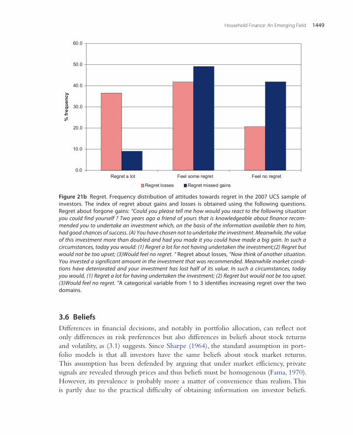
Household Finance: An Emerging Field 1449
3.6 BeliefsDifferences in financial decisions, and notably in portfolio allocation, can reflect not only differences in risk preferences but also differences in beliefs about stock returns and volatility, as (3.1) suggests. Since Sharpe (1964), the standard assumption in port-folio models is that all investors have the same beliefs about stock market returns. This assumption has been defended by arguing that under market efficiency, private signals are revealed through prices and thus beliefs must be homogenous (Fama, 1970). However, its prevalence is probably more a matter of convenience than realism. This is partly due to the practical difficulty of obtaining information on investor beliefs.
0.0
10.0
20.0
30.0
40.0
50.0
60.0
Regret a lot Feel some regret Feel no regret
% fr
eque
ncy
Regret losses Regret missed gains
Figure 21b Regret. Frequency distribution of attitudes towards regret in the 2007 UCS sample of investors. The index of regret about gains and losses is obtained using the following questions. Regret about forgone gains: “Could you please tell me how would you react to the following situation you could find yourself ? Two years ago a friend of yours that is knowledgeable about finance recom-mended you to undertake an investment which, on the basis of the information available then to him, had good chances of success. (A) You have chosen not to undertake the investment. Meanwhile, the value of this investment more than doubled and had you made it you could have made a big gain. In such a circumstances, today you would: (1) Regret a lot for not having undertaken the investment;(2) Regret but would not be too upset; (3)Would feel no regret. “ Regret about losses, “Now think of another situation. You invested a significant amount in the investment that was recommended. Meanwhile market condi-tions have deteriorated and your investment has lost half of its value. In such a circumstances, today you would, (1) Regret a lot for having undertaken the investment; (2) Regret but would not be too upset. (3)Would feel no regret. “A categorical variable from 1 to 3 identifies increasing regret over the two domains.

Luigi Guiso and Paolo Sodini1450
In recent years, however, reliable methodologies have been developed to elicit indi-vidual probability distributions of future events (see Guiso, Jappelli, and Terlizzese 1992, for an early application and Manski, 2004, for a review). Dominitz and Manski (in press) apply these methodologies to obtain probabilistic beliefs about stock market returns in a sample of US citizens. They find a tremendous amount of heterogeneity, not only in beliefs but also in the way individuals seem to form their beliefs. Hurd, Van Rooij, and Winter (2009) elicit probability distributions of stock market gains and losses in a sample of Dutch households and can thus compute not only mean expected stock returns but also higher moments. They find that investors not only have different opin-ions about mean returns but also about the variance of returns. In Table 4 we report the cross-sectional distribution of subjective risk free rates, expected stock returns and of assessed ranges (max-min) of possible return realizations in the 2007 UCS. On aver-age, Italian investors believe they can obtain 3.7% from a safe investment but at least 10% of them do not expect any return and the most optimistic 5% believe they will obtain a yield of at least 10% per year. The median expected stock return is 5.5% yearly but views are very dispersed, the investors in the 10th percentile expect to earn no returns while the one at the 90th percentile expects to make 24% over the same year. Uncertainty about stock returns, as measured by the subjectively assessed range of pos-sible return realizations, is equally dispersed. The mean range is 9.4%, roughly twice as much as the average return, but the 10th percentile is half of a percentage point and the 90th is 25%. It is interesting to note that those who hold higher expectations also hold them with higher uncertainty.
3.7 Risk Aversion, Beliefs, and Financial Choices; Putting Merton’s Model to the Test
The Merton model can be directly tested by using elicited measure of risk aversion and beliefs together with information on investors’ actual portfolio allocations. We construct empirical analogs of the variables in formula (3.1) by using risk aversion indicators and stock market beliefs elicited in the 2007 UCS survey.33 In the sample, the median investor believes in a risk free rate of 3% and an equity pre-mium of 2%.
Table 5 reports Tobit regressions of the risky share on risk aversion dummies, stock market beliefs, and total wealth. More risk averse investors hold significantly lower risky shares, and those who expect higher stock returns and perceive stocks as less risky, hold larger shares in risky assets. Not only are these effects qualita-tively consistent with the prediction of the standard Merton model but they are
33 See the caption of Table 5 for the definition of the variables.

Household Finance: An Emerging Field 1451
quantitatively important. The most risk tolerant investors have 49% more of their financial wealth invested in risky assets compared to the most risk averse. One per-centage point difference in the expected equity premium increases the risky share by eight percentage points. Adding wealth as a regressor, after controlling for belief and preference indicators, leaves the effect of the latter variables unchanged and results in a positive estimate of the wealth elasticity of the risky share. Since the average risky share in the sample is 26%, the wealth elasticity of the risky share is estimated at about 0.5.
The regression confirms the view that the elicitation of risk preferences and the revealed preference approach are both powerful and complementary methods to study household portfolio decisions in financial markets. Wealth strongly correlates with financial risk taking as measured by portfolio allocation in risky assets. One view is that the positive estimated coefficient might capture the effect of observable and unobserv-able characteristics left out from the regression. Another view is that it measures the causal effect of wealth, as argued in Section 3.2.1, providing support for DRRA risk preferences.
Table 4 Subjective Distribution of Stock Returns. Risk free rates, mean stock returns and range of stock returns obtained from subjective probability distributions elicited in the 2007 UCS. To elicit the risk free rate, investors were asked what would be the value of a 10,000 euro investment in a safe security after 12 months. To elicit beliefs about the stock market, investors were asked what would be the value of a 10,000 euro investment in a fully diversified stock mutual after 12 months. They were asked to report the minimum value and the maximum. Subsequently they were asked to report the probability that the value of the stock will be above the mid-point of the reported range by the end of the 12 months. Under the assumptions that the distribution is uniform, we have computed the subjective mean of stock market returns. The range of stock return is the difference between the maximum and minimum value of the investment Subjective distribution
Risk free rate Mean of stock return Range of stock return
Mean 1.037 1.066 0.094Standard deviation 0.045 0.196 0.129Percentiles 1 1 0.155 05 1 0.91 010 1 1 0.00525 1.02 1.024 0.0150 1.03 1.055 0.0575 1.04 1.115 0.190 1.06 1.24 0.2595 1.1 1.33 0.499 1.3 1.64 0.64

Luigi Guiso and Paolo Sodini1452
4. HOUSEHOLD PORTFOLIO DECISIONS, FROM NORMATIVE MODELS TO OBSERVED BEHAVIOR
One implication of the Merton model is that all investors, independently of their wealth and of their preferences towards risk, should participate in all risky assets mar-kets and should invest in the market portfolio.34 These implications fail in reality. Households do not behave as the basic theory predicts. A substantial fraction of house-holds do not participate in risky assets markets; those who do, do not hold the same securities and do not hold the market portfolio. There is a substantial discrepancy between the predicted homogeneity and the observed heterogeneity of household behavior.
In this section we first study the decision to participate in financial markets, the participation puzzle and the explanations that have been offered to resolve it. We then review the literature on how households decide to choose among risky financial assets. We study the level and determinants of diversification, the profitability and frequency
34 The market portfolio is the portfolio of all securities in the market with weights proportional to the securities’ market capitalizations.
Table 5 Share in Risky Assets. The table shows Tobit regressions of the portfolio risky share on total wealth, measures of elicited risk preferences, and dummies capturing measures of subjective beliefs about the stock market in the sample of investors surveyed in the 2007 UCS. The portfolio risky share is the fraction of total financial wealth invested in risky assets. The measures of risk preferences are derived from the ones used in Figure 16 omitting the dummy corresponding to the most risk averse group of investors. The measures of subjective beliefs are the ones used in Figure 4. The risk premium is obtained by subtracting the risk free rate from the mean stock return reported by each investor
(1) (2) (3)
Substantial risk and return 0.492*** 0.482*** 0.418*** (0.076) (0.076) (0.077)Above average risk and return 0.406*** 0.400*** 0.351*** (0.032) (0.032) (0.034)Average risk and return 0.275*** 0.267*** 0.226*** (0.030) (0.030) (0.031)Equity Premium 0.079*** 0.076*** (0.019) (0.020)Range of stock returns -0.129*** -0.117*** (0.040) (0.043)Log total wealth 0.134*** (0.022)Observations 1686 1686 1494Pseudo R2 0.0788 0.0866 0.0964

Household Finance: An Emerging Field 1453
of trading, and the delegation of portfolio decisions. We close the section by looking at portfolio rebalancing in response to market movements and over the life-cycle.
4.1 Stock Market ParticipationOver the past decade, a large literature, pioneered by Haliassos and Bertaut (1995), has been trying to explain the “participation puzzle”, i.e. why a substantial fraction of households do not invest in risky financial assets even though standard portfolio theo-ries, such as the basic Merton model of Section 3, imply that households should invest at least some wealth in risky assets to take advantage of the equity premium.
Figure 6 shows that only a fraction of US households participate in financial assets, particularly at low levels of wealth. In Table 6, we report participation rates across countries by quartiles of financial wealth. Limited stock market participation is not unique to the US and it is not restricted to direct stockholdings; it extends to a broad set of countries and to indirect ownership of public equity. Additionally, a pervasive feature of the data is that participation in stock markets is increasing with wealth and, strikingly, even at very high levels of wealth some households do not invest in equity. Finally, there are marked differences in average participations across countries. For example, very few hold stocks in Italy and even fewer in Spain, while, in the US or in Sweden, the median household is a stockholder. These differences are not merely a reflection of differences in GDP per capita. Italy, for instance, has a much lower stock market participation rate that the UK, but both countries have similar levels of per capita income.
A convincing explanation of the stockholding puzzle should be able to jointly account for all these features. Below we review some that have been offered in the litera-ture and look at explanations based on, transaction costs, non-standard preferences, and beliefs.35
4.1.1 Participation Costs and the Stockholding PuzzleHouseholds might decide not to invest in equity because they face fixed costs of partici-pation (Vissing-Jørgensen, 2003). Examples are varied and include monetary expenses (e.g. administrative charges to set up an investment account) and information costs (e.g. learning about financial products). Investors weight the fixed costs of participation against the benefit of investing in risky securities, which, in a rational model, is the risk premium
35 While we focus on these explanations, others have also been proposed. Following Merton (1987), Guiso and Jappelli (2005) argue that lack of awareness may explain why some (especially among the poor) do not invest in these assets. However their explanation cannot rationalize limited participation among the wealthy. Davis, Kubler, and Willen (2006) argue that the spread between borrowing and lending rates can explain why households do not invest in stocks. The positive correlation between labor income and stock market returns may, if sufficiently strong, discourage stockholding (Benzoni, Collin-Dufresne, and Goldstein, 2007). We discuss some of these explanations in greater detail in Section 4.4.3.

Luigi Guiso and Paolo Sodini1454
they can earn multiplied by the amount invested. Hence, fixed participation costs imply that more risk tolerant investors are more likely to participate because they are more likely to invest a larger share of their financial wealth in risky assets. The same is true for investors who face less background risk or who are less likely to be liquidity constrained. In general, any factor that increases the optimal portfolio risky share will encourage stock market participation. This can rationalize why stock market participation correlates with characteristics such as investor cognitive skills (e.g. Christelis, Jappelli, and Padula, 2010; Grinblatt, Keloharju and Linnainmaa, 2011), financial literacy and education (Cole and Shastry, 2009; Van Rooij, Lusardi, and Alessie, 2007), and risk aversion (Guiso and Paiella, 2006; Haliassos and Bertaut, 1995). Most importantly, fixed participation costs are consistent with the strong positive correlation between participation and wealth, as documented in Table 6.
Since participation costs are not observables, a test of the theory rests partly on its implications and partly on the estimates of the size of these costs. Direct estimates are hard to obtain. One could use information on trading and holding fees, but these are not necessarily fixed and paid upon entry, and in addition they can only provide a lower bound to the estimated costs of participation. Alternatively, one could follow a revealed preference approach and infer participation costs from observed behavior (Attanasio and Paiella, 2011; Calvet, Campbell, and Sodini 2007a; Luttmer, 1999; Paiella, 2007; Vissing-Jørgensen, 2003). The estimates found in the literature with the revealed preference approach are sufficiently small to be reasonable, thus making the participation cost explanation plausible. Additionally, the increase in stock market participation that has taken place over the past two decades is also consistent with a decline in participation costs. The availability of financial information on the Internet, and the expansion of the mutual fund industry have effectively made access to the equity market cheaper.
However, there are features of the data that are hard to reconcile with the fixed participation story. First, it is hard to explain the marked cross-country differences in stockholdings, particularly when one compares countries at similar level of economic and financial development such as Sweden and Germany. Second, it is difficult to rationalize with (small) participation costs the lack of participation at high levels of wealth is many countries. For instance, Table 6 reports that, even among the top 5% wealthiest investors, 28% have no stocks in the Netherlands, 39% in Germany, and 75% in Spain.
4.1.2 Non-Standard Preferences and Limited Stock Market ParticipationAn alternative route that has been followed to explain the participation puzzle is to consider non-standard preferences. For instance, Barberis, Huang, and Thaler (2006) show that individuals with loss aversion preferences and narrowly framed portfolio decisions choose to stay out of the stock market even without direct participation costs.

Household Finance: An Emerging Field 1455
This explanation is consistent with Dimmock and Kouwenberg (2010), who find that an elicited measure of loss aversion is correlated with the probability of investing directly or indirectly in stocks.
Similarly, if stock returns are ambiguous and investors are averse to ambiguity, it may be optimal not to participate altogether in the stock market, as long shown by Dow and Werlang (1992) in the context of a two assets portfolio model with one ambiguous and
Table 6 Proportion of households investing in stocks. The first panel shows the proportion of households who owns directly stock in each quartile of gross financial wealth. The second panel shows the same proportion when we include also indirect ownership, via mutual funds or pension funds. Data for European countries is computed from the 2004 wave of the Survey for Health, Age, and Retirement in Europe (Share), and refer to year 2003. Data for the US is drawn from the 1998 Survey of Consumer Finances. Data for the UK is drawn from the 1997 to 1998 Financial Research SurveyA. Direct Stockholding
Quartile I Quartile II Quartile III Quartile IV Top 5 % Average
US 1.4 6.9 20.6 47.9 70.1 19.2UK 0 4.4 28.3 53.6 67.9 21.6Netherlands 1.5 7.4 20 40.3 60.2 17.2Germany 0.6 4.1 16.1 36.1 50.5 14Italy 0 0.8 3.1 12.8 30.8 4Austria 0 1.7 2.8 15.6 25.7 5Sweden 12.9 30.7 46.9 72.8 80.6 40.8Spain 0 0.3 1.8 13.2 14.4 3.5France 0.7 9.9 14.6 33.3 44.2 14.4Denmark 6.3 25.9 36.4 55.6 68.4 31Greece 0 0.7 3.2 17.3 23.5 4.9Switzerland 2.8 12.2 30.3 54.2 63.2 24.9
B. Direct and Indirect Stockholding
Quartile I Quartile II Quartile III Quartile IV Top 5 % Average
US 4.4 38.3 66 86.7 93.7 48.9UK 4.9 11.9 37.8 71.1 83.9 31.5Netherlands 1.7 11 31.3 52.8 72 24.1Germany 1.5 11.8 28.7 51.4 61.2 22.9Italy 0 0.8 5.2 27.5 64.8 8.2Austria 0 1.9 8.1 25.5 33.8 8.8Sweden 25.8 63.4 82.7 92.9 95.8 66.2Spain 0 1.1 3 19.1 24.6 5.4France 1.1 17.6 29.9 57.6 67.3 26.2Denmark 6.6 30.8 44.8 65.7 75.4 37Greece 0 0.7 4 22.2 32.9 6.3Switzerland 2.8 20 38.2 63.7 65.8 31.4

Luigi Guiso and Paolo Sodini1456
one unambiguous asset, and, more recently, by Garlappi, Uppal, and Wang (2007) in a model with multiple ambiguous assets (see Epstein and Schneider, 2010, for a review).
While the combination of loss aversion, narrow framing, and ambiguity can potentially rationalize why some households do not participate, it is unlikely to explain the positive correlation between participation and wealth, the lack of par-ticipation at high wealth levels, and the persistent cross-country differences in stock market participation. One would have to make assumptions about how loss aversion, narrow framing, and ambiguity affect individuals at different levels of wealth and, if one were to rely on preference-based explanations, why they differ systematically across populations in a way that can explain the observed differences in stock market participation.
4.1.3 Beliefs and Stock Market ParticipationIn portfolio theory with standard expected utility preferences, investors hold risky assets to earn the risk premium. If individuals believe that the stock market does not yield an expected return in excess of the risk free rate, they will choose to stay out of the mar-ket, even in the absence of participation costs. Hurd, Van Rooij, and Winter (2009) and Kezdi and Willis (2009) use information on elicited beliefs about stock market returns for Dutch and American investors, respectively, and find that those with more optimis-tic beliefs about stock returns are more likely to participate. The results in Table 4 are also consistent with the idea that individuals with low expectations about stock market returns choose to stay out of the market. These estimates also show another dimension of beliefs that reinforces limited participation, the riskiness about stock market returns as measured by the perceived return volatility. Though in itself a high level of uncertainty about the stock market would not be able to explain non-participation within Merton’s framework, perceived riskiness can greatly amplify the effect of small per-period costs of participation.
In the Merton-type model, the share invested in risky assets depends on their Sharpe ratio, i.e. the equity premium per unit of risk taken Ere
i /σi. Coupled with fixed par-ticipation costs and investor home bias, variations in Sharpe ratios across countries may also contribute to explain cross countries differences in participation. To explore this possibility, Dimson, Marsh, and Staunton (2002) collect stock market performance dur-ing the 20th century for several countries. While investors earn an equity premium in all countries, there is dispersion in its size and in stock market volatility, which translates in differences in the Sharpe ratio.
The data in Dimson, Marsh, and Staunton (2002) seem to suggest that indeed stock market participation is lower in countries with higher stock market volatility and is higher in countries with higher Sharpe ratio. Needless to say, the high volatility may be a reflection of stock market thinness due to limited participation rather than its cause.

Household Finance: An Emerging Field 1457
The perceived Sharpe ratio depends also on the portfolio diversification an investor is able to achieve. As we will see in Section 4.2.1, Calvet, Campbell, and Sodini (CCS, 2007a) show that less sophisticated households tend to hold less diversified portfolios. The typical non-participating household, being poorer and uneducated, would invest in a poorly diversified portfolio if it were to participate, thus earning a lower risk premium. CCS (2007a,b) show that this effect reduces the estimates of participation costs by half to two-thirds compared to those obtained previously in the literature. Households that are aware of their limitations need substantially lower participation costs to stay out of the market.
While the decision to participate requires investors to form beliefs about the risk-return trade-off achievable by investing in risky assets, it also requires confidence in information sources, financial advisors, portfolio managers, and, more generally, on the overall reliability of the financial system. Guiso, Sapienza, and Zingales (GSZ, 2008) focus on the role of trust in driving individual willingness to participate in the stock market. They argue that many individuals may perceive the stock market as a three-card game played on the street. Even after observing many rounds, they may not trust the fairness of the game (and the persons playing it). Episodes such as the Enron bankruptcy or the Madoff scandal, may not only change subjective probabilities about asset returns, but the fundamental trust in the system that delivers those payoffs. GSZ (2008) develop a model showing that wary investors might not participate since their lack of trust dissolves the perceived risk premium. Trust reflects the objective characteristics of the financial system (the quality of investor protection, its enforcement, etc.) but also inves-tor beliefs and backgrounds. Differences in social norms rooted in past history (Guiso, Sapienza, and Zingales, 2004) or in religious upbringing (Guiso, Sapienza, and Zingales, 2003) can create considerable differences in levels of trust across individuals, regions, and countries. To assess the power of a trust-based explanation they rely on a Dutch survey with information on attitudes towards trusting other individuals. They find that trust indeed predicts investor stockholding decisions and that the result is robust to the inclu-sion of controls for individual risk and ambiguity aversion. They conclude that trust and preferences for risk play different roles in the participation decision. Additionally, the effect of trust cannot be due to unobservable institutional differences since all investors are drawn from the same country.
There are three important implications of the trust-based explanation. First, since trust is a (relatively) stable individual trait, it can explain the persistent reluctance or inclination to invest in risky assets (Calvet, Campbell, and Sodini 2009a). Second, since trust does not vary much across wealth levels, it can explain limited participation even among the wealthy. Furthermore, even though participation costs are still needed to explain the difference in participation between the wealthy and the poor, lack of trust amplifies the effect of costly participation. For example, if an investor thinks that there is a 2% probability of being cheated, the threshold level of wealth beyond which he invests
Luigi Guiso and Paolo Sodini1458
in the stock market can increase by a factor of five (GSZ, 2008). Third, as illustrated in Figure 22, since trust varies systematically across nations, as differences in trust are deeply rooted in popular culture, it can help explain differences in participation across countries (GSZ, 2004, and Georgarakos and Pasini, 2009).
4.1.4 Limited Participation in Other Financial InstrumentsLimited participation is a broader phenomenon that involves not only risky financial securities. Not all households hold debt (see Figure 13) and many do not participate in insurance markets. Some of the forces that lead households to stay out of risky securities may be also advocated to explain lack of participation in insurance or in debt market. For instance, bankruptcy costs may discourage borrowing and, with unfair insurance pricing, risk tolerant individuals may decide not to insure leaving the mar-ket to the more risk-averse (Mossin, 1968). Guiso (2010) documents the role of trust, and finds that small business owners buy broader coverage insurance contracts if they trust insurance companies more. In an experiment involving true insurance sellers, De Meza, Irlenbusch, and Reyniers (2011) find that more trusting subjects are willing to
Australia
Austria
Switzerland
Germany
Denmark
Finland
France
Japan
Greece
India
Ireland
Italy
United Kingdom
Sri Lanka
Netherlands
Norway
New Zeland
Portugal
Singapure
Sweden
Thailand
Turkey
United States
-
0.05
0.10
0.15
0.20
0.25
0.30
0.35
0.40
0.45
- 0.10 0.20 0.30 0.40 0.50 0.60 0.70Trust
PARTICIPATION Fitted values
Belgium
Figure 22 Trust and stock market participation across countries. The figure plots direct stock market participation against the average level of trust (from the World Values Survey. Source, Guiso, Sapienza, and Zingales, 2008).

Household Finance: An Emerging Field 1459
pay larger insurance premium to sellers that advertize the policy. They interpret the finding as suggesting that trusting individuals are easier to persuade about the quali-ties of the insurance product. In an interesting paper that relies on a field experiment in Indian villages, Cole et al. (in press) document that peasant adoption of insurance contracts significantly increases when the products are endorsed by a reputable person in the village.
4.1.5 The Bottom Line on Participation PuzzlesThe literature on the participation puzzle is the oldest in household finance and is large. Compared to other areas, it provides us with well-established stylized facts that are diffi-cult to reconcile with standard portfolio choice theory. Participation costs, non-standard preferences, and belief heterogeneity, not only in the form of subjective probabilities about future returns but also in terms of trust, capture different features of the data and probably each of them contributes to the explanation of the non-participation phe-nomenon. The challenge for future research is to identify when and for which investors some of the explanations are more relevant than others. Participation has been studied mostly in a static framework, and the decision to enter and exit risky financial markets has received relatively little attention, probably because many datasets lack the desirable panel structure. We refer the reader to Sections 4.3 and 4.4.6 for a review of the thin literature on entry and exit decisions.
4.2 Portfolio SelectionOnce households decide to participate in risky asset markets, they are faced with a number of decisions: how much to invest in risky assets, which assets to buy, whether to invest through a fund manager, and whether to follow the recommendations of a financial advisor.
In Section 3 we have reviewed the literature on how households decide on the proportion of financial wealth invested in risky assets. We have seen how the portfolio risky share depends on financial wealth, background risk, demographic characteristics, personality traits and intelligence, beliefs, and non-standard preferences. In this section we focus on the composition of the portfolio risky share. Do households hold diversi-fied portfolios? Which assets do they decide to buy? How do they trade? Do they invest through a fund manager or directly? Do they rely on financial advisors and follow their recommendations?36
36 In this chapter, we abstract from the impact of taxes on investment and trading decisions such as investment in tax deferred accounts or realization of capital losses for tax optimization purposes (Constantinides and Scholes, 1980; Constantinides, 1983; Poterba, Venti, and Wise, 1994; Poterba, 2001; Poterba and Samwick, 2003).
Luigi Guiso and Paolo Sodini1460
4.2.1 DiversificationOne of the basic precepts of financial theory is to hold a diversified portfolio, i.e. to avoid concentrating risk in one or few (possibly correlated) assets (Markowitz, 1952). Do households follow this simple and basic principle of financial theory? If they do, how do they achieve diversification? If they do not, how heterogeneous are household portfolios? How large and costly is under-diversification? Which households are more diversified?
These basic questions can only be answered by using reliable, highly detailed, and comprehensive information on the portfolio holdings of a representative sample of the population. Unfortunately, datasets that satisfy these requirements are rare. Surveys contain information on a representative sample of the population but cannot be too detailed and are sometimes imprecise since households, especially the wealthy, do not like to share information on their finances. Information on individual accounts held at brokerage houses (e.g. Odean, 1998, 1999; Schlarbaum, Lewellen, and Lease, 1978) is very accurate and detailed but it is limited to the clients of the brokerage house, which is a highly selected sample of investors, and to the assets held at the broker-age house, which might not be representative of total financial wealth. Similar issues arise with data based on 401(k) accounts and other tax-favored retirement accounts (Agnew, Balduzzi, and Sunden, 2003; Benartzi and Thaler, 2001; Choi et al. 2002, 2004; Madrian and Shea, 2001). Researchers have used registers of ownerships (e.g. Grinblatt and Keloharju, 2001a, and Massa and Simonov, 2006) to obtain accurate and detailed data for a representative sample of the population, but the information is limited to directly held stocks and does not consider holdings of mutual funds and other risky assets.
These data limitations have hampered research on the level of diversification in household financial portfolios. In a pioneering work, Blume and Friend (1975, 1978) use 1971 tax records and the 1962 Federal Survey of the Financial Characteristics of Consumers to obtain measures of risky portfolio composition for a representative sample of the population. Since the data provides only incomplete information on mutual fund holdings, they proxy diversification with the number of directly held stocks and the sum of squared shares held directly in stocks.37 They find that a large fraction of households hold undiversified portfolios of directly held stocks, more than 50% of stockowners have no more than two stocks. Their analysis builds on the Evans and Archer (1968) result that about ten stocks are needed to achieve a diversified portfolio, but does not take into account that a high level of diversification can be achieved by investing in a very limited number of mutual funds. Subsequent work by Kelly (1995)
37 When the market capitalization share of each stock in the market portfolio is small, this measure is approximately the sum of the squared deviations of the shares invested in each stock from stock shares in the market portfolio.
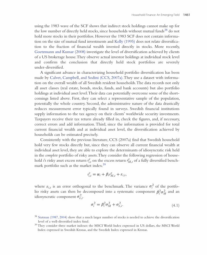
Household Finance: An Emerging Field 1461
using the 1983 wave of the SCF shows that indirect stock holdings cannot make up for the low number of directly held stocks, since households without mutual funds38 do not hold more stocks in their portfolios. However the 1983 SCF does not contain informa-tion on the size of mutual fund investments and Kelly (1995) does not relate diversifica-tion to the fraction of financial wealth invested directly in stocks. More recently, Goetzmann and Kumar (2008) investigate the level of diversification achieved by clients of a US brokerage house. They observe actual investor holdings at individual stock level and confirm the conclusion that directly held stock portfolios are severely under-diversified.
A significant advance in characterizing household portfolio diversification has been made by Calvet, Campbell, and Sodini (CCS, 2007a). They use a dataset with informa-tion on the overall wealth of all Swedish resident households. The data records not only all asset classes (real estate, bonds, stocks, funds, and bank accounts) but also portfolio holdings at individual asset level. Their data can potentially overcome some of the short-comings listed above. First, they can select a representative sample of the population, potentially the whole country. Second, the administrative nature of the data drastically reduces measurement error typically found in surveys. Swedish financial institutions supply information to the tax agency on their clients’ worldwide security investments. Taxpayers receive their tax return already filled in, check the figures, and, if necessary, correct errors and add information. Third, since the information is provided for total current financial wealth and at individual asset level, the diversification achieved by households can be estimated precisely.
Consistently with the previous literature, CCS (2007a) find that Swedish household hold very few stocks directly but, since they can observe all current financial wealth at individual asset level, they are able to explore the determinants of idiosyncratic risk held in the complete portfolio of risky assets. They consider the following regression of house-hold i’s risky asset excess return re
i,t on the excess return reM ,t of a fully diversified bench-
mark portfolio such as the market index.39
where εi,t is an error orthogonal to the benchmark. The variance σ 2i of the portfo-
lio risky assets can then be decomposed into a systematic component β2i σ 2
M and an
idiosyncratic component σ 2ε,i.
38 Statman (1987, 2004) show that a much larger number of stocks is needed to achieve the diversification level of a well-diversified index fund.
39 They consider three market indexes: the MSCI World Index expressed in US dollars, the MSCI World Index expressed in Swedish Kronas, and the Swedish Index expressed in Kronas.
rei,t = αi + βi r
eM ,t + εi,t ,
(4.1)σ 2i = β2
i σ 2M + σ 2
ε,i.
Luigi Guiso and Paolo Sodini1462
According to the CAPM, the household portfolio expected return is proportional to the expected return on the market.
i.e. households are compensated only for taking systematic risk. The CAPM implies that idiosyncratic risk increases the volatility of household portfolios without improving their expected return. In order to hold only systematic risk and maximize the portfo-lio Sharpe ratio, E re
i,t/σi, households have to be fully diversified and hold the market portfolio.
CCS (2007a) find that households with high idiosyncratic risk have concentrated portfolios in individual stocks, whereas households with low idiosyncratic risk have concentrated portfolios of mutual funds. In the middle of the idiosyncratic risk distri-bution, there are households with portfolios of mutual funds and stocks that tend to be more correlated with one another. Diversification is then sought through holdings of mutual funds and not by individual stock ownership. A good proxy for diversification is not the number of directly held stocks but the share of risky assets invested in funds. In the Swedish data, the correlation with the portfolio Sharpe ratio is only 6% for the first measure and climbs to 62% for the second (Calvet, Campbell, and Sodini, 2009b).
Losses from under-diversification are potentially severe for households that hold a large fraction of financial wealth in risky assets. When most wealth is held in safe assets, a concentrated portfolio in stocks has very little impact on household welfare. CCS (2007a) show that the majority of Swedish households suffer only modest losses from idiosyncratic portfolio risk. Households with more idiosyncratic risk invest a lower frac-tion of wealth in risky assets thereby reducing losses from under-diversification. As Kelly (1995) found, there are agents that hold only few stocks in their portfolio and carry high idiosyncratic risk, however these agents limit their losses by investing little in risky assets. Figure 23 illustrates this finding using the decomposition (4.1) implemented in CCS (2007a,b) with data from the 2007 Swedish Wealth Registry. On the horizontal axis, we consider bins of the risky share in 5% increments. On the vertical axis, we report the average annualized idiosyncratic risk σǫ,i of the households in the corre-sponding bin.40 Idiosyncratic risk is higher than 20% only for those households that invest less than 10% of their financial wealth on risky assets. It drops quickly and remains basically below 16% for households with a risky share larger than 25%. The relationship is slightly u-shaped. Households with most of their financial wealth invested in risky assets are richer (as we saw in Section 3) and may hold individual stocks for incentive reasons or because they possess (or believe they possess) superior information. In Section 4.2.2 we study the role of information in explaining under-diversification in household portfolios.
Erei,t = βiEre
M ,t ,
40 As in CCS (2007a, 2007b), we use the MSCI world index expressed in US dollars as benchmark in (4.1).
Household Finance: An Emerging Field 1463
CCS (2007a) find that, even though households display significant heterogeneity in their portfolio choices, the median household loses only 30 basis points of financial wealth, and 90 basis points of its risky financial assets per year, when benchmarked on the world index expressed in local currency.41 For a minority of households, however, losses from under-diversification are substantial, 5% of households lose over 5% in aver-age portfolio return or $850 per year (more than 3% of their disposable income).
Diversification losses and sophistication are tightly connected. CCS (2007a) finds that poorer, less educated households tend to invest inefficiently, earning only a small reward for the risk they take. Sophistication is also correlated with risk taking. Poorer and uneducated households take less risk, thereby reducing the losses caused by the larger idiosyncratic risk they have in their portfolio. These findings lead to the intriguing interpretation that households might be, at least partially, aware of their limited capabili-ties when they decide how much risk to take. Using US data, Polkovnichenko (2005) argues that households understand the consequences of being exposed to idiosyncratic risk. He shows that, among the respondents in the SCF survey that hold stocks directly, those with higher education invest a lower proportion of financial wealth in directly held stocks and in risky assets. Guiso and Jappelli (2008) are able to study the effect of financial literacy on portfolio diversification directly. Their data provides measures of financial literacy obtained with standard survey questions used in the financial literacy literature (Lusardi and Mitchell, 2007; Lusardi, 2008). Additionally, their data has admin-istrative information on the fraction of total financial wealth invested in equity through mutual funds, the direct investment in stocks and the number of stocks held in the portfolio. They use this information to construct an accurate and comprehensive mea-sure of portfolio diversification as suggested in Calvet, Campbell, and Sodini (2009b).42 They find that financial literacy is strongly correlated with portfolio diversification, but it is only weakly correlated with self-assessed financial competence.
Diversification is one of the basic principles of optimal portfolio selection. It is cheap to obtain and the lack of it can be extremely costly. It is challenging to measure diversifi-cation in household portfolios since one needs very detailed information on all security holdings. In Sweden such information is available, and most Swedish households avoid significant losses from under-diversification by holding mutual funds, and by reduc-ing risk exposure when they take idiosyncratic risk. Better educated, richer, and more financially literate households have better diversified portfolios. However, a minority of households suffer large losses from under-diversification. In the next section, we study
41 The median household loses 1.17% of its financial wealth and 2.92% of its investment in risky assets, when evaluated against the MSCI world index expressed in USD. These estimates are the appropriate ones if one believes that Swedish households should be able to efficiently hedge against currency fluc-tuations.
42 See Calvet, Campbell, and Sodini (2009c) for a detailed description of the methodology and for an evaluation of various proxies of portfolio diversification.

Luigi Guiso and Paolo Sodini1464
theories of under-diversification and review the empirical evidence on why households might want to be under-diversified.
4.2.2 Under-Diversification, Information, Hedging, and PreferencesThe fact that more sophisticated households are better diversified can be interpreted as evidence that under-diversification is the result of mistakes, i.e. households would choose to invest in diversified portfolios if they were told of the negative consequences of being under-diversified. This view is taken by Calvet, Campbell, and Sodini (2009b) who show that an index of financial sophistication, constructed from household char-acteristics, can jointly explain a set of three investment mistakes.
Another possibility is that deviations from diversified portfolios are the result of a rational choice or are induced by systematic behavioral biases. Theories of under-diversification can be divided into three broad categories. First, investors might hold portfolios that differ from the market when they do not have the same information or when some assets are more difficult to evaluate than others. Second, investors might simply have a taste for certain financial asset characteristics, such as proximity, or might
0.1
0.12
0.14
0.16
0.18
0.2
0.22
0.24
0.05 0.1 0.15 0.2 0.25 0.3 0.35 0.4 0.45 0.5 0.55 0.6 0.65 0.7 0.75 0.8 0.85 0.9 0.95
Idio
sync
ratic
risk
Risky share
Figure 23 Diversification and Risk Taking. Average idiosyncratic risk of the risky portfolio by bins of the share of financial wealth invested in risky assets. Participating households among 100,000 ran-domly selected households in the 2007 Swedish Wealth Registry.

Household Finance: An Emerging Field 1465
display non-standard preferences, such as prospect theory, that induce them to take on idiosyncratic risk. Third, individual portfolio heterogeneity can be driven by the need to hedge endowment risk such as income risk or risk connected to the investor geographi-cal location. In this section we first review existing rational and behavioral theories of under-diversification and then we report the empirical evidence available on why households decide to hold under-diversified portfolios.
Information. Like non-participation, under-diversification can simply be the result of households facing fixed learning or transaction costs (Brennan, 1975), that limit awareness of available investment opportunities. Merton (1987) studies an economy where investors have the same information on the securities they jointly know about, but each investor is aware only about a subset of the available securities. He shows that in equilibrium, the market portfolio is not mean-variance efficient and investors’ port-folio shares are different from the market portfolio. Uppal and Wang (2003) propose a model with ambiguity averse agents in which some assets are more difficult to value than others, and investors are averse to the possibility of model misspecification. UW (2003) calibrate their model to international equity markets and show that even small differences in ambiguity might induce investors to optimally choose severely under-diversified portfolios.
Van Nieuwerburgh and Veldkamp (2009) consider an equilibrium model with endogenous information acquisition. In equilibrium, investors optimally take larger positions in the assets they learn about than standard theory dictates. Optimal portfolios have two components: a fully diversified portfolio plus a learning portfolio, consisting of assets investors acquire information on. The learning portfolio can be specialized in one asset, or spread among multiple assets depending on the form of investor’s prefer-ences. Van Nieuwerburgh and Veldkamp (2010) show that investors rationally choose to specialize and take larger positions on assets in which they have a prior informational advantage since these assets offer, in equilibrium, higher risk-adjusted returns. According to their theory, if informational advantage reflects observations from the local environ-ment, investors decide optimally to tilt their portfolios towards local or professionally close stocks and will earn higher risk-adjusted returns as a consequence.
Preferences. Theories of under-diversification based on preferences argue that inves-tors prefer certain financial assets regardless of their payoffs. Huberman (2001) argues that investors have a taste for familiar assets whether or not they represent a profitable investment. Familiarity can take many forms, such as professional or geographical prox-imity, and it stems from preference inclinations, not from informational advantage. A preference for the familiar can also be the reflection of ambiguity averse preferences an idea made precise in Boyle, Uppal, and Wang (2010).
Mitton and Vorkink (2007), Barberis and Huang (2008), and Polkovnichenko (2005) consider investors that have a taste for positively skewed payoffs, for example because they have prospect theory preferences. Fama and French (2007) study the

Luigi Guiso and Paolo Sodini1466
equilibrium of an economy in which some investors value financial assets as consump-tion goods and choose them simply because they like them. In their model the market portfolio is not mean-variance efficient and investors hold undiversified portfolios in equilibrium. Interestingly, even investors who do not view securities as consump-tion products, and value them only based on their payoff, are under-diversified in equilibrium, since they have to hold the residual supply of assets. Roussanov (2010) adds another channel through which preferences might affect diversification. Investors concerned about social status hold idiosyncratic risk to increase their chances to “get ahead of the Joneses”.
Hedging. Investors are endowed with their own individual risk. They hold jobs, own houses, run businesses, live in specific locations, and have different educations. To the extent that their endowment risk is correlated with financial securities, investors should tilt their portfolios away from the market in order to reduce their exposure to those assets that are correlated with their own endowment risk (Calvet, Gonzales-Eiras and Sodini, 2004; Cochrane, 2008; Davis and Willen, 2000; Duffie et al. 1997). In this way they will reduce their overall, financial and non-financial, risk exposure compared to the case in which they hold the market portfolio. In partial equilibrium, there is a clear ten-sion between hedging needs and the prediction of models with differential information and familiarity. For example, on the one hand investors should shy away from stocks of sectors close to their professional expertise since they are likely to be correlated with their human capital. On the other, investors might decide to hold professionally close stocks since they are more likely to have superior information about them or feel them as familiar. In general equilibrium, however, limited resources might induce agents to rationally invest in assets positively correlated with their own endowment risk in order to hedge their relative wealth in the local community (DeMarzo, Kaniel, and Kremer, 2004). Prices of local goods and services in limited supply have prices that are increasing in aggregate wealth, hence financial assets whose payoffs are correlated with total wealth are highly valuable to local investors.
Empirical Evidence. Theories of under-diversification are difficult to test since they require very detailed and comprehensive data on both household portfolio composi-tion and household characteristics. Most of the empirical literature has focused on individual stockholdings to distinguish among possible causes of under-diversification. A growing, but still thin, literature sheds light on the relation between the level of diversification households achieve in their portfolios and why households choose to hold idiosyncratic risk.
It is widely established that investors tend to buy familiar stocks. Barber and Odean (2008) finds that individual investors buy attention-grabbing stocks, such as those of firms that appear prominently in the news, more than they sell them. He also shows that institutional investors are free of the same bias. Grinblatt and Keloharju (2001a) docu-ment that Finnish investors are more likely to hold, buy, and sell stocks of firms that are

Household Finance: An Emerging Field 1467
located close to the investor, that communicate in the investor’s native tongue, and that have a chief executive of the same cultural background.
A large literature establishes that professional money managers and traders have a tendency to buy local stocks and, by doing so, are able to earn positive abnormal returns (Choe, Kho, and Stulz, 1999; Coval and Moskowitz, 1999, 2001; Dvorak, 2005; Hau, 2001a). It is instead unclear whether individual investors have superior informa-tion about the familiar stocks they buy. Early findings indicate that individual investors earn abnormal returns from buying geographically and professionally close stocks and thus seem to react on information (Ivkovic, Sialm, and Weisbenner, 2008; Ivkovic and Weisbenner, 2005; Massa and Simonov, 2006). More recently, Døskeland and Hvide (2011) find the opposite result on Norwegian data. They provide evidence that profes-sional investment bias results in negative risk adjusted returns, and argue that investors suffer from overconfidence. Similarly, Seasholes and Zhu (2010) show that portfolios based on local holdings of the clients of a US brokerage house do not generate abnor-mal performance.
Keloharju, Knupfer, and Linnainmaa (2012) look at customer relationships and cus-tomer loyalty (Cohen, 2009). They find that Finnish customers are more likely to buy and less likely to sell the stocks of the products they purchase and the services they use, with a stronger bias for investors with a longer customer relationship. They argue that these facts cannot be simply explained by Merton’s notion of security awareness, since they are present not only for buying decisions but also when investors sell assets in their portfolios. KKL (2012) lean towards a preference-based explanation rather than one based on information and beliefs. Their findings support the Fama and French (2007) theory that financial assets are considered by many investors as any other consumption good. Evidence of limited investor awareness is instead provided by Guiso and Jappelli (2005), who find that awareness of financial securities correlates with education, house-hold resources, long-term bank relations, and proxies for social interactions.
When investors move away from the market portfolio, they hold familiar stocks, stocks that capture their attention or are connected to products they consume. Some authors suggest that these investment decisions are driven by awareness and informa-tion, others point to explanations based on preferences, and behavioral traits. In any case, direct stock investment is only a part of household financial wealth and the same person might be investing in more than one stock at the same time. How do individual stock investment decisions relate to the overall household financial wealth?
Two papers based on US brokerage account data relate individual stock invest-ment decisions with the rest of the portfolio directly held in stocks. Ivkovic´, Sialm, and Weisbenner (2008) show that investors with more concentrated stock portfolios achieve better performance especially on local stocks and on stocks not in the S&P 500. Goetzmann and Kumar (2008) instead find that equity portfolio concentration is not profitable and it is costly for most but a minority of investors who are persistently

Luigi Guiso and Paolo Sodini1468
able to exploit superior information. Investors concentrate their directly held equity portfolios in stocks with high volatility and high skewness.
As already mentioned in 4.2.1, Calvet, Campbell, and Sodini (2007a) argue that investors with high idiosyncratic risk in their directly held stock portfolio tend to reduce their under-diversification losses by investing most of their financial wealth in mutual funds and/or by limiting their risk exposure altogether. This interpretation receives further support by Anderson (2011) who merges trading data from a Swedish brokerage house with the Swedish Wealth Registry. He is able to observe the fraction of total risky financial wealth, or “stake”, the investors have in stocks at the brokerage house. Even among the skewed sample of brokerage house clients, many have a small stake, 20% of the sample has a stake of less than 5%, the median investor less than 35% and only 30% of the investors have a stake of more than 75%. In other words, it seems that most households choose to expose only a small fraction of the wealth invested in risky assets to frequent trading. This suggests that drawing general conclusions from investment behavior of brokerage house clients can be problematic, and that there is clearly a wide dispersion of how much the stock investment choices highlighted in the literature can affect investors’ welfare. As in Odean (1999), Swedish online investors suf-fer losses mainly because of high transaction costs due to churning. But there is also a positive relation between stake size and trading that varies with investor sophistication. Poorer, less educated, male investors tend to trade more and with higher stakes. In sum-mary, Anderson (2011) finds that investors who have a high stake in directly held stocks bear a substantial part of the trading losses, and they are also among those who least can afford them. Wealthier, more educated investors trade less and have higher trading returns when they do trade. Maybe even more importantly, they have a smaller fraction of their risky assets in directly held stocks in these accounts. Bilias, Georgarakos, and Haliassos (2010) find that less than 20% of US households have brokerage accounts, and the median brokerage account as a share of household financial wealth is of the order of 10% or less.
Investors, especially the sophisticated, carry little idiosyncratic risk in their total financial wealth. However, they tend to hold geographically and professionally close stocks, so that the idiosyncratic risk they take, with or without informational advantage, is likely to be highly correlated with their endowment risk. An important question is then whether households understand the trade-off between familiarity and hedging? Døskeland and Hvide (2011) find on Norwegian data that professionally close invest-ments not only underperform but are also poor hedges. However, they do not provide evidence on individuals limit their welfare losses induced by professional proximity by reducing their financial risk exposure. Hung et al. (2009) find that, in a cross section of Taiwanese employees, a one standard deviation increase in the riskiness of the employer stock reduces the fraction of financial wealth invested in stocks by 14%. Interestingly, they also show that investors are primarily sensitive to changes in the employer stock
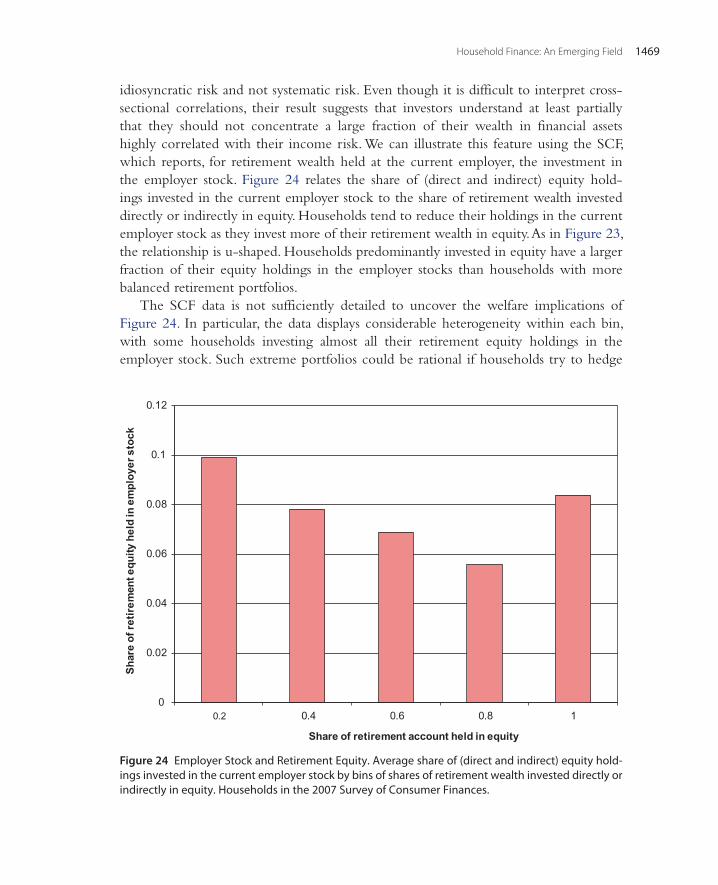
Household Finance: An Emerging Field 1469
idiosyncratic risk and not systematic risk. Even though it is difficult to interpret cross-sectional correlations, their result suggests that investors understand at least partially that they should not concentrate a large fraction of their wealth in financial assets highly correlated with their income risk. We can illustrate this feature using the SCF, which reports, for retirement wealth held at the current employer, the investment in the employer stock. Figure 24 relates the share of (direct and indirect) equity hold-ings invested in the current employer stock to the share of retirement wealth invested directly or indirectly in equity. Households tend to reduce their holdings in the current employer stock as they invest more of their retirement wealth in equity. As in Figure 23, the relationship is u-shaped. Households predominantly invested in equity have a larger fraction of their equity holdings in the employer stocks than households with more balanced retirement portfolios.
The SCF data is not sufficiently detailed to uncover the welfare implications of Figure 24. In particular, the data displays considerable heterogeneity within each bin, with some households investing almost all their retirement equity holdings in the employer stock. Such extreme portfolios could be rational if households try to hedge
0
0.02
0.04
0.06
0.08
0.1
0.12
0.2 0.4 0.6 0.8 1
Shar
e of
retir
emen
t equ
ity h
eld
in e
mpl
oyer
sto
ck
Share of retirement account held in equity
Figure 24 Employer Stock and Retirement Equity. Average share of (direct and indirect) equity hold-ings invested in the current employer stock by bins of shares of retirement wealth invested directly or indirectly in equity. Households in the 2007 Survey of Consumer Finances.

Luigi Guiso and Paolo Sodini1470
their relative wealth in the local community (DeMarzo, Kaniel, and Kremer, 2004) or if they hold superior information on their employer stock (Van Nieuwerburgh and Veldkamp, 2010). Additionally, top managers might be required to hold a large fraction of their wealth in the employer stock to align their incentives with shareholder interests (Frydman and Jenter, 2010). However, it could also be that households with most of their retirement wealth invested in the employer stock are the poor and uneducated, choosing financial assets as they choose any other consumer product—out of familiarity, loyalty, or simply because it makes them feel good.
4.2.3 Frequency and Profitability of TradingIn the standard Merton (1969) model, the vector of portfolio shares invested in risky assets by a household i with relative risk aversion γi is:
where Erei is the vector of expected risky asset excess returns and �i is the variance-
covariance matrix of the vector of excess returns. One of the features of this frictionless, partial equilibrium model, is that any news that results in a change of Ere
i or �i, induces household i to immediately reallocate its portfolio. This carries two implications. First, the frequency with which an investor obtains news and the frequency of trading should coincide. Second, events that affect household relative risk aversion γi, such as variations in wealth or background risk, should induce households to reduce proportionally the investment in all risky assets. The basic Merton model suggests, then, that households should rebalance and reallocate their portfolio very frequently, if not continuously. In this section, we review the evidence on the frequency and profitability of individual investor trading activity.
Table 7 is an excerpt from the appendix of Alvarez, Guiso, and Lippi (2012) and reports the average yearly number of trades for households in the UCS survey. On average, households trade 4.5 times per year, with direct stockholders trading 6 times. The distribution is skewed (the median is 3.4, and 5.8 for direct stockholders) and substantially dispersed (the standard deviation is 3.7, and 3.4, respectively). Most of the trades are either assets sales—that is trades involving a sale of some investment against cash—or assets purchases—trades involving a purchase of some financial assets with cash. On average, rebalancing trades are 20% of the total number of trades in the whole sample and 30% among direct stockholders. In contrast to the predictions of the fric-tionless model, Table 7 highlights that households do not trade frequently—less than once every couple of months on average—and only a minority of households churn their portfolios. Alvarez, Guiso and Lippi (2012) report also data on the frequency people check their investments. They show that investors also observe their portfolio infrequently, about 12 times in a year for the median investor, as would be predicted by
(4.2)ωi =1
γi�−1
i Erei ,

Household Finance: An Emerging Field 1471
models with costly information gathering or attention costs. Furthermore, frequency of trading and frequency of observations are strongly positively correlated, investors tend to observe their investments more frequently than they trade and only very rarely they trade without first checking on their investments.
To account for these facts, a growing literature augments the Merton model with trading and observation costs43 which, coupled with consumption of durables, can account for the trading and observation patterns observed in the data (Alvarez, Guiso and Lippi 2012).
If households were able to process news correctly, they would trade on information only when it is profitable and, as a consequence, earn higher returns per unit of risk than uninformed investors (Brunnermeier, 2001). We have seen in Section 4.2.2, that there is mixed evidence on whether households are able to profit by buying familiar stocks. What do we know about trading profitability in general? Do households trade efficiently on information, or do they suffer from behavioral biases, such as overconfi-dence, and trade too much as a consequence? In the reminder of this section we briefly review the literature.
On average, individual investors tend to suffer trading losses, even before fees and partic-ularly in the long run (Barber and Odean, 2000; Grinblatt and Keloharju, 2000). However, the average behavior conceals high heterogeneity in trading performance across investors. Those who trade more frequently tend to earn lower returns after fees (Barber et al., 2009), with men more prone to trading and to losses than women (Barber and Odean, 2001).
43 See, among others: Duffie and Sun (1990), Gabaix and Laibson (2001), Sims (2003), Reis (2006), and Abel, Eberly, and Panageas (2007, 2009).
Table 7 Trading Frequency. Summary statistics for the yearly number of trades, number of trades that are sales of assets and number of trades that are purchases of asset in the whole sample as well as in the sample of stockholders. The latter are defined based on whether the investor owns stocks directly (direct stockholders) and directly or indirectly (total stockholders) Source, Alvarez, Guiso, and Lippi (2012) Median Mean Std. Dev.
All trades (NTj) 3.40 4.50 3.70Of which asset Sales (NSj)
1.40 2.00 2.00
Of which asset Purchases (NPj)
2.40 3.60 3.60
Stockholders (NTj) 5.10 5.80 3.60(direct+indirect) Stockholders (NTj)(direct)
5.80 6.00 3.40
Luigi Guiso and Paolo Sodini1472
A minority of investors are instead able to earn positive risk-adjusted returns and persis-tently do so. Barber et al. (2011a) find that the top 500 Taiwanese day traders are able to reliably earn positive abnormal returns net of trading costs over time. Grinblatt, Keloharju and Linnainmaa (2012) find that investors with higher IQ are more likely to achieve posi-tive performance, they manage taxes more efficiently, sell at high prices, have superior mar-ket timing, stock picking skills, and trade execution. Finally, a few recent papers document that investors seem to learn from past experiences; they quit trading after experiencing consistent losses over time (Barber et al., 2011b; Nicolosi, Peng, and Zhu, 2009).
One pervasive common trading pattern among individual investors is the disposition effect, the tendency to realize losses too late and gains too early (Grinblatt and Keloharju, 2001b; Odean, 1998; Shefrin and Statman, 1985). There is a growing debate on the determinants of the disposition effect. Originally, it has been attributed to prospect theory preferences, but Barberis and Xiong (2012) have recently argued that this is not necessarily the case, especially if preferences are defined over annual gains and losses.44 There is growing evidence that more sophisticated investors are less prone to the dis-position effect (Dhar and Zhu, 2006, and Grinblatt, Keloharju, and Linnainmaa, 2012), a finding which is consistent with a behavioral explanation. Calvet, Campbell, and Sodini (2009a) point out that the disposition effect is consistent with portfolio rebalanc-ing and find that wealthier investors with better diversified portfolios tend to behave symmetrically when selling winning and losing stocks, and are thus less prone to the disposition effect. They also document no asymmetries in mutual fund sales depending on past performance, suggesting that the disposition effect is a phenomenon limited to direct stock holdings.
In summary, households trade infrequently on average but a minority of them churn their portfolios. There is large cross-sectional heterogeneity in trading performance with the average investors suffering trading losses even before fees. Investors who trade more suffer larger trading losses net of fees but they seem to learn from past experience and sub-sequently quit the market. Sophisticated investors earn reliable positive abnormal returns over time and are less prone to behavioral trading patterns, such as the disposition effect.
4.2.4 Delegation of Portfolio Management and Financial AdviceRather than deciding on their finances directly, households may delegate portfolio deci-sions to professional money market managers and, when deciding on their own, rely on the suggestions of financial advisors. Economies of scale in expertise, information col-lection and transaction costs make the market for financial expertise suitable to improve household finances and welfare. Indeed, about 60% of the investors in the 2007 UCS
44 Two prominent behavioral explanations of the disposition effect are that investors have an irrational belief in mean-reversion, or that they derive utility directly from realizing gains and losses, a notion labeled “realization utility” by Barberis and Xiong (2009).

Household Finance: An Emerging Field 1473
survey rely on the help of an advisor or intermediary when making financial decisions and only 12% decide on their own without counsel. Hung et al. (2008) report that 73% of US investors rely on professional advice to conduct stock market or mutual fund transactions. However, adverse selection among mutual fund managers (Berk and Green, 2004), conflict of interest with financial advisors (Inderst, 2010; Inderst and Ottaviani, 2009, in press,) and lack of financial literacy among households (Lusardi, Mitchell, and Curto, 2009, 2010) might generate suboptimal equilibria that may require regulatory intervention (Campbell, Giglio, and Pathak, 2011).
Portfolio Delegation. A large and long-standing literature studies the determinants of mutual fund performance and net flows. After fees, actively managed mutual funds do not achieve a higher performance than passive indexes on average, and their risk adjusted returns display little persistence over time (Carhart, 1997; Fama and French, 2010; Jensen, 1968; Wermers, 2000). Net flows seem to correlate with past returns par-ticularly for well-performing funds (Chevalier and Ellison, 1997; Huang, Wei, and Yan, 2007; Lynch and Musto, 2003; Sirri and Tufano, 1998).
Only a handful of papers, instead, have more recently been using data on individual investor behavior to study the micro-determinants of mutual fund flows. By using information on US individual brokerage accounts, Ivkovic and Weisbenner (2009) are able to study inflows and outflows separately, and find that inflows are driven by relative performance measures and outflows instead react to absolute levels of past returns. They also find that investors pay attention to taxes and fees in deciding how to trade fund shares. Past performance and shares redemptions are positively correlated for funds held in taxable accounts but uncorrelated in tax-deferred accounts, a finding in stark contrast to the disposition effect that individual investors display in their direct stockholdings (see Section 4.2.3). As we would expect, fees in percentage of assets under managements encourage redemptions, whereas front-loads induce investors to hold on their fund shares, even though upfront costs should be considered sunk costs. Choi, Laibson, and Madrian (CLM, 2010) conduct an experiment that builds on the finding that the cross-sectional variation in fees charged by S&P 500 index funds is surprisingly similar to the variation found in actively managed funds (Hortaçsu and Syverson, 2004).45 Subjects are asked to invest 10,000 USD hypothetically between four real S&P 500 funds with their experimental earnings depending on how well their chosen portfolio performs subse-quently. They find that only a minority of investors minimize fees and instead that most investors seems to pay attention predominantly to past returns. They attribute the sub-optimal behavior to mistakes since more literate investors are more likely to choose lower fees, and those who do not minimize fees are more likely to feel afterwards that they have not taken the best decision. In line with CLM, 2010, Grinblatt et al. (2011)
45 Kahraman (2009) finds that a substantial fraction of the documented fee dispersion in S&P 500 index funds arises within funds rather than across funds due to the variation in multiple class shares.

Luigi Guiso and Paolo Sodini1474
find that investors with higher IQ seem to minimize fees when choosing across mutual funds. Bailey, Kumar, and Ng (2011) relate the mutual fund choices of the clients of a large US brokerage house to the behavioral biases they display in individual stock trad-ing. They find that less sophisticated and behaviorally biased investors are more likely to choose mutual funds poorly across a number of dimensions such as fees, trading fre-quency, timing, and performance.
Financial Advice. The early literature on financial advice (Barber et al. 2001a; Elton, Gruber, and Grossman, 1986; Womack, 1996) has primarily focused on the information content of analyst recommendations,46 and argued that security analysts seem to be able to predict stock returns, but their recommendations are difficult to be exploited after trading costs. More recently, a number of papers have studied other aspects of the financial advisory activity. In line with the analyst literature, Hackethal, Haliassos, and Jappelli (HHJ, 2011), and Kramer (2012) find that advised accounts do not earn higher raw and abnormal returns than non-advised accounts after fees and after controlling for investor characteristics. Even though advisors do not seem to improve client port-folio performance, they may still help investors to avoid common investment mistakes and mitigate behavioral biases. Shapira and Venezia (2001) and HHJ (2011) find that advised accounts have better diversified portfolios and are less prone to the disposition effect. Mullainathan, Nöth, and Schoar (MNS, 2009) find the opposite result by track-ing the recommendations that trained auditors, acting as customers, receive from finan-cial advisors. The auditors are assigned different portfolios characterized by various biases and are sent to seek advice from advisors with contrasting or aligned incentives. Even though it is not clear whether in a long-term client relationship the audited advi-sors would keep the same suggestions, MNS (2009) find that existing biases are, if anything, augmented by professional advisors. Bluethgen, Hackethal, and Meyer (2008) indeed find large heterogeneity in the quality of financial advisors not only due to skill but also to the form of compensation. Advisors that receive fixed fees rather than sale commissions tend to offer better recommendations. Consistently, HHJ (2011) find that account performance is higher when managed by independent, rather than bank, financial advisors.
Some of the findings reported above are difficult to interpret solely as the outcome of financial advisor skills and incentives. Indeed the group of individuals that seek and end up using financial recommendations might not be representative of the popula-tion and might not be randomly matched to financial advisors. A robust finding is that more sophisticated (wealthier, better educated, more financially literate, less overcon-fident) and more trusting investors are more likely to delegate portfolio management
46 See Mehran and Stulz (2007) for a review of the literature within the broader context of conflict of interest in financial institutions.

Household Finance: An Emerging Field 1475
or seek financial advice (Bucher-Koenen and Koenen, 2010; Georgarakos and Inderst, 2011; Guiso and Jappelli, 2006; HHJ (2011)). Bhattacharya et al. (2011) perform a randomized experiment whereby unbiased financial advice is offered to a sample of randomly selected customers of a large European brokerage house. Despite the fact that the advice is unbiased by construction and is given for free, the offer is accepted only by 5% of the 8,000 contacted clients. In line with the previous literature, financial sophistication increases the probability of accepting the advice but, surprisingly, makes it also less likely that the advice is followed. Taken literally, these results suggest that improving financial advice quality might not have a large impact on investor welfare, those who accept the advice are those who need it the least and who are less likely to follow the advice ex post.
4.3 Portfolio Rebalancing in Response to Market MovementsIn Section 3, we have studied financial risk taking in a static framework. In this and the next sections we turn to portfolio allocation dynamics and study rebalancing and participation turnover. First we investigate how households change their financial risk exposure in response to market movements, then, in the next section, we study rebal-ancing and participation decisions over the life-cycle.
The popular practitioner recommendation of rebalancing the portfolio so that the share invested in risky assets is stable over time is most likely rooted in the theoretical predictions of the basic partial equilibrium Merton model. As we saw in (3.1), household i should choose a risky share ωi equal to a target risky share ω∗
i = Erei /(γiσ
2i ) that depends on its relative risk aversion γi and its beliefs about the
market risk-return trade-off Erei /σ
2i . Movements in asset prices mechanically induce
passive variations of the risky share ωi that might not coincide with revisions of the target share ω∗
i . The practitioner advice is then based on the assumption that investor beliefs and risk aversion remain unchanged. In this case, the risky share ωi should be rebalanced back to its original level and should fully offset the variations induced by asset price movements.
Such a conclusion, however, not only assumes that households do not revise their target shares over time, but also does not take into account the reaction of asset prices to household rebalancing. In equilibrium, no aggregate rebalancing is possible. The average household has to hold the market portfolio and its risky share can only change passively with asset prices. Yet, in a heterogeneous agent economy, the aggregate inertia conceals the trading activity of investors with different information (and beliefs) or different risk aversion. Uninformed investors absorb the trades of the informed, and thus rebalance by engaging in contrarian trading, i.e. by buying when prices fall and selling when prices rise (Grossman, 1976; Grossman and Stiglitz, 1976). Kimball, Shapiro, and Zhang (2011) show that in an exchange economy with symmetric information, more risk averse investors are also forced to follow contrarian rebalancing in equilibrium.

Luigi Guiso and Paolo Sodini1476
Do households rebalance their portfolios actively or do they let their portfolio alloca-tions vary passively with market prices? Which households rebalance more actively? Do they follow contrarian or momentum strategies? Do they rebalance stock and mutual fund holdings in the same way, or do they trade in the two types of securities differ-ently? In the remainder of the section we review the empirical evidence on households rebalancing in response to changes in asset prices.
Rebalancing individual positions. One strand of the literature uses data that identifies trades on single stocks by individual investors at stock exchanges. High frequency net trades of individual investors are aggregated at stock level and are correlated to the stock past performance. A widespread finding across countries and exchanges is that individual investors as a group tend to be contrarian investors at least over the horizon of up to one year (see, among others, Choe, Kho, and Stulz, 1999; Griffin, Harris, and Topaloglu, 2003; Goetzmann and Massa, 2002 and Richards, 2005).
This finding is confirmed on data with information at individual investor and stock level. Grinblatt and Keloharju (2000, 2001b) document that Finnish investors follow contrarian strategies with respect to short and intermediate horizon (up to one year). The contrarian trading behavior is stronger for small stock investments and varies across investors. Households, government institutions, and non-profit organizations are more prone to contrarian strategies than finance companies, insurance institutions, and for-eigners. A fact that can be interpreted as evidence that more sophisticated investors are less likely to be contrarian investors. Calvet, Campbell, and Sodini (CCS, 2009a) find evidence that Swedish households rebalance by offsetting about one sixth of the passive variations in the share of risky assets invested in a single stock.
Rebalancing the financial portfolio. All these findings pertain to trading in individual stocks. They do not tell us how these trades relate to rebalancing of the overall risky share ωi and how rebalancing itself correlates with household characteristics. CCS (2009a) attempt to fill this gap using data from the Swedish Wealth Registry. By using information on household portfolio holdings at individual asset level at the end of each year, they decompose the observed yearly changes of the risky share �ωi into passive and active variations:
The passive variation �ωpi is the change in the risky share that would have occurred if
households were fully passive and did not buy or sell securities during the year. Hence �ωpi
is the change in the risky share purely and solely induced by changes in asset prices. The active variation �ωa
i is the residual change, and is instead fully driven by household decisions.Consistent with markets being in equilibrium, CCS (2009a) find that active variations
in the aggregate risky share of Swedish households are small but at the same time hide strong rebalancing at individual investor level. Households hold diverse portfolios and therefore experience different passive variations in their risky share. As a result, households
�ωt = �ωpi + �ωa
i .

Household Finance: An Emerging Field 1477
have different incentives to rebalance their portfolio and thus trade with each other. CCS (2009a) exploit this heterogeneity by regressing active on passive variations of the risky share and estimate a rebalancing coefficient of approximately minus one-half.47 Households offset about 50% of the passive variations in their risky asset share and thus follow a strong contrarian strategy not only when trading individual stocks, as shown in the previous literature, but also in their overall portfolio risk taking behavior.
In order to identify how households rebalance their portfolios, CCS (2009a) classify households into lucky and unlucky, depending on whether the return on their risky assets is above or below the population average. They decompose the rebalancing coef-ficient of minus one-half into the contribution of lucky and unlucky households and, in turn, into eight trading strategies. They distinguish between trades in stocks and in funds, between full and partial sales, and full and partial purchases. As implied by equi-librium conditions, lucky and unlucky households have similar rebalancing coefficients but they use different trading strategies. Lucky households, which need to reduce their holdings of risky assets, rebalance by fully selling stocks and by buying less into mutual funds. Unlucky households, instead, increase their asset holdings by buying more risky assets, primarily stocks, both fully and partially.
As we already pointed out at the beginning of this section, the popular recommen-dation of rebalancing towards a stable risky share assumes that households do not change risk attitudes and beliefs over time. Limited rebalancing may well be optimal for house-holds who revise their target share ω∗
i substantially. It is then unclear whether the esti-mated rebalancing propensity of minus one-half is the result of households trading towards a revised target share ω∗
i or of inertia in portfolio rebalancing. To shed light on this issue, CCS (2009a) propose a simple adjustment model of portfolio rebalancing in which investors have different speed of adjustments φi towards their optimal target share ω∗
i . Investors with unit speed of adjustment, φi = 1 rebalance instantaneously and their observed share ωi is equal to target share ω∗
i at all times. Investors with zero speed of adjustment, φi = 0, do not rebalance their portfolio at all, and their observed risky share ωi is always equal to their passive share ωp
i .48 CCS (2009a) estimate a structural model
and find that, (a) the average speed of adjustment is about three-quarters, and (b) inves-tors revised their target share downwards by about 15% during the bear market of 2001 and 2002 in Sweden. They also find that richer, more educated households with better diversified portfolios have a higher speed of adjustment, and that households that became richer revised their targets upwards. Their results indicate that more sophisticated house-holds rebalance more efficiently and confirm the findings of Section 3.2.1 in support
47 They control for the risky share at the beginning of the year and find the same result for a log specifica-tion of the regression. They also find that the estimated coefficient of −1/2 is robust to the inclusion of household characteristics in the regression.
48 In the Swedish Wealth Registry, ωpi can be calculated from the household observed initial risky share ωi,0
and the risky share passive variation �ωpi as ω
pi = ωi,0 + �ω
pi .

Luigi Guiso and Paolo Sodini1478
of DRRA preferences. Figure 25, taken from table A11 of the online appendix to CCS, (2009a), illustrates the relationship between sophistication and rebalancing. The figure classifies households into adjustment speed bins, and reports the fraction of households with high-school and post high-school education in each bin. The relation between education and rebalancing is strong. The fraction of households with post high-school education is only 6% in the 5th percentile of the speed of adjustment distribution, and climbs to 71% in the 95th percentile.49
In the presence of trading and participation costs, the Merton model implies that some households enter and exit risky asset markets over time. Hurst, Luoh and Stafford (1998) and Vissing-Jørgensen (2002) have documented that, in the US, the popula-tion of participants is not stable but characterized by substantial turnover. The same demographic characteristics that predict participation, such as income, wealth, and education, also predict a higher probability of entry and a lower probability of exit. CCS, (2009a) additionally relate exit decisions with investor portfolio characteristics. They find that households with higher risk exposure and better diversified portfolios are less likely to exit. They also document that the decision to exit is not uniform across types of assets. Households are more likely to stop holding single stocks if they have performed well but they are more likely to sell all their funds after they have performed badly.
Even though understanding how households react to changes in market conditions is a central issue in financial economics, asset pricing models have so far mostly concen-trated on different issues than rebalancing behavior, and the empirical literature is still identifying the basic stylized facts. An established finding is that households follow con-trarian strategies on average both at individual stock level and when they rebalance the share of financial wealth invested in risky assets. The most recent evidence suggests that households offset about 50% of the idiosyncratic passive variations in their risky share, with more sophisticated investors rebalancing faster. Additionally households rebalance by using a variety of trading strategies that are not symmetric across stocks and funds, and differ depending on past portfolio performance.
4.4 Portfolio Rebalancing Over the Life-CycleIn the past ten years a number of contributions have re-examined the life-cycle behav-ior of investor portfolios. Inspired by empirical findings from novel microeconomic data on household finances, several papers have provided new models of optimal portfolio
49 Inertia in portfolio rebalancing does not only vary with household characteristics but seems to vary across types of savings. The findings of CCS (2009a) apply to household current financial wealth invested in stocks and funds and lie in between two other findings in the literature. Individual investors are very active when trading in stocks through brokerage houses (e.g. Odean, 1999) and instead display strong inertia in their 401k pension accounts (e.g. Carroll et al. 2009; Choi et al. 2009).
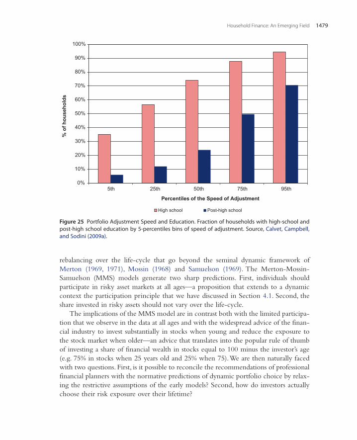
Household Finance: An Emerging Field 1479
rebalancing over the life-cycle that go beyond the seminal dynamic framework of Merton (1969, 1971), Mossin (1968) and Samuelson (1969). The Merton-Mossin-Samuelson (MMS) models generate two sharp predictions. First, individuals should participate in risky asset markets at all ages—a proposition that extends to a dynamic context the participation principle that we have discussed in Section 4.1. Second, the share invested in risky assets should not vary over the life-cycle.
The implications of the MMS model are in contrast both with the limited participa-tion that we observe in the data at all ages and with the widespread advice of the finan-cial industry to invest substantially in stocks when young and reduce the exposure to the stock market when older—an advice that translates into the popular rule of thumb of investing a share of financial wealth in stocks equal to 100 minus the investor’s age (e.g. 75% in stocks when 25 years old and 25% when 75). We are then naturally faced with two questions. First, is it possible to reconcile the recommendations of professional financial planners with the normative predictions of dynamic portfolio choice by relax-ing the restrictive assumptions of the early models? Second, how do investors actually choose their risk exposure over their lifetime?
0%
10%
20%
30%
40%
50%
60%
70%
80%
90%
100%
5th 25th 50th 75th 95th
% o
f hou
seho
lds
Percentiles of the Speed of Adjustment
High school Post-high school
Figure 25 Portfolio Adjustment Speed and Education. Fraction of households with high-school and post-high school education by 5-percentiles bins of speed of adjustment. Source, Calvet, Campbell, and Sodini (2009a).

Luigi Guiso and Paolo Sodini1480
4.4.1 Earlier Frictionless ModelsThe earlier contributions should be viewed as establishing the benchmark conditions under which a long-term investor would choose “myopically”. As Samuelson (1969) points out, “[A] lifetime model reveals that investing for many periods does not in itself introduce extra tolerance for riskiness at early, or any stages of life.” Under the MMS assumptions of no labor income, unpredictable stock returns, constant relative risk aversion, and time-separable preferences, there is no horizon effect in that the optimal portfolio risky share does not vary with age. Jagannathan and Kocherlakota (1996), for example, dismiss the popular argument made by Malkiel (1996) in his famous book “A Random Walk Down Wall Street”, and adopted by many financial advisors, that most of the stock market risk can be eliminated if an investor has sufficiently many years ahead, since, if investors can rebalance their portfolio at no cost, the relevant horizon is between portfolio adjustments and not stages of the life-cycle. The MMS model provides a clean benchmark showing that this popular professional advice needs to be qualified in order to be justified. It lays down the foundations for asking which assumptions need to be relaxed in order to rationalize financial advisor recommendations.
Probably the most unrealistic assumption of the MMS benchmark is the absence of human capital. Labor income is by far the most important source of household income, and human capital represents a large fraction of total lifetime wealth for the vast major-ity of households (see Figure 2). Most importantly, human capital evolves over the life-cycle and is likely to affect optimal portfolio choice as individuals get older.
Consider the case of riskless constant labor income flow y over the investor lifetime. For an investor of age a and horizon T, human capital HC(a, T ), is given by:
i.e. it is the present value of future labor income discounted at the risk free rate rf . With constant deterministic labor income, human capital is at its maximum early in life, when there are many years of earnings ahead, and declines afterwards with age. Assuming trad-able labor income and complete markets, Merton (1971) shows that, for an investor i of age a with constant relative risk aversion γi and financial wealth Wi,a, the risky share is
where Erei is the expected risk premium and σi is the return volatility of risky assets. In
the absence of labor income, human capital is zero and the formula reduces to (3.1), the myopic solution we have so far considered. With labor income, the optimal risky share is increasing in the ratio of human wealth to financial wealth HC(a, T )/Wi,a and thus
HC(a, T ) =y(
1 − e−rf (T−a))
rf,
(4.1)ωi,a =Ere
i
γiσ2i
[
1 +HC(a, T )
Wi,a
]
,

Household Finance: An Emerging Field 1481
varies as this ratio evolves over the life-cycle. Early in life, when accumulated financial assets Wi,a are low and human capital HC(a, T ) is high, the ratio is high and households hold a large share of financial assets in risky securities. As households become older, they accumulate financial assets, their human capital declines and, as a consequence, they rebalance downwards their portfolio risky share. The intuition is simple. Since human capital is riskless and tradable, it has the same role of a large endowment in riskless bonds, and thus creates a strong incentive to invest in risky securities.50 As we shall see below, this basic intuition is very robust and it is one of the main features of calibrated optimal portfolio choice models over the life-cycle. The popular financial planners’ advice of investing heavily in risky assets early in life can then be rationalized by intro-ducing human capital in the basic Merton model.
4.4.2 Non-Tradable and Non-Insurable Labor IncomeThe assumption that human capital is tradable and insurable yields closed form solu-tions and thus facilitates the identification of the role of human capital in affecting portfolio rebalancing over the life-cycle. Yet, it is a strong assumption. Households tend to face, perhaps even more than firms, limited access to credit markets, particularly at the early stage of their life when they have few accumulated assets to offer as collateral. Insurability of labor income is equally problematic in light of the moral hazard prob-lems that wage and employment insurance entails. A new recent wave of papers has reconsidered the Merton (1971) model relaxing the assumption of complete markets and tradability of human capital.51 Most of these models do not have closed form solu-tions and have to be solved numerically.52 A representative example of this literature is Cocco, Gomes, and Maenhout (2005). They build and numerically simulate a life-cycle model of consumption and portfolio choice which allows for non-tradable and uncer-tain labor income as well as many other features that characterize a typical household environment such as bequest motives, mortality risk, non-standard preferences, uncer-tain retirement income and catastrophic labor income shocks. They calibrate the labor
50 Equation (4.1) is nothing more than (3.1) with the risky share defined as the proportion of total wealth (human and financial) invested in risky financial assets. Indeed, we can rewrite (4.1) as
ωi,aWi,a
HC(a,T )+Wi,a=
Erei
γiσ2i.
When HC(a, T ) is a large fraction of total wealth, the risky share ωi,a has to be very high, compared to the case without human capital, for the right-hand side to be equal to the target share Ere
i /(γiσ2i ).
51 See Heaton and Lucas (1997), Gakidis (1998), Haliassos and Michaelides (2001), Campbell and Viceira (2001), Viceira (2001), Gomes and Michaelides (2004 and 2005), Cocco, Gomes, and Maenhout (2005), Davis, Kubler, and Willen (2006), Benzoni, Collin-Dufresne, and Golstein (2007), Gomes, Kotlikoff, and Viceira (2008).
52 In this section, we discuss models that focus on optimal portfolio over the life-cycle in partial equilib-rium. Several papers have considered the asset pricing implications of life-cycle portfolio models with labor income and frictions. Among others, Heaton and Lucas (1977), Constantinides, Donaldson, and Mehra (2002), Storesletten, Telmer, and Yaron (2007).

Luigi Guiso and Paolo Sodini1482
income process on the US PSID and estimate average consumption and assets alloca-tion by simulating the model over 10,000 households. A robust prediction is that the portfolio share invested in stocks has a strong life-cycle profile. We reproduce the results for their benchmark case in Figure 26 which reports the life-cycle pattern of the port-folio share invested in stocks.
For the average household (continuous line), the risky share is very high and increas-ing at the very beginning of the life-cycle; very soon it hits the maximum level of 1 because of borrowing constraints. Around age 40, as the value of human capital starts decreasing and financial wealth grows, the household starts rebalancing its portfolio towards riskless bonds. At age 65, the portfolio share invested in risky assets reaches about 50%—half of the value when young. After retirement, the risk asset share is relatively stable (and even slightly increasing) since households start dissaving and both human capital and financial wealth decline. The rebalancing strategy over the life-cycle described above is fairly robust to a number of features such as bequest motive (Merton, 1971), pension income risk (CGM, (2005), Epstein and Zin (1989)) recursive utility (CGM, (2005); Gomes and Michaelides, 2005; Haliassos and Michaelides, 2001) and endogenous labor supply (Bodie, Merton, and Samuelson, 1992; Chan and Viceira, 2000; Gomes, Kotlikoff, and Viceira, 2008).
0
0.2
0.4
0.6
0.8
1
20 25 30 35 40 45 50 55 60 65 70 75 80 85 90 95
Ris
ky S
hare
Age
Figure 26 Life cycle profiles of portfolio risky share. The figure reproduces the simulations of the life cycle of the portfolio risky share of Cocco, Gomes, and Maenhout (2005)—baseline Figure 3 panel c.

Household Finance: An Emerging Field 1483
4.4.3 Addressing Counterfactual PredictionsEven though the models described in the previous section account for many realistic features of the household optimal portfolio life-cycle problem, they generate a number of counterfactual implications.
Too Large Share in Stocks when YoungAll the models of Sections 4.4.1 and 4.4.2 tend to predict very large portfolio risky shares or even short-selling for young households. This prediction is counterfactual: although it is true that the young tend to be more highly leveraged, very few of them have portfolio shares that even get close to those recommended by these models. For instance, in the last wave of the SCF only 12% of participating young households (those between 20 and 30) have a share in risky assets that exceeds 80%.
One avenue that has been pursued to address this issue is to allow for “disasters”, i.e. the possibility of a very large drop in labor income. For instance, CGM (2005) show that allowing for a small probability (0.5%) of a drop to zero in labor income lowers dramatically the share invested in equity at young age to a more reasonable level of 40%.53 The presence of extreme income losses creates a large background risk which reduces the optimal share in stocks. This effect is particularly important at young age, when the ratio of human capital to financial assets is large. It fades only later in life, when accumulated assets are larger compared to human capital, and thus fails to predict the observed lower risky shares of middle-age households.
A second mechanism that could potentially predict a lower risky share relies on the relation between the return of risky assets and human capital. A positive correlation between labor income and stock returns weakens the “bond-type” nature of human capital and turns it into an “equity-type” of asset, thus discouraging financial risk tak-ing. For some categories of investors, labor income can be highly correlated with stock returns—e.g. top managers whose compensation is tied to the value of the company, or employees who hold a large fraction of financial wealth in the employer stock (see Section 4.2.2). However, for many households income shocks arise mostly from health issues, local job market conditions, entrepreneurial risk and family composition dynamics. Innovations in earnings are thus idiosyncratic in nature (Heathcote, Storesletten, and Violantec, 2008) and should then be mostly uncorrelated with equity markets. Various studies document a low contemporaneous correlation between earn-ings and stock market returns. Davis and Willen (2000) find that innovations to labor income of ten US different occupations are not significantly correlated with contem-poraneous aggregate stock market returns, a result that Botazzi, Pesenti, and Wincoop
53 Allowing for disasters also raises portfolio heterogeneity at young age that in a standard model is (again counterfactually) very low.
Luigi Guiso and Paolo Sodini1484
(1996) confirm in several other countries. Lack of correlation between labor income and stock market returns is somewhat puzzling within the framework of general equi-librium asset pricing models with growth. Benzoni, Collin-Dufresne, and Golstein (2007) point out that focusing on the contemporaneous correlation between labor income and stock market returns, as many general equilibrium calibrated models do, and forcing it to be low imposes also a low long-term correlation.54 They instead argue that the relationship between labor income and stock market returns can be better represented by cointegration measures. Cointegration is consistent with the low contemporaneous correlations found in the data, but also with a significantly higher long-run correlation, as implied by the theoretical models. BCG (2007) find that the long-term correlation between labor income and stock returns generates a hump-shaped pattern of the portfolio share invested in equity over the life-cycle. When young, the horizon is long and the role of cointegration is important, so human capital behaves as equity and investors take less financial risk. As the horizon shortens, coin-tegration loses importance and the bond type role of human capital takes over, induc-ing households to hold more stocks. Though this mechanism can significantly lower the optimal share in stocks at young age, it still implies abnormally high shares at intermediate ages.
Finally, even without direct correlation between labor income and stock returns, countercyclicality in the volatility of idiosyncratic income risk can deter equity invest-ment (Constantinides and Duffie, 1996; Storesletten, Telmer, and Yaron, 2007). One way to think about this is that an increase in idiosyncratic income volatility increases the discount rate that an undiversified household applies to its labor income, and thereby lowers the value of human capital, lowering equity investment. If this occurs at the same time as the stock market declines, then human capital and the stock market are cor-related, but not because labor income itself is correlated with the market. Meghir and Pistaferri (2004) find empirical support for the countercyclical volatility of idiosyncratic income risk.
A third approach emphasizes borrowing costs. In a frictionless model, young investors would borrow at the risk free rate and invest in stocks in order to balance the high endowment of human capital. If borrowing costs are higher, the incentive to invest in risky assets weakens, and it disappears when the lending rate exceeds the equity premium. Davis, Kubler, and Willen (2006) argue that this mechanism mitigates stockholding at young ages.
54 The low correlation estimated in these studies may reflect the fact that no distinction is made between permanent and transitory shocks to labor income. Campbell et al. (2001) distinguish between correlation of stock returns with permanent and transitory income shocks. They find a positive and large correlation of stock returns with the permanent aggregate component of labor income shocks.

Household Finance: An Emerging Field 1485
Absence of Limited ParticipationThe Merton (1971) model of (4.1) implies that all households invest in risky securities. This prediction is at odds with lack of participation at all ages and in particular with the low participation rates of young households (see Figure 28a below). The introduc-tion of a one-time fixed participation cost (e.g. Gomes and Michaelides, 2005) helps in explaining the limited participation of the young, since early in life households have not yet accumulated substantial financial wealth. However, fixed costs cannot deter partici-pation of the middle aged for reasonable calibrations of relative risk aversion parameters. GM (2005) argue that adding some heterogeneity in risk aversion can match the par-ticipation rates observed in the data. Households with lower risk aversion accumulate less precautionary assets (because risk aversion and prudence co-vary) and thus are less likely to enter. The opposite is true for those with high risk aversion. A heterogeneous economy with enough agents of the first type reproduces the participation structure in the data but also generates a negative correlation between risk tolerance and stock market participation, which is not supported empirically (e.g. Guiso and Paiella, 2008; Haliassos and Bertaut, 1995).
Interestingly, the two mechanisms cited in the previous section—costly borrowing and cointegration of earnings and stock returns—may induce limited participation even with-out fixed participation costs (Benzoni, Collin-Dufresne, and Golstein, 2007; Davis and Willen, 2000). Their effect can induce young households to short-sell stocks and, with short-selling constraints, to stay out of risky asset markets. However, costly borrowing and cointegration cannot explain the lack of participation at all ages, and, most importantly, that some households exit equity markets as they become older (Guiso, Jappelli and Pistaferri, 2002, and Figure 28a below). We will return to these issues below, in Section 4.4.5.55
4.4.4 Welfare ImplicationsThe normative models of portfolio rebalancing reviewed above can be also used to evalu-ate the welfare losses that households may incur if they depart from the optimal recom-mended portfolio allocation rule, for instance, because ill advised or because enrolled in a default investment plan. Gomes, Kotlikoff, and Viceira (2008) investigate the welfare costs of departing from the optimal solution of the CGM (2005) model augmented with flex-ible labor supply. They find that life-cycle funds designed to match investor risk tolerance
55 The presence of housing is another channel that can temper incentives to invest in stocks when young and strengthen incentive to stay out of the stock market. Cocco (2005) and Yao and Zhang (2005) embed residential real estate in a life-cycle model of consumption and portfolio choice with labor income. They find that, because of housing, young households have limited wealth to invest in stocks and thus are less likely to participate. Additionally, given the illiquid nature of housing wealth, house price risk crowds out stockholdings and reduces financial risk taking when real estate wealth is large compared to financial wealth and human capital. Thus, accounting for housing wealth contributes to correct both excessive participation and larger shares in stocks that the CGM (2005) type of models generates.

Luigi Guiso and Paolo Sodini1486
and investment horizon have small welfare costs. However, all other policies, including life-cycle funds which do not match investors’ risk tolerance, can have substantial welfare costs. For instance, a time-invariant 100% bond allocation can result in a welfare loss as large as 46% of income at the beginning of the life-cycle if the investor relative risk aversion is 5—and no less than 22% for investors with lower or higher risk aversion of 2 and 8 respectively. A constant 50–50 allocation rule, between bonds and stocks, results in a welfare loss of 15% of income for investors with risk aversion of 2, and 87% for inves-tors with a high risk aversion of 8. These calculations suggest that default rules can cause significant welfare losses if applied to an heterogeneous pools of investors, and that these losses should be weighed against the benefits that the default rule is meant to generate.
4.4.5 Other FactorsThe models, discussed so far, all rely on life-cycle patterns of labor income to induce portfolio rebalancing over the lifetime. There are however other factors that can contribute to time-varying optimal portfolio policies.
Non-CRRA PreferencesNon-CRRA preferences may generate rebalancing over the life-cycle. For instance, if individuals have hyperbolic Bernoulli utility
Merton (1971) shows that the optimal portfolio risky share depends on age even with-out labor income:
With η > 0, older investors take less financial risk than the young. Gollier and Zeckhauser (2002) consider a general characterization of risk tolerance and show that departure from linearity generates age effects. They show that younger agents have stronger incentives to take on risk if absolute risk tolerance is convex, whereas the opposite is true if absolute risk tolerance is concave (see Section 3.2.1 for evidence on the functional form of risk aversion).
Life-Cycle Patterns in Risk Aversion and Background RiskIndividual risk preferences are likely to change over the lifetime. Indeed, empirical studies find that elicited risk aversion parameters tend to increase with age (see Section 3.2.2), even though the estimated variation does not seem to be sufficient to
u(ci) =γi
1 − γi
(
βci
γi+ η
)1−γi
(4.2)ωi,a =Ere
i
γiσ2i
[
1 +ηγi
β
(1 − e−r f (T−a)
rf Wi,a
]

Household Finance: An Emerging Field 1487
explain the decline in the portfolio risky shares recommended by financial advisors, or implied by calibrated normative models such as CGM, (2005) and Gomes and Michaelides (2005).
The variation in background risk over the life-cycle might be an additional chan-nel through which risk taking behavior depends on age. Family composition might carry higher uncertainty early in life, for instance because the probability of divorce is higher and household size is still uncertain. Human capital is also likely to be riskier earlier in life. At the beginning of the working life, individuals face a wide range of possible career paths and therefore higher uncertainty. Later on, by choice or chance, some of the original opportunities are no longer available and individuals eventually settle in jobs with better defined income profiles. Additionally, unemployment risk is arguably higher at young age. Employers may prefer to lay off workers with short tenure, because of asymmetric information or job market regulations prescribing last-in-first-out rules. Guiso, Jappelli, and Pistaferri (2002) construct measures of back-ground risk from elicited subjective probability distributions of future earnings in a sample of Italian workers. Figure 27 reproduces the age profiles of elicited unemploy-ment probability and earning uncertainty computed using kernel regressions on age and education.56
Perceived income risk varies considerably over the life-cycle. The probability of unemployment declines for both education groups, but faster for individuals with higher education. Earning uncertainty follows a similar pattern, even though the decline is less marked. The findings highlighted in Figure 27 might have large quantitative effects in view of the CGM (2005) result that a small probability of extreme income losses has a strong impact on portfolio choice.
Polkovnichenko (2007) explores another channel that can potentially affect the effect of human capital on risk taking at young ages. He extends the model of CGM (2005) to endogenous habit formation preferences. The evolution of the habit to wealth ratio affects risk aversion over the life-cycle following the mechanism that we have highlighted in Section 3.3 (see (3.4)). When the habit is high compared to avail-able resources, investors are more risk averse for fear of not being able to sustain the same habit level in the future. This mechanism is particularly powerful in reversing the “bond type” effect of human capital on portfolio risk taking for young house-holds, since they both have high human capital and a high habit to wealth ratio. In his calibration exercise, Polkovnichenko (2007) indeed finds that young households take more conservative investment strategies than in a model with CRRA prefer-ences, since they have not yet accumulated enough wealth to sustain consumption sufficiently above habit.
56 Since the profiles are obtained from cross-sectional data, one should be cautious in interpreting them as reflecting only age effects, as they could also capture cohort effects.

Luigi Guiso and Paolo Sodini1488
Probability of unemployment
Earnings uncertainty
0
0.1
0.2
0.3
0.4
0.5
20 25 30 35 40 45 50
Prob
abili
ty o
f une
mpl
oym
ent
AgeUnemployment propability: high education
Unemployment propability: low education
0.02
0.03
0.04
0.05
0.06
20 25 30 35 40 45 50
Earn
ings
unc
erta
inty
AgeEarning Uncertainity: high education Earning Uncertainity: low education
(a)
(b)
Figure 27 Earnings uncertainty for low and high education over the life cycle. The first panel shows the subjective probability that a person of a given age loses his job over a 12 month horizon for high education (high school and college degree) and low education workers (less than high school). The second panel reports the age profile of earnings uncertainty for the same two groups of workers. Wage uncertainty is the coefficient of variation of the workers subjective earnings distribution one year ahead. See Guiso, Jappelli, and Pistaferri (2002) for details.

Household Finance: An Emerging Field 1489
Predictability of Stock ReturnsOne of the assumptions that produce the myopic solution of (3.1) is the lack of stock return predictability. Papers that relax this assumption (see for instance, Campbell and Viceira, 1999, 2002, and Kandel and Stambaugh, 1996) show that predictability in stock returns induces horizon effects. In particular, if stock returns are negatively serially cor-related, it is optimal to reduce the portfolio risky share as the investment horizon shortens.57
4.4.6 What Does the Empirical Evidence Tell Us About the Portfolio Life-Cycle?Micro-data on household portfolios tend to show two remarkable features. First, par-ticipation in the stock market is limited at all ages and tends to follow a life-cycle pattern—in many instances a hump-shaped one as documented for several countries by Guiso, Jappelli, and Pistaferri (2002). Second, the portfolio share invested in stocks tends to vary with age, though in this case the specific empirical pattern is more con-troversial. Summarizing the evidence for several countries, Guiso, Jappelli, and Pistaferri (2002) argue that the age profile of the risky share conditional on participa-tion is relatively flat, though in some instances “ … there does seem to be some mod-erate rebalancing of the portfolio away from risky securities” as investors age. The evidence on the risky share is clearly at odds with the implications of the life-cycle models with labor income discussed above, since these models uniformly predict a declining profile of the risky share as human capital becomes a smaller component of household total wealth. And since the cause of the decline in the share—the shrinking pattern of human wealth over the life-cycle—is an undisputed fact, one may wonder about the reliability of the finding that the risky share does not vary over the life-cycle. In addition, the empirical results are also at odds with the direct relation between human capital and financial risk taking found by Calvet and Sodini (in press). They use administrative data on the portfolios of Swedish twins and estimate a positive causal effect of a measure of human wealth, similar to the one used in Figure 1, on both participation and the risky share.58
There are at least three reasons to doubt the empirical findings on participation and risk taking over the life-cycle. First, most of the available evidence is obtained from cross-sectional data. Since in a cross-section one has to compare portfolio holdings of individuals of different ages at each point in time, one cannot separate age effects from cohort effects. Any pattern observed in participation or portfolio risky share may not reflect a life-cycle effect but differences across cohorts. Second, most studies ignore the fact that the risky portfolio share is only defined for participants and that
57 Notice that parameter uncertainty and learning effects offset mean-reversion in stock returns, although the magnitude of this is disputed (Barberis, 2000; Wachter and Warusawitharana, 2009).
58 See Section 3.2.1 for a discussion of twin regressions.

Luigi Guiso and Paolo Sodini1490
participation in assets markets is an endogenous choice. Third, the evidence comes primarily from surveys which are notoriously subject to potentially large measurement errors. Most importantly, measurement errors are likely to be more severe for older individuals since they are known to be correlated with wealth levels.
One notable exception to the cross-sectional approach is Ameriks and Zeldes (2004). They use a panel of TIAA-CREF contributors from 1987 to 1999. Since they can observe each individual in their sample for many periods, they can improve on the cross-sectional approach and shed some light on the age, time, and cohort effects. Additionally, the administrative nature of the data is likely to reduce measurement errors to a minimum. Of course, given that time, age, and year of birth are linearly related, they cannot be separated without restricting them in some way. Using a variety of identifying assumptions to separate age, time, and cohort effects, and distinguishing between stock ownership and conditional portfolio shares, they conclude that the life-cycle pattern of stock market participation is hump shaped, and the conditional share invested in stocks shows little variation over the investor lifetime.
While the study by Ameriks and Zeldes (2004) represents a clear step forward, there are a number of open issues which may affect their findings. First, TIAA-CREF only reports assets contributed to the retirement program, not the complete portfolios of the individuals in the sample. Retirement assets are less than 30% of total household finan-cial assets in the 1998 SCF, and there is no obvious reason why the portfolio allocation of pension savings should be the same as the allocation of current financial assets. Indeed Figures 10 and 11 show that they are quite different. Second, the data refers to individu-als and not households. If asset allocation is a joint family decision this may result in distorted estimates. Third, participants at TIAA-CREF represent a selected group of the population—typically employees at institutions of higher education—which has differ-ent characteristics than a sample representative of the population. Finally, portfolio rebalancing of pension assets in a defined contribution plan, such as TIAA CREF, may be constrained by the rules of the plan.59
Some New EvidenceIn this section, we draw on Fagereng, Gottlieb and Guiso (2011) and discuss evidence that overcomes some of the problems faced by cross-sectional studies and Ameriks and Zeldes (2004). FGG (2011) have assembled a new database based on the Norwegian Tax registry. Since Norwegian households are subject to a wealth tax, they have to report to the tax authority all their end-of-the-year assets holdings, both real and
59 Agnew, Balduzzi, and Sundén (2003) also use a four year panel data of about 7,000 investors in a 401k retirement plan and can thus distinguish age and time effects. They find that the portfolio share is decreas-ing in age. But this result is obtained restricting cohort effects to zero. Furthermore, their empirical analy-sis uses a Tobit model which does not distinguish between portfolio shares and participation decisions. Since they study allocations in a 401k plan alone, they face similar issues of Ameriks and Zeldes (2004).

Household Finance: An Emerging Field 1491
financial, item by item, at the level of individual instruments. They have drawn a ran-dom sample of 75,000 Norwegian households from the 1995 population and then followed these households for 15 years up to 2009. The dataset is similar in structure and content to the one used by Calvet, Campbell, and Sodini (2007a) but spans more years—a relevant feature when studying portfolio choice over the life-cycle. Information on asset holdings is available at the level of resident individuals—since taxes are filed individually—but can be aggregated at family level since a household code is available. Finally, since the whole population of Norwegian taxpayers has to report to the Registry, there is very little attrition in the panel—exit is possible either by death or emigration.
Figures 28a and 28b show participation rates and portfolio risky shares for different cohorts of households. For the conditional shares we aggregate cohorts into intervals of birth-years in order to avoid having noisy measures for some older cohorts.
The figures show a clear hump-shaped pattern of the participation rate and life-cycle variation of the portfolio risky share among participants. Obviously, given the linear relationship between age, birth-year (cohort) and calendar year (time) one can interpret this data in various ways, as pointed out by Ameriks and Zeldes (2004).
1970
1965
1960
1955
1940 19351930
1925
1920
1950
1945
0.1
0.2
0.3
0.4
0.5
0.6
0.7
25 30 35 40 45 50 55 60 65 70 75 80 85
Part
icip
atio
n Sh
are
Age
Figure 28a Age profiles of participation in risky assets for Norwegian cohorts. The figure shows stock participation rates over the life cycle for several cohorts of Norwegian households. Participation is the share of households of a given age that have a positive amount of financial assets in the stock market either directly or indirectly through mutual funds. Source, Fagereng, Gottlieb and Guiso (2011).

Luigi Guiso and Paolo Sodini1492
FGG (2011) control for unrestricted time effects by modeling cohort effects through variables that capture relevant experiences during formative years. They also take into account the endogeneity of the participation decision by modeling it explicitly, allow-ing, again, cohort effects to affect participation in risky assets markets. They find that both participation in the stock market and the portfolio share invested, directly or indirectly, in equity show a marked life-cycle pattern. Their main result is illustrated in Figure 29, for participation and conditional risky share.
Participation shows a pronounced hump-shaped profile and is limited at all ages. It rises rapidly for the young, reaching a value of around 71%, and stays roughly constant until retirement. As soon as investors leave the labor market and retire, they start exit-ing the equity market as well. Interestingly, and in contrast to the previous evidence, the conditional risky share also varies with investor age. The participant share invested in equity (shown on the right-hand scale) is high and perhaps slightly rising at the beginning of the life-cycle. It is flat at almost 50% until investors enter their 50s. At that point, it starts falling regularly by about one percentage point a year until retirement age. During retirement, the portfolio risky share remains fairly constant, or even slightly
1969
1957
1945
1933
1921
0.1
0.2
0.3
0.4
0.5
23 28 33 38 43 48 53 58 63 68 73 78 83 88
Shar
e in
risk
y as
sets
Figure 28b Age profile of conditional risky assets portfolio share for Norwegian cohorts. The figure shows the share of total financial assets invested directly and indirectly in stocks over the life-cycle for several cohorts of Norwegian households that participate in the stock market either directly or indirectly through mutual funds. Source, Fagereng, Gottlieb, and Guiso (2011).

Household Finance: An Emerging Field 1493
rising, at about 35%. The pattern of the share invested in equity is remarkably consistent with the life-cycle portfolio models that we reviewed above.
However, there are two important differences between the model predictions and the findings of Figure 29. First, the models typically generate much higher shares in stocks than the ones observed in the data, particularly for the middle aged. Second, they often do not predict limited participation and exit from the stock market as investors age. The evidence in FGG (2011) suggests two effects. First, as they approach retire-ment, households rebalance their portfolio away from stocks but continue to stay in the market. Second, after retirement, they start exiting the market. FGG (2011) calibrate a model similar to CGM, (2005) but with two additional ingredients, a realistic per period small cost of participation, such as the management fee of a mutual fund, and a limited amount of mistrust, as in Guiso, Sapienza, and Zingales (2008), calibrated on Norwegian trust data. They find that both the participation rate and the conditional share are lower than in CGM (2005), and closer to the observed data. In addition, their model generates exit from the stock market and a decline in the conditional risky share that is similar to the one in Figure 29.
Participation Mfx
Risky share
0.35
0.365
0.38
0.395
0.41
0.425
0.44
0.455
0.47
0.485
0.5
0.5
0.525
0.55
0.575
0.6
0.625
0.65
0.675
0.7
0.725
0.75
age 29 31 33 35 37 39 41 43 45 47 49 51 53 55 57 59 61 63 65 67 69 71 73
Shar
e in
risk
y as
sets
Part
icip
atio
n ra
te
Figure 29 Estimated age profiles of stock market participation and conditional risky share among Norwegian households. The figure shows the estimated age profile for the conditional portfolio share invested in stocks (left-hand scale) and the stock market participation rate (right-hand scale) account-ing for cohort and time effects in the Norwegian household panel. Source, Fagereng, Gottlieb and Guiso (2011).

Luigi Guiso and Paolo Sodini1494
FGG (2011) also use the Norwegian data to document the patterns of entry and exit into the stock market over the life-cycle. Figure 30 reports how entry (panel a) and exit (panel b) depend on age. We report two indexes for entry and two for exit. The first refers to entry (exit) in a given year, regardless of the household past (future) participation pat-tern. The second reports entry (exit) that was not preceded (followed) by a previous entry (a subsequent exit). In other words, the second measure captures first-time entry and permanent exit.60 First-time entry is very high at the beginning of the life-cycle, with rates around 13%, and drops steadily afterwards to become very small after retirement. With participation costs, the age of entry depends on the wealth accumulation pattern over the life-cycle. Davis, Kubler, and Willen (2006) show that introducing a wedge between borrowing and lending rates into a standard life-cycle consumption portfolio choice model leads to smaller and more delayed accumulation of financial wealth.
60 First-time entry is measured by the fraction of households of a certain age that hold stocks for the first time at that age. Permanent exit is measured by the fraction of households of a certain age that previously had stocks but exits the market at that age, and never re-enter.
First-time entry
Entry
0
0.05
0.1
0.15
0.2
0.25
0.3
0.35
0.4
0.45
age 26 28 30 32 34 36 38 40 42 44 46 48 50 52 54 56 58 60 62 64 66 68 70 72 74 76 78 80 82
Entr
y ra
te
Figure 30a Entry into the stock market over the life cycle among Norwegian households. The figure shows entry rates by age. ”Entry” is the fraction of households of age a that were not stockholders at age a-1 and entered the market at a. “First-time entry” is the fraction of households of age a that entered the market for the first time at age a. Source, Fagereng, Gottlieb and Guiso (2011).

Household Finance: An Emerging Field 1495
As a result, in a model with differential lending and borrowing rates, it becomes optimal to participate in equity markets, and pay the entry cost, later in life. Permanent exit is instead very low at the beginning of the life-cycle and increases sharply after retirement. By reporting the two indexes, the figures highlight that temporary entry and exit are very common early in life. Among households in the early 30s, 30% enter the stock market but only half of them enter for the first time. Similarly, the fraction of young households that sell all risky financial assets to return to the stock market later in life is almost five times those that exit permanently. These figures suggest important learning effects of early stock market experiences. It appears that some households decide to hold stocks when young, and after the experience, exit the market permanently. FGG (2011) show that their calibrated model can broadly account for the qualitative (though not the quan-titative) patterns of stock market entry and exit over the life-cycle.
These findings suggest that the previous difficulties in rationalizing household rebal-ancing over the life-cycle are likely to be the result of data limitations, and prove, once again, the importance of using accurate and comprehensive data to study household financial decisions.
Exit
Permanent Exit
0
0.01
0.02
0.03
0.04
0.05
0.06
0.07
age 26 28 30 32 34 36 38 40 42 44 46 48 50 52 54 56 58 60 62 64 66 68 70 72 74 76 78 80 82
Exit
rate
Figure 30b Exit into the stock market over the life cycle among Norwegian households. The figure shows exit rates by age Exit” is the fraction of households of age a that were stockholders at age a-1 and exit the market at a Permanent Exit” is the fraction of households of age a that exit the market and never re-enter in the future. Source, Fagereng, Gottlieb and Guiso (2011).
Luigi Guiso and Paolo Sodini1496
5. HOUSEHOLD BORROWING DECISIONS
During the 1980s and early 1990s, a large literature developed on the determinants and consequences of credit rationing in the household sector (see Browning and Lusardi, 1996, for a review). In the last decade, as industrialized countries witnessed an extraor-dinary increase in household liabilities, the research focus has shifted. Normative models of optimal debt management have been developed to guide household liability choices, and micro-data on household debt have been used to study the optimality of house-hold borrowing decisions. In this section we review the latest theoretical and empirical developments.
5.1 Liabilities of the Household Sector: Magnitudes and TrendsHouseholds have a substantial amount of liabilities. In 2010 the outstanding stock of household debt in the US was over 13.4 trillion dollars. In order to repay their out-standing loans within 10 years and without additional borrowing, US households would have to save about 1.5 months of their annual disposable income every year. Household indebtedness has grown larger and larger over time. The value of outstanding mortgages alone is larger than the total value of corporate debt. Consumer loans alone exceed the size of the private equity market (Vissing-Jørgensen, 2007). Figure 31 shows the evolu-tion of the ratio of household debt to GDP in the US since WWII.
After remaining between 50% and 60% of GDP for a quarter of a century, household debt has been steadily increasing since mid 1980s, with a sharp acceleration during the past decade, to almost 120% of annual GDP just before the 2007–2008 financial crisis. Table 8 shows that this trend is not limited to the US but is shared by most industrial-ized countries with the exception of Japan, where household debt was already high compared to GDP at the beginning the century. Remarkably, household debt in the UK has increased from 117% of GDP in year 2000 to 180% in year 2009. Overall, house-holds are today much more leveraged than they used to be in the past.
5.2 Credit AvailabilityThe spectacular growth in household debt of the last decade is at least partially due to a substantial increase in household access to credit worldwide. Loan to value ratios (par-ticularly in Europe, e.g. Chiuri and Jappelli, 2002), loan to income ratios (particularly in the US, e.g. Campbell and Cocco, 2010), and conditional acceptance rates of loan applications, all increased during the 1990s. Table 9 looks at loan application acceptance rates in the US SCF and the Italian Survey of Household Income and Wealth (SHIW) from the beginning of the 1990s. Panel A shows that the fraction of US households with a loan application that was partially, or fully, turned down in the previous five years drops from 32% in 1992 to 24% in 2007. During the same period, the fraction of failed applicants that was able to obtain a subsequent loan (e.g. by applying to another

Household Finance: An Emerging Field 1497
lender) increased from 37% to 45%. The results from the SHIW are reported in panel B. They are based on questions very similar to the ones asked in the SCF but refer to loan applications in the previous year of the survey (rather than in the preceding 5 years). The fraction of households that were turned down or partially rejected increased from 46% in 1993 to 55% in 1995, but it halves to 24% in 1998 and falls to numbers around 10%
Table 8 Ratio of household debt to nominal disposable income. Source, OECD Economic Outlook, No. 89, May 2011. Annex Table 58. Household wealth and indebtedness
Household wealth and indebtedness
2000 2001 2002 2003 2004 2005 2006 2007 2008 2009
USA 1.01 1.05 1.10 1.18 1.24 1.31 1.36 1.38 1.30 1.27Canada 1.13 1.14 1.17 1.21 1.24 1.29 1.32 1.37 1.42 1.48Japan 1.35 1.36 1.34 1.34 1.31 1.32 1.30 1.27 1.26 1.26Germany 1.15 1.12 1.12 1.11 1.10 1.07 1.05 1.02 0.98 0.99France 0.77 0.78 0.76 0.80 0.84 0.91 0.97 1.00 1.02 1.07UK 1.17 1.21 1.34 1.45 1.60 1.62 1.76 1.84 1.78 1.71Italy 0.53 0.52 0.60 0.65 0.69 0.75 0.80 0.83 0.84 0.88
0
0.2
0.4
0.6
0.8
1
1.2
1946
1948
1950
1952
1954
1956
1958
1960
1962
1964
1966
1968
1970
1972
1974
1976
1978
1980
1982
1984
1986
1988
1990
1992
1994
1996
1998
2000
2002
2004
2006
2008
2010
Rat
io o
f Tot
al D
ebt t
o N
atio
nal I
ncom
e
Figure 31 Ratio of Total Debt to National Income. US household total debt as a ratio of US national income. Source, Board of Governors of the Federal Reserve System, Statistical release June 9 2011.

Luigi Guiso and Paolo Sodini1498
in subsequent years. The last survey, which covers the start of the financial crisis, shows a sharp increase to 25% which is, however, only half of what it was in the early 1990s.
The securitization process and the development of the subprime mortgage market in the US (e.g. DiMartino and Duca, 2007), the intense innovation in the consumer loan industry (e.g. Livshits, MacGee, and Tertilt, 2011; Mann 2006), and the massive
Table 9 Access to credit by American and Italian households, The table reports the evolution of household access to debt markets in the US and Italy. The US figures are based on the following questions in the Survey of Consumer Finances, “Have you and your (husband/wife/partner) applied for any type of credit or loan in the past five years?” (possible answers, “Yes”; “No”); “In the past five years, has a particular lender or creditor turned down any request you or your (husband/wife/partner) made for credit, or not given you as much credit as you applied for?” (possible answers, “Yes, turned down”; “Yes, not as much credit”; “No”; “No credit application in previous 5 years”); “Were you later able to obtain the full amount you or your (husband/wife/partner) requested by reapplying to the same institution or by applying elsewhere?” (Possible answers, “Yes”; “Did not reapply”; “No”; “No credit application in previous 5 years”). The Italian figures are based on the following questions in the SHIW, “During the year did you or a member of the household apply for a loan or a mortgage to a bank or other financial intermediary and have the application been totally or partially rejected?” (possible answers, “Yes, totally”; “Yes, partially”; ’’Rejected”). The figures represent the fraction of applicants that were turned down
A. US Households
1992 1995 1998 2001 2004 2007
% Turned down totally conditional on applying
28.15 24.19 25.26 22.22 21.29 19.83
% Turned down totally or partially rejected conditional on applying
32.00 27.10 29.26 26.45 25.71 23.82
% Turned down able to obtain a loan later
37.36 42.79 42.15 39.07 39.07 45.41
B. Italian Households
1993 1995 1998 2000 2002 2004 2006 2008
% Turned down or par-tially rejected conditional on applying
45.70 54.50 24.20 5.90 9.90 12.00 13.50 25.30

Household Finance: An Emerging Field 1499
liberalization of credit and financial markets in many countries of continental Europe (e.g. Casolaro, Gambacorta, and Guiso, 2006) have stimulated unprecedented household debt growth and access to credit in the last decade.61
5.3 Optimal Mortgage Choice5.3.1 Theories of Mortgage ChoiceSince mortgages constitute the bulk of household debt in all countries, the choice of mortgage type is likely to impact household welfare considerably. Despite its impor-tance, optimal mortgage decision making has received surprisingly little attention in the academic literature.62 Only recently, a number of papers have developed realistic models that take into account household characteristics that are salient to mortgage type choice. Campbell and Coco (2003) are the first to study under which conditions the purchase of a house of a given size should be financed using a fixed rate (FRM) or an adjustable rate mortgage (ARM). Even though other forms of mortgages than FRM and ARM are available,63 and mortgage contracts may differ along several dimensions (e.g. matu-rity, prepayment options, refinancing opportunities, etc.), most mortgages held by households are either FRM or ARM. For instance, based on the 2007 SCF in the US, 17.2% of the mortgage holders have an ARM and the vast majority a FRM.64 Since each type of mortgage offers protection against specific types of risk, the choice between FRM and ARM is a problem of optimal risk management.
In a fixed rate mortgage, the borrower pays a constant nominal amount per period and is thus subject to inflation risk. Additionally, to the extent that the expectation hypothesis does not hold (and there is ample empirical evidence that it does not), fixed rates carry a risk premium. If the mortgage contains a prepayment option, bor-rowers can reduce their risk exposure by exercising it and switching to the current nominal market rate. The option effectively transfers inflation risk to lenders which, in
61 Dynan and Kohn (2007) discuss a number of factors that are behind the growth of the US household debt.
62 Older studies have focused on specific features of the mortgage market. Chari and Jagannathan (1989) consider asymmetric information due to borrower mobility. Dunn and Spatt (1985) look at the conse-quences of prepayment penalties on mortgage contracting. Follain (1990) surveys this earlier literature. Statman (1982) and Stanton and Wallace (1998) are first attempts to model optimal mortgage type choice in a simplified framework without labor income risk and borrowing constraints.
63 E.g. fixed repayment with variable maturity, fixed rate with the option to switch to adjustable rate after some years, graduated payment mortgage, balloon-type mortgage.
64 The type of mortgage contracts available to consumers differs considerably across countries. For instance, in the UK most available mortgages are ARM while in continental Europe both types are available (Hypostat., 2009). This is at least partly due to the fact that, as Woodward (2010) points out, innovations in the mortgage market—such as the introduction of the FRM in the US—are often the results of government intervention.
Luigi Guiso and Paolo Sodini1500
equilibrium, will charge an additional prepayment premium. In the US, the prepayment premium is about 125 basis points on average (Woodward, 2010) and lenders have to offer the prepayment option in FRMs by law. As a result, US households can avoid paying the premium only by choosing an ARM.
ARMs are free from inflation risk, but they are subject to income risk. Since adjust-able rates are indexed to short-term rates that track inflation, the real value of mortgage payments is largely invariant over time. However, to the extent that nominal income is subject to shocks, and not fully and simultaneously indexed to inflation, variations in nominal rates may force substantial drops in household consumption.
In a streamlined two-period model in which agents differ only in their risk attitudes, do not have idiosyncratic income risk, and FRM do not offer a prepayment option, Koijen, Van Hemert and Van Nieuwerburgh (KHN, 2009) show that, with a competitive lending market, households should choose an ARM vs. a FRM if
where φ is the long-term bond risk premium (a measure of the average FRM pre-mium), σ 2
y is the volatility of real interest rates (a proxy for systematic income risk), σ 2
x is inflation risk, γi the investor relative risk aversion, and B the initial mortgage balance. Since empirically σ 2
y is larger than σ 2x , borrowers prefer an ARM to a FRM
whenever the FRM risk premium is positive and large enough. In the cross section of households, the choice between the two types of mortgages is driven, ceteris paribus, by the risk aversion parameter γi and borrowers with risk aversion below the threshold γ =
2φ
B(σ 2y −σ 2
x ) will choose an ARM to a FRM. KHN (2009) reach a similar conclusion when they extend the model to consider FRMs with a prepayment option.
Campbell and Coco (2003) extend the analysis to a life-cycle setting similar to the one studied in Cocco, Gomes, and Maenhout (2005), by allowing for (uninsurable) idio-syncratic labor income risk, mobility, and a refinancing option that can be exercised when home equity exceeds the present value of the residual mortgage. In their model, FRMs should be preferred by high risk averse households for the same reason as in (5.1), and by those who plan to buy a large house (and thus use a large mortgage) relative to their mean labor income. They also show that FRMs should be chosen by borrowers with a highly volatile labor income and low probability of moving. Households who currently face borrowing constraints should prefer an ARM since it is more likely to cost less (and thus absorbs less liquidity) due to the prepayment risk premium charged in a FRM.
One implication of the Campbell and Coco (2003) model is that households with ARMs should, ceteris paribus, be more likely to default during the life of the mortgage than households with FRMs—a consequence of the cash flow risk of ARMs. Hence, insofar as households face heterogeneous bankruptcy costs, the model predicts that high bankruptcy-cost households should be more likely to choose fixed rate mortgages.
(5.1)φ > Bγi
2(σ 2
y − σ 2x ),

Household Finance: An Emerging Field 1501
Finally, Campbell and Coco (2003) calibrations show that ARMs tend to produce higher utility levels than FRMs under various scenarios related to the mortgage size, household size, income risk, and the existence of a refinancing option.
Recently, Van Hemert (2009) has extended the model of Campbell and Coco (2003) to allow for endogenous house size and portfolio management. Consistently with the previous literature, he finds that borrowers should prefer an ARM in order to save on the FRM risk premium, but he also shows that they should hold a position in short-term bonds in order to hedge against higher real interest rates.
5.3.2 Evidence on Mortgage ChoiceModels of optimal mortgage choice, such as those developed by Campbell and Coco (2003), Van Hemert (2009) and KHN (2009), are important for at least two reasons. First, they provide normative recommendations against which it is possible to judge the popular advices that financial advisors and mortgage originators supply to households. Second, they provide a benchmark to evaluate how efficient are households in choosing mortgage types.
Campbell and Coco (2003) discuss the first issue and argue that, at least on some dimensions, practitioners seem to provide advices that are consistent with normative models. For instance, practitioners tend to recommend ARM to households that are likely to move but, at the same time, they do not seem to discern the risks entailed by the two types of mortgages and tend rather to regard FRMs as unconditionally “safe” and ARMs as “risky”. Furthermore, financial advisors are inclined to recommend FRMs when long-term rates have recently dropped as if long-terms rates were mean-reverting (a conjecture that has weak empirical support—Campbell, 2006).
On the second reason for why normative models are useful, initial evidence on micro-data (Dhillon, Shilling, and Sirmans, 1987; Sa-Aadu and Sirmans, 1995) found that younger households with a higher probability of moving, and with more stable income seem more likely to choose an ARM, consistent with the above normative models. Some of these earlier studies also tended to find that price variables rather than borrower characteristics had more explanatory power on mortgage choice (e.g. Brueckner and Follain, 1988; Dhillon, Shilling, and Sirmans, 1987).
More recently, KHN (2009) shed new light on this issue. They find that the long-term bond risk premium affects household mortgage choices as predicted by their theo-retical framework. When deciding whether to rely on a FRM or an ARM, households compare the payments of the FRM with the expected payments on the ARM over the life of the mortgage. The first are known and are tied to the long-term bond rate at time of origination of the mortgage; the second need to be predicted as they depend on the short rates that will realize over the life of the mortgage. The long-term bond risk pre-mium is the difference between the long-term bond rate and the maturity-weighted average of the expected short rates, which KHN (2009) proxy with an average of recent
Luigi Guiso and Paolo Sodini1502
short-term rates, assuming that households use adaptive expectations. KHN (2009) esti-mate that the long-term bond risk premium explains more than 80% of the aggregate share of newly issued adjustable rate mortgages. Most interestingly, they use a very large micro dataset from 1994 to 2007, involving over half a million individual mortgage choices, to estimate the determinants of mortgage type choice. They find that the bond premium is a strong predictor of household mortgage choice. Economically, one stan-dard deviation increase in the bond risk premium raises the probability of choosing an ARM from 39% to 56%.65 The bond risk premium alone can correctly classify almost 70% of household choices. Proxies for financial constraints (the loan balance at origina-tion, the borrower credit score at time of application, and the loan to value ratio) are statistically significant and predict mortgage type choices with the expected sign. However, they have less explanatory power than the bond premium (about 60% jointly). KHN (2009) conclude that households seem to do fairly well in choosing mortgage types according to the prices variables they face at time of origination. On the other hand, their micro evidence implies that household heterogeneity plays a minor role.
Little evidence is available on the role of differences in risk attitudes and labor income risk in explaining mortgage type choice. One attempt to study this issue is Paiella and Pozzolo (2007). Using survey data on Italian households, they also find that liquidity constraints and relative prices significantly explain how households decide between ARMs and FRMs. However, in contrast to (5.1), they do not find that typical correlates of preferences for risk (such as gender and age) significantly explain decisions of households. Yet, their negative result is based on weak proxies for risk attitudes and might be driven by poor measurement. Using pooled data from various waves of the Survey of Consumer Finances, Bergstresser and Beshears (2010) find instead that the qualitative risk aversion measure elicited in the SCF (see Section 3.1.2), does indeed predict that more risk averse consumers are more likely to chose a ARM, though effects are not strong and seem to appear mostly in latest waves.
More generally, while normative models calibrated with reasonable risk preference parameters seem to suggest that ARMs should be preferred by the vast majority of households, many choose FRMs instead. Households seem to display a strong prefer-ence for the predictability of FRM payments that is hard to explain with the available life-cycle models of mortgage choice.
Though the bulk of mortgages are either FRM or ARM, several alternative types of loans have been introduced in the residential mortgage market over the last decade. The main feature of these “complex” products—such as interest only mortgages, nega-tive amortization mortgages and option ARMs with low initial teaser rates—is to allow debt holders to postpone principal payments. They are desirable for borrowers who
65 This finding is consistent with the high price sensitivity estimates of mortgage choice between FRM and ARM found by Vickery (2007).

Household Finance: An Emerging Field 1503
face steep income profiles, face high income risk, and can make only small down-payments (Cocco, 2010; Corbae and Quintin, 2010; Gerardi, Rosen, and Willen, 2010; Piskorski and Tchistyi, 2010), but they may have been strategically promoted to obfus-cate actual borrowing costs and fool unsophisticated households into inappropriate loans66 (e.g. Carlin, 2009, and Carlin and Manso, 2011). Amromin, Huang, and Zhong (2010) use a sample of several million US mortgages to show that complex mortgages are primarily chosen by sophisticated consumers with high income levels and prime credit scores who want to purchase expensive houses relative to their incomes. Their evidence is in line with the previous literature and supports the view that households, at least in the US, do a good job selecting the types of mortgages that fit best their specific circumstances.67
5.3.3 Repayment and RefinancingHouseholds good at choosing the type of mortgage that best suits their characteristics, might not be equally good at managing their loan afterwards. A strand of the literature has investigated whether households are able to administer their loans efficiently.
One dimension of mortgage management is principal repayment. Since interest rates on mortgages are typically higher than returns on liquid assets, one would expect that positive liquidity shocks, in excess of consumption and precautionary saving, should be used by households to speed up the repayment of their loans. In the US, the SCF contains information on mortgage and home-equity loan interest rates, and reports how much liquid wealth each household needs for emergencies and other unexpected con-tingencies. Vissing-Jørgensen (2007) uses the SCF to calculate how much households could save in interest costs by drawing on “excess” liquid wealth to reduce their mort-gages and home-equity loans. She finds evidence consistent with households holding liquid assets that should be optimally used to pre-pay, and concludes that, in 2004, the household sector could have saved $16.3 billion by the means of more efficient principal prepayments.
Amromin et al. (2010) study the trade-off between repayment of principal debt and retirement savings. Since mortgage interest payments are tax deductible in the US, as long as the return on a tax deferred account exceeds the net-of-tax mortgage rate,
66 Complex mortgages were absent until 2004 and were issued extensively between 2005 and 2007. They have essentially disappeared since the recent financial crisis.
67 Evidence on household ability to choose optimally among different debt options can also be obtained from other types of loans. Agarwal et al. (2007) study the choice between two different credit card con-tracts, one with a fixed annual fee but a lower interest rate, and the other with no fee but a higher rate. Consumers who expect to borrow heavily should opt for the first contract, while those planning to spend little for the second. They do find that, on average, consumers tend to choose the contract that minimizes costs ex post. A considerable fraction of individuals chooses a suboptimal contract, but learns over time and switches to the optimal contact. Only a small minority insists on using the wrong contract.

Luigi Guiso and Paolo Sodini1504
a household should be better off by saving for retirement rather than prepaying princi-pal. Amromin et al. (2010) find that many US households do not take advantage of this arbitrage opportunity. Using data from the SCF, they show that as many as 38% of US households could gain by saving in tax-deferred accounts rather than accelerating their mortgage payments. They argue that the phenomenon is not due to liquidity needs but rather to debt aversion. The opportunity cost is far from negligible, as it is estimated between 11 and 17 cents for each dollar of misallocated savings.
Refinancing a fixed rate mortgage is another dimension of mortgage management that can be subject to costly mistakes if the opportunity is not properly taken. By exer-cising the refinancing option when interest rates fall, a household can save on interest payments or maintain the same monthly payments and increase the size of the loan (a practice known as home equity extraction). Because of refinancing fees, households should refinance when market rates fall substantially. Furthermore, since interest rates are volatile, refinancing is optimal only if the drop is sufficiently large to accommo-date the option value of postponing the refinancing decision. Calculations by Agarwal, Driscoll, and Laibson (2008) show that a mortgage rate spread of around 140 basis points is required to trigger refinancing. Campbell (2006) argues that many households fail to take advantage of refinancing opportunities in the face of substantial drops in interest rates. He documents that following the sharp drop in the 30-year mortgage rate in 2003, even though many households did indeed refinance, many others failed to do so. In 1997–2001, prior to the drop in interest rates, the fraction of households paying a mortgage rate in excess of 150 basis points with respect to the market rate—roughly the threshold that should trigger refinancing—was around 15% to 20%. In 2003, after the drop in interest rates, this fraction exceeded 30%, and about 20% of households did not refinance a spread in excess of 200 basis points. Campbell (2006) argues that these households are making a mistake and have a poor understanding of mortgage manage-ment. Indeed, he finds that those who did not refinance following the 2001–2002 dip are more likely to be “unsophisticated” borrowers—i.e. borrowers with lower levels of education, wealth, and belonging to racial minorities. Additionally, he also shows that unsophisticated households are more likely to self-report implausibly low mortgage rates. One might argue that households might rationally decide not to refinance, even when interest rates drop, if they expect to move. However, Campbell (2006) shows that unsophisticated borrowers are, in fact, less likely to move.
Finally, it is worth noticing that also the opposite mistake may be possible, that is refinancing too quickly by ignoring the possibility that interest rates may continue to fall. Indeed, Agarwal, Driscoll, and Laibson (2008) report evidence that seems to be consistent with some households incurring this mistake as well. Chen, Michaux, and Roussanov (2012) argue that the ability to use mortgages to extract home equity can interact with the mortgage refinancing decision, potentially addressing some of the puzzles above. Since accessing home equity is costly, households can optimally hold

Household Finance: An Emerging Field 1505
sizable amounts of liquid assets and large mortgage balances paying rates substantially above the market. Households may also refinance to extract equity at rates that appear sub-optimally high when they need to absorb negative shocks. Conversely, households might not be able to refinance to lower rates if they have experienced a sequence of negative shocks that have decreased substantially their creditworthiness.
In sum, households seem to make mortgage-related choices that are broadly consis-tent with the implications of normative models along some dimensions, particularly in choosing mortgage types, but a sizable minority makes mistakes along other dimensions, such as mortgage administration and management. This may not be surprising since optimal mortgage decision making is complex and requires considerable planning and computational capability, as well as a good understanding of the various trades-offs that different alternatives entail. It is conceivable that some households may lack the knowl-edge and expertise to optimally manage their mortgage when faced with new circum-stances, as documented by Lusardi and Tufano (2008).68
5.4 Defaulting on MortgagesThe fact that, for the first time during the Great Recession and after WWII, millions of American households found themselves with a mortgage that exceeded the value of their homes, has drawn attention to the modeling and understanding of mortgage default behavior. According to CoreLogic, more than 15 million US mortgages (or 32% of all mortgages) were a in negative equity position in the Summer of 2009, with some states (such as Arizona and Nevada) witnessing half of their mortgage holders under-water. Furthermore, the large drop in house prices created very large negative equity positions for many households. These events were not limited to the US but were also experienced by several European countries, such as Spain and the UK, that went through a very fast increase in house prices in the early 2000s, followed by a sharp drop during the 2007 recession. Households with a negative equity position on their home are faced with two alternatives if they do not face a liquidity shortage; 1. remain and continue to pay the mortgage, or 2. walk away from their homes, default on the loan, and let the bank repossess the collateral. Several papers have recently been looking at the drivers of mortgage strategic default, either theoretically or empirically. In this section we review some of this literature.
68 In some countries one important feature of mortgage choice is the loan currency denomination. While this is unimportant in the US, the choice of the loan currency is critical in regions with large presence of foreign banks, such as the Eastern European countries. Foreign currency denominated loans look appeal-ing to borrowers because they typically carry low interest rates compared to loans denominated in local currency. Obviously, the low rate reflects high expectations of local currency devaluation - a feature that is probably not fully internalized by many households, and that banks have no interest in highlighting in order to shift exchange risk on borrowers.

Luigi Guiso and Paolo Sodini1506
5.4.1 A Basic FrameworkIn case of default, borrowers in American states with non-recourse mortgages are not held personally liable beyond the property value. Upon foreclosure, the lender must accept the loss if the sale does not generate enough money to extinguish the loan. Hence households, even when they can afford the remaining mortgage payments, have an incentive to default whenever the value of the mortgage exceeds that of the property. We now sketch a simple model of strategic default.
Consider first the case of a borrower who owns a house currently worth Ht and still faces one balloon payment equal to Dt on its mortgage. The condition that Ht < Dt is necessary but not sufficient for strategic default. Default entails non-monetary oppor-tunity costs, such as giving up a house adapted to the borrower’s needs; direct monetary costs, such as relocation and uncertainty about future interest rates; and non-monetary costs, such as the social stigma associated with default and the psychological strain of taking an unethical action (Guiso, Sapienza, and Zingales, in press; White, 2010). Let Kt denote the net benefit of remaining solvent, a borrower will not default at time t if
In other words, many mortgage holders with negative equity positions that are not too large will still pay off their debt in full.
Consider now the more general case in which there are still several periods before the mortgage expires. When more than one payment is still due, the borrower faces the possibility of defaulting at a future date. The postponing option becomes valuable since house prices might rise in the future, thereby making it worthwhile to continue owing the house and not default today (Foote, Gerardi, and Willen, 2008; Kau, Keenan, and Kim 1994). However, delaying default is less valuable for borrowers that are less likely to be able to serve their mortgage. This may occur, for example, because they might become unemployed, and therefore they might be forced into default before the last mortgage payment is due.
In summary, the decision to default on a mortgage will depend on three factors, the size of the shortfall H–D, the pecuniary and non-pecuniary benefit of non-defaulting K, and the option value of postponing default. Households are likely to display consid-erable heterogeneity along all these dimensions, as emphasized by Deng, Quigley and Order (2000)Deng, Quigley and Order (2000) who study the predictive power of the postponing option in the cross section of mortgages.
Models of strategic default that take all the relevant household characteristics into account do not yield closed form solutions and have to be investigated using numerical simulations calibrated to realistic parameter values. Campbell and Cocco (2010) explore a life-cycle model of strategic default with borrowing constraints, idiosyncratic labor income risk, interest rate, and inflation risk, as well as time-varying house prices and non-recourse conditions. In their setup, it is possible to study how the type of mortgage
Ht − Dt + Kt > 0.

Household Finance: An Emerging Field 1507
(ARM, FRM, or interest only mortgage—IOM) affects optimal default behavior. They emphasize two mechanisms. First, the loan type directly affects the likelihood that a household ends up with a negative home equity position. For example, in an IOM, the mortgage principal is invariant over time, while it falls continuously with both ARM and FRM. Hence, ceteris paribus, negative equity positions are more likely with IOM especially later in the life of the loan. Second, the type of mortgage affects the incen-tive to default conditional on negative equity. IOMs have lower cash outlays which may relax borrowing constraints and increase the option to delay default. The option is instead less valuable in ARMs and FRMs, which have monthly cash outlays that include an additional principal repayment component, and hence have a higher probability that the borrower will be unable to pay and forced into default in the future. Campbell and Cocco (2010) also emphasize the importance of the loan to income ratio in explaining default frequencies. If loan to value ratios at origination mainly affect the likelihood of negative equity positions (consistently with the previous literature), the loan to income ratio influences the option value of postponing default conditional on home equity. A higher loan to income ratio implies higher interest payments relative to income, and thus more severe liquidity shortages and higher probability of future default.
Campbell and Cocco (2010) highlight that default is more frequent when a com-bination of shocks occurs: it is more likely in environments with low inflation (because the value of the residual mortgage is large), with low house prices and when there are large mortgage balances outstanding. In these environments it is more likely that a negative shock to house prices results in negative home equity—a precondition for default—and households with negative equity who choose to default have on average lower incomes and larger mortgage payments.
Overall, the theoretical literature emphasizes that negative equity positions do not automatically trigger default. Other monetary and non-monetary costs, such as reloca-tion and social stigma, may play an important role implying that default may not occur unless equity becomes substantially negative.69 In addition to the option value to delay, default varies in the cross section of households along several dimensions such as mort-gage type, leverage ratio, income to loan ratio and income risk.
5.4.2 EvidenceFoote, Gerardi, and Willen (2008) represent a recent attempt to study the likelihood of strategic default in the cross section of residential mortgages. They find that, during the 1990–1991 recession in Massachusetts, only 6.4% of mortgage holders with a negative home equity position chose to walk away from their houses. This feature is consis-tent with negative equity being necessary but not sufficient for strategic default—as
69 Bhutta, Dokko, and Shan (2010) estimate that in a sample of American homeowners the median bor-rower only defaults strategically when equity falls below 38 percent of their home’s value.

Luigi Guiso and Paolo Sodini1508
predicted by the models in the previous section. Their result is however difficult to interpret. Indeed, the empirical analysis of default is complicated by the fact that stra-tegic default is de facto an unobservable event. We can observe default, but we cannot observe whether it is strategic. If anything, strategic defaulters have incentives to disguise themselves as borrowers who cannot afford to pay.
One way to overcome this problem is to estimate a structural model of default that considers both the cash flow and the home equity position of households. The estimated parameters can then be used to simulate a shock to home equity alone and compute the predicted effect. This strategy has been followed by Bajari, Chu, and Park (2008), who estimate that, ceteris paribus, a 20% decline in home prices would lead to a 15% increase in the probability of default.
An alternative strategy is to collect survey information on household default incli-nations conditional on home equity values and the ability to repay. Guiso, Sapienza, and Zingales (in press) follow this approach and use the Financial Trust Survey, a recent quarterly telephone survey of a representative sample of US households. Together with self assessed information on home values, they consider answers to the question “If the value of your mortgage exceeded the value of your house by $50K [$100K] would you walk away from your house (that is, default on your mortgage) even if you could afford to pay your monthly mortgage?” On average, around 10% of respondents would default if the value of the house falls short of that of the mort-gage by $50K, and this proportion increases to around 25% for a shortfall of $100K. Figure 32 shows how the willingness to default depends on negative equity as a fraction of home value.
The willingness to default is increasing in the relative value of the shortfall, but it follows a nonlinear pattern, with a jump at ratios of 30–40%. More interestingly, not only the relative value, but also the absolute value of the shortfall matters. Irrespective of the size of the relative shortfall, roughly 7% more households are willing to default when the shortfall is $100K instead of $50K.
A third approach is to exploit exogenous variations in mortgage contracts. Mayer et al. (2011) use a change in the mortgage modification program of Countrywide Financial Corporation induced by eleven state attorney general lawsuits against the firm. They find that Countrywide’s relative delinquency rate increased substantially immediately after the public announcement of the settlement. They show that the effect is only pres-ent among the borrowers that could benefit from the settlement and is absent among the others. Most interestingly, those who defaulted could draw substantial liquidity through their credit cards—suggesting their default decision was strategic.70
70 One recent strand of literature focuses on the subprime mortgage crisis. See for instance Demyanyk and Van Hemert (2011), Mayer and Pence (2008); Gerardi, Shapiro, and Willen (2008), Mian and Sufi (2009), Keys et al. (2010), and Piskorksi, Seru, and Vig (2010).

Household Finance: An Emerging Field 1509
Consistently with the models sketched in the previous section, various monetary and non-monetary costs seem to play an important role. Elul et al. (2010) find that, for a given home equity position, default is more likely for households short of liquidity. Guiso, Sapienza, and Zingales (in press) find that default is significantly lower among borrowers that are less likely to become unemployed and have longer tenure—a mea-sure of the attachment to the current location. They are also able to study the moral and social determinants of the attitudes towards strategic default. 82% of respondents believe that it is morally wrong to engage in strategic default, despite the fact that, at least in non-recourse states, insolvency carries no legal consequence.71 Everything else equal, households who think that it is immoral to default strategically are 9.9 percentage points less likely to declare strategic default. In addition, as suggested by the literature
71 As Woodward (2010) points out, borrowers in euro area countries have much weaker incentives to stra-tegically default on a mortgage since they remain personally liable for any difference between the value of the property and the amount of the loan.
0
5
10
15
20
25
<10% 10-20% 20-30% 30-40% 40-50% 50-60%
perc
ent o
f hom
eow
ners
Shortfall of -50K Shortfall of -100K
Figure 32 Percent of homeowners willing to default strategically as a function of the size of the short-fall. The figure reports household willingness to default strategically by bins of (negative) home equity as fraction of home value. The household willingness to default strategically is the percentage of homeowners that are willing to default when the value of their home equity falls short of the value of the loan by $50K and $100K, respectively, even if they can afford to pay the monthly mortgage costs.
Luigi Guiso and Paolo Sodini1510
on personal bankruptcy (Fay, Hurst, and White, 2002; Gross and Souleles, 2002a), the decision to default strategically might be driven by other emotional considerations (White, 2010). It has been argued that individuals are more likely to inflict a loss on others when they have suffered a loss themselves, especially if they consider their loss to be unfair (e.g. Fowler, Johnson, and Smirnov, 2004). Indeed, Guiso, Sapienza, and Zingales (in press) find that individuals who feel anger for the economic situation dur-ing the Great Recession are more willing to express their willingness to default. Similarly, households who trust banks less, or who know somebody that defaulted stra-tegically, are more likely to declare their intention to do so. This negative externality may be an important amplification mechanism that parallels the effect studied by Campbell, Giglio, and Pathak (2011), who argue that foreclosures impact negatively the prices of nearby houses, presumably because of induced vandalism or neighborhood deterioration.
A strand of the literature has studied how default affects creditworthiness. Demyanyk, Koijen and Van Hemert (2011) use US administrative data from one of the largest credit bureaus (TransUnions) and find that, as in Gross and Souleles (2002a) and Elul et al. (2010), past credit scores help predict mortgage delinquencies, though they are not a sufficient statistic. In addition they show that, following default, credit scores fall sub-stantially and imply larger costs to access credit in the future.
5.5 Credit Card Debt, Debate and PuzzlesCredit card debt has received considerable attention in the recent years, partially due to the increased popularity of this form of debt among consumers. It differs from other types of household liabilities since, differently from mortgages and consumer loans, it is unsecured and a particularly helpful source of funds for borrowers who lack collateral. Credit card debt has constantly increased over the past decade with about half of the US households holding credit card debt in 2007 (Table 2). Furthermore, credit cards finance a substantial fraction of household consumption and have partially crowded out other types of consumer loans (Table 1). Drozd and Nosal (2008) is a recent attempt to model the trends observed in the credit card market during the last decade.
One empirical regularity of household balance sheets, which has attracted particu-lar attention in the literature, is the large fraction of households that have both a debt position on their credit cards, and liquid assets in their financial portfolios. Since liquid assets pay lower returns than the interest charged for credit card debt, which normally is as high as 15%, the fact cannot easily be explained within a rational framework. Gross and Souleles (2002b) were the first to document that, in the 1995 SCF, almost all US households with credit card debt held a positive position in liquid assets, which was larger than one month’s income for a third of the sample. Additionally, the finding is not specific to the 1995 SCF wave but is present in all years and its magnitude is stable over time (Bertaut, Haliassos, and Reiter, 2009). Even more puzzling, this tendency does

Household Finance: An Emerging Field 1511
not seem to be restricted to households with low levels of income and education and thus is unlikely to be a mistake.
One explanation, already mentioned by Gross and Souleles (2002b), and developed further by Lehnert and Maki (2002), is that consumers strategically accumulate assets when planning to file for bankruptcy in order to convert them into exemptible items at the time of filing. Indeed, US states with higher exemption levels are characterized by a larger fraction of households who hold both liquid assets and credit card debt. Yet, it is unlikely that such explanation can account for the incidence of the phenomenon, especially since it involves a large fraction of households with high incomes.
A second explanation relies on the interplay of impatience and self-control and has been proposed by Bertaut and Haliassos (2006), Haliassos and Reiter (2005), and Bertaut, Haliassos, and Reiter (2009) in what they call the “accountant-shopper” model. Every household has a shopper, the person in charge of purchases, and an accountant, the one in charge of payments. Since the shopper is more impatient then the accountant, the latter has little incentive to pay off credit card debt, as the shopper will then borrow and spend again. Indeed, it is in the interest of the accountant to keep positive liquid assets to control the spending intensity of the shopper.72
A third explanation has been followed by Telyukova and Wright (2008) and Telyukova (2011), who suggest a fully rational model based on the observation that some goods can only be purchased with cash and not with credit cards. Cash-goods include not only those that entail small amounts of cash, such as a glass of beer at the counter, but also those that require sizable transactions, such as home rents or mortgage payments, and even unanticipated expenses, such as plumbing or air conditioning home repairs. Since households need credit-goods as well as cash-goods, it is valuable to have simultaneously credit card debt and (a potentially substantial amount of) liquid assets. If liquidity is valuable, as Hicks (1937) already noticed, it may be desirable to hoard liquidity even when it earns no interest, instead of using it up to pay back an outstand-ing (costly) debt.
In summary, a number of rational and behavioral models have been proposed and calibrated to explain the co-existence of substantial liquid assets and costly liabilities in the balance sheets of many households. Most likely, more than one mechanism is empirically relevant but additional work is needed to understand which explanation is more plausible in the cross section of households.
72 Laibson, Repetto, and Tobacman (2003) study a related puzzle: the co-existence of revolving credit card debt with substantial accumulation of assets for retirement (an illiquid asset). They argue that hyperbolic discounting can explain the puzzle. Individuals who lack commitment overspend in the short run but are patient in the long run to the extent that they endogenously save in illiquid assets. Hyperbolic discounting, however, cannot alone rationalize the co-existence of credit card debt and liquid asset accumulation. Gatherhood (in press) provides direct evidence that people lacking self-control make greater use of quick-access but high-cost forms of credit.

Luigi Guiso and Paolo Sodini1512
In this section, we have touched on some of the most recent developments in under-standing the liability side of household finances. Many important topics that have been studied in the literature, have however been left out, or have received less attention than they deserve. Among them are, the use of student loans, the reliance on home equity lines, and more generally of personal consumer loans, as well as the interaction between personal and small business loans. Important issues such as the optimal choice of down payments, optimal portfolio choice in the presence of debt, and the role of lenders in shaping debt products have neither been dealt with nor mentioned only en passant. Vissing-Jørgensen (2007) gives a broad perspective on the liability side of household finances, and Agarwal and Ambrose (2007) review a rich set of recent papers on some of the issues we left out.
6. CONCLUSION
In this chapter we have provided an overview of the most recent advances in the theory and evidence of how households use financial markets to achieve their objectives. A recurrent theme is the ability of households to follow the optimal behavior predicted by normative models. In some dimensions households on average seem to act closely to the prescriptions of normative models—as when selecting among different mortgages—in others they seem to depart substantially—as when choosing how much to trade and in which individual stocks to invest. This heterogeneity is not only limited to different domains of choice; households display a wide range of behaviors even when confronted with the same decision problem. This evidence opens up the debate of whether house-hold suboptimal choices are the result of mistakes or systematic behavioral biases, and leads household finance to border on behavioral finance. The view that departures from normative optimal behavior arise from mistakes is reinforced by the recent widespread finding that more sophisticated (especially more educated and richer) households seem to behave closer to the prescriptions of normative models. An important task of household finance then becomes the identification of which mistakes are more harm-ful and which households tend to commit the largest mistakes. Recent findings suggest a substantial dispersion of welfare losses across households, and that the awareness of committing mistakes might in turn even affect household financial decisions, such as the degree of financial risk taking (Calvet, Campbell, and Sodini, 2007a).
Though we have tried to be comprehensive, limited space has required us to shy away from three topics that are central to household finance and that have seen considerable progress in recent years. First, we have neglected the growing literature on cash management and the use of means of transactions. This is probably the old-est topic in household finance since Baumol (1952) and Tobin (1956) first provided normative models of cash management. The recent availability of micro-data on cash holdings has regained the attention of researchers to these issues (e.g. Mulligan and

Household Finance: An Emerging Field 1513
Sala-i-Martin, 2000; Attanasio, Guiso, and Jappelli, 2002). In turn, this has led to the development of new models that can account for patterns of the data—such as the positive holdings of cash before a new withdrawal—that cannot be explained with earlier versions of the inventory model of cash holdings (e.g. Alvarez and Lippi, 2009).
Second, we have not dealt with insurance demand and have considered risk man-agement only in the context of portfolio selection and choice of mortgage type. Yet, insurance coverage against adverse shocks to household income, wealth, and financing needs may be highly relevant for household welfare (Rampini and Viswanathan, 2009; Koijen, Van Nieuwerburgh, and Yogo, 2012). Despite this importance, household reli-ance on insurance markets seems to be too low, particularly among those with low levels of income and wealth, and limited access to credit markets (e.g. Brown and Finkelstein, 2007; Cole et al., in press; Gine, Townsend, and Vickery, 2008).
Third, we have only briefly touched upon the growing literature on investor pro-tection when we dealt with portfolio delegation and financial advice. The growing attention to the issue of protecting households against their own financial mistakes and the exploitation of their behavioral biases has developed together with the increasing direct involvement of households in financial markets. Yet, only very recently research has started to lay down the theoretical foundations necessary to rationalize a program of consumer financial protection (Carlin and Manso, 2011; Inderst, 2010; Inderst and Ottaviani, 2010; Inderst and Ottaviani, in press, in press). Campbell et al. (2011) propose an overview of these issues and argue that the nature and level of intervention depend jointly on the degree of consumer sophistication and the heterogeneity in preferences.
In the last 10 years, household finance has developed into an independent field with a research program and a style distinct, though related, to assets pricing and corporate finance. It shares with assets pricing the importance given to portfolio choice and trad-ing decisions, but differs in its focus on the median, rather than marginal, household, and on the decision process per se, regardless of its implications for financial asset valuation. It shares with corporate finance the emphasis on the design of institutions in temper-ing agency problems, but concentrates on the conflict of interests and adverse selection issues encountered by households when they interface with financial markets.
The increasing availability of micro-data on household finances has enabled the field to progress tremendously in recent years. However, some of the most fundamental issues are still open and under debate. Now we have a large body of evidence on how households decide to take financial risk and participate in financial markets. However, the role played by wealth and human capital is still being debated among researchers. Recent contributions shed light on how households select financial assets, particularly on how and whether they achieve diversification. However, researchers have only started to understand how households select among stocks and mutual funds in the context of their overall wealth and to hedge their risk exposure. Data on mortgages and credit card debt have deepened our understanding of how households decide among mortgage types and

Luigi Guiso and Paolo Sodini1514
how they manage their mortgages and credit card debt. However, the relation between the liability and asset side of household finances is largely unknown and often lacks theo-retical modeling. Finally, the extent to which financial markets evolve in the interest of households and the need for regulations on consumer protection are issues that research-ers are just starting to explore and still need theoretical and empirical foundations.
As with any newly developing field, household finance has experienced not only an impressive growth of theoretical results and empirical findings, but also a proliferation of new questions and topics still awaiting to be explored and answered. We strongly believe these trends can only continue and sincerely wish this chapter will attract even more interest and work in this new and exciting area of research.
APPENDIX A. DATA SOURCES AND NOTES
The data used in Figures 1–15 and Tables 1 and 2 is based on various waves of the US Survey of Consumer Finances (SCF). The figures are all based on the 2007 wave and the tables on the waves available since 1989. The SCF is also used in other parts of the chapter. In section A.1, we describe how we construct the variables from the 2007 wave. In section A.2, we explain the assumptions used to make the values in Tables 1 and 2 comparable across different waves of the SCF.
A.1 Definitions of Variables in the 2007 Wave of the SCFPension Savings: retirement savingsCurrent Savings: all savings that are not pension savingsCash, current savings in, checking accounts, money market and savings accounts,
money market funds, cash and call accounts at brokerages, certificates of deposits, trea-suries, cash n.e.c.
Fixed Income Instruments: current savings in, directly held bonds apart from treasuries, bonds held in non-pension annuities (annuities not purchased using settlements from pension accounts), bonds held in trust and managed accounts, bond funds apart from treasuries, 50% balanced funds
Directly Held Equity: current savings directly held in equity (stocks)Indirectly held equity, current savings held in equity through mutual funds, non-
pension annuities, and trust or managed accounts, 50% of balanced fundsCash Value Life Insurance: Current liquidation value of life insurance policies that
build up a cash value. These are sometimes called “whole life”, “straight life”, or “uni-versal life” policies. They are different from traditional “term” policies which instead pay a claim only upon early premature death.
Pension Fixed Income: pension savings in retirement accounts and pension annuities held directly or indirectly in fixed income instruments

Household Finance: An Emerging Field 1515
Pension equity, pension savings in retirement accounts and pension annuities held directly or indirectly in equity
Other Financial Wealth: other pension savings and other non-pension annuities, other trust and managed investment accounts, futures contracts, stock options, derivatives, oil/mineral/gas leases, or other land leases, loans and debts owed to the household, deferred compensation, etc.,
Primary Residence: own house, lot, apartment, farm, ranch, and parts of condo, co-op, townhouse association. The category also includes mobile homes and their sites as well as the part of the ranch that is not used for business purposes
Investment in Real Estate: residential and non-residential real estate which is not a part of the primary residence and that is not owned by a business
Other Real Estate: artworks, precious metals, jewelry, antiques, coin collections, etc.Vehicles: all types of vehicles including motor homes (that are not primary residence),
boats, airplanes, etc.Business Wealth: net equity in all kinds of privately owned businesses, limited part-
nerships, and corporations that are not publicly traded. The value of the part of the farm or ranch that is used for business less associated debt is also included
Credit Card Debt: outstanding balance after the last payment was made on general purpose cards, bank-type cards, store, gasoline cards, etc.
Consumer Debt: vehicle loans, other installment loans, lines of credit other than home equity, loans against pension and life insurance, loans made for home improvements that are not collateralized by real estate
Mortgages: mortgages on primary residence, other real estate, other loans using property as collateral, or home equity lines of credit, land contracts
Student Debt: loans for education attainmentOther debt, margin loans and other debt not recorded earlierFinancial Investment: pension and current fixed income instruments, pension and
current directly and indirectly held equity, cash value life insurance, other trusts, and managed investment accounts, other pension savings, and pension and non-pension annuities
Current gross Financial Wealth: cash, fixed income instruments, directly and indirectly held equity, other financial assets
Retirement Wealth: pension fixed income and pension equity, other pension wealthTotal Gross Financial Wealth: current gross financial wealth plus retirement wealthGross Real Estate: primary residence, investment in real estate, other real estateGross Real Wealth: gross real estate, business wealth, vehiclesTotal Gross Wealth: total gross financial wealth, gross real wealthTotal Debt: credit card, consumer and student debt, mortgagesNet Wealth Measures: gross wealth measures minus total debt

Luigi Guiso and Paolo Sodini1516
A.2 Assumptions for Tables 1 and 2Since the questionnaire used in the SCF has changed over the years, in Tables 1 and 2 we use the following assumptions to maintain the same asset classification across waves of the SCF.
A.2.1 Current SavingsDirectly Held Equity: In 2007 the category includes stocks held in savings accounts.
As the value of stocks held in savings accounts is on average very small, the figure should still be comparable across years.
Indirectly Held Equity: The information on stockholdings held through annuities, trusts, and other managed accounts differs over the years. From the 2004 wave, respon-dents we asked about which percentage of these assets are held in stocks. However, before 2004 respondents were asked only whether, 1. most or all is invested in stocks; mutual funds (except money market); 2. most or all in interest bearing assets; 3. combi-nation of 1 and 2 above; 4. mixed, diversified; 5. life insurance, fixed contract, annuities, tangible assets (incl. real estate), intangible assets; 6. other.
Following the approach suggested by the SAS code for the SCF bulletin, before 2004 we impute indirect stockholdings held through annuities, trusts and other man-aged accounts as follows, full value if option 1. is chosen, half the value if 3. or 4. are chosen, one third of the value if 6. is chosen.
Fixed Income: The holdings in fixed income instruments held through annuities, trusts and other managed accounts are calculated following the same conventions used for indirectly held equity.
A.2.2 Pension SavingsPension savings include assets held in defined contribution accounts of pension plans and annuities purchased using a lump sum distribution, or settlement, from past job pen-sion. The value of accumulated retirement benefit rights is not considered.
Before 2004, it is not possible to distinguish annuities purchased using a lump sum dis-tribution, or settlement, from past job pension from annuities that constitute current sav-ings. As a result, all annuities are considered current savings for the SCF waves before 2004.
Before 2001, there is no information on retirement accounts from which pension is drawn at the time of the survey. We exclude these accounts from the definition of pension assets in those years.
Pension Equity: The information on equity holdings held in retirement accounts differs over the years. From the 2004 wave, respondents are asked which percentage of these assets is held in equity. Before 2004, the information available depends on the type of retirement account.
For IRA/Keogh accounts, the respondents are asked whether, 1. most or all is invested in CDs/bank accounts, money market; 2. most or all is invested in stocks,

Household Finance: An Emerging Field 1517
mutual funds; 3. most or all in bonds/similar assets, T-bills, treasury notes; 4. combina-tion of 1, 2, and 3 above; 5. combination of 2 and 3 above; 6. combination of 1 and 2 above; 7. other. Following the approach suggested by the SAS code for the SCF bulletin, before 2004 we impute pension equity holdings held through IRA/Keogh retirement accounts as follows, full value if option 2. is chosen, half the value if 5. or 6. are chosen, one third of the value if 4. is chosen.
For non IRA/Keogh accounts, the respondents are asked whether, 1. most or all is invested in stocks; 2. most or all in interest earning, guaranteed, cash, bank account; 3. split between stock and interest earning assets; 4. other. Following the approach sug-gested by the SAS code for the SCF bulletin, before 2004 we impute pension equity holdings held through retirement accounts other than IRA/Keogh as follows, full value if option 1. is chosen, half the value if 3. is chosen.
Pension Fixed Income: The holdings in fixed income instruments held through retire-ment accounts are calculated following the same conventions used for equity held in retirement accounts.
Before 2004 there is no information on the equity and fixed income composition of defined contribution accounts of mixed pension plans (plans which are both retirement benefit and contribution). This value is imputed using the holdings of equity in other retirement accounts. If no other accounts exist, half the value is assumed to be in stocks and half in fixed income.
Before 2001, the SCF does not report information on the holdings in pension accounts held at previous employers. We impute the allocation in these accounts by assuming that they are invested as in the retirement accounts for which holdings are reported. If all pension accounts are from previous employers, we assume a 50/50 alloca-tion between equity and fixed income.
APPENDIX B. COMPUTATION OF HUMAN CAPITAL
To construct the human capital variable used in Section 2 we use the estimated labor income process reported in Cocco, Gomes, and Maenhout (2005) and apply it to the households in the 2007 wave of the SCF.
As labor income is strongly affected by education, households are divided into three groups based on the education of the household head: no high school education, high school education and no college degree, college degree. A person has high school education if she/he has attained grade 12 or has obtained a high school diploma (or equivalent). Since CGM (2005) only use households with a male head in their estima-tions, households with a female head are excluded from the sample. Households without labor income are also dropped from the sample. Further, we follow CGM (2005) in assuming that adult age starts at 20 for households without a college degree and at 22 for households with a college degree.

Luigi Guiso and Paolo Sodini1518
The definition of labor income includes, wages and salaries; income from a sole proprietorship or a farm; unemployment or workers compensation, child support and alimony; income from social security, other pension, annuities, other disability or retire-ment programs; income from retirement accounts; income from TANF, food stamps, or other forms of welfare assistance such as SSI; agricultural support payments/rural housing subsidy. The income figures in the 2007 wave of the SCF are from the 2006 fiscal year.
We assume that the log of labor income is a third-order polynomial in age:
where a denotes the age of the household in 2006, e denotes the education level and income is deflated to 1992 US dollars using the CPI-U. We take the estimates of the β parameters from Table 2 of CGM, (2005).
Assuming that all the household characteristics apart from age will not change in the future and that all households retire at age 65, the labor income at age a + τ of a house-hold with education level e and age a can be calculated using the function Ge as follows:
where Le,a is the household labor income from the SCF 2007 expressed in 1992 dollars and λe is the average replacement rate of households in the same education group, i.e. the ratio of retirement income to the labor income just before retirement. Since CGM, (2005) use panel data, we use the replacement ratio λe obtained from their Table 2 rather than estimates obtained from the SCF.
We follow CGM, (2005) in assuming that all households die at age 100 and calculate human capital assuming that there is no uncertainty about future labor income. The human capital of household of age a with education level e is then computed as:
where r is the risk free rate and p(a + τ |a) is the probability of being alive at age a + τ given the current age a. We assume that r = 2% and take the male survival probabilities p from the Life Tables of the National Center for Health Statistics for 2006. The value of human capital is then expressed in 2007 US dollars.
Ge(a) = βe,o + βe,1a + βe,2a2/10 + βe,3a3/100,
Le,a+τ = Le,aexp(Ge(a + τ))
exp(Ge(a))ifa + τ � 65
= Le,aλeexp(Ge(65))
exp(Ge(a))a + τ > 65,
He,a = Le,a +
T−a∑
τ=1
p(a + τ |a)Le,a+τ
(1 + r)τ,
Household Finance: An Emerging Field 1519
REFERENCESAbel, A. B., Eberly, J. C., & Panageas, S. (2009). Optimal inattention to the stock market with information
costs and transactions costs. The Wharton School of the University of Pennsilvania. Mimeo.Abel, A. B., Eberly, J. C., & Panageas, S. (2007). Optimal inattention to the stock market. American Economic
Review, 97(2), 244–249.Agarwal, S. & Ambrose, B. W., (Eds.), (2007). Household credit usage. Personal debt and mortgages. Palgrave
Macmillan.Agarwal, S., Chomsisengphet, S., Liu, C., & Souleles, N. S. (2007). Do consumers choose the right credit
contracts? Working paper, University of Pennsylvania.Agarwal, S., Driscoll, J. C., & Laibson, D. I. (2008) Optimal mortgage refinancing, a closed form solution.
Working paper, Chicago FED.Agnew, J., Balduzzi, P., & Sundén, A. (2003). Portfolio choice and trading in a large 401(k) plan. American
Economic Review, 93(1), 193–215.Alessie, R., Hochguertel, S., & van Soest, A. (2002) Ownership of stocks and mutual funds, a panel data
analysis. Royal Economic Society Annual Conference 2002 3, Royal Economic Society.Alvarez, F., & Lippi, F. (2009). Financial innovation and the transactions demand for cash. Econometrica, 77(2),
363–402.Akerlof, G. A. (1970). The market for “lemons”: Quality uncertainty and the market mechanism. Quarterly
Journal of Economics, 84(3), 488–500.Alvarez, F. E., Guiso, L., & Lippi, F. (2012). Durable consumption and asset management with transaction
and observation costs. American Economic Review, 102(5), 2272–2300.Ameriks, J., & Zeldes, S. (2004). How do household portfolio shares vary with age? Working paper,
Columbia University.Amromin, G., Huang, J., Sialm, C., & Zhong, E. (2010). Complex mortgages. Working paper 17, Chicago
FED.Anderson, A. (2011). Trading and under-diversification. Working paper, Institute for Financial Research.Anderson, J., Burks, S., DeYoung, C., & Rustichini, A. (2011). Toward the integration of personality theory
and decision theory in the explanation of economic behavior. University of Minnesota. Mimeo.Andrikogiannopoulou, A. (2010). Estimating risk preferences from a large panel of real-world betting
choices. Job market paper, Princeton University. Mimeo.Apicella, C. L., Dreber, A., Campbell, B., Gray, P. B., Hoffman, M., & Little, A. C. (2008). Testosterone and
financial risk-taking. Evolution and Human Behavior, 29, 385–390.Ashenfelter, O., & Rouse, C. (1998). Income, schooling, and ability: Evidence from a new sample of identi-
cal twins. Quarterly Journal of Economics, 113(1), 253–284.Attanasio, O. P., & Paiella, M. (2011). Intertemporal consumption choices, transaction costs and limited
participation to financial markets, reconciling data and theory. Journal of Applied Econometrics, 26(2), 322–343.
Attanasio, O., Guiso, L., & Jappelli, T. (2002). The demand for money, financial innovation, and the welfare cost of inflation: An analysis with household data. Journal of Political Economy, 110(2), 317–351.
Bailey, W., Kumar, A., & Ng, D. T. (2011). Behavioral biases of mutual fund investors. Journal of Financial Economics, 102, 1–27.
Bajari, P., Chu, C. S., & Park, M. (2008). An empirical model of subprime mortgage default from 2000 to 2007. Working paper 14625, NBER.
Banks, J., & Tanner, S. (2002). Household portfolios in the United Kingdom. In L. GuisoM. Haliassos & T. Jappelli (Eds.), Household portfolios. Cambridge, MA: MIT Press.
Barber, B. M., & Odean, T. (2000). Trading is hazardous to your wealth: The common stock investment performance of individual investors. Journal of Finance, 55, 773–806.
Barber, B. M., & Odean, T. (2001). Boys will be boys: Gender, overconfidence and common stock invest-ment. Quarterly Journal of Economics, 116, 261–292.
Barber, B., & Odean, T. (2008). All that Glitters: The Effect of Attention and News on the Buying Behavior of Individual and Institutional Investors. Review of Financial Studies, 21(2), 785–818.
Barber, B., Lehavy, R., McNichols, M., & Trueman, B. (2001). Can investors profit from the prophets? Security analyst recommendations and stock returns. Journal of Finance, 56, 531–563.

Luigi Guiso and Paolo Sodini1520
Barber, B. M., Lee, Y.-T., Liu, Y.-J., & Odean, T. (2009). Just how much do individual investors lose by trading? The Review of Financial Studies, 22(2), 609–632.
Barber, B. M., Lee, Y.-T., Liu, Y.-J., & Odean, T. (2011a). The cross section of speculator skill: Evidence from Taiwan. Working paper.
Barber, B. M., Lee, Y.-T., Liu, Y.-J., & Odean, T. (2011b). Do day traders rationally learn about their ability? Working paper.
Barberis, N., & Huang, M. (2008). Stocks as lotteries: The implications of probability weighting for security prices. American Economic Review, 98, 2066–2100.
Barberis, N., Huang, M., & Thaler, R. (2006). Individual preferences, monetary gambles and stock market participation: A case for narrow framing. American Economic Review, 96(4), 1069–1090.
Barberis, N., & Xiong, W. (2009). What drives the disposition effect? An analysis of a long-standing preference-based explanation. Journal of Finance, 64(2), 751–784.
Barberis, N., & Xiong, W. (2012). Realization utility. Journal of Financial Economics, 104(2), 251–271.Barberis, N. (2000). Investing for the long run when returns are predictable. Journal of Finance, 55, 225–264.Barnea, A., Cronqvist, H., & Siegel, S. (2010). Nature or nurture, what determines investor behavior? Journal
of Financial Economics, 98(3), 583–604.Barseghyan, L., Molinari, F., O’Donoghue, T., & Teitelbaum, J. C. (2010). The nature of risk preferences,
evidence from insurance choices. Cornell University. Mimeo.Barsky, R. B., Juster, T. F., Kimball, M. S., & Shapiro, M. D. (1997). Preference parameters and individual het-
erogeneity: An experimental approach in the health and retirement study. Quarterly Journal of Economics, 112(2), 537–579.
Baumol, W. J. (1952). The transactions demand for cash: An inventory theoretic model. Quarterly Journal of Economics, 66(4), 545–556.
Beauchamp, J. P., Cesarini, D., Johannesson, M., van der Loos, M. J. H. M., Koellinger, P. D., Groenen, P. J. F., et al. (2011). Molecular genetics and economics. Journal of Economic Perspectives, 25, 57–82.
Beauchamp, J., Cesarini, D., & Johannesson, M. (2011). The psychometric properties of measures of economic risk preferences. New York University Working paper.
Beetsma, R. M. W. J., & Schotman, P. C. (2001). Measuring risk attitudes in a natural experiment: Data from the television game show Lingo. The Economic Journal, 111(474), 821–848.
Benartzi, S., & Thaler, R. (2001). Naive diversification strategies in defined contribution saving plans. American Economic Review, 91(1), 79–98.
Benzoni, L., Collin-Dufresne, P., & Goldstein, R. G. (2007). Portfolio choice over the life-cycle when the stock and labor markets are cointegrated. Journal of Finance, 6(5), 2123–2167.
Bergstresser, D., & Beshears, J. (2010) Who selected adjustable-rate mortgages? Evidence from the 1989–2007 surveys of consumer finances. Working paper 10-083, Harvard Business School.
Berk, J., & Green, R. (2004). Mutual fund flows and performance in rational markets. Journal of Political Economy, 112, 1269–1295.
Bertaut, C. C., & Haliassos, M. (2006). Credit cards: Facts and theories. In G. Bertola R. Disney & C. Grant (Eds.), The economics of consumer credit (pp.181–238). MIT Press 2006.
Bertaut, C. C., Haliassos, M., & Reiter, M. (2009). Credit card debt puzzles and debt revolvers for self-control. Review of Finance, 13(4), 657–692.
Bertaut, C., & Starr-McCluer, M. (2002). Household portfolios in the United States. In L. Guiso M. Haliassos & T. Jappelli (Eds.), Household portfolios. Cambridge, MA: MIT Press.
Betermier, S., Jansson, T., Parlour, C., & Walden, J. (2012). Hedging labor income risk. Journal of Financial Economics, 105(3), 622–639.
Bhattacharya, U., Hackethal, A., Kaesler, S., Loos, B., & Meyer, S. (2012). Is unbiased financial advice to retail investors sufficient? Answers from a large field study. Review of Financial Studies, 25(4), 975–1032.
Bhutta, N., Dokko, J., & Shan, H. (2010). The depth of negative equity and mortgage default decisions. Federal Reserve Board of Governors Working paper.
Bilias, Y., Georgarakos, D., & Haliassos, M. (2010). Portfolio inertia and stock market fluctuations. Journal of Money, Credit, and Banking, 42(4), 715–742.
Bluethgen, R., Hackethal, A., & Meyer, S. (2008). High quality financial advice wanted! March 2008, Working paper.

Household Finance: An Emerging Field 1521
Blume, M., & Friend, I. (1975). The asset structure of individual portfolios and some implications for utility functions. Journal of Finance, 30(2), 585–603.
Blume, M., & Friend, I. (1978). The changing role of the individual investor. New York, NY: John Wiley.Bodie, Z., Merton, R. C., & Samuelson, W. F. (1992). Labor supply flexibility and portfolio choice in a
life-cycle model. Journal of Economic Dynamics and Control, 16(3–4), 427–449.Bombardini, M., & Trebbi, F. (in press). Risk aversion and expected utility theory: A field experiment with
large and small stakes. Journal of the European Economic Association.Botazzi, L., Pesenti, P., & van Wincoop, E. (1996). Wages, profits and the international portfolio puzzle.
European Economic Review, 40(2), 219–254.Boyle, P.L.G., Uppal, R., & Wang, T. (2010). Keynes meets Markowitz, the trade-off between familiarity and
diversification. Working paper 7687, CEPR.Brennan, M. J. (1975). The optimal number of securities in a risky asset portfolio when there are fixed costs of
transacting: Theory and some empirical results. Journal of Financial and Quantitative Analysis, 10, 483–496.Browning, M., & Lusardi, A. (1996). Household saving: micro theories and micro facts. Journal of Economic
Literature, 34, 1797–1855.Brown, J. R., & Finkelstein, A. (2007). Why is the market for long-term care insurance so small? Journal of
Public Economics, 91, 1967–1991.Brueckner, J. K., & Follain, J. R. (1988). The rise and fall of the arm: An econometric analysis of mortgage
choice. Review of Economics and Statistics, 70, 93–102.Brunnermeier, M. K (2001). Asset pricing under asymmetric information—bubbles crashes, technical
analysis and herding. Oxford University Press.Brunnermeir, M., & Nagel, S. (2008). Do wealth fluctuations generate time-varying risk aversion?
Micro-evidence on individuals’ asset allocation. American Economic Review, 98(3), 713–736.Bucher-Koenen, T., & Koenen, J. (2010). Do smarter consumers get better advice? An analytical framework
and evidence from German private pensions. Working paper, University of Mannheim.Burks, S. V., Carpenter, J. P., Götte, L., & Rustichini, A. (2009). Cognitive skills affect economic preferences,
social awareness, and job attachment. Proceedings of the National Academy of Science, 106(19), 7745–7750.Butler, J., Guiso, L., & Jappelli, T. (2011). The role of intuition and reasoning in driving aversion to risk and
ambiguity. CEPR Discussion Paper no. 8334.Carhart, M. M. (1997). On persistence in mutual fund performance. Journal of Finance, 52(2), 57–82.Carroll, G., Choi, J. J., Laibson, D., Madrian, B. C., & Metrick, A. (2009). Optimal defaults and active
decisions: Theory and evidence from 401(k) saving. Quarterly Journal of Economics, 124(4), 1639–1674.Calvet, L. E., Campbell, J. Y., & Sodini, P. (2007a). Down or out: Assessing the welfare costs of household
investment mistakes. Journal of Political Economy, 115, 707–747.Calvet, Laurent E., Campbell, John Y., Sodini, Paolo. (2007b) Appendix to Down or Out, Assessing the
Welfare Costs of Household Investment Mistakes. available online at http://kuznets.fas.harvard.edu/~campbell/papers.html.
Calvet, L. E., Campbell, J. Y., & Sodini, P. (2009a). Fight or flight? Portfolio rebalancing by individual inves-tors. Quarterly Journal of Economics, 124(1), 301–348.
Calvet, L. E., Campbell, J. Y., & Sodini, P. (2009b). Measuring the financial sophistication of households. American Economic Review, 99(2), 393–398.
Calvet, L. E., Campbell, J. Y., & Sodini, P. (2009c). Appendix to measuring the financial sophistication of households. Available online at http://kuznets.fas.harvard.edu/~campbell/papers.html.
Calvet, L. E., Gonzalez-Eiras, M., & Sodini, P. (2004). Financial innovation, market participation and asset prices. Journal of Financial and Quantitative Analysis, 39(3), 431–459.
Calvet, L. E., Sodini, P. (in press), Twin picks: Disentangling the determinants of risk taking in household portfolios. The Journal of Finance.
Camerer, C. F. (1995). Individual decision making. In J. H. Kagel & A. E. Roth (Eds.), Handbook of experi-mental economics. Princeton: Princeton University Press.
Campbell, J. Y. (2003). Consumption-based asset pricing. In C. George H. Milton & S. Rene (Eds.), Handbook of the economics of finance, Vol. IB (pp.803–887). Amsterdam: North-Holland. chap. 13
Campbell, J. Y. (2006). Household finance. The Journal of Finance, 61(4), 1553–1604.Campbell, J., & Coco, J. (2003). Household risk management and optimal mortgage choice. Quartely Journal
of Economics, 118(4), 1449–1494.

Luigi Guiso and Paolo Sodini1522
Campbell, J., & Cocco, J. (2010). A model of mortgage default. Harvard University. Mimeo.Campbell, J. Y., Cocco, J., Gomes, F., & Maenhout, P. (2001). Investing retirement wealth: A life-cycle
model. In J. Y. Campbell & M. Feldstein (Eds.), Risk aspects of investment-based socialsecurity reform. University of Chicago Press.
Campbell, J. Y., & Cochrane, J. H. (1999). By force of habit: A consumption based explanation of aggregate stock market behavior. Journal of Political Economy, 107, 205–251.
Campbell, J. Y., Giglio, S., & Pathak, P. (2011). Forced sales and house prices. American Economic Review, 101(5), 2108–2131.
Campbell, J. Y., Jackson, H. E., Madrian, B. C., & Tufano, P. (2011). The regulation of consumer financial products: An introductory essay with four case studies. Journal of Economic Perspectives, 25(1), 91–114.
Campbell, J. Y., & Viceira, L. (1999). Consumption and portfolio decisions when expected returns are time varying. The Quarterly Journal of Economics, 114(2), 433–495.
Campbell, J. Y., & Viceira, L. M. (2001). Who should buy long-term bonds? American Economic Review, 91(1), 99–127.
Campbell, J. Y., & Viceira, L. (2002). Strategic asset allocation: Portfolio choice for long-term investors. Oxford University Press.
Canner, N., Mankiw, N. G., & Weil, D. (1997). An asset allocation puzzle. American Economic Review, 81(1), 181–191.
Carlin, B. I. (2009). Strategic price complexity in retail financial markets. Journal of Financial Economics, 91, 278–287.
Carlin, B. I., Manso, G. (in press). Obfuscation, learning, and the evolution of investor sophistication. Review of Financial Studies.
Carroll, C. D. (2002). Portfolios of the rich. In L. Guiso M. Haliassos & T. Jappelli (Eds.), Household portfolios. Cambridge, MA: MIT Press.
Casolaro, L., Gambacorta, L., & Guiso, L. (2006). Regulation, formal and informal enforcement and the development of the households’ loans market lessons from Italy. In G. Bertola C. Grant & R. Disney (Eds.), The economics of consumer credit: European experience and lessons from the US. MIT Press.
Cesarini, D., Dawes, C., Johannesson, M., Lichtenstein, P., & Wallace, B. (2009). Genetic variation in prefer-ences for giving and risk-taking. Quarterly Journal of Economics, 124(2), 809–842.
Cesarini, D., Johannesson, M., Lichtenstein, P., Sandewall, O., & Wallace, B. (2010). Genetic variation in financial decision-making. Journal of Finance, 65(5), 1725–1754.
Chari, V. V., & Jagannathan, R. (1989). Adverse selection in a model of real estate lending. Journal of Finance, 44, 499–508.
Chen, H., Michaux, M., & Roussanov, N. (2012). Houses as ATMs? Mortgage refinancing and macroeconomic uncertainty. Wharton Discussion Paper.
Chevalier, J., & Ellison, G. (1997). Risk taking by: Mutual funds as a response to incentives. Journal of Political Economy, 105, 1167–1200.
Chetty, R., & Szeidl, A. (2007). Consumption commitments: neoclassical foundations for habit formation. Working paper, University of California—Berkeley.
Chetty, R., & Szeidl, A. (2008). Do consumption commitments affect risk preferences? Evidence from portfolio choice. Working paper, University of California—Berkeley.
Chiapporì, P.-A., & Paiella, M. (in press). Relative risk aversion is constant. Journal of the European Economic Association.
Chiuri, M. C., & Jappelli, T. (2002). Financial market imperfections and home ownership: A comparative study. European Economic Review, 47(5), 857–875.
Choe, H., Kho, B.-C., & Stulz, R. M. (1999). Do foreign investors destabilize stock markets? The Korean experience in 1997. Journal of Financial Economics, 54, 227–264.
Choi, J. J., Laibson, D., Madrian, B., & Metrick, A. (2004). For better or for worse: Default effects and 401(k) savings behavior. In D. Wise (Ed.), Perspectives on the economics of aging. Chicago IL: University of Chicago Press.
Choi, J. J., Laibson, D., Madrian, B., & Metrick, A. (2009). Reinforcement learning and savings behavior. Journal of Finance, 64(6), 2515–2534.
Choi, J. J., Laibson, D., & Madrian, B. C. (2010). Why does the law of one price fail? An experiment on index mutual funds. Review of Financial Studies, 23, 1405–1432.

Household Finance: An Emerging Field 1523
Choi, J. J, Laibson, D., Madrian, B., & Metrick, A. (2002). Defined contribution pensions: Plan rules, participant decisions, and the path of least resistance. In J. Poterba (Ed.), , Tax policy and the econ-omy, Vol. 16 (pp.67–113). National Bureau of Economic Research - The MIT Press Cambridge Massachusetts.
Choi, S., Gale, D., Kariv, S., & Fisman, R. (2007). Consistency and heterogeneity of individual behavior under uncertainty. American Economic Review, 97(5), 1921–1938.
Christelis, D., Jappelli, T., & Padula, M. (2010). Cognitive abilities and portfolio choice. European Economic Review, 54, 18–39.
Christelis, D., Georgarakos, D., & Haliassos, M. (in press). Differences in portfolios across countries: Economic environment versus household characteristics. Review of Economics and Statistics.
Christiansen, C., Joensen, J. S., & Rangvid, J. (2008). Are economists more likely to hold stocks? Review of Finance, 12(3), 465–496.
Cocco, J., Gomes, F., & Maenhout, P. (2005). Consumption and portfolio choice over the life-cycle. Review of Financial Studies, 18(2), 491–533.
Cocco, J. (2005). Portfolio choice in the presence of housing. The Review of Financial Studies, 18(2), 535–567.Cocco, J. F. (2010). Understanding the trade-offs of alternative mortgage products. Working paper, London
Business School.Cochrane, J. H. (2008). A mean–variance benchmark for intertemporal portfolio choice. University of
Chicago. Mimeo.Cohen, A., & Einav, L. (2007). Estimating risk preferences from deductible choice. American Economic Review,
97(3), 745–788.Cohen, L. (2009). Loyalty based portfolio choice. Review of Financial Studies, 22(3), 1213–1245.Cohn, R. A., Lewellen, W. G., Lease, R. C., & Schlarbaum, G. G. (1975). Individual investor risk aversion
and investment portfolio composition. The Journal of Finance, 30(2), 605–620.Cole, S. A., Giné, X., Tobacman, J., Topalova, P., Townsend, R. M., & Vickery, J. (in press). Barriers to house-
hold risk management: Evidence from India. American Economic Journal: Applied Economics.Cole, S., & Shastry, G. (2009). Smart money: The effect of education, cognitive ability, and financial literacy
on financial market participation. Working paper 09-071, Harvard Business School.Constantinides, G. M., & Scholes, M. S. (1980). Optimal liquidation of assets in the presence of personal
taxes: Implications for asset pricing. Journal of Finance, 35, 439–449.Constantinides, G. M. (1983). Capital market equilibrium with personal tax. Econometrica, 51, 611–636.Constantinides, G. M. (1990). Habit formation: A resolution of the equity premium puzzle. Journal of Political
Economy, 98(3), 519–543.Constantinides, G. M., & Duffie, D. (1996). Asset pricing with heterogeneous consumers. Journal of Political
Economy, 104(2), 219–240.Constantinides, G. M., Donaldson, J. B., & Mehra, R. (2002). Junior can’t borrow: A new perspective on the
equity premium puzzle. Quarterly Journal of Economics, 117, 269–296.Corbae, D., & Quintin, E. (2010). Mortgage innnovation and the foreclosure boom. University of Texas and
University of Wisconsin. Mimeo.Coval, J. D., & Moskowitz, T. J. (2001). The geography of investment: Informed trading and asset prices.
Journal of Political Economy, 109(4), 811–841.Coval, J. D., & Moskowitz, T. J. (1999). Home bias at home: Local equity preference in domestic portfolios.
Journal of Finance, 54(6), 2045–2073.Croson, R., & Gneezy, U. (2009). Gender differences in preferences. Journal of Economic Literature, 47(2), 448–474.Davis, S. J., Kubler, F., & Willen, P. (2006). Borrowing costs and the demand for equity over the life-cycle.
The Review of Economics and Statistics, 88(2), 348–362.Davis, S. J., Willen, P. (2000). Occupation-level income shocks and asset returns: Covariance and implications
for portfolio choice. Working paper 7905, NBER.De Meza, D., Irlenbusch, B., & Reyniers, D. (2011). Trust, persuasion, and insurance. Working paper, London
School of Economics.DeMarzo, P. M., Kaniel, R., & Kremer, I. (2004). Diversification as a public good: Community effects in
portfolio choice. Journal of Finance, 59(4), 1677–1715.Demyanyk, Y., Koijen, R.S.J., & Van Hemert, O. (2011). Determinants and consequences of mortgage
default. Working paper, Federal Reserve Bank of Cleveland.

Luigi Guiso and Paolo Sodini1524
Demyanyk, Y., & Van Hemert, O. (2011). Understanding the subprime mortgage crisis. Review of Financial Studies, 24(6), 1848–1880.
Deng, Y., Quigley, J. M., & van Order, R. (2000). Mortgage terminations, heterogeneity, and the exercise of mortgage options. Econometrica, 68(2), 275–307.
Dhar, R., & Zhu, N. (2006). Up close and personal: investor sophistication and the disposition effect. Management Science, 52(5), 726–740.
Dhillon, U. S., Shilling, J. D., & Sirmans, C. F. (1987). Choosing between fixed and adjustable-rate mortgages. Journal of Money, Credit and Banking, 19, 260–267.
DiMartino, D., & Duca, J.V. (2007). The rise and fall of subprime mortgages. Economic Letters, Federal Reserve Bank of Dallas, 2, no. 11.
Dimmock, S. G., & Kouwenberg, R. (2010). Loss-aversion and household portfolio choice. Journal of Empirical Finance, 17(3), 441–459.
Dimson, E., Marsh, P., Staunton, M. (2002). Triumph of the optimists: 101 Years of global investment returns. Princeton University Press.
Dohmen, T. J., Falk, A., Huffman, D., & Sunde, U. (2010). Are risk aversion and impatience related to cognitive ability? American Economic Review, 100(3), 1238–1260.
Dohmen, T. J., Falk, A., Huffman, D., Sunde, U., Schupp, J., & Wagner, G. G. (2011). Individual risk attitudes: New evidence from a large, representative, experimentally-validated survey. Journal of the European Economic Association, 9(3), 522–550.
Dominitz, J., Manski, C. F. (in press). Measuring and interpreting expectations of equity returns. Journal of Applied Econometrics.
Donkers, B., Melenberg, B., & Van Soest, A. (2001). Estimating risk attitudes using lotteries: A large sample approach. Journal of Risk and Uncertainty, 22(2), 165–195.
Døskeland, M. T., Hvide, H. K. (in press). Do individual investors have asymmetric information based on work experience? Journal of Finance.
Dow, J., & Werlang, S. R. D. C. (1992). Uncertainty aversion, risk aversion and the optimal choice of portfolio. Econometrica, 60, 197–204.
Dreber, A., Apicella, C. L., Eisenberg, D. T. A., Garcia, J. R., Zamore, R. S., Lum, J. K. J., et al. (2009). The 7R polymorphism in the dopamine receptor D4 gene (DRD4) is associated with financial risk-taking in men. Evolution and Human Behavior, 30(2), 85–92.
Drozd, L. A., Nosal, J. (2008). Competing for customers: A search model of the market for unsecured credit. Working paper, Columbia University.
Darrel, D., Fleming, W., Soner, M., & Zariphopoulou, T. (1997). Hedging in incomplete markets with HARA utility. Journal of Economic Dynamics and Control, 21, 753–782.
Duffie, D., & Sun, T.-S. (1990). Transactions costs and portfolio choice in a discrete–continuous-time setting. Journal of Economic Dynamics and Control, 14(1), 35–51.
Dunn, K. B., & Spatt, C. S. (1985). An analysis of mortgage contracting: Prepayment penalties and the due-on-sale clause. Journal of Finance, 40(1), 293–308.
Dvorak, T. (2005). Do Domestic Investors Have an Information Advantage? Evidence from Indonesia, Journal of Finance, 60(2), 817–839.
Dynan, K. E., & Kohn, D. L. (2007). The rise in US household indebtedness, causes and consequences. Finance and Economics Discussion Series, 37, 1–45.
Eekhoudt, L., Gollier, C., & Schlesinger, H. (1996). Changes in background risk and risk taking behavior. Econometrica, 64(3), 683–689.
Ellsberg, D. (1961). Risk, ambiguity, and the savage axioms. The Quarterly Journal of Economics, 75(4), 643–669.Elton, J. E., Gruber, M. J., & Grossman, S. (1986). Discrete expectational data and portfolio performance.
Journal of Finance, 41, 699–713.Elul, R., Souleles, N. S., Chomsisengphet, S., Glennon, D., & Hunt, R. (2010). What triggers mortgage
defaults. American Economic Review: Papers and Proceedings, 100, 490–494.Epstein, L.G., & Schneider, M. (2010). Ambiguity and asset markets. Working paper 16181, NBER.Epstein, L. G., & Zin, S. E. (1989). Substitution, risk aversion, and the temporal behavior of consumption
and asset returns: A theoretical framework. Econometrica, Econometric Society, 57(4), 937–969.Evans, J. L., & Archer, S. H. (1968). Diversification and the reduction of dispersion: An empirical analysis.
Journal of Finance, 23, 761–767.

Household Finance: An Emerging Field 1525
Eymann, A., & Börsch-Supan, A. (2002). Household portfolios in Germany. In L. Guiso M. Haliassos & T. Jappelli (Eds.), Household portfolios. Cambridge, MA: MIT Press.
Fagereng, A., Gottlieb, C., & Guiso, L. (2011). Asset market participation and portfolio choice over the life-cycle. Working paper, European University Institute.
Fama, E. (1984). Forward and spot exchange rates. Journal of Monetary Economics, 319–338.Fama, E. F. (1970). Efficient capital markets: A review of theory and empirical work. Journal of Finance, 25(2),
383–417.Fama, E. F., & French, K. R. (2007). Disagreement, tastes, and asset pricing. Journal of Financial Economics,
83, 667–689.Fama, E., & French, K. R. (2010). Luck versus skill in the cross-section of mutual fund returns. Journal of
Finance, 65, 1915–1947.Fay, S., Hurst, E., & White, M. (2002). The consumer bankruptcy decision. American Economic Review, 92,
706–718.Fehr-Duda, H., de Gennaro, M., & Schubert, R. (2006). Genders, financial risk, and probability weights.
Theory and Decision, 60(2–3), 283–313.Flavin, M., & Yamashita, T. (2002). Owner-occupied housing and the composition of the household port-
folio. American Economic Review, 92(1), 345–362.Follain, J. R. (1990). Mortgage choice. American Real Estate and Urban Economic Associations Journal, 18,
125–144.Foote, C., Gerardi, K., & Willen, P. S. (2008). Negative equity and foreclosure: Theory and evidence. Journal
of Urban Economics, 64(2), 234–245.Fowler, J. H., Johnson, T., & Smirnov, O. (2004). Egalitarian motive and altruistic punishment. Nature, 433,
E1–E2.Frederick, S. (2006). Cognitive reflection and decision-making. Journal of Economic Perspectives, 19(4), 24–42.Friend, I., & Blume, M. E. (1975). The demand for risky assets. The American Economic Review, 65(5),
900–922.Frydman, C., & Jenter, D. (2010). CEO compensation. Annual Review of Financial Economics, 2(1), 75–102.Gabaix, X., & Laibson, D. (2001). The 6D bias and the equity premium puzzle. NBER Macroeconomics
Annual, 16(1), 257–312.Gakidis, H. (1998). Stocks for the old? Earnings uncertainty and life-cycle portfolio choice. MIT,
Manuscript.Garbarino, E., Slonim, R., & Sydnon, J. (2011). Digit ratios (2D:4D) as predictors of risky decision making.
Journal of Risk and Uncertainty, 42(1), 1–26.Gatherhood, J. (in press). Self-control, financial literacy and consumer over-indebtedness. Journal of Economic
Psychology.Garlappi, L., Uppal, R., & Wang, T. (2007). Portfolio selection with parameter and model uncertainty:
A multi-prior approach. Review of Financial Studies, 20, 41–81.Georgarakos, D., & Inderst, R. (2011). Financial advice and stock market participation. University of
Frankfurt.Georgarakos, D., & Pasini, G. (2011). Trust, sociability, and stock market participation. Review of Finance,
15(4), 693–725.Gerardi, K. S., Rosen, H. S., & Willen, P. S. (2010). The impact of deregulation and financial innovation on
consumers: The case of the mortgage market. Journal of Finance, 65, 333–360.Gerardi, K., Shapiro, A. H., & Willen, P. S. (2008). Subprime outcomes: Risky mortgages, homeownership
experiences, and foreclosures. Working paper, Federal Reserve Bank of Boston.Gine, X., Townsend, R., & Vickery, J. (2008). Patterns of rainfall insurance participation in rural India. World
Bank Economic Review, 22, 539–566.Goetzmann, W. N., & Kumar, A. (2008). Equity portfolio diversification. Review of Finance, 12, 433–463.Goetzmann, W. N., & Massa, M. (2002). Daily momentum and contrarian behavior of index fund investors.
Journal of Financial and Quantitative Analysis, 37(3), 375–389.Gollier, C. (2006). Does ambiguity aversion reinforce risk aversion? Applications to portfolio choices and
asset prices. University of Toulouse. Mimeo.Gollier, C., & Pratt, J. W. (1996). Weak proper risk aversion and the tempering effect of background risk.
Econometrica, 64(5), 1109–1123.

Luigi Guiso and Paolo Sodini1526
Gollier, C., Bernard, S. (2006). Individual decisions under risk, risk sharing and asset prices with regret. University of Tolouse. Mimeo.
Gollier, C., & Zeckhauser, R. J. (2002). Time horizon and portfolio risk. Journal of Risk and Uncertainty, 24(3), 195–212.
Gomes, F. J., Kotlikoff, L., & Viceira, L. (2008). Optimal life-cycle investing with flexible labor supply: A welfare analysis of life-cycle funds puzzle. American Economic Review, 98(2), 297–303.
Gomes, F. J., & Michaelides, A. (2005). Optimal life-cycle asset allocation: Understanding the empirical evidence. Journal of Finance, 60(2), 869–904.
Gomes, F. J., & Michaelides, A. (2004). A human capital explanation for an asset allocation puzzle. Working paper, London School of Economics.
Griffin, J. M., Harris, J. H., & Topaloglu, S. (2003). The dynamics of institutional and individual trading. Journal of Finance, 58, 2285–2320.
Grinblatt, M., Ikäheimo, S., Keloharju, M., & Knupfer, S. (2011). IQ and mutual fund choice. Working paper.Grinblatt, M., & Keloharju, M (2000). The investment behavior and performance of various investor types:
A study of Finland’s unique data set. Journal of Financial Economics, 55, 43–67.Grinblatt, M., & Keloharju, M. (2001a). How distance, language, and culture influence stockholdings and
trades. Journal of Finance, 56, 1053–1073.Grinblatt, M., & Keloharju, M. (2001b). What makes investors trade? Journal of Finance, 56, 589–606.Grinblatt, M., Keloharju, M., & Linnainmaa, J. (2011). IQ and stock market participation. Journal of Finance,
66, 2121–2164.Grinblatt, M., Keloharju, M., & Linnainmaa, J. (2012). IQ, trading behavior, and performance. Journal of
Financial Economics, 104, 339–362.Gross, D., & Souleles, N. (2002a). An empirical analysis of personal bankruptcy and delinquency. The Review
of Financial Studies, 15, 319–347.Gross, D., & Souleles, N. (2002b). Do liquidity constraints and interest rates matter for consumer behavior?
Evidence from credit card data. Quarterly Journal of Economics, 117(1), 149–185.Grossman, S. J. (1976). On the efficiency of competitive stock markets where trades have diverse informa-
tion. Journal of Finance, 31(2), 573–585.Grossman, S. J., & Laroque, G. (1990). Asset pricing and optimal portfolio choice in the presence of illiquid
durable consumption goods. Econometrica, 58(1), 25–51.Grossman, S. J., & Stiglitz, J. E. (1976). Information and competitive price systems. American Economic Review:
Papers and Proceedings, 66(2), 246–253.Grossman, S. J., & Vila, J.-L. (1992). Optimal dynamic trading with leverage constraints. Journal of Financial
and Quantitative Analysis, 27(2), 151–168.Guiso, L. (2010). Trust and insurance markets. Einaudi Institute for Economics and Finance. Mimeo.Guiso, L. Haliassos, M. & Jappelli, T., (Eds.), (2002). Household portfolios. Boston: MIT Press.Guiso, L., & Jappelli, T. (2005). Awareness and stock market participation. Review of Finance, 9(4), 537–567.Guiso, L., & Jappelli, T. (1998). Background uncertainty and the demand for insurance against insurable
risks. The Geneva Papers on Risk and Insurance Theory, 23, 7–27.Guiso, L., & Jappelli, T. (2002). Household portfolios in Italy. In L. GuisoM. Haliassos & T. Jappelli (Eds.),
Household portfolios. Cambridge, MA: MIT Press.Guiso, L., & Jappelli, T. (2006). Information acquisition and portfolio performance. CSEF Working paper
no. 167.Guiso, L., & Jappelli, T. (2008). Financial literacy and portfolio diversification. EUI Florence. Working paper.
Also CSEF Working Paper No. 212.Guiso, L., Jappelli, T., & Pistaferri, L. (2002). An empirical analysis of earnings and employment risk. Journal
of Business and Economics Statistics, 20(2), 241–253.Guiso, L., Jappelli, T., & Terlizzese, D. (1996). Income risk, borrowing constraints and portfolio choice.
American Economic Review, 86(1), 158–172.Guiso, L., Jappelli, T., & Terlizzese, D. (1992). Earnings Uncertainty and Precautionary Saving. Journal of
Monetary Economics, 30(2), 307–337.Guiso, L., & Paiella, M. (2006). The role of risk aversion in predicting individual behavior. In
C. Pierre-André & C. Gollier (Eds.), Insurance: Theoretical analysis and policy implications. Boston: MIT Press.

Household Finance: An Emerging Field 1527
Guiso, L., & Paiella, M. (2008). Risk aversion, wealth and background risk. Journal of the European Economic Association, 6(6), 1109–1150.
Guiso, L., & Rustichini, A. (2011). Understanding the effects of testosterone on preferences for risk, ambiguity and regret. University of Minnesota. Mimeo.
Guiso, L., Sapienza, P., & Zingales, L. (2003). People’s opium? Religion and economic attitudes. Journal of Monetary Economics, 50(1), 225–282.
Guiso, L., Sapienza, P., & Zingales, L. (2004). The role of social capital in financial development. American Economic Review, 94(3), 526–556.
Guiso, L., Sapienza, P., & Zingales, L. (2008). Trusting the stock market. The Journal of Finance, 63(6), 2557–2600.
Guiso, L., Sapienza, P., & Zingales, L. (2011a). Time varying risk aversion. Einaudi Institute for Economics and Finance. Mimeo.
Guiso, L., Sapienza, P., Zingales, L. (in press). The determinants of attitudes towards strategic default on mortgages. Journal of Finance.
Gul, F. (1991). A theory of disappointment aversion. Econometrica, 59(3), 667–686.Hackethal, A., Haliassos, M., & Jappelli, T. (2011). Financial advisors: A case of babysitters? Journal of Banking
and Finance, 36(2), 509–524.Haliassos, M., & Bertaut, C. C. (1995). Why do so few hold stocks? Economic Journal, 105, 1110–1129.Haliassos, M., & Michaelides, A. (2003). Portfolio choice and liquidity constraints. International Economic
Review, 44(1), 144–177. FebruaryHaliassos, M., Reiter, M. (2005). Credit card debt puzzles. Mimeo.Hamilton, B. H. (2000). Does entrepreneurship pay? An empirical analysis of the returns to self-employment.
Journal of Political Economy, 108(3), 604–631.Hartog, J., Ferrer-i-Carbonell, A., & Jonker, N. (2002). Linking measured risk aversion to individual char-
acteristics. Kyklos, 55(1), 3–26.Hau, H. (2001a). Geographic patterns of trading profitability in Xetra. European Economic Review, 45(4–6),
757–769. ElsevierHau, H. (2001b). Location matters: An examination of trading profits. Journal of Finance, 56(5), 1959–1983.
American Finance AssociationHeathcote, J., Storesletten, K., & Violantec, G. L. (2008). Insurance and opportunities: A welfare analysis of
labor market risk. Journal of Monetary Economics, 55(3), 501–525.Heaton, J., & Lucas, D. (2000a). Portfolio choice in the presence of background risk. Economic Journal,
110(460), 1–26.Heaton, J., & Lucas, D. (2000b). Asset pricing and portfolio choice: The importance of entrepreneurial risk.
Journal of Finance, 55(3), 1163–1198.Heaton, J., & Lucas, D. (1997). Market frictions, savings behavior and portfolio choice. Macroeconomic
Dynamics, 1(1), 76–101.Hicks, J. R. (1937). Keynes and the classics—A suggested interpretation. Econometrica, 5(April), 147–159.Holt, C. A., & Laury, S. K. (2002). Risk aversion and incentive effects. American Economic Review, 92(5),
1644–1655.Hortaçsu, A., & Syverson, C. (2004). Product differentiation, search costs, and competition in the mutual
fund industry: A case study of S&P 500 index funds. Quarterly Journal of Economics, 119, 403–456.Huang, J., Wei, K. D., & Yan, H. (2007). Participation costs and the sensitivity of fund flows to past
performance. Journal of Finance, 62(3), 1273–1311.Huberman, G. (2001). Familiarity breeds investment. Review of Financial Studies, 14, 659–680.Hung, M.-W., Liu, Y.-J., Tsai, C.-F., & Zhu, N. (2009). Portfolio choice and background: Risk new evidence
from Taiwan. Working paper.Hung, A., Clancy, N., Dominitz, J., Talley, E., Berrebi, C., & Suvankulov, F. (2008). Investor and industry
perspectives on investment advisors and broker-dealers. Rand Corporation Technical Report.Hurd, M. D., Van Rooij, M., & Winter, J. K. (2009). Stock market expectations of Dutch households. Netspar
Discussion Paper No. 11/2009-042.Hurst, E., Luoh, M. C., & Stafford, F. (1998). The wealth dynamics of American families 1984–94. Brookings
Papers on Economic Activity, 1998(1), 267–329.Hypostat. (2009). A review of Europe’s mortgage and housing markets. European Mortgage Federation.

Luigi Guiso and Paolo Sodini1528
Inderst, R. (2010). Irresponsible lending with a better informed lender. Economic Journal, 118, 1499–1519.Inderst, R., & Ottaviani, M. (in press). How (not) to pay for advice: A framework for consumer protection.
Journal of Financial Economics.Inderst, R., & Ottaviani, M. (in press). Competition through commissions and kickbacks. American Economic
Review.Inderst, R., & Ottaviani, M. (2009). Misselling through agents, American. Economic Review, 99, 883–908.
Ivkovic, Z., & Weisbenner, S. (2009). Individual investors and mutual fund flows. Journal of Financial Economics, 92, 223–237.
Ivkovic, Z., Sialm, C., & Weisbenner, S. (2008). Portfolio concentration and the performance of individual investors. Journal of Financial and Quantitative Analysis, 43, 613–656.
Ivkovic, Z., & Weisbenner, S. (2005). Local does as local is: Information content of the geography of indi-vidual investors’ common stock investments. Journal of Finance, 60, 613–656.
Jagannathan, R., & Kocherlakota, N. R. (1996). Why should older people invest less in stocks than younger people? Quarterly Review, Minneapolis Federal Reserve Bank, 20(3), 11–23. Summer.
Jensen, M. C. (1968). The performance of mutual funds in the period 1945–1964. Journal of Finance, 23, 389–416.
Kachelmeir, Steven J., & Shehata, Mohamed (1992). Examining Risk Preferences under High Monetary Incentives: Experimental Evidence from the People’s Republic of China. American Economic Review, 85(2), 1120–1141.
Kahneman, D., & Tversky, A. (1979). Prospect theory: An analsysis of choice under risk. Econometrica, 47(2), 263–291.
Kahraman, C. B. (2009). Fee dispersion among the S&P 500 index funds? Working paper, Institute for Financial Research.
Kandel, S., & Stambaugh, R. F. (1996). On the predictability of stock returns: An asset-allocation perspective. Journal of Finance, 51(2), 385–424. American Finance Association
Kaustia, M., & Knüpfer, S. (2008). Do investors overweight personal experience? Evidence from IPO sub-scriptions. Journal of Finance, 63(6), 2679–2702.
Kau, J. B., Keenan, D. C., & Kim, T. (1994). Default probabilities for mortgages. Journal of Urban Economics, 35, 278–296.
Kelly, M. (1995). All their eggs in one basket, portfolio diversification of US households. Journal of Economic Behavior and Organization, 27(1), 87–96.
Keloharju, M., Knupfer, S., & Linnainmaa, J. (2012). Do investors buy what they know? Product market choices and investment decisions. Working paper, University of Chicago.
Keys, B., Mukherjee, T., Seru, A., & Vig, V. (2010). 620 FICO Take II, securitization and screening in the subprime mortgage market. Working paper, Chicago Booth.
Kezdi, G., & Willis, R. (2009). Stock market expectations and portfolio choice of American households. Working paper, Central European University.
Kimball, M. (1993). Standard risk aversion. Econometrica, 61(3), 589–611.Kimball, M. S., Shapiro, M. D., Shumway, T., & Zhang, J. (2011). Portolio rebalancing in general equilibrium.
Working paper, University of Michigan.King, M. A., & Leape, J. I. (1998). Wealth and portfolio composition: Theory and evidence. Journal of Public
Economics, 69(2), 155–193.King, M.A., & Leape, J. I. (1987). Asset accumulation, information and the life-cycle. Working paper 2392,
NBER.Koijen, R. S. J., Van Hemert, O., & Van Nieuwerburgh, S. (2009). Mortgage timing. Journal of Financial
Economics, 93, 292–324.Koijen, R. S. J., Van Nieuwerburgh, S., & Yogo, M. (2012). Health and mortality delta: Assessing the welfare cost
of household insurance choice. Working paper: University of Chicago.Koo, H. K. (1995). Consumption and portfolio selection with labor income I: Evaluation of human capital.
Olin School of Business, Washington University. Mimeo.Korniotis, G. M., & Kumar, A. (2010). Tall versus short, height, lifelong experiences, and portfolio choice.
Working paper.

Household Finance: An Emerging Field 1529
Kramer, M. (2012). Financial advice and individual investor portfolio performance. Financial Management, 4(2), 395–428.
Kuhnen, C. M., & Chiao, J. Y. (2009). Genetic determinants of financial risk taking. PLoS ONE, 4(2), 1–4.Kuhnen, C. M., & Knutson, B. (2011). The influence of affect on beliefs, preferences and financial decisions.
Journal of Financial and Quantitative Analysis, 46(3), 605–626.Kuhnen, C. M., & Knutson, B. (2005). The neural basis of financial risk taking. Neuron, 47(1), 763–770.Laibson, D., Repetto, A., & Tobacman, J. (2003). A debt puzzle. In P. Aghion R. Frydman J. Stiglitz &
M. Woodford (Eds.), Knowledge information, and expectations in modern economics: In honor of Edmund S. Phelps. Princeton University Press.
Lehnert, A., & Maki, D. M. (2002). Consumption, debt and portfolio choice: Testing the effect of bank-ruptcy law. Board of Governors of the Federal Reserve Bank.
Livshits, I., MacGee, J., & Tertilt, M. (2011). Costly contracts and consumer credit. Working paper, University of Western Ontario.
Love, D. A. (2010). The effect of marital status on savings and portfolio choice. Review of Financial Studies, 23(1), 385–432.
Lupton, J. (2002). Household portfolio choice and the habit liability: Evidence from panel data. Working paper, University of Michigan.
Lusardi, A. (2008). Taking financial literacy to the next level, important challenges and promising solu-tions. OECD-US Treasury International Conference on Financial Education—Volume I—Keynote addresses, interventions and main policy recommendations, 41–47.
Lusardi, A., & Mitchell, O. S. (2007). Baby boomer retirement security: The roles of planning, financial literacy and housing wealth. Journal of Monetary Economics, 54, 205–224.
Lusardi, A., Mitchell, O. S., & Curto, V. (2009) Financial literacy and financial sophistication among older Americans. Working paper, Dartmouth College.
Lusardi, A., Mitchell, O. S., & Curto, V. (2010). Financial literacy among the young: Evidence and implica-tions for consumer policy. Working paper, Dartmouth College.
Lusardi, A., Tufano, P. (2008). Debt literacy, financial experience, and overindebtedness. Working paper, Harvard Business School.
Luttmer, E. F. P. (1999). What level of fixed costs can reconcile consumption and stock returns? Journal of Political Economy, 7(5), 969–1033.
Lynch, A. W., & Musto, D. K. (2003). How investors interpret past fund returns. Journal of Finance, 58, 2033–2058.
Madrian, B., & Shea, D. (2001). The power of suggestion, inertia in 401(k) participation and savings behav-ior. Quaterly Journal of Econiomics, 116(4), 1149–1187.
Malkiel, B. G. (1996). A random walk down Wall Street: Including a life-cycle guide to personal investing (6th ed.). New York: Norton.
Malmendier, U., & Nagel, S. (2010). Depression babies: Do macroeconomic experiences affect risk-taking? Quarterly Journal of Economics, 126(1), 373–416.
Mann, R. J. (2006). Charging ahead: The growth and regulation of payment card markets. Cambridge, MA: Cambridge University Press.
Manning, J. (2002). Digit ratio: a pointer to fertility, behavior, and health. New Brunswick, N.J: Rutgers University Press.
Meghir, C., & Pistaferri, L. (2004). Income variance dynamics and heterogenity. Econometrica, 72(1), 1–32.Manski, C. F. (2004). Measuring expectations. Econometrica, 72(5), 1329–1376.Markowitz, Harry (1952). Portfolio selection. The Journal of Finance, 7(1), 77–91.Massa, M., & Simonov, A. (2006). Hedging, familiarity and portfolio choice. Review of Financial Studies,
19(2), 633–685.Mayer, C., Pence, K. (2008). Subprime mortgages, what, where, and to whom? Working paper, Finance and
Economics Discussion, Federal Reserve Board, Washington, D.C.Mayer, C., Morrison, E., Piskorski, T., & Gupta, A. (2011). Mortgage modification and strategic behavior:
Evidence from a legal settlement with countrywide. NBER Working paper 17065.Mehra, R., & Prescott, E. C. (1985). The equity premium: A puzzle. Journal of Monetary Economics, 15(2),
145–161.

Luigi Guiso and Paolo Sodini1530
Mehran, H., & Stulz, R. M. (2007). The economics of conflicts of interests in financial institutions. Journal of Financial Economics, 85(2), 267–296.
Mullainathan, S., Nöth, M., & Schoar, A. (2009). The market for financial advice: An audit study. Working paper (AFA Denver Meetings).
Merton, R. C. (1987). A simple model of capital market equilibrium with incomplete information. Journal of Finance, 42, 483–510.
Merton, R. C. (1971). Optimum consumption and portfolio rules in a continuous-time model. Journal of Economic Theory, 3, 373–413.
Merton, R. C. (1969). Lifetime portfolio selection under uncertainty: The continuous-time case. Review of Economics and Statistics, 51, 247–257.
Mian, A., & Sufi, A. (2009). The consequences of mortgage credit expansion: Evidence from the US mort-gage Default Crisis. Quarterly Journal of Economics, 124, 1449–1496.
Mitton, T., & Vorkink, K. (2007). Equilibrium underdiversification and the preference for skewness. Review of Financial Studies, 20(4), 1255–1288.
Morin, R. A., & Suarez, A. F. (1983). Risk aversion revisited. Journal of Finance, 38(4), 1201–1216.Moskowitz, T. J., & Vissing-Jorgersen, A. (2002). The returns to entrepreneurial investment: A private equity
premium puzzle? American Economic Review, 92(4), 745–778.Mossin, J. (1968). Optimal multiperiod portfolio policies. Journal of Business, 41(2), 205–225.Nicolosi, G., Peng, L., & Zhu, N. (2009). Do individual investors learn from their trade experience? Journal
of Financial Markets, 12(5), (May 2009), 317–336. Noussair, C. N., Trautmann, S. T., van de Kuilen, G. (2011). Higher order risk attitudes, demographics, and
financial decisions. Working paper, Tilburg University.Odean, T. (1999). Do investors trade too much? American Economic Review, 89, 1279–1298.Odean, T. (1998). Are investors reluctant to realize their losses? Journal of Finance, 53(5), 1775–1798.Paiella, M. (2007). The forgone gains of incomplete portfolios. The Review of Financial Studies, 20(5),
1623–1646.Paiella, M., & Pozzolo, A. F. (2007). Choosing between fixed and adjustable rate mortgages. In A. Sumit &
B. W. Ambrose (Eds.), Household credit usage personal debt and mortgages. Palgrave Macmillan.Palia, D., Qi, Y., & Wu, Y. (2009). Heterogeneous background risks, portfolio choice, and asset returns:
Evidence from micro-level data. Working paper, Concordia University and Rutgers Business School.Paravisini, D., Rappoport, V., & Ravina, E. (2011). Risk aversion and wealth: Evidence from person-
to-person lending portfolios. Columbia GSB. Mimeo.Paxson, C. (1990). Borrowing constraints and portfolio choice. Quarterly Journal of Economics, 105(2),
535–543.Peress, J. (2004). Wealth, information acquisition and portfolio choice. The Review of Financial Studies, 17(3),
879–914.Perraudin, W. R. M., & Sorensen, B. E. (2000). The demand for risky assets: Sample selection and household
portfolios. Journal of Econometrics, 97, 117–144.Piazzesi, M., & Schneider, M. (2009). Momentum traders in the housing market: Survey evidence and a
search model. American Economic Review: Papers and Proceedings, 99(2), 406–411.Piazzesi, M., Schneider, M., & Tuzel, S. (2007). Housing, consumption, and asset pricing. Journal of Financial
Economics, 83, 531–569.Piskorksi, T., Seru, A., & Vig, V. (2010). Securitization and distressed loan renegotiation: Evidence from
subprime Crisis. Journal of Financial Economics, 97(3), 369–397.Piskorski, T., & Tchistyi, A. (2010). Optimal mortgage design. Review of Financial Studies, 23, 3098–3140.Polkovnichenko, V. (2005). Household portfolio diversification: A case for rank dependent preferences. The
Review of Financial Studies, 18(4), 1467–1501.Polkovnichenko, Valery (2007). Life cycle portfolio choice with additive habit formation preferences and
uninsurable labor income risk. The Review of Financial Studies, 20(1), 83–124.Postlewaite, A., Samuelson, L., & Silverman, D. (2008). Consumption commitments and employment
contracts. Review of Economic Studies, 75(2), 559–578.Poterba, J. (2001). Taxation and portfolio structure: issues and implications. In L. Guiso M. Haliassos &
T. Jappelli (Eds.), Household portfolios (pp.103–142). MIT Press.

Household Finance: An Emerging Field 1531
Poterba, J., & Samwick, A. A. (2003). Taxation and household portfolio composition: Evidence from tax reforms in the 1980s and 1990s. Journal of Public Economics, 87, 5–39.
Poterba, J., Venti, S., & Wise, D. (1994). 401(k) plans and tax-deferred saving. In D. Wise (Ed.), Studies in the economics of aging (pp.105–138). Chicago: University of Chicago Press.
Powell, M., & Ansic, D. (1997). Gender differences in risk behaviour in financial decision-making: An experimental analysis. Journal of Economic Psychology, 18(6), 605–628.
Pratt, J. W., & Zeckhauser, R. (1987). Proper risk aversion. Econometrica, 55(1), 143–154.Reis, R. (2006). Inattentive consumers. Journal of Monetary Economics, 53(8), 1761–1800.Rampini, A. A., Viswanathan, S., (2009). Household risk management. Working paper, Duke University.Richards, A. (2005). Big fish in small ponds: The trading behavior of foreign investors in Asian emerging
equity markets. Journal of Financial and Quantitative Analysis, 40, 1–27.Roussanov, N. (2010). Diversification and its discontents: Idiosyncratic and entrepreneurial risk in the quest
for social status. Journal of Finance, 65(5), 1755–1788.Sa-Aadu, J., & Sirmans, C. F. (1995). Differentiated contracts, heterogeneous borrowers, and the mortgage
choice decisions. Journal of Money, Credit and Banking, 27(2), 498–510.Samuelson, P. A. (1969). Lifetime portfolio selection by dynamic stochastic programming. Review of
Economics and Statistics, 51, 239–246.Sapienza, P., Zingales, L., & Maestripieri, D. (2009). Gender differences in financial risk aversion and career
choices are affected by testosterone. Proceeding of the National Academy of Sciences, 106, 5. AugustSchlarbaum, G. G., Lewellen, W. G., & Lease, R. C. (1978). Realized returns on common stock investments:
The experience of individual investors. Journal of Business, 51(2), 229–325.Seasholes, M. S., & Zhu, N. (2010). Individual investors and local bias. Journal of Finance, 65(5), 1987–2011.Shapira, Z., & Venezia, I. (2001). Patterns of behavior of professionally managed and independent investors.
Journal of Banking and Finance, 25, 1573–1587.Sharpe, W. F (2006). Asset prices and portfolio choice. Princeton, NJ: Princeton University Press.Sharpe, W. F (1964). Capital asset prices: A theory of market equilibrium under conditions of risk. Journal
of Finance, 19(3), 425–442.Shefrin, H., & Statman, M. (1985). The disposition to sell winners too early and ride losers too long: Theory
and evidence. Journal of Finance, 40, 777–790.Sims, C. A. (2003). Implications of rational inattention. Journal of Monetary Economics, 50(3), 665–690.Sirri, E. R., & Tufano, P. (1998). Costly search and mutual fund flows. Journal of Finance, 53(5), 1589–1622.Stanton, R., & Wallace, N. (1998). Mortgage choice: What’s the point? Real Estate Economics, 26, 173–205.Starmer, C. (2000). Developments in non-expected utility theory: The hunt for a descriptive theory of
choice under risk. Journal of Economic Literature, 38(2), 332–382.Statman, M. (1982). Fixed rate or index-linked mortgages from the borrower’s point of view: A note. Journal
of Financial and Quantitative Analysis, 17(3), 451–457.Statman, M. (1987). How many stocks make a diversified portfolio? Journal of Financial and Quantitative
Analysis, 22(3), 353–363.Statman, M. (2004). The diversification puzzle. Financial Analysts Journal, 60(4), 44–53.Storesletten, K., Telmer, C. I., & Yaron, A. (2007). Asset pricing with idiosyncratic risk and overlapping
generations. Review of Economic Dynamics, 10(4), 519–548.Telyukova, I. A. (2011). Household need for liquidity and the credit card debt puzzle. Working paper,
University of California, San Diego.Telyukova, I. A., & Wright, R. (2008). A model of money and credit, with application to the credit card
debt puzzle. Review of Economic Studies, 75(2), 629–647.Teplá, L. (2000). Optimal portfolio policies with borrowing and shortsale constraints. Journal of Economic
Dynamics and Control, 24(11–12), 1623–1639.Tobin, J. (1956). The interest elasticity of transactions demand for money. Review of Economics and Statistics,
38(3), 241–247.Tufano, P. (2009). Consumer finance. Annual Review of Financial Economics, 1, 227–247.Uppal, R., & Wang, T. (2003). Model mispecification and under-diversification. Journal of Finance, 58(6),
2465–2486.Van Hemert, O. (2009). Household interest rate risk management. New York University, Stern. Mimeo.

Luigi Guiso and Paolo Sodini1532
Van Nieuwerburgh, S., & Veldkamp, L. L. (2009). Information immobility and the home bias puzzle. Journal of Finance, 64(3), 1187–1215.
Van Nieuwerburgh, S., & Veldkamp, L. L. (2009). Information acquisition and under-diversification. Review of Economic Studies, 77(2), 779–805.
Van Rooij, M., Lusardi, A., & Alessie, R. (2007). Financial literacy and stock market participation. Working paper.
Viceira, L. (2001). Optimal portfolio choice for long-horizon investors with nontradable labor income. The Journal of Finance, 56(2), 433–470.
Vickery, J. (2007) Interest rates and consumer choice in the residential mortgage market. Federal Reserve Bank of New York. Mimeo.
Vissing-Jørgensen, A. (2002). Towards an explanation of household portfolio choice heterogeneity: Nonfinancial income and participation cost structures. NBER, Working paper 8884.
Vissing-Jørgensen, A. (2003). Perspectives on behavioral finance: Does “irrationality” disappear with wealth? Evidence from expectations and actions. NBER Macroeconomics Annual.
Vissing-Jørgensen, A. (2007). Household finance: The liability side. Introduction of Session Organizer at the 2007 Gerzensee European Summer Symposium.
Von Neumann, J., & Morgenstern, O. (2007). Theory of games and economic behavior. Princeton University Press.
Wachter, J. A., & Warusawitharana, M. (2009). Predictable returns and asset allocation: Should a skeptical investor time the market? Journal of Econometrics, 148, 162–178.
Wachter, J. A., & Yogo, M. (2010). Why Do Household Portfolio Shares Rise in Wealth? Review of Financial Studies, 23(11), 3929–3965.
Wermers, R. (2000). Mutual fund performance: An empirical decomposition into stock-picking talent, style, transactions costs and expenses. Journal of Finance, 55(4), 1655–1703.
White, B. T. (2010). Underwater and not walking away: Shame, fear and the social management of the housing crisis. Wake Forest Law Review, 45, 971.
Womack, K. (1996). Do brokerage analysts’ recommendations have investment value? Journal of Finance, 51, 137–167.
Woodward, S.E. (2010). The future of the capital markets, connecting primary consumer and mortgage credit markets to global capital. Working paper, Harvard University, Joint Center for Housing Studies.
Yao, R., & Zhang, H. (2005). Optimal consumption and portfolio choices with risky housing and borrowing constraints. Review of Financial Studies, 18(1), 197–239.
Zuckerman, M. (2007). Sensation seeking and risky behavior. American Psychological Association.Zuckerman, M. (1979). Sensation seeking: Beyond the optimal level of arousal. Hillsdale, NJ: Lawrence Erlbaum
Associates.