Embed Size (px)
Citation preview

Department for Applied StatisticsJohannes Kepler University Linz
IFAS Research Paper Series2008-36
Stochastic Model Specification Search for
Gaussian and Non-Gaussian State Space Models
Sylvia Fruhwirth-Schnatter and Helga Wagner
May 2008
Abstract
Model specification for state space is a difficult task as one has to decide which com-ponents to include in the model and to specify whether these components are fixed ortime-varying. To this aim a new model space MCMC method is developed in this pa-per. It is based on extending the Bayesian variable selection approach which is usuallyapplied to model selection for regression models to state space models. For non-Gaussianstate space models stochastic model search MCMC makes use of auxiliary mixture sam-pling. We focus on structural time series models including seasonal components, trend orintervention. The method is applied to various well-known time series.Key words: auxiliary mixture sampling, Bayesian econometrics, noncentered param-eterization, Markov chain Monte Carlo, variable selection
1 Introduction
State space models are widely used in time series analysis to deal with processeswhich gradually change over time. Model specification, however, is a challengefor these models as one has to specify which components to include and to decidewhether they are fixed or time-varying. For state space models, like for many othercomplex models, this often leads to testing problems which are non-regular from theview-point of classical statistics. Thus, a classical approach toward model selectionwhich is based on hypothesis testing such as a likelihood ratio test or informationcriteria such as AIC or BIC cannot be easily applied, because it relies on asymptoticarguments based on regularity conditions that are violated in this context.
Consider, for example, modeling a time series y = (y1, . . . , yT ) through thedynamic linear trend model, defined for t = 1, . . . , T as:
yt = µt + εt, εt ∼ N (0, σ2
ε
), (1)
where µt follows a random walk with a random drift starting from unknown initialvalues µ0 and a0:
µt = µt−1 + at−1 + ω1t, ω1t ∼ N (0, θ1) , (2)
at = at−1 + ω2t, ω2t ∼ N (0, θ2) . (3)
A typical model specification problem for this model is to decide if the drift at isreally time-varying or if it is fixed. This could be handled by testing θ2 = 0 versusθ2 > 0, however, this is a nonregular testing problem, because the null hypothesislies on the boundary of the parameter space. Another model specification problemis selecting the components in this times series model. Is it necessary to include adynamic drift term at? Testing the null hypothesis a0 = a1 = · · · = aT = 0 versusthe alternative where at follows a random walk is, again, non-regular because thesize of the hypothesis increases with the number of observations.
The Bayesian approach is, in principle, able to deal with such non-regular testingproblems. Suppose that K different models M1, . . . ,MK are considered to be can-didates for having generated the time series y. In a Bayesian setting each of thesemodels is assigned a prior probability p(Mk) and the goal is to derive the posteriormodel probability p(Mk|y) for each model Mk, k = 1, . . . , K.
1

There are basically two strategies to cope with the challenge associated withcomputing the posterior model probabilities. The traditional approach dating backto Jeffreys (1948) and Zellner (1971) determines the posterior model probabilitiesof each model separately by using Bayes’ rule, p(Mk|y) ∝ p(y|Mk)p(Mk), wherep(y|Mk) is the marginal likelihood for model Mk. An explicit expression for themarginal likelihood exists only for conjugate problems like linear regression mod-els with normally distributed errors, whereas for more complex models numericaltechniques are required. For Gaussian state space models, marginal likelihoods havebeen estimated using methods such as importance sampling (Fruhwirth-Schnatter,1995; Durbin and Koopman, 2000), Chib’s estimator (Chib, 1995), numerical inte-gration (Shively and Kohn, 1997) and bridge sampling (Fruhwirth-Schnatter, 2001).Recently, Fruhwirth-Schnatter and Wagner (2008) considered estimation of themarginal likelihood for non-Gaussian state space models and demonstrated thatthe resulting estimators can be pretty inaccurate.
The modern approach to Bayesian model selection is to apply model spaceMCMC methods by sampling jointly model indicators and parameters, using e.g. thereversible jump MCMC algorithm (Green, 1995) or the stochastic variable selectionapproach (George and McCulloch, 1993, 1997). The stochastic variable selectionapproach is commonly applied to model selection for regression models and aims atidentifying non-zero regression effects, but it is useful far beyond this problem andallows parsimonious covariance modelling for longitudinal data (Smith and Kohn,2002) and covariance selection in random effects models (Chen and Dunson, 2003;Fruhwirth-Schnatter and Tuchler, 2008).
In the present paper we show that the variable selection approach is also usefulfor many model selection problems occurring in state space modelling. To performstochastic model specification search for the dynamic linear trend model defined in(1) to (3), for instance, we introduce three binary stochastic indicators in such away that the unconstrained model corresponds to setting all indicators equal to 1.Reduced model specifications result by setting certain indicators equal to 0. One ofthose models, for instance, is the local level model, where the drift component at
completely disappears:
µt = µt−1 + ω1t, ω1t ∼ N (0, θ1) . (4)
Another interesting special case is the linear trend model, where
yt = µ0 + ta0 + εt, εt ∼ N (0, σ2
ε
). (5)
We derive an MCMC method for Gaussian as well as non-Gaussian state spacemodels that performs stochastic model specification search in practice by samplingthe indicators simultaneously with the state process and the models parameters. Fornon-Gaussian state space models applied to binary, multinomial or count data wemake use of auxiliary mixture sampling (Fruhwirth-Schnatter and Wagner, 2006;Fruhwirth-Schnatter and Fruhwirth, 2007) which is a simple MCMC method forestimating a broad class of non-Gaussian models.
It is well-known that variable selection is sensitive to the choice of the prior, seee.g. Fernandez, Ley, and Steel (2001). Based on a noncentered parameterization ofthe state space model, we define a new prior for the process variances of the state
2

space model and show that it is far less influential than the usually applied invertedGamma prior.
Throughout the paper we focus on structural time series models including sea-sonal components, trend and an intervention effect and apply the method to variouswell-known time series.
2 The Dynamic Linear Trend Model
Our method is based on a noncentered parameterization of the dynamic linear trendmodel which is discussed in the next subsection.
2.1 A Noncentered Parameterization
Define two independent random walk processes µt and at with standard normalindependent increments as well as an integrated process At:
µt = µt−1 + ω1t, ω1t ∼ N (0, 1) , (6)
at = at−1 + ω2t, ω2t ∼ N (0, 1) ,
At = At−1 + at−1, (7)
which all are assumed to start at zero: µ0 = a0 = A0 = 0. Combine the stateequations (6) to (7) with following observation equation:
yt = µ0 + ta0 +√
θ1µt +√
θ2At + εt, εt ∼ N (0, σ2
ε
), (8)
where µ0 and a0 are equal to the initial values for the level and the drift componentand θ1 and θ2 are equal to the variances in the dynamic linear trend model definedin (1) to (3). The resulting state space model is a noncentered parameterization ofthe dynamic linear trend model. To verify this define
at = a0 +√
θ2at,
µt = µ0 + ta0 +√
θ1µt +√
θ2At.
Then
at − at−1 =√
θ2(at − at−1) =√
θ2ω2t = ω2t, ω2t ∼ N (0, θ2) ,
µt − µt−1 =√
θ1(µt − µt−1) + a0 +√
θ2(At − At−1)
=√
θ1ω1t + a0 +√
θ2at−1 = ω1t + at−1, ω1t ∼ N (0, θ1) ,
which corresponds to the state equations (2) and (3).The noncentered parameterization of the dynamic linear model has a represen-
tation as a state space model with a state vector of dimension 3:
xt = Fxt−1 + wt, wt ∼ N (0,Q) , (9)
yt = Hxt + zft α + εt, εt ∼ N (
0, σ2ε
), (10)
3
where x0 = 03×1 and
xt =
µt
at
At
, F =
1 0 00 1 00 1 1
, Q =
1 0 00 1 00 0 0
,
H =( √
θ1 0√
θ2
), zf
t =(
1 t), α =
(µ0 a0
)′.
This state space form could be used to perform Kalman filtering and to computethe integrated likelihood p(y|ϑ) for ϑ = (
√θ1,√
θ2, σ2ε , µ0, a0).
The noncentered parameterization of the dynamic linear model, however, is notidentified, because in the observation equation (8), the sign of
√θ1 and the sequence
{µt}T1 may be changed by multiplying all elements with –1 without changing the
distribution of y1, . . . , yT . If we define a state vector x?t = (−µt, at, At)
′ and aparameter ϑ? = (−√θ1,
√θ2, σ
2ε , µ0, a0), then ϑ? and ϑ, although being different,
define the same integrated likelihood:
p(y|ϑ) =
∫p(y|x1, . . . ,xT ,
√θ1,
√θ2, σ
2ε , µ0, a0)p(x1, . . . ,xT )d(x1, . . . ,xT )
=
∫p(y|x?
1, . . . ,x?T ,−
√θ1,
√θ2, σ
2ε , µ0, a0)p(x?
1, . . . ,x?T )d(x?
1, . . . ,x?T ) = p(y|ϑ?).
Similarly, the sign of√
θ2 and the sequences {at}T1 and {At}T
1 may be changedwithout changing the distribution of y1, . . . , yT and ϑ? = (
√θ1,−
√θ2, σ
2ε , µ0, a0)
and ϑ define the same integrated likelihood, p(y|ϑ) = p(y|ϑ?).As a consequence, the likelihood function p(y|ϑ) is symmetric around 0 in the
direction of√
θ1 and√
θ2 and therefore multimodal. If the data are generated by adynamic linear trend model with parameters (θtr
1 , θtr2 , ξtr), where ξtr = (σ2,tr
ε , µtr0 , atr
0 ),then with increasing number of observations T , the modes of the likelihood func-tion will be close to (
√θtr1 ,
√θtr2 , ξtr), (−
√θtr1 ,
√θtr2 , ξtr), (
√θtr1 ,−
√θtr2 , ξtr), and
(−√
θtr1 ,−
√θtr2 , ξtr). If the true variances θtr
1 and θtr2 are positive, then the likeli-
hood function concentrates around four modes. If one the true variances is equalto 0 while the other is positive, two of those modes collapse and the likelihood isbimodal with increasing T . If both variances θtr
1 and θtr2 are equal to zero, then the
likelihood function becomes unimodal as T increases.For illustration, Figure 1 shows contour and surface plots of the (scaled) likeli-
hood p(y|√θ1,√
θ2, σ2,trε , µtr
0 , atr0 ) for a time series of length T = 1000 simulated from
a dynamic linear trend model with µtr0 = 0.3, atr
0 = −0.1 and σ2,trε = 1 and four
different combinations of θtr1 and θtr
2 . There are clearly four modes, if both processvariances are positive, two modes, if one of the variances is restricted to zero and asingle mode, if both variances are restricted to 0.
Thus by considering the non-centered parameterization and allowing for noniden-tifiability we gain important information about the hypothesis whether the variancesof the state space model are zero.
2.2 The Parsimonious Dynamic Linear Trend Model
The noncentered parameterization of the dynamic linear model is very useful formodel selection both for the components and the dynamics. The observation equa-tion (8) of the noncentered parameterization represents the level of the time series
4
−0.4 −0.3 −0.2 −0.1 0 0.1 0.2 0.3 0.4−0.05
−0.04
−0.03
−0.02
−0.01
0
0.01
0.02
0.03
0.04
0.05
−0.4−0.2
00.2
0.4
−0.05
0
0.050
0.2
0.4
0.6
0.8
1
−0.4 −0.3 −0.2 −0.1 0 0.1 0.2 0.3 0.4−0.01
−0.008
−0.006
−0.004
−0.002
0
0.002
0.004
0.006
0.008
0.01
−0.4−0.2
00.2
0.4
−0.01
−0.005
0
0.005
0.010
0.2
0.4
0.6
0.8
1
−0.4 −0.3 −0.2 −0.1 0 0.1 0.2 0.3 0.4−0.05
−0.04
−0.03
−0.02
−0.01
0
0.01
0.02
0.03
0.04
0.05
−0.4−0.2
00.2
0.4
−0.05
0
0.050
0.2
0.4
0.6
0.8
1
−0.02 −0.015 −0.01 −0.005 0 0.005 0.01 0.015 0.02−2
−1
0
1
2x 10
−4
−0.02−0.01
00.01
0.02
−2
−1
0
1
2
x 10−4
0
0.2
0.4
0.6
0.8
1
Figure 1: Contour and surface plots of the (scaled) profile likelihoodl(√
θ1,√
θ2)/ max(l(√
θ1,√
θ2)), where l(√
θ1,√
θ2) = p(y|√θ1,√
θ2, σ2,trε , µtr
0 , atr0 ) for
simulated data with (θtr1 , θtr
2 ) = (0.152, 0.022) (first row), (θtr1 , θtr
2 ) = (0.152, 0) (second row), (θtr
1 , θtr2 ) = (0, 0.022) (third row), and (θtr
1 , θtr2 ) = (0, 0) (last row)
5

yt as a superposition of the components at time t = 0 and the random processesµt and At. Note that neither µt nor At degenerate to a static component. A staticcomponent is obtained by setting the appropriate variance equal to 0. For instance,if the variance θ1 is equal to 0, then
√θ1 = 0 and µt is not used to explain yt. Simi-
larly, if the variance θ2 is equal to 0, then√
θ2 = 0 and At is not used to explain yt.This suggests to consider the choice of the variances θ1 and θ2 as a variable selectionproblem in regression model (8).
To this aim we introduce two binary indicators γ1 and γ2, where√
θi, and con-sequently θi, is equal to 0, if γi = 0. If γi = 1, then
√θi is an unconstrained
unknown parameter which is estimated from the data under a suitable prior. Evi-dently, the indicators γ1 and γ2 decide if a certain component of the state vector isfixed or changes over time. If both γ1 = 0 and γ2 = 0, then the model reduces to aregression model with a linear trend, given by (5).
To include or delete the trend, an additional indicator δ is introduced whichdecides, if the initial slope a0 is equal to 0 or not. If δ = 0, then a0 is equal to 0;otherwise, if δ = 1, then a0 is an unknown parameter which is estimated from thedata under a suitable prior. This leads to following parsimonious dynamic lineartrend model:
µt = µt−1 + ω1t, ω1t ∼ N (0, 1) , (11)
at = at−1 + ω2t, ω2t ∼ N (0, 1) , (12)
At = at−1 + At−1, (13)
yt = µ0 + δta0 + γ1
√θ1µt + γ2
√θ2At + εt, εt ∼ N (
0, σ2ε
). (14)
For a direct comparison with the usual dynamic linear trend model it is useful torewrite the parsimonious model in the centered parameterization. Define
at = δa0 +√
θ2at, (15)
µt = µ0 + δta0 + γ1
√θ1µt + γ2
√θ2At. (16)
Then (11) to (14) may be rewritten as:
µt = µt−1 + δa0 + γ2(at−1 − δa0) + γ1ω1t, ω1t ∼ N (0, θ1) , (17)
at = at−1 + ω2t, ω2t ∼ N (0, θ2) , (18)
yt = µt + εt, εt ∼ N (0, σ2
ε
). (19)
Evidently, (δ, γ1, γ2) = (1, 1, 1) corresponds to the unrestricted dynamic linear trendmodel (2). The combination (δ, γ1, γ2) = (0, 1, 0) leads to the local level model(4) which is also known as exponential smoothing, (δ, γ1, γ2) = (1, 1, 0) leads todouble exponential smoothing, and (δ, γ1, γ2) = (1, 0, 1) leads to a smooth trend as inHodrick-Prescot filtering. The combination (δ, γ1, γ2) = (1, 0, 0) leads to a regressionmodel with a deterministic linear trend, given by (5) and (δ, γ1, γ2) = (0, 0, 0) leadsto i.i.d. normal data, yt ∼ N (µ0, σ
2ε).
The indicators δ, γ1 and γ2 have to be introduced carefully into the centeredparametrization. Consider the following alternative choice which appears more nat-ural than (17) and (18), but leads to nonindentifiability:
µt = µt−1 + δat−1 + γ1ω1t, ω1t ∼ N (0, θ1) ,
at = at−1 + γ2ω2t, ω2t ∼ N (0, θ2) .
6

After recursive substitution we get following representation of the model as a normallinear mixed model:
yt = µ0 + δta0 + γ1
t∑j=1
ω1j + δγ2
t−1∑j=1
(t− j)ω2j + εt,
with fixed effects (µ0, a0) and random effects (ω1j, ω2j), j = 1 . . . , t. Only 6 modelsamong the 8 possible combinations of the indicators (δ, γ1, γ2) are identifiable, be-cause γ2 is not identified, if δ = 0. In contrast to that, model (17) to (19) has therepresentation
yt = µ0 + δta0 + γ1
t∑j=1
ω1j + γ2
t−1∑j=1
(t− j)ω2j + εt.
Evidently, all 8 combinations of the indicators (δ, γ1, γ2) are identifiable.The noncentered parameterization of the parsimonious dynamic linear trend
model given by (11) to (14) has the following representation as a state space model:
xt = Fxt−1 + wt, wt ∼ N (0,Q) , (20)
yt = H(γ1, γ2)xt + zft (δ)α + εt, εt ∼ N (
0, σ2ε
),
where xt, F, Q and α are the same as in (9), while H and zft depend on the model
indicators:
H(γ1, γ2) =(
γ1
√θ1 0 γ2
√θ2
), zf
t (δ) =(
1 δt).
2.3 Prior Distributions
To perform Bayesian estimation one has to choose a prior distribution p(δ, γ1, γ2)for all possible combinations of indicators. Subsequently, we assume a uniformdistribution over all 8 combinations of the indicators. A more flexible distributionis discussed in Section 5.
As common for dynamic linear models, we assume that apriori µ0 and a0 areindependently normally distributed, µ0 ∼ N (y1, P0,11σ
2ε) and a0 ∼ N (0, P0,22σ
2ε).
Furthermore we assume an inverted Gamma prior G−1 (c0, C0) for the observationvariance σ2
ε .In contrast to previous work, we do not use the usual inverted Gamma priors θ1 ∼
G−1 (d0,1, D0,1) and θ2 ∼ G−1 (d0,2, D0,2) which are the conditionally conjugate priorsin the centered version of the dynamic linear model. For reasons that will becomeclear in Subsection 2.4 MCMC estimation is based on the noncentered version of thedynamic linear trend model. As in this parameterization the parameters
√θ1 and√
θ2 appear as regression coefficients in the regression model (14), the conditionallyconjugate priors are given by the normal priors
√θ1 ∼ N (0, B0,1σ
2ε) and
√θ2 ∼
N (0, B0,2σ2ε). It be should noted that the two priors are equivalent only under
the limiting case of following improper priors: an inverted Gamma prior whered0,i = −0.5 and D0,i = 0, i.e. p(θi) ∝
√θi, and a normal prior where B−1
0,i = 0, i.e.
p(√
θi) ∝ constant.
7

Apart from being conditionally conjugate for the noncentered parameterization,the normal prior turns out to be more suitable under model specification uncertaintythan the inverted Gamma prior. It is well-known, that the hyperparameters in theinverted Gamma prior θi ∼ G−1 (d0,i, D0,i) strongly influence the posterior densityof θi, if the true value of θi is close to 0.
Consider, for example, a local level model,
µt = µt−1 + ω1t, ω1t ∼ N (0, θ1) ,
yt = µt + εt, εt ∼ N (0, σ2
ε
), (21)
where θ1 is unknown and σ2ε = 1 is assumed to be known. To compare the inverted
Gamma prior to the normal prior we consider the posterior density of the parameter±√θ1 which is obtained from θ1 by multiplying the square root of θ1 with a randomsign. We added the ± sign to make it clear that the sign of this parameter is notidentified.
The posterior of ±√θ1 allows to explore the hypothesis that θ1 = 0. Due to thesymmetry of the likelihood discussed in Subsection 2.1, the posterior density of±√θ1
is symmetric around zero as long as the prior is also symmetric around 0. If theunknown variance θtr
1 is significantly different from zero, then the posterior densityof ±√θ1 is likely to be bimodal with the modes being close to ±
√θtr1 . Otherwise,
if θtr1 is close to or equal to zero, then the posterior density of ±√θ1 is likely be
centered around zero.For illustration, we consider posterior inference for T = 100 observations simu-
lated from the local level model (21). In Figure 2 the posterior of ±√θ1 is plottedunder the G−1 (0.5, D0)-prior for θ1 and under the normal N (0, B0)-prior for ±√θ1
for two values of θtr1 and various scale parameters D0 and B0. Whereas the posterior
is fairly robust to the choice of the variance B0 in the normal prior, it turns out tobe rather sensitive to the scale parameter D0 of the inverted Gamma prior.
Both posteriors are roughly the same for θtr1 = 0.01 and clearly indicate that
θtr1 > 0. A remarkable difference, however, occurs if θtr
1 = 0. Under the normalprior, the posterior of ±√θ1 is centered at 0 strongly supporting the hypothesisthat θtr
1 = 0. The inverted Gamma density, however, shrinks the posterior of ±√θ1
away from 0, falsely indicating that θtr1 > 0.
2.4 MCMC Estimation
An MCMC approach is implemented to sample jointly the indicators (δ,γ) =(δ, γ1, γ2), the unrestricted elements of the parameter β = (µ0, a0,
√θ1,√
θ2), theobservation variance σ2
ε , and the latent state process x = (x1, . . . ,xT ), where xt isthe state vector defined in (9).
When sampling the indicators (δ, γ) it is essential to marginalize over the param-eters for which variable selection is carried out, see George and McCulloch (1993,1997) for a full account. To make this feasible, we use the non-centered param-eterization of the dynamic linear trend model. Conditional on the state processx = (x1, . . . ,xT ), the observation equation (14) defines a standard regression model
yt = zδ,γt βδ,γ + εt, εt ∼ N (
0, σ2ε
). (22)
8
(a)
−0.2 −0.15 −0.1 −0.05 0 0.05 0.1 0.15 0.20
4
8
12
16
D0=0.75
D0=0.15
D0=0.015
(b)
−0.2 −0.15 −0.1 −0.05 0 0.05 0.1 0.15 0.20
20
40
60
80
100
D0=0.75
D0=0.15
D0=0.015
(c)
−0.2 −0.15 −0.1 −0.05 0 0.05 0.1 0.15 0.20
4
8
12
16
B0=1
B0=10
B0=100
(d)
−0.2 −0.15 −0.1 −0.05 0 0.05 0.1 0.15 0.20
20
40
60
80
100
B0=1
B0=10
B0=100
Figure 2: Posterior density for ±√θ1 under different priors: top: G−1 (0.5, D0)-priorfor θ1; bottom: N (0, B0σ
2ε) prior for ±√θ1; true values: σ2
ε = 1, θ1 = 0.01 (left);θ1 = 0 (right);
If all indicators take the value one, then βδ,γ = β and zδ,γt = zt, where zt =
(1, t, µt, At). Otherwise the restricted parameter βδ,γ and the corresponding pre-dictors zδ,γ
t contain only those elements of β and zt, respectively, for which thecorresponding indicator is equal to 1. Under the conjugate prior
βδ,γ ∼ N(aδ,γ
0 ,Aδ,γ0 σ2
ε
), σ2
ε ∼ G−1 (c0, C0) , (23)
the posterior p(δ,γ|x,y) is obtained from Bayes’ theorem:
p(δ,γ|x,y) ∝ p(y|δ,γ,x)p(δ, γ), (24)
where p(y|δ, γ,x) is equal to the marginal likelihood of the regression model (22):
p(y|δ,γ,x) =1
(2π)T/2
|Aδ,γT |1/2
|Aδ,γ0 |1/2
Γ(cT )Cc00
Γ(c0)(Cδ,γT )cT
. (25)
Here Aδ,γT , cT and Cδ,γ
T denote the posterior moments of βδ,γ and σ2ε given below in
(26) to (28). It should be noted that such a closed form expression for p(y|δ, γ,x) isnot available if any of the indicators γ1 and γ2 is equal to 1 and an inverted Gammaprior is chosen for θ1 and θ2. The MCMC scheme reads:
(a) Sample the indicators (δ,γ) = (δ, γ1, γ2), the initial values µ0 and a0, allvariance parameters
√θ1 and
√θ2 and the observation variance σ2
ε jointly inone block:
(a1) Sample the indicators from p(δ,γ|x,y) given in (24);
(a2) sample σ2ε from G−1
(cT , Cδ,γ
T
), and, conditional on σ2
ε , sample µ0, a0
(if unrestricted), and all unrestricted variance parameters√
θ1 and√
θ2
9

jointly from the normal posterior N(aδ,γ
T ,Aδ,γT σ2
ε
)where
Aδ,γT =
((Zδ,γ)
′Zδ,γ + (Aδ,γ
0 )−1)−1
, (26)
aδ,γT = Aδ,γ
T
((Zδ,γ)
′y + (Aδ,γ
0 )−1aδ,γ0
),
cT = c0 + T/2, (27)
Cδ,γT = C0 +
1
2
(y′y + (aδ,γ
0 )′(Aδ,γ
0 )−1aδ,γ0 − (aδ,γ
T )′(Aδ,γ
T )−1aδ,γT
),(28)
and Zδ,γ is the regressor matrix with rows equal to zδ,γt ;
(a3) set all restricted initial values and all restricted variances equal to 0.
(b) Sample x = (x1, . . . ,xT ) from the state space form (20).
(c) Perform a random sign switch for√
θ1 and {µt}T1 . Thus with probability 0.5
the draws of these parameters remain unchanged, while they are substitutedby −√θ1 and {−µt}T
1 with the same probability. Perform another randomsign switch for
√θ2, {at}T
1 and {At}T1 .
A few comments are in order. The dimension of the normal distribution appearingin step (a2) depends on the number of unrestricted components and is equal to1 + δ + γ1 + γ2.
In step (b), forward-filtering-backward-sampling (FFBS, Fruhwirth-Schnatter(1994); Carter and Kohn (1994); De Jong and Shephard (1995)) is used to sam-ple x = (x1, . . . ,xT ). To speed up sampling, a reduced state space form is used if γ1
or γ2 is 0. If, for instance, γ1 = 0, then the observation equation is independent of{µt}T
1 . FFBS is applied to the reduced state vector xt = (at, At)′, while µ1, . . . , µT
is sampled from (11). A similar method applies, if γ2 = 0, with reduced state vectorxt = µt. If both indicators γ1 and γ2 are equal to 0, then no FFBS is needed, assampling of x from the prior is straightforward.
Sampling of the state process in step (b) is based on the noncentered parameter-ization. The unknown components at and µt in the centered parameterization areeasily reconstructed from the MCMC draws using (15) and (16).
We found it useful to start from an unrestricted model and to run the first say1000 draws of burn-in without variable selection. This allows to generate sensiblestarting values for the state process and the parameters of the unrestricted modelbefore variable selection actually sets in.
3 Extension to the Basic Structural Model
3.1 The Parsimonious Basic Structural Model
In the basic structural model, a seasonal component is added to the dynamic lineartrend model discussed in Section 2, see e.g. Harvey (1989):
st = −st−1 − · · · − st−S+1 + ω3t, ω3t ∼ N (0, θ3) , (29)
yt = µt + st + εt, εt ∼ N (0, σ2
ε
), (30)
10

where µt is the same as in (2) and (3) and S is the number of seasons. The initialseasonal pattern is given by s0 = (s−S+1, . . . , s0) with s−S+1 + . . . + s0 = 0. Inaddition to the model specification problems discussed in Section 2, a decision hasto made if a seasonal pattern is present and if this pattern is fixed or dynamic. Tothis aim, two additional binary stochastic indicators δ3 and γ3 are introduced. δ3
decides, if the initial seasonal pattern is equal to 0, whereas γ3 controls if it changesover time. As before, the indicators are introduced into the noncentered version ofthe model.
Combine the following stochastic difference equation:
st = −st−1 − · · · − st−S+1 + ω3t, ω3t ∼ N (0, 1) , (31)
where s−S+1 = . . . = s0 = 0 with the state equations (6) to (7) and followingobservation equation:
yt = µt + δ3s0,q(t) + γ3
√θ3st + εt, εt ∼ N (
0, σ2ε
), (32)
where θ3 is equal to the variance of the error term in (29), µt is the same as in (16)and s0,q(t) with q(t) = 1 + (t− 1) mod S is the seasonal component correspondingto time t. The resulting state space model is a noncentered parameterization of thebasic structural model.
If γ3 = 0, we define θ3 = 0 and the resulting seasonal pattern is fixed. If δ3 = 0,we set the initial seasonal pattern to zero, s0 = 0. If both indicators are equal to 0,then no seasonal pattern is present in the time series and the model reduces to thedynamic linear trend model studied in Section 2.
The non-centered parameterization (32) could be written as
yt = µ0 + δta0 + δ3s0,q(t) + γ1
t∑j=1
ω1j + γ2
t−1∑j=1
(t− j)ω2j + γ3
t∑j=1
ω3j + εt,
with fixed effects µ0, a0 and s0,q(t) and random effects ω1j, ω2j and ω3j. Evidently,all 25 = 32 combinations of indicators are identifiable.
As before, the noncentered model is not identified, as the sign of√
θ3 and thesequence {st}T
1 may be changed without changing the likelihood function. As a con-sequence, the likelihood function p(y|ϑ) where ϑ = (
√θ1,√
θ2,√
θ3, µ0, a0, s0, σ2ε) is
symmetric around 0 in the direction of√
θi, i = 1, 2, 3. With an increasing numberof observations T , the modes of the likelihood function will be close to all combina-tions of (±
√θtr1 ,±
√θtr2 ,±
√θtr3 , ξtr), where ξtr = (µtr
0 , atr0 , str
0 , σ2,trε ). Thus with an
increasing number of observations, the likelihood function has eight modes as longas in the data generating process the true variances θtr
1 , θtr2 and θtr
3 are positive. Ifone of the true variances is equal to 0 while the others are positive, half of thosemodes are identical leaving four modes. If two of the true variances are equal to 0while the other is positive, only two modes are different leaving a bimodal likelihoodwith an increasing number of observations T . If all variances are equal to zero, thenthe likelihood function will be unimodal with an increasing number of observationsT .
It is easy to verify that in the centered parameterization the parsimonious modelis equivalent to combining (2) and (3) with state equation (29) and following obser-vation equation:
yt = µt + δ3s0,q(t) + γ3(st − δ3s0,q(t)) + εt, εt ∼ N (0, σ2
ε
). (33)
11

3.2 MCMC Sampling Scheme
An MCMC approach is implemented to sample the indicators δ and γ, the modelparameters β = (µ0, a0, s0,
√θ1,√
θ2,√
θ3), the observation variance σ2ε , and the
latent state process x = (x1, . . . ,xT ), where xt is following state vector:
xt =(
µt at At st . . . st−S+2
)′.
The MCMC sampling scheme introduced in Subsection 2.4 is easily modified to dealwith a basic structural model. Conditional on the state process x = (x1, . . . ,xT ),the observation equation (32) of the non-centered parameterization of the basicstructural model is a standard regression model as in (22) with appropriate regressorszδ,γ
t . Under the same conditionally conjugate prior for βδ,γ and σ2ε as in (23),
the marginal likelihood p(y|δ,γ,x) and all posterior moments are then computedexactly as in Subsection 2.4. This leads to following MCMC scheme:
(a) Sample the indicators (δ, γ), the observation variance σ2ε and the initial values
µ0, a0, and s0 and all variance parameters√
θ1,√
θ2 and√
θ3 jointly in oneblock as in Subsection 2.4.
(b) Sample x = (x1, . . . ,xT ) from the state space form corresponding to (32).
(c) Perform two random sign switches as in step (c) in Subsection 2.4. Perform athird random sign switch for
√θ3 and {st}T
1 .
As in Subsection 2.4, FFBS is applied to a reduced state vector, if any of theindicators γi = 0 is equal to 0, while the remaining components are sampled fromthe prior.
3.3 Prior Specification
To run the MCMC schemes, prior distributions have to be defined. As before,we assume a uniform prior distribution over all possible indicators δ = (δ, δ3) andγ = (γ1, γ2, γ3).
For the observation variance σ2ε we choose a hierarchical prior where σ2
ε ∼G−1 (c0, C0) and C0 ∼ G (g0, G0) with c0 = 2.5, g0 = 5 and G0 = g0/(0.75Var(y)(c0−1)). For this hierarchical prior it is necessary to add an additional sampling stepwere C0 is sampled conditional on σ2
ε from the conditional Gamma posterior C0|σ2ε ∼
G (g0 + c0, G0 + 1/σ2ε) at each sweep of the sampler.
Prior (23) assumes normality not only for the initial values µ0, a0, and s0, butalso for all remaining parameters. For the same reasons as in Subsection 2.3, wedo not use inverted Gamma priors for the variances θ1, . . . , θ3 as usual in the basicstructural model, but assume that the parameters ±√θ1,±
√θ2 and ±√θ3 follow a
normal prior.In our case studies, we found the following prior choices useful for variable se-
lection. First, we use a partially proper prior which combines the improper prior
p(µ0) ∝ 1 for µ0 with a proper prior N(0,Bδ,γ
0 σ2ε
)on the remaining unrestricted
12

elements of βδ,γ , where Bδ,γ0 = B0I. This prior corresponds to choosing aδ,γ
0 = 0and
(Aδ,γ
0
)−1
=
(0
(Bδ,γ0 )−1
). (34)
Under this prior, the sampling scheme described above has to be changed slightly,because the marginal likelihood p(y|δ, γ,x) and the posterior parameter cT read:
p(y|δ, γ,x) =1
(2π)T/2
|Aδ,γT |1/2
|Bδ,γ0 |1/2
Γ(cT )Cc00
Γ(c0)(Cδ,γT )cT
,
cT = c0 + (T − 1)/2.
Another prior commonly used in model selection is the fractional prior (O’Hagan,1995). In the present context, this is a conditional fractional prior for regressionmodel (22) which depends on the state vector x and is defined as
p(βδ,γ |σ2ε) ∝ p(y|βδ,γ , σ2
ε)b =
(1
2πσ2ε
)Tb/2
exp
(− b
2σ2ε
(y − Zδ,γβδ,γ)′(y − Zδ,γβδ,γ)
).
The fractional prior can be interpreted as posterior of a non-informative prior anda fraction b of the data y. It reads
βδ,γ |σ2ε ∼ N
(aδ,γ
T ,Aδ,γT σ2
ε/b)
,
where aδ,γT and Aδ,γ
T are the posterior moments under a non-informative prior:
Aδ,γT =
((Zδ,γ)
′Zδ,γ
)−1
, aδ,γT = Aδ,γ
T (Zδ,γ)′y. (35)
In the MCMC sampling scheme all posterior moments as well as the marginal like-lihood p(y|δ, γ,x) have to be modified according to:
cT = c0 +(1− b)
2T, Cδ,γ
T = C0 +(1− b)
2(y′y − (aδ,γ
T )′(Aδ,γ
T )−1aδ,γT ),
p(y|δ,γ,x) =bq/2Γ(cT )Cc0
0
(2π)T (1−b)/2Γ(c0)(Cδ,γT )cT
,
where q is the dimension of βδ,γ , while aδ,γT and Aδ,γ
T are the same as in (35).
3.4 UK coal consumption data
We reconsider the series of UK coal consumption, analyzed in Harvey (1989), Fruhwirth-Schnatter (1994) and Fruhwirth-Schnatter (1995), among others. Data are quarterlyfrom 1/1960 to 4/1982, see Figure 3, panel (a). We model the series on the log scaleby a basic structural model.
13

(a)
1960 1964 1968 1972 1976 19803
3.5
4
4.5
5
5.5
6
(b)
1960 1964 1968 1972 1976 19803.8
4.2
4.6
5
5.4
(c)
1960 1964 1968 1972 1976 1980−0.05
−0.04
−0.03
−0.02
−0.01
0
0.01
0.02
0.03
(d)
1980 1981 1982−0.8
−0.6
−0.4
−0.2
0
0.2
0.4
0.6
Figure 3: UK coal consumption; (a) observations 1/1960 to 4/1982 (log scale),posterior means and point-wise 95% credible regions of (b) the level µt, (c) the driftat and (d) the seasonal component st in the last three years under the centeredparameterization
3.4.1 Comparing the Centered and the Non-centered Parameterization
For illustration, we compare the centered parameterization with priors θi ∼ G−1 (−0.5, 10−7)with the noncentered parameterization where ±√θi ∼ N (0, 1) for the unrestrictedbasic structural model without variable selection. The remaining priors are µ0 ∼N (0, 100σ2
ε) and σ2ε ∼ G−1 (0, 0). Gibbs sampling was run for 40000 iterations after
a burn-in of 10000.Estimated state components are plotted for the centered parameterization in
Figure 3. The posterior densities of the transformed process variances ±√θi, i =1, . . . , 3 are plotted in Figure 4. Under the centered parameterization, MCMC drawsfor ±√θi are obtained by multiplying the square root of the MCMC draws θ
(m)i with
a random sign. Evidently, the posterior density of any parameter ±√θi has to besymmetric around zero. If the unknown variance θi is systematically different fromzero, then the posterior density of ±√θi is likely to be bimodal; otherwise, if θi
is close to zero, the posterior density of ±√θi will be centered around zero. Thisshould allow to explore the hypothesis that θi = 0.
For the noncentered parameterization, the posterior densities of ±√θ1 and ±√θ3
are unimodal and centered at 0, while the posterior of ±√θ2 is bimodal. This in-dicates that θ1 and θ3 are equal to 0, while θ2 > 0. This finding is confirmed bystochastic model selection search in Subsection 3.4.2. Under the inverted Gammaprior, all posterior densities are bimodal and ±√θi is bounded away from 0, provid-ing spurious evidence for an unrestricted model.
A further difference between the centered and the non-centered parameterizationlies in the mixing properties of the corresponding MCMC draws. If some variancesare equal to or close to 0, the corresponding MCMC draws mix badly under thecentered parameterizaton, while mixing is perfect under the noncentered parame-terizaton, see Figure 5.
14

−0.1 −0.05 0 0.05 0.10
200
400
600
800
1000
1200
−0.02 −0.015 −0.01 −0.005 0 0.005 0.01 0.015 0.020
500
1000
1500
2000
2500
−0.06 −0.04 −0.02 0 0.02 0.04 0.060
200
400
600
800
1000
1200
1400
1600
−0.1 −0.05 0 0.05 0.10
500
1000
1500
2000
2500
3000
−0.02 −0.015 −0.01 −0.005 0 0.005 0.01 0.015 0.020
500
1000
1500
2000
2500
3000
3500
4000
−0.2 −0.1 0 0.1 0.20
500
1000
1500
2000
2500
3000
3500
4000
Figure 4: UK coal consumption; posterior densities of ±√θ1 (left), ±√θ2 (middle)and ±√θ3 (right) estimated from the MCMC draws under different priors; top:N (0, 1) prior for ±√θi; bottom: G−1 (−0.5, 10−7)-prior for θi
0 1 2 3 4 5
x 104
−0.1
−0.05
0
0.05
0.1
0.15
0 1 2 3 4 5
x 104
−0.03
−0.02
−0.01
0
0.01
0.02
0.03
0 1 2 3 4 5
x 104
−0.06
−0.04
−0.02
0
0.02
0.04
0.06
0 1 2 3 4 5
x 104
0
0.002
0.004
0.006
0.008
0.01
0.012
0 1 2 3 4 5
x 104
0
1
2
3
4
5
6x 10
−4
0 1 2 3 4 5
x 104
0
0.02
0.04
0.06
0.08
0.1
0.12
Figure 5: UK coal consumption; MCMC draws for ±√θ1 (left), ±√θ2 (middle)and ±√θ3 (right) under different parameterizations; top: noncentered parameter-ization with a N (0, 1)-prior for ±√θi; bottom: centered parameterization with aG−1 (−0.5, 10−7) prior for θi
15

Table 1: Coal data; the three most frequently visited models (among 40000 MCMCiterations) for various prior distributions
prior δ δ3 γ1 γ2 γ3 frequencyp(µ0) ∝ 1, B0 = 1 0 1 0 1 0 20331
1 1 1 0 0 70320 1 1 0 0 6453
p(µ0) ∝ 1, B0 = 100 0 1 0 1 0 264540 1 1 0 0 118701 1 1 0 0 818
b = 10−3 0 1 0 1 0 256470 1 1 1 0 41731 1 0 1 0 3994
b = 10−4 0 1 0 1 0 343641 1 0 1 0 17990 1 1 1 0 1675
b = 10−5 0 1 0 1 0 370121 1 0 1 0 11500 1 1 1 0 680
Table 2: Coal data; marginal posterior probability of selecting each indicator undervarious priors
Prior δ δ3 γ1 γ2 γ3
p(µ0) ∝ 1, B0 = 1 0.2375 1.0000 0.4131 0.6192 0.0597p(µ0) ∝ 1, B0 = 100 0.0315 1.0000 0.3246 0.6728 0.0051
b = 10−3 0.1845 1.0000 0.2048 0.9295 0.0698b = 10−4 0.0647 1.0000 0.0765 0.9694 0.0214b = 10−5 0.0347 1.0000 0.0386 0.9792 0.0078
3.4.2 Stochastic Model Specification Search
Stochastic model specification search was carried out using partially proper priorswith different prior variances B0 and using fractional priors with different fractionsb, see Subsection 3.3. MCMC sampling was carried out for M = 40000 draws aftera burn-in of 10000 draws. The first 1000 draws of the burn-in were drawn from theunrestricted model, model selection began after these first 1000 draws.
Results of the variable selection procedure are summarized in Table 1 and 2. Themost frequently visited model in Table 1 is robust against the prior choice, only thefrequency with which this model is selected varies. The same model results for allpriors, if in Table 2 an indicator is estimated to be 1, if the corresponding marginalposterior probability is greater or equal to 0.5.
As expected from panel (a) and (d) in Figure 3, a seasonal pattern is present inthe selected model (δ3 = 1), but it is fixed and does not change over time (γ3 = 0).The drift at is stochastic (γ2 = 1), but the initial value a0 is selected to be 0 (δ = 0).This is plausible from panel (c) in Figure 3, where the pointwise confidence band
16

covers at = 0 at t = 0, but does not contain the restricted line where at = 0 for all t.Finally, no additional noise ω1t is added in (2), since γ1 = 0. This finding confirmsmodel choice based on the marginal likelihoods as in Fruhwirth-Schnatter (1995).
4 Model Selection for Non-Gaussian State Space
Models
The variable selection approach developed for Gaussian state space model maybe extended to nonnormal state space models using auxiliary mixture sampling(Fruhwirth-Schnatter and Wagner, 2006; Fruhwirth-Schnatter and Fruhwirth, 2007).This allow variable selection for state space modelling of times series of small countsbased on the Poisson distribution and of binary as well as categorical time seriesbased on the logit transform. We provide an illustrative application to two timeseries of small counts.
4.1 A Basic structural model for Count Data including In-tervention
For count data the basic structural model reads (Harvey and Durbin, 1986):
yt ∼ P (etλt) ,
log λt = µt + st, (36)
µt = µt−1 + at−1 + ω1t, ω1t ∼ N (0, θ1) (37)
at = at−1 + ω2t, ω2t ∼ N (0, θ2) , (38)
st = −st−1 − · · · − st−S+1 + ω3t, ω3t ∼ N (0, θ3) . (39)
To account for the intervention at t = tint, equation (38) is modified in the followingway:
µt = µt−1 + at−1 + ∆ + ω1t.
4.1.1 Stochastic model specification search
Indicators δ, δ3, γ1, γ2 and γ3 are introduced as in Section 3 to select the structuralcomponents, and an additional indicator δ4 is introduced for the intervention ef-fect. In the centered parameterization, equations (36) and (37) are modified in thefollowing way:
log λt = µt + δ3s0,q(t) + γ3(st − δ3s0,q(t)), (40)
µt = µt−1 + δa0 + γ2(at−1 − δa0) + δ4I{t=tint}∆ + γ1ω1t, (41)
while the (38) and (39) are unaffected. For MCMC estimation, the noncenteredversion of this model is required which reads:
log λt = µ0 + δta0 + δ3s0,q(t) + δ4I{t≥tint}∆ + γ1
√θ1µt + γ2
√θ2At + γ3
√θ3st,
where µt and At are defined as in (11) to (13), while st is defined as in (31).
17

4.1.2 MCMC Estimation
MCMC estimation is implemented using auxiliary mixture sampling for count data(Fruhwirth-Schnatter and Wagner, 2006). For each t, the distribution of yt|λt isregarded as the distribution of the number of jumps of an unobserved Poisson processwith intensity etλt, having occurred in the time interval [0,1]. The first step of dataaugmentation creates such a Poisson process for each yt, t = 1, . . . , T , and introducesthe inter-arrival times τtj, j = 1, . . . , (yt +1) of this Poisson process as missing data.Since each τtj ∼ E (etλt) we have
− log τtj = log et + log λt + εtj,
where εtj = − log ξtj with ξtj ∼ E (1). The distribution of εtj is then approximatedby a mixture of normal distributions with component indicator rtj:
pε(εtj) = exp{−εtj − e−εtj} ≈10∑
rtj=1
wrtjfN(εtj; mrtj
, s2rtj
).
The quantities (wj,mj, s2j), j = 1, . . . , 10 are the parameters of the finite mixture
approximation tabulated in Fruhwirth-Schnatter and Fruhwirth (2007, Table 1).Introducing the auxiliary variables u = (u1, . . . ,uT ), where ut = (τtj, rtj, j =
1, . . . , yt + 1), leads to a conditionally Gaussian state space model:
− log τtj = µ0 + δta0 + δ3s0,q(t) + δ4I{t≥tint}∆
+ γ1
√θ1µt + γ2
√θ2At + γ3
√θ3st + mrtj
+ εtj, εtj ∼ N(0, s2
rtj
),(42)
where j = 1, . . . , yt+1. An improved version of auxiliary mixture sampling discussedin Fruhwirth-Schnatter, Fruhwirth, Held, and Rue (2007) could be applied wherethe maximum dimension of ut is equal to 4 rather than 2(yt + 1).
In (42) we are dealing with a state space model that is conditionally Gaussianwith the state vector xt being the same as in Subsection 3.2. The MCMC schemeintroduced in Subsection 3.2 for Gaussian state space models needs only a fewmodifications. First, an additional step has to be added to draw the auxiliaryvariables u. Second, conditional on the state vector, we are dealing with a regressionmodel with heteroscedastic normal errors with known error variance:
y = Zδ,γβδ,γ + ε, ε ∼ N (0,Σ) , (43)
where y denotes the collection of the auxiliary variables (− log τtj−mrtj) and Σ is a
diagonal matrix with elements s2rtj
. Under the normal prior βδ,γ ∼ N(aδ,γ
0 ,Aδ,γ0
),
the marginal likelihood in this regression model defines p(y|δ,γ,x,u):
p(y|δ,γ,x,u) (44)
=|Σ|−1/2|Aδ,γ
T |1/2
(2π)T/2|Aδ,γ0 |1/2
exp
(−1
2
(y′Σ−1y + (aδ,γ
0 )′(Aδ,γ
0 )−1aδ,γ0 − (aδ,γ
T )′(Aδ,γ
T )−1aδ,γT
)),
where
(Aδ,γT )−1 = ((Zδ,γ)
′Σ−1Zδ,γ + (Aδ,γ
0 )−1), (45)
aδ,γT = Aδ,γ
T ((Zδ,γ)′Σ−1y + (Aδ,γ
0 )−1aδ,γ0 ). (46)
The MCMC scheme reads:
18
(a1) Sample δ and γ from p(δ,γ|x,u,y) ∝ p(y|δ,γ,x,u)p(δ,γ) conditional onthe state process x and the auxiliary variables u using the marginal likelihood(44) obtained from regression model (42).
(a2) Sample all unrestricted elements of the initial values of x0 and all unrestrictedvariance parameters
√θi jointly from the multivariate normal distribution
N(aδ,γ
T ,Aδ,γT
)conditional on x and u using the moments (45) and (46); set
all remaining initial values of x0 and all remaining variances equal to 0.
(b) Sample x = (x1, . . . ,xT ) from an appropriate state space form;
(c) Perform random sign switches as in step (c) in Subsection 3.2.
(d) Sample the auxiliary variables u conditional on the current risk λ1, . . . , λT , seeFruhwirth-Schnatter and Wagner (2006) for more details:
(d1) For each t = 1, . . . , T , sample the order statistics of yt uniform randomvariables and define the inter-arrival times τtj for j = 1, . . . , yt as theirincrements. Sample the final arrival time as τt,n+1 = 1 − ∑n
j=1 τtj + ξt,where ξt ∼ E (λt).
(d2) Sample the component indicator rtj conditional on τtj and λt from adiscrete density.
Note that in step (a) marginalizing over the variables and components which aresubject to model selection would not be possible for non-Gaussian state space modelswithout the use of auxiliary mixture sampling or another augmentation scheme thatleads to a conditionally Gaussian model. Such data augmentation schemes whichenable variable selection in non-Gaussian models have been applied earlier by Holmesand Held (2006) for binary and multinomial regression model and by Tuchler (2008)for binary and multinomial regression models with random effects.
The partially proper normal prior and the fractional prior considered in Subsec-tion 3.3 are easily adjusted for non-Gaussian state space model. A partially proper
normal prior which combines p(µ0) ∝ 1 with a proper prior N(0,Bδ,γ
0
)on the
remaining unrestricted elements of βδ,γ where Bδ,γ0 = B0I corresponds to aδ,γ
0 = 0and Aδ,γ
0 being the same as in (34). The marginal likelihood reads
p(y|δ,γ,x,u) =|Σ|−1/2|Aδ,γ
T |1/2
(2π)T/2|Bδ,γ0 |1/2
· exp
(−1
2
(y′Σ−1y − (aδ,γ
T )′(Aδ,γ
T )−1aδ,γT
)).
For a fractional prior, derived as in Subsection 3.3, the marginal likelihood is givenas
p(y|δ,γ,x,u) = bq/2
( |Σ|−1
(2π)T
)(1−b)/2
·exp
(−(1− b)
2(y′Σ−1y − (aδ,γ
T )′(Aδ,γ
T )−1aδ,γT )
),
(47)where (Aδ,γ
T )−1 = (Zδ,γ)′Σ−1Zδ,γ and aδ,γ
T = Aδ,γT (Zδ,γ)
′Σ−1y.
19

1987 1989 1991 1993 1995 1997 1999 2001 2003 20050
1
2
3
4
5Counts
1987 1989 1991 1993 1995 1997 1999 2001 2003 20057000
7500
8000
8500
9000
Number of exposed
Figure 6: Road safety data; (a) counts of killed or injured children, (b) number ofchildren exposed
4.2 Road Safety Data
We analyze a time series consisting of monthly counts of killed or injured pedestrians,aged 6-10, from 1987-2005 in Linz, which is the third largest town in Austria.1 Theobservations are a series of small counts not exceeding 5, see Figure 6. A new lawintended to increase road safety came into force in Austria on October 1, 1994, sincewhen pedestrians who want to use a pedestrian crossing have to be allowed to cross.Of interest is the effect of this law on the (monthly) risk of being killed or seriouslyinjured in a road accident as a child living in Linz.
The basic structural model with intervention effect for Poisson counts definedin Subsection 4.1 is fitted to the number yt of children killed or seriously injured intime period t, yt ∼ P (etλt), where et is the number of children living in Linz. Modelspecification search is carried out to identify an appropriate model.
4.2.1 Comparing the Centered and the Noncentered Parameterization
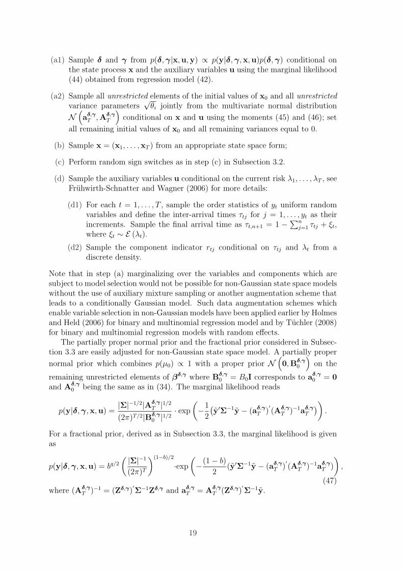
For these data, we were not able to estimate the model under the completely centeredparameterization as MCMC did not convergence. For this reason, we compare aparameterization where only the season is non-centered (Fruhwirth-Schnatter andWagner, 2006) under the priors θi ∼ G−1 (0.1, 0.001) , i = 1, 2, ±√θ3 ∼ N (0, 1)with a fully noncentered model with priors ±√θi ∼ N (0, 1) , i = 1, 2, 3. For bothparameterizations we assume that µ0 ∼ N (log(y1/e1), 1) = N (−9.0084, 1) and thatthe unknown initial values of the other components and the intervention effect followa standard normal prior distribution. We used 20000 iterations after a burn-in of5000 for each parameterization. As in Subsection 3.4.1, we observe much bettermixing behavior of the MCMC sampler under the non-centered parametrization,see Figure 7.
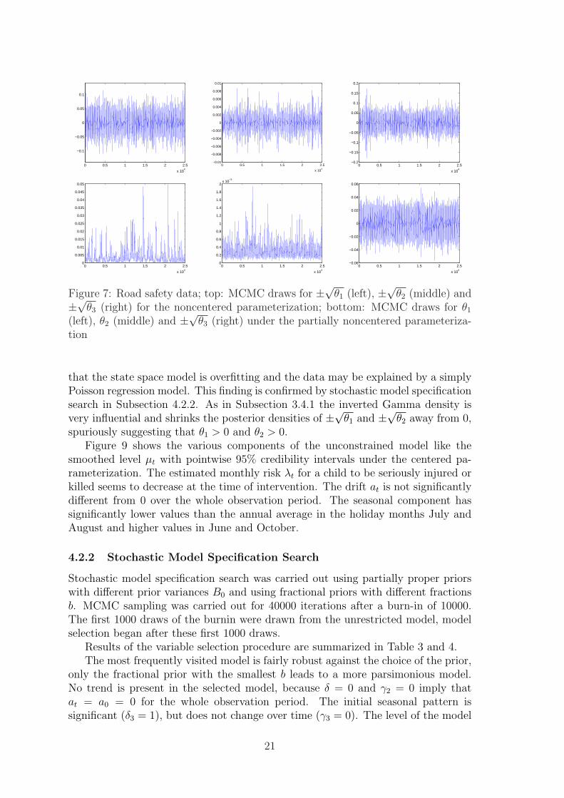
Figure 8 shows histograms of the MCMC draws for ±√θi, i = 1, . . . , 3 for bothparameterizations. For the noncentered parameterization with the normal prior theposterior of all parameters ±√θi, i = 1, . . . , 3 is clearly centered at 0, suggesting
1A shorter version of this time series ranging from 1987-2002 was analyzed in Fruhwirth-Schnatter and Wagner (2006).
20
0 0.5 1 1.5 2 2.5
x 104
−0.1
−0.05
0
0.05
0.1
0 0.5 1 1.5 2 2.5
x 104
−0.01
−0.008
−0.006
−0.004
−0.002
0
0.002
0.004
0.006
0.008
0.01
0 0.5 1 1.5 2 2.5
x 104
−0.2
−0.15
−0.1
−0.05
0
0.05
0.1
0.15
0.2
0 0.5 1 1.5 2 2.5
x 104
0
0.005
0.01
0.015
0.02
0.025
0.03
0.035
0.04
0.045
0.05
0 0.5 1 1.5 2 2.5
x 104
0
0.2
0.4
0.6
0.8
1
1.2
1.4
1.6
1.8
2x 10
−3
0 0.5 1 1.5 2 2.5
x 104
−0.06
−0.04
−0.02
0
0.02
0.04
0.06
Figure 7: Road safety data; top: MCMC draws for ±√θ1 (left), ±√θ2 (middle) and±√θ3 (right) for the noncentered parameterization; bottom: MCMC draws for θ1
(left), θ2 (middle) and ±√θ3 (right) under the partially noncentered parameteriza-tion
that the state space model is overfitting and the data may be explained by a simplyPoisson regression model. This finding is confirmed by stochastic model specificationsearch in Subsection 4.2.2. As in Subsection 3.4.1 the inverted Gamma density isvery influential and shrinks the posterior densities of ±√θ1 and ±√θ2 away from 0,spuriously suggesting that θ1 > 0 and θ2 > 0.
Figure 9 shows the various components of the unconstrained model like thesmoothed level µt with pointwise 95% credibility intervals under the centered pa-rameterization. The estimated monthly risk λt for a child to be seriously injured orkilled seems to decrease at the time of intervention. The drift at is not significantlydifferent from 0 over the whole observation period. The seasonal component hassignificantly lower values than the annual average in the holiday months July andAugust and higher values in June and October.
4.2.2 Stochastic Model Specification Search
Stochastic model specification search was carried out using partially proper priorswith different prior variances B0 and using fractional priors with different fractionsb. MCMC sampling was carried out for 40000 iterations after a burn-in of 10000.The first 1000 draws of the burnin were drawn from the unrestricted model, modelselection began after these first 1000 draws.
Results of the variable selection procedure are summarized in Table 3 and 4.The most frequently visited model is fairly robust against the choice of the prior,
only the fractional prior with the smallest b leads to a more parsimonious model.No trend is present in the selected model, because δ = 0 and γ2 = 0 imply thatat = a0 = 0 for the whole observation period. The initial seasonal pattern issignificant (δ3 = 1), but does not change over time (γ3 = 0). The level of the model
21
−0.1 −0.05 0 0.05 0.10
100
200
300
400
500
600
700
800
−6 −4 −2 0 2 4 6
x 10−3
0
400
800
1200
1600
2000
−0.1 −0.05 0 0.05 0.10
100
200
300
400
500
600
700
800
−0.2 −0.15 −0.1 −0.05 0 0.05 0.1 0.15 0.20
200
400
600
800
1000
1200
1400
1600
1800
−0.04 −0.02 0 0.02 0.040
500
1000
1500
2000
2500
−0.04 −0.03 −0.02 −0.01 0 0.01 0.02 0.03 0.040
100
200
300
400
500
600
700
800
900
Figure 8: Road safety data; histograms of the MCMC draws for ±√θ1 (left),±√θ2 (middle) and ±√θ3 (right); top: N (0, 1) prior for ±√θi, i = 1, 2, 3; bottom:G−1 (0.1, 0.001)-prior for θ1 and θ2, N (0, 1) prior for ±√θ3
(a)
1987 1989 1991 1993 1995 1997 1999 2001 2003 2005
1
2
3
4x 10
−4
(b)
1987 1989 1991 1993 1995 1997 1999 2001 2003 2005−10
−9.5
−9
−8.5
−8
−7.5
(c)
1987 1989 1991 1993 1995 1997 1999 2001 2003 2005−0.2
−0.15
−0.1
−0.05
0
0.05
0.1
0.15
0.2
(d)
Jan Feb Mar Apr May Jun Jul Aug Sep Oct Nov Dec−1.5
−1
−0.5
0
0.5
1
Figure 9: Road safety data; (a) posterior mean of the risk λt; posterior meansand point-wise 95% credible regions of (b) the level µt, (c) the drift at and (d) theseasonal component st in year 2005 under the centered parameterization
22

Table 3: Road safety data; the three most frequently visited models (among 40000MCMC iterations) for various prior distributions
prior δ δ3 δ4 γ1 γ2 γ3 frequencyp(µ0) ∝ 1, B0 = 1 0 1 1 0 0 0 37544
0 1 1 0 0 1 9370 1 1 1 0 0 611
p(µ0) ∝ 1, B0 = 100 0 1 1 0 0 0 348740 1 0 0 0 0 47430 1 1 0 0 1 125
b = 10−2 0 1 1 0 0 0 95950 1 1 0 0 1 41540 1 1 1 0 0 3414
b = 10−3 0 1 1 0 0 0 185281 1 0 0 0 0 40480 1 1 0 0 1 2686
b = 10−4 0 1 1 0 0 0 248711 1 0 0 0 0 47170 1 0 0 1 0 2514
b = 10−5 0 0 1 0 0 0 142980 0 1 0 0 1 78231 0 0 0 0 0 3991
is constant before and after intervention, because γ1 = 0. Most importantly, theintervention effect is significant, because δ4 = 1 is selected. Interestingly, the selectedmodel is no longer a state space model (γ1 = γ2 = γ3 = 0), but a simple Poissonregression model with monthly seasonal dummies and an intervention effect. Thisfinding is confirmed by the marginal likelihoods computed in Fruhwirth-Schnatterand Wagner (2008).
In Table 5 and Figure 10, we compare posterior inference for the interventioneffect for the unconstrained basic structural model and the model obtained by vari-able selection. We observe here an impressive gain of statistical efficiency for thisparameter of interest. For the unconstrained basic structural model, making thelevel dynamic before and after the intervention causes quite a loss of information,leading to an intervention effect that is not significant.
Table 4: Road safety data; marginal posterior probability of selecting each indicatortrend season intervention process variances
prior δ δ3 δ4 γ1 γ2 γ3
p(µ0) ∝ 1, B0 = 1 0.0047 1.0000 0.9798 0.0209 0.0005 0.0244p(µ0) ∝ 1, B0 = 100 0.0019 1.0000 0.8767 0.0042 0.0001 0.0035
b = 10−2 0.3140 1.0000 0.7769 0.2872 0.2767 0.3015b = 10−3 0.2152 1.0000 0.7094 0.1567 0.1576 0.1289b = 10−4 0.1563 1.0000 0.7196 0.0772 0.0963 0.0501b = 10−5 0.1753 0 0.5718 0.0734 0.0971 0.3514
23
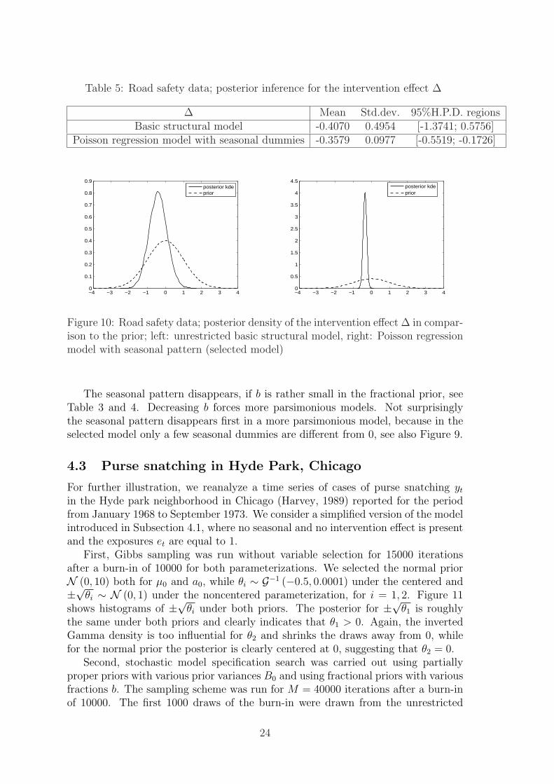
Table 5: Road safety data; posterior inference for the intervention effect ∆
∆ Mean Std.dev. 95%H.P.D. regionsBasic structural model -0.4070 0.4954 [-1.3741; 0.5756]
Poisson regression model with seasonal dummies -0.3579 0.0977 [-0.5519; -0.1726]
−4 −3 −2 −1 0 1 2 3 40
0.1
0.2
0.3
0.4
0.5
0.6
0.7
0.8
0.9
posterior kdeprior
−4 −3 −2 −1 0 1 2 3 40
0.5
1
1.5
2
2.5
3
3.5
4
4.5
posterior kdeprior
Figure 10: Road safety data; posterior density of the intervention effect ∆ in compar-ison to the prior; left: unrestricted basic structural model, right: Poisson regressionmodel with seasonal pattern (selected model)
The seasonal pattern disappears, if b is rather small in the fractional prior, seeTable 3 and 4. Decreasing b forces more parsimonious models. Not surprisinglythe seasonal pattern disappears first in a more parsimonious model, because in theselected model only a few seasonal dummies are different from 0, see also Figure 9.
4.3 Purse snatching in Hyde Park, Chicago
For further illustration, we reanalyze a time series of cases of purse snatching yt
in the Hyde park neighborhood in Chicago (Harvey, 1989) reported for the periodfrom January 1968 to September 1973. We consider a simplified version of the modelintroduced in Subsection 4.1, where no seasonal and no intervention effect is presentand the exposures et are equal to 1.
First, Gibbs sampling was run without variable selection for 15000 iterationsafter a burn-in of 10000 for both parameterizations. We selected the normal priorN (0, 10) both for µ0 and a0, while θi ∼ G−1 (−0.5, 0.0001) under the centered and±√θi ∼ N (0, 1) under the noncentered parameterization, for i = 1, 2. Figure 11shows histograms of ±√θi under both priors. The posterior for ±√θ1 is roughlythe same under both priors and clearly indicates that θ1 > 0. Again, the invertedGamma density is too influential for θ2 and shrinks the draws away from 0, whilefor the normal prior the posterior is clearly centered at 0, suggesting that θ2 = 0.
Second, stochastic model specification search was carried out using partiallyproper priors with various prior variances B0 and using fractional priors with variousfractions b. The sampling scheme was run for M = 40000 iterations after a burn-inof 10000. The first 1000 draws of the burn-in were drawn from the unrestricted
24

(a)
−0.5 −0.25 0 0.25 0.50
100
200
300
400
500
600
700
(b)
−0.1 −0.05 0 0.05 0.10
100
200
300
400
500
600
700
800
900
(c)
−0.5 −0.25 0 0.25 0.50
200
400
600
800
1000
1200
(d)
−0.1 −0.05 0 0.05 0.10
500
1000
1500
2000
2500
Figure 11: Purse snatching data; histograms for ±√θ1 (left) and ±√θ2 (right); top:N (0, 1) prior for ±√θ1 and ±√θ2; bottom: G−1 (−0.5, 0.0001)-prior for θ1 and θ2
Table 6: Purse snatching; the three most frequently visited models (among 40000MCMC iterations) for various prior distributions
δ γ1 γ2 B0 = 1 B0 = 100 b = 10−3 b = 10−4 b = 10−5
0 1 0 39436 39822 20944 32971 381351 1 0 442 166 8263 3705 9570 1 1 118 12 8110 3090 899
model, model selection began after these first 1000 draws.Results of the variable selection procedure are presented in Table 6 and 7. Model
selection is extremely robust to the prior choice and clearly picks a local level model.The drift disappears because δ = 0 and γ2 = 0 imply that at ≡ a0 = 0 for all t.This finding is confirms model selection by the marginal likelihoods in Fruhwirth-Schnatter and Wagner (2008).
Table 7: Purse snatching; marginal posterior probability of selecting each indicatorprior δ γ1 γ2
p(µ0) ∝ 1, B0 = 1 0.0112 1.0000 0.0031p(µ0) ∝ 1, B0 = 100 0.0042 1.0000 0.0003
b = 10−3 0.2698 1.0000 0.2737b = 10−4 0.0985 1.0000 0.0831b = 10−5 0.0227 1.0000 0.0242
25

5 Concluding remarks
The model space MCMC approach discussed in this paper could be easily adaptedto other state space models. Auxiliary mixture sampling as discussed in Fruhwirth-Schnatter and Fruhwirth (2007), for instance, allows to consider state space mod-elling of binary and categorical time series. Another important extension is searchingfor fixed and time-varying coefficients in a regression model.
A couple of modifications of our approach are worth being considered. First, theuniform prior over all models may be substituted by a more flexible prior which isobtained by assuming that the prior occurrence of δi = 1 and γi = 1 is different:
Pr(δi = 1|αδ) = αδ, Pr(γi = 1|αγ) = αγ.
In this prior, αδ and αγ may be chosen as fixed values, if prior information on theoccurrence probabilities is available. If this is not the case, a hyperprior may be puton αδ and αγ as in Smith and Kohn (2002) and Fruhwirth-Schnatter and Tuchler(2008). If both hyperparameters αδ and αγ are iid Uniform on [0,1], then
p(δ, γ) = B(1 +∑
i
I{δi=1}, 1 +∑
i
I{δi=0})B(1 +∑
i
I{γi=1}, 1 +∑
i
I{γi=0}),
where B(·, ·) is the Beta function. This prior leads to a uniform distribution overmodel size and outperforms the uniform prior over all models in variable selectionfor large regression models, see Ley and Steel (2007). In our applications, wheremodel size is small, posterior inference under both priors is virtually the same.
Second, sampling the indicators could be modified. In our MCMC schemes,the indicators (δ, γ) are sampled jointly from the discrete posterior p(δ,γ|x,y) byevaluating the right hand side of (25) for all combinations of indicators at eachsweep of the sampler. This multi-move sampling is rather time-consuming and maybe substituted single-move sampling, i.e. sampling recursively from p(δj|δ−j, γ,x,y)and p(γj|γ−j, δ,x,y).
An open issue of our approach is the influence the prior on the initial valuesand the process variances exercises on final model selection. We demonstrated thatthe normal prior put on the signed square root of the process variances is far lessinfluential than the usual inverted Gamma for the process variances themselves.The sensitivity analysis carried out for all of our case studies revealed a surprisingrobustness of the finally selected model against variation in the normal prior. Aconcise statement which prior scale leads to model consistency in the sense of Casella,Giron, Martınez, and Moreno (2006), however, is far beyond the scope of the presentpaper.
References
Carter, C. K. and R. Kohn (1994). On Gibbs sampling for state space models.Biometrika 81, 541–553.
Casella, G., F. J. Giron, M. L. Martınez, and E. Moreno (2006). Consistency ofBayesian procedures for variable selection. Research Report.
26

Chen, Z. and D. Dunson (2003). Random effects selection in linear mixed models.Biometrics 59, 762–769.
Chib, S. (1995). Marginal likelihood from the Gibbs output. Journal of the AmericanStatistical Association 90, 1313–1321.
De Jong, P. and N. Shephard (1995). The simulation smoother for time seriesmodels. Biometrika 82, 339–350.
Durbin, J. and S. J. Koopman (2000). Time series analysis of non-Gaussian observa-tions based on state space models from both classical and Bayesian perspectives.Journal of the Royal Statistical Society, Ser. B 62, 3–56.
Fernandez, C., E. Ley, and M. F. J. Steel (2001). Benchmark priors for Bayesianmodel averaging. Journal of Econometrics 100, 381–427.
Fruhwirth-Schnatter, S. (1994). Data augmentation and dynamic linear models.Journal of Time Series Analysis 15, 183–202.
Fruhwirth-Schnatter, S. (1995). Bayesian model discrimination and Bayes factorsfor linear Gaussian state space models. Journal of the Royal Statistical Society,Ser. B 57, 237–246.
Fruhwirth-Schnatter, S. (2001). Fully Bayesian analysis of switching Gaussian statespace models. Annals of the Institute of Statistical Mathematics 53, 31–49.
Fruhwirth-Schnatter, S. and R. Fruhwirth (2007). Auxiliary mixture sampling withapplications to logistic models. Computational Statistics and Data Analysis 51,3509–3528.
Fruhwirth-Schnatter, S., R. Fruhwirth, L. Held, and H. Rue (2007). Improved aux-iliary mixture sampling for hierarchical models of non-Gaussian data. IFAS Re-search Report 2007-25, http://ifas.jku.at, Johannes Kepler University Linz.
Fruhwirth-Schnatter, S. and R. Tuchler (2008). Bayesian parsimonious covarianceestimation for hierarchical linear mixed models. Statistics and Computing , 1–13.
Fruhwirth-Schnatter, S. and H. Wagner (2006). Auxiliary mixture sampling forparameter-driven models of time series of small counts with applications to statespace modelling. Biometrika 93, 827–841.
Fruhwirth-Schnatter, S. and H. Wagner (2008). Marginal likelihoods for non-Gaussian models using auxiliary mixture sampling. Computational Statistics andData Analysis , accepted for publication.
George, E. I. and R. McCulloch (1993). Variable selection via Gibbs sampling.Journal of the American Statistical Association 88, 881–889.
George, E. I. and R. McCulloch (1997). Approaches for Bayesian variable selection.Statistica Sinica 7, 339–373.
27

Green, P. J. (1995). Reversible jump Markov chain Monte Carlo computation andBayesian model determination. Biometrika 82, 711–732.
Harvey, A. C. (1989). Forecasting, Structural Time Series Models and the KalmanFilter. Cambridge: Cambridge University Press.
Harvey, A. C. and J. Durbin (1986). The effects of seat belt legislation on Britishroad casualties: A case study in structural time series modelling. Journal of theRoyal Statistical Society, Ser. A 149, 187–227.
Holmes, C. C. and L. Held (2006). Bayesian auxiliary variable models for binaryand multinomial regression. Bayesian Analysis 1, 145–168.
Jeffreys, S. H. (1948). Theory of Probability (2 ed.). Oxford: Clarendon.
Ley, E. and M. F. J. Steel (2007). On the effect of prior assumptions in Bayesianmodel averaging with applications to growth regression. Technical Report CRiSMWorking Paper 07-08, University of Warwick.
O’Hagan, A. (1995). Fractional Bayes factors for model comparison (Disc: p118-138). Journal of the Royal Statistical Society, Ser. B 57, 99–118.
Shively, T. S. and R. Kohn (1997). A Bayesian approach to model selection instochastic coefficient regression models and structural time series models. Journalof Econometrics 76, 39–52.
Smith, M. and R. Kohn (2002). Parsimonious covariance matrix estimation forlongitudinal data. Journal of the American Statistical Association 97, 1141–1153.
Tuchler, R. (2008). Bayesian variable selection for logistic models using auxiliarymixture sampling. Journal of Computational and Graphical Statistics 17, 76–94.
Zellner, A. (1971). An Introduction to Bayesian Inference in Econometrics. NewYork: Wiley.
28