Embed Size (px)
Citation preview

In: Advances in Systems Engineering Research ISBN: 978-1-62948-310-8
Editors: Elena Fermi and Adam Lamberti © 2013 Nova Science Publishers, Inc.
Chapter 3
SIMULATION OF THE SEPARATION OF INDUSTRIALLY
IMPORTANT HYDROCARBON MIXTURES BY
DIFFERENT DISTILLATION TECHNIQUES
USING MATHEMATICA©
Housam Binous1 and Ahmed Bellagi
2
1Department of Chemical Engineering, King Fahd University of Petroleum & Minerals,
KSA 2Département de Génie Energétique (Energy Engineering Department), Ecole Nationale
d’Ingénieurs de Monastir, University of Monastir, Tunisia
ABSTRACT
In this chapter the simulation of several case studies for the separation by distillation
of various industrially relevant hydrocarbon mixtures are worked out. Different
techniques used to separate the complex mixtures are illustrated: classical column train
and enhanced distillation (extractive and reactive).
This chapter is aimed primarily at chemical engineering students. But the
information presented might be also useful for postgraduate and PhD students as well as
professional engineers.
An important objective of this chapter is to show how these rather complex
separations can be handled with great pedagogical benefits using the computer algebra
Mathematica©, a general purpose solver, not chemical engineering specific. Simulation
results are compared to those obtained using the flow-sheeting software Aspen-HYSYS®.
Five case studies are worked out: the separation of natural gas liquids (NGL), the
fractionation of a C4 cut to separate 1,3-butadiene with furfural as entrainer, the
production of MTBE from i-butene and methanol, the reverse process: production of i-
butene and methanol by the decomposition of methyl tert-butyl ether (MTBE), and the
equilibrium-limited metathesis of cis-2-pentene to cis-2-butene and cis-2-hexene.
For every case complete information is given such that it can be easily reproduced
with the process simulator and/or alternatively worked out using the relevant
Mathematica© programs available at http://demonstrations.wolfram.com.
The exclusive license for this PDF is limited to personal website use only. No part of this digital document may be reproduced, stored in a retrieval system or transmitted commercially in any form or by any means. The publisher has taken reasonable care in the preparation of this digital document, but makes no expressed or implied warranty of any kind and assumes no responsibility for any errors or omissions. No liability is assumed for incidental or consequential damages in connection with or arising out of information contained herein. This digital document is sold with the clear understanding that the publisher is not engaged in rendering legal, medical or any other professional services.

Housam Binous and Ahmed Bellagi 48
Keywords: Enhanced distillation, NGL train, Extractive distillation, Reactive distillation,
Numerical simulations, Mathematica©, Aspen HYSYS®
INTRODUCTION
Distillation is a reliable separation technique, and remains often the most efficient
fractionation method. The ubiquity of the distillation installations in the gas, oil and
petrochemical industry makes it indeed be considered as the “workhorse” separation process
in this field.
In this chapter, the fractionation by different distillation techniques of various industrially
relevant hydrocarbon mixtures is investigated. Mathematical modeling and numerical
simulation are our exploration tools. The objective is to illustrate different distillation
techniques used to separate complex mixtures: classical column train, and enhanced
distillation (extractive and reactive).
Five case studies illustrating different separation distillation techniques are worked out.
The first case study deals with the separation of natural gas liquids (NGLs), a mixture of
light hydrocarbons (ethane, propane, butane, pentane, hexane and heptanes). The raw NGLs
mixture is separated using a sequence of distillation columns in which the desired
hydrocarbons are gradually isolated.
The second case study is the extraction of 1,3-butadiene from a C4-cut using extractive
distillation with furfural as entrainer.
The remaining three cases are dedicated to the simulation of reactive distillation columns
for:
The production of methyl tert-butyl ether (MTBE) from i-butene and methanol,
The production of i-butene by the reverse process of decomposition of MTBE,
The equilibrium-limited metathesis of cis-2-pentene to cis-2-butene and cis-2-
hexene.
The various case studies are first worked out using the well-known flow-sheeting
software Aspen-HYSYS®. It is an important objective of this chapter however to show how
these rather complex separations can also be handled with great pedagogical benefits using
the more accessible computer algebra Mathematica©, a general purpose solver, not chemical
engineering specific.
This approach is particularly suitable for undergraduate students, as at this level of
chemical engineering formation, the synthetic pedagogical approach is more effective and can
be very rewarding. The student builds all from starch and has to elaborate by himself a model
for the process under investigation. During this step of model development, one learns a lot
about equations of state, departure functions, activity models, MESH equations…
By integrating the basic mathematical functions with the powerful and easy-to-use
programming language Mathematica©, it is possible to handle processes that would be
extremely tedious to encode in traditional programming environments. Using this powerful
tool let the student concentrate on the very process he/she is investigating and enhances
dramatically the overall understanding of his/her project. As illustrated in this chapter various
Simulation of the Separation of Industrially Important Hydrocarbon Mixtures ... 49
process alternatives can easily be probed (integration of the pressure drop in the stages, taking
account of the non ideal efficiency of the plates, trying different solvents, etc.).
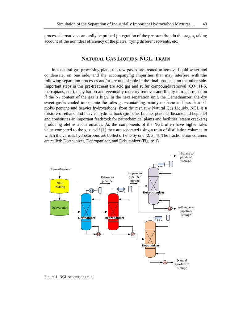
NATURAL GAS LIQUIDS, NGL, TRAIN
In a natural gas processing plant, the raw gas is pre-treated to remove liquid water and
condensate, on one side, and the accompanying impurities that may interfere with the
following separation processes and/or are undesirable in the final products, on the other side.
Important steps in this pre-treatment are acid gas and sulfur compounds removal (CO2, H2S,
mercaptans, etc.), dehydration and eventually mercury removal and finally nitrogen rejection
if the N2 content of the gas is high. In the next separation unit, the Demethanizer, the dry
sweet gas is cooled to separate the sales gas−containing mainly methane and less than 0.1
mol% pentane and heavier hydrocarbons−from the rest, raw Natural Gas Liquids. NGL is a
mixture of ethane and heavier hydrocarbons (propane, butane, pentane, hexane and heptane)
and constitutes an important feedstock for petrochemical plants and facilities (steam crackers)
producing olefins and aromatics. As the components of the NGL often have higher sales
value compared to the gas itself [1] they are separated using a train of distillation columns in
which the various hydrocarbons are boiled off one by one [2, 3, 4]. The fractionation columns
are called: Deethanizer, Depropanizer, and Debutanizer (Figure 1).
Figure 1. NGL separation train.
Demethanizer
Dehydration
NGL
treating
Deethanizer Depropanizer
Ethane to
pipeline
Propane to
pipeline/
storage
Natural
gasoline to
storage
Debutanizer
n-Butane to
pipeline/
storage
i-Butane to
pipeline/
storage
Deisobutanizer
Housam Binous and Ahmed Bellagi 50
This first case study deals with the simulation of an NGL train. Raw NGL is to be
separated in almost pure ethane, i-butane, n-butane, and a mixture composed of propane and
the rest of the dissolved ethane. The bottom product of the last fractionation unit is natural
gasoline.
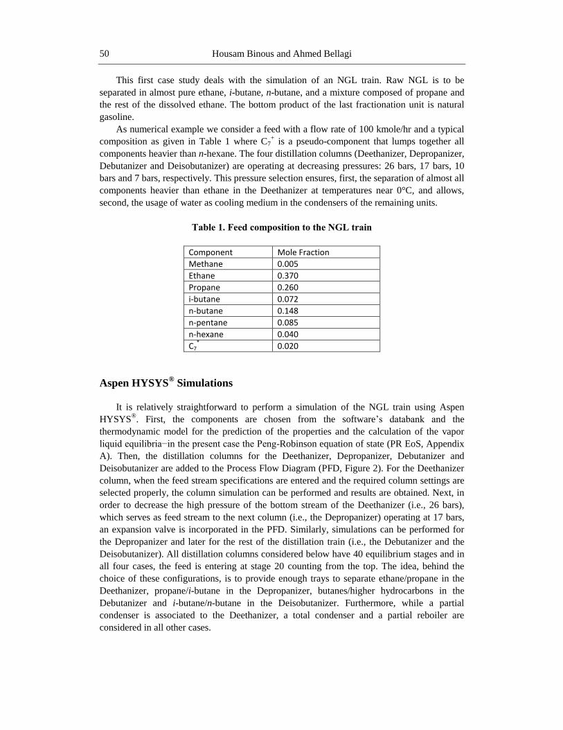
As numerical example we consider a feed with a flow rate of 100 kmole/hr and a typical
composition as given in Table 1 where C7+ is a pseudo-component that lumps together all
components heavier than n-hexane. The four distillation columns (Deethanizer, Depropanizer,
Debutanizer and Deisobutanizer) are operating at decreasing pressures: 26 bars, 17 bars, 10
bars and 7 bars, respectively. This pressure selection ensures, first, the separation of almost all
components heavier than ethane in the Deethanizer at temperatures near 0°C, and allows,
second, the usage of water as cooling medium in the condensers of the remaining units.
Table 1. Feed composition to the NGL train
Component Mole Fraction
Methane 0.005
Ethane 0.370
Propane 0.260
i-butane 0.072
n-butane 0.148
n-pentane 0.085
n-hexane 0.040
C7* 0.020
Aspen HYSYS® Simulations
It is relatively straightforward to perform a simulation of the NGL train using Aspen
HYSYS®. First, the components are chosen from the software’s databank and the
thermodynamic model for the prediction of the properties and the calculation of the vapor
liquid equilibria−in the present case the Peng-Robinson equation of state (PR EoS, Appendix
A). Then, the distillation columns for the Deethanizer, Depropanizer, Debutanizer and
Deisobutanizer are added to the Process Flow Diagram (PFD, Figure 2). For the Deethanizer
column, when the feed stream specifications are entered and the required column settings are
selected properly, the column simulation can be performed and results are obtained. Next, in
order to decrease the high pressure of the bottom stream of the Deethanizer (i.e., 26 bars),
which serves as feed stream to the next column (i.e., the Depropanizer) operating at 17 bars,
an expansion valve is incorporated in the PFD. Similarly, simulations can be performed for
the Depropanizer and later for the rest of the distillation train (i.e., the Debutanizer and the
Deisobutanizer). All distillation columns considered below have 40 equilibrium stages and in
all four cases, the feed is entering at stage 20 counting from the top. The idea, behind the
choice of these configurations, is to provide enough trays to separate ethane/propane in the
Deethanizer, propane/i-butane in the Depropanizer, butanes/higher hydrocarbons in the
Debutanizer and i-butane/n-butane in the Deisobutanizer. Furthermore, while a partial
condenser is associated to the Deethanizer, a total condenser and a partial reboiler are
considered in all other cases.
Simulation of the Separation of Industrially Important Hydrocarbon Mixtures ... 51
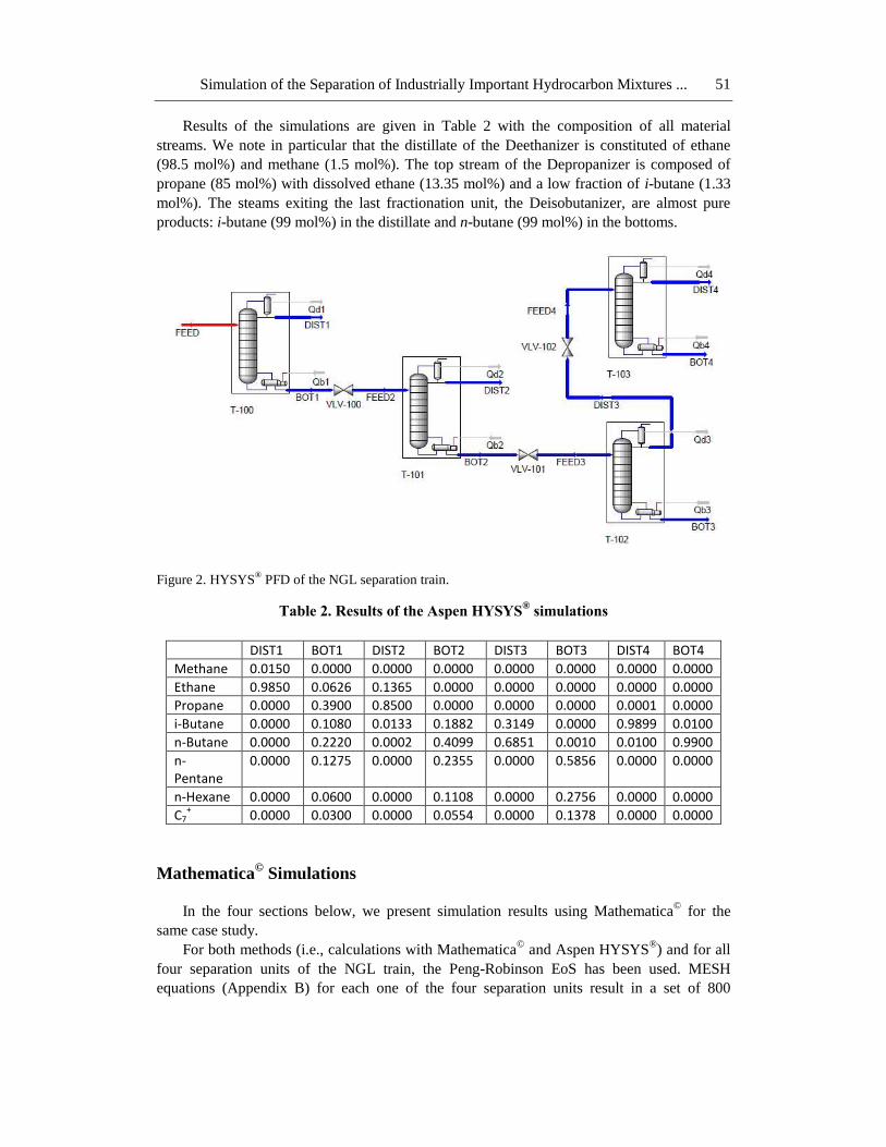
Results of the simulations are given in Table 2 with the composition of all material
streams. We note in particular that the distillate of the Deethanizer is constituted of ethane
(98.5 mol%) and methane (1.5 mol%). The top stream of the Depropanizer is composed of
propane (85 mol%) with dissolved ethane (13.35 mol%) and a low fraction of i-butane (1.33
mol%). The steams exiting the last fractionation unit, the Deisobutanizer, are almost pure
products: i-butane (99 mol%) in the distillate and n-butane (99 mol%) in the bottoms.
Figure 2. HYSYS® PFD of the NGL separation train.
Table 2. Results of the Aspen HYSYS® simulations
DIST1 BOT1 DIST2 BOT2 DIST3 BOT3 DIST4 BOT4
Methane 0.0150 0.0000 0.0000 0.0000 0.0000 0.0000 0.0000 0.0000
Ethane 0.9850 0.0626 0.1365 0.0000 0.0000 0.0000 0.0000 0.0000
Propane 0.0000 0.3900 0.8500 0.0000 0.0000 0.0000 0.0001 0.0000
i-Butane 0.0000 0.1080 0.0133 0.1882 0.3149 0.0000 0.9899 0.0100
n-Butane 0.0000 0.2220 0.0002 0.4099 0.6851 0.0010 0.0100 0.9900
n-Pentane
0.0000 0.1275 0.0000 0.2355 0.0000 0.5856 0.0000 0.0000
n-Hexane 0.0000 0.0600 0.0000 0.1108 0.0000 0.2756 0.0000 0.0000
C7+ 0.0000 0.0300 0.0000 0.0554 0.0000 0.1378 0.0000 0.0000
Mathematica©
Simulations
In the four sections below, we present simulation results using Mathematica© for the
same case study.
For both methods (i.e., calculations with Mathematica© and Aspen HYSYS
®) and for all
four separation units of the NGL train, the Peng-Robinson EoS has been used. MESH
equations (Appendix B) for each one of the four separation units result in a set of 800
Housam Binous and Ahmed Bellagi 52
nonlinear algebraic equations, which are readily solved using Mathematica© in less than five
minutes with an Intel® Core
™ 2 Duo CPU T9600 2.80 GHz RAM 4 GB.
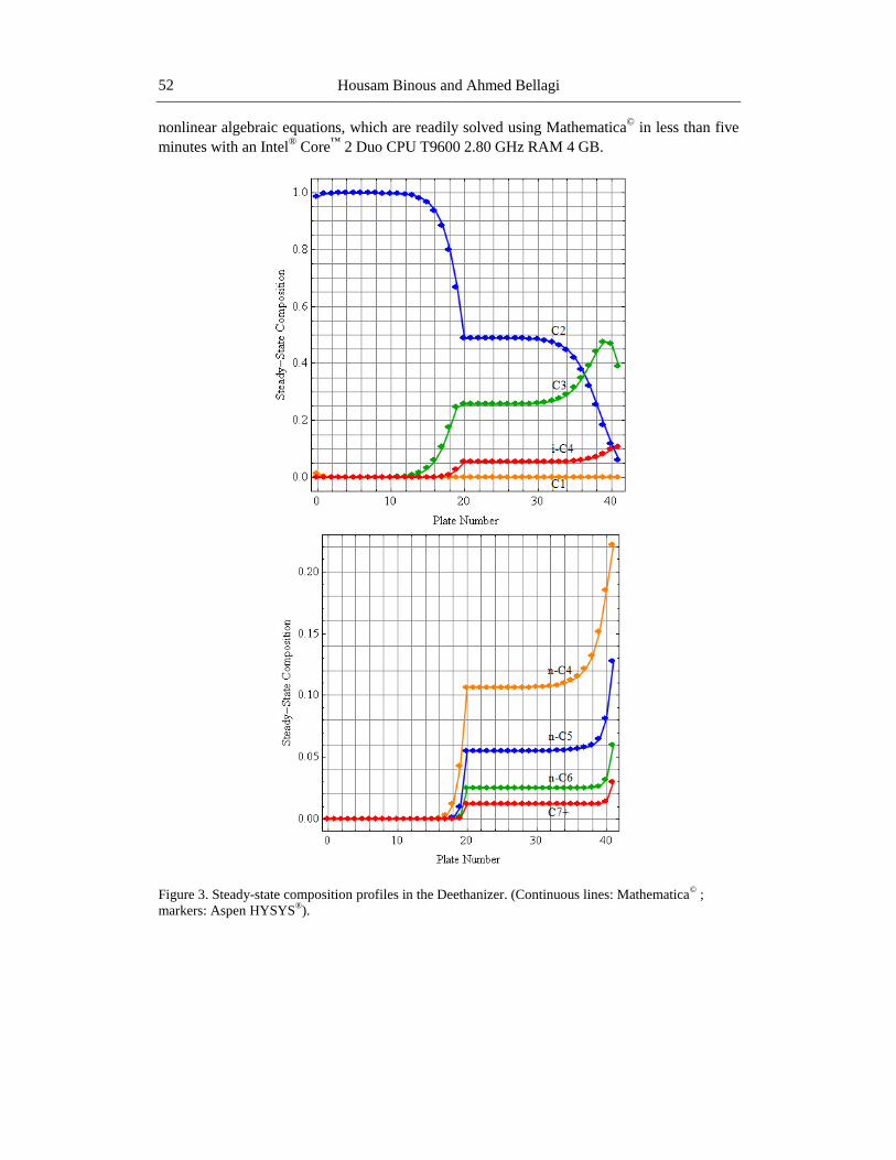
Figure 3. Steady-state composition profiles in the Deethanizer. (Continuous lines: Mathematica© ;
markers: Aspen HYSYS®).
Simulation of the Separation of Industrially Important Hydrocarbon Mixtures ... 53
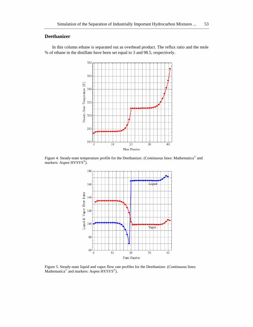
Deethanizer
In this column ethane is separated out as overhead product. The reflux ratio and the mole
% of ethane in the distillate have been set equal to 3 and 98.5, respectively.
Figure 4. Steady-state temperature profile for the Deethanizer. (Continuous lines: Mathematica© and
markers: Aspen HYSYS®).
Figure 5. Steady-state liquid and vapor flow rate profiles for the Deethanizer. (Continuous lines:
Mathematica© and markers: Aspen HYSYS
®).

Housam Binous and Ahmed Bellagi 54
Figures 3-5 show the steady-state composition and temperature profiles as well as the
liquid and vapor flow rates in the column. The distillate product has a flow rate of 33.33
kmole/hr and contains: 1.5 mol% methane and 98.5 mol% ethane. The bottom product from
Deethanizer enters into the next column (i.e., the Depropanizer) with a flow rate equal to
66.66 kmole/hr and the following composition: 6.25 mol% ethane, 39.0 mol% propane, 10.8
mol% i-butane, 22.2 mol% n-butane, 12.75 mol% n-pentane, 6.0 mol% n-hexane and 3 mol%
C7+. The cooling and heating duties of the condenser and reboiler are 1.167 10
6 and 1.542 10
6
kJ/hr, respectively.
We note from Figures 3-5 also that the results of our Mathematica©
simulations
(continuous lines) match perfectly the results obtained with Aspen HYSYS® (markers). This
is true for the composition profiles of all of the constituents in the column (Figure 3) as well
as for the temperature evolution (Figure 4) and the total molar flow rates of vapor and liquid
(Figure 5).
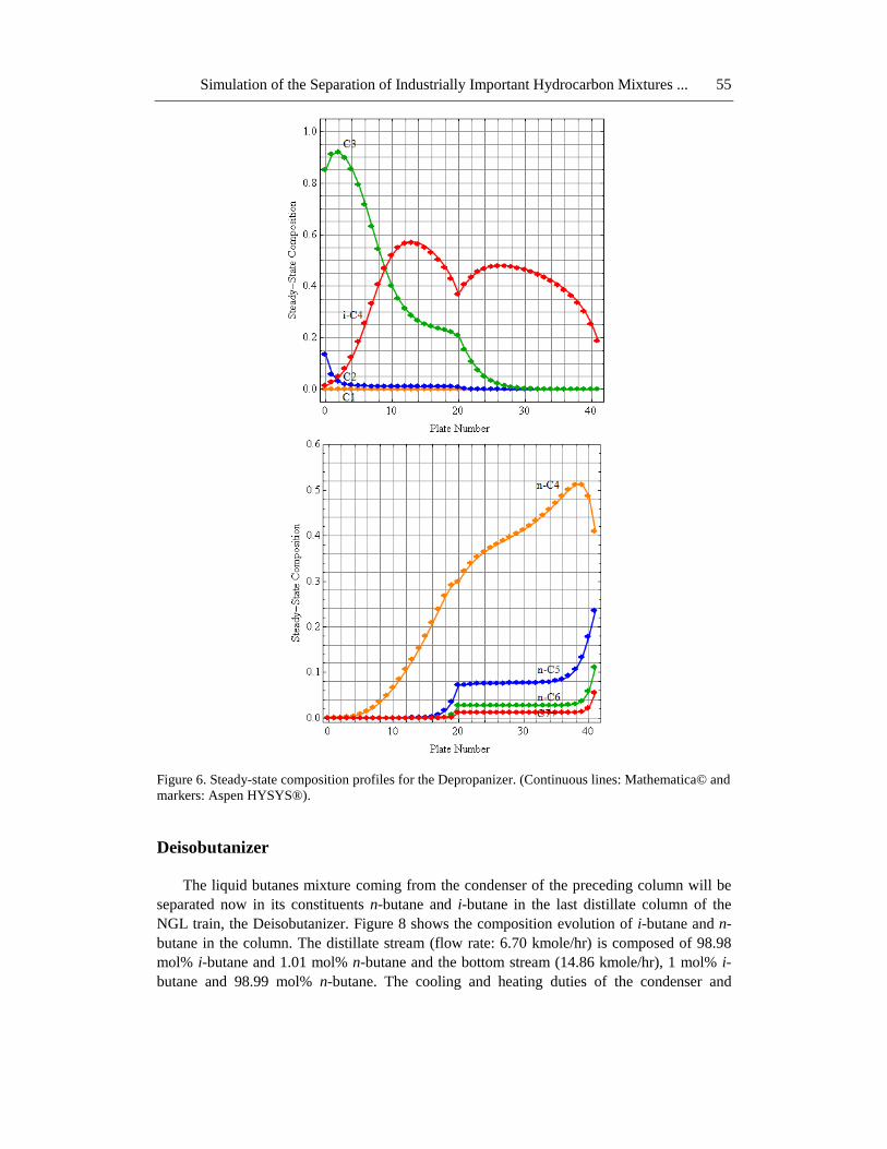
Depropanizer
The bottom stream of the Deethanizer serves as feed stream to the Depropanizer. The
overhead product of this column is propane rich and is condensed in the condenser. The
reflux ratio and the mol% of propane in the distillate have been set equal to 5 and 85.0,
respectively. Figure 6 shows the steady-state composition profile of this distillation column.
The distillate stream has a flow rate equal to 30.58 kmole/hr and contains: 13.64 mol%
ethane, 85 mol% propane and 1.33 mol% i-butane. The bottom stream has a flow rate equal to
36.07 kmole/hr and is composed of 18.82 mol% i-butane, 41 mol% n-butane, 23.55 mol% n-
pentane, 11.08 mol% n-hexane and 5.55 mol% C7+. The cooling and heating duties of the
condenser and reboiler are 2.429 106 and 2.348 10
6 kJ/hr, respectively. Again, perfect
agreement was obtained with Aspen HYSYS®, just as in the case of the Deethanizer. For
simplicity, only compositions profiles comparison (continuous lines for Mathematica© and
markers for HYSYS results) are shown in Figure 6.
Debutanizer
The stream exiting the Depropanizer reboiler serves as feed stream, after reduction of its
pressure, to the Debutanizer. The reflux ratio and the mol% of n-butane in the residue have
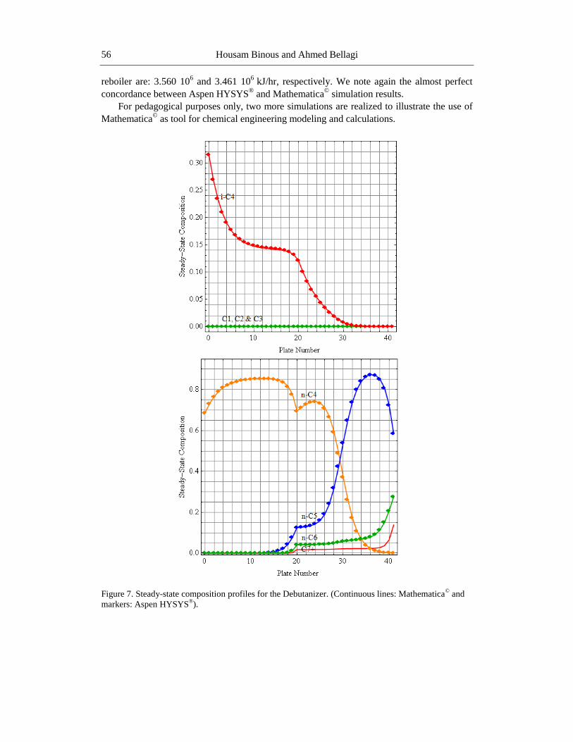
been set to 5 and 0.1, respectively. In Figure 7 the steady-state composition profiles of all
constituents inside this distillation column are represented. i-butane and n-butane are
separated out as overhead product. The distillate stream has a flow rate equal to 21.56
kmole/hr and contains a butane mixture with 31.48 mol% i-butane and 68.51 mol% n-butane.
The bottom stream with a flow rate of 36.07 kmole/hr is composed of 58.56 mol% n-pentane,
27.55 mol% n-hexane and 13.87 mol% C7+. The cooling and heating duties of the condenser
and reboiler are found to be 2.200 106 and 2.070 10
6 kJ/hr, respectively. Once more, perfect
agreement was obtained with Aspen HYSYS® results.
Simulation of the Separation of Industrially Important Hydrocarbon Mixtures ... 55
Figure 6. Steady-state composition profiles for the Depropanizer. (Continuous lines: Mathematica© and
markers: Aspen HYSYS®).
Deisobutanizer
The liquid butanes mixture coming from the condenser of the preceding column will be
separated now in its constituents n-butane and i-butane in the last distillate column of the
NGL train, the Deisobutanizer. Figure 8 shows the composition evolution of i-butane and n-
butane in the column. The distillate stream (flow rate: 6.70 kmole/hr) is composed of 98.98
mol% i-butane and 1.01 mol% n-butane and the bottom stream (14.86 kmole/hr), 1 mol% i-
butane and 98.99 mol% n-butane. The cooling and heating duties of the condenser and
Housam Binous and Ahmed Bellagi 56
reboiler are: 3.560 106 and 3.461 10
6 kJ/hr, respectively. We note again the almost perfect
concordance between Aspen HYSYS® and Mathematica
© simulation results.
For pedagogical purposes only, two more simulations are realized to illustrate the use of
Mathematica© as tool for chemical engineering modeling and calculations.
Figure 7. Steady-state composition profiles for the Debutanizer. (Continuous lines: Mathematica© and
markers: Aspen HYSYS®).
Simulation of the Separation of Industrially Important Hydrocarbon Mixtures ... 57
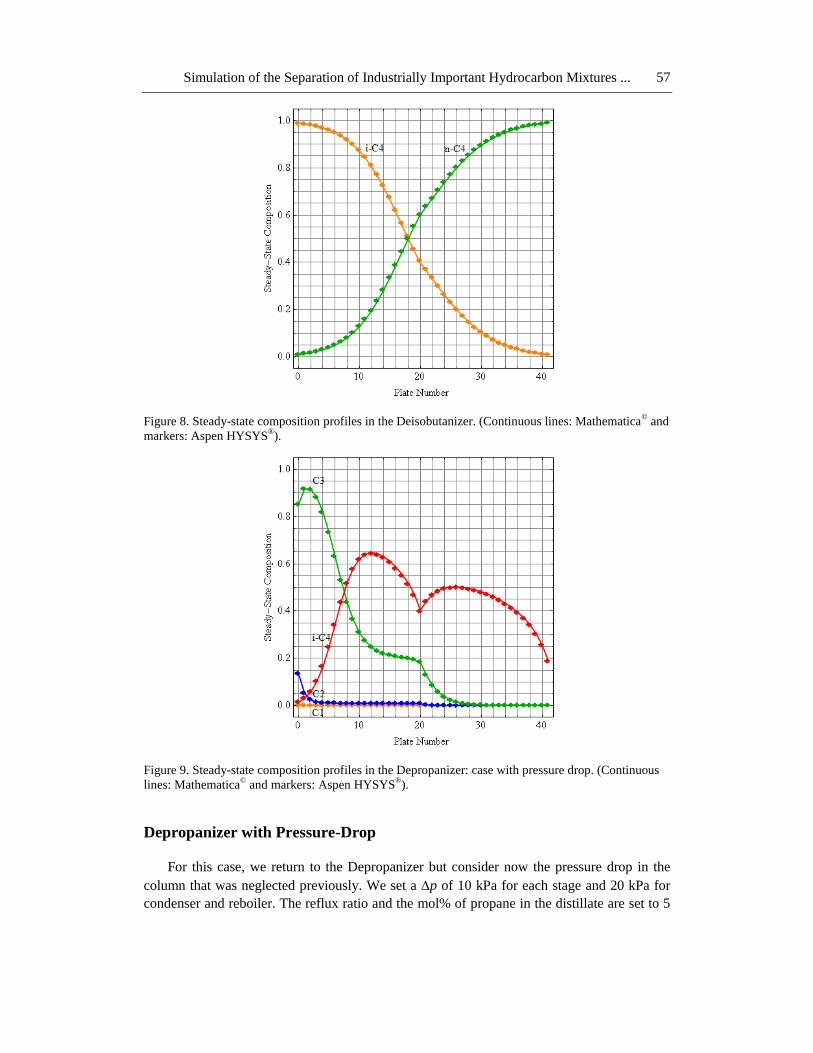
Figure 8. Steady-state composition profiles in the Deisobutanizer. (Continuous lines: Mathematica© and
markers: Aspen HYSYS®).
Figure 9. Steady-state composition profiles in the Depropanizer: case with pressure drop. (Continuous
lines: Mathematica© and markers: Aspen HYSYS
®).
Depropanizer with Pressure-Drop
For this case, we return to the Depropanizer but consider now the pressure drop in the
column that was neglected previously. We set a p of 10 kPa for each stage and 20 kPa for
condenser and reboiler. The reflux ratio and the mol% of propane in the distillate are set to 5
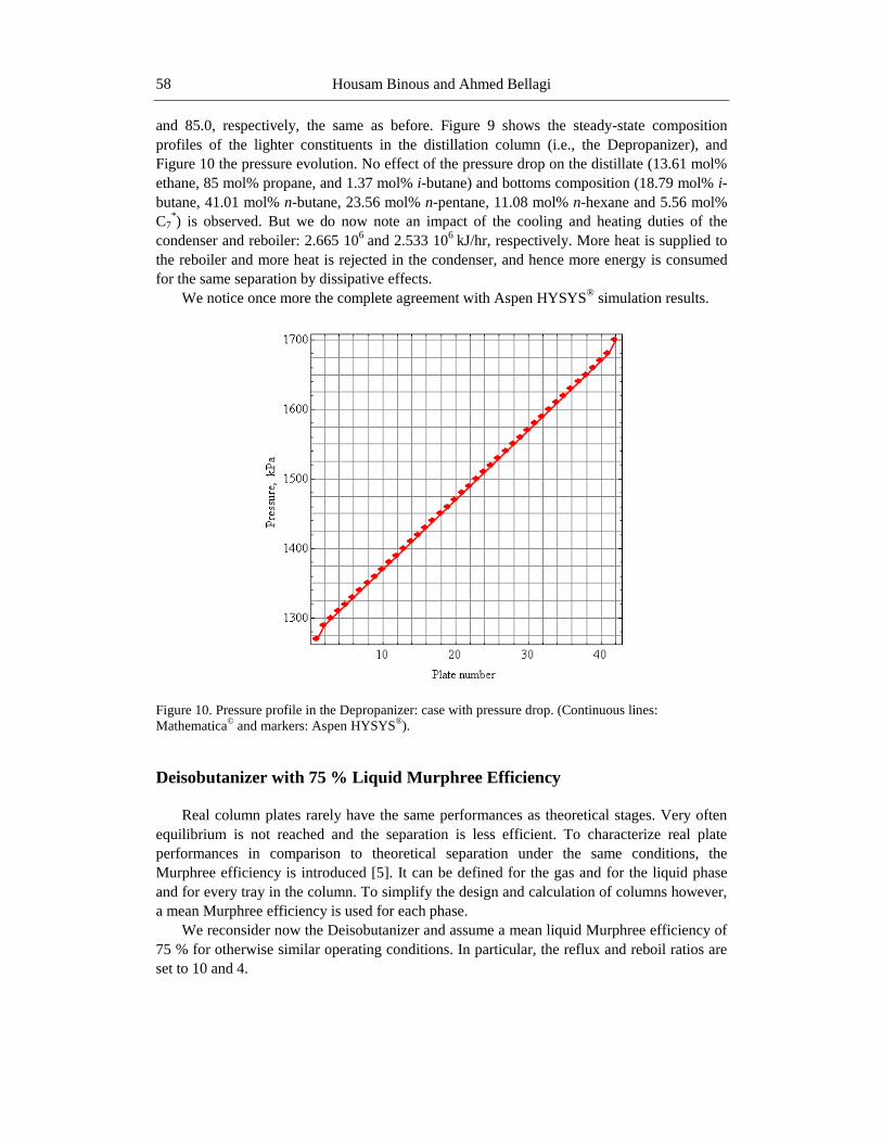
Housam Binous and Ahmed Bellagi 58
and 85.0, respectively, the same as before. Figure 9 shows the steady-state composition
profiles of the lighter constituents in the distillation column (i.e., the Depropanizer), and
Figure 10 the pressure evolution. No effect of the pressure drop on the distillate (13.61 mol%
ethane, 85 mol% propane, and 1.37 mol% i-butane) and bottoms composition (18.79 mol% i-
butane, 41.01 mol% n-butane, 23.56 mol% n-pentane, 11.08 mol% n-hexane and 5.56 mol%
C7*) is observed. But we do now note an impact of the cooling and heating duties of the
condenser and reboiler: 2.665 106
and 2.533 106
kJ/hr, respectively. More heat is supplied to
the reboiler and more heat is rejected in the condenser, and hence more energy is consumed
for the same separation by dissipative effects.
We notice once more the complete agreement with Aspen HYSYS® simulation results.
Figure 10. Pressure profile in the Depropanizer: case with pressure drop. (Continuous lines:
Mathematica© and markers: Aspen HYSYS
®).
Deisobutanizer with 75 % Liquid Murphree Efficiency
Real column plates rarely have the same performances as theoretical stages. Very often
equilibrium is not reached and the separation is less efficient. To characterize real plate
performances in comparison to theoretical separation under the same conditions, the
Murphree efficiency is introduced [5]. It can be defined for the gas and for the liquid phase
and for every tray in the column. To simplify the design and calculation of columns however,
a mean Murphree efficiency is used for each phase.
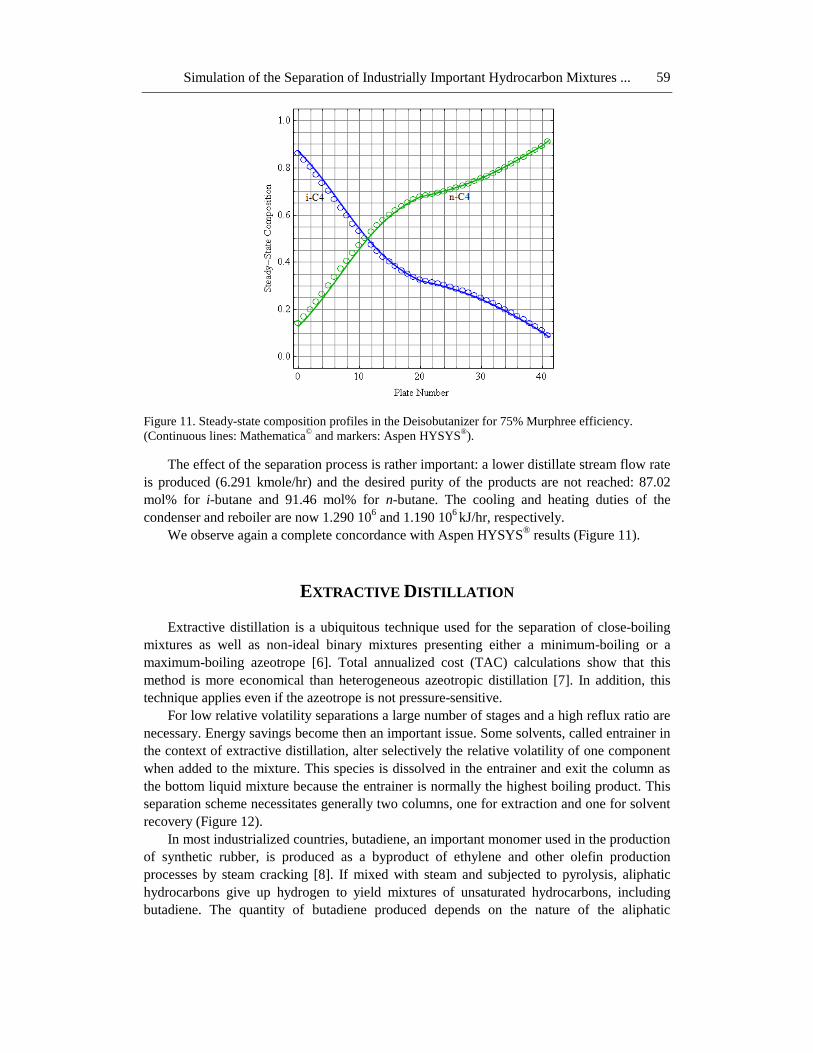
We reconsider now the Deisobutanizer and assume a mean liquid Murphree efficiency of
75 % for otherwise similar operating conditions. In particular, the reflux and reboil ratios are
set to 10 and 4.
Simulation of the Separation of Industrially Important Hydrocarbon Mixtures ... 59
Figure 11. Steady-state composition profiles in the Deisobutanizer for 75% Murphree efficiency.
(Continuous lines: Mathematica© and markers: Aspen HYSYS
®).
The effect of the separation process is rather important: a lower distillate stream flow rate
is produced (6.291 kmole/hr) and the desired purity of the products are not reached: 87.02
mol% for i-butane and 91.46 mol% for n-butane. The cooling and heating duties of the
condenser and reboiler are now 1.290 106 and 1.190 10
6 kJ/hr, respectively.
We observe again a complete concordance with Aspen HYSYS® results (Figure 11).
EXTRACTIVE DISTILLATION
Extractive distillation is a ubiquitous technique used for the separation of close-boiling
mixtures as well as non-ideal binary mixtures presenting either a minimum-boiling or a
maximum-boiling azeotrope [6]. Total annualized cost (TAC) calculations show that this
method is more economical than heterogeneous azeotropic distillation [7]. In addition, this
technique applies even if the azeotrope is not pressure-sensitive.
For low relative volatility separations a large number of stages and a high reflux ratio are
necessary. Energy savings become then an important issue. Some solvents, called entrainer in
the context of extractive distillation, alter selectively the relative volatility of one component
when added to the mixture. This species is dissolved in the entrainer and exit the column as
the bottom liquid mixture because the entrainer is normally the highest boiling product. This
separation scheme necessitates generally two columns, one for extraction and one for solvent
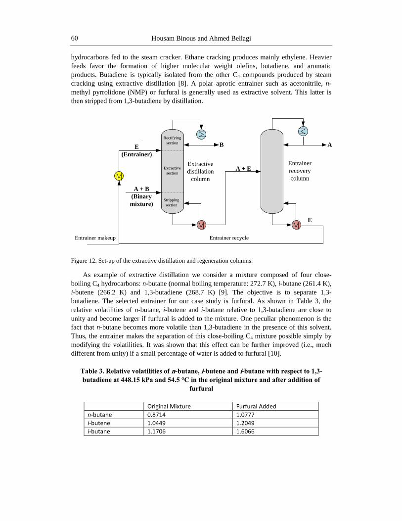
recovery (Figure 12).
In most industrialized countries, butadiene, an important monomer used in the production
of synthetic rubber, is produced as a byproduct of ethylene and other olefin production
processes by steam cracking [8]. If mixed with steam and subjected to pyrolysis, aliphatic
hydrocarbons give up hydrogen to yield mixtures of unsaturated hydrocarbons, including
butadiene. The quantity of butadiene produced depends on the nature of the aliphatic
Housam Binous and Ahmed Bellagi 60
hydrocarbons fed to the steam cracker. Ethane cracking produces mainly ethylene. Heavier
feeds favor the formation of higher molecular weight olefins, butadiene, and aromatic
products. Butadiene is typically isolated from the other C4 compounds produced by steam
cracking using extractive distillation [8]. A polar aprotic entrainer such as acetonitrile, n-
methyl pyrrolidone (NMP) or furfural is generally used as extractive solvent. This latter is
then stripped from 1,3-butadiene by distillation.
Figure 12. Set-up of the extractive distillation and regeneration columns.
As example of extractive distillation we consider a mixture composed of four close-
boiling C4 hydrocarbons: n-butane (normal boiling temperature: 272.7 K), i-butane (261.4 K),
i-butene (266.2 K) and 1,3-butadiene (268.7 K) [9]. The objective is to separate 1,3-
butadiene. The selected entrainer for our case study is furfural. As shown in Table 3, the
relative volatilities of n-butane, i-butene and i-butane relative to 1,3-butadiene are close to
unity and become larger if furfural is added to the mixture. One peculiar phenomenon is the
fact that n-butane becomes more volatile than 1,3-butadiene in the presence of this solvent.
Thus, the entrainer makes the separation of this close-boiling C4 mixture possible simply by
modifying the volatilities. It was shown that this effect can be further improved (i.e., much
different from unity) if a small percentage of water is added to furfural [10].
Table 3. Relative volatilities of n-butane, i-butene and i-butane with respect to 1,3-
butadiene at 448.15 kPa and 54.5 °C in the original mixture and after addition of
furfural
Original Mixture Furfural Added
n-butane 0.8714 1.0777
i-butene 1.0449 1.2049
i-butane 1.1706 1.6066
A + B
(Binary
mixture)
E
(Entrainer)
B
Entrainer recycleEntrainer makeup
Entrainer
recovery
column
Extractive
distillation
column
A + E
A
E
Extractive
section
Rectifying
section
Stripping
section
Simulation of the Separation of Industrially Important Hydrocarbon Mixtures ... 61
We now study several aspects related to this separation method by performing
simulations using Mathematica©, and Aspen HYSYS
® for comparison purposes. The Soave
Redlich-Kwong EoS (Appendix A) will be used and in both simulations. The solvent
regeneration column is also included in the simulations in order to show that the entrainer
recovery is possible.
Extractive Distillation Column
We consider an extractive distillation column with 50 equilibrium stages, a partial
reboiler and a total condenser and operating at 300 kPa. This column has an upper feed
composed of pure furfural (i.e., the entrainer) with a flow rate equal to 55 kmole/hr. It is
introduced at 20 °C at stage 3 counting from the top. The extractive column has also a lower
feed composed of 5 mol% n-butane, 15 mol% i-butene, 20 mol% i-butane and 60 mol% 1,3-
butadiene. The lower feed enters at stage 40 counting from the top at the same temperature of
20 °C with a flow rate of 10 kmole/hr. In the simulations, the mol% of 1,3-butadiene in the
distillate and of i-butene in the residue are set equal to 3 and 0.4, respectively.
The mathematical model of the separation sequence consists of MESH set of 678
nonlinear algebraic equations, which are solved in less than 33 seconds using Mathematica©.
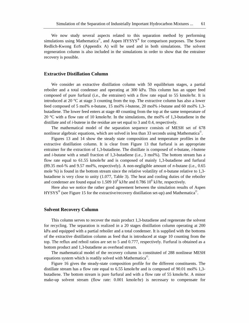
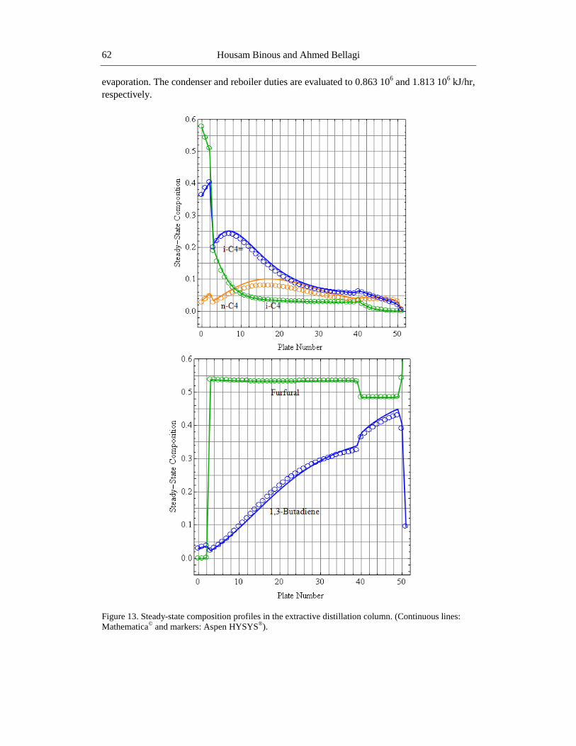
Figures 13 and 14 show the steady state composition and temperature profiles in the
extractive distillation column. It is clear from Figure 13 that furfural is an appropriate
entrainer for the extraction of 1,3-butadiene. The distillate is composed of n-butane, i-butene
and i-butane with a small fraction of 1,3-butadiene (i.e., 3 mol%). The bottom stream has a
flow rate equal to 61.55 kmole/hr and is composed of mainly 1,3-butadiene and furfural
(89.35 mol-% and 9.57 mol%, respectively). A non-negligible amount of n-butane (i.e., 0.65
mole %) is found in the bottom stream since the relative volatility of n-butane relative to 1,3-
butadiene is very close to unity (1.077, Table 3). The heat and cooling duties of the reboiler
and condenser are found equal to 1.509 106 kJ/hr and 0.786 10
6 kJ/hr, respectively.
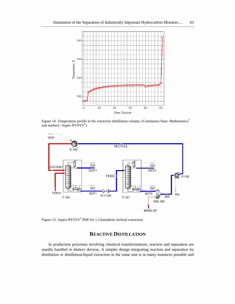
Here also we notice the rather good agreement between the simulation results of Aspen
HYSYS® (see Figure 15 for the extractive/recovery distillation set-up) and Mathematica
©.
Solvent Recovery Column
This column serves to recover the main product 1,3-butadiene and regenerate the solvent
for recycling. The separation is realized in a 20 stages distillation column operating at 200
kPa and equipped with a partial reboiler and a total condenser. It is supplied with the bottoms
of the extractive distillation column as feed that is introduced at stage 10 counting from the
top. The reflux and reboil ratios are set to 5 and 0.777, respectively. Furfural is obtained as a
bottom product and 1,3-butadiene as overhead stream.
The mathematical model of the recovery column is constituted of 288 nonlinear MESH
equations system which is readily solved with Mathematica©.
Figure 16 gives the steady-state composition profile for the different constituents. The
distillate stream has a flow rate equal to 6.55 kmole/hr and is composed of 90.01 mol% 1,3-
butadiene. The bottom stream is pure furfural and with a flow rate of 55 kmole/hr. A minor
make-up solvent stream (flow rate: 0.001 kmole/hr) is necessary to compensate for
Housam Binous and Ahmed Bellagi 62
evaporation. The condenser and reboiler duties are evaluated to 0.863 106 and 1.813 10
6 kJ/hr,
respectively.
Figure 13. Steady-state composition profiles in the extractive distillation column. (Continuous lines:
Mathematica© and markers: Aspen HYSYS
®).
Simulation of the Separation of Industrially Important Hydrocarbon Mixtures ... 63
Figure 14. Temperature profile in the extractive distillation column. (Continuous lines: Mathematica©
and markers: Aspen HYSYS®).
Figure 15. Aspen HYSYS® PDF for 1,3-butadiene furfural extraction.
REACTIVE DISTILLATION
In production processes involving chemical transformations, reaction and separation are
usually handled in distinct devices. A simpler design integrating reaction and separation by
distillation or distillation/liquid extraction in the same unit is in many instances possible and
Housam Binous and Ahmed Bellagi 64
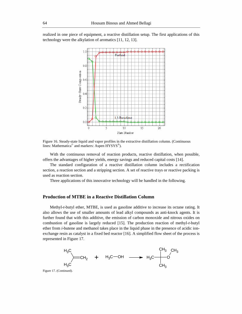
realized in one piece of equipment, a reactive distillation setup. The first applications of this
technology were the alkylation of aromatics [11, 12, 13].
Figure 16. Steady-state liquid and vapor profiles in the extractive distillation column. (Continuous
lines: Mathematica© and markers: Aspen HYSYS
®).
With the continuous removal of reaction products, reactive distillation, when possible,
offers the advantages of higher yields, energy savings and reduced capital costs [14].
The standard configuration of a reactive distillation column includes a rectification
section, a reaction section and a stripping section. A set of reactive trays or reactive packing is
used as reaction section.
Three applications of this innovative technology will be handled in the following.
Production of MTBE in a Reactive Distillation Column
Methyl-t-butyl ether, MTBE, is used as gasoline additive to increase its octane rating. It
also allows the use of smaller amounts of lead alkyl compounds as anti-knock agents. It is
further found that with this additive, the emission of carbon monoxide and nitrous oxides on
combustion of gasoline is largely reduced [15]. The production reaction of methyl-t-butyl
ether from i-butene and methanol takes place in the liquid phase in the presence of acidic ion-
exchange resin as catalyst in a fixed bed reactor [16]. A simplified flow sheet of the process is
represented in Figure 17.
Figure 17. (Continued).
CH2
CH3
CH3
+ CH3 OH
CH3
CH3
CH3 O
CH3
Simulation of the Separation of Industrially Important Hydrocarbon Mixtures ... 65
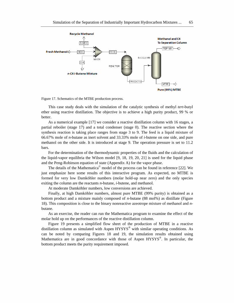
Figure 17. Schematics of the MTBE production process.
This case study deals with the simulation of the catalytic synthesis of methyl tert-butyl
ether using reactive distillation. The objective is to achieve a high purity product, 99 % or
better.
As a numerical example [17] we consider a reactive distillation column with 16 stages, a
partial reboiler (stage 17) and a total condenser (stage 0). The reactive section where the
synthesis reaction is taking place ranges from stage 3 to 9. The feed is a liquid mixture of
66.67% mole of n-butane as inert solvent and 33.33% mole of i-butene on one side, and pure
methanol on the other side. It is introduced at stage 9. The operation pressure is set to 11.2
bars.
For the determination of the thermodynamic properties of the fluids and the calculation of
the liquid-vapor equilibria the Wilson model [9, 18, 19, 20, 21] is used for the liquid phase
and the Peng-Robinson equation of state (Appendix A) for the vapor phase.
The details of the Mathematica© model of the process can be found in reference [22]. We
just emphasize here some results of this interactive program. As expected, no MTBE is
formed for very low Damköhler numbers (molar hold-up near zero) and the only species
exiting the column are the reactants n-butane, i-butene, and methanol.
At moderate Damköhler numbers, low conversions are achieved.
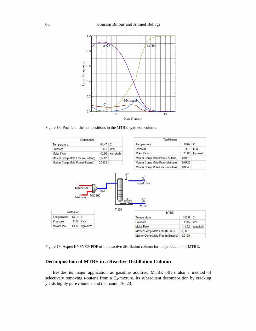
Finally, at high Damköhler numbers, almost pure MTBE (99% purity) is obtained as a
bottom product and a mixture mainly composed of n-butane (88 mol%) as distillate (Figure
18). This composition is close to the binary nonreactive azeotrope mixture of methanol and n-
butane.
As an exercise, the reader can run the Mathematica program to examine the effect of the
molar hold up on the performances of the reactive distillation column.
Figure 19 presents a simplified flow sheet of the production of MTBE in a reactive
distillation column as simulated with Aspen HYSYS® with similar operating conditions. As
can be noted by comparing Figures 18 and 19, the simulation results obtained using
Mathematica are in good concordance with those of Aspen HYSYS®. In particular, the
bottom product meets the purity requirement imposed.
Housam Binous and Ahmed Bellagi 66
Figure 18. Profile of the compositions in the MTBE synthesis column.
Figure 19. Aspen HYSYS® PDF of the reactive distillation column for the production of MTBE.
Decomposition of MTBE in a Reactive Distillation Column
Besides its major application as gasoline additive, MTBE offers also a method of
selectively removing i-butene from a C4-mixture. Its subsequent decomposition by cracking
yields highly pure i-butene and methanol [16, 23].
Simulation of the Separation of Industrially Important Hydrocarbon Mixtures ... 67
In the present case study we simulate a reactive distillation column that produces i-butene
and methanol from the decomposition of methyl tert-butyl ether (MTBE), the reverse reaction
of that of the preceding case.
The reaction is taking place in the liquid phase in the presence of acid catalyst. Distilling
the decomposition products under reflux yields an overhead fraction composed mainly of i-
butene and bottoms effluent containing almost pure methanol.
The sieve tray column has 16 stages, a partial reboiler, and a total condenser. The column
is fed with pure MTBE at stage 8. The reactive stages range from 6 to 11.
An asymmetric thermodynamic approach (−) is used to predict the properties of the
fluid mixture and the calculation of the liquid-vapor equilibria: Wilson model for the liquid
phase and ideal gas law for the vapor phase. The operation pressure is set to 11.2 bars. The
details of the kinetics of this equilibrium limited reaction can be found in references [24, 25].
The Mathematica© interactive simulation model of this reactive distillation column can be
found in reference [25]. Figures 20 and 21 are generated with this program. The reader is
encouraged to run the program in order to study the effect of the operating conditions on the
purity of the distillate.
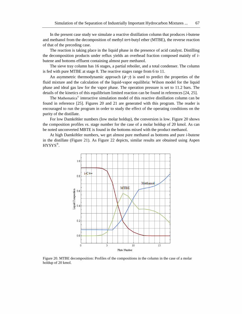
For low Damköhler numbers (low molar holdup), the conversion is low. Figure 20 shows
the composition profiles vs. stage number for the case of a molar holdup of 20 kmol. As can
be noted unconverted MBTE is found in the bottoms mixed with the product methanol.
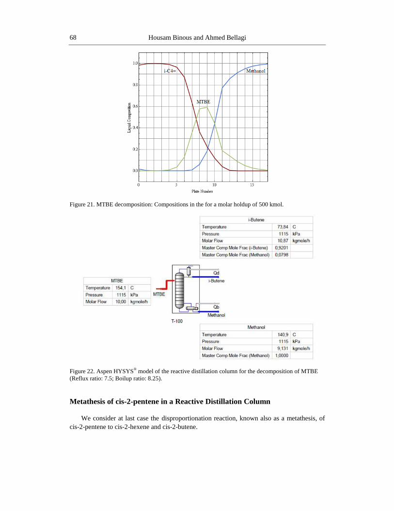
At high Damköhler numbers, we get almost pure methanol as bottoms and pure i-butene
in the distillate (Figure 21). As Figure 22 depicts, similar results are obtained using Aspen
HYSYS®.
Figure 20. MTBE decomposition: Profiles of the compositions in the column in the case of a molar
holdup of 20 kmol.
Housam Binous and Ahmed Bellagi 68
Figure 21. MTBE decomposition: Compositions in the for a molar holdup of 500 kmol.
Figure 22. Aspen HYSYS® model of the reactive distillation column for the decomposition of MTBE
(Reflux ratio: 7.5; Boilup ratio: 8.25).
Metathesis of cis-2-pentene in a Reactive Distillation Column
We consider at last case the disproportionation reaction, known also as a metathesis, of
cis-2-pentene to cis-2-hexene and cis-2-butene.
Simulation of the Separation of Industrially Important Hydrocarbon Mixtures ... 69
In order to simplicity the notations, we designate by C, B and A respectively the
components cis-2-pentene, cis-2-hexene and cis-2-butene.
The ternary mixture is subject to an equilibrium-limited chemical reaction with reaction
rate [26, 27]
where Keq is the temperature dependant equilibrium constant, and
the reaction rate constant, with R = 1.987 cal mol-1
K-1
.
The pure reactant C (cis-2-pentene) is fed to a reactive distillation column operating at a
pressure of 3 atmospheres with 13 plates; the feed stage location is stage 5, the reactive stages
go from stages 2 to 7. The feed flow rate is set to 100kmol/hr.
The following simulations are made with the simplifying assumption of constant molar
overflow (CMO) and by neglecting heat effects [6, 27, 28].
The Mathematica© interactive simulation model of this reactive distillation column can
be found in reference [28]. Figures 23, 24 and 25 illustrate some results of the calculations,
namely:
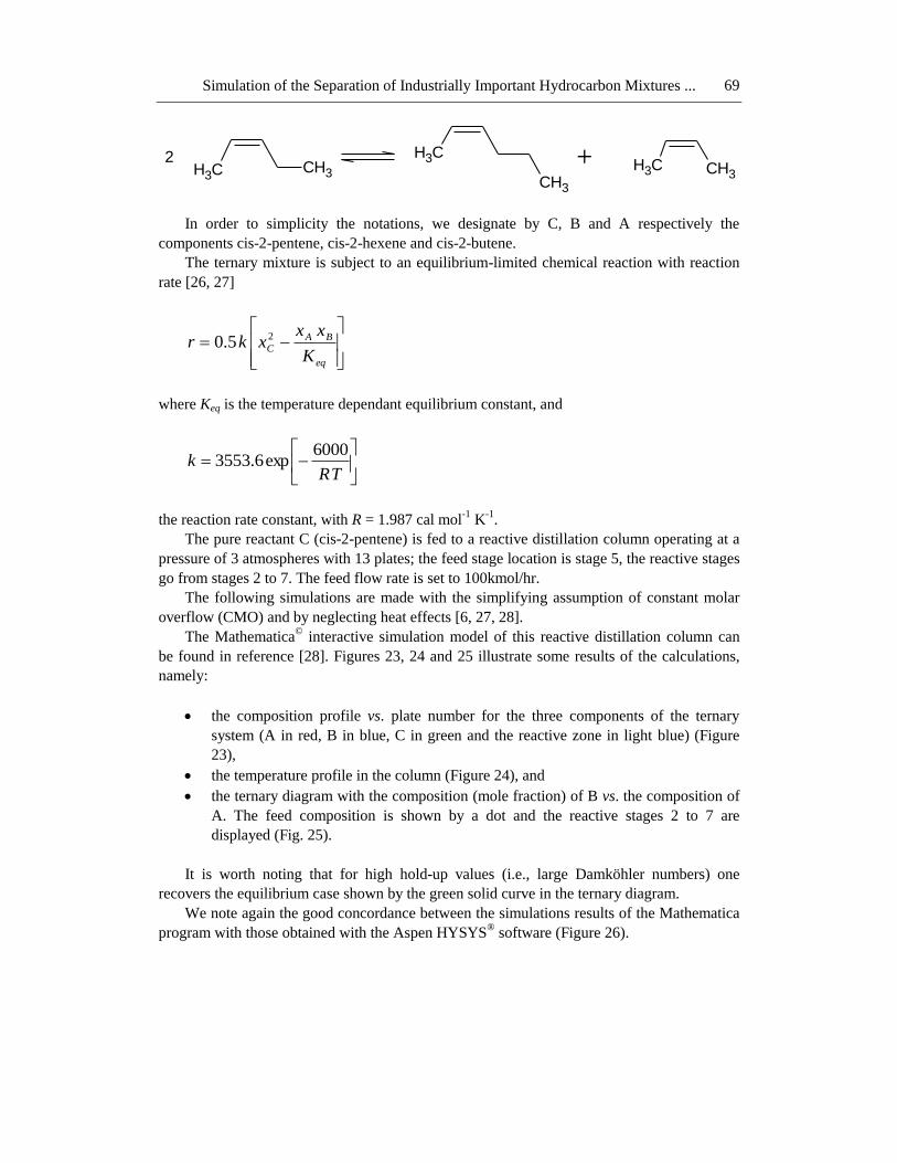
the composition profile vs. plate number for the three components of the ternary
system (A in red, B in blue, C in green and the reactive zone in light blue) (Figure
23),
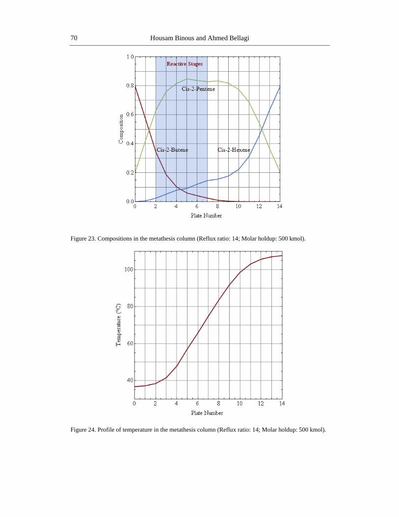
the temperature profile in the column (Figure 24), and
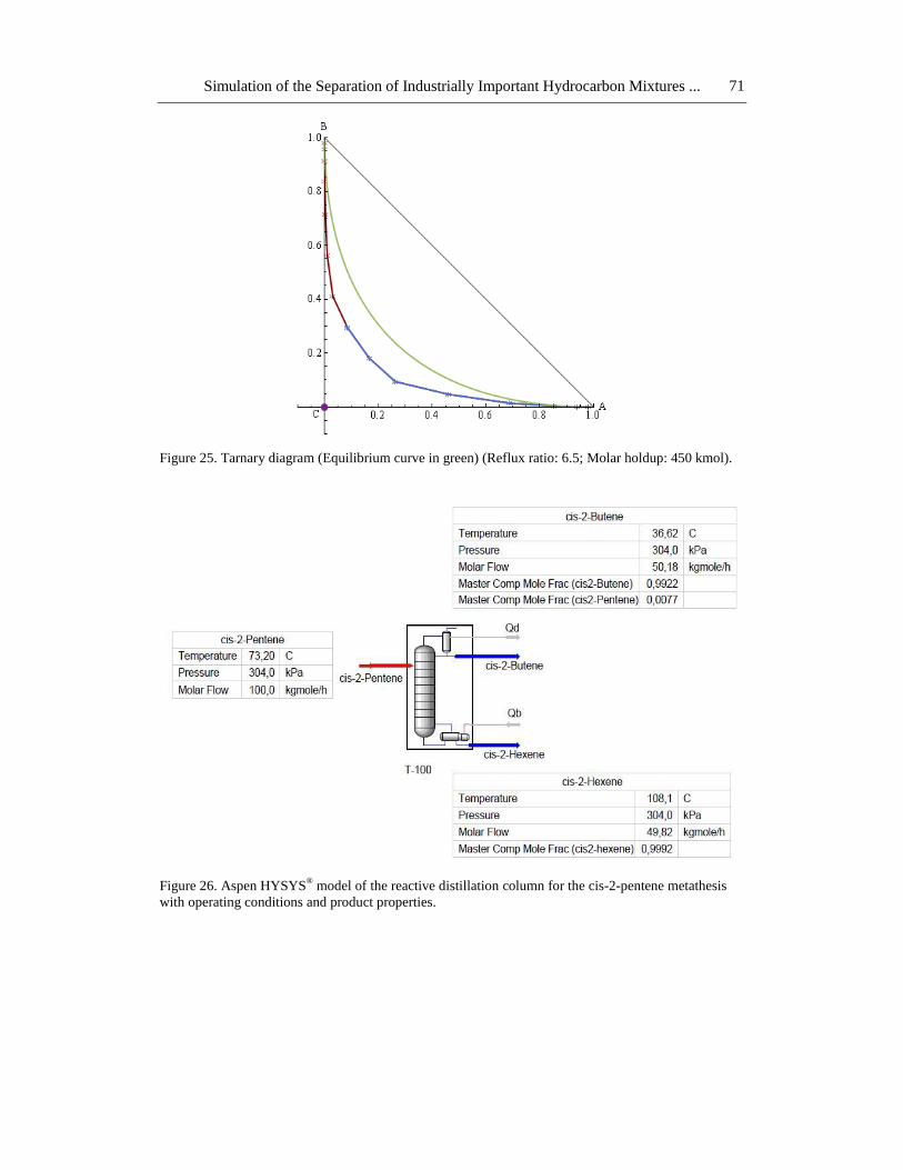
the ternary diagram with the composition (mole fraction) of B vs. the composition of
A. The feed composition is shown by a dot and the reactive stages 2 to 7 are
displayed (Fig. 25).
It is worth noting that for high hold-up values (i.e., large Damköhler numbers) one
recovers the equilibrium case shown by the green solid curve in the ternary diagram.
We note again the good concordance between the simulations results of the Mathematica
program with those obtained with the Aspen HYSYS® software (Figure 26).
CH3CH3
CH3
CH3
+ CH3 CH3
2
eq
BAC
K
xxxkr 25.0
TRk
6000exp6.3553
Housam Binous and Ahmed Bellagi 70
Figure 23. Compositions in the metathesis column (Reflux ratio: 14; Molar holdup: 500 kmol).
Figure 24. Profile of temperature in the metathesis column (Reflux ratio: 14; Molar holdup: 500 kmol).
Simulation of the Separation of Industrially Important Hydrocarbon Mixtures ... 71
Figure 25. Tarnary diagram (Equilibrium curve in green) (Reflux ratio: 6.5; Molar holdup: 450 kmol).
Figure 26. Aspen HYSYS® model of the reactive distillation column for the cis-2-pentene metathesis
with operating conditions and product properties.
Housam Binous and Ahmed Bellagi 72
EXPLORING FURTHER PEDAGOGICAL PROBLEMS
USING MATHEMATICA©
In all the distillation simulations presented for the different case studies, no optimizations
have been attempted. Indeed, the number of trays, the feed tray locations as well as the reflux
and reboil ratios could be varied easily in order to come-up with more economical designs.
For this purpose, TAC calculations [29] could be performed. In addition, column diameters
could be determined based on the classical procedure by Fair [30, 31]. In principle, it would
also be possible with the help of Mathematica© to perform even dynamic simulations for
these distillation columns [32] and then to device appropriate control schemes [33].
For the case of extractive distillation, solvents other than furfural could be used. For
example, NMP is known to be a very good candidate for the purification of C4 mixtures
containing 1,3-butadiene. Such calculations would require: (1) a good activity coefficient
prediction model such as the UNIQUAC model [9, 19, 20, 34] to allow for non-ideal behavior
in the liquid phase and (2) an EoS such as the SRK or PR EoS to predict the gas-phase
fugacity coefficients since the column operates at relatively high pressures.
CONCLUSION
In this chapter five industrially relevant fractionation processes by different distillation
techniques are simulated: the separation of natural gas liquids (NGLs) in a distillation train,
the extractive distillation of 1,3-butadiene from a C4 cut with furfural as the entrainer, the
production of MTBE from i-butene and methanol in a reactive distillation column, the reverse
process of production of i-butene by the decomposition of methyl tert-butyl ether, and the
metathesis of cis-2-pentene to cis-2-butene and cis-2-hexene.
Routinely these processes are treated readily using a flow sheeting software like Aspen-
HYSYS®, similarly to what is done here for comparison purposes. The objective of this
chapter was to show how these complex processes can also be handled with more pedagogical
benefits using the computer algebra Mathematica®. In all investigated cases, the comparison
between the two approaches of simulations shows very good agreement.
The Mathematica© interactive simulation models developed for the different case studies
are available at http://demonstrations.wolfram.com.
REFERENCES
[1] Devold H. Oil and Gas Production Handbook, Edition 2.3, Oslo: ABB, 2010.
[2] Kidnay, A. J. & Parrish, W. R. Fundamentals of Natural Gas Processing, Boca Raton:
Taylor and Francis, 2006.
[3] Maddox R. N. & Erbar J. H. Gas Conditioning and Processing, Campbell Petroleum
Series, Volume 3, Oklahoma: 1992.
[4] Younger, A. H. & Eng., P. Natural Gas Processing Principles and Technology, Part II,
University of Calgary, 2004.
Simulation of the Separation of Industrially Important Hydrocarbon Mixtures ... 73
[5] Wankat, P. C. Separation Process Engineering, 2nd
Edition, Upper Saddle River:
Prentice Hall, 2007.
[6] Doherty, M. F. & Malone, M. F. Conceptual Design of Distillation Systems, New York:
McGraw–Hill, 2001.
[7] Lei, Z., Li, C. & Chen, B. “Extractive Distillation: a Review,” Separation and
Purification Reviews, 32, pp. 121-213, 2003.
[8] Sun, H. P. & Wristers, J. P. Butadiene, Encyclopedia of Chemical Technology, Volume
4, 4th Edition, New York: John Wiley & Sons, 1992.
[9] Reid, C. R., Prausnitz, J. M. & Poling, B. E. The properties of Gases and Liquids, 4th
Edition, McGraw-Hill, Inc., 1987.
[10] Buell C. K., & Boatright R. G. “Furfural Extractive Distillation,” Industrial and
Engineering Chemistry, 39, pp. 695–705, 1947.
[11] Smith, L. A. US Patent 4 849 569, 1989; US Patent, 5 446 223, 1995.
[12] Hsieh et al. US Patent 5 082990, 1992.
[13] Dimian, A. C. & Bildea, C. S. Chemical Process Design, Weinheim: Wiley-VCH
Verlag GmbH & Co., 2008.
[14] Process Modeling Using HYSYS With Chemical Industry Focus, ASPEN HYSYS
Documentation, 2004.
[15] Adams, J. M., Clement, D. E. & Graham, S. H. Clays and Clay Minerals, Vol. 30, No.
2, pp. 129-134, 1982.
[16] Speight, J.G Chemical and Process Design Handbook, McGraw-Hill, Inc., 2002.
[17] Chen, F., Huss, R. S., Malone, M. F. & Doherty, M. F. "Simulation of Kinetic Effects
in Reactive Distillation" Computers and Chemical Engineering, 24(11), pp. 2457–2472,
2000.
[18] Wilson, G. M. “Vapor-Liquid Equilibrium XI: a new expression for the excess free
energy of mixing”, Journal of the American Chemical Society, Vol. 86, pp. 127-130,
1964.
[19] Sandler, S. I. Chemical Engineering Thermodynamics, 3rd
Edition, John Wiley and
Sons, 1999.
[20] Poling, B. E., Prausnitz, J. M. & O’Connell, J. P. The properties of Gases and Liquids,
5th Edition, McGraw-Hill, Inc., 2001.
[21] Binous, H. Computation of Residue Curves Using Mathematica and Matlab, in
Computer Simulations, Boris Nemanjic and Navenka Svetozar Editors, Nova Science
Publishers, Inc., pp. 161-173, 2013.
[22] Binous, H., Selmi, M., Wada, I., Allouche, S. & Bellagi, A. “Methyl Tert-Butyl Ether
(MTBE) Synthesis with a Reactive Distillation Unit”, Wolfram Demonstrations Project:
http://demonstrations.wolfram.com/MethylTertButylEtherMTBESynthesisWithAReacti
veDistillationUn/
[23] Deguchi T. & Tokumaru T. Patent EP 0068785A1, 1983.
[24] Huang K. & Wang S. J. “Design and Control of a Methyl Tertiary Butyl Ether (MTBE)
Decomposition Reactive Distillation Column”, Ind. Eng. Chem. Res., 46(8), pp. 2508–
2519, 2007.
[25] Binous H., Selmi M., Wada I. Allouche S. & Bellagi A. “Methyl Tert-Butyl Ether
(MTBE) Decomposition with a Reactive Distillation Unit”, Wolfram Demonstrations
Project:
Housam Binous and Ahmed Bellagi 74
http://demonstrations.wolfram.com/MethylTertButylEtherMTBEDecompositionWithA
ReactiveDistillation/
[26] Dragomir, R. M. & Jobson, M. “Conceptual Design of Single-Feed Kinetically
Controlled Reactive Distillation Columns”, Chemical Engineering Science, 60(18), pp.
5049–5068, 2005.
[27] Doherty, M. F. & Knapp, J. P. “Distillation, Azeotropic and Extractive,” in Kirk-
Othmer Encyclopedia of Chemical Technology, New York: John Wiley & Sons, 2004.
[28] Binous, H., Selmi, M., Wada, I. Allouche, S. & Bellagi, A. “Production of Cis2-Butene
and Cis2-Hexene by Cis2-Pentene Disproportionation”, Wolfram Demonstrations
Project, http://demonstrations.wolfram.com/ProductionOfCis2ButeneAndCis2 Hexene
ByCis2PenteneDisproportion/
[29] Douglas, J. M. Conceptual Design of Chemical Processes, International Edition, New
York: McGraw–Hill, 1988.
[30] Perry, R. H. & Green, D. W. Editors. Perry’s Chemical Engineers’ Handbook,
International Edition, 7th
Edition, New York: McGraw–Hill, pp. 14-27, 1997.
[31] Seader, J. D. & Henley, R. H. Separation Process Principles, New York: John Wiley
and Sons, Inc., 1998.
[32] Nasri, Z. & Binous, H. “Rigorous Distillation Dynamics Simulations Using a Computer
Algebra”, Computer Applications in Engineering Education, 20, pp. 193–202, 2012.
[33] Luyben, W. L. Distillation Design and Control Using Aspen Simulation, New York:
Wiley, 2006.
[34] Tester, J. W. & Modell, M. Thermodynamics and its Applications, 3rd
Edition, Prentice
Hall International, 1997.
[35] Peng, D. Y. & Robinson D. B. "A New Two-Constant Equation of State", Industrial
and Engineering Chemistry: Fundamentals, 15, pp. 59-64, 1976.
[36] Soave, G. "Equilibrium Constants from a Modified Redlich-Kwong Equation of State",
Chemical Engineering Science, 27, pp. 1197–1203, 1972.
[37] Nasri, Z. & Binous H. “Applications of the Soave-Redlich-Kwong Equation of State
Using Mathematica®”, Journal of Chemical Engineering of Japan, 40, pp. 534-538,
2007.
[38] Nasri, Z. & Binous H. “Applications of the Peng-Robinson Equation of State using
MATLAB”, Chemical Engineering Education, 43, pp. 115-124 (2009).
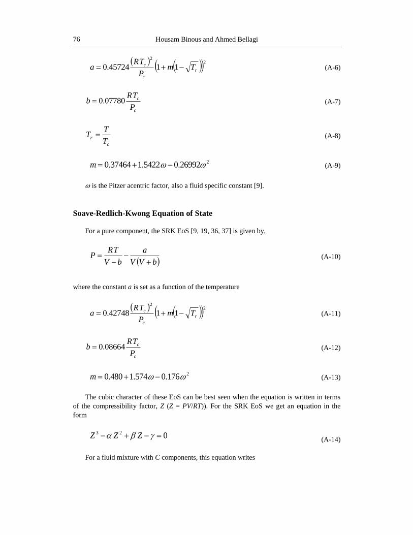
APPENDIX A:
CUBIC EQUATIONS OF STATE
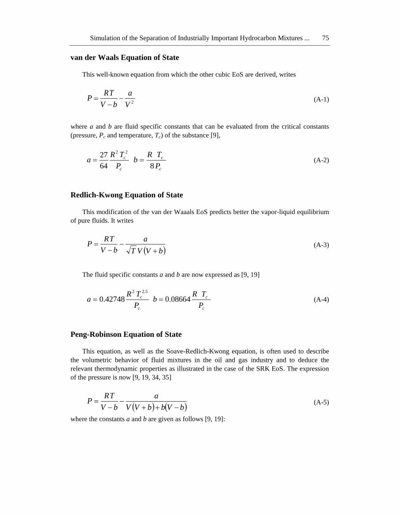
Cubic equation of states are pressure explicit equation in temperature and volume that,
when expanded, would contain the volume raised to the third power. They are often used in
the oil and gas and petrochemical industries to describe the behavior of the fluid mixtures.
They allow the prediction of several important aspects of chemical engineering
thermodynamics such as vapor-liquid equilibrium data, liquid-phase and vapor-phase
compressibility factors, enthalpies of gases and liquids, etc. Simulations of the distillation of
several industrially relevant hydrocarbon mixtures commonly build on equations of states
such as the SRK and PR EoS.
Simulation of the Separation of Industrially Important Hydrocarbon Mixtures ... 75
van der Waals Equation of State
This well-known equation from which the other cubic EoS are derived, writes
(A-1)
where a and b are fluid specific constants that can be evaluated from the critical constants
(pressure, Pc and temperature, Tc) of the substance [9],
(A-2)
Redlich-Kwong Equation of State
This modification of the van der Waaals EoS predicts better the vapor-liquid equilibrium
of pure fluids. It writes
(A-3)
The fluid specific constants a and b are now expressed as [9, 19]
(A-4)
Peng-Robinson Equation of State
This equation, as well as the Soave-Redlich-Kwong equation, is often used to describe
the volumetric behavior of fluid mixtures in the oil and gas industry and to deduce the
relevant thermodynamic properties as illustrated in the case of the SRK EoS. The expression
of the pressure is now [9, 19, 34, 35]
(A-5)
where the constants a and b are given as follows [9, 19]:
2V
a
bV
TRP
c
c
P
TRa
22
64
27
c
c
P
TRb
8
bVVT
a
bV
TRP
c
c
P
TRa
5.22
42748.0c
c
P
TRb 08664.0
bVbbVV
a
bV
TRP
Housam Binous and Ahmed Bellagi 76
(A-6)
(A-7)
(A-8)
(A-9)
is the Pitzer acentric factor, also a fluid specific constant [9].
Soave-Redlich-Kwong Equation of State
For a pure component, the SRK EoS [9, 19, 36, 37] is given by,
(A-10)
where the constant a is set as a function of the temperature
(A-11)
(A-12)
(A-13)
The cubic character of these EoS can be best seen when the equation is written in terms
of the compressibility factor, Z (Z = PV/RT)). For the SRK EoS we get an equation in the
form
(A-14)
For a fluid mixture with C components, this equation writes
22
1145724.0 r
c
c TmP
TRa
c
c
P
TRb 07780.0
c
rT
TT
226992.05422.137464.0 m
bVV
a
bV
TRP
22
1142748.0 r
c
c TmP
TRa
c
c
P
TRb 08664.0
2176.0574.1480.0 m
023 ZZZ
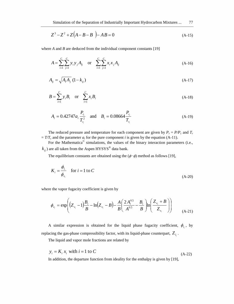
Simulation of the Separation of Industrially Important Hydrocarbon Mixtures ... 77
(A-15)
where A and B are deduced from the individual component constants [19]
(A-16)
(A-17)
(A-18)
(A-19)
The reduced pressure and temperature for each component are given by Pr = P/Pc and Tr
= T/Tc and the parameter ai for the pure component i is given by the equation (A-11).
For the Mathematica©
simulations, the values of the binary interaction parameters (i.e.,
) are all taken from the Aspen HYSYS® data bank.
The equilibrium constants are obtained using the (−) method as follows [19],
(A-20)
where the vapor fugacity coefficient is given by
(A-21)
A similar expression is obtained for the liquid phase fugacity coefficient, , by
replacing the gas-phase compressibility factor, with its liquid-phase counterpart, .
The liquid and vapor mole fractions are related by
(A-22)
In addition, the departure function from ideality for the enthalpy is given by [19],
023 BABBAZZZ
C
i
C
j
ijji
C
i
C
j
ijji AxxAyyA1 11 1
or
)1( ijjiij kAAA
C
i
ii
C
i
ii BxByB11
or
i
i
i
i
r
r
i
r
r
iiT
PB
T
PaA 08664.0and42747.0
2
ijk
CiK
i
i
v
l
i to1for
i
i
iii
v
vii
v
i
vvZ
BZ
B
B
A
A
B
ABZ
B
BZ ln
2ln1exp
5.0
5.0
il
ilZ
CixKy iii to1with
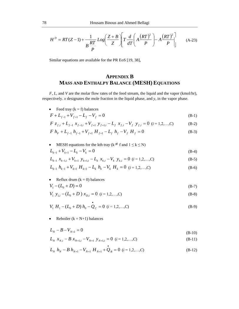
Housam Binous and Ahmed Bellagi 78
(A-23)
Similar equations are available for the PR EoS [19, 38],
APPENDIX B
MASS AND ENTHALPY BALANCE (MESH) EQUATIONS
F, L, and V are the molar flow rates of the feed stream, the liquid and the vapor (kmol/hr),
respectively. x designates the mole fraction in the liquid phase, and y, in the vapor phase.
Feed tray (k = f) balances
(B-1)
(i = 1,2,…,C) (B-2)
(B-3)
MESH equations for the kth tray (k f and 1 ≤ k ≤ N)
(B-4)
(i = 1,2,…,C) (B-5)
(i = 1,2,…,C) (B-6)
Reflux drum (k = 0) balances
(B-7)
(i = 1,2,…,C) (B-8)
(i = 1,2,…,C) (B-9)
Reboiler (k = N+1) balances
(B-10)
(i = 1,2,…,C) (B-11)
(i = 1,2,…,C) (B-12)
P
RTA
P
RTA
dT
dT
Z
BZLog
P
RTB
ZRTH D
221
)1(
011 ffff VLVLF
0,,,11,11, iffiffiffiffif yVxLyVxLzF
01111 ffffffffF HVhLHVhLhF
011 kkkk VLVL
0,,,11,11 ikkikkikkikk yVxLyVxL
01111 kkkkkkkk HVhLHVhL
0)( 01 DLV
0)( ,0,11 iDi xDLyV
0)( 0011
CQhDLHV
01 NN VBL
0,11,1, iNNiNiNN yVxBxL
0111
BNNNNN QHVhBhL