Embed Size (px)
Citation preview
HOUGH TRANSFORM
Presentation by Sumit TandonDepartment of Electrical Engineering University of Texas at Arlington
Course # EE6358 Computer Vision

EE6358 - Computer Vision 2
Contents Introduction Advantages of Hough transform Hough Transform for Straight Line
Detection Hough Transform for Circle Detection Recap and list of parameters Generalized Hough Transform Improvisation of Hough Transform Examples References

EE6358 - Computer Vision 3
1. Introduction Performed after Edge Detection It is a technique to isolate the curves of a
given shape / shapes in a given image Classical Hough Transform can locate
regular curves like straight lines, circles, parabolas, ellipses, etc. Requires that the curve be specified in some
parametric form Generalized Hough Transform can be used
where a simple analytic description of feature is not possible

EE6358 - Computer Vision 4
2. Advantages of Hough Transform
The Hough Transform is tolerant of gaps in the edges
It is relatively unaffected by noise It is also unaffected by occlusion in
the image

EE6358 - Computer Vision 5
3.1 Hough Transform for Straight Line Detection A straight line can be represented as
y = mx + c This representation fails in case of vertical lines
A more useful representation in this case is
Demo

EE6358 - Computer Vision 6
3.2 Hough Transform for Straight Lines
Advantages of Parameterization Values of ‘’ and ‘’ become bounded
How to find intersection of the parametric curves Use of accumulator arrays – concept of
‘Voting’ To reduce the computational load use
Gradient information

EE6358 - Computer Vision 7
3.3 Computational Load
Image size = 512 X 512 Maximum value of With a resolution of 1o, maximum
value of Accumulator size = Use of direction of gradient reduces
the computational load by 1/360
22*512
360360*22*512

EE6358 - Computer Vision 8
3.4 Hough Transform for Straight Lines - Algorithm Quantize the Hough Transform space: identify the
maximum and minimum values of and Generate an accumulator array A(, ); set all values
to zero For all edge points (xi, yi) in the image
Use gradient direction for Compute from the equation Increment A(, ) by one
For all cells in A(, ) Search for the maximum value of A(, ) Calculate the equation of the line
To reduce the effect of noise more than one element (elements in a neighborhood) in the accumulator array are increased

EE6358 - Computer Vision 9
3.5 Line Detection by Hough Transform

EE6358 - Computer Vision 10
4.1 Hough Transform for Detection of Circles
The parametric equation of the circle can be written as
The equation has three parameters – a, b, r The curve obtained in the Hough Transform
space for each edge point will be a right circular cone
Point of intersection of the cones gives the parameters a, b, r
222 )()( rbyax
EE6358 - Computer Vision 11
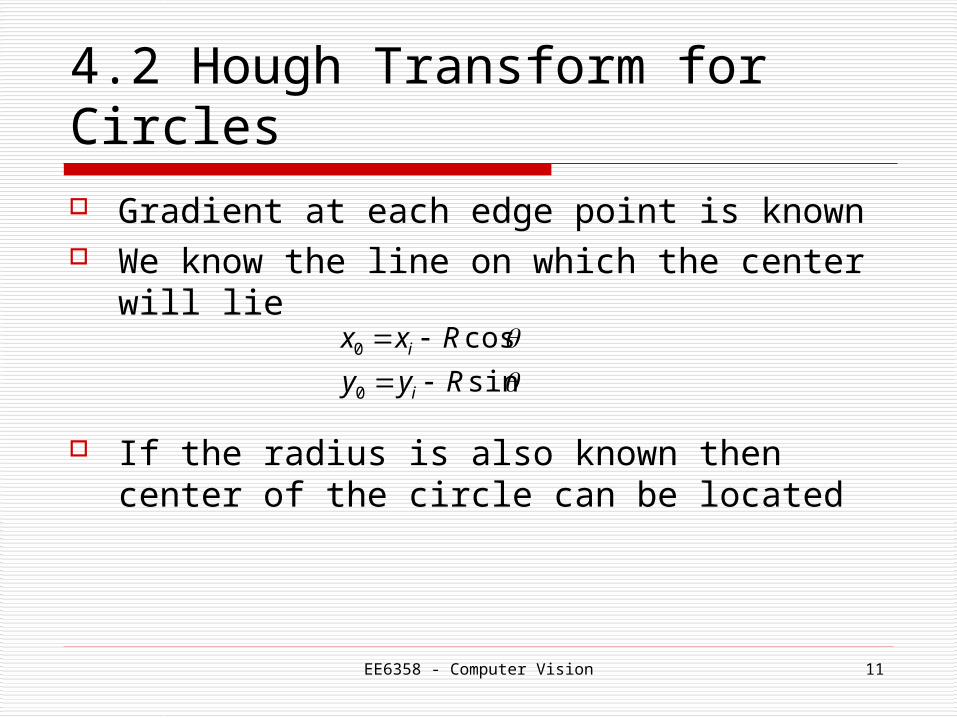
4.2 Hough Transform for Circles Gradient at each edge point is known We know the line on which the center will
lie
If the radius is also known then center of the circle can be located
sin
cos
0
0
Ryy
Rxx
i
i

EE6358 - Computer Vision 12
4.3 Detection of circle by Hough Transform - example
Original Image Circles detected by Canny Edge Detector

EE6358 - Computer Vision 13
4.4 Detection of circle by Hough Transform - contd
Hough Transform of the edge detected image Detected Circles

EE6358 - Computer Vision 14
5.1 Recap In detecting lines
The parameters and were found out relative to the origin (0,0)
In detecting circles The radius and center were found out
In both the cases we have knowledge of the shape
We aim to find out its location and orientation in the image
The idea can be extended to shapes like ellipses, parabolas, etc.

EE6358 - Computer Vision 15
5.2 Parameters for analytic curves
Analytic Form Parameters Equation
Line , xcos+ysin=
Circle x0, y0, (x-xo)2+(y-y0)2=r2
Parabola x0, y0, (y-y0)2=4(x-xo)
Ellipse x0, y0, a, b, (x-xo)2/a2+(y-y0)2/b2=1
EE6358 - Computer Vision 16
6.1 Generalized Hough Transform
The Generalized Hough transform can be used to detect arbitrary shapes
Complete specification of the exact shape of the target object is required in the form of the R-Table
Information that can be extracted are Location Size Orientation Number of occurrences of that particular shape

EE6358 - Computer Vision 17
6.2 Creating the R-table
Algorithm Choose a reference point Draw a vector from the reference point
to an edge point on the boundary Store the information of the vector
against the gradient angle in the R-Table There may be more than one entry in the
R-Table corresponding to a gradient value

EE6358 - Computer Vision 18
6.3 Generalized Hough Transform - Algorithm Form an Accumulator array to hold the candidate
locations of the reference point For each point on the edge
Compute the gradient direction and determine the row of the R-Table it corresponds to
For each entry on the row calculate the candidate location of the reference point
Increase the Accumulator value for that point The reference point location is given by the highest
value in the accumulator array
sin
cos
ryy
rxx
ic
ic

EE6358 - Computer Vision 19
6.4 Generalized Hough Transform – Size and Orientation
The size and orientation of the shape can be found out by simply manipulating the R-Table
For scaling by factor S multiply the R-Table vectors by S
For rotation by angle , rotate the vectors in the R-Table by angle

EE6358 - Computer Vision 20
6.5 Generalized Hough Transform – Advantages and disadvantages
Advantages A method for object recognition Robust to partial deformation in shape Tolerant to noise Can detect multiple occurrences of a
shape in the same pass Disadvantages
Lot of memory and computation is required

EE6358 - Computer Vision 21
7.1 Improvisation of the Hough transform for detecting straight line segments
Hough Transform lacks the ability to detect the end points of lines – localized information is lost during HT
Peak points in the accumulator can be difficult to locate in presence of noisy or parallel edges
Efficiency of the algorithm decreases if image becomes too large
New approach is proposed to reduce these problems

EE6358 - Computer Vision 22
7.2 Spatial decomposition This technique preserves the localized
information Divide the image recursively into
quad-trees, each quad-tree representing a part of the image i.e. a sub-image
The leaf nodes will be voted for feature points which are in the sub-image represented by the leaf node

EE6358 - Computer Vision 23
7.2 Spatial Decomposition of Hough Transform Parameter space is defined from a global
origin rather than a local one Each node contains information about the
sub-nodes as well as the number of feature points in the sub-image represented by the node
Pruning of sub-trees is done if the number of the feature points falls below a threshold
An accumulator is assigned for each leaf node

EE6358 - Computer Vision 24
7.3 Some relations involved in spatial decomposition Consider the following
Q – any non-leaf node F – feature points in the sub-image represented by
this node A – parameter space of the sub-image
The following relations hold true

EE6358 - Computer Vision 25
7.4 Number of accumulator arrays required
Consider the following case Size of image = N X N Size of leaf node = M X M Depth of tree = d (root node = 0)
Number of accumulator arrays for only leaf nodes =
Number of accumulator arrays for all nodes =

EE6358 - Computer Vision 26
7.5 Example

EE6358 - Computer Vision 27
References Generalizing The Hough Transform to Detect Arbitrary
Shapes – D H Ballard – 1981 Spatial Decomposition of The Hough Transform –
Heather and Yang – IEEE computer Society – May 2005
Hypermedia Image Processing Reference 2 – http://homepages.inf.ed.ac.uk/rbf/HIPR2/hipr_top.htm
Machine Vision – Ramesh Jain, Rangachar Kasturi, Brian G Schunck, McGraw-Hill, 1995
Machine Vision - Wesley E. Snyder, Hairong Qi, Cambridge University Press, 2004