Hotspot identification for Mapper graphs

Ciara F. Loughrey1, Nick Orr2, Anna Jurek-Loughrey1

1School of Electronics, Electrical Engineering and Computer Science2Patrick G Johnston Centre for Cancer Research

Queen’s University Belfast, Northern Ireland{cloughrey11, nick.orr, a.jurek} @qub.ac.uk

Paweł DłotkoDioscuri Centre in Topological Data Analysis

Mathematical Institute, Polish Academy of Sciences Warsaw, Polandpdlotko@impan.pl

Abstract

Mapper algorithm can be used to build graph-based representations of high-dimensional data capturing structurally interesting features such as loops, flares orclusters. The graph can be further annotated with additional colouring of verticesallowing location of regions of special interest. For instance, in many applications,such as precision medicine, Mapper graph has been used to identify unknowncompactly localized subareas within the dataset demonstrating unique or unusualbehaviours. This task, performed so far by a researcher, can be automatized usinghotspot analysis. In this work we propose a new algorithm for detecting hotspotsin Mapper graphs. It allows automatizing of the hotspot detection process. Wedemonstrate the performance of the algorithm on a number of artificial and realworld datasets. We further demonstrate how our algorithm can be used for theautomatic selection of the Mapper lens functions.

1 Introduction

The aim of hotspot analysis is to detect anomalous regions, such as subgroups of patients with distinc-tive survival, within a dataset. Those regions could indicate a novel phenomena (e.g. the existence ofan unknown disease type (Nicolau et al. (2011); Lum et al. (2013); Cho et al. (2019)). The Mapperalgorithm (summarized in S1.1) generates a graph representation of the layout of multidimensionaldata samples. The original data points are mapped to the low-dimensional space according to the lensfunction of the algorithm, also known as the filter function. Once an appropriate lens function is used,the hotspots in the data and hotspots in the Mapper graph will be in correspondence. ConsequentlyMapper graphs provide a handy way to detect hotspots. There are however two issues; Firstly, manualanalysis of large graphs, that are often obtained for large datasets, is prohibitive. Secondly, selectionof appropriate parameters for Mapper construction that reveal the hotspots in data is nontrivial andtypically requires the construction of multiple Mapper graphs that need to be analyzed. In order toaddress this challenge we propose a new technique for automatic detection of hotspots in graphs.Using a real-world breast cancer dataset, we demonstrate how the proposed algorithm can be usedto automatically select a lens function based on its ability to discriminate subgroups of patients thatpresent increased survival outcomes.

Topological Data Analysis and Beyond Workshop at the 34th Conference on Neural Information ProcessingSystems (NeurIPS 2020), Vancouver, Canada.

arX

iv:2

012.

0186

8v1

[m

ath.

NA

] 3

Dec

202

0

2 Problem Statement

In this work we address the problem of detecting regions within a Mapper graph that are structurallycoherent and homogeneous on a value attribute of interest (e.g. survival), while also differingsufficiently from its neighbourhood within graph. A pullback of such a hotspot region of a Mappergraph will then indicate a hotspot in the initial dataset. Let X = {x1, . . . , xk}, xi ∈ Rn be theconsidered point cloud and A : X → R indicate an attribute of data (e.g. survival of patients). LetG = <V,E> be a Mapper graph obtained from X using chosen parameters of the constructions andA : V → R be the induced attribute function (as described in supplementary material). C ⊂ V willbe called a hotspot within G with respect to A if the following conditions holds:

1. Connectedness: any two vertices {vi, vj} ∈ C are connected by a sequence of edges (path)from E supported in C.

2. Internal Homogeneity: the dispersion of A values for data points across all vertices from C

is not more that a predefined threshold τ . Formally, ∀v1,v2∈C |A(v1)− A(v2)| ≤ τ .

3. Neighbourhood Heterogeneity: the values of A on C are sufficiently different from thevalues of A on vertices within the neighbourhood of C (denoted as NC). We define NC as:

NC = {Ci connected |Ci ⊂ V : Ci ∩ C = ∅,∃v∈C ,∃v′∈Ci , <v, v′> ∈ E} (1)

Then we require that |A(C)− A(NC)| > ε. This definition is explained further in Figure S3.4. Size: the size of C (denoted as S(C)) is the size of a vertex, i.e. the number of points that

are covered by the corresponding cluster. S(C) should be large enough so that C is notan outlier, but it is proportionally smaller than the size of its neighbourhood. Formally,S(C) > σ1 and S(NC)−S(C) > σ2. Depending on the dataset, we may prefer to considerS(C) as the total number of data points across all vertices in C or the total number of nodeswithin Ci, or we can use both as the criteria.

3 Hotspot Detection Algorithm

The proposed algorithm proceeds in two steps; Step 1, non-intersecting connected components of Gthat are homogeneous with respect to A are chosen. Note that there are cases when those regions arenot uniquely defined, as described in S1.2. Therefore we chose any subset that satisfies the internalhomogeneity criteria. Step 2, each component is classified as either hotspot or non-hotspot.

Cluster detection can be explained as follows; Given G, the vertices are assigned an average value ofan attribute function A (e.g. survival) – the average is computed over the points that are covered by agiven vertex. To separate the regions with vastly different values we construct a function on edges,F ′, that captures a large gradient of A over the edges of the graph. We then build a dendrogram basedon the F ′ of edges. Put simply, two vertices of G connected by an edge with similar A values will bemerged quickly, as the filtration of the edge will be small. When we are given two vertices joinedby an edge with very different values of A, the edge joining them will appear late in the filtration.The process of building dendrograms requires the filtration on vertices to be 0 for the construction tomake sense.

We assume that τ , ε and σ1 should be set by the user as they strongly depend on the domain and F ′.In our experiments we manually set values of ε and σ1 while the optimal value of τ is determinedfrom the dendrogram.

Step 1: Cluster detection (Assuring the connectedness of G and the internal homogeneity condi-tions)

1. Define a new function F ′ on V and E:

∀v∈V F ′(v) = 0, ∀<vi,vj>∈E F′(< vi, vj >) = |A(vi)− A(vj)| (2)

2. Perform single linkage on V using F ′ and obtain the corresponding dendrogram.3. Identify all connected components C1, . . . , Cn that are connected in the dendrogram below

the level τ . Set C = {C1, . . . , Cn}.

2

Step 2: Cluster classification (Assuring the size and the neighbourhood heterogeneity conditions)

1. For each Ci ∈ C, calculate size of NCias:

S(NCi) =

1

|NCi |∑

C∈NCi

S(C) (3)

2. If S(Ci) < σ1 or |S(NCi)− S(Ci)| < σ2 then classify Ci as a non-hotspot and remove it

from C. We assume that if Ci is very small then it should be considered as an outlier ratherthan a hotspot. At the same time for Ci to be a hotspot it should be proportionally smallerthan its neighbourhoods. We propose for σ1 to be a parameter set by the user, and for σ2 tobe calculated as one median absolute deviation of {S(C1) . . . S(Cn)}.

3. For each Ci calculate A(NCi) as the mean value of A across all vertices within NCi

4. If |A(Ci)− A(NCi)| > ε then Ci is considered as a hotspot.

4 Experimental Evaluation

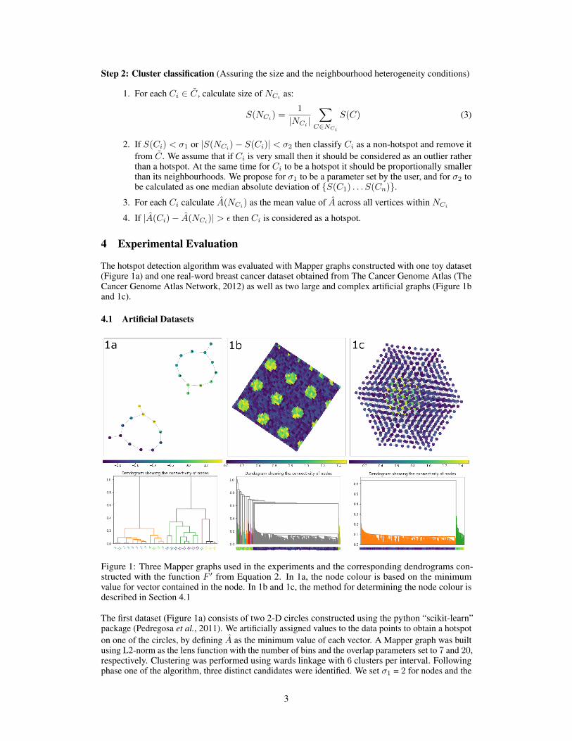
The hotspot detection algorithm was evaluated with Mapper graphs constructed with one toy dataset(Figure 1a) and one real-word breast cancer dataset obtained from The Cancer Genome Atlas (TheCancer Genome Atlas Network, 2012) as well as two large and complex artificial graphs (Figure 1band 1c).

4.1 Artificial Datasets

Figure 1: Three Mapper graphs used in the experiments and the corresponding dendrograms con-structed with the function F ′ from Equation 2. In 1a, the node colour is based on the minimumvalue for vector contained in the node. In 1b and 1c, the method for determining the node colour isdescribed in Section 4.1

The first dataset (Figure 1a) consists of two 2-D circles constructed using the python “scikit-learn”package (Pedregosa et al., 2011). We artificially assigned values to the data points to obtain a hotspoton one of the circles, by defining A as the minimum value of each vector. A Mapper graph was builtusing L2-norm as the lens function with the number of bins and the overlap parameters set to 7 and 20,respectively. Clustering was performed using wards linkage with 6 clusters per interval. Followingphase one of the algorithm, three distinct candidates were identified. We set σ1 = 2 for nodes and the

3

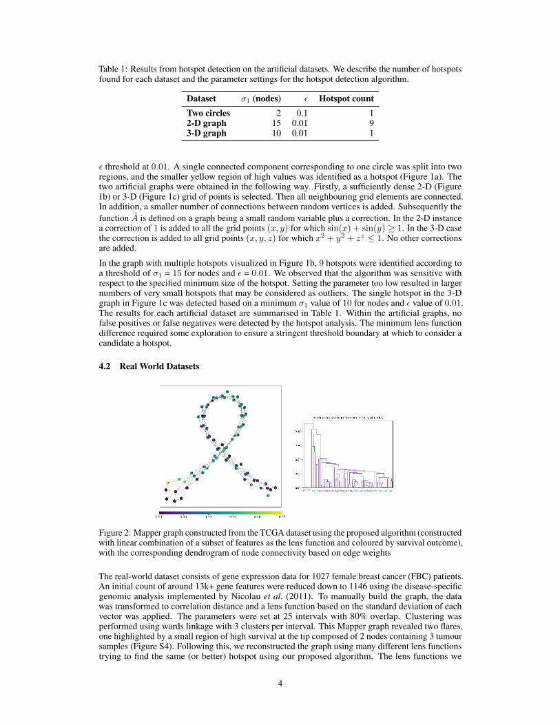
Table 1: Results from hotspot detection on the artificial datasets. We describe the number of hotspotsfound for each dataset and the parameter settings for the hotspot detection algorithm.

Dataset σ1 (nodes) ε Hotspot countTwo circles 2 0.1 12-D graph 15 0.01 93-D graph 10 0.01 1

ε threshold at 0.01. A single connected component corresponding to one circle was split into tworegions, and the smaller yellow region of high values was identified as a hotspot (Figure 1a). Thetwo artificial graphs were obtained in the following way. Firstly, a sufficiently dense 2-D (Figure1b) or 3-D (Figure 1c) grid of points is selected. Then all neighbouring grid elements are connected.In addition, a smaller number of connections between random vertices is added. Subsequently thefunction A is defined on a graph being a small random variable plus a correction. In the 2-D instancea correction of 1 is added to all the grid points (x, y) for which sin(x) + sin(y) ≥ 1. In the 3-D casethe correction is added to all grid points (x, y, z) for which x2 + y2 + zz ≤ 1. No other correctionsare added.

In the graph with multiple hotspots visualized in Figure 1b, 9 hotspots were identified according toa threshold of σ1 = 15 for nodes and ε = 0.01. We observed that the algorithm was sensitive withrespect to the specified minimum size of the hotspot. Setting the parameter too low resulted in largernumbers of very small hotspots that may be considered as outliers. The single hotspot in the 3-Dgraph in Figure 1c was detected based on a minimum σ1 value of 10 for nodes and ε value of 0.01.The results for each artificial dataset are summarised in Table 1. Within the artificial graphs, nofalse positives or false negatives were detected by the hotspot analysis. The minimum lens functiondifference required some exploration to ensure a stringent threshold boundary at which to consider acandidate a hotspot.

4.2 Real World Datasets

Figure 2: Mapper graph constructed from the TCGA dataset using the proposed algorithm (constructedwith linear combination of a subset of features as the lens function and coloured by survival outcome),with the corresponding dendrogram of node connectivity based on edge weights

The real-world dataset consists of gene expression data for 1027 female breast cancer (FBC) patients.An initial count of around 13k+ gene features were reduced down to 1146 using the disease-specificgenomic analysis implemented by Nicolau et al. (2011). To manually build the graph, the datawas transformed to correlation distance and a lens function based on the standard deviation of eachvector was applied. The parameters were set at 25 intervals with 80% overlap. Clustering wasperformed using wards linkage with 3 clusters per interval. This Mapper graph revealed two flares,one highlighted by a small region of high survival at the tip composed of 2 nodes containing 3 tumoursamples (Figure S4). Following this, we reconstructed the graph using many different lens functionstrying to find the same (or better) hotspot using our proposed algorithm. The lens functions we

4

Table 2: The results of hotspot detection on the TCGA FBC dataset. We describe the composition ofeach hotspot found for the various Mapper graphs constructed. "STD" refers to the manually createdMapper graph with a lens function built on standard deviation. Linear, linear subset, and non-linearsubset refers to the three graphs constructed using the hotspot detection algorithm.

Lens STD Linear Linear subset Non-linear subsetn 3 51 21 49Survived (%) 100 98.04 100 100ER+ (%) 0 33.33 95.24 85.71ER- (%) 100 66.67 4.76 14.29Basal (%) 100 41.18 0 6.12Her2 (%) 0 23.53 4.76 4.08LumA (%) 0 19.61 38.10 65.31Normal (%) 0 7.84 0.00 16.33LumB (%) 0 7.84 57.14 8.16

used were randomly generated as described in Section S1.3. For each scenario we ran the process(sampling of lens+Mapper+hotspot detection) 1000 times. As a criteria for hotspot detection weset the σ1 at 5 for nodes, σ1 at 10 for samples and ε at 0.15. For each type of lens function, out of1000 runs, we were able to find at least one graph with a hotspot region of increased survival. Ouroptimum result is shown in Figure 2. The composition of each hotspot is described in Table 2.

The manually created graph has a hotspot (Figure S4) consisting of 3 ER- Basal patients (0.29%of total cohort). Basal is a well-known subtype in breast cancer predicting poor survival prognosisand can easily be identified using standard hierarchical clustering (Parker et al., 2009). Our hotspotdetection method was found to locate higher numbers of patients with increased survival in a singlehotspot than the one presented in Figure S4. When comparing the identity of patients, we foundthere was no overlap between the the manually created hotspot and the hotspots identified by ouralgorithm. Both the linear (Figure S5) and non-linear subset (Figure S6) lens functions detected 51and 49 patients each respectively, but these were both determined to contain a mixture of ER statusand breast cancer subtypes. The linear subset (Figure 2) lens function contained a reduced number ofsamples, totalling 21 patients (2.05% of the full cohort). Ninety-five percent of this patient hotspot(n=20) were found to have an ER+ status, and consisted solely of Her2, LumA, and LumB subtypes.This indicates an unusual cluster of patients similar to that found in Nicolau et al. (2011).

5 Conclusion

In this paper we proposed a new method for hotspot detection on Mapper graph. This method could,for example, support biomedical analysis for precision medicine, where it is important to identifysmall groups of distinct patients that may exhibit varying behaviour. We demonstrated that themethod worked well with three artificial Mapper graphs. Furthermore, for the TCGA real worlddataset, the algorithm allowed us to construct lens functions, which led to graphs with hotspots. Tofurther evaluate the algorithm, we will biologically validate the quality of the retrieved hotspots andinvestigate the presence of these hotspots in a secondary female breast cancer dataset. As a futuredirection for this work we will explore the problem of overfitting while sampling from a space oflenses with the objective of hotspot detection.

References

Carriere, M. and Oudot, S. (2018). Structure and stability of the one-dimensional mapper. Foundations of Computational Mathematics, 18(6),1333–1396.

Cho, H. J., Zhao, J., Jung, S. W., Ladewig, E., Kong, D.-S., Suh, Y.-L., Lee, Y., Kim, D., Ahn, S. H., Bordyuh, M., et al. (2019). Distinctgenomic profile and specific targeted drug responses in adult cerebellar glioblastoma. Neuro-oncology, 21(1), 47–58.

Lum, P. Y., Singh, G., Lehman, A., Ishkanov, T., Vejdemo-Johansson, M., Alagappan, M., Carlsson, J., and Carlsson, G. (2013). Extractinginsights from the shape of complex data using topology. Scientific reports, 3, 1236.

Nicolau, M., Levine, A. J., and Carlsson, G. (2011). Topology based data analysis identifies a subgroup of breast cancers with a uniquemutational profile and excellent survival. Proceedings of the National Academy of Sciences, 108(17), 7265–7270.

5

Parker, J. S., Mullins, M., Cheang, M. C., Leung, S., Voduc, D., Vickery, T., Davies, S., Fauron, C., He, X., Hu, Z., et al. (2009). Supervisedrisk predictor of breast cancer based on intrinsic subtypes. Journal of clinical oncology, 27(8), 1160.

Pedregosa, F., Varoquaux, G., Gramfort, A., Michel, V., Thirion, B., Grisel, O., Blondel, M., Prettenhofer, P., Weiss, R., Dubourg, V., Vander-plas, J., Passos, A., Cournapeau, D., Brucher, M., Perrot, M., and Duchesnay, E. (2011). Scikit-learn: Machine learning in Python. Journalof Machine Learning Research, 12, 2825–2830.

Singh, G., Mémoli, F., and Carlsson, G. E. (2007). Topological methods for the analysis of high dimensional data sets and 3d object recognition.SPBG, 91, 100.

The Cancer Genome Atlas Network (2012). Comprehensive molecular portraits of human breast tumours. Nature, 490(7418), 61.

S1 Supplementary Material

S1.1 Definition of Mapper algorithm

In this section we introduce the Mapper algorithm originally introduced in Singh et al. (2007). Forthe convenience, the parameters of the algorithm are denoted with boldface.

Let X = {x1, . . . , xk}, xi ∈ Rn be the considered point cloud and and A : X → R indicate theattribute of data (e.g. survival of patients). In addition let us consider a lens function f : X → Rn.Typically n = 1 are used. Let us take the range of f(X) and cover it with n intervals that overlapon k percentage of their length. For instance, if f(X) = [0, 1], n=4 and k=20%, the coverage willconsist of the following four intervals of a length 5

17 : [0, 517 ], [

417 ,

917 ], [

817 ,

1317 ] and [ 1217 , 1]. Now, take

any interval I from the coverage of f(X) and consider f−1(I) = {x ∈ X|f(x) ∈ I}. We run aclustering algorithm of our choice at f−1(I) and obtain a collection of clusters CI

1 , . . . , CIm. They

will correspond to vertices of the Mapper graph. Given two intervals I, J covering f(X), two verticesv1, v2 corresponding to clusters CI

i and CJk will be joined by an edge if and only if CI

i ∩ CJk 6= ∅.

The vertices and edges defined above constitute the Mapper graph G = (V,E). We now define afunction A : V → R as:

A(v) =1

|v|∑x∈v

A(x) (4)

where A(x) is the value of the attribute.

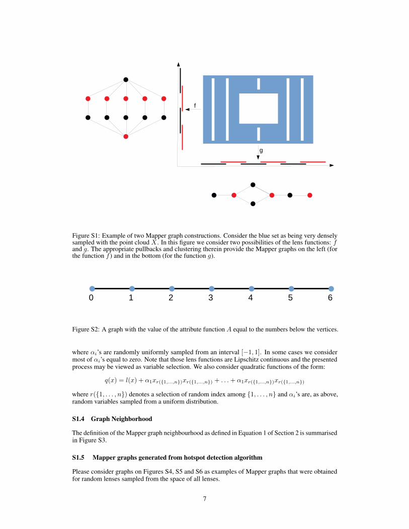
A simple illustration of the presented construction can be found in the Figure S1.

Note that the example in the Figure S1 highlights that different choices of lens functions may providevery different Mapper graphs. It is a natural phenomena, as the lens functions determine which detailsof the image are being neglected.

S1.2 Non uniqueness of components satisfying internal homogeneity criteria

The internal homogeneity criteria states that the value of the attribute function A for any two verticeswithin a proposed region should not differ more than a chosen parameter τ . Let us consider a graphtogether with the attribute function presented at Fig. S2.

For a choice of τ = k, for k ∈ {1, . . . , 6}, any connected subset of k vertices satisfy the internalhomogeneity condition. In such a case, an arbitrary subset is chosen in our algorithm.

S1.3 Sampling from a space of lenses

Selection of lenses is often a nontrivial process. For data embedded to Rn, the space of all possiblefunctions is huge. Typically the considered lenses are constructed based on expert’s opinion on thematter - on the knowledge that certain aspects of the data can be ignored (and therefore being put intofibers of the lenses). Still, in typical application, a number of lenses need to be considered before theone that is suitable for analysis is found.

The hotspot location procedures discussed in the Section 3 opens a possibility of automaticallysampling lens f from the space of possible lenses and testing the quality of f . In this instance, thelenses giving cleaner hotspots will be considered better.

In this instance, given the point cloud X ⊂ Rn and (x1, . . . , xn) ∈ X we consider random linearand quadratic functions of x. More precisely the considered linear functions are of the form:

l(x) = α1x1 + α2x2 + . . .+ αnxn

6

f

g

Figure S1: Example of two Mapper graph constructions. Consider the blue set as being very denselysampled with the point cloud X . In this figure we consider two possibilities of the lens functions: fand g. The appropriate pullbacks and clustering therein provide the Mapper graphs on the left (forthe function f ) and in the bottom (for the function g).

0 1 2 3 4 5 6

Figure S2: A graph with the value of the attribute function A equal to the numbers below the vertices.

where αi’s are randomly uniformly sampled from an interval [−1, 1]. In some cases we considermost of αi’s equal to zero. Note that those lens functions are Lipschitz continuous and the presentedprocess may be viewed as variable selection. We also consider quadratic functions of the form:

q(x) = l(x) + α1xr({1,...,n})xr({1,...,n}) + . . .+ α1xr({1,...,n})xr({1,...,n})

where r({1, . . . , n}) denotes a selection of random index among {1, . . . , n} and αi’s are, as above,random variables sampled from a uniform distribution.

S1.4 Graph Neighborhood

The definition of the Mapper graph neighbourhood as defined in Equation 1 of Section 2 is summarisedin Figure S3.

S1.5 Mapper graphs generated from hotspot detection algorithm

Please consider graphs on Figures S4, S5 and S6 as examples of Mapper graphs that were obtainedfor random lenses sampled from the space of all lenses.

7

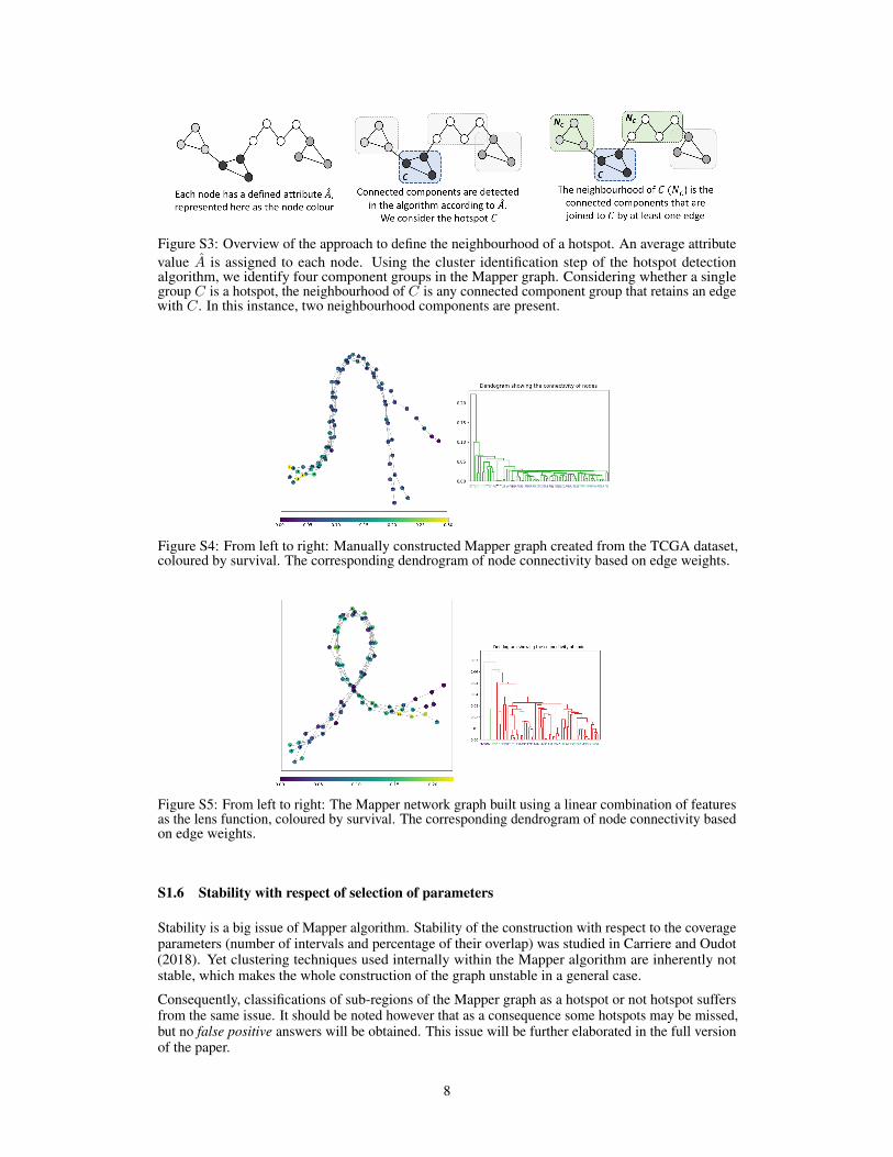
Figure S3: Overview of the approach to define the neighbourhood of a hotspot. An average attributevalue A is assigned to each node. Using the cluster identification step of the hotspot detectionalgorithm, we identify four component groups in the Mapper graph. Considering whether a singlegroup C is a hotspot, the neighbourhood of C is any connected component group that retains an edgewith C. In this instance, two neighbourhood components are present.

Figure S4: From left to right: Manually constructed Mapper graph created from the TCGA dataset,coloured by survival. The corresponding dendrogram of node connectivity based on edge weights.

Figure S5: From left to right: The Mapper network graph built using a linear combination of featuresas the lens function, coloured by survival. The corresponding dendrogram of node connectivity basedon edge weights.

S1.6 Stability with respect of selection of parameters

Stability is a big issue of Mapper algorithm. Stability of the construction with respect to the coverageparameters (number of intervals and percentage of their overlap) was studied in Carriere and Oudot(2018). Yet clustering techniques used internally within the Mapper algorithm are inherently notstable, which makes the whole construction of the graph unstable in a general case.

Consequently, classifications of sub-regions of the Mapper graph as a hotspot or not hotspot suffersfrom the same issue. It should be noted however that as a consequence some hotspots may be missed,but no false positive answers will be obtained. This issue will be further elaborated in the full versionof the paper.

8

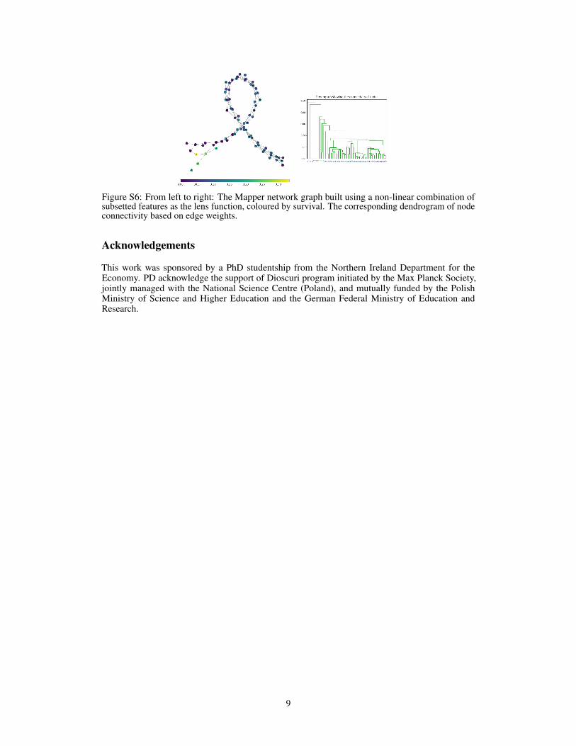
Figure S6: From left to right: The Mapper network graph built using a non-linear combination ofsubsetted features as the lens function, coloured by survival. The corresponding dendrogram of nodeconnectivity based on edge weights.

Acknowledgements

This work was sponsored by a PhD studentship from the Northern Ireland Department for theEconomy. PD acknowledge the support of Dioscuri program initiated by the Max Planck Society,jointly managed with the National Science Centre (Poland), and mutually funded by the PolishMinistry of Science and Higher Education and the German Federal Ministry of Education andResearch.

9