Embed Size (px)
Citation preview
IDEALIZED LARGE-EDDY SIMULATION SENSITIVITY
STUDIES OF SEA AND LAKE BREEZES
by
Erik T. Crosman
A dissertation submitted to the faculty ofThe University of Utah
in partial fulfillment of the requirements for the degree of
Doctor of Philosophy
Department of Atmospheric Sciences
The University of Utah
May 2011

Copyright © Erik T. Crosman 2011
All Rights Reserved

T h e U n i v e r s i t y o f U t a h G r a d u a t e S c h o o l
STATEMENT OF DISSERTATION APPROVAL
The dissertation of Erik T. Crosman
has been approved by the following supervisory committee members:
John D. Horel , Chair 10/7/2010Date Approved
Steven K. Krueger , Member 10/7/2010Date Approved
Courtenay Strong , Member 10/7/2010Date Approved
C. David Whiteman , Member 10/7/2010Date Approved
James R. Stoll , Member 10/7/2010Date Approved
and by William James Steenburgh , Chair of
the Department of Atmospheric Sciences
and by Charles A. Wight, Dean of The Graduate School.

ABSTRACT
Numerical studies of sea and lake breezes are reviewed and gaps in our current
understanding of these thermally-driven circulations are discussed. A numerical
sensitivity study is conducted using large-eddy simulations to determine the dependence
of sea- and lake-breeze speed and length scales to variations in the land-surface sensible
heat flux, offshore background wind, initial atmospheric stability, and lake diameter.
This study is the first to test the dependence of sea- and lake-breeze characteristics to
variations in these geophysical variables using a three-dimensional large-eddy simulation
capable of explicitly resolving boundary-layer turbulence and vertical motion near the
sea-breeze front.
This study provides new understanding on the sensitivity of sea and lake breezes to
variations in the land-surface sensible heat flux, opposing background wind, and lake
diameter as well as the complex interactions that occur among these geophysical
variables. For the first time, the daytime life cycle of sea and lake breezes in the presence
of variations in these variables is simulated, in contrast to many earlier studies that
focused primarily on the mature midafternoon sea-breeze circulation. Significant spatial
variability in the intensity and vertical structure of lake and sea breezes is noted in the
large-eddy simulations. The critical value of an opposing wind at which a sea or lake
breeze is destroyed by synoptic-scale pressure gradients is approximately 20% lower in
this study than that documented in earlier numerical studies. The depth of sea and lake
iii
breezes has also been found to be highly sensitive to the magnitude of the opposing
background wind. Finally, the results of this study show that lake breezes for small and
medium-sized lakes evolve much differently than sea breezes during the afternoon due to
a limited quantity of cool air over the lake.
iv
TABLE OF CONTENTS
ABSTRACT.......................................................................................................................iii
ACKNOWLEDGEMENTS................................................................................................vi
CHAPTERS
1 INTRODUCTION.........................................................................................................1
2 SEA AND LAKE BREEZES: A REVIEW OF NUMERICAL STUDIES..................3
Abstract....................................................................................................................3Introduction..............................................................................................................3History of Numerical Studies of Sea Breezes..........................................................8Sensitivity Studies of Temporally-dependent Geophysical Variables...................11Sensitivity Studies of Location-dependent Geophysical Variables.......................28Discussion..............................................................................................................36
3 LARGE-EDDY SIMULATION OF A SEA BREEZE...............................................48
Motivation and Background..................................................................................48Weather and Forecasting Model as a Large-Eddy Simulation..............................50Model Set-up for Control Simulation...................................................................53
Control Simulation................................................................................................57
4 NUMERICAL SENSITIVITY STUDIES...................................................................63
Overview................................................................................................................63 Sensitivity to the Land-Surface Sensible Heat Flux..............................................68
Sensitivity to the Initial Atmospheric Stability......................................................72Sensitivity to the Offshore Background Wind.......................................................74Sensitivity to Lake Diameter.................................................................................93
5 SUMMARY AND FUTURE WORK......................................................................105
Sensitivity to Geophysical Variables...................................................................105Future Work.........................................................................................................111
REFERENCES................................................................................................................113
v

ACKNOWLEDGEMENTS
I would like to thank my advisor, John Horel, for his endless patience, vision, and guidance. I would also like to thank my other four committee members, C. David Whiteman, Steven Krueger, James (Rob) Stoll, and Courtenay Strong, for their valuable comments and expertise. I am also very appreciative of the support and advice given to me by Vince Salomonson over the last several years.
An allocation of computer time from the Center for High Performance Computing at the University of Utah is gratefully acknowledged and made this study possible. Thanks also goes to the Center for High Performance Computing support personnel, as well as Martin Cuma, Jimy Dudhia, Rich Rotunno, and Song-Lak Kang for their assistance with the WRF model and Dan Tyndall for solving many miscellaneous technical problems. Thanks also goes to University of Utah undergraduate students who volunteered their time as part of a field study on the Great Salt Lake breeze: Cody Oppermann, Liz Looby, Keira Harper, Brad Sorensen, Gary Vardon, Wil Mace, James Judd, Tricia Oliphant, Martin Schroeder, and Jonathan Tippetts.
This research was primarily supported by the National Science Foundation project entitled “Lake Breeze System of the Great Salt Lake” Grant # ATM-0802282. Some funding was also provided by a NASA Earth System Science Fellowship (08-Earth08R-5).
CHAPTER 1
INTRODUCTION
Sea and lake breezes have been studied extensively using both observational and
numerical approaches (Simpson et al. 1994; Miller et al. 2003). However, the spatially
and temporally varying characteristics of sea- and lake-breeze evolution and their effects
on air pollutant transport and wind power resources remain active areas of research (e.g.,
Levy et. al. 2009; Shaw et al. 2009). The continued interest in sea breezes is in large part
due to the ubiquity of sea breezes in highly-populated coastal regions, the importance of
sea breezes to coastal air-quality and wind energy interests, and the sensitivity of sea and
lake breezes to anthropogenic and natural land-use changes. A number of questions
remain regarding the sea-breeze life cycle and dependence on geophysical variables. For
example, the development of offshore wind farms requires better understanding of the
sea-breeze life cycle in the largely unstudied offshore region. In addition, lake breezes,
which are notably different than sea breezes for small to medium-sized lakes, have not
been studied rigorously either numerically or observationally. As lakes shrink and coastal
vegetation regimes change due to anthropogenic global warming, the corresponding
changes in sea- and lake-breeze intensity are unclear. This study seeks to improve the
understanding of how variations in the land-surface sensible heat flux, initial atmospheric
stability, offshore background wind, and water body diameter influence sea and lake
breezes. These questions are best answered numerically as observational approaches are
2
severely limited by the spatially inhomogeneous and temporally-varying natural
environment. In addition, the entire vertical and horizontal structure of the sea-breeze
circulation, which can extend over 100 km horizontally and over 3 km vertically, can
rarely be observed from in situ observations typically focused on the near-ground, near-
coast environment.
This study is organized as follows. A review on previous numerical modeling studies
of sea and lake breezes is presented in Chapter 2 with the goal of determining the current
understanding of sea and lake breezes obtained from over 50 years of numerical
modeling and those aspects of sea and lake breezes that require additional understanding.
The methodology of using the Weather Research and Forecasting (WRF) model as a
large-eddy simulation for studying sea and lake breezes is presented in Chapter 3, along
with the control simulation. Results from 50 large-eddy simulations testing the
dependence of sea and lake breezes to variations in the land-surface sensible heat flux,
initial atmospheric stability, offshore background wind, and water body diameter are
presented in Chapter 4. A summary and outline of future work is given in Chapter 5.

CHAPTER 2
SEA AND LAKE BREEZES: A REVIEW OF NUMERICAL STUDIES
Abstract
Numerical studies of sea and lake breezes are reviewed. The modeled dependence of sea-
breeze and lake-breeze characteristics on the land surface sensible heat flux, ambient
geostrophic wind, atmospheric stability and moisture, water body dimensions, terrain
height and slope, Coriolis parameter, surface roughness length, and shoreline curvature is
discussed. Consensus results on the influence of these geophysical variables on sea and
lake breezes are synthesized as well as current gaps in our understanding. A brief history
of numerical modeling, an overview of recent high-resolution simulations, and
suggestions for future research related to sea and lake breezes are also presented. The
results of this survey are intended to be a resource for numerical modeling, coastal air
quality, and wind power studies.
Introduction
Sea, gulf, lake, and river breezes are local circulations driven by differential heating
between land and water. The basic dynamics and properties of these thermally-driven
systems, hereafter referred to collectively as sea breezes (SB), have been studied
extensively since the 1950s and are well understood (Simpson 1994; Miller et al. 2003).
Sea breezes are of interest because of their ubiquity around the world, their recurring and
4
well-defined features that lend themselves to examination using a variety of analytic,
observational, and numerical approaches, and their societal impacts. For example, land-
use changes and rapid population growth in coastal regions (with projections of 75% of
the world’s population to be located in those areas by 2030) may lead to a significant
degradation of coastal air quality in many areas, with that degradation modulated by sea
breezes (Hinrichsen 1999; Levy et al. 2008; 2009).
Although the overall structure, life cycle, and forecasting of sea breezes have been
reviewed extensively (e.g., Atkinson 1981; Pielke and Segal 1986; Abbs and Physick
1992; Simpson 1994; Segal et al. 1997; Miller et al. 2003), there has not been a review
dedicated to the results from over 50 years of numerical modeling of sea breezes. The
main focus of this survey concerns the modeled dependence of sea breezes on ten
geophysical variables: the land surface sensible heat flux (H, which establishes the land-
sea temperature difference), ambient geostrophic wind (Vg), atmospheric stability (N),
atmospheric moisture (q), water body dimensions (d), terrain height (ht), terrain slope (s),
Coriolis parameter (f), surface aerodynamic roughness length (zo), and shoreline
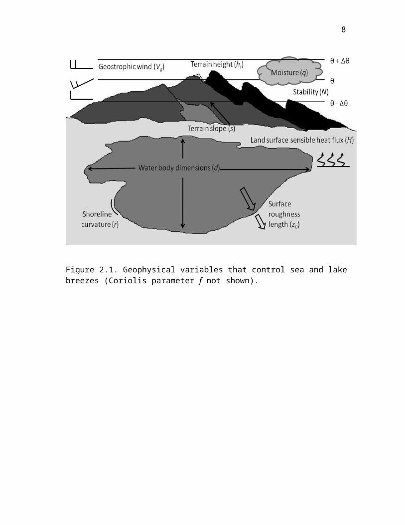
curvature (r) (Fig. 2.1). Four of these variables vary significantly over time at a given
location as a function of season, soil moisture content, and atmospheric state (H, Vg, N,
and q) while the remaining six are largely temporally invariant at any given location (d,
ht, s, f, zo, and r).
The spatial and temporal scales and quasi-regularity of SB have provided a modeling
framework for performing sensitivity experiments in which one or more variables are
perturbed. The effects of the variables on the characteristics of sea breezes are discussed
in terms of four widely-used measures of thermally-driven circulation intensity: the
5
Figure 2.1. Geophysical variables that control sea and lake breezes (Coriolis parameter f not shown).
6
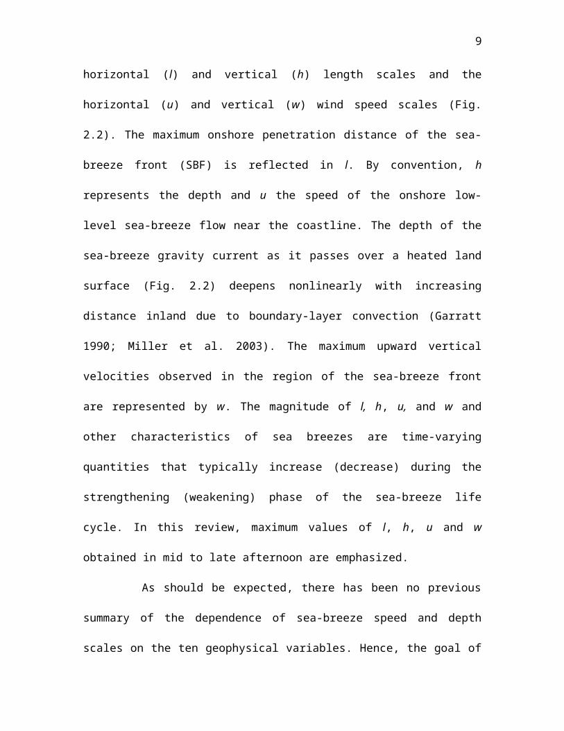
horizontal (l) and vertical (h) length scales and the horizontal (u) and vertical (w) wind
speed scales (Fig. 2.2). The maximum onshore penetration distance of the sea-breeze
front (SBF) is reflected in l. By convention, h represents the depth and u the speed of the
onshore low-level sea-breeze flow near the coastline. The depth of the sea-breeze gravity
current as it passes over a heated land surface (Fig. 2.2) deepens nonlinearly with
increasing distance inland due to boundary-layer convection (Garratt 1990; Miller et al.
2003). The maximum upward vertical velocities observed in the region of the sea-breeze
front are represented by w. The magnitude of l, h, u, and w and other characteristics of
sea breezes are time-varying quantities that typically increase (decrease) during the
strengthening (weakening) phase of the sea-breeze life cycle. In this review, maximum
values of l, h, u and w obtained in mid to late afternoon are emphasized.
As should be expected, there has been no previous summary of the dependence of
sea-breeze speed and depth scales on the ten geophysical variables. Hence, the goal of
this review is to piece together the results from, and the agreement among, the many
numerical studies. A limited review of observational studies is also included to ascertain
the realism of the numerical simulations. Gaps in our understanding and
recommendations for future research are also presented.
Although likely the most thorough review of numerical studies of sea breezes to date,
it is far from comprehensive. The following topics are not extensively discussed:
pollutant dispersion models (Clappier et al. 2000; Melas et al. 2006), land-surface models
(Cheng and Byun 2008), linear and analytical models (Rotunno 1983; Niino 1987; Dalu
and Pielke 1989; Qian et al. 2009; Drobinski and Dubos 2009), laboratory experiments
7
(Simpson 1997; Cenedese et al. 2000; Hara et al. 2009), land breezes (Buckley and

8
Kurzeja 1997), and convective internal boundary-layer growth (Garratt 1990; Kuwagata
et al. 1994; Levitin and Kambezidis 1997; Liu et al. 2001; Miller et al. 2003).
History of Numerical Studies of Sea Breezes
Numerical simulations of sea breezes require solving the equations of motion for the
conservation of mass, momentum, and energy. Model physics (e.g., surface processes,
radiation, latent heating, and turbulent diffusion of heat, moisture, and momentum) and
model dynamics (horizontal advection, vertical acceleration, Coriolis effects, density
changes, and time-dependence) must be adequately resolved to obtain a realistic
simulation (Avissar et al. 1990). Increasingly sophisticated treatment of both model
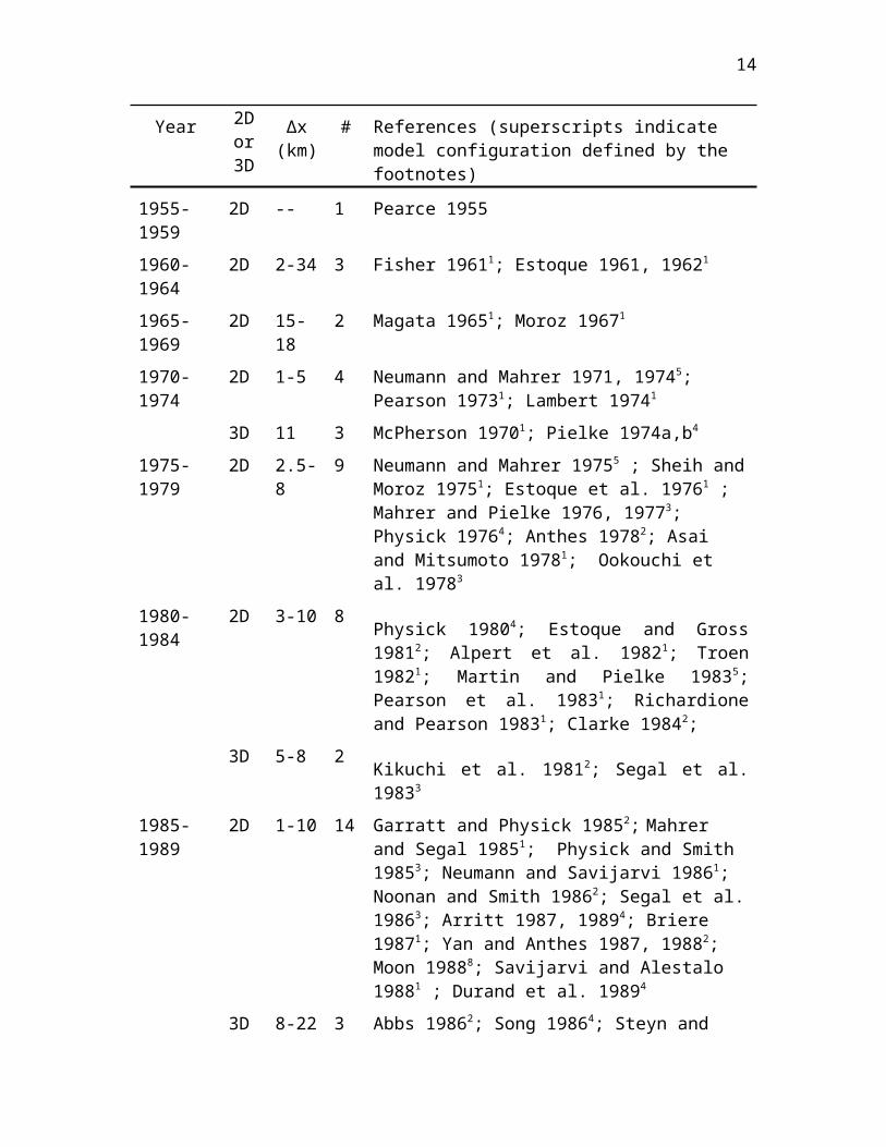
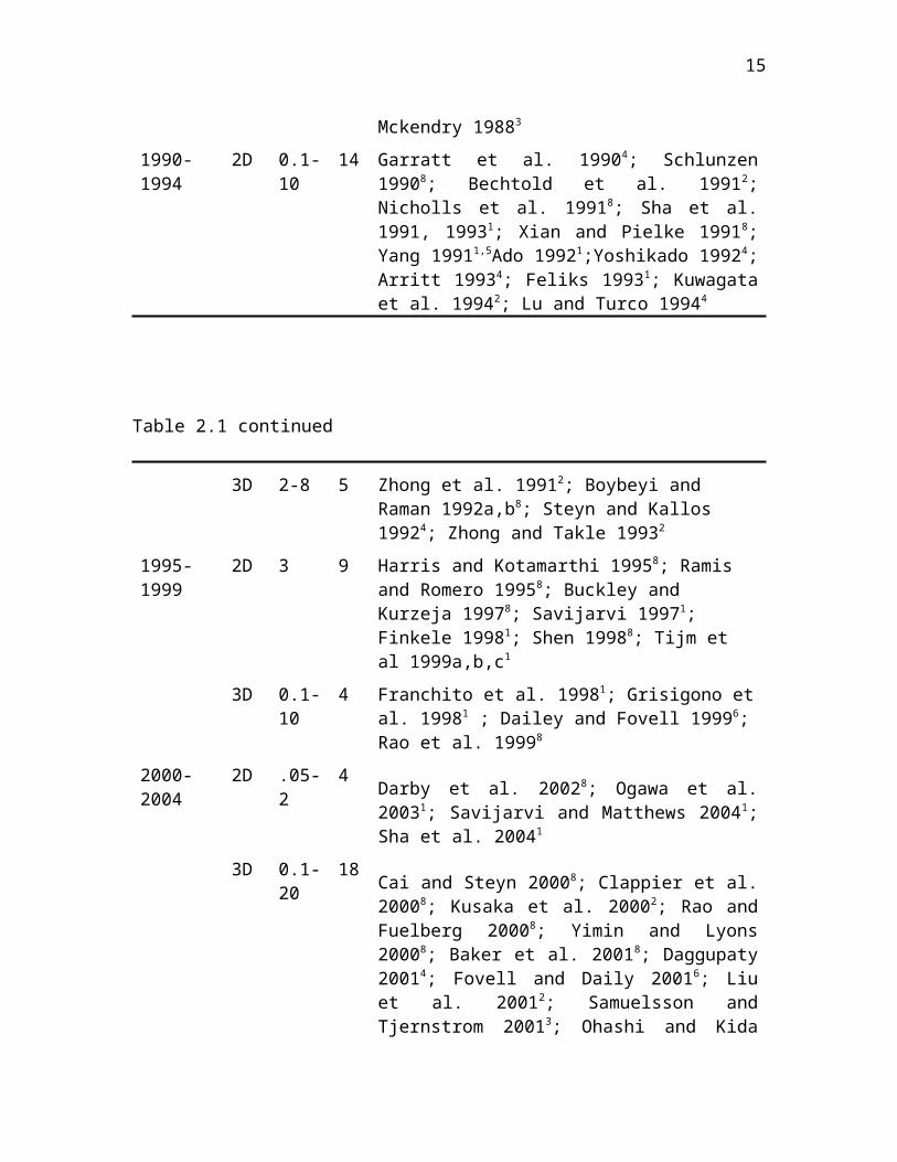
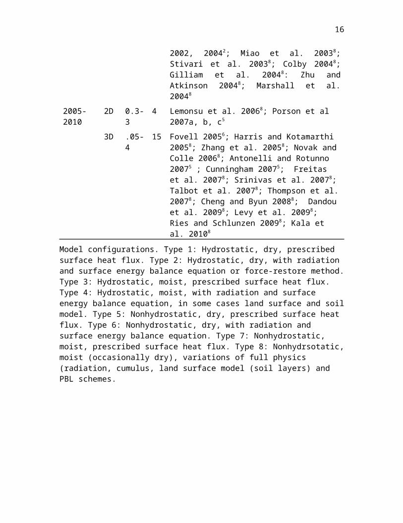
dynamics and physics has occurred over the past 50 years. Table 2.1 summarizes the
evolution of model physics, horizontal resolution, and dimension that parallels the
increase in computational speed. The earliest hydrostatic models used simple boundary-
layer schemes and neglected moisture, latent heating, radiation, and land-surface
parameterizations. Some later models included radiation, moisture, and latent heating,
with increasingly sophisticated schemes for surface heating and the turbulent transport of
heat, moisture, and momentum. Through the 1970s, turbulence in the surface layer was
generally treated using simple K-theory, assuming constant fluxes, and with empirical
formulations for turbulent transport in the overlying transition layer. From around 1980
to the present day, Monin-Obukov similarity theory has been used most commonly to
derive surface layer fluxes, with prognostic turbulent kinetic energy formulations
typically used for transition layer turbulence.
Beginning with the first numerical simulation by Pearce (1955), there has been a
steady increase in the number of scientific investigations devoted to sea breezes.
9
Table 2.1: Numerical modeling studies published between 1955 and 2010 that have been reviewed as part of this study. The approximate range of horizontal spatial scales (Δx) and the total number (#) of studies during each 5-year period are provided.
Year 2D or 3D
Δx (km)
# References (superscripts indicate model configuration defined by the footnotes)
1955-1959
2D -- 1 Pearce 1955
1960-1964
2D 2-34 3 Fisher 19611; Estoque 1961, 19621
1965-1969
2D 15-18 2 Magata 19651; Moroz 19671
1970-1974
2D 1-5 4 Neumann and Mahrer 1971, 19745; Pearson 19731; Lambert 19741
3D 11 3 McPherson 19701; Pielke 1974a,b4
1975-1979
2D 2.5-8 9 Neumann and Mahrer 19755 ; Sheih and Moroz 19751; Estoque et al. 19761 ; Mahrer and Pielke 1976, 19773; Physick 19764; Anthes 19782; Asai and Mitsumoto 19781; Ookouchi et al. 19783
1980-1984
2D 3-10 8Physick 19804; Estoque and Gross 19812; Alpert et al. 19821; Troen 19821; Martin and Pielke 19835; Pearson et al. 19831; Richardione and Pearson 19831; Clarke 19842;
3D 5-8 2Kikuchi et al. 19812; Segal et al. 19833
1985-1989
2D 1-10 14 Garratt and Physick 19852; Mahrer and Segal 19851; Physick and Smith 19853; Neumann and Savijarvi 19861; Noonan and Smith 19862; Segal et al. 19863; Arritt 1987, 19894; Briere 19871; Yan and Anthes 1987, 19882; Moon 19888; Savijarvi and Alestalo 19881 ; Durand et al. 19894
3D 8-22 3 Abbs 19862; Song 19864; Steyn and Mckendry 19883
1990-1994
2D 0.1-10
14 Garratt et al. 19904; Schlunzen 19908; Bechtold et al. 19912; Nicholls et al. 19918; Sha et al. 1991, 19931; Xian and Pielke 19918; Yang 19911,5Ado 19921;Yoshikado 19924; Arritt 19934; Feliks 19931; Kuwagata et al. 19942; Lu and Turco 19944
10
Table 2.1 continued
3D 2-8 5 Zhong et al. 19912; Boybeyi and Raman 1992a,b8; Steyn and Kallos 19924; Zhong and Takle 19932
1995-1999
2D 3 9 Harris and Kotamarthi 19958; Ramis and Romero 19958; Buckley and Kurzeja 19978; Savijarvi 19971; Finkele 19981; Shen 19988; Tijm et al 1999a,b,c1
3D 0.1-10
4 Franchito et al. 19981; Grisigono et al. 19981 ; Dailey and Fovell 19996; Rao et al. 19998
2000-2004
2D .05-2 4Darby et al. 20028; Ogawa et al. 20031; Savijarvi and Matthews 20041; Sha et al. 20041
3D 0.1-20
18Cai and Steyn 20008; Clappier et al. 20008; Kusaka et al. 20002; Rao and Fuelberg 20008; Yimin and Lyons 20008; Baker et al. 20018; Daggupaty 20014; Fovell and Daily 20016; Liu et al. 20012; Samuelsson and Tjernstrom 20013; Ohashi and Kida 2002, 20042; Miao et al. 20038; Stivari et al. 20038; Colby 20048; Gilliam et al. 20048: Zhu and Atkinson 20048; Marshall et al. 20048
2005-2010
2D 0.3-3 4 Lemonsu et al. 20068; Porson et al 2007a, b, c5
3D .05-4 15 Fovell 20056; Harris and Kotamarthi 20058; Zhang et al. 20058; Novak and Colle 20068; Antonelli and Rotunno 20075 ; Cunningham 20075; Freitas et al. 20078; Srinivas et al. 20078; Talbot et al. 20078; Thompson et al. 20078; Cheng and Byun 20088; Dandou et al. 20098; Levy et al. 20098; Ries and Schlunzen 20098; Kala et al. 20108
Model configurations. Type 1: Hydrostatic, dry, prescribed surface heat flux. Type 2: Hydrostatic, dry, with radiation and surface energy balance equation or force-restore method. Type 3: Hydrostatic, moist, prescribed surface heat flux. Type 4: Hydrostatic, moist, with radiation and surface energy balance equation, in some cases land surface and soil model. Type 5: Nonhydrostatic, dry, prescribed surface heat flux. Type 6: Nonhydrostatic, dry, with radiation and surface energy balance equation. Type 7: Nonhydrostatic, moist, prescribed surface heat flux. Type 8: Nonhydrsotatic, moist (occasionally dry), variations of full physics (radiation, cumulus, land surface model (soil layers) and PBL schemes.
11
Of the studies listed in Table 2.1, over twice as many were devoted to sea breezes
between 1985-2004 than between 1965-1984. Most early numerical studies of sea breezes
were idealized simulations, while recent studies primarily specify initial and lateral
boundary conditions from observations.
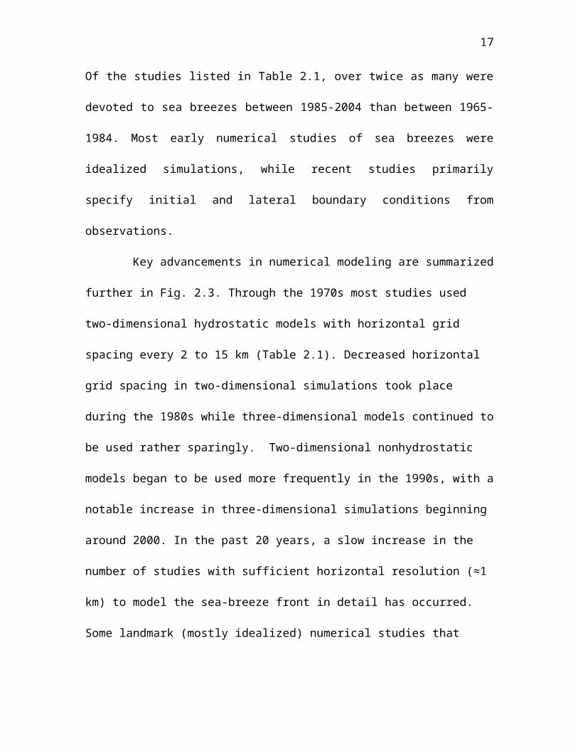
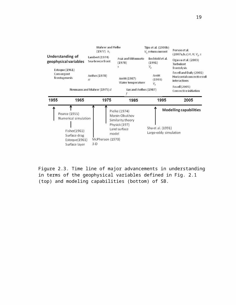
Key advancements in numerical modeling are summarized further in Fig. 2.3.
Through the 1970s most studies used two-dimensional hydrostatic models with horizontal
grid spacing every 2 to 15 km (Table 2.1). Decreased horizontal grid spacing in two-
dimensional simulations took place during the 1980s while three-dimensional models
continued to be used rather sparingly. Two-dimensional nonhydrostatic models began to
be used more frequently in the 1990s, with a notable increase in three-dimensional
simulations beginning around 2000. In the past 20 years, a slow increase in the number of
studies with sufficient horizontal resolution (≈1 km) to model the sea-breeze front in
detail has occurred. Some landmark (mostly idealized) numerical studies that improved
understanding of the effects of geophysical variables on sea breezes are summarized in
Fig. 2.3.
Sensitivity Studies of Temporally-dependent Geophysical Variables
Land-Surface Sensible Heat Flux (H)
Differential sensible heating during the daytime between land and water surfaces
results in the horizontal gradients in pressure that drive sea breezes (Steyn 2003; Kruit et
al. 2004). There is general agreement that the horizontal temperature gradient
12
Figure 2.3. Time line of major advancements in understanding in terms of the geophysical variables defined in Fig. 2.1 (top) and modeling capabilities (bottom) of SB.
13
between the water and land surface beyond the sea breeze is needed (Kruit et al. 2004),
although several scaling studies yielded superior results using horizontal temperature
gradients adjacent to the shoreline (Porson et al. 2007a; Kala et al. 2010). In any case, ΔT
is generally computed using observations near the coast, simply as a result of available
data resources (Steyn 2003).
The dependence of sea breezes on the magnitude of the land-surface sensible heat
flux (H) and the period (ω) over which the diurnal heating takes place can be seen in the
scaling relations in Table 2.2 for u and h due to Steyn (1998) and Porson et al. (2007a).
Despite this dependence, there is no consistent approach in the literature to describe time-
integrated differential sensible heating, since most numerical studies of sea breezes have
focused on dynamical, rather than thermodynamical, aspects of these systems (Kuwagata
et al. 1994). The land-surface sensible heat flux in numerical simulations is either
directly prescribed through a time-varying sinusoidal function (set to near zero over the
water surface) or indirectly specified through changes in vegetation type, soil moisture
content, or latitude. Since nearly all studies focus on summer months in the midlatitudes,
with generally a 12-hr period of diurnal heating, the maximum land-surface sensible heat
flux used in each study provides a basis for comparison and is used hereafter. Table 2.3
summarizes the key findings from studies that have examined the role of differential
sensible heating. As the fundamental driver of sea breezes, the magnitude of the land-
surface sensible heat flux influences all aspects of the circulation. The scaling analyses
summarized in Table 2.2 help to quantify the impacts of the land-surface sensible heat
flux on sea-breeze characteristics based on selected observational (Steyn 1998),
theoretical (Segal et al. 1997), and numerical (Porson et al. 2007a; Antonelli and Rotunno

14
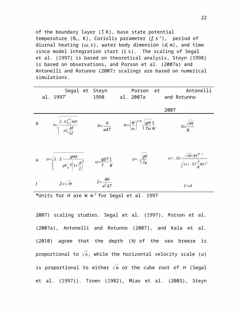
Table 2.2:A selection of recent scaling relations for sea-breeze vertical (h) and horizontal (l) length scales and horizontal velocity scale (u).Variables listed are land-surface sensible heat flux (H, K m s-1), Brunt-Vaisala frequency (N, s-1 ), vertical acceleration (g, m s-2), air density (ρ, kg m-3), temperature difference between boundary layer air over water and land (ΔT, K), reference temperature of the boundary layer (T, K), base state potential temperature (θo, K), Coriolis parameter (f, s-1), period of diurnal heating (ω, s), water body dimension (d, m), and time since model integration start (t, s). The scaling of Segal et al. (1997) is based on theoretical analysis, Steyn (1998) is based on observations, and Porson et al. (2007a) and Antonelli and Rotunno (2007) scalings are based on numerical simulations.
Segal et al. 1997* Steyn 1998 Porson et al. 2007a Antonelli and Rotunno 2007
hh=√ 2 .4∫t 1
t 2Hdt
ρC pΔθΔZ
h= HωΔT
h=(Nω )
1/6 √gHTω
1N h=√Ht
N
u u=3√1 . 2 gHd
ρC p T (1+ dl )
2 u=gΔTT
1N
u=.√ gHTω
u=.32 √ Ht (Nt )0.1
√1+(. 37 fN
Nt )2
l l∝√H l= NHω2 ΔT l≈ut
*Units for H are W m-2 for Segal et al. 1997
2007) scaling studies. Segal et al. (1997), Porson et al. (2007a), Antonelli and Rotunno
(2007), and Kala et al. (2010) agree that the depth (h) of the sea breeze is proportional to
√H , while the horizontal velocity scale (u) is proportional to either √ H or the cube root
of H (Segal et al. (1997)). Troen (1982), Miao et al. (2003), Steyn (1998), and Shen
(1998) found that h varied somewhat more strongly with H, but which may be due to
additional effects, such as a small water body dimension (Shen 1998), local complex
terrain (Miao et al. 2003), or with h defined inland from the shoreline (Troen 1982).
15
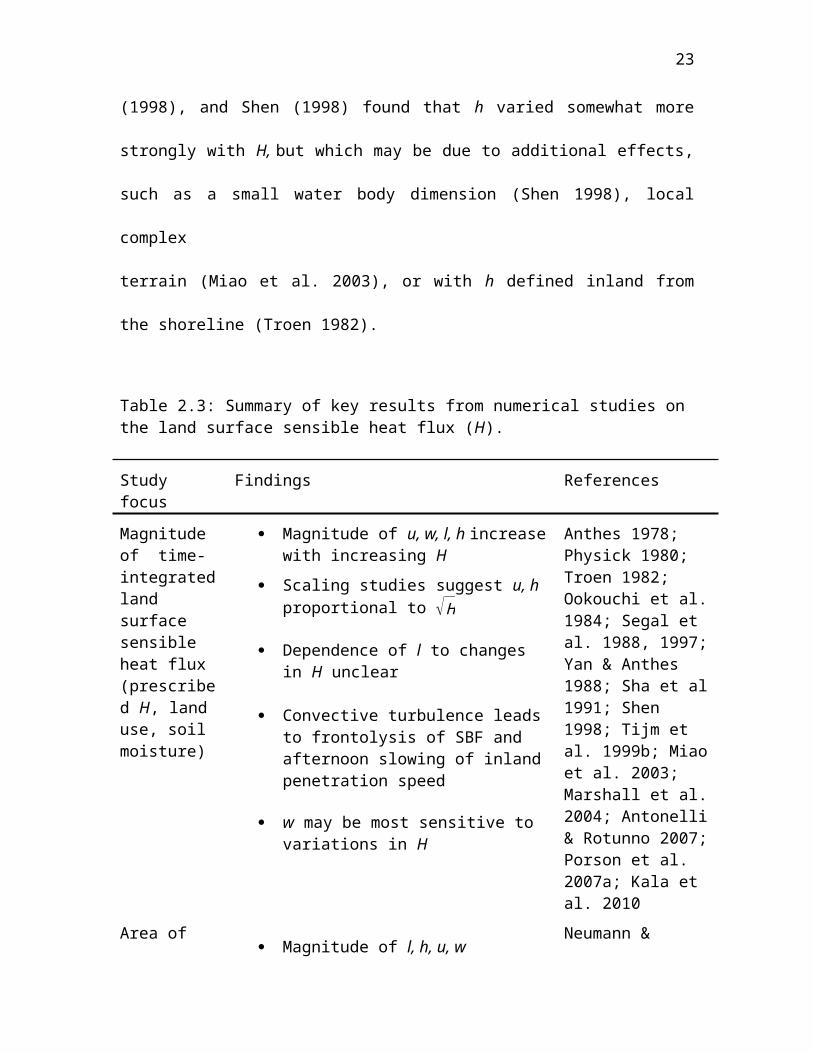
Table 2.3: Summary of key results from numerical studies on the land surface sensible heat flux (H).
Study focus Findings References
Magnitude of time-integrated land surface sensible heat flux (prescribed H, land use, soil moisture)
Magnitude of u, w, l, h increase with increasing H
Scaling studies suggest u, h proportional to √ H
Dependence of l to changes in H unclear
Convective turbulence leads to frontolysis of SBF and afternoon slowing of inland penetration speed
w may be most sensitive to variations in H
Anthes 1978; Physick 1980; Troen 1982; Ookouchi et al. 1984; Segal et al. 1988, 1997; Yan & Anthes 1988; Sha et al 1991; Shen 1998; Tijm et al. 1999b; Miao et al. 2003; Marshall et al. 2004; Antonelli & Rotunno 2007; Porson et al. 2007a; Kala et al. 2010
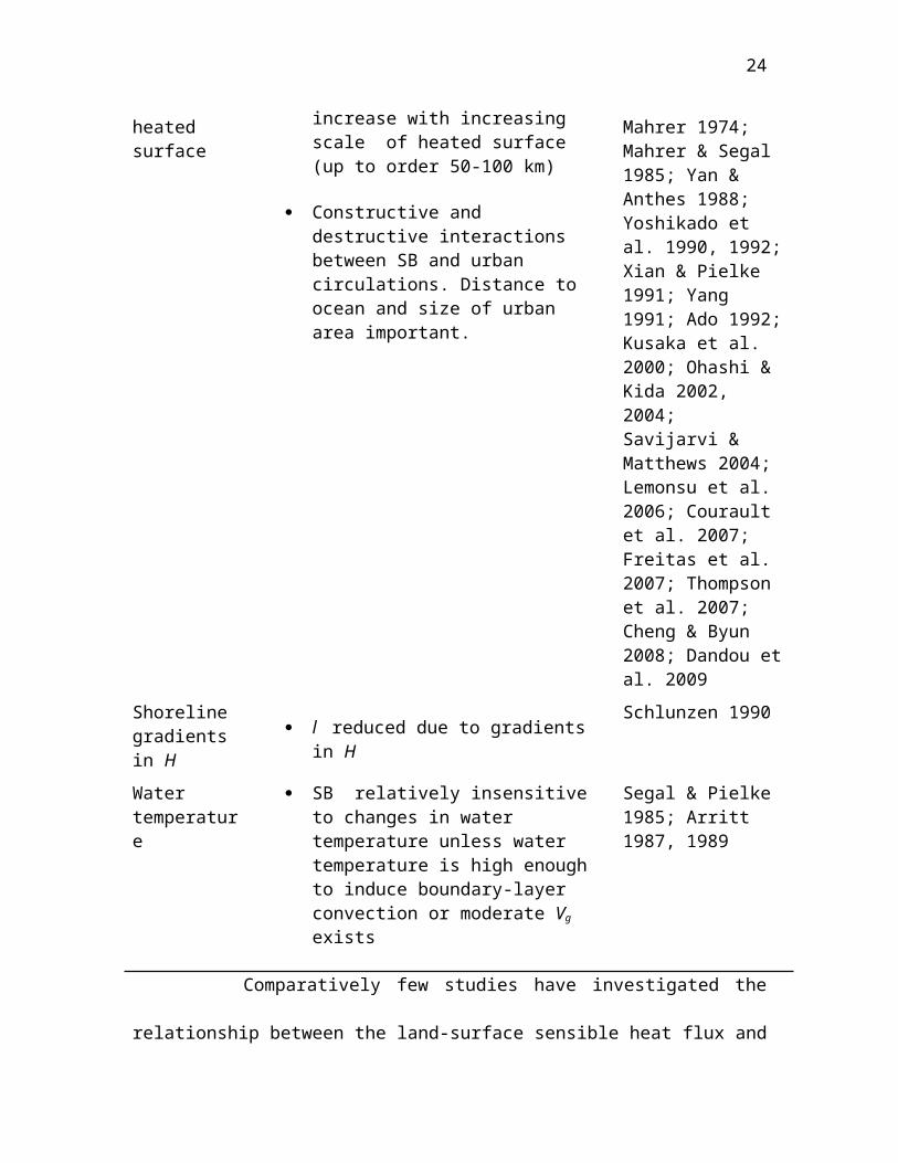
Area of heated surface Magnitude of l, h, u, w increase with
increasing scale of heated surface (up to order 50-100 km)
Constructive and destructive interactions between SB and urban circulations. Distance to ocean and size of urban area important.
Neumann & Mahrer 1974; Mahrer & Segal 1985; Yan & Anthes 1988; Yoshikado et al. 1990, 1992; Xian & Pielke 1991; Yang 1991; Ado 1992; Kusaka et al. 2000; Ohashi & Kida 2002, 2004; Savijarvi & Matthews 2004; Lemonsu et al. 2006; Courault et al. 2007; Freitas et al. 2007; Thompson et al. 2007; Cheng & Byun 2008; Dandou et al. 2009
Shoreline gradients in H l reduced due to gradients in H
Schlunzen 1990
Water temperature
SB relatively insensitive to changes in water temperature unless water temperature is high enough to induce boundary-layer convection or moderate Vg exists
Segal & Pielke 1985; Arritt 1987, 1989
16
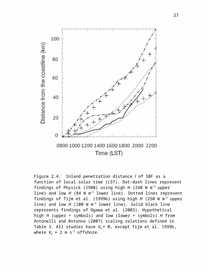
Comparatively few studies have investigated the relationship between the land-
surface sensible heat flux and the maximum inland penetration (l) and inland penetration
speed of the sea-breeze front. Fig. 2.4 summarizes the results of several numerical studies
of l as a function of the time of day and the land-surface sensible heat flux. In these
studies, high values of the land-surface sensible heat flux result in greater inland
penetration and higher penetration speeds. Although Segal et al. (1997) also show a
relatively strong variation of l with the land-surface sensible heat flux, Miao et al. (2003)
and Troen (1982) suggest less dependence. This ambiguity may arise from two opposing
tendencies. Increasing the land-surface sensible heat flux tends to increase the overall
intensity of sea breezes, which acts to increase l. However, as the land-surface sensible
heat flux increases, turbulent convection also increases, which acts to destroy the thermal
gradient along the sea-breeze front. This process, known as turbulent frontolysis,
decreases the inland penetration of the sea-breeze front through a weakening of the
horizontal temperature gradient during peak daytime heating and increasing drag
(Simpson et al. 1977; Abbs and Physick 1992; Ogawa et al. 2003).
Turbulence in the convective boundary layer has a noted effect on frontal dynamics
(Wood et al. 1999; Stephan et al. 1999; Ogawa et al. 2003). The inland penetration speed
of sea breezes typically decreases during early afternoon due to the aforementioned
turbulent frontolysis, before accelerating again during the late afternoon and evening
when turbulence diminishes. As shown in Fig. 2.4, there is a pronounced decrease in the
inland penetration speed between 1400 and 1800 local solar time (LST) with an inland
acceleration after 1800 LST for low, but not high, values of the land-surface sensible heat
flux according to Physick (1980) and Tijm et al. (1999b). Several authors
17
Figure 2.4. Inland penetration distance l of SBF as a function of local solar time (LST). Dot-dash lines represent findings of Physick (1980) using high H (240 W m-2 upper line) and low H (84 W m-2 lower line). Dotted lines represent findings of Tijm et al. (1999b) using high H (250 W m-2 upper line) and low H (100 W m-2 lower line). Solid black line represents findings of Ogawa et al. (2003). Hypothetical high H (upper + symbols) and low (lower + symbols) H from Antonelli and Rotunno (2007) scaling relations defined in Table 3. All studies have Vg = 0, except Tijm et al. 1999b, where Vg = 2 m s-1 offshore.
18
have discussed the inability of some numerical studies to reproduce the afternoon
deceleration of the sea-breeze front, presumably due to poor turbulence representation.
The numerical model of Ogawa et al. (2003) was operated with fine enough grid spacing
to simulate several periodic variations (surges) in the afternoon inland penetration speed
associated with turbulence-generated frontogenesis and frontolysis between 1400 and
1800 LST (Fig. 2.4).
The dependence of vertical motion associated with the sea-breeze front on the land-
surface sensible heat flux has been largely neglected, in part due to the inability of
hydrostatic models with horizontal grid spacing greater than 1 km to accurately simulate
this component of sea breezes. Indications are that the vertical velocity may be highly
sensitive to variations in the land-surface sensible heat flux (Troen 1982; Yang 1991;
Shen 1998; Miao et al. 2003). The effects of variations in the land-surface sensible heat
flux on offshore compensatory subsidence associated with sea breezes have not been
thoroughly investigated, although Shen (1998) found that vertical motions in the
subsidence zone over a small lake were relatively insensitive to variations in the land-
surface sensible heat flux.
Several other aspects of the dependence of sea breezes to the land-surface sensible
heat flux have been investigated, including the size of the heated land surface (Xian and
Pielke 1991; Savijarvi and Matthews 2004). Neumann and Mahrer (1974), Mahrer and
Segal (1985), and Yan and Anthes (1988) found that as the spatial extent of heating
increases (up to ≈ 50-100 km), sea breezes tend to become stronger and deeper (i.e.,
small islands or strips of land have weaker sea breezes than their larger counterparts).
However, Yang (1991) found that sea breezes were less developed for increasingly larger
19
heating scales. Schlunzen (1990) concluded that horizontal gradients in the land-surface
sensible heat flux affect l more than u and w.
Sea-breeze characteristics may also be weakened or strengthened by interactions
(e.g., frictional retardation, thermal coupling) with an urban heat island circulation. The
size of the urban area, distance between the urban area and the coast, and surrounding
topography modulate these highly variable (in both sign and magnitude) interactions
(Yoshikado 1990, 1992; Ado 1992; Kusaka et al. 2000; Ohashi and Kida 2002; 2004;
Lemonsu et al. 2006; Freitas et al. 2007; Thompson et al. 2007; Cheng and Byun 2008;
Dandou et al. 2009).
Although most studies specify constant values of water surface temperature,
variations in water temperature have been shown to influence both sea and lake breezes
(Segal and Pielke 1985; Arritt 1987; Franchito et al. 1998; 2008). Segal and Pielke
(1985) found that lake temperature had a small effect on the lake breeze except in the
case that included a moderate geostrophic wind. Arritt (1987) found negligible effects on
the lake breeze as well until lake temperature was increased sufficiently to generate
convective instability over the lake, in which case the lake breeze was significantly
weakened. Porson et al. (2007b) noted the possible effects of diurnal variations in water
surface temperatures over shallow lakes. Lakes in deep valleys may be more sensitive to
lake temperature variations due to interactions between boundary-layer stability and
topography (Segal et al. 1983).
20
Ambient Geostrophic Wind (Vg)
The dependence of the local sea-breeze circulation on the synoptic-scale background
geostrophic flow (referred to hereafter as the geostrophic wind, has been and continues to
be extensively studied (Gilliam et al. 2004; Porson et al. 2007c; Molina and Chen 2009).
Drobinski et al. (2006) found that sea-breeze scaling laws due to Steyn (1998, 2003) and
others that ignore the geostrophic wind fail to predict observed sea- breeze
characteristics. The geostrophic wind is typically divided into shore-perpendicular
(onshore/offshore) and shore-parallel components, with the shore-perpendicular winds
being of primary interest, since the effect of a shore-parallel flow on sea breezes is
generally small (Savijarvi and Alestalo 1988). The onshore (offshore) shore-
perpendicular geostrophic flow combines with (opposes) the low-level sea-breeze feeder
flow.
The magnitude of the horizontal temperature gradient associated with the sea-breeze
front and the sharpness of this gradient can be significantly enhanced (weakened) by
offshore (onshore) geostrophic winds. The kinematic frontogenesis equation formulated
by Miller (1948), and summarized by Miller et al. (2003) in a two-dimensional x, z
coordinate system is
dθx
dt=−∂u
∂ xθx−
∂w∂ x
θz+K ∇2 θx , (2.1)
where the three terms on the right-hand side of (2.1) represent the contributions of
convergence, tilting, and turbulence, respectively, to the total tendency of the horizontal
potential temperature gradient (θx) associated with the sea-breeze front. An offshore
21
(onshore) geostrophic wind leads to frontogenesis (frontolysis). Tilting of the vertical
temperature gradient into the horizontal plane of the sea-breeze front can also be an
important source of frontogenesis (Arritt 1993; Ogawa et al. 2003). While turbulence in
the atmosphere over land initially acts to strengthen the horizontal temperature gradient at
a coastline due to turbulent surface fluxes, turbulent mixing effects are frontolytical once
a well-developed sea-breeze front is formed.
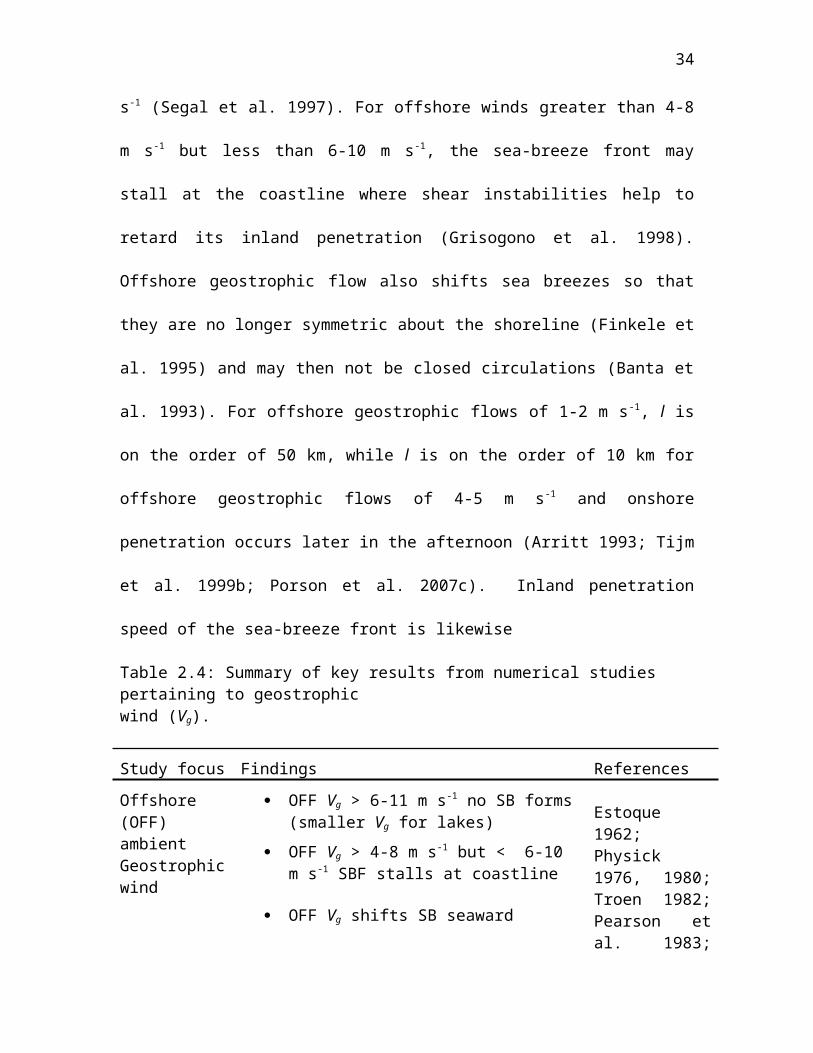
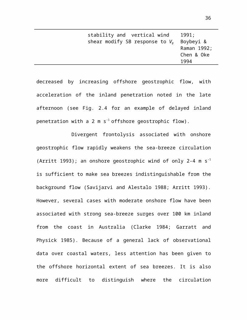
Table 2.4 summarizes the effects of offshore and onshore geostrophic flow on sea
breezes. Most numerical studies with a non-zero background flow have focused on the
impact of offshore geostrophic flow. If the offshore geostrophic wind speed is above
some critical value, then sea breezes do not form as the synoptic pressure gradient
effectively cancels the local pressure gradient. The critical value of the offshore
geostrophic wind above which sea breezes are likely to be absent has been found to be 6-
11 m s-1, depending on the strength of the land-water temperature gradient (Biggs and
Graves 1962; Arritt 1993; Porson et al. 2007c). For small and medium-sized lakes, the
critical value is unknown, but likely ranges between 3-5 m s-1 (Segal et al. 1997). For
offshore winds greater than 4-8 m s-1 but less than 6-10 m s-1, the sea-breeze front may
stall at the coastline where shear instabilities help to retard its inland penetration
(Grisogono et al. 1998). Offshore geostrophic flow also shifts sea breezes so that they
are no longer symmetric about the shoreline (Finkele et al. 1995) and may then not be
closed circulations (Banta et al. 1993). For offshore geostrophic flows of 1-2 m s-1, l is on
the order of 50 km, while l is on the order of 10 km for offshore geostrophic flows of 4-5
m s-1 and onshore penetration occurs later in the afternoon (Arritt 1993; Tijm et al. 1999b;
Porson et al. 2007c). Inland penetration speed of the sea-breeze front is likewise
22
Table 2.4: Summary of key results from numerical studies pertaining to geostrophic wind (Vg).
Study focus Findings References
Offshore (OFF) ambient Geostrophic wind
OFF Vg > 6-11 m s-1 no SB forms (smaller Vg
for lakes)
OFF Vg > 4-8 m s-1 but < 6-10 m s-1 SBF stalls at coastline
OFF Vg shifts SB seaward
SB may lose closed circulation characteristics (no return flow)
l decreases with increasing OFF Vg
OFF Vg delays inland movement of WBF
Magnitude of u, w as perturbations from the mean flow generally increase (decrease) with increasing OFF Vg for Vg less (greater) than 4-6 m s-1
Relationship between OFF Vg and h unclear, although in many cases increases in OFF Vg result in decreases in h
Estoque 1962; Physick1976, 1980; Troen 1982; Pearson et al. 1983; Savijarvi and Alestalo 1988; Arritt 1989, 1993; Bechtold et al. 1991; Yang 1991; Zhong and Tackle 1993; Savijarvi 1997; Finkele 1998; Tijm et al. 1999b; Gilliam et al. 2004; Porson et al. 2007c
Onshore (ON) ambient Geostrophic wind
ON Vg > 3-5 m s-1 no SB forms (or indistinguishable)\
ON Vg shifts SB landward
Magnitude of u, w as perturbations from the mean flow decrease with increasing ON Vg
Magnitude of h generally decreases with increasing ON Vg
Estoque 1962; Esoque & Gross 1981; Troen 1982; Pearson et al. 1983; Clarke 1984; Savijarvi & Alestalo 1988; Arritt 1989, 1993; Zhong & Tackle 1993; Gilliam et al. 2004
Other Peninsula or water body dimensions, atmospheric stability and vertical wind shear modify SB response to Vg
Xian & Pielke, 1991; Boybeyi & Raman 1992; Chen & Oke 1994
23
decreased by increasing offshore geostrophic flow, with acceleration of the inland
penetration noted in the late afternoon (see Fig. 2.4 for an example of delayed inland
penetration with a 2 m s-1 offshore geostrophic flow).
Divergent frontolysis associated with onshore geostrophic flow rapidly weakens the
sea-breeze circulation (Arritt 1993); an onshore geostrophic wind of only 2-4 m s -1 is
sufficient to make sea breezes indistinguishable from the background flow (Savijarvi and
Alestalo 1988; Arritt 1993). However, several cases with moderate onshore flow have
been associated with strong sea-breeze surges over 100 km inland from the coast in
Australia (Clarke 1984; Garratt and Physick 1985). Because of a general lack of
observational data over coastal waters, less attention has been given to the offshore
horizontal extent of sea breezes. It is also more difficult to distinguish where the
circulation terminates over the water due to a lack of a thermal boundary in that region
(Arritt 1989). Finkele (1998) found that the horizontal extension of the circulation over
the water was less sensitive to the offshore geostrophic flow than l, while Arritt (1989)
found that onshore geostrophic flow greatly suppressed the offshore extent of sea breezes
by shifting the entire circulation cell landward.
Most studies agree that w and u in the vicinity of the sea-breeze front are modified
for an offshore ambient geostrophic wind due to convergent frontogenesis (note that u in
these cases refers to the “perturbation” u, which is subtracted from the mean background
flow). Increasing offshore geostrophic flow from 0 to 4-6 m s-1 increases u and w, with a
higher offshore ambient geostrophic wind (greater than 4-6 m s-1) resulting in a slight
weakening of the circulation. The highest w and u for sea breezes associated with
offshore geostrophic winds have been found to occur when frontogenesis is maximized
24
and the inland movement of the sea-breeze front is stalled by the offshore geostrophic
wind (Savijarvi and Alestalo 1988; Bechtold et al. 1991; Arritt 1993). Onshore
geostrophic winds of any speed or offshore geostrophic flow greater than 5-7 m s-1 results
in rapid weakening of u and w (Troen 1982; Arritt 1989, 1993; Bechtold et al. 1991; Xian
and Pielke 1991; Yang 1991).
Sufficiently strong geostrophic winds (> 4 m s-1) act to decrease h through
mechanical turbulence along the upper boundary of the low-level flow. There is no
agreement in the literature on the effect of offshore geostrophic winds less than around 4
m s-1 on h since the mechanical turbulence is offset to varying degrees by frontogenesis
that may locally strengthen and deepen the circulation. Arritt (1993) and Zhong and
Tackle (1993) found that the vertical extent of sea breezes, particularly in the region of
the sea-breeze head, decreases with increasing offshore geostrophic winds while Estoque
(1962) and Troen (1982) found little change in h with increasing geostrophic flow.
Vertical wind shear of the geostrophic wind may also modify sea breezes. Pearson et
al. (1983) indicate that u and the rate of inland movement of the sea-breeze front are
unaffected by vertical wind shear. However, Boybeyi and Raman (1992a) suggest that a
constant vertical wind shear of 2 m s-1 km-1 increases vertical velocities and convergence
near the sea-breeze front, while Chen and Oke (1994) found mechanical mixing of the
low-level sea-breeze flow results from vertical wind shear.
25
Atmospheric Stability (N) and Moisture (q)
The effects of atmospheric stability (N) on sea breezes have been examined primarily
through observational scaling and linear theory. The numerical scaling analyses of Porson
et al. (2007a) and Antonelli and Rotunno (2007) found an inverse relationship between h
and stability (Table 2.2). Many numerical studies, however, only qualitatively discuss
their results for the sea-breeze length scales h and l in terms of Rotunno’s (1983) linear
theory:
l= Nh√ω2− f 2
: latitude<30 ° (2.2)
l =
Nh√ f 2−ω2
latitude≥30 ° (2.3)
where ω represents the diurnal cycle of heating and cooling, f is the Coriolis parameter,
and stability is expressed in terms of the Brunt-Vaisala frequency. However, not
surprisingly, contradictions exist between linear theory and some numerical results.
As shown in Table 2.5, most numerical studies and scaling analyses agree that: (1) a
weakly stably-stratified atmosphere provides a more favorable environment for sea
breezes than does a strongly stably-stratified environment, which acts to “damp” the
circulation and (2) variations in stability affect h and w more strongly than l and u
(Atkinson 1981). Mak and Walsh (1976) show that diurnal differences in stability are the
fundamental reason why nighttime land breezes are weaker than daytime sea breezes.
26
The atmospheric stability specified in approximately 75% of the numerical simulations
reviewed in our study cluster around that of a standard atmosphere (4.0-7.0 K km-1).
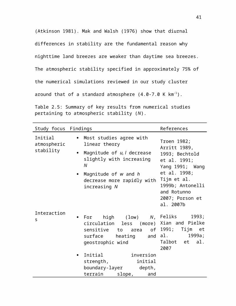
Table 2.5: Summary of key results from numerical studies pertaining to atmospheric stability (N).
Study focus Findings References
Initial atmospheric stability
Most studies agree with linear theory
Magnitude of u, l decrease slightly with increasing N
Magnitude of w and h decrease more rapidly with increasing N
Troen 1982; Arritt 1989, 1993; Bechtold et al. 1991; Yang 1991; Wang et al. 1998; Tijm et al. 1999b; Antonelli and Rotunno 2007; Porson et al. 2007b
Interactions For high (low) N, circulation less
(more) sensitive to area of surface heating and geostrophic wind
Initial inversion strength, initial boundary-layer depth, terrain slope, and multiple inversions also factors
Feliks 1993; Xian and Pielke 1991; Tijm et al. 1999a; Talbot et al. 2007
Only a few studies have investigated the characteristics of sea breezes when the initial
temperature profile deviates substantively from the standard atmosphere (Garratt and
Physick 1985; Yan and Anthes 1987; Savijarvi and Alestalo 1988). Increasing stability
has been found to decrease h (Troen 1982; Arritt 1989, 1993; Xian and Pielke 1991;
Porson et al. 2007a), while a similar dependence has been found between stability and w
(Bechtold et al. 1991; Yang 1991; Arritt 1993; Wang et al. 1998).
Complex interactions among stability and geostrophic winds, terrain height, and
terrain slope are recognized to be important too; for example, Xian and Pielke (1991)
found that for high stability, u becomes insensitive to the size of a heated peninsula,
27
while several authors have noted that decreasing stability increases the dependence of sea
breezes on the geostrophic flow.
According to linear theory (Walsh 1974; Rotunno 1983), u is inversely proportional
to stability while l is proportional to stability, i.e., increasing stability leads to slightly
weaker winds near the shoreline and increased inland extent. In agreement with linear
theory, Yang (1991) found u to decrease slightly with increasing stability. However, there
remains disagreement between studies on the dependence of l on stability. Arritt (1989)
found that increasing stability leads to slight increases in the offshore extent of sea
breezes, while Troen (1982) and Xian and Pielke (1991) found that l decreases slightly
with increasing stability.
The impact of elevated stable layers, multiple stable layers, or near-surface
inversions has also not been systematically analyzed. Tijm et al. (1999a) found that the
strength of the sea-breeze return current and the so-called ‘return-return current’ (caused
by overcompensation of mass by the return current) were a function of the initial
boundary-layer depth and stability. Feliks (1993) found that a sea-breeze circulation
lowered the coastal marine inversion due to subsidence during the day and raised the
inversion at night due to the advection of marine air.
Atmospheric moisture (q) influences sea breezes in a variety of ways, none of which
has been thoroughly explored. Moistening of the shallow sea-breeze flow can occur
rapidly through the surface evaporation of soil moisture (Baker et al. 2001), and the
available low-level moisture in turn modulates the frequency of moist convection along
the sea-breeze front. Convergence between the sea-breeze front and a wide range of other
features leads to convective initiation (Nicholls et al. 1991; Boybeyi and Raman 1992b;
28
Shepherd et al. 2001; Fovell 2005). The effect of the convection itself on the
characteristics of sea breezes has been explored by Song (1986) and Moon (1988); Moon
(1988) found that convective feedbacks strengthened u, w, and h, while Song (1986)
found that deep convection stretches sea breezes vertically. Ambient cloud cover
weakens sea breezes due to the loss of incoming solar radiation (Segal et al. 1986).
Sensitivity Studies of Location-dependent Geophysical Variables
Water Body Dimensions (d) and Shoreline Curvature (r)
Although for sea breezes the water body dimensions can be assumed infinite,
variations in water body dimensions (d) on lake breezes are increasingly important due to
the anthropogenic drying of lake systems such as Lake Chad, the Dead Sea, and the Aral
Sea (Small et al. 2001). Many numerical studies use a circular or 2D slab-symmetric
(i.e., an elongated lake with 2D symmetry) lake such that a single dimension
perpendicular to the shoreline of interest is sufficient (Fig. 2.1). Segal et al. (1997) were
the only investigators to systematically vary lake size; no study has ever systematically
varied water body dimensions in a three-dimensional setting with different water body
dimensions along both axes of a water body. Differences in model set-up and curvature
effects for circular lakes make comparisons difficult between the studies. Water body
dimensions are also an important factor for sea breezes associated with semi-enclosed
bays, which have the added complication of interactions between the bay breeze and the
large-scale sea breeze (Abbs 1986).
Lake breezes associated with large lakes (d > 100 km) have virtually
indistinguishable characteristics from sea breezes (Table 2.6). However, this assumption
may not be true in all circumstances, since Zhu and Atkinson (2004) found that the wider
29
southern Persian Gulf (≈ 400 km) observed stronger gulf breezes than the northern areas
(≈ 250 km).
Table 2.6: Summary of key results from numerical studies pertaining to water body dimensions (d) and shoreline curvature (r).
Study focus Findings References
Medium and large water body dimensions (d> 50 km)
Magnitude of u, w, l and h slowly increase with increasing d for d between 50-100 km
Negligible dependence of SB on d greater than 100 km
Physick 1976; Yan and Anthes 1988; Segal et al. 1997; Boybeyi and Raman 1992a; Savijarvi 1997
Small water body dimensions (d< 50 km)
Magnitude of u, w, l, and h rapidly increase with increasing d
Large shoreline curvature-induced divergence and less available cool air responsible for weaker SB for small d
Physick 1976; Neumann and Mahrer 1975; Yan and Anthes 1988; Zhong et al. 1991; Boybeyi and Raman 1992a; Shen 1998
Curvature Convex shoreline strengthens SB
Concave shoreline weakens SB
Mahrer and Segal 1985; McPherson 1970; Arritt 1989; Gilliam et al. 2004; Boybeyi and Raman 1992a
For medium (d ≈ 50-100 km) and small (d ≈ 5-50 km) water bodies, the
characteristics and intensity of sea breezes vary nonlinearly due in part to shoreline
curvature effects (Boybeyi and Raman 1992a). The overlying boundary layer over a
small lake or gulf is subject to greater influence from the ambient land boundary layer in
addition to the two mirror circulations competing for limited cool, low-level air. As the
size of a water body decreases, the associated circulations become less well-developed,
30
i.e., smaller u and w, shallower h, with less inland penetration and weaker fronts (Table
2.6). The relative increases in u and w for increases in lake dimensions between 5 and 50
km are significantly larger than the increases associated with further increases in water
body dimensions between 50 and 100 km (Neumann and Mahrer 1975; Physick 1976;
Boybeyi and Raman 1992a; Segal et al. 1997). In contrast, offshore subsidence may
increase with decreasing water body dimensions due to enhanced convergence between
the two mirror circulations (Physick 1976; Sun et al. 1997). Little is known about the
dependence of h and l on the magnitude of the water body dimensions except that smaller
water body dimensions tend to lead to smaller h and l (Physick 1976; Zhong et al. 1991).
The frequency of occurrence of sea breezes diminishes as water body dimensions
decrease, since smaller-scale circulations are more easily destroyed by the prevailing
background geostrophic flow. While the magnitude of the geostrophic wind needed to
destroy sea breezes for given water body dimensions has not been studied in detail, Shen
(1998) found that a lake breeze failed to form for a 5 km lake with a geostrophic wind of
4 m s-1.
Spatial heterogeneities in the land-surface sensible heat flux associated with islands
or strips of land with different soil moisture or vegetation type resulting in “inland
breezes” are also applicable to understanding sea breezes for small water body
dimensions (Ookouchi et al. 1984; Segal et al. 1988; Mahrt et al. 1994; Courault et al.
2007). The intensity of inland breeze circulations caused by the difference in land-surface
sensible heat fluxes between two land-surface types is typically weaker than a sea breeze,
in part due to the enhanced turbulent mixing on the ‘moist’ land side compared to the
negligible thermal plumes noted over water (Yan and Anthes 1988; Segal and Arritt
31
1992). Small water bodies likely have boundary layers that are a hybrid between large-
scale sea breezes and moist land situations.
Shoreline curvature (r) can strongly affect interactions between the prevailing winds
and sea breezes. A convex coastline (coastline bulging out from the land) yields
convergence of the onshore low-level flow and strengthens the circulation, while a
concave coastline (coastline bulging in from the ocean) weakens the circulation through
divergence (McPherson 1970; Arritt 1989; Gilliam et al. 2004). The impact of the
curvature associated with large and small circular lakes has been examined, with smaller
lakes yielding more divergent circulations (Boybeyi and Raman 1992a). Baker et al.
(2001) noted that shoreline curvature had a major impact on the location and timing of
sea-breeze initiated precipitation.
Terrain Height (ht) and Slope (s)
Most numerical studies examining the influence of topography on sea breezes were
focused on understanding local terrain effects on sea breezes and did not systematically
vary the slope or height of the terrain (Table 2.7). Topography can enhance sea breezes
through elevated heating and cooling, which drives slope flows that combine with sea
breezes, or suppress them by mechanically blocking the onshore flow (Atkinson 1981;
Abbs and Physick 1992). The dependence of sea breezes on terrain is controlled by the
terrain slope (s), length of the terrain slope, terrain height (ht), location of the mountain
relative to the coastline, and atmospheric stability. Although no study has looked
systematically at the effects of terrain height on sea breezes, Porson et al. (2007b) were
the first to systematically vary both atmospheric stability, slope angle, and slope length.
32
They found that l and h are highly dependent on both terrain slope and atmospheric
stability.
Table 2.7: Summary of key results from numerical studies pertaining to terrain slope (s) and terrain height (ht).
Study focus Findings References
Terrain slope/Terrain height
Slope of sufficiently low steepness: thermally-driven slope flows combine with SB to enhance u, w, l and h
Combined slope and SB may lead to earlier SBF passage
Slope of sufficiently high steepness: inland penetration of SBF is suppressed and u, w, l and h decrease
Distance between shoreline and mountain, absolute height of mountain,length of slope, H, and N are key factors in determining critical slope angle
Mahrer & Pielke 1977; Asai & Mitsumoto 1978; Ookouchi et al. 1978; Estoque & Gross 1981; Kikuchi et al. 1981; Segal et al. 1983; Neumann & Savijarvi 1986; Ramis & Romero 1995; Miao et al. 2003; Porson et al. 2007b;
Other Channeling of SB may locally
enhance u, w, and l Small mountains inland from coast
can block inland penetration Mountain slope can produce “chimney
effect” stalling SBF
Ookouchi et al. 1978; Segal et al. 1983; Neumann & Savijarvi 1986; Lu and Turco 1994; Ramis & Romero 1995; Millan et al. 2000; Darby et al. 2002
Most numerical sea-breeze studies concerning terrain slope have focused on u, w,
and l (Table 2.7). These studies have found that on a heated slope of sufficiently low
steepness (less than 2.29° according to Asai and Mitsumoto (1978) or ≈0.8° according to
33
Porson et al. (2007b)), thermally-driven slope flows may couple with sea breezes and
increase u, w, l, and h (Mahrer and Pielke 1977; Estoque and Gross 1981; Miao et al.
2003). Combined sea-breeze and slope flows may also lead to an earlier inland sea-breeze
front passage (Ookouchi et al. 1978; Kikuchi et al. 1981). A slope of sufficiently high
steepness will act to block the inland penetration of the sea-breeze front and decrease u,
w, l, and h (Asai and Mitsumoto 1978; Segal et al. 1983; Neumann and Savijarvi 1986;
Porson et al. 2007b). The critical slope angle at which the coupling of thermally-driven
slope flows outweighs the terrain blocking effects is variable and depends on the vertical
stability profile, magnitude of slope heating (e.g., vegetation type, aspect), the total length
of the slope, the distance from the coastline to the mountain, and the absolute height of
the mountain. A secondary effect of topography on sea breezes is channeling, which can
locally enhance u, w, and l (Abbs 1986; Abbs and Physick 1992; Segal et al. 1997).
Darby et al. (2002) found that l may occur on multiple scales depending on terrain
height and distance inland of a mountain range. Miao et al. (2003) determined that l was
similar between “terrain” and “no terrain” simulations while h was enhanced. Asai and
Mitsumoto (1978) and Lu and Turco (1994) suggest that upslope flows associated with
topography located inland away from the coast do not readily couple with sea breezes
compared to upslope flows associated with topography near the coast. However, even
small mountains located some distance inland can act to block the late-afternoon inland
acceleration of the sea-breeze front or remove its low-level baroclinicity (Ookouchi et al.
1978).
Lu and Turco (1994) and Millan et al. (2000) discuss topographic effects on pollutant
transport, including the so-called ‘chimney effect’ where coastal mountains stall the
34
inland penetration of the sea-breeze front and set up a quasi-stationary region of upward
vertical motion near the mountain crest. The coupling of sea breezes with slope flows in
complex terrain makes the simple circulation cell illustrated in Fig. 2.2 inaccurate (Millan
et al. 2000). Banta et al. (1993) observed sea breezes in complex terrain that did not have
a return flow and hypothesized that slope flows provided the mass compensation
normally provided by the return flow, although Miao et al. (2003) found that the presence
of sloping terrain actually enhanced the magnitude of the return flow.
Coriolis Parameter (f)
Numerical studies of sea breezes have generally been conducted at fixed latitudes;
consequently, knowledge of the effects of variations in latitude on sea breezes have been
largely limited to observational comparisons and linear or scale analysis (e.g., Neumann
1977; Rotunno 1983). The Coriolis force, typically specified by the magnitude of the
Coriolis parameter (f), influences the wind direction and l, u, and h of sea breezes.
The Coriolis force rotates the sea breeze 360° over a 24-hr inertial period (Haurwitz
1947). Coriolis effects are small for most of the daytime life cycle of sea breezes when
friction and surface heating dominate (Yan and Anthes 1987). However, after about 6
hours from onset, sea breezes begin to rotate into a plane parallel to the coast and weaken
due to the Coriolis force (Anthes 1978; Yan and Anthes 1987; Xian and Pielke 1991).
The numerical scaling analyses of Tijm et al. (1999b) and Antonelli and Rotunno (2007)
give further evidence on the increasing importance of f during the latter stages of the sea-
breeze life cycle (Table 2.2). The magnitude of u and surface friction modulate the
influence of the Coriolis parameter for a given latitude. The Coriolis force may also
35
interact with w and shoreline shape to determine areas of breeze-induced convergence
(Boybeyi and Raman 1992a).
The Coriolis force primarily affects l and u. Yan and Anthes (1987) studied the
effects of variations in the Coriolis parameter at latitudes of 20°, 30°, and 45° N and
found results consistent with the linear analysis of Rotunno (1983) (Eq. 2.2). In the
absence of friction, l was less (more) than 100 km and in (out of) phase with the diurnal
heating poleward (equatorward) of 30° latitude. They hypothesized that land breezes at
high latitudes may result more from the rotation of sea breezes by the Coriolis force than
the reversing diurnal pressure gradient. For locations in a high land-surface sensible heat
flux, low latitude environment, the small Coriolis force may still be critical. Garratt and
Physick (1985) found sea breezes at 15° S latitude had inertial periods of approximately
46 hours, allowing for very slow turning of the winds and the extreme l observed in
Australia.
Surface Roughness Length (zo)
Frictional drag acts to destroy the developing horizontal pressure gradient associated
with sea breezes (Anthes 1978). Frictional effects are induced by both surface roughness
and turbulent motions (e.g., convection and Kelvin-Helmholtz instability), and while the
aerodynamic roughness length (zo) has a large influence on the developing circulation, the
dependence of SB on observed ranges of roughness length associated with different land
types and land-water surface contrasts is generally small (Neumann and Mahrer 1975;
Savijarvi and Alestalo 1988; Arritt 1989; Yang 1991; Boybeyi and Raman 1992a; Tijm et
al. 1999b). Spatial perturbations in the roughness length (these perturbations in most
modeling studies occur at length scales that cannot be resolved, i.e., sub-grid scale
36
variability) have also been found to have little effect in ensemble-mean sea-breeze
statistics (Garratt et al. 1990). Numerical investigations of sea breezes for the most part
specify constant roughness lengths over land and water surfaces. Specified surface
roughness lengths for the studies listed in Table 1 range between 0.04-0.05 m over land
and 0-0.2 mm over water. However, more recent numerical modeling by Courault et al.
(2007) and linear scaling by Drobinski and Dubos (2009) show that the roughness length
helps to control h for small inland-breeze type circulations. Boybeyi and Raman (1992a)
found that increasing roughness length resulted in an enhanced circulation with a larger
vertical transfer of heat, while Kala et al. (2010) found that decreasing roughness length
resulted in higher surface winds and increased surface moisture advection. Surface
friction also influences the formation of clef and lobe instability caused by horizontal
convective rolls (Dailey and Fovell 1999).
Discussion
Modeling Limitations and Comparison with Observations
The majority of numerical studies concerning sea breezes were conducted using two-
dimensional, hydrostatic models. The differences between hydrostatic versus non-
hydrostatic simulations are typically small when the model horizontal grid spacing is
larger than 1 km (Avissar et al. 1990), and because nonhydrostatic effects act to weaken
mature SB, hydrostatic models may overestimate sea-breeze intensity (Martin and Pielke
1983). The modeled vertical velocities and frontal structure in most hydrostatic
simulations are understandably poor (Avissar et al. 1990). Although the use of three-
dimensional models is important to realistically simulate planetary boundary-layer (PBL)
turbulence and the interactions between horizontal convective rolls and other small-scale
37
PBL features associated with sea breezes, two-dimensional models are adequate for many
idealized simulations.
Many numerical simulations of sea breezes have been conducted with horizontal grid
spacing greater than 2 km in combination with lower-order PBL turbulence
parameterizations (Table 2.1). Inadequate treatment of PBL turbulence may be the largest
deficiency of many early numerical models of sea breezes (Briere 1987; Yang 1991), and
may be the reason that most numerical simulations are unable to reproduce the observed
afternoon slowing of the sea-breeze front associated with turbulent frontolysis (Simpson
et al. 1977). Increasing the horizontal resolution of numerical simulations or using more
sophisticated PBL parameterization schemes does not always yield improved results, as
the increase in resolution may be insufficient to significantly improve the resolved
turbulence in the PBL (Colby 2004; Novak and Colle 2006; Srinivas et al. 2007).
It is beyond the scope of this review to conduct a thorough comparison between
numerical and observational results. On average, model estimates of u, l, and h differed
from observations by around 25% for those studies listed in Table 2.1 and for which it is
possible to make such comparisons. The basic structures of sea breezes are well-
represented in most cases, but the fine-scale features and interactions between the sea
breeze and the geophysical variables are generally not captured. Consequently, it is not
surprising that most numerical simulations were deficient in predicting the frontal
intensity, l, and w.
Comparing numerical experiments in which only a single variable is perturbed to the
constantly evolving atmosphere is difficult. Despite this constraint, applying scaling laws
to observational datasets has provided the most comprehensive observational evidence of

38
the effects of geophysical variables on sea breezes. The observational scaling analyses by
Steyn (1998, 2003) and Kruit et al. (2004) investigate the effects of the land surface
sensible heat flux, atmospheric stability, and Coriolis parameter on sea breezes. Their
results generally agree with the numerical scaling by Porson et al. (2007a) and Antonelli
and Rotunno (2007) (Table 2.2), with some differences possibly attributable to the unique
local characteristics of the observational datasets used. A general increase in the
characteristic sea-breeze speed and length scales is noted in dry areas or low latitudes that
typically observe high daytime surface-sensible heat fluxes compared to regions that
observe low daytime surface-sensible heat fluxes (Atkinson 1981; Kruit et al. 2004).
Observational studies also reinforce the numerical findings of the effects of the ambient
geostrophic wind on sea breezes. A decrease in l and h and an increase in w and
temperature gradient across the sea-breeze front have all been observed for the case of
moderate offshore wind (Simpson et al. 1977; Zhong and Tackle 1993; Atkins et al.
1995; Helmis et al. 1995; Melas et al. 1998; Asimakopoulos et al. 1999; Chiba et al.
1999). Observations of sea breezes near lakes of different sizes also corroborate the
numerical findings that generally weaker sea breezes occur with smaller lake dimensions
(Bitan 1977; Atkinson 1981; Segal et al. 1997; Sun et al. 1997; Samuelsson and
Tjernstrom 2001). Observations have shown the continuation of tropical sea breezes at
night due to a lack of turning of the wind by the Coriolis force. The coupling of slope and
sea-breeze circulations has also been observed (Atkinson 1981; Abbs 1986; Banta et al.
1993; Mastrantonio et al. 1994).
Recent High-Resolution Studies
39
Since 1990, a number of two- and three-dimensional idealized numerical studies
have been made at a horizontal grid spacing of approximately 100 m, where most
boundary-layer turbulence is explicitly resolved (e.g, Hadfield et al. 1991, 1992; Sha et
al. 1991, 1993, 2004; Fovell and Daily 2001; Letzel and Raasch 2003; Antonelli and
Rotunno 2007; Cunningham 2007; Talbot et al. 2007). These large-eddy simulations
(LES) provide insight into the fine-scale structure of sea breezes and interactions between
sea breezes and boundary-layer features, such as lobe and cleft instabilities and horizontal
convective rolls (Fig. 2.5). Observational studies have corroborated the horizontally non-
uniform structure and oscillatory propagation speed of the sea-breeze front simulated by
models run at high resolution (Yoshikado 1990; Wakimoto and Atkins 1994; Wood et al.
1999; Stephan et al. 1999; Puygrenier et al. 2005). A number of air pollution dispersion
models have simulated the ‘translocation’ or significant vertical advection of pollutants
by narrow frontal plumes, the effect of the internal boundary layer associated with sea
breezes on pollutant fumigation, interactions between urban-induced circulations and sea
breezes, and the effects of turbulence and multilayer stratification on recirculation
(Lemonsu et al. 2006; Thompson et al. 2007).
A number of recent studies have investigated the interactions between horizontal
convective rolls and the sea-breeze front. Daily and Fovell (1999) found that the sea-
breeze front developed considerable three-dimensional variability in the presence of
horizontal convective rolls oriented perpendicular to the sea-breeze front, while frontal
uplift and propagation speed were influenced by interactions with horizontal convective
rolls oriented parallel to the sea-breeze front. Weak lift associated with sea breezes was
found to be important for convective initiation by Fovell (2005). Kelvin-Helmholtz
40
instability billows are also another important fine-scale feature behind the sea-breeze
front that may trigger or enhance convection, redistribute pollutants, and induce a top-
friction force that slows the sea-breeze front’s inland progression (Rao et al. 1999; Rao
and Fuelberg 2000; Plant and Keith 2007). Ogawa et al. (2003) modeled episodic
strengthening and weakening of the sea-breeze front associated with Rayleigh-Bernard
convection. With the exception of Antonelli and Rotunno (2007), numerical constraints
41
Figure 2.5. Recent topics of interest in high-resolution numerical modelling studies of SB including: horizontal convective roll (HCR), convective boundary layer (CBL), Kelvin-Helmholtz instability (KHI), and the thermal internal boundary layer (TIBL).
42
have prevented LES studies from investigating the dependence of sea breezes on the
various geophysical variables. Thus, as computational capabilities improve, there is a
need to revisit many of the earlier numerical sensitivity studies at LES resolution.
The Dependence of Sea Breezes on Geophysical Variables
All ten geophysical variables listed in this study affect the characteristics of sea
breezes. The fundamental driver of sea breezes is the differential sensible heating
between the land and water surfaces, and variations in land-surface sensible heat flux,
background geostrophic wind, and atmospheric stability have a pronounced effect on the
intensity of sea breezes at a given location, while water body dimensions, Coriolis force,
terrain height, and terrain slope may explain differences in sea breezes around the world.
The impacts of shoreline curvature, roughness length, and atmospheric moisture on sea
breezes are generally smaller.
As a way to assess the relative impacts of these variables, we summarize in Table 2.8
the fractional change (i.e., change divided by original value) in the length and velocity
scales of sea breezes to 100% increases in the magnitudes of the geophysical variables. In
general, most studies agree on the sign of the observed sensitivity of sea breezes to
variations in a given geophysical variable. However, the magnitude of that dependence
can vary widely between studies.
Of the ten geophysical variables, the effects of variations in land-surface sensible
heat flux and geostrophic wind on sea-breeze speed and length scales are the most widely
studied and quantified (Table 2.8). All studies agree that higher values of land-surface
sensible heat flux are associated with stronger, deeper sea breezes. There is poor
43
Table 2.8: The impact of a 100% increase in the geophysical variables on the mid-afternoon sea-breeze length and velocity scales expressed as the fractional change (change divided by original value). Arrow () denotes a specific doubling of a geophysical variable.
100% increase in
% change umax
% change wmax
% change
lmax
% change
h
Reference
Temporally-dependent geophysical variables
H -- -- 15-100 -- Physick 1980; Tijm et al. 1999b30 25 25 -- Troen 198264 80 -- -- Shen 199880 200 30 30 Miao et al. 2003
30-40 -- 40 35 Antonelli & Rotunno 2007; Porson et al. 2007a
Vg : 1 2 m s-1 offshore
10 25 -50 -5 Arritt 1993
-- -- -15 -- Savijarvi and Alestalo 1998-- -- -40 -- Tijm et al. 1999b
Vg : 3 6 m s-1 offshore
-5 -10 -- -50 Arritt 1993
-- -- -125 -- Porson et al. 2007c-- -- -100 -- Savijari and Alestalo 1998
Vg: 1 2 m s-1
onshore-25 -25 -- -- Arritt 1993
N -10 -10 -5 -75 Troen 1982-15 -- 0 -40 Arritt 1989-25 -50 -- -- Yang 1991-- -- -- -100 Antonelli and Rotunno 2007; Porson et al.
2007aLocation-dependent geophysical variables
d: 10 20 km
75 -- -- -- Segal et al. 1997
d: 25 50 km
25-35 100 -- -- Segal et al. 1997; Neumann and Mahrer 1975; Boybeyi and Raman 1992
d : 50 100 km
10-20 100 -- -- Segal et al. 1997; Physick 1976
f: 0° 20° 40 -- 25 -- Yan and Anthes 1987f: 20° 45° 100 -- 200 -- Yan and Anthes 1987f: 20° 45° 5 100 -- -- Yang 1991
zo 0 -- 0 -- Savijarvi and Alestalo 1988; Tijm et al. 1999b
1 5 -- -- Yang 1991
s: No slope slope
100 200 Asai and Mitsumoto 1978; Kikuchi et al. 1978
44
15 200 0 20 Miao et al. 2003
agreement outside of the scaling studies (Table 2.2) as to the magnitude of the effects of
variations in the land-surface sensible heat flux on u and w. Despite the fact that
simulations with a horizontal grid spacing greater than 1 km do not fully resolve vertical
motions associated with the sea-breeze front, w is very sensitive in some studies to
variations in land-surface sensible heat flux, presumably due to changes in convective
thermals near the sea-breeze front. There is better agreement that l and h both increase by
around 25-50% for a 100% increase in the land-surface sensible heat flux.
The magnitude of the geostrophic wind modulates l and h. The presence of an
offshore geostrophic wind of 2 m s-1 (Fig. 2.4) delays the onshore arrival of the sea-
breeze front by up to several hours and l by up to 50% (Physick 1980; Tijm et al. 1999b).
Variations in the magnitude of the offshore geostrophic wind affect l more strongly than
u, w, and h in most studies (Table 2.8). Increasing offshore geostrophic winds from 1 to 2
m s-1 results in a 10-25% increase in u and w associated with convergent frontogenesis,
while further increase in the offshore geostrophic winds from 3 to 6 m s-1 results in a 5-10
% decrease in the magnitude of u and w, and doubling the offshore geostrophic wind
from 3 to 6 m s-1 greatly reduces the extent of inland penetration.
Stability, besides indirectly modulating the effects of topography, geostrophic wind,
and other geophysical variables, has its largest impact on the vertical scale of the
circulation, with a 100% increase in stability resulting in a 40-100% decrease in h and a
10-50% decrease in w. The modeling results reveal only slight decreases in u and l
associated with a doubling of stability, providing some evidence that linear theory may
overestimate the impacts of changes in stability on l.
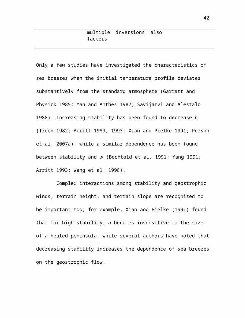
45
There are only a handful of studies that quantify the effects of water body dimensions
on sea breezes, and these only discuss the speed scales. Increasing the dimensions of a
water body from 25 to 50 km yields roughly a 30% increase in u, while increasing the
water body dimensions further from 50 to 100 km only results in another ≈15% increase
in u. Although w is quite sensitive to changes in water body dimensions—a 100%
increase in water body dimensions results in a doubling of vertical velocities—it is
unclear why changes in w do not decrease for larger lakes sizes in a similar fashion as for
u.
The effect of the Coriolis force on late afternoon sea-breeze strength is significant
(Coriolis effects are minimal through the early afternoon hours), and increases with
increasing latitude (Yan and Anthes 1987). Terrain slope forcing on sea breezes is
difficult to compare since each study used unique combinations of terrain height and
slope. Simulations with mountains yield small (15-20%) to large (100-200%) increases in
the magnitude of u, w, h, and l compared to when they are removed.
Gaps in Understanding and Recommendations for Future Research
Despite the extensive number of scientific studies devoted to understanding the
influence of geophysical parameters on sea breezes, gaps remain, and are largely due to
numerical and computational limitations such that a limited range of parameter values
have been examined. For example, most studies used values of land-surface sensible heat
flux typical of those observed during midlatitude summer. Testing the interdependence
and interactions that may exist between the geophysical variables has generally not been
feasible. Horizontal grid spacing greater than 2 km used in most numerical simulations
has limited the realism of the vertical motion field and a wide array of boundary-layer
46
interactions. An extended analysis of the evolution of sea breezes in the context of both
time of day and the temporal evolution of the geophysical variables (i.e., sensible heat
flux or background winds) is needed. The geophysical variables are clearly not
temporally invariant as many numerical studies have chosen to assume. Further work on
the dependence of sea breezes on sets of basic configurations of water body dimensions,
the area of heated land surface, coastline geometry, and surrounding topography is
warranted. A better understanding of the effects of the geophysical variables on the sea-
breeze speed and depth scales inland from the coastline is also needed. For example,
Garratt and Physick (1985) found that the depth of the sea-breeze gravity current inland
from the Australian coast varied between 550 and 1650 m during the expansion and
contraction of the convective boundary layer.
In addition to these larger concerns, there are a number of specific research questions
that remain unanswered and are briefly mentioned here. Despite the widespread
occurrence of stable layers in the marine boundary layer, most numerical studies used
idealized standard atmospheric temperature profiles. Hence, incorporating realistic
vertical stability profiles and examining further the interactions between stability and the
other geophysical variables is quite important. Initiation of sea breezes remains a topic
for further investigation since three different possible explanations for the formation of
sea-breeze pressure gradients are presented by Tijm and Van Delden (1999). Given that
hodograph rotation has been largely neglected since the early study of Haurwitz (1947),
simulating the hodograph rotation under a wide array of geophysical variables is a topic
for future exploration. Steyn and Kallos (1992) found that anticlockwise rotation of the
sea-breeze hodograph occurred (opposite the typical Coriolis-induced clockwise rotation)
47
due to terrain effects. Improved understanding of how geophysical variables influence
vertical velocities and the fine-scale structure and propagation of the sea-breeze front is
needed now that numerical simulations are able to accurately simulate the fine-scale
frontal structure. Very little research has been conducted on the effects of the geophysical
variables on the return current or the return-return current. As discussed by Tijm et al.
1999, the ‘return-return’ current is a secondary flow above and in the opposite direction
as the primary sea-breeze return current which exists to balance out an over-
compensation in the mass flow by the return flow. Other topics for future research
include over-water subsidence for sea and lake breezes and convective initiation. Finally,
the presence of a sea-breeze ‘precursor’ noted in some observational studies (Banta et al.
1993; Mastrantonio et al. 1994) has not been numerically simulated to our knowledge.
The results of this survey point out a number of areas where future research could
benefit pollutant transport studies. Reducing the surface concentration of pollutants
trapped within sea breezes is most readily accomplished by increasing ventilation.
Further research on the impacts of changes in the geophysical variables on the horizontal
speed and vertical depth scales of sea breezes and the subsequent rates of ventilation and
recirculation are needed. The importance of sea-breeze frontogenesis and interactions
between sea breezes and a host of boundary-layer features (e.g., Kelvin-Helmholtz
instability and horizontal convective rolls) in transporting and removing pollutants from
the sea-breeze circulation also remains an active area of interest.
As discussed by Shaw et al. (2009), wind power resources in coastal regions are
dependent on the magnitude of the sea-breeze flow. A topic for further study concerns the
upper limit to wind speeds in high sensible heat flux environments as a result of turbulent
48
frontolysis. Analysis of the wind resource offshore over open water under a wide range of
the geophysical variables is needed. For example, the shifting of the sea-breeze
circulation by the geostrophic flow may enhance the low-level winds in the immediate
offshore zone. Surface roughness effects also need to be revisited under a wide array of
atmospheric conditions; Garvine and Kempton (2008) found that wind speeds at hub
height were three times higher over the open shelf waters than along the shore.
CHAPTER 3
LARGE-EDDY SIMULATION OF A SEA BREEZE
Motivation and Background
Numerical limitations have constrained most previous numerical studies of lake and
sea breezes to two-dimensional hydrostatic models run at coarser than 2 km horizontal
resolution. These models have been unable to adequately resolve three-dimensional
boundary-layer turbulence or updrafts in the vicinity of the sea-breeze front (Chapter 2).
These studies also generally focused on the mature afternoon sea-breeze characteristics
and structure rather than the entire daytime sea-breeze life cycle and were limited in the
range of forcing of the geophysical variables being investigated. In addition, lake breezes
for small lakes, which are notably different than sea breezes, have not been rigorously
studied numerically or observationally.
The ability of large-eddy simulations (LES) to simulate sea breezes with greater
realism than coarse-resolution models has been amply demonstrated (Sha et al. 1991,
1993, 2004; Dailey and Fovell 1999; Rao et al. 1999; Fovell and Dailey 2001; Ogawa et
al. 2003; Fovell 2005). However, these studies were more concerned with simulating
detailed structures and interactions between a single sea-breeze life cycle and other
boundary-layer phenomena (e.g., horizontal convective rolls, Kelvin-Helmholtz
instabilities) than ascertaining the sensitivity of these circulations to variations in
geophysical variables. Most recently, Antonelli and Rotunno (2007) conducted LES on
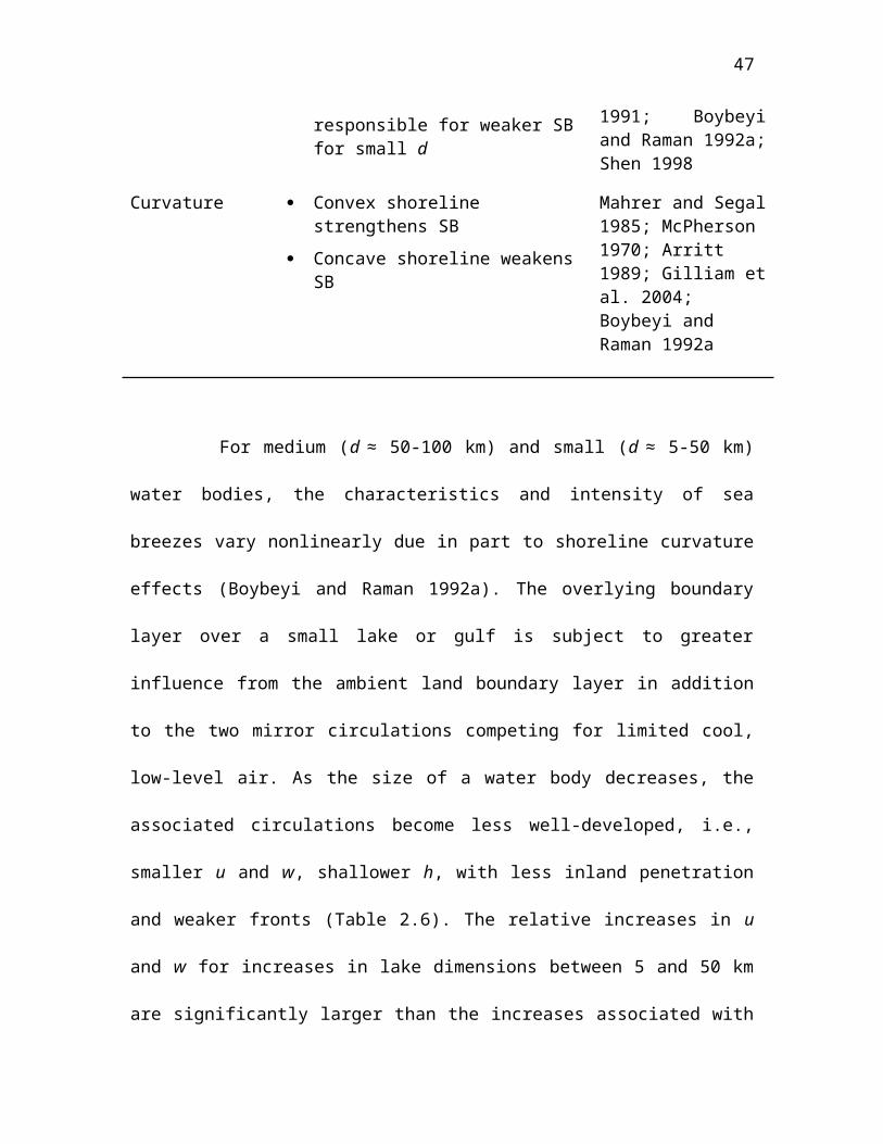
50
the effects of variations in several geophysical variables on the onset of a sea breeze. In
this study, we expand on the work of Antonelli and Rotunno (2007) and increase the
simulation duration and spatial extent, as well as include a diurnally-varying land-surface
sensible heat flux (instead of their fixed land-surface sensible heat flux), and consider the
effects of water body diameter and ambient geostrophic flow.
The goal of this study is to determine the sensitivity of daytime lake and sea-breeze
circulations to several key geophysical variables using LES. Specifically, we aim to
provide new insight into the temporal and spatial evolution of sea and lake breezes in
terms of these variables, and to improve our general understanding of lake breezes for
small- and medium-sized lakes. This study investigates variations in four geophysical
variables that generally have the largest impact on lake and sea breezes: the land-surface
sensible heat flux, initial atmospheric stability, opposing background wind speed, and
water body dimension. As can be expected, a number of large-eddy simulations are
needed to determine the effects of variations in and interactions among these geophysical
variables on daytime sea- and lake-breeze evolution. Other geophysical variables (e.g.,
Coriolis force, topography, shoreline curvature) will not be discussed.
As discussed in Chapter 2, the cross-coast horizontal wind component u and the
horizontal inland extent l of sea and lake breezes are the two most commonly used
measures of sea-breeze intensity. We define u as the low-level (~30 m above ground) sea
breeze flow measured at the coast (for positive values of u, the sea-breeze flow is directed
onshore), and l will be defined as the distance inland (at any given time) of the sea- or
lake-breeze front, defined using the furthest inland location of a non-zero horizontal
onshore flow (averaged along the y-axis). A well-defined thermodynamic boundary does
51
not exist in some simulations and is therefore not used to define the inland location of the
sea breeze. In several cases we will also refer to the depth h of the low-level onshore flow
at the coast. Focusing on these simple measures of sea- and lake- breeze intensity
provides a means to initially evaluate the roughly 75 gigabytes of model output generated
by each simulation. Intercomparison between the LES and previous coarse-resolution
numerical studies and observational scaling analyses requires focusing on these
historically-used measures. A plethora of information regarding lake and sea-breeze
spatiotemporal structure is inherent in the LES and obviously cannot be gleaned from a
simple analysis of u, l, and h. More sophisticated analysis methods will follow in the
future.
Weather and Forecasting Model as a Large-Eddy Simulation
The Weather Research and Forecasting (WRF) model is the first fully-compressible,
nonhydrostatic atmospheric model suitable for both weather prediction and research over
a wide range of scales (Skamarock and Klemp 2008). Additional details on the WRF
model numerics, dynamics, and physics can be found in Skamarock et al. (2008). The
WRF is beginning to be used extensively for LES to examine boundary-layer flow
(Cunningham 2000; Moeng et al. 2007; Rotunno et al. 2009; Catalano and Moeng 2010;
Mirocha et al. 2010; Lundquist et al. 2010). For this study we used the WRF model
(version 3.2) at high enough horizontal resolution (~100 m) that no planetary boundary
layer (PBL) parameterization is required. A summary of WRF model characteristics is
given in Table 3.1. The WRF model uses a terrain-following hydrostatic-pressure
52
Table 3.1:WRF model dynamics and physics options.
Model parameterSelection (wrf namelist options
in italics)
Vertical gridTerrain-following hydrostatic-
pressure
Horizontal grid Arakawa C-grid
Numerical core Nonhydrostatic
Time integration Runge-Kutta 3rd order time-
splitting
Horizontal momentum 5th order advection
Vertical momentum 3rd order advection
Mixing Physical space (stress form) (diff_opt = 2)
Surface layer schemeMonin-Obukhov
(sf_sfclay_physics = 1)
Radiation scheme None
PBL scheme None
Land surface model None
Subgrid-scale turbulence
1.5 order TKE (km_opt = 2)
with NBA of Mirocha et al. 2010
(sfs_opt = 2)
Knievel et al. 2007
53
coordinate, Arakawa C-grid staggering, and a time-splitting scheme to run acoustic and
gravity wave modes with a very small time step. The model was configured with a 3rd
order Runge-Kutta time integration scheme and a 5th order spatial discretization scheme.
A dry atmosphere was considered and surface fluxes were prescribed so no radiation,
microphysical, PBL, or land-surface parameterizations were needed. Surface drag was
computed using standard Monin-Obuhkov similarity theory. While most of the turbulent
eddies are explicity represented in LES, small-scale turbulence below the numerical grid
size must be parameterized using a subgrid-scale scale model. The standard WRF
subgrid-scale models are the turbulent kinetic energy (TKE) model (1.5-order prognostic
TKE closure) and the Smagorinsky 1st order closure (3D). Fortunately, the Nonlinear
Backscatter Anisotropic (NBA) model of Mirocha et al. (2010) was implemented into
WRF in version 3.2 which uses the subgrid TKE predicted by the standard WRF 1.5-
order prognostic TKE model but adds 2nd order terms to account for backscatter and
anisotropic effects (under certain conditions, these terms may be significant, e.g,
backscatter may be important in regions of high wind shear or high stability, while
anisotropic effects may be important in regions of high instability). The WRF model also
contains no explicit low-pass filter but rather implicitly provides the filtering that
separates the resolved and subfilter components using the numerical grid. This is another
source of error that has been corrected for by Mirocha at al. (2010) using a Resolvable
Subfilter-scale Stresses (RSFS) model. The RSFS model has not yet been included as part
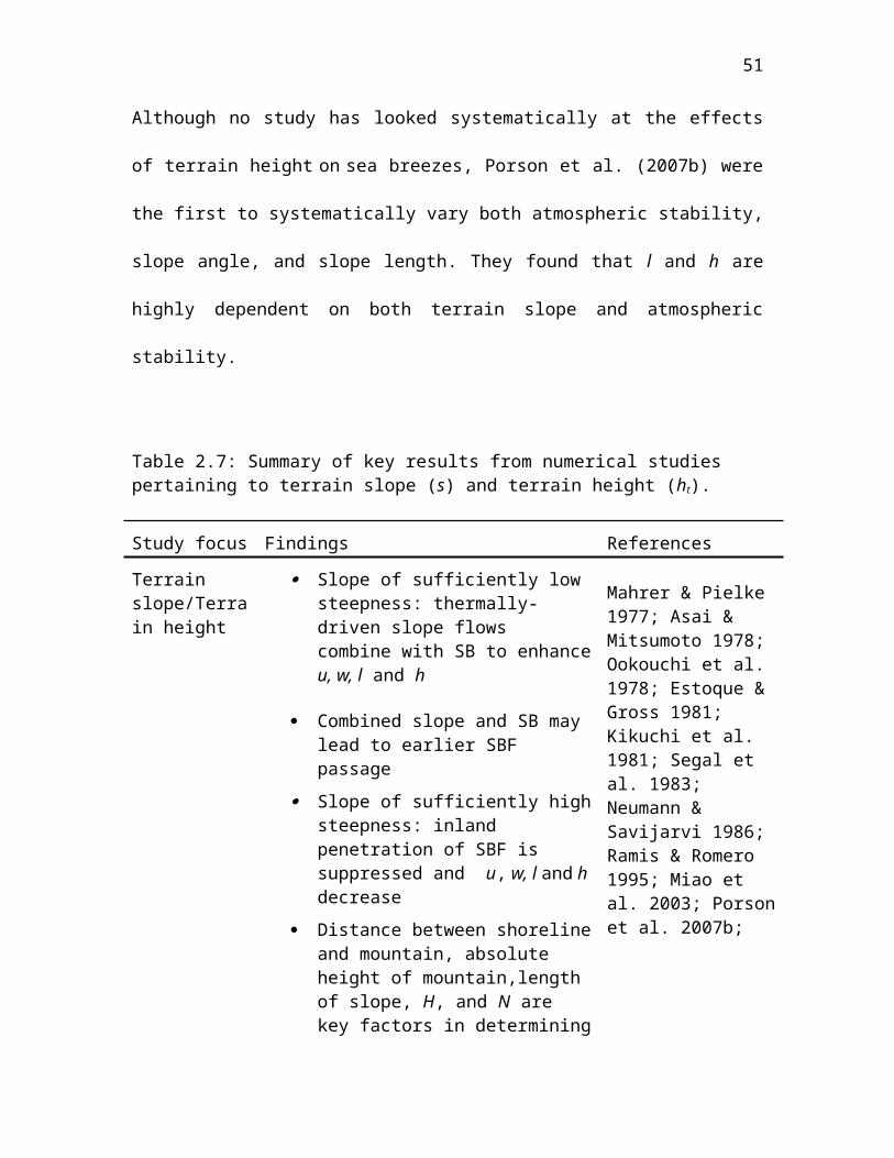
54
of the WRF model standard release so it is not included in this study. Antonnelli and
Rotunno (2007) made minor modifications to the TKE equation’s heat and momentum
eddy flux terms. The diffusive terms in the WRF model’s advective schemes have a
coefficient that is proportional to wind speed. At low wind speeds, the diffusion terms are
unable to remove poorly resolved features with wavelengths 2-4 times the grid spacing.
These spurious features can grow unless a filter is applied. The explicit 6th order
numerical diffusion option developed by Knievel et al. (2007) to preserve model
resolution while removing energy from spurious features is applied in this study.
Model Set-up for Control Simulation
The spatial configuration of what will hereafter be referred to as the
SEA_CONTROL simulation is illustrated in Fig. 3.1. A summary of the model set-up for
the SEA_CONTROL case is given in Table 3.2. The model was run in three dimensions,
with a volume of dimension 5 km (along-shore) x 230 km (cross-shore) x 5 km (vertical).
The horizontal grid resolution in the x and y dimensions were both 100 m, with 65
vertical levels stretched according to
grid (k )=
exp ( k−1float (k top−1 )
zscale)−exp( 1
zscale )1−exp( 1
zscale )
(3.1)
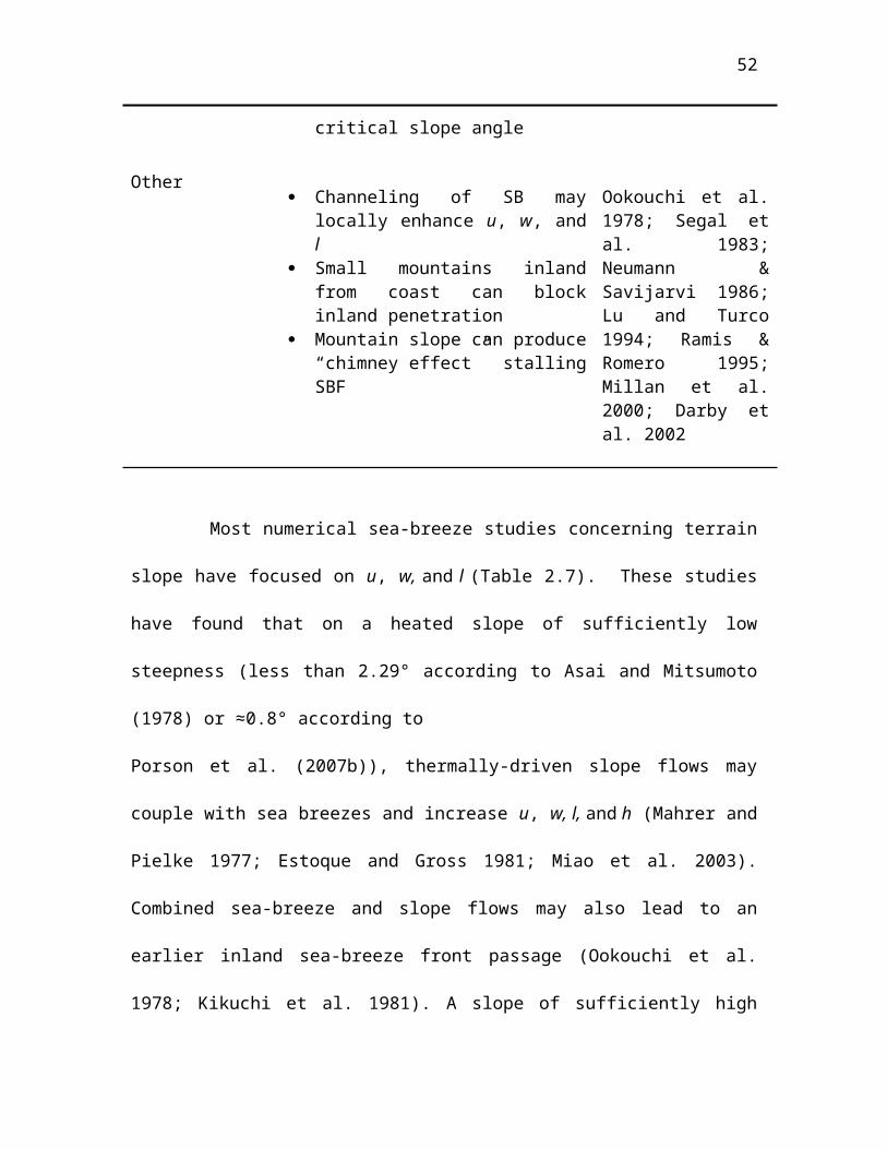
55
resulting in a vertical grid spacing which ranges from ~30 m at the lowest level to ~150
m at the model top. Periodic boundary conditions were imposed in the along-shore
direction with open boundary conditions in the cross-shore direction (Table 3.2). A 500
m deep W-Rayleigh damping layer was used at the model top to avoid reflection of
acoustic and gravity waves at the top of the model, although this may have been
unnecessary in the WRF model (Catalano and Moeng 2010). The model was run with a
56
unnecessary in the WRF model (Catalano and Moeng 2010). The model was run with a
57
Figure 3.1. Schematic diagram of sea breeze control simulation set-up.
58
Table 3.2: Overview of WRF control simulation settings.
WRF control simulation
Model parameter Selection
Domain230 km (x) x 5 km (y) x 4.5 km
(z)
x-direction 2300 grid points
x-grid spacing 100 m
y-direction 50 grid points
y-grid spacing 100 m
z-direction 65 grid points
z-grid spacing 30-150 m stretched Eqn. 3.1
Along-shore boundary-condition Periodic
Across-shore boundary-condition Open
Time step 1 s
Acoustic time step 0.166 s
Simulation length 10 hr
Damping layer W-Rayleigh
Damping coefficient 0.1
Damping layer depth 500 m
Initial atmospheric stability 0.01
Coriolis parameter 10-4 s-1
Initial geostrophic flow 0
Sensible heat flux over land According to Eqn. 3.2
Sensible heat flux over water 0 K m s-1
Roughness length over land 0.2 m
59
Roughness length over water 0.1 mm
1s time step (with 6 acoustic times steps for each time step) and was integrated for 10
hours. A time-varying land-surface sensible heat flux is prescribed by
heat flux ( t )=Asin( π12
)( t3600
) (3.2)
where t is the time in seconds from model initialization and A is the amplitude. The land
surface sensible heat flux according to Eq. 3.2 peaks after 6 hours. For the
SEA_CONTROL case, A was set to 0.16 K m s-1 (corresponding to a heat flux of ~180 W
m-2). The sensible heat flux was set to zero over water surfaces. Small negative sensible
heat fluxes observed over water due to evaporative cooling are neglected, since these
fluxes are typically an order of magnitude smaller than the land-surface sensible heat flux
(Segal et al. 1997).
A gradient of several grid boxes in the surface heat flux and drag was used to model
the transition between the lake and land surfaces. The aerodynamic surface roughness
length was prescribed to be 0.2 mm over water and 0.2 m over land (Table 3.2). A near-
standard initial atmospheric stability profile was used (Brunt-Viasala frequency N = 0.01
s-1) over the entire domain. The initial surface temperature was 288.15 K and the initial
background flow was set to zero. Spatial homogeneity in the initial vertical profiles of
temperature and background flow over both the land and water surfaces was assumed.
The Coriolis parameter f was set to 10-4 s-1. For the purposes of this study, hr 6
60
corresponds to roughly noon local solar time, with hr 10—the end of the simulation—
corresponding to midafternoon.
Control Simulation
The evolution of the modeled sea-breeze circulation from the SEA_CONTROL
simulation is shown in Fig. 3.2. The development and characteristics of the sea-breeze
system are consistent with observations and other LES studies. The low-level horizontal
sea-breeze flow initially forms just landward of the coastline and slowly deepens,
strengthens, and expands laterally over the land and water surfaces during the 10 hr
simulation, with a compensatory return flow observed aloft. The horizontal temperature
gradient associated with the sea breeze (ΔT between the coastline and the sea-breeze
front) increases from around 1 K at hr 3 to 5 K at hr 10. Along the leading edge of the
landward-moving sea-breeze gravity current there is no well-defined sea-breeze front,
with a horizontal temperature gradient of only 1 K (over 2-4 km) along the leading edge
of the sea-breeze flow. The frontolytical effects of convective boundary-layer turbulence
is hypothesized to be the cause of the relatively weak sea-breeze front.
An asymmetry in the horizontal distribution of the low-level onshore flow intensity
across the coastline is observed during most of the control simulation. During the
morning (hr 2-6), sea-breeze winds greater than 3 m s-1 are mostly confined to the land,
with weaker flow offshore. The expansion of horizontal velocities greater than 4 m s-1
occurs over twice as far of distance inland as offshore during the afternoon (Fig. 3.2).
The strongest low-level sea-breeze flow is located within 10 km of the coastline
through hr 8, 10-20 km behind the sea-breeze front in the region of the strongest
61
horizontal temperature gradient. The shoreline land-water temperature difference
weakens after hr 8 as the daytime heating wanes, shifting the strongest horizontal
62
Figure 3.2. Hourly y-averaged cross-coast wind speed (u, m s-1) and potential temperature ( θ, K) y-averaged for SEA_CONTROL experiment (see Table 3.2). Locations A-F indicate the
63
Figure 3.2 continued.
64
temperature gradient to the sea-breeze frontal region 20-40 km inland from the coast.
The intensification of the sea-breeze front at hr 10 is believed to be the result of
decreasing turbulent frontolysis of the horizontal land-water air temperature difference in
the mid-afternoon occurring as the land-surface sensible heat flux decreases. The onshore
flow at the coastline remains at a relatively constant depth (~600 m) through the
afternoon, while the depth of the horizontal flow far inland from the coastline increases
from 600 to near 1000 m during the afternoon behind the sea-breeze front (Fig. 3.2).
Fig. 3.3 shows a time series of the evolution of cross-coast velocities, temperature,
and pressure perturbations (between ocean and inland locations) at locations A-F in Fig.
3.2. Location F is located far enough inland that it does not feel the influence of the sea
breeze during the simulation and hence observes a steadily climbing temperature, light
and variable wind speeds, and falling surface pressure associated with convective heating
of the boundary-layer. At location A, located 12 km offshore, the horizontal sea-breeze
winds slowly increase during the afternoon as the circulation expands offshore, while the
near-surface temperature and pressure remain nearly constant. At the shoreline (location
B), the wind speeds increase during the morning into the early afternoon while the
temperature remains nearly constant due to the onshore flow of maritime air. At location
C, 4 km inland from the coast, a sea-breeze frontal passage is evident near hr 3, marked
by an increase in horizontal wind speed, and a flattening of the temperature trace. Further
inland, the sea-breeze frontal passage (locations D and E, located 12 and 24 km inland,
respectively) is later, which allows for greater morning heating of the boundary-layer and
development of the sea-breeze front with a pronounced 1.0 K temperature drop and rise
in surface pressure associated with frontal passage. The modifying influence of
65
in surface pressure associated with frontal passage. The modifying influence of
66
Figure 3.3. Time series of cross-coast velocity u (m s-1), potential temperature θ (K), and the pressure difference ΔP (hPa) between inland locations B, C, D, E and F and sea location A (see Fig. 3.2 for locations) at a height of 30 m AGL.
67
boundary-layer heating and turbulent convection on the sea-breeze gravity current can be se
n in the increasing temporal variability

CHAPTER 4
NUMERICAL SENSITIVITY STUDIES
Overview
Approximately fifty large-eddy simulations were conducted to determine the
sensitivity of sea- and lake-breeze wind intensity and inland extent to the land-surface
sensible heat flux (H), atmospheric stability (N), offshore background flow (Vg) , and
lake diameter (d) (Tables 4.1 and 4.2). These simulations were set up identically to the
SEA_CONTROL case except that the land-surface sensible heat flux, atmospheric
stability, background wind, and lake diameter were perturbed in each case. Periodic
rather than open boundary conditions were used at the lateral boundaries for the
background wind simulations to maintain numerical stability. A slab-symmetric lake was
centered in the model domain shown in Fig. 4.1 for the lake simulations. The model
domain in the x-direction was extended to 300 km for the large lake (d = 100 km). The
naming convention of the various sensitivity tests given in Tables 4.1 and 4.2 will be
used hereafter.
Four different lake diameters (d = 10, 25, 50, and 100 km) and the ‘infinite’ sea-
breeze dimension were used in this study. A slab-symmetric lake is used as shown in Fig.
4.1 of diameter d along the x-axis. The sea-breeze simulation configuration as shown in
Fig. 3.1 is considered an “infinite” dimension given the lateral open boundary conditions
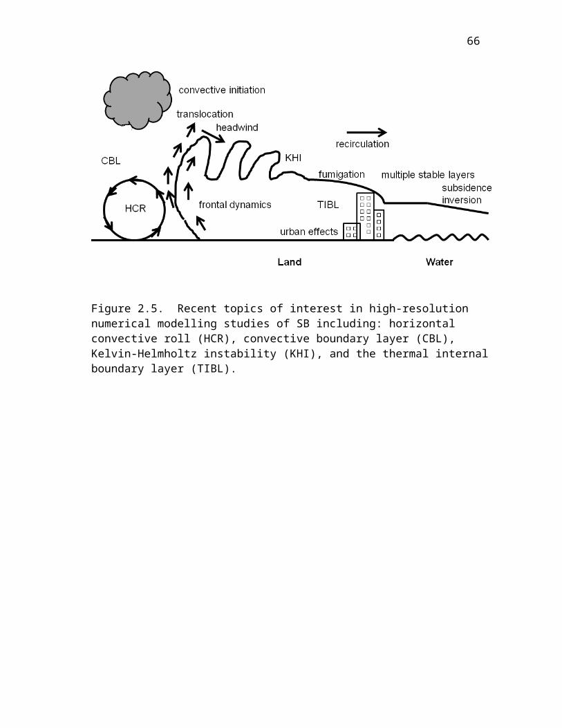
69
Table 4.1: LES Sensitivity Simulations Testing Variations in the Lake Diameter Land-Surface Sensible Heat Flux, Initial Atmospheric Stability, and Lake Diameter.
Case name Lake Diameter
(d, km)
Land-surface
sensible heat flux
(H, K m s-1)
Stability
(N, s-1)
SEA_CONTROL ∞ 0.16 0.01
SEA_LOW_H ∞ 0.08 0.01
SEA_HIGH_H ∞ 0.30 0.01
SEA_LOW_N ∞ 0.16 0.005
SEA_HIGH_N ∞ 0.16 0.02
10km_LAKE_CONTROL 10 0.16 0.01
10km_LAKE_LOW_H 10 0.08 0.01
10km_LAKE_HIGH_H 10 0.30 0.01
10km_LAKE_LOW_N 10 0.16 0.005
10km_LAKE_HIGH_N 10 0.16 0.02
25km_LAKE_CONTROL 25 0.16 0.01
25km_LAKE_LOW_H 25 0.08 0.01
25km_LAKE_HIGH_H 25 0.30 0.01
25km_LAKE_LOW_N 25 0.16 0.005
25km_LAKE_HIGH_N 25 0.16 0.02
50km_LAKE_CONTROL 50 0.16 0.01
50km_LAKE_LOW_H 50 0.08 0.01
50km_LAKE_HIGH_H 50 0.30 0.01
50km_LAKE_LOW_N 50 0.16 0.005
50km_LAKE_HIGH_N 50 0.16 0.02
70
100km_LAKE_CONTROL 100 0.16 0.01
100km_LAKE_LOW_H 100 0.08 0.01
100km_LAKE_HIGH_H 100 0.30 0.01
100km_LAKE_LOW_N 100 0.16 0.005
100km_LAKE_HIGH_N 100 0.16 0.02
Table 4.2: LES Sensitivity Simulations for Offshore Background Wind.
Case name Lake
Diameter
(d, km)
Land-surface
sensible heat
flux (H, K m s-1)
Stability
(N, s-1)
Backgroun
d Wind
(Vg,
m s-1 )
SEA_1MS ∞ 0.16 0.01 1
SEA_2MS ∞ 0.16 0.01 2
SEA_4MS ∞ 0.16 0.01 4
SEA_6MS ∞ 0.16 0.01 6
SEA_2MS_LOW_H_LOW_N ∞ 0.08 0.005 2
SEA_2MS_MED_H_LOW_N ∞ 0.16 0.005 2
SEA_2MS_HIGH_H_LOW_N ∞ 0.30 0.005 2
SEA_2MS_LOW_H_HIGH_N ∞ 0.08 0.02 2
SEA_2MS_MED_H_HIGH_N ∞ 0.16 0.02 2
SEA_2MS_HIGH_H_HIGH_N ∞ 0.30 0.02 2
SEA_2MS_MED_H_LOW_N ∞ 0.16 0.005 2
SEA_2MS_MED_H_HIGH_N ∞ 0.16 0.02 2
SEA_4MS_LOW_H_LOW_N ∞ 0.08 0.005 4
SEA_4MS_MED_H_LOW_N ∞ 0.16 0.005 4
71
SEA_4MS_HIGH_H_LOW_N ∞ 0.30 0.005 4
SEA_4MS_LOW_H_HIGH_N ∞ 0.08 0.02 4
SEA_4MS_MED_H_HIGH_N ∞ 0.16 0.02 4
SEA_4MS_HIGH_H_HIGH_N ∞ 0.30 0.02 4
SEA_4MS_MED_H_LOW_N ∞ 0.16 0.005 4
SEA_4MS_MED_H_HIGH_N ∞ 0.16 0.02 4
10km_LAKE_2MS 10 0.16 0.01 2
25km_LAKE_2MS 25 0.16 0.01 2
50km_LAKE_2MS 50 0.16 0.01 2
10km_LAKE_4MS 10 0.16 0.01 4
25km_LAKE_4MS 25 0.16 0.01 4
50km_LAKE_4MS 50 0.16 0.01 4
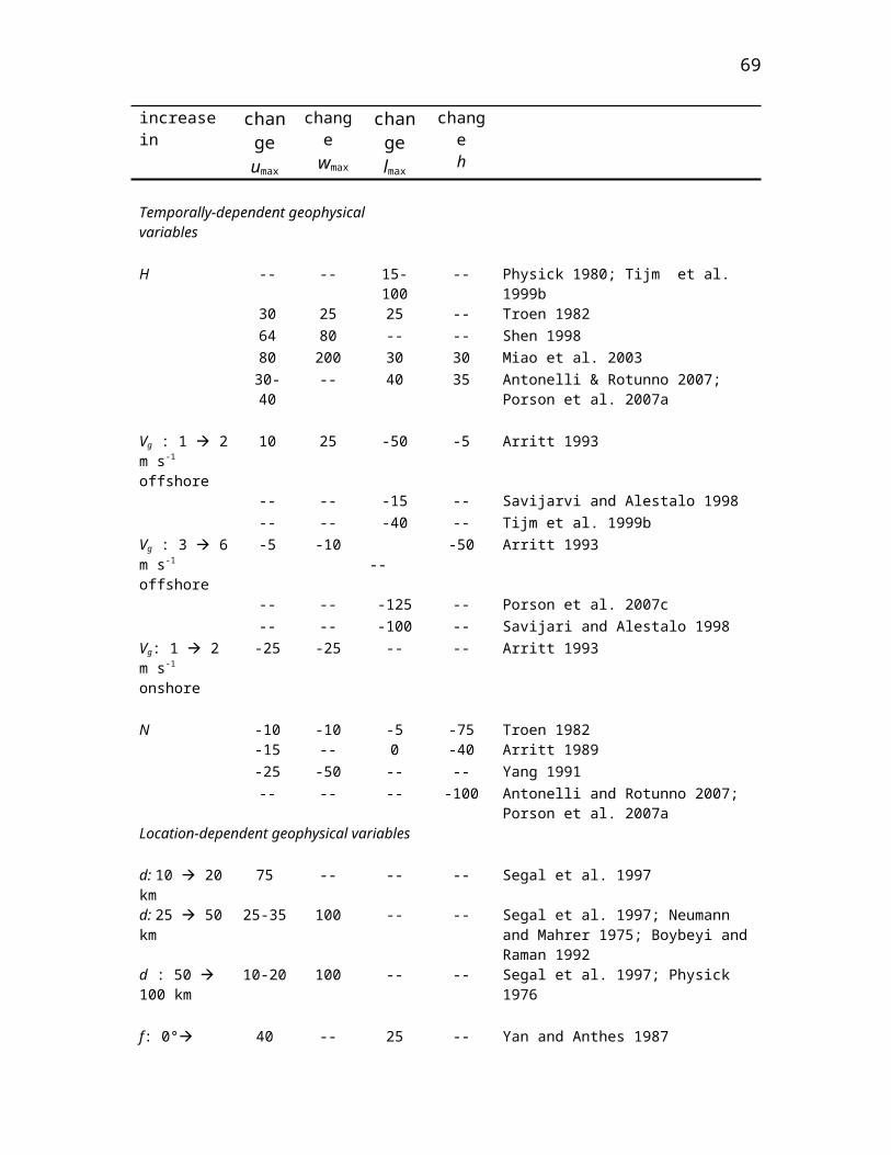
72
Figure 4.1. Schematic diagram of lake breeze simulation set-up.
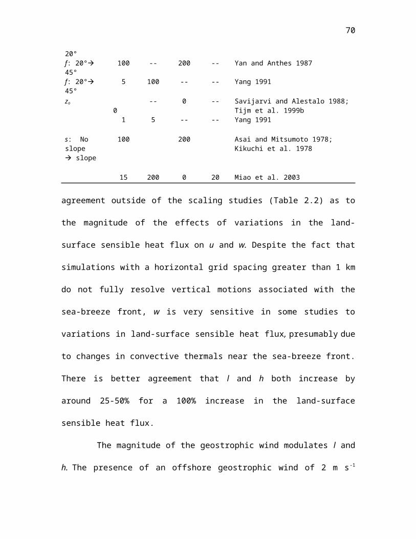
73
which allow an unlimited supply of cool air to advect in from the simulation boundary on
the lake side of the domain. For each of these five cases, a low, medium, and high land-
surface sensible heat flux (H = 0.08, 0.16, 0.30 K m s-1) and atmospheric stability
(represented by values of the Brunt-Viasala frequency N = 0.005, 0.01, 0.02 s-1) were
prescribed. The range of sensible heat fluxes used roughly correspond to those found in
low (~90 W m-2), medium (~180 W m-2), and high (~375 W m-2) land-surface sensible
heat flux environments (Hsu et al. 1983). Similarly, a range of initial stability profiles
were chosen with the intent of representing commonly observed atmospheric profiles. In
the weakly stably stratified environments specified with a low initial atmospheric
stability (N = 0.005 s-1), the lowest 1000 m of the boundary-layer mixes rapidly to near-
neutral stability in the presence of a high land-surface sensible heat flux, which is
representative of a sea or lake breeze forming in a hot, arid environment. The medium
value for the initial atmospheric stability (N = 0.01 s-1) is closer to that of a standard
atmosphere observed regularly in many coastal regions of the world. The high stability
case (N = 0.02 s-1) is more representative of an atmosphere with a preexisting marine
internal boundary-layer, deep nocturnal inversion, or elevated stable layer. Background
winds used in this study were prescribed initially from the offshore direction (flow that
opposes and is perpendicular to the sea-breeze flow) and of magnitude of 1, 2, 4, and 6 m
s-1. The initial flow was prescribed to be horizontally homogeneous and no wind shear
was specified with a constant wind speed between the top of the model domain and the
first grid point above the surface. Because of complex interactions between the offshore
winds, atmospheric stability, and the land-surface sensible heat flux, different
combinations of these three geophysical variables were conducted to better understand
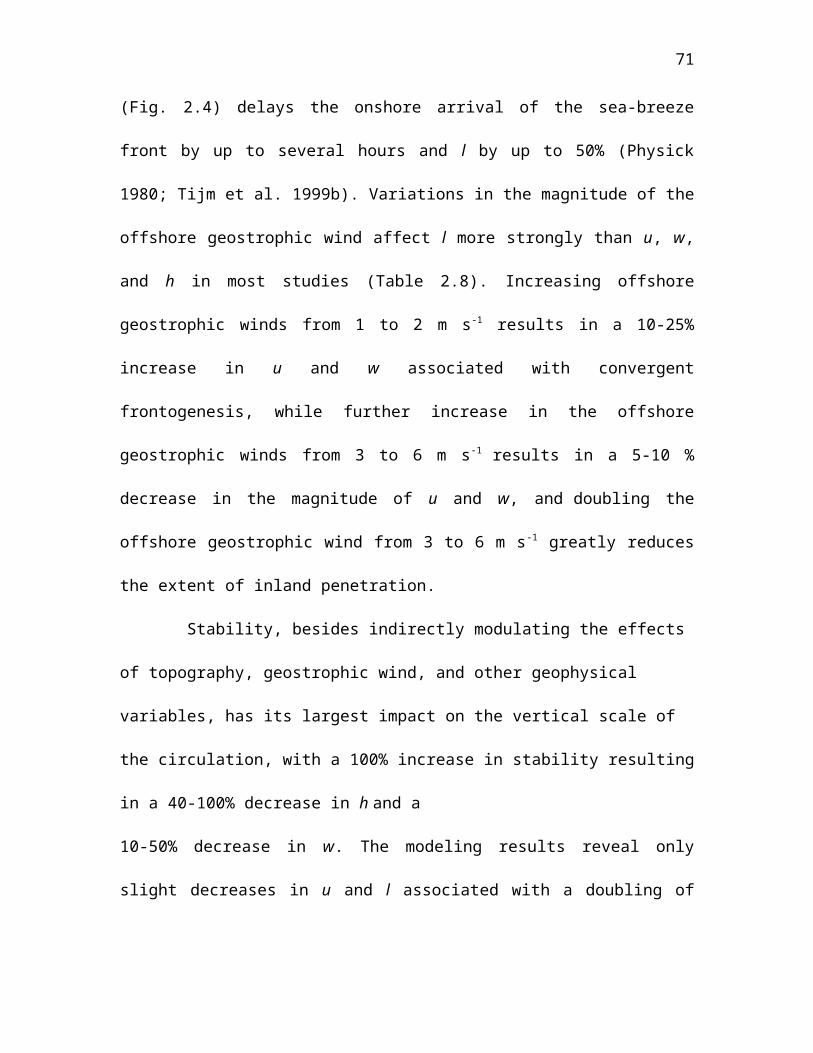
74
these relationships (Table 4.2). For offshore background flow greater than 4-6 m s-1, sea
or lake breezes are extremely shallow and/or may not occur depending on the size of the
lake or the magnitude of the land-surface sensible heat flux.
The sensitivity of the sea-breeze horizontal wind speed and inland extent to
variations in the geophysical variables depends on both time of day and the magnitude of
the geophysical variable being perturbed. In the following sections, we quantify the
cross-coast horizontal wind speed at the coastline (~30 m AGL) and the inland extent of
the sea-breeze front as a function of time of day and variations in the geophysical
variables.
Sensitivity to the Land-Surface Sensible Heat Flux
The sea-breeze horizontal wind intensity and inland extent are highly sensitive to
variations in the magnitude of the land-surface sensible heat flux (Fig. 4.2). For a
doubling of the land-surface sensible heat flux, there is a 25-50% increase in wind speed
and a 30-60% increase in inland extent depending on the time of day and the magnitude
of the sensible heat flux. For low values of the sensible heat flux, the peak horizontal
winds occur around hr 5.5 and remain relatively constant for the remainder of the
simulation. For medium and high land-surface sensible heat flux cases, peak horizontal
winds occur later near hr 7.5, with a larger relative decrease in the afternoon wind
intensity than in the low land-surface sensible heat flux case. The reason for the
differences in evolution between high and low land-surface sensible heat flux sea breezes
is likely related to the frontolytical effects of convective turbulence on the mature sea
breeze. Mechanical mixing due to intense surface heating dilutes the cool sea-breeze air
with warm heated air near the sea-breeze front, weakening the horizontal
75
Figure 4.2. Simulated cross-shore wind component u (ms-1) of breezes at the shoreline and inland extent l (km) for sea breezes for low (0.08 K ms-1), medium (0.16 K ms-1), and high (0.30 K ms-1) land-surface sensible heat flux cases. More details on cases in legend are available in Table 4.1.
76
thermodynamic temperature gradient and the subsequent horizontal pressure gradient and
inland rate of movement of the leading edge of the sea breeze. In a high sensible heat flux
environment, the thermodynamic temperature gradient across the sea-breeze front is
sufficiently strong (~4 K /10 km) that the sea-breeze front is only weakly affected by
turbulent frontolysis. In a low land-surface sensible heat flux environment, however, the
turbulent frontolysis likely has a larger relative impact on the weaker pre-existing
horizontal temperature gradient (~2 K /10 km).
The inland extent of the sea-breeze front also varies as a function of the land-surface
sensible heat flux. For a low land-surface sensible heat flux, the rate of inland movement
of the sea-breeze front is nearly constant for the entire simulation at approximately 5 km
h-1. For medium and high land-surface sensible heat flux, there is a notable acceleration in
the rate of inland movement of the sea-breeze front after hr 5, with the rate of inland
movement nearly 10 km hr-1 and 7.5 km hr-1 for the high and medium land-surface
sensible heat fluxes, respectively.
Variations in the land-surface sensible heat flux also impact the vertical and
horizontal scales of sea breezes, as well as the thermodynamics. Fig. 4.3 shows a cross-
section of the mature sea breeze (hr = 8) for low, medium, and high values of the land-
surface sensible heat flux. A larger land-water air temperature difference, more defined
sea-breeze front, and stronger horizontal low-level winds are associated with high versus
low land-surface sensible heat fluxes (Fig. 4.3a and c). The horizontal wind intensity is
also more uniform through the width of the sea-breeze circulation for a high land-surface
sensible heat flux than for a low sensible heat flux, where the strongest flow is confined
to the interior of the circulation. The offshore extent of moderate sea-breeze
77
to the interior of the circulation. The offshore extent of moderate sea-breeze
78
Figure 4.3. Cross-section of y-averaged sea breeze cross-coast wind speed (u, m s-1) and potential temperature (θ, K) for hr 8 for experiments a) SEA_LOW_H, b) SEA_CONTROL, c) SEA_HIGH_H, d) SEA_HIGH_N, e) SEA_LOW_N (see Table 4.1).
79
flow also appears to be a nonlinear function of the land-surface sensible heat flux, wit
h the circulation extending much further offshore for the high land-surface sensible heat
flux case. The vertical profile of sea-breeze wind intensity also varies with changes in
land-surface sensible heat flux and stability due to interactions with the cool low-leve
l gravity current. F or low land-surface sensible heat flux, the region of sea-breeze flow g
eater than 3.5 m s-1 in intensity is limited to 200 m depth, with 300 m of weaker flow
(< 2 m s-1) above. For high land-surface sensible heat flux, the depth of sea-breeze flo
w greater than 3.5 m s-1 expands to 600 m. However, the regio
The thermodynamic effects of variations in the land-surface sensible heat flux are
small near the shore as increases in the land-surface sensible heat flux are largely offset
by increased advection of cool oceanic air inland. Consequently, the surface air
temperature for low, medium, and high land-surface sensible heat fluxes remains nearly
constant for the first 10 km inland from the shoreline, but rise as a function of land-
surface sensible heat flux farther inland. The vertical expansion of the sea-breeze gravity
current through surface heating and turbulent mixing begins roughly 10 km inland from
the coast regardless of the initial atmospheric stability or magnitude of the land-surface
sensible heat flux.
Sensitivity to the Initial Atmospheric Stability
The sea-breeze horizontal wind intensity is weakly dependent on the initial
atmospheric stability while the inland extent is insensitive to stability (Fig. 4.4). Higher
stability results in a vertically-damped horizontal pressure gradient and slightly weaker
80
breeze intensity between simulation hrs 5 and 10. Between hr 2 and 5, the magnitude of
81
Figure 4.4. Simulated cross-shore wind component u (ms-1) of breezes at the shoreline and inland extent l (km) for sea breezes for low (0.005 s-1), medium (0.01 s-1), and high (0.02 s-1) atmospheric stability cases. More details on cases in legend are available in Table 4.1.
82
the wind speed is insensitive to the magnitude of the initial stability, likely because the
circulation is shallow enough that the vertical profile of temperature has little effe
t on the developing land-water horizontal temperature difference. However, betwe
n hr 5 and 10, a nearly linear dependence exists between stability and wind intensity. Thi
relationship presumably exists due to high stability case confining the vertical
xtent of the surface heating to a shallower layer near the ground, effectively limiti
Variations in the initial atmospheric stability distinctly impact the vertical and
horizontal scales of sea breezes, as well as the thermodynamics. Fig. 4.3b, d, and e show
cross-sections of the mature sea breeze (hr = 8) for low, medium, and high values of the
initial atmospheric stability. High atmospheric stability confines the depth of the low-
level sea-breeze flow greater than 3.5 m s-1 to around 300 m at the coastline, while low
stability allows that depth to be near 700 m.
In the case of high initial atmospheric stability, a greater near-surface land-water
temperature difference exists due to the confined heating of the low-levels in the stably-
stratified inland boundary-layer. However, the increased stability also vertically damps
the horizontal land-water air temperature difference, with this effect more than
compensating for the enhanced near-surface land-water temperature gradient, resulting in
an overall slight weakening of the circulation.
Sensitivity to the Offshore Background Wind
The interactions between the background wind and sea breezes are nonlinear and
complex. We focus in this study on the interactions between sea breezes and offshore
background wind as modulated by the magnitude of the land-surface sensible heat flux,
initial atmospheric stability, and lake diameter. Background winds flowing offshore
83
perpendicular to a coastline at speeds less than 5 m s-1 oppose the onshore-moving sea-
breeze gravity current and delay or stall the inland movement of the sea-breeze front,
typically resulting in convergent frontogenesis and a raised sea-breeze head (Chapter 2).
A graphical representation of the effects of the land-surface sensible heat flux and
initial atmospheric stability on the sea-breeze interaction with the offshore background
wind is given in Fig. 4.5. Both the amount of convergent frontogenesis along the sea-
breeze front and the turbulent mixing are a function of the magnitude of the initial
atmospheric stability, land-surface sensible heat flux, and the background wind. The
magnitude of the land-surface sensible heat flux fundamentally controls the amount of
differential heating and the overall depth and horizontal scale of the circulation.
However, there are complex interactions between the land-surface sensible heat flux and
the background flow. As the sea-breeze circulation deepens, the vertical footprint of the
interaction between the background flow and the sea breeze becomes larger and the
horizontal temperature gradient is subject to greater convergent frontogenesis. However,
as the depth of the sea breeze increases the vertical mixing of momentum from aloft into
the sea breeze increases and weakens the sea breeze. Similarly, the ambient stability
influences not only the depth of the sea breeze but also the amount of turbulence-induced
mixing at the top of the sea-breeze gravity current, hence modulating the mass exchange
between the sea breeze and the background flow. Our goal is to quantify the differences
in surface wind intensity, inland movement, and depth of the sea-breeze gravity current
as a function of offshore background wind.
84
Figure 4.5. Graphical representation of the interactions between the ambient background flow and atmospheric stability and land-surface sensible heat flux.
85
The sea-breeze horizontal wind intensity, inland extent, and depth are nonlinearly
dependent on the magnitude of the offshore background flow (Fig. 4.6). The effect of a
1-2 m s-1 offshore background wind on the sea-breeze horizontal wind intensity for the
first 6 hours of the sea-breeze life cycle is small, with a slight weakening in the afternoon
of the horizontal sea-breeze winds. When the offshore background wind is increased to 4
m s-1, the weakening effect on the sea breeze in the afternoon becomes more pronounced.
The onset of the sea breeze at the coast is also a function of offshore background wind
speed, occurring near hr 3 for an offshore background wind of 2 m s-1 and near hr 5 for an
offshore background wind of 4 m s-1 (Fig. 4.6).
An offshore background wind of 1 m s -1 decreases the midafternoon sea-breeze
inland extent and depth by nearly 20% with greater decreases for higher background
winds (Fig. 4.6). The sea-breeze flow is very weak and remains offshore for a
background wind of 6 m s-1 (Fig. 4.6) and no sea-breeze circulation forms when the
background winds are greater than 6 m s-1 (not shown). The depth of the sea-breeze low-
level flow decreases by 50% when the onshore background flow is increased from 2 to 4
m s-1 (Fig. 4.6).
Vertical cross-sections of the daytime life cycle of a sea breeze in the presence of
offshore background winds of 2 and 4 m s-1 are given in Figs. 4.7 and 4.8, respectively.
For the 2 m s-1 flow, the onshore horizontal extent is reduced compared to the zero wind
case (Fig. 3.2). The deepening of the sea-breeze flow with increasing distance inland
from the coast observed in the 0 m s-1 background wind case is largely absent in the 2 m
s-1 background wind case, except for a raised sea-breeze head (Fig. 4.7). The strongest
low-level horizontal winds associated with a 2 m s-1 offshore background wind are

86
Figure 4.6. Simulated cross-shore wind component u (ms-1) of breezes at the shoreline, inland extent l (km), and vertical depth h for sea breezes for 0,1,2,4, and 6 m s-1. More details on cases in legend are available in Table 4.1 and 4.2.
87
Figure 4.7. Evolution of sea breeze y-averaged cross-coast wind speed (u, m s-1) and potential temperature (θ, K) at hr 3, 6, and 9 for sea breeze with 2 m s-1 background ambient wind. Sea is represented by blue bracket.
88
Figure 4.8. Evolution of sea breeze y-averaged cross-coast wind speed (u, m s-1) and potential temperature (θ, K) at hr 3, 6, and 9 for sea breeze with 4 m s-1 background ambient wind. Sea is represented by blue bracket.
89
located just shoreward of the convergent frontogenesis (temperature gradient strengthens
immediately along the frontal boundary) compared to closer to the coast when no
offshore background flow is present (Fig. 4.2).
The effects of a 4 m s-1 offshore background flow on the daytime life cycle of a sea
breeze is shown in Fig. 4.8. Convergent frontogenesis along the nearly stationary sea-
breeze front has resulted in a 4 K horizontal temperature gradient over 5 km. However,
the vertical extent of the circulation has become negatively impacted by the increasing
offshore winds, with a stripping away of the upper portions of the gravity current near the
sea-breeze frontal region particularly apparent.
Offshore Background Wind and Land-Surface Sensible Heat Flux
The interactions between the magnitude of the land-surface sensible heat flux and the
ambient flow were tested for offshore background winds of 2 and 4 m s-1. The most
obvious difference between sea breezes forming with a 2 m s-1 offshore wind (Fig. 4.9)
and those forming with zero background flow (Fig. 4.2) is the delayed occurrence of the
arrival of the sea-breeze winds at the coastline with a 2 m s-1 offshore wind. The timing of
arrival of sea-breeze winds at the coast is a function of the magnitude of the land-surface
sensible heat flux (the sea-breeze circulation develops over open water due to the
opposing flow pushing the circulation seaward; when the circulation becomes strong
enough, it is able to move back to the shoreline). The intensity of the horizontal sea-
breeze winds between hrs 4 and 7 increase more rapidly for the 2 m s-1 offshore
background wind case (Fig. 4.9) than in the calm wind case (Fig. 4.2), presumably as a
consequence of convergent frontogenesis along the developing sea-breeze front.
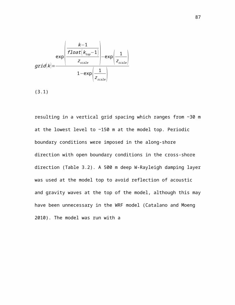
90
Figure 4.9. Cross-shore wind component u (m s-1) of breezes at the shoreline, inland extent l (km), and vertical depth h for sea breezes with 2 m s-1 opposing geostrophic flow for low, medium, and high land-surface sensible heat flux. More details on cases in legend are available in Table 4.2.

91
The inland extent of sea breezes with a 2 m s-1 background flow is roughly half that with
no background flow. The low heat flux cases exhibit a greater relative decrease in the
inland extent with a 2 m s-1 background flow (compared to zero background wind) than
high land-surface sensible heat flux cases (Fig. 4.9). The rate of inland movement of the
sea-breeze front remains relatively constant during the afternoon with an offshore
background wind of 2 m s-1, in contrast to the afternoon acceleration observed with a zero
background flow.
Further understanding of the interactions between the ambient background flow and
the land-surface sensible heat flux can be seen in a vertical cross-section of a sea breeze
with 2 m s-1 background flow for low, medium, and high values of the initial atmospheric
land-surface sensible heat flux (Fig. 4.10). The depth and intensity of the horizontal sea-
breeze flow near the sea-breeze front in the raised head region is enhanced with
increasing land-surface sensible heat flux from 0.08 to 0.16 K m s-1, presumably due to
convergent frontogenesis associated with the opposing 2 m s-1 background flow acting on
the larger land-water temperature difference. The enhancement of the low-level flow in
the frontal region is strongest when increasing the land-surface sensible heat flux from
low to medium values, while the largest enhancement of the entire sea-breeze circulation
occurs when the land-surface sensible heat flux is increased from medium to high values.
These spatial differences in wind intensity likely result from complex interactions
between the land-surface sensible heat flux-induced horizontal pressure gradient and the
offshore background flow. A maximum in horizontal wind speed is focused between the
sea-breeze front and the shoreline for low and medium land-surface sensible heat flux
cases, with significantly weaker winds over the water. For high sensible heat flux, there is
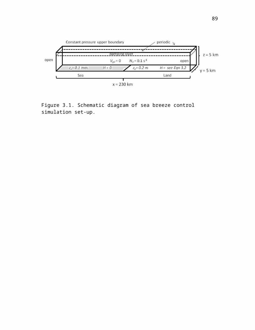
92
Figure 4.10. Cross-section of y-averaged sea breeze cross-coast wind speed (u, m s-1) and potential temperature (θ, K) for hr 8 for experiments with a 2 m s-1 opposing flow a) SEA_2MS_LOW_H_LOW_N, b) SEA_2MS_MED_H_LOW_N, c) SEA_2MS_HIGH_H_LOW_N (see Table 4.2). Sea is represented by blue bracket.
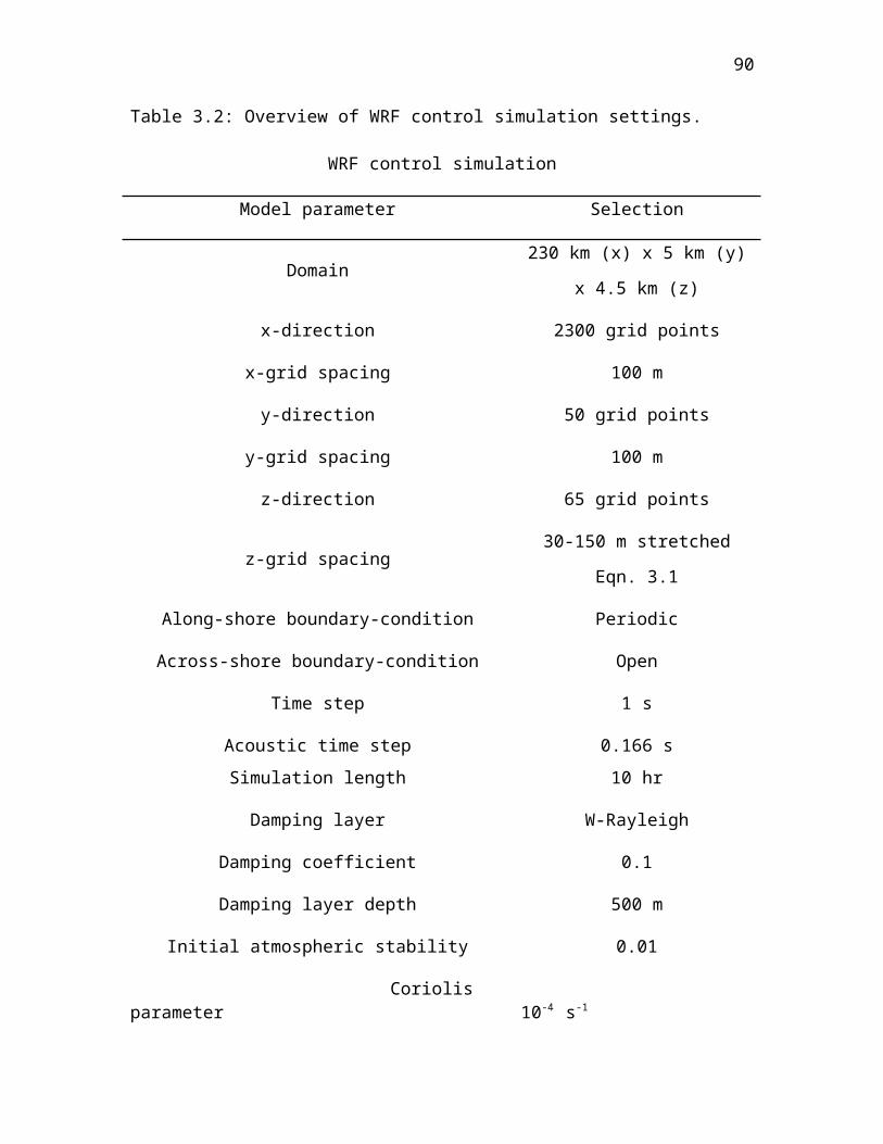
93
a slight weakening of the near-frontal wind intensity but the overall intensity of the
circulation over a broad region intensifies. The exact mechanisms for this are unclear but
have to do with interactions between the depth of the circulation imposed by the offshore
background wind, turbulent mixing at the top of the sea breeze, and the land-water air
temperature difference due to differential sensible heating of land and water surfaces.
The influence of variations in the magnitude of the land-surface sensible heat flux on
sea-breeze wind intensity, inland extent, and depth in the presence of a 4 m s-1
background flow are shown in Fig. 4.11. Vertical cross-sections at simulation hr 8 for the
same simulations are given in Fig. 4.12. A dramatic change in both the structure and
intensity of the sea breeze in the presence of a 4 m s-1 offshore background flow is seen
depending on the magnitude of the land-surface sensible heat flux (Fig. 4.12). For low
heat flux, the circulation is largely destroyed by turbulent interactions with the ambient
flow. However, for a high heat flux, the preexisting temperature gradient interacting with
the opposing flow allows for convergent frontogenesis along the sea-breeze front and a
raising of the sea-breeze head, which may also act to somewhat shield the downstream
sea breeze from turbulent mixing effects caused by wind shear between the sea-breeze
flow and opposing flow aloft. Variations in the land-surface sensible heat flux have
clearly nonlinear affects on the sea breezes in the presence of a 4 m s-1 background flow.
The sea breeze is weak, shallow, and remains offshore with a low land-surface sensible
heat flux but is significantly deeper and penetrates inland at ~1 km hr -1 during the
afternoon with a medium land-surface sensible heat flux. Further increases in the land-
surface sensible heat flux (from medium to high) results in a much stronger, deeper, and
faster moving sea-breeze front (Figs. 4.11 and 4.12).
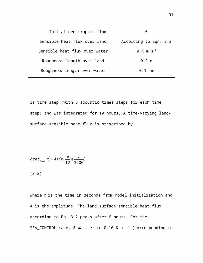
94
Figure 4.11. Simulated cross-shore wind component u (m s-1) of breezes at the shoreline, inland extent l (km), and vertical depth h for sea breezes with 4 m s-1 opposing geostrophic flow for low, medium, and high land-surface sensible heat flux. More details on cases in legend are available in Table 4.2.
95
Figure 4.12. Cross-section of y-averaged sea breeze cross-coast wind speed (u, m s-1) and potential temperature (θ, K) for hr 8 for experiments with a 4 m s-1 offshore wind a) SEA_4MS_LOW_H_LOW_N, b) SEA_4MS_MED_H_LOW_N, c) SEA_4MS_HIGH_H_LOW_N (see Table 4.2). Sea is represented by blue bracket.
96
Offshore Background Wind and Initial Atmospheric Stability
The sea-breeze horizontal wind intensity at the coast remains weakly sensitive to the
initial atmospheric stability and the inland extent remains insensitive to stability in the
presence of a 2 m s-1 offshore background wind (Figs. 4.13 and 4.14). Interactions
between the 2 m s-1 offshore flow and stability result in strengthening of the afternoon
low-level flow between the coastline and the sea-breeze front (Fig. 4.13a and b).
For a stronger offshore geostrophic wind (4 m s-1), the sensitivity of the horizontal
wind to variations in stability increases between hrs 6 and 8 (Figs. 4.15 and 4.16)
compared to the zero background wind case (Fig. 4.4). The sea-breeze inland extent is
also slightly delayed with low initial atmospheric stability (Fig. 4.15).
Variations in the initial atmospheric stability are associated with large variations in
the depth of the sea-breeze low-level flow (Figs. 4.13-4.16). The depth of the sea-breeze
low-level flow as the offshore background wind is increased from 2 to 4 m s-1 decreases
by approximately 50% for low, medium, and high values of the initial atmospheric
stability. Increasing stability with offshore background winds of 2 or 4 m s-1 also
confines the combined background flow and return circulation to a lower height, possibly
allowing for enhanced shear-induced turbulence at the top of the sea-breeze gravity
current (Figs. 4.13 and 4.14).
97
Figure 4.13. Simulated cross-shore wind component u (m s-1) of breezes at the shoreline, inland extent l (km), and vertical depth h for sea breezes with 2 m s-1 opposing geostrophic flow for low, medium, and high initial atmospheric stability. More details on cases in legend are available in Table 4.2.
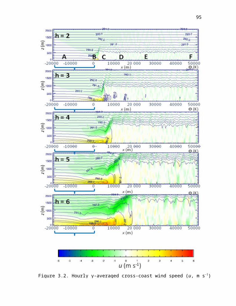
98
Figure 4.14. Cross-section of y-averaged sea-breeze cross-coast wind speed (u, m s-1) and potential temperature (θ, K) for hr 8 for experiments with a 2 m s-1 offshore wind a) SEA_2MS_MED_H_LOW_N, b) SEA_2MS_MED_H_MED_N, c) SEA_2MS_MED_H_HIGH_N (see Table 4.2). Sea is represented by blue bracket.
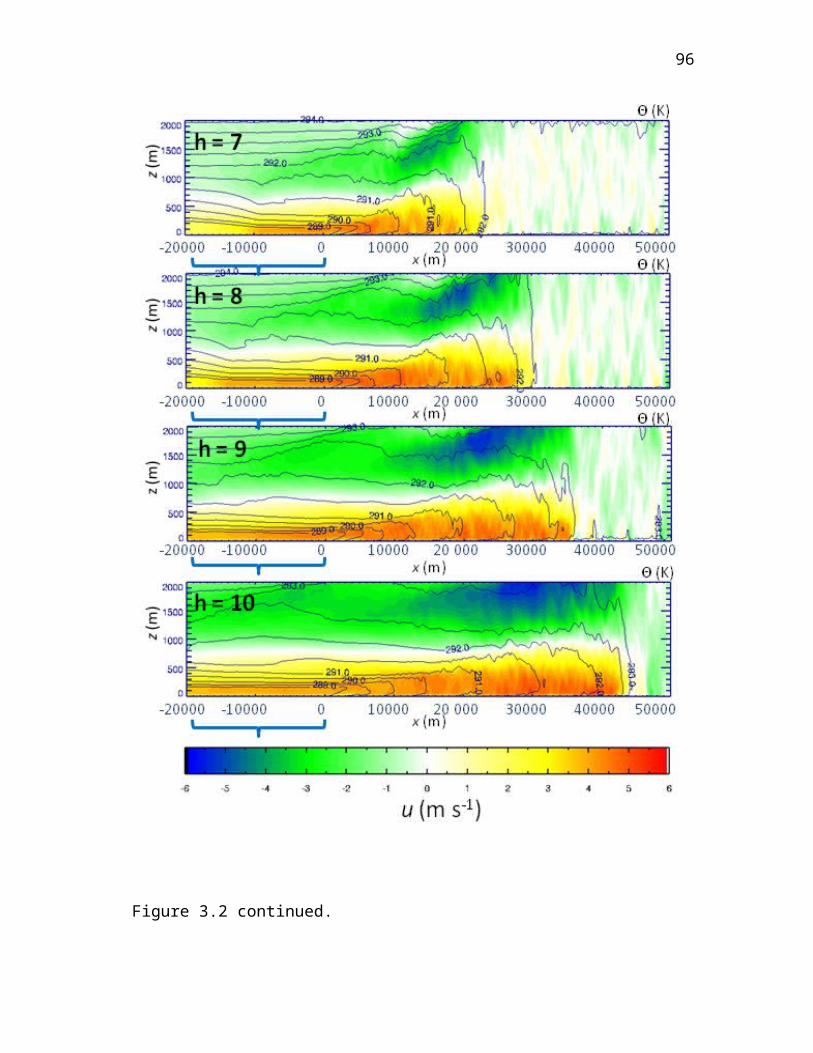
99
Figure 4.15. Simulated cross-shore wind component u (m s-1) of breezes at the shoreline, inland extent l (km), and vertical depth h for sea breezes with 4 m s-1 offshore geostrophic wind for low, medium, and high initial atmospheric stability. More details on cases in legend are available in Table 4.2.
100
Figure 4.16. Cross-section of y-averaged sea breeze cross-coast wind speed (u, m s-1) and potential temperature (θ, K) for hr 8 for experiments a) SEA_4MS_MED_H_LOW_N, b) SEA_4MS_MED_H_MED_N, c) SEA_4MS_MED_H_HIGH_N (see Table 4.2). Sea is represented by blue bracket.
101
Sensitivity to Lake Diameter
Lake diameter affects the intensity and inland extent of lake breezes through several
mechanisms. The size of a lake controls how much cool lake air is available for the lake
breeze in the afternoon. The available cool lake air may be largely consumed by breezes
associated with small and medium-sized lakes early in the afternoon, with compensatory
subsidence and associated warming over the lake weakening the land-lake temperature
difference and diminishing the lake-breeze flow (we will refer to this as “cool-air
limited”). The symmetric lake-breeze circulations forming on either side of the lake also
compete for available cool air and space over the water in which to grow laterally. For a
given lake diameter, the land-surface sensible heat flux, initial atmospheric stability, and
background wind further modulate how the available cool lake air is utilized by the lake
breeze, and how the offshore components of the symmetric breezes interact.
The lake-breeze horizontal wind intensity and inland extent are strongly dependent
on changes in lake diameter for small lakes and weakly dependent on changes in lake
diameter for medium to large lakes (Fig. 4.17). The magnitude of the lake-breeze
horizontal winds and inland extent decreases by over 50% as lake diameter decreases
from large (d=100 km) to very small (d=10 km). Large lakes have a horizontal flow and
inland extent nearly identical to sea breezes. The inland extent and lake-breeze wind
intensity associated with medium-sized lakes (d=50 km) are nearly identical to those of
large lake and sea breezes during the morning. During the late morning and afternoon, the
medium-sized lake-breeze circulation remains constant in intensity despite increased
land-surface heating as the available cool lake air is diminished. For small (d=25 km) and

102
Figure 4.17. Simulated cross-shore wind component u (m s-1) component of breezes at the shoreline and inland extent l (km) for lakes of diameter 10, 25, 50, and 100 km and the sea-breeze case d = ∞. Parameters used for these simulations can be found in Table 3 under the following cases: 10km_LAKE_CONTROL, 25km_LAKE_CONTROL, 50km_LAKE_CONTROL, 100km_LAKE_CONTROL, SEA_CONTROL.
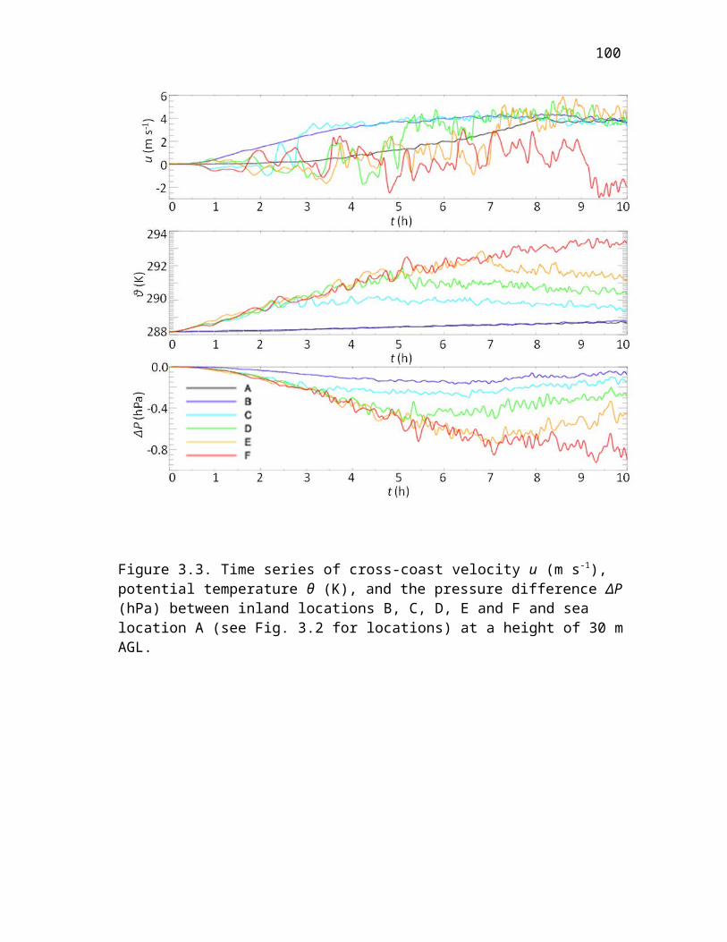
103
very small lakes (d=10 km), the lake breezes consume the available cool lake air early in
the day so that these breezes peak in intensity only 4 hrs into the simulation rather than
later in the afternoon.
The inland movement of the lake-breeze front for small and very small lakes is
nearly constant during the entire simulation, in contrast to the afternoon acceleration
noted for larger lakes (Fig. 4.17). This is likely due to the effects of turbulent frontolysis
on the weakened afternoon land-lake air temperature difference associated with smaller
lakes. There is a notable stalling of the small (d = 25 km) lake-breeze front during peak
heating and almost no inland movement of the very small (10 km diameter) lake-breeze
front between hr 5 and 9 (Fig. 4.17).
Lake Diameter and Land-Surface Sensible Heat Flux
The rate of depletion of the cool lake air for small and medium-sized lakes is
modulated by the magnitude of the land-surface sensible heat flux (Fig 4.18). A higher
land-surface sensible heat flux results in the lake consuming the available cool air earlier
in the day than for a low heat flux. For the first 5 hrs of lake-breeze development, the
low-level flow and inland extent are largely insensitive to lake diameter (for all but the 10
km lake) for both high and low magnitudes of the land-surface sensible heat flux.
In the case of a low land-surface sensible heat flux, the small lakes (d=10, 25 km)
become cool-air limited by hr 6 with substantial decreases in wind intensity and a
constant rate of inland movement of the lake-breeze front during the latter half of the
simulation. Lake breezes for larger lakes do not become cool-air limited with a horizontal
wind speed and rate of inland movement of the lake-breeze front similar to that of sea

104
Figure 4.18. Simulated cross-shore wind component u (m s-1) of breezes at the shoreline and inland extent l (km) for low (0.08 K m s-1) and high (0.30 K m s-1) land-surface sensible heat flux for lakes of diameter d = 10, 25, 50, and 100 km and the sea case d = ∞. Experiment names (see Table 4.1) are listed in the legend.
105
breezes (Fig. 4.18). The breeze intensity and inland penetration speed for low heat flux
cases also remains relatively constant after hr 5. It is unclear why sea and large lake
breezes do not intensify further after late-morning in the low land-surface sensible heat
flux case, except that the combination of a weaker onshore cool flow interacting with
weaker land-surface sensible heating some distance inland from the shore results in
frontolysis along the sea-breeze front, mitigating any further strengthening of the
circulation. Less intense surface heating in the low land-surface sensible heat flux cases
also results in fewer temporal fluctuations in the horizontal flow than in the high land-
surface sensible heat flux cases (Fig. 4.18).
For the high land-surface sensible heat flux cases, the wind speed and inland extent
for medium and large lakes begin to show some dependence on lake diameter
(although less than for the small lakes), as the larger circulations begin to deplete the
available cool lake air later in the afternoon. The 25 km diameter lake becomes cool-air
limited by hr 5 and the breeze wind intensity weakens substantially between hr 7 and 10.
The increase in inland extent for the 10 and 25 km diameter lakes as the land-surface
sensible heat flux is increased from low to high values is around 15 km, versus increases
of 20-30 km for larger lakes.
Lake Diameter and Atmospheric Stability
The sensitivity of lake breezes to variations in the initial atmospheric stability
follows that of sea breezes with a few caveats. The wind intensity of very small lakes
(d=10 km) is insensitive to variations in initial atmospheric stability as the lake becomes
cool-air limited when variations in stability begin to be important after simulation hr 5
(Fig. 4.19). Small and medium-sized lake (d=25, 50 km) wind intensity is slightly more
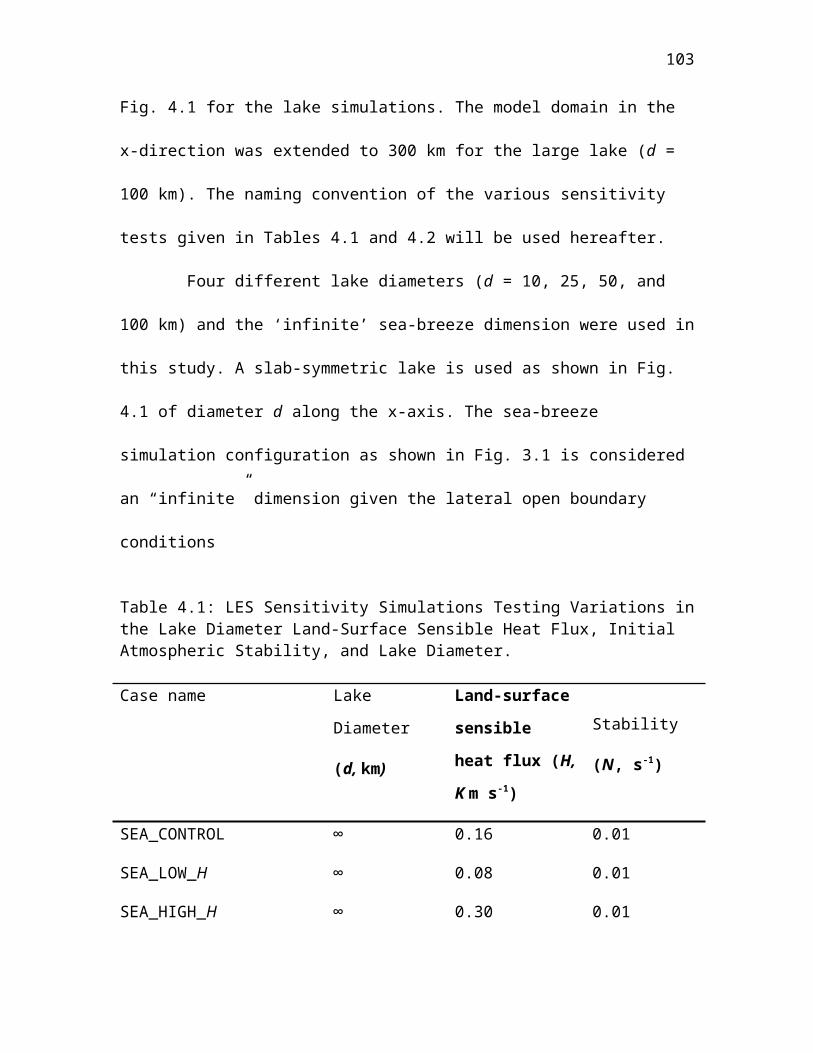
106
Figure 4.19. Simulated cross-shore wind component u (m s-1) of breezes at the shoreline and inland extent l (km) for low (0.005 s-1) and high (0.02 s-1) initial atmospheric stability for lakes of diameter d = 10, 25, 50, and 100 km and the sea case d = ∞. Experiment names (see Table 3) are listed in the legend.
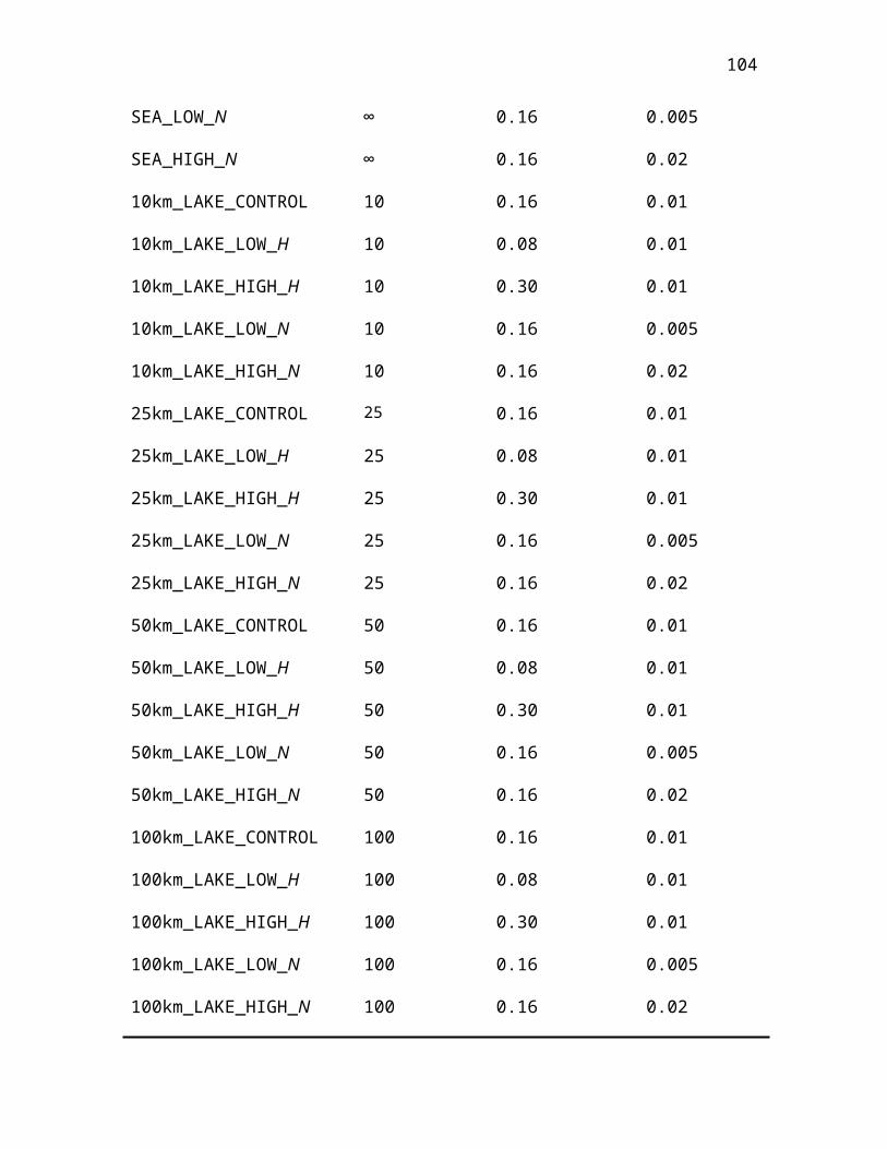
107
sensitive to variations in stability than for large lakes between hr 5 and 8 but less
sensitive between hr 9 and 10 (presumably due to the lakes becoming cool-air limited).
The inland extent of the lake breeze for small lakes (d=25 km) also varies as a function of
initial atmospheric stability in the afternoon, whereas for larger lakes, the influence of
stability on the inland extent remains small (Fig. 4.19).
Lake Diameter and Background Winds
The lake-breeze horizontal wind intensity and inland extent in the presence of a 4 m
s-1 opposing geostropic wind varies as a function of lake diameter (Fig. 4.20). For very
small lakes (d=10 km), the circulation is easily weakened by the opposing background
flow; a developing lake breeze is barely discernable, with weak, variable winds
(~ 1 m s-1), a very shallow low-level gravity current (~75 m depth), and virtually no
inland movement of the lake-breeze front (Fig. 4.20). The development of lake-breeze
circulations for lakes of 25, 50, and 100 km diameter are nearly identical during the
morning, with similar lake-breeze wind intensities, offshore extent (the breeze has not yet
reached shore), and depth for large and small lakes. It is not until the afternoon that the
lake-breeze circulation characteristics become a function of lake diameter. However, the
range of lake-breeze wind intensities between the small (d=25 km) and large (d=100)
diameter lakes is over 50% less than when there is zero geostrophic flow, indicating that
the opposing background wind fractionally weakens the large lake-breeze wind
intensities more than the small lake-breeze wind intensities. The inland extent of the 10
and 25 km diameter lakes after simulation hr 5 is reduced compared to the 50 km
diameter lake and sea breeze; however, even the large lake breeze is only able to
penetrate inland around 7 km in the presence of the 4 m s-1 offshore background wind.
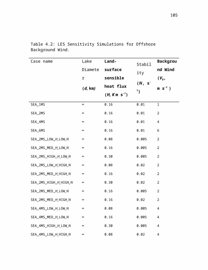
108
Figure 4.20. Simulated cross-shore wind component u (m s-1) of breezes at the shoreline, inland extent l (km), and vertical depth h for lake and sea breezes with 4 m s-1 opposing geostrophic flow. More details on cases in legend are available in Table 4.2.
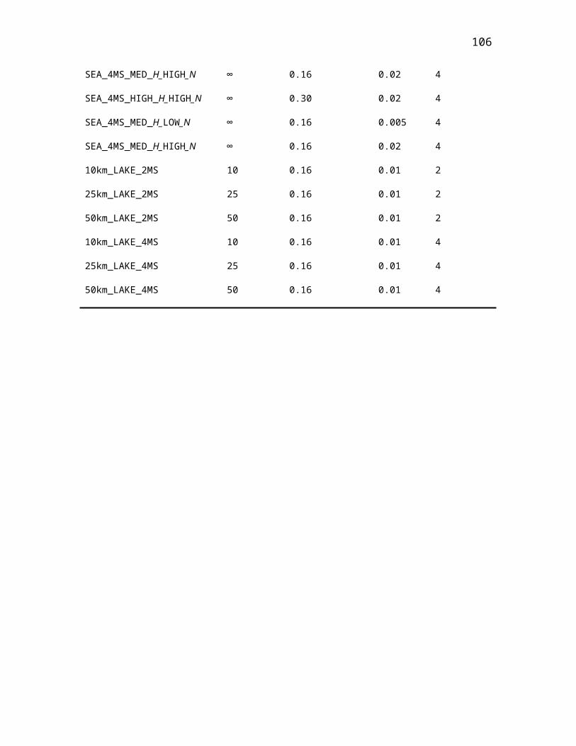
109
The depth of the low-level gravity current also varies as a function of lake diameter in the
afternoon, with progressively shallower lake breezes for smaller diameter lakes.
Differences Between Sea and Small Lake Breezes
Differences in the wind intensity and inland extent of small lake breezes compared to
sea breezes have been shown to exist. There are also notable differences in the spatial
structure of the low-level winds and the horizontal temperature gradients between land
and water associated with sea and lake breezes (Fig. 4.21). The most striking difference
between a small lake breeze (Fig. 4.21) and sea breeze (Fig. 4.3) is that the lake-breeze
circulation is horizontally and vertically smaller than the sea-breeze circulation. The land-
lake temperature differences associated with a mature small lake breeze are much weaker
than those associated with a mature sea breeze. The inland penetration of the lake-breeze
front is notably less than the sea-breeze front, and the lake- breeze front is less well-
defined. The maximum horizontal winds associated with the lake breeze are typically
confined to within 10 km of the shoreline but frequently extend beyond 20 km onshore
for the sea breeze. Because of the constraint of the symmetric lake-breeze cells
competing for space over the water, the offshore horizontal extent of the lake-breeze
circulation does not typically vary as a function of stability or heat flux like the sea
breeze. Finally, the low-level horizontal temperature gradient does not increase with
increasing heat flux for small lake breezes as it does in the sea-breeze case. On the
contrary, the midafternoon land-lake air temperature difference associated with the lake
breeze is weakened by a high land-surface sensible heat flux due to a lack of cool lake
air. In addition, due to the increased mixing over the land mass prior to (lake breeze is
delayed allowing for greater boundary-layer growth over land) and after sea-breeze
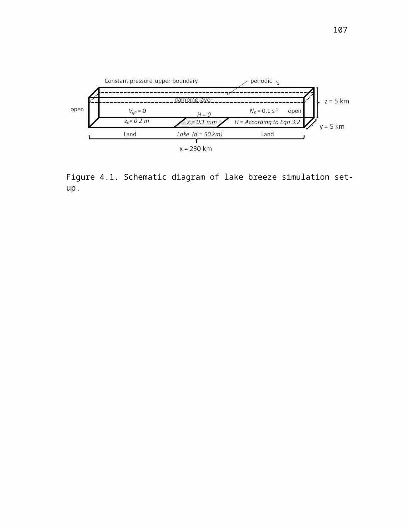
110
delayed allowing for greater boundary-layer growth over land) and after sea-breeze
111
Figure 4.21. Cross-section of y-averaged sea breeze cross-coast wind speed (u, m s-1) and potential temperature (θ, K) for hr 8 for experiments a) 25km_LAKE_LOW_H, b) 25km_LAKE_CONTROL, c) 25km_LAKE_HIGH_H, d) 25km_LAKE_HIGH_N, e) 25km_LAKE_LOW_N (see Table 3). 20 km of the 25 km diameter lake is shown (represented by blue brackets).
112
frontal passage (low-level flow off the small lake is mixed to greater depth than the mu
ch cooler sea-breeze flow), the depth of the small lake breeze associated with a high la
d-surface sensible heat flux is actually greater than the sea-breeze case in the imme
iate onshore region due to the weaker internal boundary layer associated w
Another way to compare the differences in horizontal structure between sea and lake
breezes is to compare the magnitude of the cross-coast wind speed between the shore and
locations on either side of the shore. As shown in Fig. 4.22, the horizontal flow 2 km
inland from the coast for sea breezes averages about 0.25 m s-1 weaker than at the coast
during the afternoon. However, the horizontal flow 2 km inland from the coast for small
lake breezes averages about 0.50 m s-1 stronger than at the lake shore during the
afternoon. Given that lake breezes for small lakes are only on the order of 2-3 m s -1, this
is a notable change in intensity over a small horizontal distance. For both sea and lake
breezes, the horizontal wind speeds associated with the sea breeze 6 km inland from the
coast are 0.5-1.5 m s-1 stronger than at the coastline. And while the sea-breeze flow 2 km
offshore tends to be similar to that at the shoreline, for small lakes, the flow 2 km
offshore is slightly weaker than at the shoreline.
113
Figure 4.22. Difference in cross-coast wind speed (u, m s-1) between shoreline location and locations 2 and 6 km onshore and 2 km offshore for SEA_CONTROL and 25km_LAKE_CONTROL experiments (see Table 4.1).
CHAPTER 5
SUMMARY AND FUTURE WORK
Numerical studies of sea and lake breezes have been reviewed and gaps in our
current understanding of these thermally-driven circulations were discussed. A series of
large-eddy simulations have been used to gain new insight into the sensitivity of the
daytime life cycle of the sea- and lake-breeze horizontal speed and length scales to
variations in the land-surface sensible heat flux, initial atmospheric stability, offshore
background wind, and lake diameter. Complex interactions between the various
geophysical variables have been shown to exist. Substantial spatial variability in the
intensity and vertical structure of sea- and lake-breeze circulations has been documented,
e.g., what is happening at the shoreline may be completely different from what is
happening several km onshore or offshore.
Sensitivity to Geophysical Variables
Sea- and lake-breeze horizontal wind intensity and inland extent are highly sensitive
to variations in the land-surface sensible heat flux, offshore background flow, and lake
diameter (for smaller lakes) and weakly sensitive to variations in the initial atmospheric
stability. As a way to summarize the effects of variations in these geophysical variables,
Table 5.1 lists the fractional change (i.e., change divided by the original value) in the
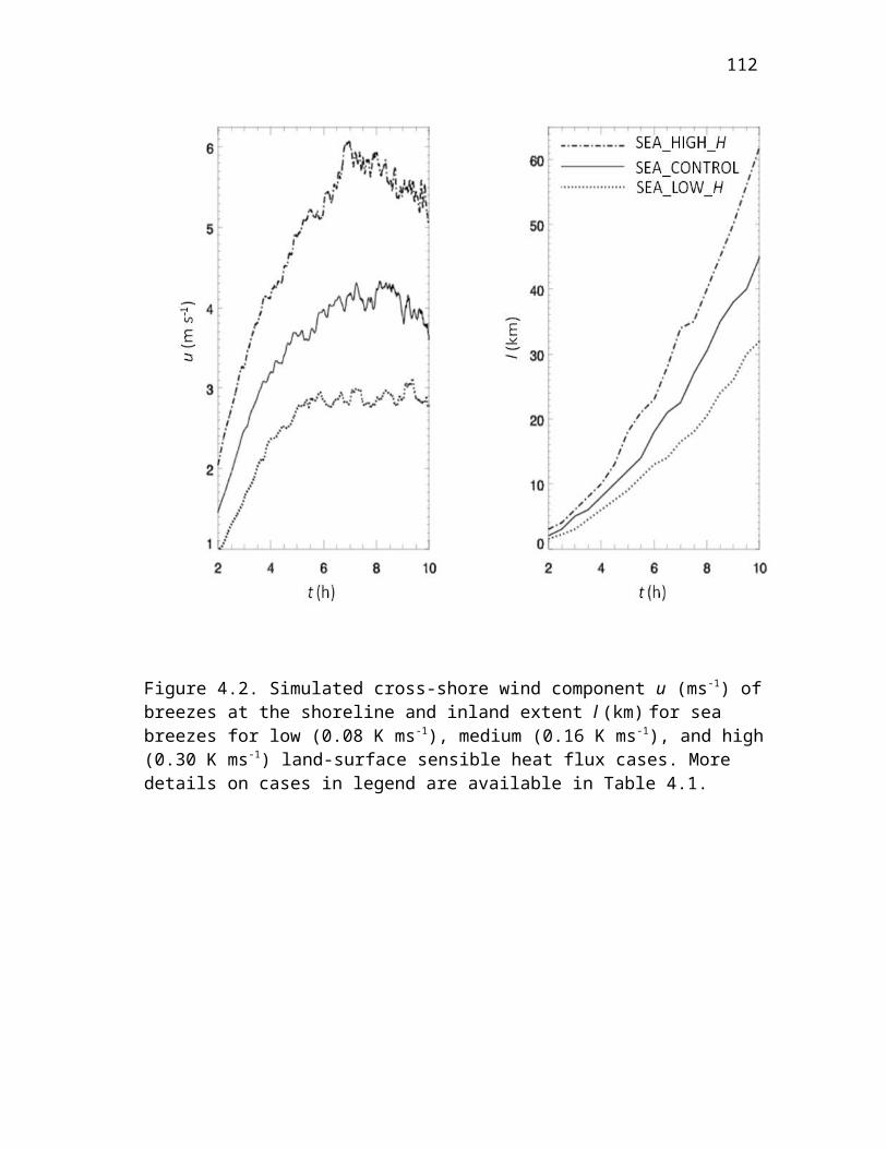
115
Table 5.1: Impact of a 100% increase in the geophysical variables on the developing mid-morning (hr 4) and mature midafternoon (hr 8) sea- and lake-breeze length (l) and velocity (u) scales expressed as the fractional change (change divided by original value). Geophysical variables are expressed as follows: Land-surface sensible heat flux (H), initial atmospheric stability (N), water body dimension (d), and constant background opposing flow (V). Arrow () denotes a specific doubling of a geophysical variable.
100% increase in
hr 4% change
u
hr 4 %
change L
hr 8%
changeu
hr 8% change
l
Cases compared
H Sea Breeze0.08 0.16 45 40 50 60 SEA_LOW_H; SEA_CONTROL0.16 0.30 35 40 35 40 SEA_CONTROL; SEA_HIGH_HH 50 km lake0.08 0.16 30 100 40 35 50km_LAKE_LOW_H;
50km_LAKE_CONTROL0.16 0.30 33 43 29 40 50km_LAKE_CONTROL;
50km_LAKE_HIGH_HH 25 km lake0.08 0.16 40 75 50 16 25km_LAKE_LOW_H;
25km_LAKE_CONTROL0.16 0.30 30 43 40 47 25km_LAKE_CONTROL;
25km_LAKE_HIGH_HH 10 km lake0.08 0.16 30 25 30 0 10km_LAKE_LOW_H;
10km_LAKE_CONTROL0.16 0.30 25 40 -- 44 10km_LAKE_CONTROL;
10km_LAKE_HIGH_H
N Sea Breeze0.005 0.01 -2 0 -10 0 SEA_LOW_N; SEA_CONTROL0.02 0.02 -2 -2 -9 0 SEA_CONTROL; SEA_HIGH_NN 50 km lake0.005 0.01 0 0 0 -15 50km_LAKE_LOW_N;
50km_LAKE_CONTROL0.02 0.02 -10 0 -14 -7 50km_LAKE_CONTROL;
50km_LAKE_HIGH_NN 25 km lake0.005 0.01 -3 0 -7 -20 25km_LAKE_LOW_N;
25km_LAKE_CONTROL0.02 0.02 -4 0 -18 0 25km_LAKE_CONTROL;
25km_LAKE_HIGH_NN 10 km lake0.005 0.01 0 0 0 -25 10km_LAKE_LOW_N;
10km_LAKE_CONTROL0.02 0.02 0 0 0 13 10km_LAKE_CONTROL;
10km_LAKE_HIGH_N
d: 10 25 km
22 50 23 65 10km_LAKE_CONTROL; 25km_LAKE_CONTROL
d: 25 50 km
5 12 30 25 25km_LAKE_CONTROL; 50km_LAKE_CONTROL
d : 50 100 km
3 -12 20 15 50km_LAKE_CONTROL; 100km_LAKE_CONTROL
d: 100 sea 2 0 2 15 100km_LAKE_CONTROL; SEA_CONTROL
Vg0 1m s-1 0 -30 0 -30 SEA_CONTROL; SEA_1MS1 2m s-1 0 -50 -10 -25 SEA_1MS; SEA_2MS2 4m s-1 -- -100 -20 -75 SEA_2MS; SEA_4MS
116
horizontal length and velocity scales of lake and sea breezes to 100% increases in the
magnitudes of the geophysical variables at simulation hr 4 and 8. In most cases, the
results agree with previous numerical and observational scaling studies on the magnitude
of the sensitivity of sea breezes to variations in the geophysical variables during the
mature phase of the sea breeze (Table 2.8). However, no previous study has summarized
the temporally-varying impacts of these variables over the daytime breeze life cycle, so
comparisons cannot typically be made at other times.
Sensitivity to Land-Surface Sensible Heat Flux and Initial Atmospheric Stability
A 100% increase in the land-surface sensible heat flux results in a 35-50% increase
in the sea-breeze horizontal winds and a 40-60% increase in the inland extent of the sea-
breeze front (Table 5.1). For smaller lakes, a 100% increase in the land-surface sensible
heat flux results in a generally smaller increase in the lake-breeze inland extent due to
interactions between lake diameter (available cool air) and the land-surface sensible heat
flux (Table 5.1). The modeled sensitivity of sea-breeze horizontal winds to the land-
surface sensible heat flux (Fig. 4.2; Table 5.1) is consistent with existing scaling analyses
and several numerical studies that predict horizontal sea-breeze wind speeds to vary
according to √H (Tables 2.2 and 2.8). However, the detailed temporal evolution of the
horizontal wind intensity as a function of heat flux (e.g., no afternoon increase in wind
intensity for low heat flux cases but substantial increases for high heat flux case) is not
captured by current scaling relations.
The afternoon acceleration of the sea-breeze front inland noted in observations and in
these LES (Fig. 4.2) is not observed in several previous course-resolution modeling
117
studies (Fig. 2.4). Scaling analyses such as that of Steyn (1998) which give inland extent
as a linear function of the land-surface sensible heat flux do not include this afternoon
acceleration of the sea-breeze front. While there is some indication of slowing of the
inland movement of the sea-breeze front near peak daytime heating due to turbulent
frontolysis effects (Chapter 2; Fig. 4.2), the LES indicate that the pronounced slowing of
the sea-breeze front noted in a few earlier numerical studies may be unrealistic. However,
the effect of turbulent frontolysis on slowing the rate of inland acceleration of the sea-
breeze front is inherent in these results: a doubling of the land-surface sensible heat flux
from 0.16 to 0.30 K m s-1 only results in a 40% increase (not 100%) in the midafternoon
inland extent.
Increasing the land-surface sensible heat flux at the coastline has a small impact on
the local temperature at the coast as the stronger sea-breeze circulation allows for greater
advection of cool maritime air inland, offsetting the local warming (Fig. 4.3a-c).
Consequently, the local effects of anthropogenic land-surface changes (e.g.,
deforestation, desertification) on coastal temperature may be partially offset by the
induced changes in sea-breeze wind intensity.
The weak sensitivity of sea-breeze horizontal wind intensity and inland extent to
variations in atmospheric stability (Table 5.1; Fig. 4.4) is consistent with several previous
modeling studies and suggests that linear theory may overpredict the sensitivity of sea-
breeze horizontal extent to variations in initial atmospheric stability (Eq. 2.2). The
temporal variability in the sensitivity of sea breezes to variations in the initial static
stability (sea-breeze horizontal winds are insensitive to stability during the first 5 hrs) has
not been previously documented.

118
Sensitivity to Offshore Background Wind
The sensitivity of sea-breeze horizontal wind and length scales to variations in the
background wind increases with increasing magnitude of the background flow (Table 5.1;
Fig. 4.6). Increasing the background offshore wind from 0 to 1 m s-1 has no impact on the
sea-breeze horizontal winds and results in a 30% decrease in the inland extent of the sea-
breeze front (Table 5.1). Increasing the offshore background wind from 1 to 2 m s-1
results in a 10% decrease in the sea-breeze horizontal wind intensity and a 25-50%
decrease in the sea-breeze inland extent (Table 5.1). Further increasing the offshore
background wind from 2 to 4 m s-1 results in a 20% decrease in the sea-breeze horizontal
winds and a 50-100% decrease in the sea-breeze inland extent. The sea-breeze inland
extent is slightly more sensitive to variations in the background wind in the morning than
in the afternoon.
Complex interactions have been shown to occur between the background flow, land-
surface sensible heat flux and initial atmospheric stability; these relationships have been
largely neglected in previous studies. Complex interactions were found to exist between
the opposing background wind and the land-surface sensible heat flux. Interactions
between the initial atmospheric stability and the offshore winds existed but were weaker.
The intensification of sea-breeze fronts with increasing offshore background winds was
less in the LES simulations than in earlier coarse-resolution models. These differences
indicate that turbulent frontolysis and other weakening effects may be underrepresented
in coarse-resolution models. Perhaps as a consequence of the limitations of earlier
coarse-resolution models, the critical value of the offshore background wind in our study
of 6 m s-1 (above which no sea breeze forms) was lower than the 7-11 m s-1 discussed in
119
the previous modeling literature.
Previous to this study, the effects of increasing offshore flow on the depth of sea
breezes were unclear and underestimated. The depth of the sea breeze is highly sensitive
to increases in the offshore background flow, with a 1 m s-1 offshore background flow
decreasing the sea-breeze depth by 20% and a 4 m s -1 offshore background flow
decreasing the sea-breeze depth by 70%.
Sensitivity to Lake Diameter
This is the first study to investigate the combined influence of lake diameter, land-
surface sensible heat flux, and initial atmospheric stability on lake breezes. The
sensitivity of lake-breeze horizontal wind and length scales to variations in the lake
diameter increases with decreasing lake size (Table 5.1; Fig. 4.17). Increasing the lake
diameter from 10 to 25 km results in a 20% increase in the lake-breeze horizontal winds
and a 50% increase in the lake-breeze inland extent (Table 5.1). Further increasing the
lake diameter from 50 to 100 km results in only around a 10% increase in both the lake-
breeze horizontal winds and inland extent. The sensitivity of lake-breeze horizontal wind
intensity and inland extent to lake diameter is modulated by the land-surface sensible heat
flux and background wind (Figs. 4.18 and 4.19).
Lake breezes associated with small lakes reach their maximum intensity several
hours earlier than sea breezes (Fig. 4.17). These lake breezes also weaken in the
afternoon when sea breezes typically observe their highest wind speeds. In response to
the weakening afternoon lake breeze, the rate of inland movement of a small lake-breeze
front does not accelerate in the afternoon as does the sea-breeze front. The strongest
horizontal lake-breeze winds are confined closer to the shore than is the case for sea
120
breezes. Sea-breeze scaling laws are clearly not appropriate for lake breezes associated
with small lakes in the afternoon when the available cool lake air has been largely
consumed.
Future Work
The modeled dependence of sea and lake breezes to variations in geophysical forcing
have been presented thus far in terms of two simple measures of sea- and lake-breeze
intensity: the horizontal length and speed scales. These simple measures were used
because they allow for rapid initial evaluation of over 50 simulations and inter-
comparison between the LES and previous coarse-resolution numerical studies and
observational scaling analyses. There exists a plethora of information regarding lake- and
sea-breeze spatiotemporal structure inherent in the LES that cannot be gleaned from an
analysis of u and l. More sophisticated analysis methods will follow in the future.
Much analysis remains to better quantify and evaluate the LES results. Scaling
analyses are needed, particularly for lake breezes. Further modeling sensitivity studies are
necessary to diagnose the interactions between lake diameter and geostrophic flow as
modulated by the initial atmospheric stability and land-surface sensible heat flux.
Determining the critical value of the offshore background flow above which no sea or
lake breeze is able to form (listed in the literature between 4-11 m s-1 with much
uncertainty) as a function of lake diameter and other geophysical variables is also of
interest. Quantification of sea- and lake-breeze volume flux, vertical motion along the
sea-breeze front, and depth of both the low-level gravity current and return flow aloft as a
function of the various variables would also be useful for air quality research. Further
investigation into the offshore wind intensity and extent in the presence of variations in
121
these variables is necessary for offshore wind energy applications. As discussed earlier,
the strongest flows associated with lake and sea breezes are typically located some
distance inland from the coast. Future research could quantify both the location of the
“maximum” sea-breeze flow under different conditions and the location inland where the
laminar onshore gravity current becomes dominated by convective eddies in the
developing internal boundary layer. Such results would be useful for both air quality and
wind energy interests.

REFERENCES
Abbs DJ (1986) Sea-breeze interactions along a concave coastline in Southern Australia: Observations and numerical modeling study. Mon Weather Rev 114:831–848
Abbs DJ, Physick WL (1992) Sea-breeze observations and modelling: a review. Aust Meteorol Mag 41:7-19
Ado HY (1992) Numerical study of the daytime urban effect and its interaction with the sea-breeze. J Appl Meteorol 31:1146-1164
Alpert P, Cohen A, Neumann J, Doron E (1982) A model simulation of the summer circulation from the Eastern Mediterranean past Lake Kinneret in the Jordan Valley Mon Weather Rev 110:994–1006
Anthes RA (1978) The height of the planetary boundary layer and the production of circulation in a sea breeze model. J Atmos Sci 35:1231–1239
Antonelli M, Rotunno R (2007) Large-eddy simulation of the onset of the sea breeze. J Atmos Sci 64:4445-4457
Arritt RW (1987) The effect of water surface temperature on lake breezes and thermal internal boundary layers. Boundary-Layer Meteorol 40:101–125
Arritt RW (1989) Numerical modelling of the offshore extent of sea breezes. Q J Roy Meteorol Soc 115:547-570
Arritt RW (1993) Effects of the large-scale flow on characteristic features of the sea breeze. J Appl Meteorol 32:116–125
Asai T, Mitsumoto S (1978) Effects of an inclined land surface on the land and sea breeze circulation: A numerical experiment. J Meteorol Soc Jpn 56:559-570
Asimakopoulos DN, Helmis CG, Papadopoulos KH, Kalogiros AJ, Kassomenos P, Petrakis M (1999) Inland penetration of sea breeze under opposing offshore wind. Meteorol Atmos Phys 79:97-110
Atkins NT, Wakimoto RM, Weckwerth TM (1995) Observations of the sea-breeze front during CaPE. Part II: dual-doppler and aircraft analysis. Mon Weather Rev 123:944–969
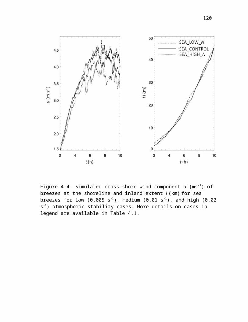
123
Atkinson BW (1981) Meso-scale atmospheric circulations. Academic Press, London, 495 pp
Avissar R, Moran MD, Wu G, Meroney RN, Pielke RA (1990) Operating ranges of mesoscale numerical models and meteorological wind tunnels for the simulation of sea and land breezes. Boundary-Layer Meteorol 50:227-275
Baker RD, Lynn BH, Boone A, Tao WK, Simpson J (2001) The influence of soil moisture, coastline curvature, and land-breeze circulations on sea-breeze-initiated precipitation. J Hydrometeorol 2:193–211
Banta RM, Olivier LD, Levinson DH (1993) Evolution of the Monterey Bay sea-breeze layer as observed by pulsed Doppler radar. J Atmos Sci 50:3959-3982
Bechtold P, Pinty JP, Mascart P (1991) A numerical investigation of the influence of large-scale winds on sea-breeze and inland-breeze type circulations. J Appl Meteorol 30:1268–1279
Biggs WG, Graves ME (1962) A lake breeze index. J Appl Meteorol 1:474–480 Bitan A (1977) The influence of the special shape of the Dead Sea and its influence on the
local wind system. Arch Met Geoph Biokl 24:283-301.
Briere S (1987) Energetics of daytime sea breeze circulation as determined from a two-dimensional, third-order turbulence closure model. J Atmos Sci 44:1455–1474
Boybeyi Z, Raman S (1992a) A three-dimensional numerical sensitivity study of mesoscale circulations induced by circular lakes. Meteorol Atmos Phys 49:19-41
Boybeyi Z, Raman S (1992b) A three-dimensional numerical sensitivity study of convection over the Florida peninsula. Boundary-Layer Meteorol 60:325-359
Buckley RL, Kurzeja RJ (1997) An observational and numerical study of the nocturnal sea breeze. Part I: Structure and circulation. J Appl Meteorol 36:1577–1598
Cai XM, Steyn DG (2000) Modelling study of sea breezes in a complex coastal environment. Atmos Environ 34:2873-2885
Catalano F, Moeng CH (2010) Large-eddy simulation of the daytime boundary layer in an idealized valley using the Weather Research and Forecasting Numerical Model. Boundary-Layer Meteorol 137:49-75
Cenedese AM, Miozzi AM, Monti P (2000) A laboratory investigation of land and sea breeze regimes. Exp Fluids 29:291-299
Chen, JM, Oke TR (1994) Mixed layer heat advection and entrainment during the sea breeze. Boundary-Layer Meteorol 68:139-158
124
Cheng FY, Byun DW (2008) Application of high resolution land use and land cover data for atmospheric modelling in the Houston-Galveston metropolitan area, Part I: Meteorological simulation results Atmos Environ 42: 7795-7811
Chiba O, Kobayashi F, Naito G, Sassa K (1999) Helicopter observations of the sea breeze over a coastal area. J Appl Meteorol 38:481-492
Clappier A, Martilla A, Grossi P, Thunis P, Pasi F, Krueger BC, Calpini B, Graziani G, van den Bergh H (2000) Effect of sea breeze on air pollution in Greater Athens area. Part I: Numerical simulations and field observations. J Appl Meteorol 39:546-562
Clarke RH (1984) Colliding sea-breezes and the creation of internal atmospheric bore waves: two-dimensional numerical studies. Aust Meteorol Mag 32:207-226
Colby FP (2004) Simulation of the New England sea breeze: The effect of grid spacing. Weather Forecast 19: 277–285
Courault D, Drobinski P, Brunet Y, Lacarrere P, Talbot C (2007) Impact of surface heterogeneity on a buoyancy-driven convective boundary layer in light winds. Boundary-Layer Meteorol 124:383-403
Cunningham PS (2007) Idealized numerical simulations of the interactions between buoyant plumes and density currents. J Atmos Sci 64:2105–2115
Daggupaty S (2001) A case study of the simultaneous development of multiple lake-breeze fronts with a boundary layer forecast model. J Appl Meteorol 40:289-311
Dailey PS, Fovell RG (1999) Numerical simulation of the interaction between the sea breeze front and horizontal convective rolls. Part I: Offshore ambient flow. Mon Weather Rev 127:858–878
Dalu GA, Pielke RA (1989) An analytical study of the sea breeze. J Atmos Sci 46:1815–1825
Dandou A, Tombrou M, Soulakellis N (2009) The influence of the City of Athens on the evolution of the sea-breeze front. Boundary-Layer Meteorol 131:35-51
Darby LS, Banta RM, Pielke RA (2002) Comparisons between mesoscale model terrain sensitivity studies and doppler lidar measurements of the sea breeze at Monterey Bay. Mon Weather Rev 12:2813–2838
Drobinski P, Dubos T (2009) Linear breeze scaling: from large-scale land/sea breezes to mesoscale inland breezes. Q J Roy Meteorol Soc 135:1766-1775
125
Drobinski P, Bastin S, Dabas A, Delville P, Reitebuch O (2006) Variability of three-dimensional sea breeze structure in southern France: observations and evaluation of empirical scaling laws. Ann Geophys 24: 1783-1799
Durand P, Druilhet A, Briere S (1989) A sea-land transition observed during the COAST experiment. J Atmos Sci 46: 96-116.
Estoque MA (1961) A theoretical investigation of the sea breeze. Q J Roy Meteorol Soc 87:136-146.
Estoque MA (1962) The sea breeze as a function of the prevailing synoptic situation. J Atmos Sci 19:244–250
Estoque MA, Gross JM (1981) Further studies of a lake breeze. Part ll: Theoretical study. Mon Weather Rev 109:619–634
Estoque MA, Gross JM, Lai H (1976) A lake breeze over Southern Lake Ontario. Mon Weather Rev 104:386–396
FeliksY (1993) A numerical model for estimation of the diurnal fluctuation of the inversion height due to the sea-breeze. Boundary-Layer Meteorol 62:151-161
Finkele K (1998) Inland offshore propagation speeds of a sea breeze from simulations and measurements. Boundary-Layer Meteorol 87:307-329
Finkele K, Hacker JM, Kraus H, Byron-Scott RAD (1995) A complete sea-breeze circulation cell derived from aircraft observations. Boundary-Layer Meteorol 73:299-317
Fisher EL (1961) A theoretical study of the sea breeze. J Atmos Sci 18:216-233
Fovell RG (2005) Convective initiation ahead of the sea breeze front. Mon Weather Rev 133:264-278
Fovell RG, Dailey PS (2001) Numerical simulation of the interaction between the sea breeze front and horizontal convective rolls. Part II: Alongshore ambient flow. Mon Weather Rev 129:2057–2072
Franchito SH, Rao VB, Stech JL, Lorenzzetti JA (1998) The effect of coastal upwelling at Cabo Frio, Brazil: a numerical experiment Ann Geophys 16:866-881
Franchito SH, Oda TO, Rao VB, Kayano MT (2008) Interaction between coastal upwelling and local winds at Cabo Frio, Brazil: An observational study. J Appl Meteorol Climatol 47:1590–1598
126
Freitas ED, Rozoff CM, Cotton WM, Silva Dias PL (2007) Interactions of an urban heat island and sea breeze circulations during winter over the metropolitan area of Sao Paulo, Brazil. Boundary-Layer Meteorol 122:43-65
Garratt JR (1990) The internal boundary layer – A review. Boundary-Layer Meteorol 50: 171-203
Garratt JR, Pielke RA, Miller WF, Lee TJ (1990) Mesoscale model response to random surface-based perturbations—a sea-breeze experiment. Boundary-Layer Meteorol 52:313-334
Garratt JR, Physick WL (1985) The inland boundary layer at low latitudes. II: Sea-breeze influences. Boundary-Layer Meteorol 33:209-231
Garvine RW, Kempton W (2008) Assessing the wind field over the continental shelf as a resource for electric power. J Mar Res 66:751-773
Gilliam RC, Raman S, Niyogi DDS (2004) Observational and numerial study on the influence of large-scale flow direction and coastline shape on sea-breeze evolution. Boundary-Layer Meteorol 111:275–300
Grisogono B, Strom L, Tjernstrom M (1998) Small scale variability in the atmospheric boundary layer. Boundary-Layer Meteorol 88:23-46
Hadfield MG, Cotton WR, Pielke RA (1991) Large-eddy simulation of thermally forced circulations in the convective boundary layer. Part I: A small scale circulation with zero wind. Boundary-Layer Meteorol 57: 79–114
Hadfield MG, Cotton WR, Pielke RA (1992) Large-eddy simulation of thermally forced circulations in the convective boundary layer. Part II: The effect of changes in wavelength and wind speed. Boundary-Layer Meteorol 58:307–327
Hara T, Ohda Y, Uchida T, Obha R (2009) Wind-tunnel and numerical simulations of the coastal thermal internal boundary layer. Boundary-Layer Meteorol 130:365-381
Helmis CG, Papadopoulos KH, Kalagiros JA, Soilemes AT, Asimakopoulos DN (1995). Influence of background flow on evolution of Saronic Gulf sea breeze. Atmos Environ 29:3689-3701
Harris L, Kotamarthi VR (1995) The characteristics of the Chicago lake breeze and its effects on trace particle transport: results from an episodic event simulation. J Appl Meteorol 44:1637-1654
Haurwitz B (1947) Comments on the sea-breeze circulation. J Atmos Sci 4:1–8
127
Hinrichsen D (1999) Coastal waters of the world: trends, threats, and strategies. Island Press, Washington, DC, 298 pp
Hsu SA (1983) Measurements of the height of the convective surface boundary layer over an arid coast on the red sea. Boundary-Layer Meteorol 26:391-396
Kala J, Lyons TJ, Abbs DJ, Nair US (2010) Numerical simulations of the impacts of land-cover change on a southern sea breeze in south-west western Australia. Boundary-Layer Meteorol. 135:485-503
Kikuchi Y, Arakawa S, Kimura F, Shirasaki K, Nagano Y (1981) Numerical study on the effects of mountains on the land and sea breeze circulation in the Kanto district. J Meteorol Soc Jpn 59:723-738
Knievel JC, Bryan GH, Hacker JP (2007) Explicit numerical diffusion in the WRF model. Mon Weather Rev 135:3808-3824
Kusaka H, Kimura F, Hirakuchi H, Mizutori M (2000) The effects of land-use alteration on the sea breeze and daytime heat island in the Tokyo metropolitan area. J Meteorol Soc Jpn 78:405-420
Kuwagata T, Kondo J, Sumioka (1994) Thermal effect of the sea breeze on the structure of the boundary layer and the heat budget over land. Boundary-Layer Meteorol 67:119-144
Kruit RJW, Holtslag AAM, Tijm ABC (2004) Scaling of the sea-breeze strength with observations in the Netherlands. Boundary-Layer Meteorol 112:369–380
Letzel MO, Raasch S (2003) Large eddy simulation of thermally induced oscillations in the convective boundary layer. J Atmos Sci 60:2328-2341
Lambert S (1974) High resolution numerical study of the sea-breeze front. Atmosph 12: 97-105
Lemonsu A, Bastin S, Masson V, Drobinski P (2006) Vertical structure of the urban boundary over Marseille under sea-breeze conditions. Boundary-Layer Meteorol 118:477-501
Levitin J, Kambezidis HD (1997) Numerical modelling of the thermal internal boundary-layer evolution using Athens field experimental data. Boundary-Layer Meteorol 84:207-217
Levy I, Dayan U, Mahrer Y (2008) Studying coastal recirculation with a simplified analytical land-sea breeze model. J Geophys Res 113: D03104
Levy I, Mahrer Y, Dayan U (2009) Coastal and synoptic recirculation affecting air pollutants dispersion: a numerical study Atmos Environ 43:1991-1999
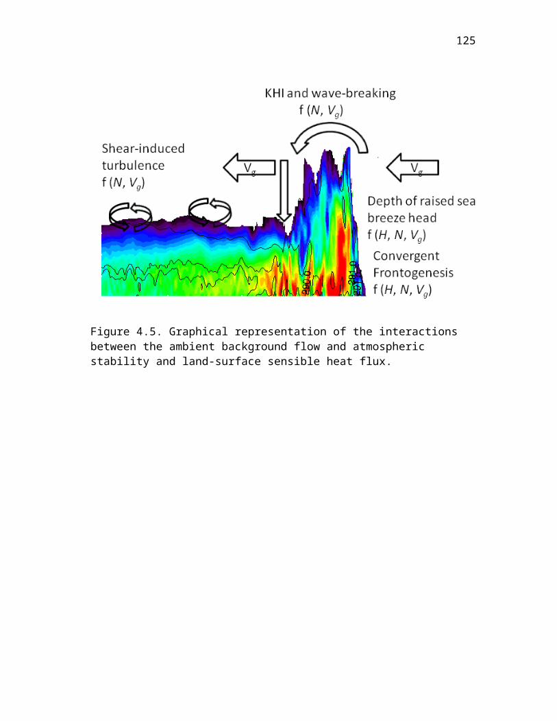
128
Liu H, Chan JCL, Cheng AYS (2001) Internal boundary layer structure under sea breeze conditions in Hong Kong. Atmos Environ 35:683-692
Lu R, Turco RP (1994) Air pollutant transport in a coastal environment. Part I: two-dimensional simulations of sea-breeze and mountain effects. J Atmos Sci 51:2285-2308
Lundquist KA, Chow FK, Lundquist JK (2010) An immersed boundary method for the Weather Research and Forecasting model. Mon Weather Rev 138:796-817
Magata M (1965) A study of the sea breeze by the numerical experiment. Pap Meteorol Geophys 16:23-36
Mahrer Y, Pielke RA (1976) Numerical simulation of the airflow over Barbados. Mon Weather Rev 104:1392–1402
Mahrer Y, Pielke RA (1977) The effects of topography on sea and land breezes in a two-dimensional numerical model. Mon Weather Rev 105:1151–1162
Mahrer Y, Segal M (1985) On the effects of islands' geometry and size on inducing sea breeze circulation. Mon Weather Rev 113:170–174
Mahrt L, Sun J, Vickers D, Macpherson JI, Pederson JR, Desjardins RL (1994) Observations of fluxes and inland breezes over a heterogeneous surface. J Atmos Sci 51:2484–2499
Mak MK, Walsh JE (1976) On the relative intensities of sea and land breezes. J Atmos Sci 33:242–251
Marshall CH, Pielke RA, Steyaert LT, Willard DA (2004) The impact of anthropogenic land-cover change on the Florida peninsula sea breezes and warm season sensible weather. Mon Weather Rev 132:28-52
Martin CL, Pielke RA (1983) The adequacy of the hydrostatic assumption in sea breeze modeling over flat terrain. J Atmos Sci 40:1472-1481
Mastrantonio G, Viola AP, Argentini S, Fiocco Giannini L, Rossini L, Abbate G, Ocone R, Casonato M (1994) Observations of sea breeze events in Rome and the surrounding area by a network of doppler sodars. Boundary-Layer Meteorol 71:67-80
McPherson RD (1970) A numerical study of the effect of a coastal irregularity on the sea breeze. J Appl Meteorol 9:767–777
129
Melas D, Kioustioukis I, Lazaridis M (2006) The impact of sea breeze on air quality in the Athens area. In: Farago L et al. (ed) Advances in air pollution modelling for environmental security, Vol 54, Springer, Netherlands, pp 285-295
Melas D, Ziomas IC, Klemm O, Zerefos CS (1998) Anatomy of the sea-breeze circulation in Athens area under weak large-scale ambient winds. Atmos Environ 32:2223-2237
Miao JF, Kroon LJM, Vila-Guerau de Arellano J, Holtslag AAM (2003) Impacts of topography and land degredation on the sea breeze over eastern Spain. Meteorol Atmos Phys 84:157-170
Millán MM, , Mantilla E, Salvador R, Carratalá A, Sanz MJ, Alonso L, Gangoiti G, Navazo M (2000) Ozone Cycles in the western Mediterranean basin: Interpretation of monitoring data in complex coastal terrain. J Appl Meteorol 39:487–508
Miller JE (1948) On the concept of frontogenesis. J Atmos Sci 5:169-171
Miller STK, Keim BD, Talbot RW, Mao H (2003) Sea breeze: structure, forecasting and impacts. Rev Geophys 41: 1/1-31
Mirocha JD, Lundquist JK, Kosović B (2010) Implementation of a nonlinear subfilter turbulence stress model for large-eddy simulation in the Advanced Research WRF model. Mon Weather Rev 138:4212-4228
Moeng CH, Dudhia J, Klemp J, Sullivan P (2007) Examining two-way grid nesting for large-eddy simulation of the PBL using the WRF model. Mon Weather Rev 135:2295-2311
Moon DA (1988) A numerical modeling investigation of the effect of convective-mesoscale interactions on the sea breeze circulation. Dissertation, University of Minnesota, Minnesota
Moroz WJ (1967) A lake breeze on the eastern shore of Lake Michigan: Observations and model. J Atmos Sci 24:337–355
Molina CA, Chen D (2009) A climatological study of the influence of synoptic flows on sea breeze evolution in the Bay of Alicante (Spain). Theor Appl Climatol 96:249-260
Neumann J (1977) On the rotation rate of the direction of sea and land breezes. J Atmos Sci 32:1913–1917
Neumann J, Mahrer Y (1971) A theoretical study of the land and sea breeze circulation. J Atmos Sci 28:532–542
130
Neumann J, Mahrer Y (1974) A theoretical study of the sea and land breezes of circular islands. J Atmos Sci 31: 2027–2039
Neumann J, Mahrer Y (1975) A theoretical study of the lake and land breezes of circular lakes. Mon Weather Rev 103:474–485
Neumann J, Savijarvi H (1986) The sea breeze on a steep coast. Beitr Phys Atmos 59:375-389
Nicholls ME, Pielke RA, Cotton WR (1991) A two-dimensional numerical investigation of the interaction between sea breezes and deep convection over the Florida Peninsula. Mon Weather Rev 119: 298-323
Niino H (1987) The linear theory of land, and sea breeze circulation. J Meteorol Soc Jpn 65: 901-920
Noonan JA, Smith RK (1986) Sea-breeze circulations over Cape York Peninsula and the generation of Gulf of Carpentaria cloud line disturbances. J Atmos Sci 43:1679-1693
Novak DR, Colle BA (2006) Observations of multiple sea breeze boundaries during an unseasonably warm day in metropolitan New York City. Bull Am Meteorol Soc 87:169-174
Ogawa S, Sha W, Iwasaki T (2003) A numerical study of the interaction of a sea-breeze front with convective cells in the daytime boundary layer. J Meteorol Soc Jpn 81: 635-651
Ohashi Y, Kida H (2002) Local circulations developed in the vicinity of both coastal and inland urban areas: A numerical study with a mesoscale atmospheric model. J Appl Meteorol 41:30-45
Ohashi Y, Kida H (2004) Local circulations developed in the vicinity of both coastal and inland urban areas. Part II: effects of urban and mountain areas on moisture transport. J Appl Meteorol 43:119-133
Ookouchi Y, Uryu M, Sawada R (1978) A numerical study of the effects of a mountain on the land and sea breeze. J Meteorol Soc Jpn 56:368-386
Ookouchi Y, Segal M, Kessler RC, Pielke RA (1984) Evaluation of soil moisture on the generation and modification of mesoscale circulation. Mon Weather Rev 112:2281-2292
Pearson RA (1973) Properties of the sea breeze front as shown by a numerical model. J Atmos Sci 30:1050-1060
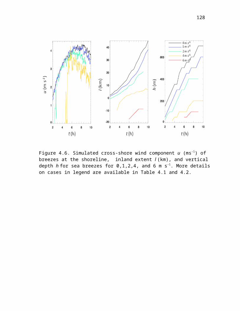
131
Pearson RA, Carboni G, Brusasca G (1983) The sea breeze with mean flow. Q J Roy Meteorol Soc 109: 809–830
Pearce RP (1955) The calculation a sea breeze circulation in terms of the differential heating across the coastline. Q J Roy Meteorol Soc 81:351-381
Porson A, Steyn DG, Schayes G (2007a) Sea breeze scaling from numerical model simulations. Part 1: pure sea breezes. Boundary-Layer Meteorol 122:17-29
Porson A, Steyn DG, Schayes G (2007b) Sea breeze scaling from numerical model simulations. Part II: interactions between the sea breeze and slope flows. Boundary-Layer Meteorol 122:31-41
Porson A, Steyn DG, Schayes G (2007c) Formulation of an index for sea breezes in opposing winds. J Clim Appl Meteorol 46:1257-1263
Physick WL (1976) A numerical model of the sea breeze phenomenon over a lake or gulf. J Atmos Sci 33:2107-2135
Physick WL (1980) Numerical experiments on the inland penetration of the sea breeze. Q J Roy Meteorol Soc 106:735–746
Physick WL, Smith RK (1985) Observations and dynamics of sea-breezes in northern Australia. Aust Meteorol Mag 33:51-63
Pielke RA (1974a) A three-dimensional numerical model of the sea breezes over South Florida. Mon Weather Rev 102:115–139
Pielke RA (1974b) A comparison of three-dimensional and two-dimensional numerical prediction of sea breezes. J Atmos Sci 31:1577-1585
Pielke RA, Segal M (1986) Mesoscale circulations forced by differential terrain heating. In PS Ray (ed), Mesoscale meteorology and forecasting, Amer Meteorol Soc, Boston, pp 516-548
Plant RS, Keith GJ (2007) Occurrence of Kelvin-Helmholtz billows in sea breeze circulations. Boundary-Layer Meteorol 122:1-15
Puygrenier V, Lohou F, Campistron B, Said F, Pigeon G, Benech B, Serca D (2005) Investigation on the fine structure of sea-breeze during ESCOMPTE experiment. Atmos Res 74: 329-353
Qian T, Epifanio CC, Zhang F (2009) Linear theory calculations for the sea breeze in a background wind: The equatorial case. J Atmos Sci 66:1749-1763
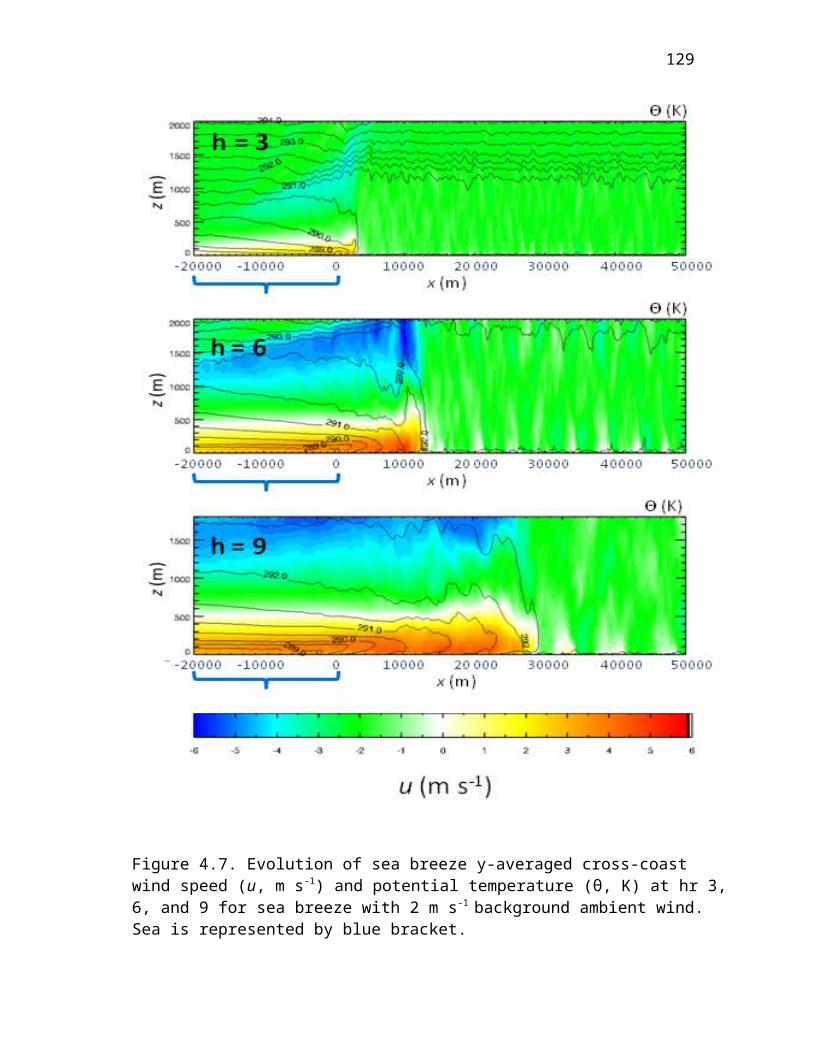
132
Ramis C, Romero R (1995) A first numerical simulation of the development and structure of the sea breeze in the island of Mallorca. Ann Geophys 13:981-994
Rao PN, Fuelberg HE (2000) An Investigation of convection behind the Cape Canaveral sea- breeze front. Mon Weather Rev 128:3437-3458
Rao PN, Fuelberg HE, Droegemeier KK (1999) High-resolution modeling of the Cape Canaveral area land-water circulations and associated features. Mon Weather Rev 127:1808-1821
Richiardone R, Pearson RA (1983) Inland convection and energy transfers in a sea breeze model. Q J Roy Meteorol Soc 109:325-338
Ries H, Schlunzen KH (2009) Evaluation of a mesoscale model with different surface parameterizations and vertical resolutions for the bay of Valencia. Mon Weather Rev 137:2646-2661
Rotunno R, Chen Y, Wang W, Davis CA, Dudhia J, Holland GJ (2009) Large-eddy simulation of an idealized tropical cyclone. Bull Am Meteorol Soc 90:1783-1788
Rotunno R (1983) On the linear theory of the land and sea breeze. J Atmos Sci 40:1999–2009
Samuelsson P, Tjernstrom M (2001) Mesoscale flow modification induced by land-lake surface temperature and roughness differences. J Geophys Res 106:12419-12435
Savijarvi H (1997) Diurnal winds around Lake Tanganyika. Q J Roy Meteorol Soc 123:901-918
Savijarvi H, Alestalo M (1988) The sea breeze over a lake or gulf as the function of the prevailing flow. Beitr Phys Atmos 61:98-104
Savijarvi H, Matthews S (2004) Flow over small heat islands: A numerical sensitivity study. J Atmos Sci 61: 859–868
Schlunzen KH (1990) Numerical studies on the inland penetration of sea breeze fronts at a coastline with tidally flooded mudflats. Beitr Phys Atmos 63:243-256
Segal M, Pielke RA (1985) On the effect of water temperature and synoptic flows on the development of surface flows over narrow-elongated water bodies. J Geophys Res 90:4907–4910
Segal M, Arritt R (1992) Nonclassical mesoscale circulations caused by surface sensible heat-flux gradients. Bull Am Meteorol Soc 73:1593–1604
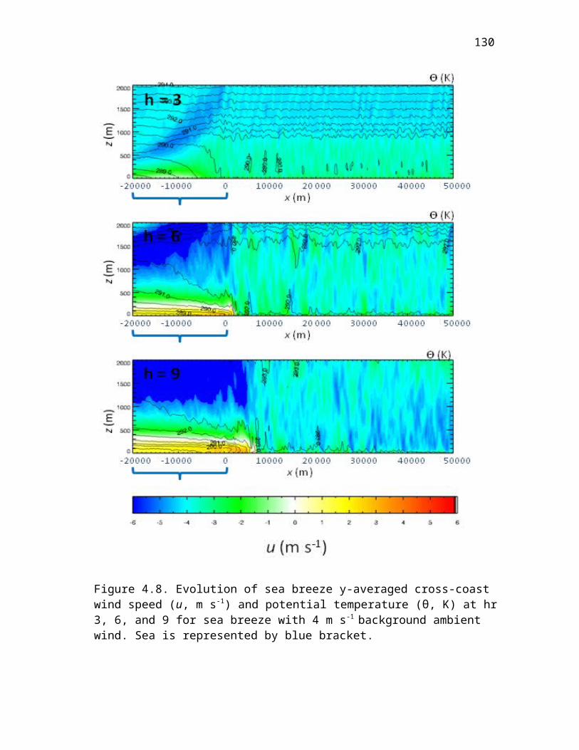
133
Segal M, Mahrer Y, Pielke RA (1983) A study of meteorological patterns associated with a lake confined by mountains -- the Dead Sea case. Q J Roy Meteorol Soc 109:549–564
Segal M, Avissar R, McCumber M, Pielke R (1988) Evaluation of vegetation effects on the generation and modification of mesoscale circulations. J Atmos Sci 45:2268–2293
Segal M, Purdom J, Song J, Pielke R, Mahrer Y (1986) Evaluation of cloud shading effects on the generation and modification of mesoscale circulations. Mon Weather Rev 114:1201-1212
Segal M, Leuthold M, Arritt RW, Anderson C, Shen J (1997) Small lake daytime breezes: Some observational and conceptual evaluations. Bull Am Meteorol Soc 78:1135–1147
Sha W, Kawamura T, Ueda H (1991) A numerical study on sea/land breezes as a gravity current: Kelvin–Helmholtz billows and inland penetration of the sea-breeze front. J Atmos Sci 48:1649–1665
Sha W, Kawamura T, Ueda H (1993) A numerical study of nocturnal sea/land breezes: Prefrontal gravity waves in the compensating flow and inland penetration of the sea-breeze cutoff vortex. J Atmos Sci 50:1076-1088
Sha W, Ogawa S, Iwasaki T (2004) A numerical study on the nocturnal frontogenesis of the sea breeze front. J Meteorol Soc Jpn 82:817-823
Shaw W, Lundquist JK, Schreck S (2009) Research needs for wind resource characterization. Bull Am Meteorol Soc 90:535-538
Sheih CM, Moroz WJ (1975) Mathematical modelling of lake breeze. Atmos Environ 9:575-586
Shen J (1998) Numerical Modelling of the effects of vegetation and environmental conditions on the lake breeze. Boundary-Layer Meteorol 87:481-498
Shepherd JM, Ferrier BS, Ray PS (2001) Rainfall morphology in Florida convergence zones: A numerical study. Mon Weather Rev 129:177-197
Simpson JE (1994) Sea breeze and local winds. Cambridge University Press, UK, 234 pp
Simpson JE (1997) Gravity currents: In the environment and in the laboratory. Vol 4. Cambridge University Press, UK, 244 pp
Simpson JE, Mansfield DA, Milford JR (1977) Inland penetration of sea-breeze fronts. Q J Roy Meteorol Soc 103:47-76
134
Skamarock WC, Klemp JB (2008) A time-split nonhydrostatic atmospheric model for weather research and forecasting applications. J Comp Phys 227:3465-3485
Skamarock WC, Klemp JB, Dudhia J, Gill DO, Barker DM, Duda MG, Huang X-Y, Wang W, Powers JG (2008) A description of the advanced research WRF version 3. NCAR/TN-475, 113 pp
Small E, Giorgi F, Sloan L, Hostetler S (2001) The effects of dessication and climate change on the hydrology of the Aral Sea. J Clim 14:300-222
Song JL (1986) A numerical investigation of Florida’s sea breeze-cumulonimbus interactions. Dissertation, Colorado State University, Colorado
Srinivas CV, Venkatesan R, Singh A (2007) Sensitivity of mesoscale simulations of land-sea breeze to boundary layer turbulence parameterization. Atmos Environ 41:2534-2548
Stephan K, Kraus H, Ewenz CM, Hacker JM (1999) Sea-breeze front variations in space and time. Meteorol Atmos Phys 70:81-95
Stivari SMS, de Oliveira AP, Karam HA, Soares J (2003) Patterns of local circulation in the Itaipu Lake area: Numerical simulations of lake breeze. J Appl Meteorol 42:37-50
Steyn DG, (1998) Scaling the vertical structure of sea breezes. Boundary-Layer Meteorol 86:505-524
Steyn DG (2003) Scaling the vertical structure of sea breezes revisited. Boundary-Layer Meteorol 107:177-188
Steyn DG, Mckendry I (1988) Quantitative and qualitative evaluation of a three-dimensional mesoscale numerical model simulation of a sea breeze in complex terrain. Mon Weather Rev 116:1914–1926
Steyn DG, Kallos G (1992) A study of the dynamics of hodograph rotation in the sea breezes of Attica, Greece. Boundary-Layer Meteorol 58:215-228
Sun J, Lenschow D, Mahrt L, Crawford TL, Davis K, Oncley SP, MacPherson JI, Wang Q, Dobosy RJ, Desjardins RL (1997) Lake-induced atmospheric circulations during BOREAS. J Geophys Res 102: 29155-29166
Talbot C, Augustin P, Leroy C, Willart V, Delbarre H, Khomenko G (2007) Impact of a sea breeze on the boundary-layer dynamics and the atmospheric stratification in a coastal area of the North Sea. Boundary-Layer Meteorol 125:133-154
135
Thompson WT, Holt T, Pullen J (2007) Investigation of a sea breeze front in an urban environment. Q J Roy Meteorol Soc 133:579-594
Tijm ABC, Van Delden AJ (1999) The role of sound waves in sea-breeze initiation. Q J Roy Meteorol Soc 125:1997-2018
Tijm ABC, Holtslag AAM, Van Delden AJ (1999a) Observations and modeling of the sea breeze with the return current. Mon Weather Rev 127:625–640
Tijm ABC, Van Delden AJ, Holtslag AAM (1999b) The inland penetration of sea breezes. Contrib Atmos Phys 72: 317-328
Troen, I (1982) Analytical and numerical modelling of flow driven by surface differential heating. Dissertation, University of Copenhagen, Denmark
Wakimoto RM, Atkins NT (1994) Observations of the sea-breeze front during CaPE. Part I: single-doppler, satellite, and cloud photogrammetry analysis. Mon Weather Rev 122:1092-1114
Walsh JE (1974) Sea breeze theory and applications. J Atmos Sci 31:2012–2026 Wang J, Eltahir EAB, Bras RL (1998) Numerical simulation of nonlinear mesoscale
circulations induced by the thermal heterogeneities of land surface. J Atmos Sci 55:447–464
Wood R, Stromberg IM, Jonas PR (1999) Aircraft observations of sea breeze frontal structure. Q J Roy Meteorol Soc 125:1959-1995
Yan H, Anthes RA (1987) The effect of latitude on the sea breeze. Mon Weather Rev 115:936–956
Yan H, Anthes RA (1988) The effect of variations in surface moisture on mesoscale circulation. Mon Weather Rev 116:192–208
Yang X (1991) A study of nonhydrostatic effects in idealized sea breeze systems. Boundary-Layer Meteorol 54:183-208
Yimin M, Lyons TJ (2000) Numerical simulations of a sea breeze under dominant synoptic conditions at Perth. Meteorol Atmos Phys 73:89-103
Yoshikado H (1990) Vertical structure of the sea breeze penetrating through a large urban complex. J Appl Meteorol 29:878-891
Yoshikado H (1992) Numerical study of the daytime urban effect and its interaction with the sea breeze. J Appl Meteorol 31:1146-1164
Xian Z, Pielke RA (1991) The effects of width of land masses on the development of sea breezes. J Appl Meteorol 30:1280-1304
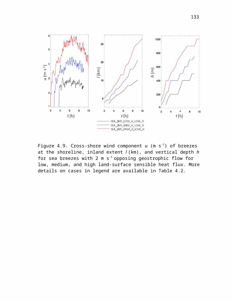
136
Zhang Y, Chen YL, Schroeder TA (2005) Numerical simulations of sea breeze circulations over Northwest Hawaii Weather Forecast 20:827-846
Zhong S, Takle ES (1993) The Effects of large-scale winds on the sea-land-breeze circulations in an area of complex coastal heating. J Appl Meteorol 32:1181–1195
Zhong S, Leone JM, Tackle ES (1991) Interaction of the sea breeze with a river breeze in an area of complex coastal heating. Boundary-Layer Meteorol 56:101-139
Zhu M, Atkinson BW (2004) Observed and modelled climatology of the land-sea breeze circulation over the Persian Gulf. Int J Climatol 24:883-905.
![[PPT]Numerical Differentiation and Integration Part 6 · Web viewNumerical Differentiation and Integration Standing in the heart of calculus are the mathematical concepts of differentiation](https://img.pdfslide.us/doc/110x75/5ae57d5b7f8b9aee078b9dea/pptnumerical-differentiation-and-integration-part-6-viewnumerical-differentiation.jpg)