Dra

ft

1

History of Random Number Generators

Seed x0,xi = f (xi−1),ui = g(xi)

Pierre L’Ecuyer

December 9, 2017

Dra

ft

2

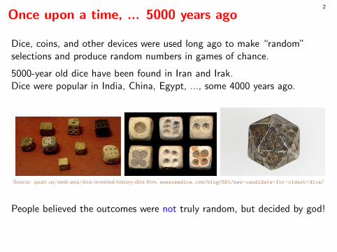
Once upon a time, ... 5000 years ago

Dice, coins, and other devices were used long ago to make “random”selections and produce random numbers in games of chance.

5000-year old dice have been found in Iran and Irak.Dice were popular in India, China, Egypt, ..., some 4000 years ago.

Source: quatr.us/west-asia/dice-invented-history-dice.htm, awesomedice.com/blog/551/new-candidate-for-oldest-dice/

People believed the outcomes were not truly random, but decided by god!

Dra

ft

3

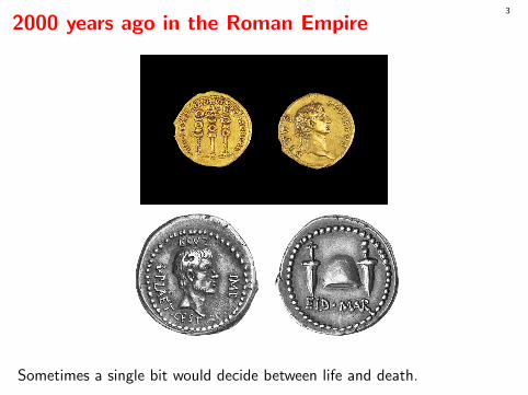
2000 years ago in the Roman Empire

Sometimes a single bit would decide between life and death.

Dra

ft

4

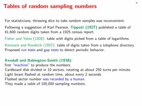
Tables of random sampling numbers

For statisticians, throwing dice to take random samples was inconvenient.

Following a suggestion of Karl Pearson, Tippett (1927) published a table of41,600 random digits taken from a 1925 census report.

Fisher and Yates (1928): table with digits picked from a table of logarithms.

Kermack and Kendrick (1937): table of digits taken from a telephone directory.Proposed run tests and gap tests to detect periodic behavior.

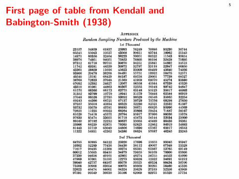
Kendall and Babington-Smith (1938):first “machine” to produce the numbers.Cardboard disk divided in 10 sectors, rotating at about 250 turns per minute.Light beam flashed at random time, about every 2 seconds.Flashed sector number was recorded by a human.They made a table of 100,000 sampling numbers.

Dra

ft

5

First page of table from Kendall andBabington-Smith (1938)

Dra

ft

6

How to measure the quality of a table?

Probability theory: for independent random digits, any possible table of ndigits has the same probability, so no table is better than another!

KBS introduced a notion of locally random sequence: every reasonablylong subsequence should appear random and pass simple statistical tests.

They proposed a small set of tests that measure:(1) the frequency of each digit;(2) the frequency of each pair in successive values (serial test);(3) the frequency of certain blocks of five digits (poker);(4) lengths of gaps between the occurrences of a given digit.Frequencies are compared with expectations via a chi-square.

They replicated the tests with disjoint parts of their table.Their table passed the tests.

Dra

ft

6

How to measure the quality of a table?

Probability theory: for independent random digits, any possible table of ndigits has the same probability, so no table is better than another!

KBS introduced a notion of locally random sequence: every reasonablylong subsequence should appear random and pass simple statistical tests.

They proposed a small set of tests that measure:(1) the frequency of each digit;(2) the frequency of each pair in successive values (serial test);(3) the frequency of certain blocks of five digits (poker);(4) lengths of gaps between the occurrences of a given digit.Frequencies are compared with expectations via a chi-square.

They replicated the tests with disjoint parts of their table.Their table passed the tests.

Dra

ft

7

1947: RAND Corporation projectof a million random digits

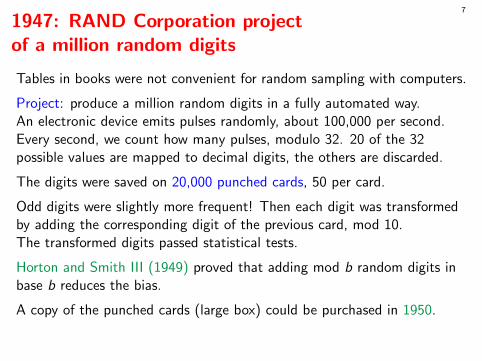
Tables in books were not convenient for random sampling with computers.

Project: produce a million random digits in a fully automated way.An electronic device emits pulses randomly, about 100,000 per second.Every second, we count how many pulses, modulo 32. 20 of the 32possible values are mapped to decimal digits, the others are discarded.

The digits were saved on 20,000 punched cards, 50 per card.

Odd digits were slightly more frequent! Then each digit was transformedby adding the corresponding digit of the previous card, mod 10.The transformed digits passed statistical tests.

Horton and Smith III (1949) proved that adding mod b random digits inbase b reduces the bias.

A copy of the punched cards (large box) could be purchased in 1950.

Dra

ft

7

1947: RAND Corporation projectof a million random digits

Tables in books were not convenient for random sampling with computers.

Project: produce a million random digits in a fully automated way.An electronic device emits pulses randomly, about 100,000 per second.Every second, we count how many pulses, modulo 32. 20 of the 32possible values are mapped to decimal digits, the others are discarded.

The digits were saved on 20,000 punched cards, 50 per card.

Odd digits were slightly more frequent! Then each digit was transformedby adding the corresponding digit of the previous card, mod 10.The transformed digits passed statistical tests.

Horton and Smith III (1949) proved that adding mod b random digits inbase b reduces the bias.

A copy of the punched cards (large box) could be purchased in 1950.

Dra

ft

8

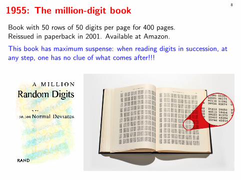
1955: The million-digit book

Book with 50 rows of 50 digits per page for 400 pages.Reissued in paperback in 2001. Available at Amazon.

This book has maximum suspense: when reading digits in succession, atany step, one has no clue of what comes after!!!

Dra

ft

9

Generating random numbers on the fly

For physicists doing Monte Carlo simulation, reading random digits frompunched cards or tables was too slow and memory was also limited.

Two main approaches:1. A fast physical device (electronic noise, etc.);2. A purely deterministic algorithm that imitates randomness in software.

At the end of the RAND report of Brown (1949):“... for the future ... it may not be asking too much to hope that ... somenumerical process will permit us to produce our random numbers as weneed them. The advantages of such a method are fairly obvious inlarge-scale computation where extensive tabling operations are relativelyclumsy.”

Dra

ft

10

Physical devices

Coins, dice, roulette, picking balls from an urn, shuffling cards, etc., havebeen used for centuries.

With computers, electronic devices such as counters of random events andperiodic sampling of electric noise, are faster and more convenient.

Thousands of articles and around 2000 patents for physical RNGs in thelast 70 years! Thermal and electric noise, photoelectric effect, devicesbased on quantum physics phenomena such as light beam splitters, shotnoise in electronic circuits, radioactive decay detected by a Geigercounter, etc.

An early example: Cobine and Curry (1947): electric noise in a gas tubein a magnetic field is amplified and sampled to produce random bits.

Transformation techniques to reduce biais and correlations.

Fastest commercial devices today produce about 3 Gbits per second.

Dra

ft

11

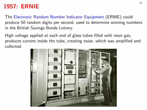
1957: ERNIE

The Electronic Random Number Indicator Equipment (ERNIE) couldproduce 50 random digits per second, used to determine winning numbersin the British Savings Bonds Lottery.

High voltage applied at each end of glass tubes filled with neon gas,produces current inside the tube, creating noise, which was amplified andcollected.

Dra

ft

12

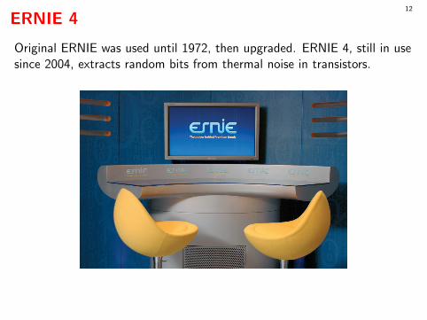
ERNIE 4

Original ERNIE was used until 1972, then upgraded. ERNIE 4, still in usesince 2004, extracts random bits from thermal noise in transistors.

Dra

ft

13

Our ERNIE, 2017

Dra

ft

14

Our ERNIE, 2017

Dra

ft

15

Algorithmic generators

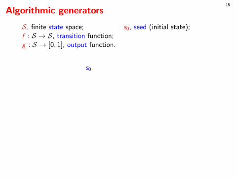
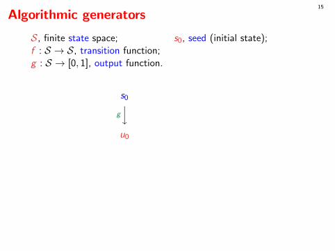
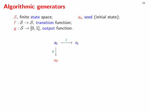
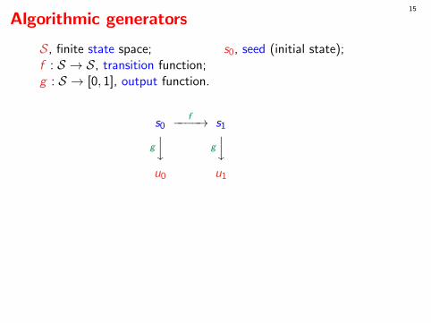
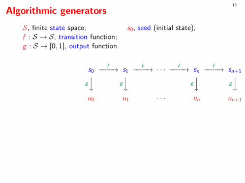
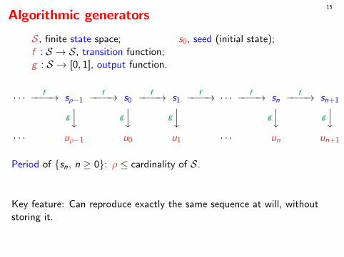
S, finite state space; s0, seed (initial state);f : S → S, transition function;g : S → [0, 1], output function.

· · · f−−−−→ sρ−1f−−−−→

s0

f−−−−→ s1f−−−−→ · · · f−−−−→ sn

f−−−−→ sn+1f−−−−→ · · ·

g

y g

y g

y g

y g

y· · · uρ−1 u0 u1 · · · un un+1 · · ·

Period of {sn, n ≥ 0}: ρ ≤ cardinality of S.

Key feature: Can reproduce exactly the same sequence at will, withoutstoring it.

Dra

ft

15

Algorithmic generators

S, finite state space; s0, seed (initial state);f : S → S, transition function;g : S → [0, 1], output function.

· · · f−−−−→ sρ−1f−−−−→

s0

f−−−−→ s1f−−−−→ · · · f−−−−→ sn

f−−−−→ sn+1f−−−−→ · · ·

g

y

g

y

g

y g

y g

y· · · uρ−1

u0

u1 · · · un un+1 · · ·

Period of {sn, n ≥ 0}: ρ ≤ cardinality of S.

Key feature: Can reproduce exactly the same sequence at will, withoutstoring it.

Dra

ft

15

Algorithmic generators

S, finite state space; s0, seed (initial state);f : S → S, transition function;g : S → [0, 1], output function.

· · · f−−−−→ sρ−1f−−−−→

s0f−−−−→ s1

f−−−−→ · · · f−−−−→ snf−−−−→ sn+1

f−−−−→ · · ·

g

y

g

y

g

y g

y g

y· · · uρ−1

u0

u1 · · · un un+1 · · ·

Period of {sn, n ≥ 0}: ρ ≤ cardinality of S.

Key feature: Can reproduce exactly the same sequence at will, withoutstoring it.

Dra

ft

15

Algorithmic generators

S, finite state space; s0, seed (initial state);f : S → S, transition function;g : S → [0, 1], output function.

· · · f−−−−→ sρ−1f−−−−→

s0f−−−−→ s1

f−−−−→ · · · f−−−−→ snf−−−−→ sn+1

f−−−−→ · · ·

g

y

g

y g

y

g

y g

y· · · uρ−1

u0 u1

· · · un un+1 · · ·

Period of {sn, n ≥ 0}: ρ ≤ cardinality of S.

Key feature: Can reproduce exactly the same sequence at will, withoutstoring it.

Dra

ft

15

Algorithmic generators

S, finite state space; s0, seed (initial state);f : S → S, transition function;g : S → [0, 1], output function.

· · · f−−−−→ sρ−1f−−−−→

s0f−−−−→ s1

f−−−−→ · · · f−−−−→ snf−−−−→ sn+1

f−−−−→ · · ·

g

y

g

y g

y g

y g

y

· · · uρ−1

u0 u1 · · · un un+1 · · ·

Period of {sn, n ≥ 0}: ρ ≤ cardinality of S.

Key feature: Can reproduce exactly the same sequence at will, withoutstoring it.

Dra

ft

15

Algorithmic generators

S, finite state space; s0, seed (initial state);f : S → S, transition function;g : S → [0, 1], output function.

· · · f−−−−→ sρ−1f−−−−→ s0

f−−−−→ s1f−−−−→ · · · f−−−−→ sn

f−−−−→ sn+1f−−−−→ · · ·

g

y g

y g

y g

y g

y· · · uρ−1 u0 u1 · · · un un+1 · · ·

Period of {sn, n ≥ 0}: ρ ≤ cardinality of S.

Key feature: Can reproduce exactly the same sequence at will, withoutstoring it.

Dra

ft

16

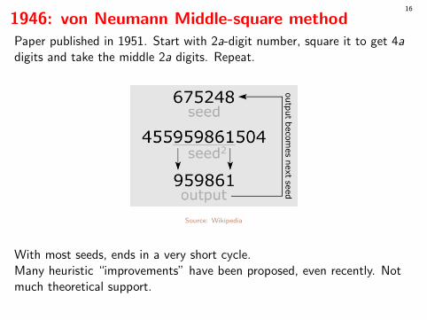
1946: von Neumann Middle-square methodPaper published in 1951. Start with 2a-digit number, square it to get 4adigits and take the middle 2a digits. Repeat.

Source: Wikipedia

With most seeds, ends in a very short cycle.Many heuristic “improvements” have been proposed, even recently. Notmuch theoretical support.

Dra

ft

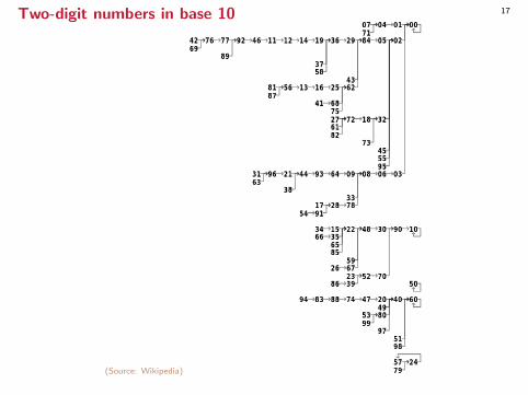
17Two-digit numbers in base 10

(Source: Wikipedia)

Dra

ft

18

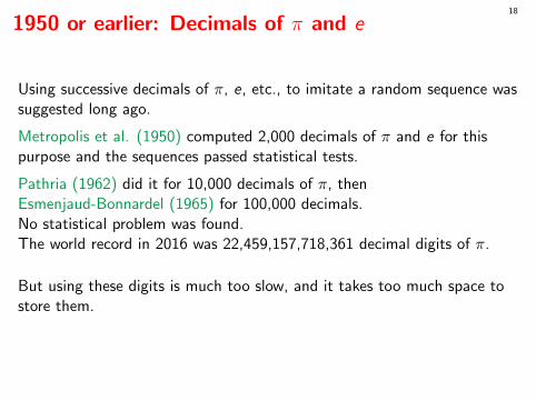
1950 or earlier: Decimals of π and e

Using successive decimals of π, e, etc., to imitate a random sequence wassuggested long ago.

Metropolis et al. (1950) computed 2,000 decimals of π and e for thispurpose and the sequences passed statistical tests.

Pathria (1962) did it for 10,000 decimals of π, thenEsmenjaud-Bonnardel (1965) for 100,000 decimals.No statistical problem was found.The world record in 2016 was 22,459,157,718,361 decimal digits of π.

But using these digits is much too slow, and it takes too much space tostore them.

Dra

ft

19

Notions of uniformly distributed infinite sequence

A more fundamental question: what can we prove about the uniformityand independence of these successive digits, in the long run?

Borel (1909): A sequence of digits in base b is k-distributed if any of thebk possible blocks of k successive digits appears with the same frequencyin the long run. It is ∞-distributed if this holds for any k ≥ 1.

Borel proved that almost all real numbers (w.r.t. uniform measure) havean ∞-distributed digital expansion in base b for any b (i.e., they arenormal numbers). We do not know if π or e is a normal number.

Similar notions of uniformity for sequences of real numbers in [0, 1) werestudied by Weyl (1916), Korobov (1948), Franklin (1963, 1965), etc. SeeKuipers and Niederreiter (1974).

Sequences that provably satisfy these definitions can be constructed, butthey are impractical for simulation, and often do not look random.

Dra

ft

19

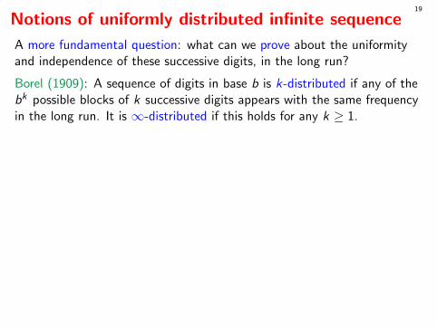
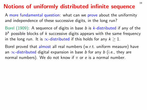
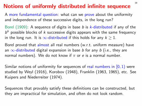
Notions of uniformly distributed infinite sequence

A more fundamental question: what can we prove about the uniformityand independence of these successive digits, in the long run?

Borel (1909): A sequence of digits in base b is k-distributed if any of thebk possible blocks of k successive digits appears with the same frequencyin the long run. It is ∞-distributed if this holds for any k ≥ 1.

Borel proved that almost all real numbers (w.r.t. uniform measure) havean ∞-distributed digital expansion in base b for any b (i.e., they arenormal numbers). We do not know if π or e is a normal number.

Similar notions of uniformity for sequences of real numbers in [0, 1) werestudied by Weyl (1916), Korobov (1948), Franklin (1963, 1965), etc. SeeKuipers and Niederreiter (1974).

Sequences that provably satisfy these definitions can be constructed, butthey are impractical for simulation, and often do not look random.

Dra

ft

19

Notions of uniformly distributed infinite sequence

A more fundamental question: what can we prove about the uniformityand independence of these successive digits, in the long run?

Borel (1909): A sequence of digits in base b is k-distributed if any of thebk possible blocks of k successive digits appears with the same frequencyin the long run. It is ∞-distributed if this holds for any k ≥ 1.

Borel proved that almost all real numbers (w.r.t. uniform measure) havean ∞-distributed digital expansion in base b for any b (i.e., they arenormal numbers). We do not know if π or e is a normal number.

Similar notions of uniformity for sequences of real numbers in [0, 1) werestudied by Weyl (1916), Korobov (1948), Franklin (1963, 1965), etc. SeeKuipers and Niederreiter (1974).

Sequences that provably satisfy these definitions can be constructed, butthey are impractical for simulation, and often do not look random.

Dra

ft

20

RNGs with long known finite period

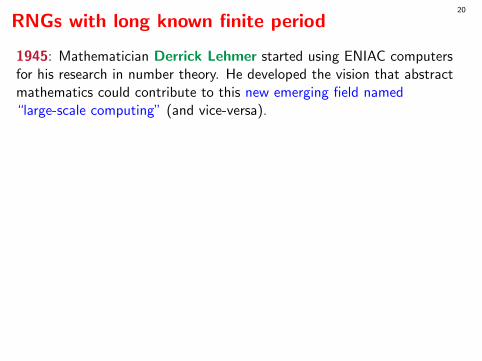
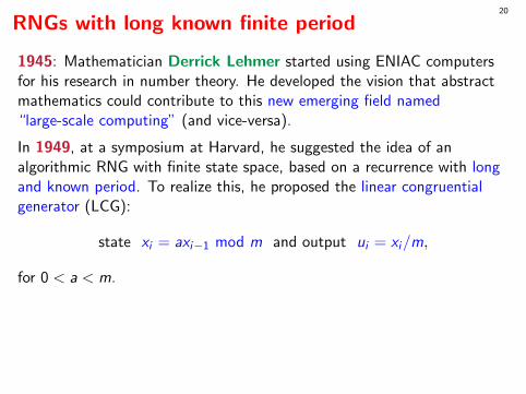
1945: Mathematician Derrick Lehmer started using ENIAC computersfor his research in number theory. He developed the vision that abstractmathematics could contribute to this new emerging field named“large-scale computing” (and vice-versa).

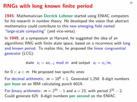
In 1949, at a symposium at Harvard, he suggested the idea of analgorithmic RNG with finite state space, based on a recurrence with longand known period. To realize this, he proposed the linear congruentialgenerator (LCG):

state xi = axi−1 mod m and output ui = xi/m,

for 0 < a < m. He proposed two specific ones:

For decimal arithmetic: m = 108 + 1. Generated 1,250 8-digit numbersper hour on an IBM calculating punch 602A.

For binary arithmetic: m = 231 − 1 and a = 23, with period 231 − 2.Could generate 625 8-digit numbers per second on the ENIAC.

Dra

ft

20

RNGs with long known finite period

1945: Mathematician Derrick Lehmer started using ENIAC computersfor his research in number theory. He developed the vision that abstractmathematics could contribute to this new emerging field named“large-scale computing” (and vice-versa).

In 1949, at a symposium at Harvard, he suggested the idea of analgorithmic RNG with finite state space, based on a recurrence with longand known period. To realize this, he proposed the linear congruentialgenerator (LCG):

state xi = axi−1 mod m and output ui = xi/m,

for 0 < a < m.

He proposed two specific ones:

For decimal arithmetic: m = 108 + 1. Generated 1,250 8-digit numbersper hour on an IBM calculating punch 602A.

For binary arithmetic: m = 231 − 1 and a = 23, with period 231 − 2.Could generate 625 8-digit numbers per second on the ENIAC.

Dra

ft

20

RNGs with long known finite period

1945: Mathematician Derrick Lehmer started using ENIAC computersfor his research in number theory. He developed the vision that abstractmathematics could contribute to this new emerging field named“large-scale computing” (and vice-versa).

In 1949, at a symposium at Harvard, he suggested the idea of analgorithmic RNG with finite state space, based on a recurrence with longand known period. To realize this, he proposed the linear congruentialgenerator (LCG):

state xi = axi−1 mod m and output ui = xi/m,

for 0 < a < m. He proposed two specific ones:

For decimal arithmetic: m = 108 + 1. Generated 1,250 8-digit numbersper hour on an IBM calculating punch 602A.

For binary arithmetic: m = 231 − 1 and a = 23, with period 231 − 2.Could generate 625 8-digit numbers per second on the ENIAC.

Dra

ft

21

Many more LCGs

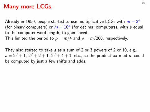
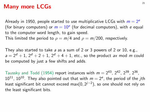
Already in 1950, people started to use multiplicative LCGs with m = 2e

(for binary computers) or m = 10e (for decimal computers), with e equalto the computer word length, to gain speed.This limited the period to ρ = m/4 and ρ = m/200, respectively.

They also started to take a as a sum of 2 or 3 powers of 2 or 10, e.g.,a = 2d + 1, 2d + 2 + 1, 2d + 4 + 1, etc., so the product ax mod m couldbe computed by just a few shifts and adds.

Taussky and Todd (1954) report instances with m = 243, 242, 239, 236,1011, 1010. They also pointed out that with m = 2e , the period of the jthleast significant bit cannot exceed max(0, 2j−2), so one should not rely onthe least significant bits.

Dra

ft

21

Many more LCGs

Already in 1950, people started to use multiplicative LCGs with m = 2e

(for binary computers) or m = 10e (for decimal computers), with e equalto the computer word length, to gain speed.This limited the period to ρ = m/4 and ρ = m/200, respectively.

They also started to take a as a sum of 2 or 3 powers of 2 or 10, e.g.,a = 2d + 1, 2d + 2 + 1, 2d + 4 + 1, etc., so the product ax mod m couldbe computed by just a few shifts and adds.

Taussky and Todd (1954) report instances with m = 243, 242, 239, 236,1011, 1010. They also pointed out that with m = 2e , the period of the jthleast significant bit cannot exceed max(0, 2j−2), so one should not rely onthe least significant bits.

Dra

ft

22

Adding a constant term

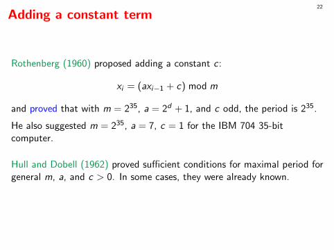
Rothenberg (1960) proposed adding a constant c :

xi = (axi−1 + c) mod m

and proved that with m = 235, a = 2d + 1, and c odd, the period is 235.

He also suggested m = 235, a = 7, c = 1 for the IBM 704 35-bitcomputer.

Hull and Dobell (1962) proved sufficient conditions for maximal period forgeneral m, a, and c > 0. In some cases, they were already known.

Dra

ft

23

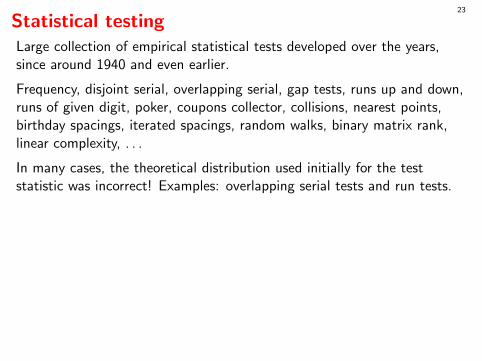
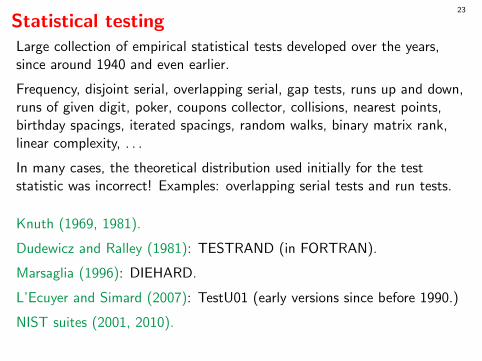
Statistical testingLarge collection of empirical statistical tests developed over the years,since around 1940 and even earlier.

Frequency, disjoint serial, overlapping serial, gap tests, runs up and down,runs of given digit, poker, coupons collector, collisions, nearest points,birthday spacings, iterated spacings, random walks, binary matrix rank,linear complexity, . . .

In many cases, the theoretical distribution used initially for the teststatistic was incorrect! Examples: overlapping serial tests and run tests.

Knuth (1969, 1981).

Dudewicz and Ralley (1981): TESTRAND (in FORTRAN).

Marsaglia (1996): DIEHARD.

L’Ecuyer and Simard (2007): TestU01 (early versions since before 1990.)

NIST suites (2001, 2010).

Dra

ft

23

Statistical testingLarge collection of empirical statistical tests developed over the years,since around 1940 and even earlier.

Frequency, disjoint serial, overlapping serial, gap tests, runs up and down,runs of given digit, poker, coupons collector, collisions, nearest points,birthday spacings, iterated spacings, random walks, binary matrix rank,linear complexity, . . .

In many cases, the theoretical distribution used initially for the teststatistic was incorrect! Examples: overlapping serial tests and run tests.

Knuth (1969, 1981).

Dudewicz and Ralley (1981): TESTRAND (in FORTRAN).

Marsaglia (1996): DIEHARD.

L’Ecuyer and Simard (2007): TestU01 (early versions since before 1990.)

NIST suites (2001, 2010).

Dra

ft

24

The spectral test

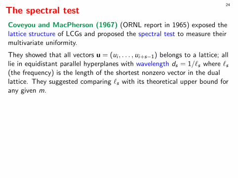
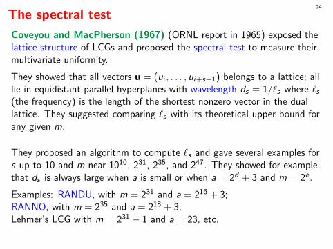
Coveyou and MacPherson (1967) (ORNL report in 1965) exposed thelattice structure of LCGs and proposed the spectral test to measure theirmultivariate uniformity.

They showed that all vectors u = (ui , . . . , ui+s−1) belongs to a lattice; alllie in equidistant parallel hyperplanes with wavelength ds = 1/`s where `s(the frequency) is the length of the shortest nonzero vector in the duallattice. They suggested comparing `s with its theoretical upper bound forany given m.

They proposed an algorithm to compute `s and gave several examples fors up to 10 and m near 1010, 231, 235, and 247. They showed for examplethat ds is always large when a is small or when a = 2d + 3 and m = 2e .

Examples: RANDU, with m = 231 and a = 216 + 3;RANNO, with m = 235 and a = 218 + 3;Lehmer’s LCG with m = 231 − 1 and a = 23, etc.

Dra

ft

24

The spectral test

Coveyou and MacPherson (1967) (ORNL report in 1965) exposed thelattice structure of LCGs and proposed the spectral test to measure theirmultivariate uniformity.

They showed that all vectors u = (ui , . . . , ui+s−1) belongs to a lattice; alllie in equidistant parallel hyperplanes with wavelength ds = 1/`s where `s(the frequency) is the length of the shortest nonzero vector in the duallattice. They suggested comparing `s with its theoretical upper bound forany given m.

They proposed an algorithm to compute `s and gave several examples fors up to 10 and m near 1010, 231, 235, and 247. They showed for examplethat ds is always large when a is small or when a = 2d + 3 and m = 2e .

Examples: RANDU, with m = 231 and a = 216 + 3;RANNO, with m = 235 and a = 218 + 3;Lehmer’s LCG with m = 231 − 1 and a = 23, etc.

Dra

ft

25

Marsaglia (1968) examined the lattice structure in terms of the minimalnumber of hyperplanes points that contain all the points.

Spectral test algorithm was improved by Knuth (1969), Dieter (1975),Fincke and Pohst (1985), etc.

Should we discard LCGs altogether because of their lattice structure?

No. This structure also has a positive side.

Dra

ft

25

Marsaglia (1968) examined the lattice structure in terms of the minimalnumber of hyperplanes points that contain all the points.

Spectral test algorithm was improved by Knuth (1969), Dieter (1975),Fincke and Pohst (1985), etc.

Should we discard LCGs altogether because of their lattice structure?No. This structure also has a positive side.

Dra

ft

26

Multiple recursive generator (MRG)

Duparc et al. (1953): Fibonacci recurrence xi = (xi−1 + xi−2) mod m.

Mitchell and Moore (1958): Lagged-Fibonacci, xi = (xi−r + xi−k) mod m.Bad structure, but still several versions in C and C++ libraries.

Zierler (1959) studied the general case:

xi = (a1xi−1 + · · ·+ akxi−k) mod m.

Max period mk − 1, possible only if m is prime.Alanen and Knuth (1964): Algorithm to verify max period conditions.

Good parameters based on spectral test:Grube (1973), L’Ecuyer, Blouin, Couture (1988).

Deng and co-authors (2000 to 2012): very large order k . Bad structures.

Dra

ft

27

Combined recurrences

Forsythe (1951): described an early method to construct an RNG withlong known period: Take several short sequences with relatively prime(known) periods, run them in parallel, and combine their states toproduce the output at each step.

For example, with sequences of periods 31, 33, 34, and 35, we can obtaina period of 1,217,370.

Dra

ft

28

Combined LCGs and MRGs

Whichmann and Hill (1982) proposed an RNG that combines three 16-bitLCGs of prime periods near 215. Still used in Excel!Zeisel (1986) pointed out that their RNG is equivalent to another LCG,with period near 243.

L’Ecuyer (WSC 1986, 1988): Combined LCGs.

L’Ecuyer (1996, 1999): Combined MRG.

They are equivalent to an LCG or MRG with large modulus, equal to theproduct of moduli of the components. Was proved by L’Ecuyer andTezuka (1991) for LCGs, and by L’Ecuyer (1996) for MRGs. Popularexamples: MRG32k3a, MRG31k3p.

Dra

ft

29

Linear recurrences modulo 2Tausworthe (1965): linear feedback shift register (LFSR):

xi = (a1xi−1 + · · ·+ akxi−k) mod 2, ui =w∑`=1

xis+`−12−`.

Takes a block of w bits starting at every multiple of s.Fast implementation in hardware via a shift register.

With primitive polynomial, it is t-distributed to ` bits of accuracy for all` ≤ s and t ≤ bk/sc.Tootill et al. (1973): introduced stronger property of asymptoticallyrandom (to w bits), also called maximally equidistributed (ME).Means t-distributed to ` bits of accuracy whenever ` ≤ w and t ≤ bk/`c.They found a specific ME Tausworthe generator withxi = (xi−607 + xi−273) mod 2, s = 512, and w = 23.

Lewis et al. (1973): generalized feedback shift register (GFSR):yi = (yi−r ⊕ yi−q), with qw -bit state. w copies of same recurrence.Period limited to 2q − 1 despite qw -bit state.

Dra

ft

30

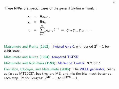
These RNGs are special cases of the general F2-linear family:

xi = Axi−1,

yi = Bxi ,

ui =w∑`=1

yi ,`−12−` = .yi ,0 yi ,1 yi ,2 · · · ,

Matsumoto and Kurita (1992): Twisted GFSR, with period 2k − 1 fork-bit state.

Matsumoto and Kurita (1994): tempered TGFSR.

Matsumoto and Nishimura (1998): Mersenne Twister. MT19937.

Panneton, L’Ecuyer, and Matsumoto (2006): The WELL generator, nearlyas fast as MT19937, but they are ME, and mix the bits much better ateach step. Period lengths: 2512 − 1 to 244497 − 1.

Dra

ft

31

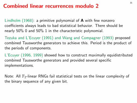
Combined linear recurrences modulo 2

Lindholm (1968): a primitive polynomial of A with few nonzerocoefficients always leads to bad statistical behavior. There should benearly 50% 0 and 50% 1 in the characteristic polynomial.

Tezuka and L’Ecuyer (1991) and Wang and Compagner (1993) proposedcombined Tausworthe generators to achieve this. Period is the product ofthe periods of components.

L’Ecuyer (1996, 1999) showed how to construct maximally equidistributedcombined Tausworthe generators and provided several specificimplementations.

Note: All F2-linear RNGs fail statistical tests on the linear complexity ofthe binary sequence of any given bit.

Dra

ft

32

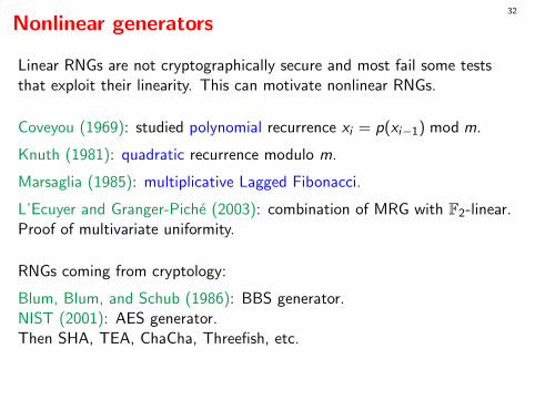
Nonlinear generators

Linear RNGs are not cryptographically secure and most fail some teststhat exploit their linearity. This can motivate nonlinear RNGs.

Coveyou (1969): studied polynomial recurrence xi = p(xi−1) mod m.

Knuth (1981): quadratic recurrence modulo m.

Marsaglia (1985): multiplicative Lagged Fibonacci.

L’Ecuyer and Granger-Piche (2003): combination of MRG with F2-linear.Proof of multivariate uniformity.

RNGs coming from cryptology:

Blum, Blum, and Schub (1986): BBS generator.NIST (2001): AES generator.Then SHA, TEA, ChaCha, Threefish, etc.

Dra

ft

33

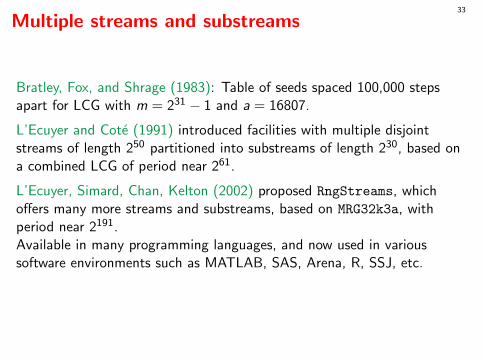
Multiple streams and substreams

Bratley, Fox, and Shrage (1983): Table of seeds spaced 100,000 stepsapart for LCG with m = 231 − 1 and a = 16807.

L’Ecuyer and Cote (1991) introduced facilities with multiple disjointstreams of length 250 partitioned into substreams of length 230, based ona combined LCG of period near 261.

L’Ecuyer, Simard, Chan, Kelton (2002) proposed RngStreams, whichoffers many more streams and substreams, based on MRG32k3a, withperiod near 2191.Available in many programming languages, and now used in varioussoftware environments such as MATLAB, SAS, Arena, R, SSJ, etc.

Dra

ft

33Some key references

Main paper: L’Ecuyer, P. 2017.“History of Uniform Random Number Generation”.In Proceedings of the 2017 Winter Simulation Conference: IEEE Press.

Coveyou, R. R., and R. D. MacPherson. 1967.“Fourier Analysis of Uniform Random Number Generators”.Journal of the ACM 14:100–119.

Knuth, D. E. 1998.The Art of Computer Programming, Volume 2: Seminumerical Algorithms. Thirded.Reading, MA: Addison-Wesley.

L’Ecuyer, P. 2012.“Random Number Generation”.In Handbook of Computational Statistics (second ed.)., edited by J. E. Gentle,W. Haerdle, and Y. Mori, 35–71. Berlin: Springer-Verlag.

L’Ecuyer, P., D. Munger, B. Oreshkin, and R. Simard. 2017.“Random Numbers for Parallel Computers: Requirements and Methods, withEmphasis on GPUs”.Mathematics and Computers in Simulation 135:3–17.Open access at http://dx.doi.org/10.1016/j.matcom.2016.05.005.

L’Ecuyer, P., and F. Panneton. 2009.

Dra

ft

33“F2-Linear Random Number Generators”.In Advancing the Frontiers of Simulation: A Festschrift in Honor of George SamuelFishman, edited by C. Alexopoulos, D. Goldsman, and J. R. Wilson, 169–193. NewYork: Springer-Verlag.

L’Ecuyer, P., and R. Simard. 2007, August.“TestU01: A C Library for Empirical Testing of Random Number Generators”.ACM Transactions on Mathematical Software 33 (4): Article 22.

L’Ecuyer, P., R. Simard, E. J. Chen, and W. D. Kelton. 2002.“An Object-Oriented Random-Number Package with Many Long Streams andSubstreams”.Operations Research 50 (6): 1073–1075.

Lehmer, D. H. 1951.“Mathematical Methods in Large Scale Computing Units”.The Annals of the Computation Laboratory of Harvard University 26:141–146.