Embed Size (px)
Citation preview
Submitted to Operations Researchmanuscript (Please, provide the manuscript number!)
Generalized Likelihood Ratio Method for StochasticModels with Uniform Random Numbers As Inputs
Yijie PengDepartment of Management Science and Information Systems, Guanghua School of Management, Peking University, Beijing,
100871, China, [email protected]
Michael C. FuThe Robert H. Smith School of Business, Institute for Systems Research, University of Maryland, College Park, Maryland
20742-1815, USA, [email protected]
Jiaqiao HuApplied Mathematics & Statistics, College of Engineering and Applied Sciences, Stony Brook University, Stony Brook, NY
11794-3600, USA, [email protected]
Pierre L’EcuyerDepartment of Computer Science and Operations Research, University of Montreal, Montreal, Quebec, Canada,
Bruno TuffinInria, Univ Rennes, CNRS, IRISA, Campus de Beaulieu, 35042 RENNES Cedex, France, [email protected]
We propose a new unbiased stochastic gradient estimator for a family of stochastic models with uniform
random numbers as inputs. By extending the generalized likelihood ratio (GLR) method, the proposed
estimator applies to discontinuous sample performances with structural parameters without requiring that
the tails of the density of the input random variables go down to zero smoothly, an assumption in Peng
et al. (2018) and Peng et al. (2020a) that precludes a direct formulation in terms of uniform random
numbers as inputs. By overcoming this limitation, our new estimator greatly expands the applicability of
the GLR method, which we demonstrate for several general classes of uniform input random numbers,
including independent inverse transform random variates and dependent input random variables governed by
an Archimedean copula. We show how the new derivative estimator works in specific settings such as density
estimation, distribution sensitivity for quantiles, and sensitivity analysis for Markov chain stopping time
problems, which we illustrate with applications to statistical quality control, stochastic activity networks,
and credit risk derivatives. Numerical experiments substantiate broad applicability and flexibility in dealing
with discontinuities in sample performance.
Key words : simulation; stochastic derivative estimation; discontinuous sample performance; uniform
random numbers, generalized likelihood ratio method.
History :
1
Author: GLR with Uniform Random Numbers2 Article submitted to Operations Research; manuscript no. (Please, provide the manuscript number!)
1. Introduction
Stochastic gradient estimation plays a central role in gradient-based optimization and sensitivity
analysis (Asmussen and Glynn, 2007). The finite difference (FD) method is easily implementable,
but it must balance a bias-variance tradeoff and requires extra simulations. Infinitesimal pertur-
bation analysis (IPA) and the likelihood ratio (LR) method are two well-established unbiased
derivative estimation techniques (Glynn, 1990, Ho and Cao, 1991, Glasserman, 1991, Rubinstein
and Shapiro, 1993, Glynn and L’Ecuyer, 1995). IPA typically leads to lower variance than LR
(L’Ecuyer, 1990; Cui et al., 2020), and the weak derivative method reduces the variance of LR
at the cost of performing extra simulations (Pflug, 1988, Heidergott and Leahu, 2010). L’Ecuyer
(1990) provides a general framework unifying IPA and LR, under which the resulting estimator
depends on the choice of what a sample point in a probability space represents, and could in
particular be a hybrid between IPA and LR. See Fu (2015) for a recent review.
Traditional applications of stochastic gradient estimation are in discrete event dynamic systems
(DEDS), including queueing systems (Suri and Zazanis, 1988, Fu and Hu, 1993, L’Ecuyer and
Glynn, 1994), inventory management (Fu, 1994, Bashyam and Fu, 1998), statistical quality con-
trol (Fu and Hu, 1999, Fu et al., 2009b), maintenance systems (Heidergott, 1999, Heidergott and
Farenhorst-Yuan, 2010), and financial engineering and risk management, such as computing finan-
cial derivatives (Fu and Hu, 1995, Broadie and Glasserman, 1996, Liu and Hong, 2011, Wang et al.,
2012, Hong et al., 2014, Chen and Liu, 2014, Lei et al., 2020), value-at-risk (VaR) and conditional
VaR (CVaR) (Hong, 2009, Hong and Liu, 2009, Fu et al., 2009a, Jiang and Fu, 2015, Heidergott
and Volk-Makarewicz, 2016). Recently, stochastic gradient estimation techniques have attracted
attention in machine learning and artificial intelligence; see Mohamed et al. (2020) for a review
paper written by a research team of Google’s DeepMind. Peng et al. (2020b) show pathwise equiva-
lence between IPA and backpropagation, and how the computational complexity for estimating the
Author: GLR with Uniform Random NumbersArticle submitted to Operations Research; manuscript no. (Please, provide the manuscript number!) 3
gradient is reduced by propagating the errors backwardly along the ANN. An LR-based method is
then proposed to train ANNs, which can improve the robustness in classifying images under both
adversarial attacks and natural noise corruptions.
IPA requires continuity in the sample performance, whereas LR does not directly apply for struc-
tural parameters (parameters directly appearing in the sample performance), which significantly
limit their applicability. Smoothed perturbation analysis (SPA) deals with discontinuous sample
performances by using a conditioning technique (Gong and Ho, 1987, Fu and Hu, 1997), but a
good choice of conditioning is problem-dependent. Push-out LR addresses structural parameters
by pushing the parameters out of the sample performance and into the density (Rubinstein and
Shapiro, 1993), which can be achieved alternatively with the IPA-LR in L’Ecuyer (1990), but it
requires an explicit transformation. Recently, Peng et al. (2018) proposed a generalized likelihood
ratio (GLR) method that is capable of dealing with a large scope of discontinuous sample perfor-
mances with structural parameters in a unified framework. The method extends the application
domain of IPA and LR and does not require conditioning and transformation techniques tailored
to specific problem structures.
The GLR method has the virtue of handling many applications in a uniform manner, and it has
been used to deal with discontinuities in financial derivatives, statistical quality control, mainte-
nance systems, and inventory systems (Peng et al., 2016, Peng et al., 2018). Distribution sensitiv-
ities, which mean the derivatives of the distribution function with respect to both the arguments
and the parameters in the underlying stochastic model, lie at the center of many applications such
as quantile sensitivity estimation, confidence interval construction for the quantile and quantile
sensitivities, and statistical inference (Peng et al., 2017, Lei et al., 2018). Peng et al. (2020a) derive
GLR estimators for any order of distribution sensitivities and apply them to maximum likelihood
estimation for complex stochastic models without requiring analytical likelihoods. Glynn et al.
(2020) apply the GLR method to estimate sensitivity of a distortion risk measure, which is a
Lebesgue-Stieltjes integral of quantile sensitivities and includes Var and CVaR as special cases.
Author: GLR with Uniform Random Numbers4 Article submitted to Operations Research; manuscript no. (Please, provide the manuscript number!)
Although the existing GLR method has broad applicability, it requires that the density of the
input distribution is known and that both tails of the density go down to zero smoothly and fast
enough, which may not be satisfied in some applications, depending on what is interpreted as
the input random variables. In this work, we relax this smoothness requirement and establish the
unbiasedness of GLR gradient estimators for stochastic models whose inputs are uniform random
numbers, which are the basic building blocks in generating other random variables. Unlike in Peng
et al. (2018) where the surface integration part for the GLR estimator is zero, the surface integration
part for the GLR estimator in the present work is not necessarily zero but can be estimated by
simulation. If the surface integration part is zero, we are able to relax certain integrability conditions
given in Peng et al. (2018) that are difficult to verify in practice.
We provide specific forms of the GLR estimators for two types of stochastic models and apply the
GLR method to various problem settings, including distribution sensitivities, credit risk financial
derivatives, and statistical quality control. The GLR estimator with independent input random
variables generated from the inverse transform of uniform random numbers reduces to the classic LR
estimator, which indicates that GLR is a generalization of LR from a different perspective than that
of Peng et al. (2018). We also show how GLR can provide sensitivity estimators for models defined
in terms of random vectors with given marginal distributions and whose dependence structures are
specified by Archimedean copulas (Nelsen, 2006). The Gaussian copula has been widely used due
to its simplicity (Li, 2000), and sensitivity analysis for portfolio credit risk derivatives with joint
defaults governed by a Gaussian copula has been studied in Chen and Glasserman (2008) using
LR and SPA. However, the Gaussian copula was widely criticized after the 2008 financial crisis,
because it underestimates the probability of joint defaults. Archimedean copulas (Nelsen, 2006),
not covered in Chen and Glasserman (2008), are relatively easy to simulate and can better capture
the asymmetric tail dependence structure of the joint default data (Embrechts et al., 2003).
GLR can be used to estimate the distribution sensitivity functions, including the density and
the quantile function together with confidence intervals, using a single batch of uniform random
Author: GLR with Uniform Random NumbersArticle submitted to Operations Research; manuscript no. (Please, provide the manuscript number!) 5
numbers. We provide numerical illustrations with various examples. Sample performances of control
charts used in statistical quality control generally involve a stopping time defined by hitting a
control limit (Fu and Hu, 1999, Fu et al., 2009b). The IPA and LR methods do not apply to this
problem due to the discontinuity with respect to the control limits. We formulate a stopping time
problem with uniform random numbers as inputs in a Markov chain, and estimate its sensitivity by
the GLR method. We also apply GLR to estimate distribution sensitivities for stochastic activity
networks (SAN) with uniform random numbers as inputs. In practice, the duration of an activity
in a SAN and the output sample in control charts may be supported on a compact space, so a
distribution supported on the whole space, which was assumed in Peng et al. (2018) and Peng
et al. (2020a), is unsuitable for modeling input distributions in these stochastic models.
The rest of the paper is organized as follows. Section 2 sets the framework. The GLR estimator is
presented in Section 3 with the specific forms of the estimators for two types of models. Applications
are given in Section 4. Numerical experiments can be found in Section 5. The last section concludes.
The technical proofs and additional numerical results can be found in the online appendix.
2. Problem Formulation
Consider a stochastic model of the following form:
ϕ(g(U ;θ)), (1)
where ϕ : Rn → R is a measurable function (not necessarily continuous), g(·;θ) = (g1(·;θ), . . . ,
gn(·;θ)) is a vector of functions gi : (0,1)n→R with certain smoothness properties to be made more
precise shortly, and U = (U1, . . . ,Un) is a vector of i.i.d. U(0,1) random variables (i.e., uniform over
(0,1)). For simplicity, we take θ as a scalar. When θ is a vector, each component of the gradient
can be estimated separately using the method developed in this work. We consider the problem of
estimating the following derivative:
∂E[ϕ(g(U ;θ))]
∂θ. (2)
Author: GLR with Uniform Random Numbers6 Article submitted to Operations Research; manuscript no. (Please, provide the manuscript number!)
A straightforward pathwise derivative estimator, i.e., IPA, obtained by directly interchanging
derivative and expectation, may not apply because discontinuities in the sample performance of the
stochastic model could be introduced by ϕ(·). In Peng et al. (2018), the stochastic model considered
for the derivative estimation problem is ϕ(g(X;θ)), where the density of X = (X1, . . . ,Xn) is
assumed to be known and both tails go down to zero smoothly and fast enough. This assumption
is not satisfied by discontinuous densities, such as the uniform and exponential distributions, and
we want to address this limitation. Before deriving a GLR derivative estimator, we first introduce
two examples to illustrate potential applications of the stochastic model (1).
Example 1 Independent Inputs Generated via the Inverse Transform Method. Suppose
X = (X1, . . . ,Xn) is a vector of independent random variables, where each Xi has cumulative
distribution function (cdf) Fi(·;θ), i= 1, . . . , n, and is generated by (standard) inversion:
Xi = F−1i (Ui;θ), i= 1, . . . , n,
with i.i.d. Ui ∼ U(0,1). A stochastic model with i.i.d. U(0,1) random numbers as input can be
written as ϕ(g(U ;θ)) =ϕ(F−11 (U1;θ), . . . ,F−1
n (Un;θ)), where g(u;θ) = (F−11 (u1;θ), . . . ,F−1
n (un;θ)).
Example 2 Archimedean Copulas. Copulas are a general way of representing the dependence
in a multivariate distribution. A copula is any multivariate cdf whose one-dimensional marginals
are all U(0,1). It can be defined by a function C(·;θ) : [0,1]n→ [0,1] that satisfies certain conditions
required for C to be a consistent cdf; see Nelsen (2006). For any given copula and arbitrary
marginal distributions with continuous cdf’s F1(·),F2(·), ...,Fn(·) with densities fi(·), i= 1, . . . , n,
one can define a multivariate distribution having exactly these marginals with joint cdf FX given
by FX(x) = C(F1(x1),F2(x2), ...,Fn(xn);θ) for all x := (x1, . . . , xn). Sklar (1959) shows that any
multivariate distribution can be represented in this way. If C(·;θ) is absolutely continuous, the
density of the joint distribution is
fX(x;θ) = c (F1(x1), . . . ,Fn(xn);θ)n∏i=1
fi(xi), where
Author: GLR with Uniform Random NumbersArticle submitted to Operations Research; manuscript no. (Please, provide the manuscript number!) 7
c(v;θ) =∂nC(v;θ)
∂v1 · · ·∂vn,
v = (v1, . . . , vn), and the derivative is interpreted as a Radon-Nikodym derivative when C(·;θ) is
not nth-order differentiable.
To generate X = (X1, . . . ,Xn) from the joint cdf FX(·), generate V = (V1, . . . , Vn) from the copula
and return Xi = F−1i (Vi) for each i. Generating V from the copula is not always obvious, but
there are classes of copulas for which this can be easily done, one of them being the Archimedean
copulas. This important family of copulas can model strong forms of tail dependence using a single
parameter, which makes them convenient to use. An Archimedean copula Ca is defined by
Ca(v;θ) =ψθ
(ψ
[−1]θ (v1) + . . .+ψ
[−1]θ (vn)
),
where the generator function ψθ : [0,∞)→ [0,1] is a strictly decreasing convex function such that
limx→∞ψθ(x) = 0, θ ∈ [0,∞) is a parameter governing the strength of dependence, and ψ[−1]θ is a
pseudo-inverse defined by ψ[−1]θ (x) = 10 ≤ x ≤ ψθ(0)ψθ(x), with the convention that ψ−1
θ (0) =
infx : ψθ(x) = 0. Archimedean copulas are absolutely continuous, and their densities have the
form:
ca(v;θ) = 1
0≤
n∑i=1
ψ−1θ (vi)≤ψ−1
θ (0)
∂nψθ(x)
∂xn
∣∣∣∣x=
∑ni=1 ψ
−1θ
(vi)
n∏i=1
∂ψ−1θ (vi)
∂vi,
assuming that the generator function ψθ(·) is smooth (Nelsen, 2006). In general we do not have
an analytical expression for ca(·;θ), and it can be discontinuous in θ. Therefore, the standard LR
method typically does not apply to sensitivity analysis with Archimedean copulas.
Marshall and Olkin (1988) propose the following simple algorithm to generate V from an
Archimedean copula with generator function ψθ(·):
(i) Generate a random variable Yθ from the distribution with Laplace transform ψθ(·) (with at
least one uniform random number as input).
(ii) For i= 1, . . . , n, let Vi =ψθ (−(logUi)/Yθ) with i.i.d. Ui ∼U(0,1).
For a given Yθ, this gives a stochastic model with uniform random numbers Ui as inputs:
ϕ(g(U ;θ)) = φ(F−1
1 (ψθ (−(logU1)/Yθ)) , . . . ,F−1n (ψθ (−(logUn)/Yθ))
),
where ϕ(v1, . . . , vn) = φ(F−11 (v1), . . . ,F−1
1 (vn)) and g(u;θ) = (ψθ (−(logu1)/Yθ) , . . . ,ψθ (−(logun)/Yθ)).
Author: GLR with Uniform Random Numbers8 Article submitted to Operations Research; manuscript no. (Please, provide the manuscript number!)
3. A Generalized Likelihood Ratio Method
In this section, we derive the GLR estimator for the derivative (2) of the expectation of stochastic
model (1). The general theory for GLR is first derived, and then it is applied to the two examples
in the previous section.
3.1. General Theory
Denote the Jacobian of g by
Jg(u;θ) :=
∂g1(u;θ)
∂u1
∂g1(u;θ)
∂u2· · · ∂g1(u;θ)
∂un
∂g2(u;θ)
∂u1
∂g2(u;θ)
∂u2· · · ∂g2(u;θ)
∂un
......
. . ....
∂gn(u;θ)
∂u1
∂gn(u;θ)
∂u2· · · ∂gn(u;θ)
∂un
, and
∂θg(u;θ) :=
(∂g1(u;θ)
∂θ, . . . ,
∂gn(u;θ)
∂θ
)T,
with the superscript T indicating vector transposition. In addition, we define two weight functions
in the GLR estimator:
ri(u;θ) :=
(J−1g (u;θ) ∂θg(u;θ)
)Tei, i= 1, . . . , n, (3)
d(u;θ) :=n∑i=1
eTi J−1g (u;θ) (∂uiJg(u;θ))J−1
g (u;θ)∂θg(u;θ)− trace(J−1g (u;θ) ∂θJg(u;θ)), (4)
where ei is the ith unit column vector and ∂zJg is the matrix obtained by differentiating Jg with
respect to z element-wise. Let x− and x+ be limits taken from the left-hand side and right-hand side
of x, respectively, and for a function h(·), denote h(x−) := limx→x− h(x) and h(x+) := limx→x+ h(x).
The following conditions are introduced to guarantee the unbiasedness of the proposed GLR deriva-
tive estimator.
(A.1) There exist a smooth function ϕε(·)∈C∞ and p > 1 such that
limε→0
supθ∈Θ
∫(0,1)n
|ϕε(g(u;θ))−ϕ(g(u;θ))|p du= 0,
Author: GLR with Uniform Random NumbersArticle submitted to Operations Research; manuscript no. (Please, provide the manuscript number!) 9
and if n> 1, for a fixed ε > 0 and any ui ∈ (0,1) \ [ε,1− ε], i= 1, . . . , n,
limε→0
supθ∈Θ
∫(0,1)n−1
|ϕε(g(u;θ))−ϕ(g(u;θ))|p du−i = 0,
where u−i := (u1, . . . , ui−1, ui+1, . . . , un), and if n= 1, for any u∈ (0,1) \ [ε,1− ε],
limε→0
supθ∈Θ
|ϕε(g(u;θ))−ϕ(g(u;θ))|= 0.
(A.2) The Jacobian Jg(u;θ) is invertible almost everywhere (a.e.), and the performance function
g(u;θ) is twice continuously differentiable with respect to (u, θ)∈ (0,1)n×Θ, where Θ is a bounded
neighborhood of the parameter θ of interest.
(A.3) The following integrability conditions hold:
∫(0,1)n−1
supθ∈Θ,ui∈(0,1)
∣∣ϕ(g(u;θ)) ri(u;θ)∣∣ du−i <∞, i= 1, . . . , n, and
∫(0,1)n
supθ∈Θ
∣∣ϕ(g(u;θ)) d(u;θ)∣∣ du<∞.
(A.4) The function g(·;θ) is invertible, and
limui→1−
supθ∈Θ,u−i∈(0,1)n−1
|ri(u;θ)|= limui→0+
supθ∈Θ,u−i∈(0,1)n−1
|ri(u;θ)|= 0, i= 1, . . . , n.
Remark 1 Condition (A.1) can be checked in certain settings when ϕε(·) can be explicitly con-
structed; see Proposition 1. The invertibility of the Jacobian matrix in condition (A.2) justifies
the local invertibility of function g(·;θ), whereas global invertibility of g(·;θ) in condition (A.4) is
stronger, although much weaker than requiring an explicit inverse function for g(·;θ) in deriving
the push-out LR estimator (Rubinstein and Shapiro, 1993). In general, it is difficult to find an
explicit inverse function for a nonlinear function g(·;θ), but the existence of the inversion could be
guaranteed by the inverse function theorem.
Unbiasedness of the new GLR estimator developed in this work is established under two sets of
conditions in the following theorem.
Author: GLR with Uniform Random Numbers10 Article submitted to Operations Research; manuscript no. (Please, provide the manuscript number!)
Theorem 1 Under conditions (A.1) – (A.3) or (A.2) – (A.4),
∂E[ϕ(g(U ;θ))]
∂θ=E[G(U ;θ)], where (5)
G(U ;θ) :=n∑i=1
[ϕ(g(U i;θ))ri(U i;θ)−ϕ(g(U i;θ))ri(U i;θ)
]+ϕ(g(U ;θ))d(U ;θ),
with U i := (U1, . . . , 1−︸︷︷︸ith element
, . . . ,Un), U i := (U1, . . . , 0+︸︷︷︸ith element
, . . . ,Un), and ri(·) and d(·) defined by
(3) and (4), respectively.
Remark 2 The proof of the theorem can be found in the online Appendix A. Even if g(U i;θ) =∞
or g(U i;θ) =∞, the GLR estimator could still be well defined; see e.g. Section 3.1. The difference
between this estimator and the GLR estimator in Peng et al. (2018) is that the surface integration
part in Peng et al. (2018) is shown to be zero under certain conditions including that the tails of
the input densities are required to go to zero smoothly and fast enough, whereas here the surface
integration part is included in the estimator and can be estimated by simulation. In the case where
the surface integration part becomes zero, we can prove the result without assuming (A.1), and we
also avoid the integrability condition in Peng et al. (2018) on certain intermediate quantities (the
smoothed function), which is difficult to verify in practice. The proof is obtained by first truncating
the support of the input random variables to a compact set and then appropriately expanding it
to the whole space.
We now examine the special case where g(u;θ) = (g1(u1;θ), . . . , gn(un;θ)), which covers Exam-
ples 1 and 2. For n independent uniform random numbers, we can take gi(ui;θ) = F−1i (ui;θ) for
i = 1, . . . , n, while for dependent variables governed by an Archimedean copula, conditional on
Yθ = y, we have gi(ui;θ) =ψθ(− logui/y) for i= 1, . . . , n. In this special case, the Jacobian becomes
Jg(u;θ) =
∂g1(u1;θ)
∂u10 · · · 0
0 ∂g2(u2;θ)
∂u2· · · 0
......
. . ....
0 0 · · · ∂gn(un;θ)
∂un
.
Author: GLR with Uniform Random NumbersArticle submitted to Operations Research; manuscript no. (Please, provide the manuscript number!) 11
Then we have
ri(u;θ) =∂gi(ui;θ)
∂θ
/∂gi(ui;θ)
∂ui, i= 1, . . . , n, and
d(u;θ) =n∑i=1
[∂gi(ui;θ)
∂θ
∂2gi(ui;θ)
∂u2i
/(∂gi(ui;θ)
∂ui
)2
− ∂2gi(ui;θ)
∂θ∂ui
/∂gi(ui;θ)
∂ui
].
Moreover, condition (A.1) in Theorem 1 can be replaced by a set of a simpler assumptions when
the performance function ϕ(x) is a product of n indicators: ϕ(x) =∏n
i=1 1xi ≤ 0, in which case a
smoothed function ϕε(·) can be constructed explicitly. The performance function in the distribution
sensitivities discussed in Section 4.1 is an indicator function. The distribution sensitivities for the
completion time in an SAN in Section 5.2 and the sensitivities of a control chart in Section 5.3 have
performance functions which are products of n indicators. The proof of the following proposition
can be found in the online Appendix A.
Proposition 1 Consider the stochastic model
ϕ(g(U ;θ)) =n∏i=1
1gi(Ui;θ)≤ 0.
Condition (A.1) holds if for i= 1, . . . , n and a fixed ε > 0 in (6),
infθ∈Θ,ui∈[ε,1−ε]
∣∣∣∣∂gi(ui;θ)∂ui
∣∣∣∣> 0 and infθ∈Θ,ui∈(0,1)\[ε,1−ε]
∣∣gi(ui;θ)∣∣> 0. (6)
If the functions gi can be decomposed as products of the form gi(ui;θ) = ξi(θ)ηi(ui) for i =
1, . . . , n, then conditions (A.3), (A.4), and (6) can be simplified. For example, an exponential
random variable with mean θ can be generated by − log(Ui)/θ where Ui ∼ U(0,1). When this
decomposition holds, we can write
ri(u;θ) =d log ξi(θ)
dθ
/d log ηi(ui)
dui, i= 1, . . . , n, and
d(u;θ) =n∑i=1
d log ξi(θ)
dθ
[ηi(ui)η
′′i (ui)
(η′i(ui))2 − 1
].
Author: GLR with Uniform Random Numbers12 Article submitted to Operations Research; manuscript no. (Please, provide the manuscript number!)
(A.3’) Boundedness and integrability conditions on functions of input random numbers:
infui∈(0,1)
∣∣∣∣d log ηi(ui)
dui
∣∣∣∣> 0 and E
[∣∣ηi(Ui)η′′i (Ui)∣∣
(η′i(Ui))2
]<∞, i= 1, . . . , n.
(A.4’) Boundary condition on functions of input random numbers:
limui→1−
∣∣∣∣d log ηi(ui)
dui
∣∣∣∣= limui→0+
∣∣∣∣d log ηi(ui)
dui
∣∣∣∣=∞, i= 1, . . . , n.
Corollary 1 Suppose that gi(ui;θ) = ξi(θ)ηi(ui), i= 1, . . . , n, and ϕ(·) is bounded and
maxi=1,...,n
supθ∈Θ
∣∣∣∣∂ log ξi(θ)
∂θ
∣∣∣∣<∞.Then conditions (A.3) and (A.4) can be replaced by (A.3’) and (A.4’), respectively, and condition
(6) in Proposition 1 also simplifies to
infθ∈Θ
∣∣ξi(θ)|> 0, infui∈[ε,1−ε]
∣∣∣∣η′i(ui)∣∣∣∣> 0, infui∈(0,1)\[ε,1−ε]
∣∣ηi(ui)∣∣> 0, i= 1, . . . , n.
Unbiasedness of the GLR estimators in many examples of this paper can be justified by verifying
these simplified conditions.
3.2. The Independent Case
Let us return to the independent case of Example 1 and suppose that each Xi is continuous with
density fi(·;θ). Our goal is to estimate
∂E[ϕ(F−11 (U1;θ), . . . ,F−1
n (Un;θ))]
∂θ, for which the Jacobian is
Jg(u;θ) =
1f1(X1(u1;θ);θ)
0 · · · 0
0 1f2(X2(u2;θ);θ)
· · · 0
......
. . ....
0 0 · · · 1fn(Xn(un;θ);θ)
, and
∂θg(u;θ) =
(∂X1(u1;θ)
∂θ, . . . ,
∂Xn(un;θ)
∂θ
)T,
Author: GLR with Uniform Random NumbersArticle submitted to Operations Research; manuscript no. (Please, provide the manuscript number!) 13
where Xi(ui;θ) := F−1i (ui;θ) and
∂Xi(ui;θ)
∂θ:=−∂Fi(xi;θ)
∂θ
/fi(xi;θ)
∣∣∣∣xi=Xi(ui;θ)
.
Then the weight functions in the GLR estimator are:
ri(u;θ) =−∂Fi(xi;θ)∂θ
∣∣∣∣xi=Xi(ui;θ)
and d(u;θ) =n∑i=1
∂ log fi(xi;θ)
∂θ
∣∣∣∣xi=Xi(ui;θ)
, so
limui→1−
ri(u;θ) = limui→0+
ri(u;θ) = 0.
Therefore,∂E[ϕ(F−1
1 (U1;θ), . . . ,F−1n (Un;θ))]
∂θ=E
[ϕ(F−1
1 (U1;θ), . . . ,F−1n (Un;θ)) d(U ;θ)
]=E
[ϕ(X)
n∑i=1
∂ log fi(Xi;θ)
∂θ
].
The expression inside the last expectation coincides with the classic LR derivative estimator in
the case where the LR method is applicable, i.e., when there are no structural parameters in the
sample performance (Glynn, 1990). From this perspective, the GLR method generalizes the LR
method by allowing the appearance of structural parameters.
3.3. Archimedean Copulas
We consider estimating
∂
∂θE[ϕ
(ψθ(− logU1
Yθ
), . . . ,ψθ
(− logUn
Yθ
))],
where the expectation is with respect to both Yθ and the independent Ui, i= 1, . . . , n. By condi-
tioning, we can use a mixture of LR and GLR:
∂
∂θE[ϕ
(ψθ(− logU1
Yθ
), . . . ,ψθ
(− logUn
Yθ
))]= E
[ϕ
(ψθ(− logU1
Yθ
), . . . ,ψθ
(− logUn
Yθ
))∂ log fY (y;θ)
∂θ
∣∣∣∣y=Yθ
]
+E
∂E[ϕ
(ψθ(− logU1
y
), . . . ,ψθ
(− logUn
y
))]∂θ
∣∣∣∣∣∣∣∣y=Yθ
,(7)
where fY (·;θ) is the density function of Yθ. This equality follows from Theorem 1 of
L’Ecuyer (1990) with ω in that theorem replaced by y and h(θ,ω) replaced by h(y, θ) :=
Author: GLR with Uniform Random Numbers14 Article submitted to Operations Research; manuscript no. (Please, provide the manuscript number!)
E[ϕ(ψθ(− lnU1/y), . . . ,ψθ(− lnUn/y))], under the assumption that for all y, this last expectation
is continuous in θ and differentiable except perhaps on a countable set. Specifically, (7) can be
rewritten as
∂
∂θ
∫Rh(y, θ)FY (dy;θ) =
∂
∂θ
∫Rh(y, θ)L(y, θ, θ0)FY (dy;θ0)
=
∫R
(h(y, θ)
∂L(y, θ, θ0)
∂θ+∂h(y, θ)
∂θL(y, θ, θ0)
)FY (dy;θ0),
where L(y, θ, θ0) := fY (y;θ)/fY (y;θ0). The first term on the right-hand side of (7) can be dealt
with by the LR method straightforwardly if fY (·;θ) admits an analytical form. Glasserman and
Liu (2010) show how to apply the LR method with only the Laplace transform ψθ(·).
We now show how to use GLR to handle the second term on the right-hand side of (7) with Yθ
fixed and generated from other uniform random numbers. The Archimedean copula model falls into
the special case where g(u;θ) = (g1(u1;θ), . . . , gn(un;θ)), discussed after Theorem 1. The Jacobian
in this case is
Jg(u;θ, y) =
− 1u1y
ψ′θ(− logu1
y
)0 · · · 0
0 − 1u2y
ψ′θ(− logu2
Yθ
)· · · 0
......
. . ....
0 0 · · · − 1uny
ψ′θ(− logun
y
)
, and
∂θg(u;θ, y) =
(∂ψθ(x1)
∂θ
∣∣∣∣x1=− logu1
y
, . . . ,∂ψθ(xn)
∂θ
∣∣∣∣xn=− logun
y
)T.
The weight functions in the GLR estimator are
ri(u;θ, y) =− uiy
ψ′θ(xi)
∂ψθ(xi)
∂θ
∣∣∣∣xi=−
loguiy
,
d(u;θ, y) =n∑i=1
(− 1
ψ′θ(xi)
∂ψ′θ(xi)
∂θ+
ψ′′θ (xi)
(ψ′θ(xi))2
∂ψθ(xi)
∂θ+∂ψθ(xi)
∂θ
y
ψ′θ(xi)
)∣∣∣∣xi=−
loguiy
.
Example 3 The Clayton Copula. The generator function for the Clayton copula is
ψθ(x) = (1 +x)−1θ , θ ∈ (0,∞).
Author: GLR with Uniform Random NumbersArticle submitted to Operations Research; manuscript no. (Please, provide the manuscript number!) 15
Then,∂ψθ(x)
∂θ=
1
θ2log(1 +x)(1 +x)−
1θ ,
∂ψ′θ(x)
∂θ=
1
θ2(1 +x)−
1θ−1
[1− 1
θlog(1 +x)
], and
ψ′θ(x) =−1
θ(1 +x)−
1θ−1, ψ
′′θ (x) =
1
θ
(1
θ+ 1
)(1 +x)−
1θ−2.
By the inverse Laplace transformation, we find that Yθ ∼ Γ(1/θ,1), the gamma distribution with
density fY (y;θ) = y1θ−1e−y
Γ(1/θ), where Γ(s) :=
∫∞0ts−1e−tdt, and the LR term is
∂ log fY (y;θ)
∂θ=−d log Γ(1/θ)
dθ− 1
θ2log y.
The weight functions in the GLR estimator are
ri(u;θ, y) =−1
θuiy
(1− logui
y
)log
(1− logui
y
),
d(u;θ, y) =n∑i=1
1
θ[1 + (1− (xi + 1)y) log(1 +xi)]
∣∣∣∣xi=−
loguiy
.
In addition, we have limui→0+ ri(u;θ, y) = limui→1− ri(u;θ, y) = 0.
GLR for Ali-Mikhail-Haq copulas can be found in the online Appendix A. For both the Clayton
and Ali-Mikhail-Haq copulas, conditions (A.2) and (A.4) in Theorem 1 are satisfied. If ϕ(·) is
bounded, condition (A.3) in Theorem 1 can also be verified straightforwardly for any y= Yθ.
4. Applications
We apply the GLR method to distribution sensitivity estimation, and estimate sensitivities for
stopping time problems and credit risk derivatives, with specific forms for the function ϕ(·).
4.1. Distribution Sensitivities
For g(·;θ) : (0,1)n→R, we estimate the following two first-order distribution sensitivities:
∂F (z;θ)
∂θ=∂E[1g(U ;θ)− z ≤ 0]
∂θ=E
[∂E[1g(Ui,U−i;θ)− z ≤ 0|U−i]
∂θ
],
f(z;θ) =∂E[1g(U ;θ)− z ≤ 0]
∂z=E
[∂E[1g(Ui,U−i;θ)− z ≤ 0|U−i]
∂z
],
where f(·;θ) is the density function of Z(θ) = g(U ;θ) and U−i := (U1, . . . ,Ui−1,Ui+1, . . . ,Un), i =
1, . . . , n. By applying GLR, we obtain
E[∂E[1g(Ui,U−i;θ)− z ≤ 0|U−i]
∂θ
]=E[G1,i(U ;z, θ)], where
G1,i(U ;z, θ) := 1g(U i;θ)− z ≤ 0ri(U i;θ)−1g(U i;θ)− z ≤ 0ri(U i;θ) +1g(U ;θ)− z ≤ 0d(U ;θ),
Author: GLR with Uniform Random Numbers16 Article submitted to Operations Research; manuscript no. (Please, provide the manuscript number!)
ri(u;θ) =
(∂g(u;θ)
∂ui
)−1∂g(u;θ)
∂θ, and
d(u;θ) =
(∂g(u;θ)
∂ui
)−1[(
∂g(u;θ)
∂ui
)−1∂g(u;θ)
∂θ
∂2g(u;θ)
∂u2i
− ∂2g(u;θ)
∂ui∂θ
].
We also obtain E[∂E[1g(Ui,U−i;θ)− z ≤ 0|U−i]
∂z
]=E[G2,i(U ;z, θ)], where
G2,i(U ;z, θ) :=1g(U i;θ)− z ≤ 0ri(U i;θ)−1g(U i;θ)− z ≤ 0ri(U i;θ)
+1g(U ;θ)− z ≤ 0d(U ;θ), with
ri(u;θ) =−(∂g(u;θ)
∂ui
)−1
and d(u;θ) =−(∂g(u;θ)
∂ui
)−2∂2g(u;θ)
∂u2i
.
To establish the unbiasedness of G1,i(U ;z, θ) and G2,i(U ;z, θ) conditional on U−i, condition (A.1)
in Theorem 1 can be justified by checking the conditions in Proposition 1. Given this conditional
unbiasedness, the unconditional unbiasedness of G1,i(U ;z, θ) and G2,i(U ;z, θ) will follow from
E[supθ∈Θ
|E[G1,i(U ;z, θ)|U−i]]<∞ and E
[supz∈Z|E[G2,i(U ;z, θ)|U−i]|
]<∞,
where Z is a neighborhood of z. Since the indicator function is bounded, the conditions of Propo-
sition 1 follow from the integrability condition on the weight functions: for i= 1, . . . , n,
E[supθ∈Θ
|ri(U i;θ)]
]<∞, E
[supθ∈Θ
|ri(U i;θ)]
]<∞, E
[supθ∈Θ
|d(U ;θ)]
]<∞, and
E[|ri(U i;θ)]
]<∞, E [|ri(U i;θ)]]<∞, E
[|d(U ;θ)]
]<∞.
The GLR estimator for estimating the distribution sensitivities is not unique. We can consider the
above GLR estimator for each i and construct the following linear combination of these n GLR
estimators with real-values weights wi, as in Hammersley and Handscomb (1964, p.19):
n∑i=1
wiGr,i(U ;z, θ) subject ton∑i=1
wi = 1, r= 1,2.
An optimal GLR estimator, which minimizes the variance, can be obtained by solving
arg min(w1,...,wn)
Var
(n∑i=1
wiGr,i(U ;z, θ)
)subject to
n∑i=1
wi = 1.

Author: GLR with Uniform Random NumbersArticle submitted to Operations Research; manuscript no. (Please, provide the manuscript number!) 17
This leads to the optimal weights
w∗i =eTi Σ−1e
eTΣ−1e, i= 1, . . . , n, (GLR-Opt)
where e = (1, . . . ,1)T , ei is a d-dimensional unit vector in ith direction, and Σ = (Σi′i)n×n is the
covariance matrix of (Gr,1(U ;z, θ), . . . ,Gr,n(U ;z, θ)). In practice, w∗i ’s must be estimated, and such
estimators wiil be correlated with the Gr,i. This linear combination idea is equivalent to a control
variate formulation.
Example 4 Distribution Sensitivities for Quantiles. For 0≤ α≤ 1, the α-VaR (or α-quantile)
of a random variable Z(θ) = g(U ;θ) with cdf F (·;θ) is defined as
qα(θ) := arg minz : F (z;θ)≥ α.
When F (·;θ) is continuous, qα(θ) = F−1(α;θ). Let U (j), j = 1, . . . ,m, be i.i.d. realizations of U ∼
U(0,1)d, and Fm(·) be the empirical distribution of Zj := g(U (j);θ), j = 1, . . . ,m. The empirical
α-quantile F−1m (α), which is the inverse of the empirical distribution evaluated at α, is simply
Z(dαme), where Z(1) < · · ·< Z(m) are the realizations of Z1, . . . ,Zm sorted in increasing order (the
order statistics), and dxe denotes the smallest integer greater than or equal to x. This empirical
quantile satisfies the following central limit theorem (Serfling, 1980):
√m(F−1m (α)− qα(θ)
)d→N
(0,
α(1−α)
f(qα(θ);θ)
).
Traditionally, batching and sectioning techniques are used to estimate the asymptotic variance to
construct a confidence interval on the empirical quantile, and these methods lead to subcanonical
convergence rates (Nakayama, 2014). With the GLR density estimator, however, we can estimate
the asymptotic variance by
mα(1−α)∑m
j=1G2,i(U (j);z, θ)|z=F−1m (α)
,
using the same realizations of the uniform random variables U (j) as in the quantile estimator
F−1m (α). It follows from Peng et al. (2017) that this asymptotic variance estimator is consistent.
Author: GLR with Uniform Random Numbers18 Article submitted to Operations Research; manuscript no. (Please, provide the manuscript number!)
We can also estimate the quantile sensitivity q′α(θ) = ∂qα(θ)/∂θ by estimating distribution sen-
sitivities. By the implicit function theorem,
q′α(θ) =−∂F (z;θ)
∂θ
∣∣∣∣z=qα(θ)
/f(qα(θ);θ),
so the quantile sensitivity can be estimated by the ratio
D(θ) :=−∑m
j=1G1,i(U(j);z, θ)∑m
j=1G2,i(U (j);z, θ)
∣∣∣∣z=F−1
m (α)
.
This ratio estimator is biased, because the expectation of the ratio is not equal to the ratio of
expectations and also because of the bias in the quantile estimator, but from Peng et al. (2017), it
is consistent and obeys a central limit theorem when m→∞. Its asymptotic variance can also be
estimated by the GLR estimator for higher-order distribution sensitivities (Peng et al., 2020a).
4.2. Stopping Time Problems
In this subsection, we consider estimating the derivative of the expectation of a sample performance
that depends on a stopping time N :
∂E [ϕN(X1, . . . ,XN)]
∂θ, (8)
where Xi, i≥ 1 is a Markov chain defined by the following stochastic recurrence:
X1 = g1(U1;θ), Xi = κ(Xi−1, gi(Ui;θ)), (9)
and N is the first time the Markov chain hits a set Ω, i.e.,
N =minn∈N : Xn ∈Ω= minn∈N : κ(Xn−1, gn(Un;θ))∈Ω .
The expectation of this sample performance can be rewritten as
E [ϕN(X1, . . . ,XN)] =∞∑n=1
E
[ϕn(X1, . . . ,Xn)
n−1∏i=1
1Xi /∈Ω1Xn ∈Ω
]. (10)
Author: GLR with Uniform Random NumbersArticle submitted to Operations Research; manuscript no. (Please, provide the manuscript number!) 19
For each expectation in the summation on the right-hand side of the equation, the stochastic
model falls into the special case g(u;θ) = (g1(u1;θ), . . . , gn(u1;θ)) discussed after Theorem 1, and
the derivative of can be estimated by the GLR method. We have
∂E [ϕN(X1, . . . ,XN)]
∂θ=∞∑n=1
n∑i=1
E
[ϕn(X+i
1 , . . . ,X+in )
n−1∏j=1
1X+ij /∈Ω1X+i
n ∈Ωri(1−;θ)
]
−∞∑n=1
n∑i=1
E
[ϕn(X−i1 , . . . ,X−in )
n−1∏j=1
1X−ij /∈Ω1X−in ∈Ωri(0+;θ)
]
+∞∑n=1
E
[ϕn(X1, . . . ,Xn)
n−1∏i=1
1Xi /∈Ω1Xn ∈Ωdn(U1, . . . ,Un;θ)
],
where X+ij , j ≥ 1 and X−ij , j ≥ 1 are Markov chains generated by (9) with Ui replaced by 1
and 0, respectively, and dn(·;θ) denotes the second part in the GLR estimator for the nth term
on the right-hand side of (10). We use the randomization technique of Rhee and Glynn (2015) to
obtain a single-run unbiased estimator of (8), which is given by
1
p(N ′)SN ′(U1, . . . ,UN ′) +DN(U1, . . . ,UN), (11)
where N ′ is a discrete random variable supported on Z+ with probability mass function p(·),
Sn(U1, . . . ,Un) :=n∑i=1
ϕn(X+i1 , . . . ,X+i
n )n−1∏j=1
1X+ij /∈Ω1X+i
n ∈Ωri(1−;θ)
−n∑i=1
ϕn(X−i1 , . . . ,X−in )n−1∏j=1
1X−ij /∈Ω1X−in ∈Ωri(0+;θ), and
Dn(U1, . . . ,Un) := ϕn(X1, . . . ,Xn)n−1∏i=1
1Xi /∈Ω1Xn ∈Ωdn(U1, . . . ,Un;θ).
This stopping time problem generalizes those in Glynn (1987) and Heidergott and Vazquez-Abad
(2009) by allowing the distribution of the stopping time N to depend on parameter θ. The classical
IPA and LR methods do not cover this case. In the next example, we discuss sensitivity analysis
for control charts, widely used in statistical quality control.
Example 5 Controls Charts. Control charts aim to detect (statistically) when a manufacturing
or business process goes out of control. The system is assumed to output samples having different
Author: GLR with Uniform Random Numbers20 Article submitted to Operations Research; manuscript no. (Please, provide the manuscript number!)
statistical distributions when in control versus when out of control. The systems goes out of control
at the (unobservable) random time χ with cdf F0(·). The output Zi of the ith sample has cdf
F1(·) when in control and F2(·) when out of control. For an exponentially weighted moving average
(EWMA) chart, the (observable) test statistic after the ith sample is Yi = αZi + (1 − α)Yi−1.
The stopping time N is the time when the system is declared out of control: N = mini : Yi /∈
[θ1, θ2] = mini : Xi /∈ [0,1], where θ1 and θ2 are fixed lower and upper control limits for the
test statistic, and Xi = Yi−θ1θ2−θ1
. Note that Xi, i≥ 1 is a Markov chain that follows the recursion
Xi = (1−α)Xi−1 + gi(Ui;θ), where
gi(Ui;θ) =α
θ2− θ1
[1i < χ/∆F−1
1 (Ui) +1i≥ χ/∆F−12 (Ui)− θ1
],
and ∆ is the sampling period (the time between any two successive monitoring epochs).
Here we consider sensitivity analysis with respect to θ = θ2. This model falls into the spe-
cial case of Corollary 1 where gi(ui;θ) = ξi(θ)ηi(ui), with ξi(θ) = α/(θ − θ1) and ηi(ui) = 1i <
χ/∆F−11 (ui) +1i≥ χ/∆F−1
2 (ui)− θ1, for i= 1, . . . , n. Then we have
ri(u;θ) =− 1
θ2− θ1
[1i < χ/∆F−1
1 (ui)f1(F−11 (ui)) +1i≥ χ/∆F−1
2 (ui)f2(F−12 (ui))− θ1
], and
d(u;θ) =1
θ2− θ1
n∑i=1
[1i < χ/∆ F−1
1 (ui)
f1(F−11 (ui))
+1i≥ χ/∆ F−12 (ui)
f2(F−12 (ui))
+ 1
].
Suppose we pay a cost of c per unit of time when the system is out of control and this is not yet
detected, and a one-time cost C to fix the system when it is declared out of control. This model is
a regenerative process, which regenerates each time we fix the system. The expected cost over one
regenerative cycle is cE[(N − dχ/∆e)+] +C, and therefore the average cost per unit of time over
an infinite horizon iscE[(N −dχ/∆e)+] +C
E[N ]. (12)
The goal might be to select the control limits θ1 and θ2 to minimize this average cost. Widening the
gap θ2−θ1 would reduce the frequency of intervention, so we would pay the fixed cost C less often,
but then the penalty c would be paid over longer periods of time on average. The optimal control
Author: GLR with Uniform Random NumbersArticle submitted to Operations Research; manuscript no. (Please, provide the manuscript number!) 21
limits achieve an optimal balance between these two types of costs. The sample performance of the
expectation in the numerator of (12) is different from those treated by SPA in Fu and Hu (1999)
and Fu et al. (2009b), the development of which depends on the specific structure of the problem.
The GLR method in our work provides unbiased derivative estimators for the expectations in both
the numerator and denominator of (12).
4.3. Credit Risk Derivatives
We consider two important types of credit risk derivatives: basket default swaps (BDSs) and
collateralized debt obligations (CDOs). In a BDS contract, the buyer pays fixed premia p1, ..., pk
to the protection seller at dates 0<T1 < . . . < Tk <T , and if the ith default time τ(i) occurs before
T , i.e., τ(i) <T , these premium payments stop, and the seller undertakes the loss of the ith default
and makes a payment to the buyer. Let Li be the loss of the ith default. The discounted value
of the ith default swap is the difference between the discounted payments made by the seller and
those made by the buyer:
Vbds(τ) = Vvalue(τ)−Vprot(τ),
where Vprot(τ) is the discounted premium payed by the buyer:
Vprot(τ) =
∑`
j=1 pj exp(−rTj) + p`+1 exp(−rτ(i))τ(i)−T`T`+1−T`
, if T` ≤ τ(i) ≤ T`+1,∑k
j=1 pi exp(−rTj), if τ(i) >T,
and Vvalue(X) the discounted payment made by the seller:
Vvalue(X) =L(i) exp(−rτ(i))1τ(i) <T.
In a CDO, the losses caused by the defaults of the assets in the portfolio are packaged together
and then tranched. The tranches are ordered so that losses are absorbed sequentially following the
order of the tranches. For example, a tranche of a CDO absorbs the loss above a threshold L− and
below a threshold L+, i.e.,
Vcdo(τ) = (L−L−) ·1L>L−− (L−L+) ·1L>L+, where
L=n∑i=1
Li ·1τi <T.

Author: GLR with Uniform Random Numbers22 Article submitted to Operations Research; manuscript no. (Please, provide the manuscript number!)
Suppose that the vector of default times (τ1, . . . , τn) have a joint distribution with marginal cdf’s
Fi(·), i= 1, . . . , n, and a dependence structure modeled by an Archimedean copula. Then we can
generate τi’s by generating V = (V1, . . . , Vn) from the copula, and putting τi = F−1i (Vi), i= 1, . . . , n.
The sample performances Vvalue(τ), Vprot(τ), and Vcdo(τ) may be discontinuous with respect to
the structural parameter θ in the copula model due to the presence of indicator functions and
order indices. As a result, neither IPA nor LR can be applied directly for this model. On the other
hand, Vvalue(τ), Vprot(τ), and Vcdo(τ) are all of the form ϕ(g(U ;θ)) that fits our framework, due to
the generality of the measurable function ϕ(·). Unlike in Lei et al. (2020) where a separate CMC
technique needs to be derived for each type of cash flow, the GLR method in this work can estimate
the derivative of the expectation for all three types of cash flows.
5. Numerical Experiments
In this section, we present numerical examples to demonstrate broad applicability and flexibility of
the proposed GLR method to estimate sensitivities in various situations. The examples include an
indicator function applied to a linear combination of two exponential random variables, a stochastic
activity network (SAN), control charts, and a CDO model.
5.1. Distribution Sensitivities for a Linear Model
We estimate distribution sensitivities where ϕ(·) is an indicator function for a linear combination
of two independent exponential random variables with means 1/λ1 and 1/λ2, i.e.,
ϕ(g(U ;θ)) = 1g(U ;θ)≤ z where g(U ;θ) =− θ
λ1
log(U1)− 1
λ2
log(U2).
This sample performance falls into the special case stated in Corollary 1, and the conditions in
Proposition 1 and the integrability condition on the weight function discussed in Section 4.1 can
be checked straightforwardly. We have
∂g(u;θ)
∂u1
=− θ
λ1u1
,∂g(u;θ)
∂u2
=− 1
λ2u2
,∂g(u;θ)
∂θ=− 1
λ1
logu1, and
∂2g(u;θ)
∂u21
=θ
λ1u21
,∂2g(u;θ)
∂u22
=1
λ2u22
,∂2g(u;θ)
∂θ∂u1
=− 1
λ1u1
,∂2g(u;θ)
∂θ∂u2
= 0.
Author: GLR with Uniform Random NumbersArticle submitted to Operations Research; manuscript no. (Please, provide the manuscript number!) 23
0 2 4 6 8 10
z
0
0.05
0.1
0.15
0.2
0.25
0.3
0.35
0.4S
en
sitiv
ity v
alu
e
(a) Distribution sensitivity curve.
0 2 4 6 8 10
z
0
0.05
0.1
0.15
0.2
0.25
Va
ria
nce
GLR-Opt
GLR-1
GLR-2
(b) Variance curves.
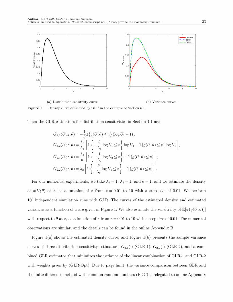
Figure 1 Density curve estimated by GLR in the example of Section 5.1.
Then the GLR estimators for distribution sensitivities in Section 4.1 are
G1,1(U ;z, θ) =−1
θ1g(U ;θ)≤ z (logU1 + 1) ,
G1,2(U ;z, θ) =λ2
λ1
[1
− θ
λ1
logU1 ≤ z
logU1−1g(U ;θ)≤ z logU1
],
G2,1(U ;z, θ) =λ1
θ
[1
− 1
λ2
logU2 ≤ z−1g(U ;θ)≤ z
],
G2,2(U ;z, θ) = λ2
[1
− θ
λ1
logU1 ≤ z−1g(U ;θ)≤ z
].
For our numerical experiments, we take λ1 = 1, λ2 = 1, and θ = 1, and we estimate the density
of g(U ;θ) at z, as a function of z from z = 0.01 to 10 with a step size of 0.01. We perform
106 independent simulation runs with GLR. The curves of the estimated density and estimated
variances as a function of z are given in Figure 1. We also estimate the sensitivity of E[ϕ(g(U ;θ))]
with respect to θ at z, as a function of z from z = 0.01 to 10 with a step size of 0.01. The numerical
observations are similar, and the details can be found in the online Appendix B.
Figure 1(a) shows the estimated density curve, and Figure 1(b) presents the sample variance
curves of three distribution sensitivity estimators: G2,1(·) (GLR-1), G2,2(·) (GLR-2), and a com-
bined GLR estimator that minimizes the variance of the linear combination of GLR-1 and GLR-2
with weights given by (GLR-Opt). Due to page limit, the variance comparison between GLR and
the finite difference method with common random numbers (FDC) is relegated to online Appendix
Author: GLR with Uniform Random Numbers24 Article submitted to Operations Research; manuscript no. (Please, provide the manuscript number!)
0.1 0.2 0.3 0.4 0.5 0.6 0.7 0.8 0.90.5
1
1.5
2
2.5
3
3.5
4q
ua
ntile
va
lue
(a) Confidence intervals for quantiles.
0.1 0.2 0.3 0.4 0.5 0.6 0.7 0.8 0.90.897
0.898
0.899
0.9
0.901
0.902
0.903
0.904
0.905
Co
ve
rag
e r
ate
(b) Coverage rates of confidence intervals.
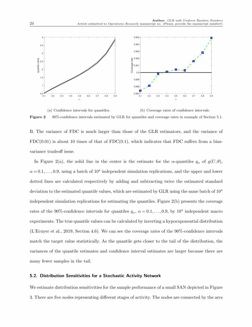
Figure 2 90%-confidence intervals estimated by GLR for quantiles and coverage rates in example of Section 5.1.
B. The variance of FDC is much larger than those of the GLR estimators, and the variance of
FDC(0.01) is about 10 times of that of FDC(0.1), which indicates that FDC suffers from a bias-
variance tradeoff issue.
In Figure 2(a), the solid line in the center is the estimate for the α-quantiles qα of g(U ;θ),
α= 0.1, . . . ,0.9, using a batch of 104 independent simulation replications, and the upper and lower
dotted lines are calculated respectively by adding and subtracting twice the estimated standard
deviation to the estimated quantile values, which are estimated by GLR using the same batch of 104
independent simulation replications for estimating the quantiles. Figure 2(b) presents the coverage
rates of the 90%-confidence intervals for quantiles qα, α= 0.1, . . . ,0.9, by 104 independent macro
experiments. The true quantile values can be calculated by inverting a hypoexponential distribution
(L’Ecuyer et al., 2019, Section 4.6). We can see the coverage rates of the 90%-confidence intervals
match the target value statistically. As the quantile gets closer to the tail of the distribution, the
variances of the quantile estimates and confidence interval estimates are larger because there are
many fewer samples in the tail.
5.2. Distribution Sensitivities for a Stochastic Activity Network
We estimate distribution sensitivities for the sample performance of a small SAN depicted in Figure
3. There are five nodes representing different stages of activity. The nodes are connected by the arcs
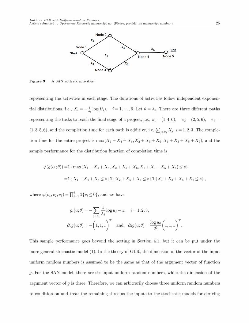
Author: GLR with Uniform Random NumbersArticle submitted to Operations Research; manuscript no. (Please, provide the manuscript number!) 25
Figure 3 A SAN with six activities.
representing the activities in each stage. The durations of activities follow independent exponen-
tial distributions, i.e., Xi =− 1λi
log(Ui), i= 1, . . . ,6. Let θ = λ6. There are three different paths
representing the tasks to reach the final stage of a project, i.e., π1 = (1,4,6), π2 = (2,5,6), π3 =
(1,3,5,6), and the completion time for each path is additive, i.e,∑
j∈πiXj, i= 1,2,3. The comple-
tion time for the entire project is max(X1 +X4 +X6,X2 +X5 +X6,X1 +X3 +X5 +X6), and the
sample performance for the distribution function of completion time is
ϕ(g(U ;θ)) =1max(X1 +X4 +X6,X2 +X5 +X6,X1 +X3 +X5 +X6)≤ z
=1X1 +X4 +X6 ≤ z1X2 +X5 +X6 ≤ z1X1 +X3 +X5 +X6 ≤ z ,
where ϕ(v1, v2, v3) =∏3
i=1 1vi ≤ 0, and we have
gi(u;θ) =−∑j∈πi
1
λjloguj − z, i= 1,2,3,
∂zg(u;θ) =−(
1,1,1
)Tand ∂θg(u;θ) =
logu6
θ2
(1,1,1
)T.
This sample performance goes beyond the setting in Section 4.1, but it can be put under the
more general stochastic model (1). In the theory of GLR, the dimension of the vector of the input
uniform random numbers is assumed to be the same as that of the argument vector of function
g. For the SAN model, there are six input uniform random numbers, while the dimension of the
argument vector of g is three. Therefore, we can arbitrarily choose three uniform random numbers
to condition on and treat the remaining three as the inputs to the stochastic models for deriving
Author: GLR with Uniform Random Numbers26 Article submitted to Operations Research; manuscript no. (Please, provide the manuscript number!)
0 5 10 15
z
0
0.05
0.1
0.15
0.2
0.25S
en
sitiv
ity v
alu
e
(a) Density curve.
0 5 10 15
z
0
0.02
0.04
0.06
0.08
0.1
0.12
0.14
0.16
0.18
Var
ianc
e
(b) Variance curves.
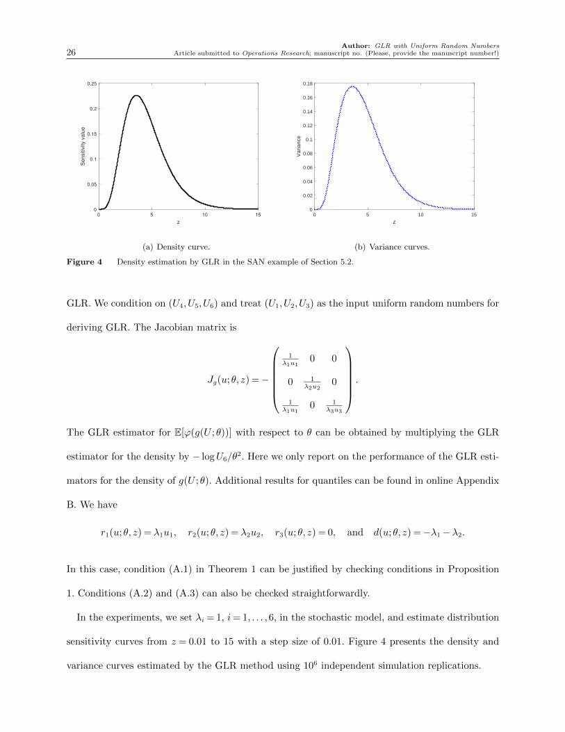
Figure 4 Density estimation by GLR in the SAN example of Section 5.2.
GLR. We condition on (U4,U5,U6) and treat (U1,U2,U3) as the input uniform random numbers for
deriving GLR. The Jacobian matrix is
Jg(u;θ, z) =−
1
λ1u10 0
0 1λ2u2
0
1λ1u1
0 1λ3u3
.
The GLR estimator for E[ϕ(g(U ;θ))] with respect to θ can be obtained by multiplying the GLR
estimator for the density by − logU6/θ2. Here we only report on the performance of the GLR esti-
mators for the density of g(U ;θ). Additional results for quantiles can be found in online Appendix
B. We have
r1(u;θ, z) = λ1u1, r2(u;θ, z) = λ2u2, r3(u;θ, z) = 0, and d(u;θ, z) =−λ1−λ2.
In this case, condition (A.1) in Theorem 1 can be justified by checking conditions in Proposition
1. Conditions (A.2) and (A.3) can also be checked straightforwardly.
In the experiments, we set λi = 1, i= 1, . . . ,6, in the stochastic model, and estimate distribution
sensitivity curves from z = 0.01 to 15 with a step size of 0.01. Figure 4 presents the density and
variance curves estimated by the GLR method using 106 independent simulation replications.
Author: GLR with Uniform Random NumbersArticle submitted to Operations Research; manuscript no. (Please, provide the manuscript number!) 27
5.3. Sensitivities of Control Charts
We estimate sensitivities of the expectations in the numerator and denominator of (12) for control
charts with respect to upper control limit θ = θ2 discussed in Section 4.2. When the system is in
control, the output sample is assumed to follow a uniform distribution on [−1,1] and we define
Zi = 2Ui−1. When the system is out of control, the output sample is assumed to follow a uniform
distribution on [0,2] and we define Zi = 2Ui. Then the transition function of the Markov chain is
Xi = (1−α)Xi−1 +α
θ2− θ1
[1i < χ/∆(2Ui− 1) +1i≥ χ/∆2Ui− θ1] ,
and the weight functions in the GLR estimator are
ri(u;θ) =− 1
θ2− θ1
[1i < χ/∆
(ui−
1
2
)+1i≥ χ/∆ui−
θ1
2
],
d(u;θ) =n
θ2− θ1
.
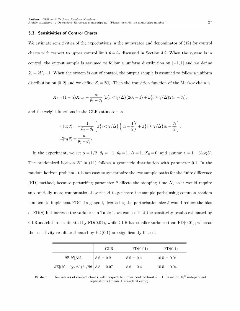
In the experiment, we set α= 1/2, θ1 =−1, θ2 = 1, ∆ = 1, X0 = 0, and assume χ= 1 + 3 logU .
The randomized horizon N ′ in (11) follows a geometric distribution with parameter 0.1. In the
random horizon problem, it is not easy to synchronize the two sample paths for the finite difference
(FD) method, because perturbing parameter θ affects the stopping time N , so it would require
substantially more computational overhead to generate the sample paths using common random
numbers to implement FDC. In general, decreasing the perturbation size δ would reduce the bias
of FD(δ) but increase the variance. In Table 1, we can see that the sensitivity results estimated by
GLR match those estimated by FD(0.01), while GLR has smaller variance than FD(0.01), whereas
the sensitivity results estimated by FD(0.1) are significantly biased.
GLR FD(0.01) FD(0.1)
∂E[N ]/∂θ 8.6 ± 0.2 8.6 ± 0.4 10.5 ± 0.04
∂E[(N −dχ/∆e)+]/∂θ 8.8 ± 0.07 8.6 ± 0.4 10.5 ± 0.04
Table 1 Derivatives of control charts with respect to upper control limit θ= 1, based on 106 independentreplications (mean ± standard error).
Author: GLR with Uniform Random Numbers28 Article submitted to Operations Research; manuscript no. (Please, provide the manuscript number!)
5.4. Sensitivities of Collateralized Debt Obligations
We estimate the sensitivity with respect to the parameter θ that governs the dependence in the
copula model for the expectation of the loss absorbed by the tranche that covers the first 30% of
the total losses for 10 assets if there are defaults, i.e., L− = 0 and L+ = 0.3× (∑10
i=1Li). We set
r = 0.1 and T = 1. The marginal distributions of the defaults are assumed to be exponential, so
τi =− 1λi
log(Xi), i= 1, . . . ,10. The parameters λi and loss Li, i= 1, . . . , n, are randomly generated
from the uniform distribution over (0,1) in the experiments.
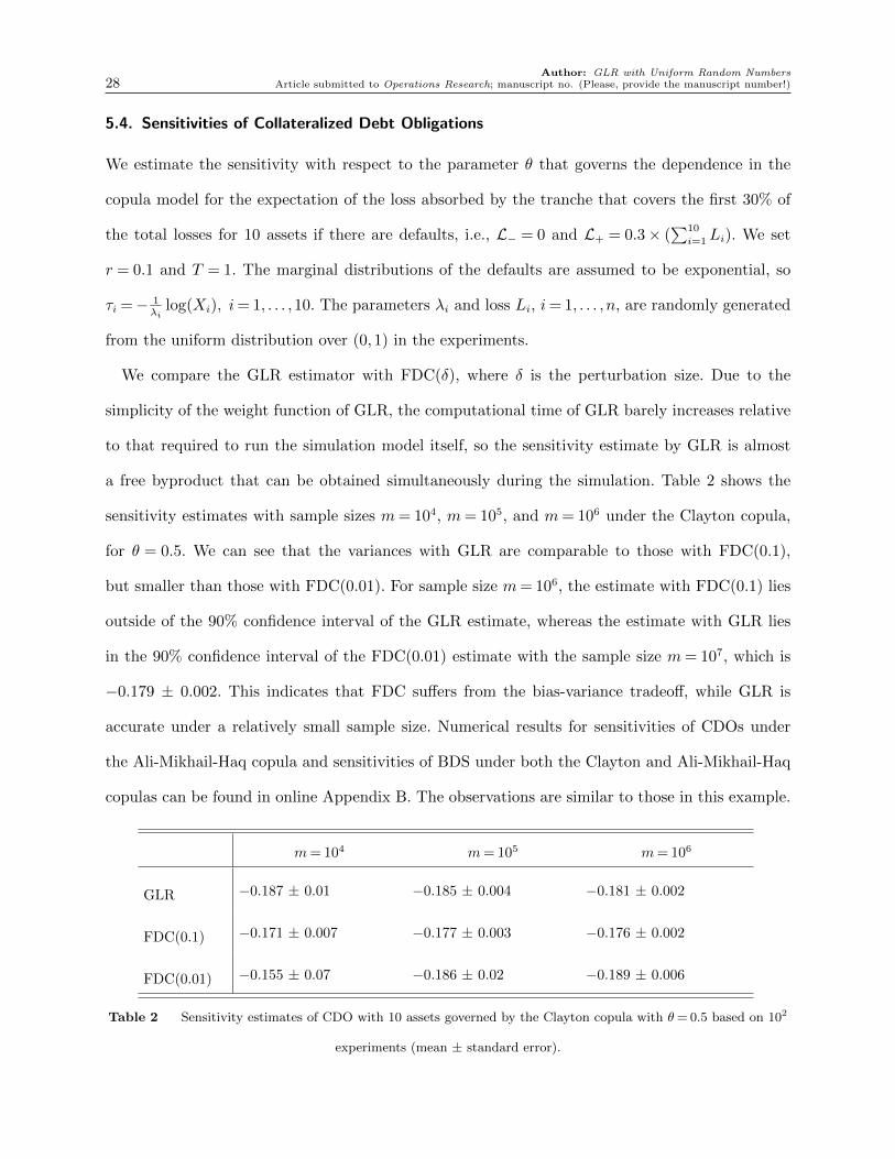
We compare the GLR estimator with FDC(δ), where δ is the perturbation size. Due to the
simplicity of the weight function of GLR, the computational time of GLR barely increases relative
to that required to run the simulation model itself, so the sensitivity estimate by GLR is almost
a free byproduct that can be obtained simultaneously during the simulation. Table 2 shows the
sensitivity estimates with sample sizes m= 104, m= 105, and m= 106 under the Clayton copula,
for θ = 0.5. We can see that the variances with GLR are comparable to those with FDC(0.1),
but smaller than those with FDC(0.01). For sample size m= 106, the estimate with FDC(0.1) lies
outside of the 90% confidence interval of the GLR estimate, whereas the estimate with GLR lies
in the 90% confidence interval of the FDC(0.01) estimate with the sample size m= 107, which is
−0.179 ± 0.002. This indicates that FDC suffers from the bias-variance tradeoff, while GLR is
accurate under a relatively small sample size. Numerical results for sensitivities of CDOs under
the Ali-Mikhail-Haq copula and sensitivities of BDS under both the Clayton and Ali-Mikhail-Haq
copulas can be found in online Appendix B. The observations are similar to those in this example.
m= 104 m= 105 m= 106
GLR −0.187 ± 0.01 −0.185 ± 0.004 −0.181 ± 0.002
FDC(0.1) −0.171 ± 0.007 −0.177 ± 0.003 −0.176 ± 0.002
FDC(0.01) −0.155 ± 0.07 −0.186 ± 0.02 −0.189 ± 0.006
Table 2 Sensitivity estimates of CDO with 10 assets governed by the Clayton copula with θ= 0.5 based on 102
experiments (mean ± standard error).

Author: GLR with Uniform Random NumbersArticle submitted to Operations Research; manuscript no. (Please, provide the manuscript number!) 29
6. Conclusions
In this paper, a GLR method is proposed for a family of stochastic models with uniform random
numbers as inputs. The framework studied in this work covers a large range of discontinuities, and
it includes many applications such as density estimation, and sensitivity analysis for statistical
quality control and credit risk financial derivatives. Since uniform random numbers are the basic
building blocks for generating other random variables, our new method significantly relaxes the
limitations on the input random variables in Peng et al. (2018) and Peng et al. (2020a). The
technical conditions for justifying unbiasedness of GLR are relatively easy to satisfy in practice,
and we show how to verify them on illustrative examples. Ongoing work includes combining GLR
with randomized quasi-Monte Carlo methods and CMC.
AcknowledgmentsThis work was supported in part by the National Natural Science Foundation of China (NSFC) under
Grants 71901003, 71720107003, 71690232, 91846301, 71790615, by the National Science Foundation (NSF)
under Grant CMMI-1434419, by Discovery Grant RGPIN-2018-05795 from NSERC-Canada, and by the Key
Research and Development Program of Beijing Municipal Science and Technology Commission.
References
Asmussen, Søren, Peter W. Glynn. 2007. Stochastic Simulation: Algorithms and Analysis, vol. 57.
Springer.
Bashyam, Sridhar, Michael C. Fu. 1998. Optimization of (s, S) inventory systems with random
lead times and a service level constraint. Management Science 44(12-part-2) S243–S256.
Broadie, Mark, Paul Glasserman. 1996. Estimating security price derivatives using simulation.
Management Science 42(2) 269–285.
Chen, Nan, Yanchu Liu. 2014. American option sensitivities estimation via a generalized infinites-
imal perturbation analysis approach. Operations Research 62(3) 616–632.
Chen, Zhiyong, Paul Glasserman. 2008. Sensitivity estimates for portfolio credit derivatives using
Monte Carlo. Finance and Stochastics 12(4) 507–540.
Cui, Zhenyu, Michael C. Fu, Jian-Qiang Hu, Yanchu Liu, Yijie Peng, Lingjiong Zhu. 2020. Technical
note–On the variance of single-run unbiased stochastic derivative estimators. INFORMS Journal
on Computing 32(2) 390–407.
Embrechts, Paul, Filip Lindskog, Alexander McNeil. 2003. Modelling dependence with copulas
and applications to risk management. S. Rachev, ed., Handbook of Heavy Tailed Distributions
in Finance. Elsevier, 329–384. Chapter 8.
Author: GLR with Uniform Random Numbers30 Article submitted to Operations Research; manuscript no. (Please, provide the manuscript number!)
Fu, Michael C. 1994. Sample path derivatives for (s, S) inventory systems. Operations Research
42(2) 351–364.
Fu, Michael C. 2015. Stochastic gradient estimation, Fu, Michael C. ed. Handbook of Simulation
Optimization, vol. 216. Springer, 105–147. Chapter 5.
Fu, Michael C., L. Jeff Hong, Jian-Qiang Hu. 2009a. Conditional Monte Carlo estimation of quantile
sensitivities. Management Science 55(12) 2019–2027.
Fu, Michael C., Jian-Qiang Hu. 1993. Second derivative sample path estimators for the GI/G/m
queue. Management Science 39(3) 359–383.
Fu, Michael C., Jian-Qiang Hu. 1995. Sensitivity analysis for Monte Carlo simulation of option
pricing. Probability in the Engineering and Informational Sciences 9(3) 417–446.
Fu, Michael C., Jian-Qiang Hu. 1997. Conditional Monte Carlo: Gradient Estimation and Opti-
mization Applications. Kluwer Academic Publishers, Boston.
Fu, Michael C., Jian-Qiang Hu. 1999. Efficient design and sensitivity analysis of control charts
using Monte Carlo simulation. Management Science 45(3) 395–413.
Fu, Michael C., Shreevardhan Lele, Thomas W. M. Vossen. 2009b. Conditional Monte Carlo
gradient estimation in economic design of control limits. Production and Operations Management
18(1) 60–77.
Glasserman, Paul. 1991. Gradient Estimation via Perturbation Analysis. Kluwer Academic Pub-
lishers, Boston.
Glasserman, Paul, Zongjian Liu. 2010. Sensitivity estimates from characteristic functions. Opera-
tions Research 58(6) 1611–1623.
Glynn, Peter W. 1987. Likelihood ratio gradient estimation: an overview. Proceedings of the 1987
Winter Simulation Conference. ACM, 366–375.
Glynn, Peter W. 1990. Likelihood ratio gradient estimation for stochastic systems. Communications
of the ACM 33(10) 75–84.
Glynn, Peter W., Pierre L’Ecuyer. 1995. Likelihood ratio gradient estimation for stochastic recur-
sions. Advances in applied probability 27(4) 1019–1053.
Glynn, Peter W., Yijie Peng, Michael C. Fu, Jianqiang Hu. 2020. Computing sensitivities for
distortion risk measures. submitted to INFORMS Journal on Computing, under third review .
Gong, Wei-Bo, Yu-Chi Ho. 1987. Smoothed perturbation analysis of discrete event dynamical
systems. IEEE Transactions on Automatic Control 32(10) 858–866.
Hammersley, John M., D. C. Handscomb. 1964. Monte Carlo Methods. Methuen, London.
Heidergott, Bernd. 1999. Optimisation of a single-component maintenance system: a smoothed
perturbation analysis approach. European Journal of Operational Research 119(1) 181–190.
Heidergott, Bernd, Taoying Farenhorst-Yuan. 2010. Gradient estimation for multicomponent main-
tenance systems with age-replacement policy. Operations Research 58(3) 706–718.

Author: GLR with Uniform Random NumbersArticle submitted to Operations Research; manuscript no. (Please, provide the manuscript number!) 31
Heidergott, Bernd, Haralambie Leahu. 2010. Weak differentiability of product measures. Mathe-
matics of Operations Research 35(1) 27–51.
Heidergott, Bernd, Felisa J. Vazquez-Abad. 2009. Gradient estimation for a class of systems
with bulk services (a problem in public transportation). ACM Transactions on Modeling and
Computer Simulation 19(3) 13.
Heidergott, Bernd, Warren Volk-Makarewicz. 2016. A measure-valued differentiation approach to
sensitivity analysis of quantiles. Mathematics of Operations Research 41(1) 293–317.
Ho, Yu-Chi, Xi-Ren Cao. 1991. Discrete Event Dynamic Systems and Perturbation Analysis.
Kluwer Academic Publishers, Boston, MA.
Hong, L. Jeff. 2009. Estimating quantile sensitivities. Operations Research 57(1) 118–130.
Hong, L. Jeff, Sandeep Juneja, Jun Luo. 2014. Estimating sensitivities of portfolio credit risk using
Monte Carlo. INFORMS Journal on Computing 26(4) 848–865.
Hong, L Jeff, Guangwu Liu. 2009. Simulating sensitivities of conditional value at risk. Management
Science 55(2) 281–293.
Jiang, Guangxin, Michael C. Fu. 2015. Technical note — On estimating quantile sensitivities via
infinitesimal perturbation analysis. Operations Research 63(2) 435–441.
L’Ecuyer, Pierre. 1990. A unified view of the IPA, SF, and LR gradient estimation techniques.
Management Science 36(11) 1364–1383.
L’Ecuyer, Pierre, Peter W. Glynn. 1994. Stochastic optimization by simulation: Convergence proofs
for the GI/G/1 queue in steady-state. Management Science 40(11) 1562–1578.
L’Ecuyer, Pierre, Florian Puchhammer, Amal Ben Abdellah. 2019. Monte Carlo and quasi-Monte
Carlo density estimation via conditioning. arXiv preprint arXiv:1906.04607 .
Lei, Lei, Yijie Peng, Michael C. Fu, Jian-Qiang Hu. 2018. Applications of generalized likelihood
ratio method to distribution sensitivities and steady-state simulation. Journal of Discrete Event
Dynamic Systems 28(1) 109–125.
Lei, Lei, Yijie Peng, Michael C. Fu, Jian-Qiang Hu. 2020. Sensitivity analysis of portfolio
credit derivatives by conditional Monte Carlo simulation. preprint in ResearchGate with DOI:
10.13140/RG.2.2.21951.97444 .
Li, David. 2000. On default correlation: a copula approach. Journal of Fixed Income 9 43–54.
Liu, Guangwu, L. Jeff Hong. 2011. Kernel estimation of the Greeks for options with discontinuous
payoffs. Operations Research 59(1) 96–108.
Marshall, Albert W., Ingram Olkin. 1988. Families of multivariate distributions. Journal of the
American Statistical Association 83(403) 834–841.
Mohamed, Shakir, Mihaela Rosca, Michael Figurnov, Andriy Mnih. 2020. Monte Carlo gradient
estimation in machine learning. forthcoming in Journal of Machine Learning Research .
Author: GLR with Uniform Random Numbers32 Article submitted to Operations Research; manuscript no. (Please, provide the manuscript number!)
Nakayama, Marvin K. 2014. Confidence intervals for quantiles using sectioning when applying
variance-reduction techniques. ACM Transactions on Modeling and Computer Simulation 24(4)
1–21.
Nelsen, Roger B. 2006. An Introduction to Copulas, vol. 139. 2nd ed. Springer Science & Business
Media.
Peng, Yijie, Michael C Fu, Peter W Glynn, Jian-Qiang Hu. 2017. On the asymptotic analysis of
quantile sensitivity estimation by Monte Carlo simulation. Proceedings of Winter Simulation
Conference 2336–2347.
Peng, Yijie, Michael C Fu, Bernd Heidergott, Henry Lam. 2020a. Maximum likelihood estimation
by Monte Carlo simulation: Towards data-driven stochastic modeling. Operations Research,
forthcoming .
Peng, Yijie, Michael C. Fu, Jian-Qiang Hu. 2016. On the regularity conditions and applications for
generalized likelihood ratio method. Proceedings of Winter Simulation Conference. IEEE Press,
919–930.
Peng, Yijie, Michael C. Fu, Jian-Qiang Hu, Bernd Heidergott. 2018. A new unbiased stochastic
derivative estimator for discontinuous sample performances with structural parameters. Opera-
tions Research 66(2) 487–499.
Peng, Yijie, Li Xiao, Bernd Heidergott, Jeff Hong, Henry Lam. 2020b. Stochastic gradient estima-
tion for artificial neural networks. submitted to INFORMS Journal on Computing, under second
review .
Pflug, Georg Ch. 1988. Derivatives of probability measures-concepts and applications to the opti-
mization of stochastic systems. Pravin Varaiya, Alexander B. Kurzhanski, eds., Discrete Event
Systems: Models and Applications. Springer Berlin Heidelberg, Berlin, Heidelberg, 252–274.
Rhee, Chang-han, Peter W. Glynn. 2015. Unbiased estimation with square root convergence for
SDE models. Operations Research 63(5) 1026–1043.
Rubinstein, Reuven Y., Alexander Shapiro. 1993. Discrete Event Systems: Sensitivity Analysis and
Stochastic Optimization by the Score Function Method . Wiley, New York.
Serfling, Robert J. 1980. Approximation Theorems of Mathematical Statistics. Wiley.
Sklar, A. 1959. Fonctions de repartition a n dimensions et leurs marges. Publications de l’Institut
de Statistique de l’Universite de Paris 8 229–231.
Suri, Rajan, Michael A. Zazanis. 1988. Perturbation analysis gives strongly consistent sensitivity
estimates for the M/G/1 queue. Management Science 34(1) 39–64.
Wang, Yongqiang, Michael C. Fu, Steven I. Marcus. 2012. A new stochastic derivative estimator
for discontinuous payoff functions with application to financial derivatives. Operations Research
60(2) 447–460.