Embed Size (px)
Citation preview
HAL Id: hal-00858299https://hal.archives-ouvertes.fr/hal-00858299
Submitted on 5 Sep 2013
HAL is a multi-disciplinary open accessarchive for the deposit and dissemination of sci-entific research documents, whether they are pub-lished or not. The documents may come fromteaching and research institutions in France orabroad, or from public or private research centers.
L’archive ouverte pluridisciplinaire HAL, estdestinée au dépôt et à la diffusion de documentsscientifiques de niveau recherche, publiés ou non,émanant des établissements d’enseignement et derecherche français ou étrangers, des laboratoirespublics ou privés.
Higher-Order Sliding Mode Control for LateralDynamics of Autonomous Vehicles, with Experimental
ValidationGilles Tagne, Reine Talj, Ali Charara
To cite this version:Gilles Tagne, Reine Talj, Ali Charara. Higher-Order Sliding Mode Control for Lateral Dynamics ofAutonomous Vehicles, with Experimental Validation. IEEE Intelligent Vehicles Symposium (IV 2013),Jun 2013, Gold Coast, Australia. pp.678-683, 2013. <hal-00858299>
Higher-Order Sliding Mode Control for Lateral Dynamics ofAutonomous Vehicles, with Experimental Validation
Gilles Tagne, Reine Talj and Ali Charara
Abstract— This paper presents design and experimental val-idation of a vehicle lateral controller for autonomous vehiclebased on a higher-order sliding mode control. We used thesuper-twisting algorithm to minimize the lateral displacementof the autonomous vehicle with respect to a given referencetrajectory. The control input is the steering angle and theoutput is the lateral displacement error. The particularity ofsuch a strategy is to take advantage of the robustness of thesliding mode controller against nonlinearities and parametricuncertainties in the model, while reducing chattering, themain drawback of first order sliding mode. To validate thecontrol strategy, the closed-loop system simulated on Matlab-Simulink has been compared to the experimental data acquiredon our vehicle DYNA, a Peugeot 308, according to severaldriving scenarios. The validation shows robustness and goodperformance of the proposed control approach.
I. INTRODUCTION
Technological advances in recent years have favored theemergence of intelligent vehicles with the capacity to an-ticipate and compensate a failure (of driver, vehicle orinfrastructure) or even to ensure an autonomous driving.
The ”DARPA Grand Challenge” (2004, 2005) and the”DARPA Urban Challenge” (2007) [1], organized by theDefense Advanced Research Projects Agency (DARPA) ofthe U.S. has stimulated research for the development ofautonomous vehicles. This is an area of growing research.One of the major challenges today is to ensure autonomousdriving at high speed.
An autonomous driving can be divided in three steps:• The perception of the environment. It consists on detect-
ing road, obstacles and other vehicles. A vision systemcomposed of sensors like cameras, lasers, radars andGPS is usually used to achieve this goal. It providesa dynamic map of the near environment of the au-tonomous vehicle.
• The trajectory generation. It consists in generating andchoosing one trajectory (reference path) in the navigablespace.
• The vehicle control. It consists to handle vehicle usingactuators like brake, accelerator and steering wheel tofollow the reference path. This step can be divided intotwo tasks: longitudinal control and lateral control.
This paper focus on the third main step, that treat thevehicle control. And more precisely, the lateral control of the
Gilles Tagne, Reine Talj and Ali Charara are working at HeudiasycLaboratory, UMR CNRS 7253, Universite de Technologie de Compiegne,BP 20529, 60205 Compiegne, [email protected], [email protected],[email protected]
intelligent vehicle. Lateral control of an autonomous vehicledeal with automatically steering the vehicle to follow thereference path. It has been studied since the 1950s. Giventhe high nonlinearities of the vehicle system on one hand,and the uncertainties and disturbances of such a system onthe other hand, a very important issue to be considered inthe control design is the robustness. The controller should beable to reject the disturbances caused by wind, coefficient offriction of the road and many other reasons, and able to dealwith parameter uncertainties and variations encountered inautomotive applications. For example, in [2], a recent pre-sentation of Junior; Stanford’s autonomous research vehicle(the second at the DARPA Urban Challenge) is made for thepurpose of ensuring robust autonomous driving.
For over 40 years, considerable research have been con-ducted to provide lateral guidance of autonomous vehicles.Several control strategies have been developed in the lit-erature: In [3], proportional controller is used. In [4], PIcontroller is used. In [5], nested PID controller is proposed.In [6], controller based on state feedback control is devel-oped. In [7], the H∞ control is used. In [8], control byLyapunov stability theory is developed. In [9], a controllerbased on adaptive control is presented. In [10], [11], con-trollers based on linear quadratic optimal predictive controlare developed.
In [12], techniques from artificial intelligence and fuzzylogic are particularly used. These approaches use humansteering skills to improve the automatic driving performance.
In [13], a comparison of a proportional, adaptive, H∞ andfuzzy controllers is presented. This comparison is made usingseveral criteria to evaluate the robustness: variations of cur-vature, speed variations, changes of the friction coefficient ofthe road and disturbances due to wind. From this comparison,it appears that the proportional controller is the one that hasthe biggest errors. H∞ and fuzzy controllers have equivalentperformances. The adaptive controller has the best response.
Model predictive control (MPC) appears to be well suitedto the trajectory following [2], [14]. It allows to consider theproblem of trajectory tracking for nonlinear systems takinginto account the constraints on the state variables and/orcontrol inputs. In addition, this control technique is provedto be robust against system parameter variations. However,for autonomous driving at high speed, the computation time(non-linear optimization algorithms) becomes very large forreal-time operation [10], [14].
Different comparisons showed that the class of adaptivecontrollers represents a very promising technique for suchuncertain and nonlinear application.
The sliding mode control is one of the most promisingcontrol techniques for trajectory tracking. In [15], [16], [17],the first-order sliding mode control is applied to the lateralcontrol. This control strategy is well suited for drivingapplications. It provides constant and small displacementerrors when the speed increases. Also, it allows to obtainexperimental results comparable or better than the linearcontrollers with gain self-adjusting [16]. In addition, it isparticularly suited to compensate for uncertainties (variationsof model parameters) and disturbances encountered in auto-motive applications. This method also has the advantage ofproducing simpler control laws lower complexity comparedto other approaches of robust control [18]. However, theirmain drawback is the chattering. One of the solutions toreduce the chattering is the using of higher-order slidingmode.
We propose in this paper a controller based on higher-order sliding mode, the algorithm of super-twisting to ensurelateral control at high speed of an autonomous vehicle. Theproblem considers that the vehicle is equipped with all thenecessary sensors to measure or estimate lateral acceleration,lateral velocity, yaw rate and steering angle. To validatethe proposed approach, tests were made with real dataacquired by our vehicle DYNA, on the tracks and circuits ofCERAM1. The experimental results show the effectivenessof the proposed approach.
This paper is organized as follows. Sections II presentsthe dynamic models of the vehicle that we used. In SectionIII, we develop our control strategy. Section IV presents theresults and the evaluation of robustness. Section V presentsthe conclusions, remarks and future work directions.
II. DYNAMIC MODELS OF VEHICLE
In this work, we use two vehicle models. The first oneis the bicycle model used in Section III.B for the controldesign. The second is the 4-wheel vehicle model used tovalidate in simulation the proposed control in closed loop.
A. Bicycle model
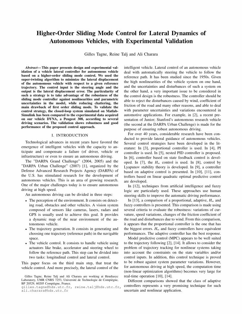
To design the controller, a simple and widely used dy-namic bicycle model [6] is considered. See Fig. 1. This
Fig. 1. Bicycle model
model is used to represent the lateral vehicle behavior (lateralacceleration, yaw rate, sideslip angle) and assumes that the
1CERAM -”Centre d’Essais et de Recherche Automobile de Morte-fontaine” is an automobile testing and research center located in France.
vehicle is symmetrical, and sideslip angles on the same axleare equal. The roll and pitch dynamics are neglected andangles are assumed to be small (steering, sideslip, yaw).
With a linear tire force model we obtain a linear parametervarying model (LPV), the longitudinal velocity Vx is consid-ered as a varying parameter. This LPV model is composedof the lateral and yaw dynamics given by: y =− (C f +Cr)
mVxy− (
L f C f−LrCrmVx
+Vx)ψ +C fm δ
ψ =−L f C f−LrCrIzVx
y−L2
fC f +L2
rCr
IzVxψ +
L f C fIz
δ
(1)
where y and ψ represent respectively the lateral positionand the yaw angle of the vehicle. Table I presents vehiclenomenclature and parameters.
TABLE IVEHICLE NOMENCLATURE AND PARAMETERS (BICYCLE MODEL)
Vx Longitudinal velocity - [m/s]y Lateral velocity - [m/s]ψ Yaw rate - [rad/s]δ steering wheel angle - [rad]m Mass 1719 [kg]Iz Yaw moment of inertia 3300 [kgm2]L f Front axle-COG distance 1.195 [m]Lr Rear axle-COG distance 1.513 [m]C f Cornering stiffness of the front tire 170550 [N/rad]Cr Cornering stiffness of the rear tire 137844 [N/rad]
B. 4-wheel model
To compare our simulation results with experimental data,we used a more representative model. Namely, a 4-wheelmodel to represent the vehicle dynamics, with Dugoff’s tiremodel for logitudinal and lateral forces [19].
III. CONTROL STRATEGY
The sliding mode control (SMC) has been developed since1950s and is recognized as one of the most promisingtechniques for robust control. The principle of SMC is toconstrain the system trajectories to reach in finite time andremain on a sliding surface (see Fig. 2). However, its main
Fig. 2. SMC principle
drawback is the chattering. Three main approaches to theelimination and mitigation of chattering in the SMC havebeen proposed in the mid 1980s [20]:• The use of smooth functions instead of the discontinu-
ous function sign,• The use of an approach based on observers,• The use of higher order sliding mode.

A. Super-twisting algorithm
The super-twisting algorithm is developed to control sys-tems with a relative degree 1, and to ensure robust stabilitywhile reducing chattering (the main drawback of the first-order sliding mode). Consider a system of the form:
x = f (t,x)+g(t,x)u(t) (2)
where u is the control input, x ∈ Rn the state vector, and,f , g continuous functions. We define a sliding variable sof relative degree 1, whose derivative can be expressed asfollows:
s(t,s) = φ(t,s)+ϕ(t,s)u(t) (3)
The aim of the controller is to ensure converge to the slidingsurface defined by s = 0. Only the measurement of s in realtime is required.It is assumed that there exist positive constants s0, bmin, bmax,C0 such that ∀x ∈ Rn and |s(t,x)|< s0 , the system satisfiesthe following conditions: |u(t)| ≤Umax
0 < bmin ≤ |ϕ(t,s)| ≤ bmax|φ(t,s)|<C0
(4)
The sliding mode control algorithm based on super-twintingis given by:
u(t) = u1 +u2
{u1 =−α |s|τ sign(s), τ ∈ ]0, 0.5]u2 =−β sign(s) (5)
with α and β positive constants. The finite time convergenceto the sliding surface is guaranteed by the following condi-tions [21]:
β > C0bmin
α ≥√
4C0(bmaxβ+C0)
b2min(bminβ−C0)
(6)
For more details of the convergence and robustness of thealgorithm, see [22], [23].
B. Application to lateral control of autonomous vehicles
The lateral error dynamics at the center of gravity of thevehicle, with respect to a reference trajectory, is given by:
e = ay−ayre f (7)
where ay and ayre f are the lateral acceleration of the vehicle,and the desired one on the reference trajectory respectively.Assuming that the desired lateral acceleration of the vehiclecan be written as ayre f = V 2
x /R, where R is the radius ofcurvature of the road and given that ay = y+Vxψ , we have:
e = y+Vxψ− V 2x
R(8)
Replacing y by its expression in equation (1), we obtain:
e =− (C f +Cr)
mVxy− L f C f−LrCr
mVxψ− V 2
xR +
C fm δ (9)
The control input is the steering angle and the lateraldisplacement is the output. The objective of the control lawis to cancel the lateral displacement error.
Choosing the sliding variable s as follows:
s = e+λe (10)
we obtain: s = e+ λ e. Replacing e by its expression (11),we obtain:
s =−C f +CrmVx
y− L f C f−LrCrmVx
ψ− V 2xR +
C fm δ +λ e (11)
The variable s has a relative degree r = 1. By identificationwith (3), we have s(t,s) = φ(t,s)+ϕ(t,s)u(t), with:{
φ(t,s) =−C f +CrmVx
y− L f C f−LrCrmVx
ψ− V 2xR +λ e
ϕ(t,s) = C fm
(12)
Applying the super-twisting theorem, the control input canbe defined as follows:
δST = u1 +u2
{u1 =−α |s|1/2 sign(s)u2 =−β sign(s)
(13)
To avoid important peaks in transient phases, we add anequivalent command δeq obtained by solving the equations = 0. This term has the role of a feedforward that approachthe system to the sliding surface, and is given by:
δeq =−mC f
φ(t,s) (14)
Hence, the steering angle representing the control input ofthe system is defined as follows:
δ = δST +δeq (15)
IV. EXPERIMENTAL VALIDATION
The experimental data used here are acquired on the CE-RAM test circuits by our vehicle DYNA (Fig. 3). This vehicleis equipped with several sensors: an Inertial MeasurementUnit (IMU) measuring accelerations (x, y, z) and the yawrate. The CORREVIT for measuring the sideslip angle andlongitudinal velocity. Torque hubs for measuring tire-roadefforts and vertical loads on each tire. Four laser sensors tomeasure the height of the chassis. GPS and a CCD camera.Data provided via the CAN bus of the vehicle are also used,as the steering angle, and the rotational speed of the wheels.
Fig. 3. Experimental vehicle (DYNA)
To validate our control law, we perform several tests of ourvehicle DYNA. The collected data are reference data that willbe compared to those obtained using simulations of the law
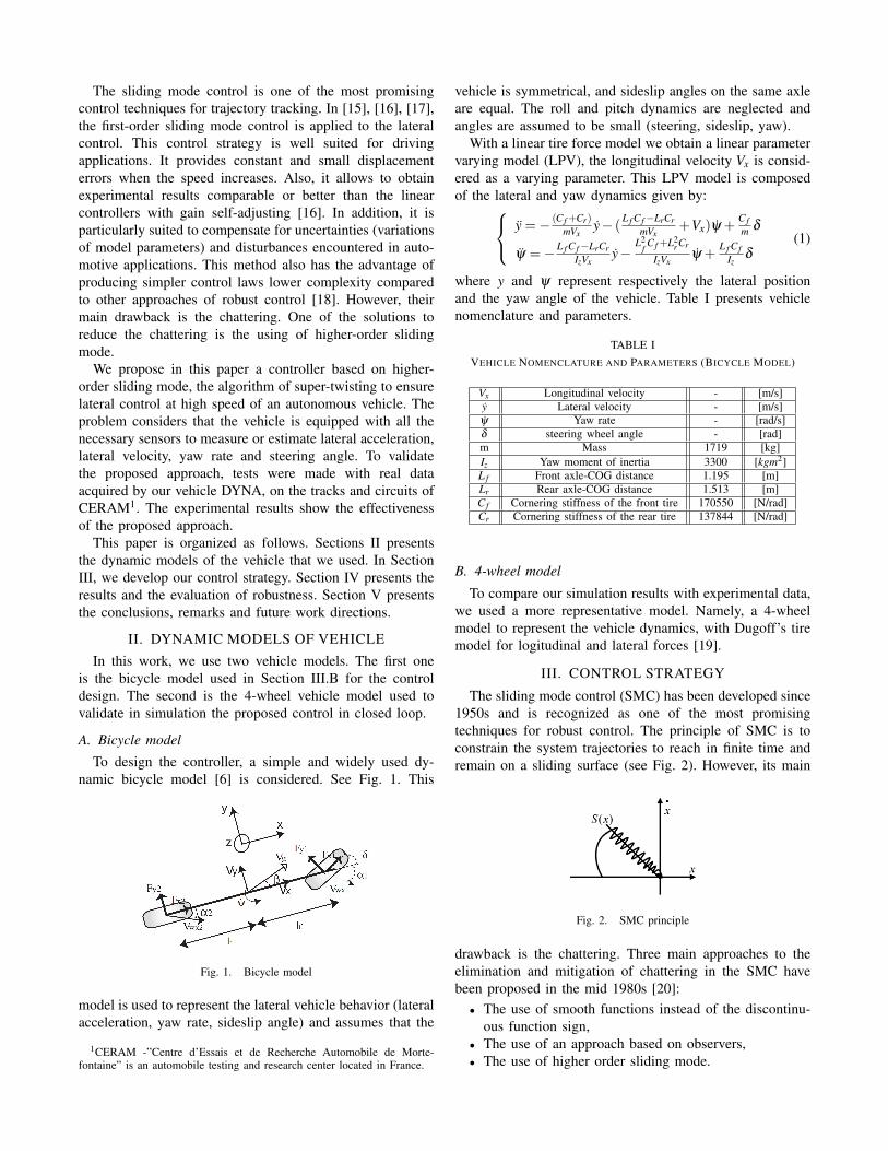
of closed loop control. Simulations were carried out with ourvehicle full model. For the control law, we used λ = 8,α =0.002,β = 0.0001 and the nominal vehicle parameters (seeTable 1). The robustness of the controlled system is evaluatedin terms of changes in parameters (longitudinal speed) anduncertainties encountered in automotive applications.
A. Robustness of the controller during normal driving
The first test (Fig. 4, Fig. 5 and Fig. 6) was carried outwith the goal of verifying the robustness of the controllerduring normal driving. The lateral acceleration is less than4m/s2. Longitudinal velocity is almost constant (13.5m/s)with a variable curvature between −0.02m−1 and 0.09m−1.Fig. 4 shows the longitudinal speed variations. Fig. 5 presents
0 10 20 30 40 50 600
2
4
6
8
10
12
14
Long
itudi
nal s
peed
[m/s
]
Fig. 4. Longitudinal speed
different curves. The reference path and the trajectory fol-lowed by the controlled vehicle. We have also the lateraldeviation and the yaw error. The controlled vehicle is ableto track the reference path with small error under variousconditions. The displacement from the guideline not exceed7.5cm in transient state in this test conditions.Fig. 6 presents dynamic variables of vehicle: the steeringangle, the yaw rate and the lateral acceleration. We comparereal data with data given by the simulated closed-loopsystem. Dynamic variables are very close to measured ones.The steering angle is smooth and the steering error does notexceed 1.7 degrees (comparing the measurement). Measuredyaw rate is very close to the one obtained in simulation. Wenote the appearance of a small offset after the great turning.This is due to the non-linearity caused by the large steering.In this scenario, although the assumption of small angles is
not respected (the steering angle is greater than 12 degreeswhile turning), the controller is able to follow the path withlow error. This first simulation shows the good performanceand robustness of the controller.
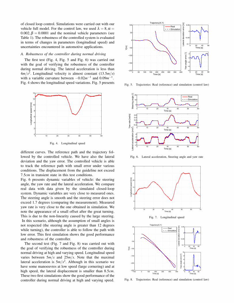
The second test (Fig. 7 and Fig. 8) was carried out withthe goal of verifying the robustness of the controller duringnormal driving at high and varying speed. Longitudinal speedvaries between 5m/s and 25m/s. Note that the maximallateral acceleration is 5m/s2. Although in this scenario wehave some manoeuvres at low speed (large cornering) and athigh speed, the lateral displacement is smaller than 8.5cm.These two first simulations show the good performance of thecontroller during normal driving at high and varying speed.
0 50 100 150 200 250 300 350 400−200
−150
−100
−50
0
50
100Trajectory(X,Y)
Time [s]
Y[m
]
RealSimulation
0 20 40 60−0.1
−0.05
0
0.05
Late
ral d
evia
tion
erro
r [m
]
Time [s]
0 20 40 60−6
−4
−2
0
2
Yaw
ang
le e
rror
[°]
Time [s]
Fig. 5. Trajectories: Real (reference) and simulation (control law)
0 10 20 30 40 50 60
0
10
20
Ste
erin
g an
gle
[°]
Time [s]
RealSimulation
0 10 20 30 40 50 60
−0.2
0
0.2
0.4
0.6
Yaw
rat
e [r
ad/s
]Time [s]
0 10 20 30 40 50 60−4
−2
0
2
4La
tera
l acc
eler
atio
n [m
/s2 ]
Time [s]
Fig. 6. Lateral acceleration, Steering angle and yaw rate
0 10 20 30 40 50 60 700
5
10
15
20
25
30
Long
itudi
nal s
peed
[m/s
]
Time [s]
Fig. 7. Longitudinal speed
−100 0 100 200 300 400 500−250
−200
−150
−100
−50
0
50Trajectory(X,Y)
Time [s]
Y[m
]
RealSimulation
0 20 40 60−0.1
−0.05
0
0.05
Late
ral d
evia
tion
erro
r [m
]
Time [s]
0 20 40 600
2
4
6
8
10
Yaw
ang
le e
rror
[°]
Time [s]
Fig. 8. Trajectories: Real (reference) and simulation (control law)
B. Robustness of the controller to strong nonlinear dynamics
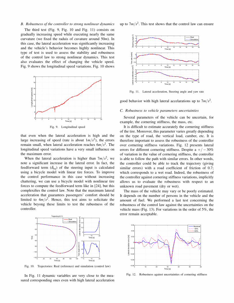
The third test (Fig. 9, Fig. 10 and Fig. 11) consists ongradually increasing speed while executing nearly the samecurvature (we fixed the raduis of cuvature around 50m). Inthis case, the lateral acceleration was significantly increasingand the vehicle’s behavior becomes highly nonlinear. Thistype of test is used to assess the stability and robustnessof the control law to strong nonlinear dynamics. This testalso evaluates the effect of changing the vehicle speed.Fig. 9 shows the longitudinal speed variations. Fig. 10 shows
0 2 4 6 8 10 12 14 16 18 206
8
10
12
14
16
18
20
Long
itudi
nal s
peed
[m/s
]
Time [s]
Fig. 9. Longitudinal speed
that even when the lateral acceleration is high and thelarge increasing of speed (rate is about 1m/s2), the errorsremain small, when lateral acceleration reaches 6m/s2. Thelongitudinal speed variations have a very small influence onthe maximum error.
When the lateral acceleration is higher than 7m/s2, wenote a significant increase in the lateral error. In fact, thefeedforward term (δeq) of the steering input is calculatedusing a bicycle model with linear tire forces. To improvethe control performance in this case without increasingchattering, we can use a bicycle model with nonlinear tireforces to compute the feedforward term like in [24], but thiscomplexifies the control law. Note that the maximum lateralacceleration that guarantees passengers’ comfort should belimited to 4m/s2. Hence, this test aims to solicitate thevehicle beyong these limits to test the rubustness of thecontroller.
0 20 40 60 80 100 120−120
−100
−80
−60
−40
−20
0
20Trajectory(X,Y)
Time [s]
Y[m
]
RealSimulation
0 10 20
0
0.2
0.4
0.6
Late
ral d
evia
tion
erro
r [m
]
Time [s]
0 10 20−0.5
0
0.5
1
1.5
Yaw
ang
le e
rror
[°]
Time [s]
Fig. 10. Trajectories: Real (reference) and simulation (control law)
In Fig. 11 dynamic variables are very close to the mea-sured corresponding ones even with high lateral acceleration
up to 7m/s2. This test shows that the control law can ensure
0 2 4 6 8 10 12 14 16 18 20−6
−4
−2
0
2
Ste
erin
g an
gle
[°]
Time [s]
RealSimulation
0 2 4 6 8 10 12 14 16 18 20
−0.4
−0.2
0
Yaw
rat
e [r
ad/s
]
Time [s]
0 2 4 6 8 10 12 14 16 18 20−8
−6
−4
−2
0
2
Late
ral a
ccél
erat
ion
[m/s
2 ]
Time [s]
Fig. 11. Lateral acceleration, Steering angle and yaw rate
good behavior with high lateral accelarations up to 7m/s2.
C. Robustness to vehicle parameters uncertainties
Several parameters of the vehicle can be uncertain, forexample, the cornering stiffness, the mass, etc.
It is difficult to estimate accurately the cornering stiffnessof the tire. Moreover, this parameter varies greatly dependingon the type of road, the vertical load, camber, etc. It istherefore important to assess the robustness of the controllerover cornering stiffness variations. Fig. 12 presents lateralerrors for different cornering stiffness. Despite a +/−30%of variation in the value of cornering stiffness, the controlleris able to follow the path with similar errors. In other words,the controller could be able to track the trajectory (givingsimilar errors) with a road coefficient of friction of 0.7;which corresponds to a wet road. Indeed, the robustness ofthe controller against cornering stiffness variations, implicitlyallows us to evaluate the robustness with respect to anunknown road pavement (dry or wet).
The mass of the vehicle may vary or be poorly estimated.It depends on the number of persons in the vehicle and theamount of fuel. We performed a last test concerning therobustness of the control law against the uncertainties on thevehicle mass (Fig. 13). For variations in the order of 5%, theerror remain acceptable.
0 10 20 30 40 50 60−0.08
−0.06
−0.04
−0.02
0
0.02
0.04
0.06
Late
ral d
evia
tion
erro
r [m
]
Time [s]
Nominal−30%+30%
Fig. 12. Robustness against uncertainties of cornering stiffness
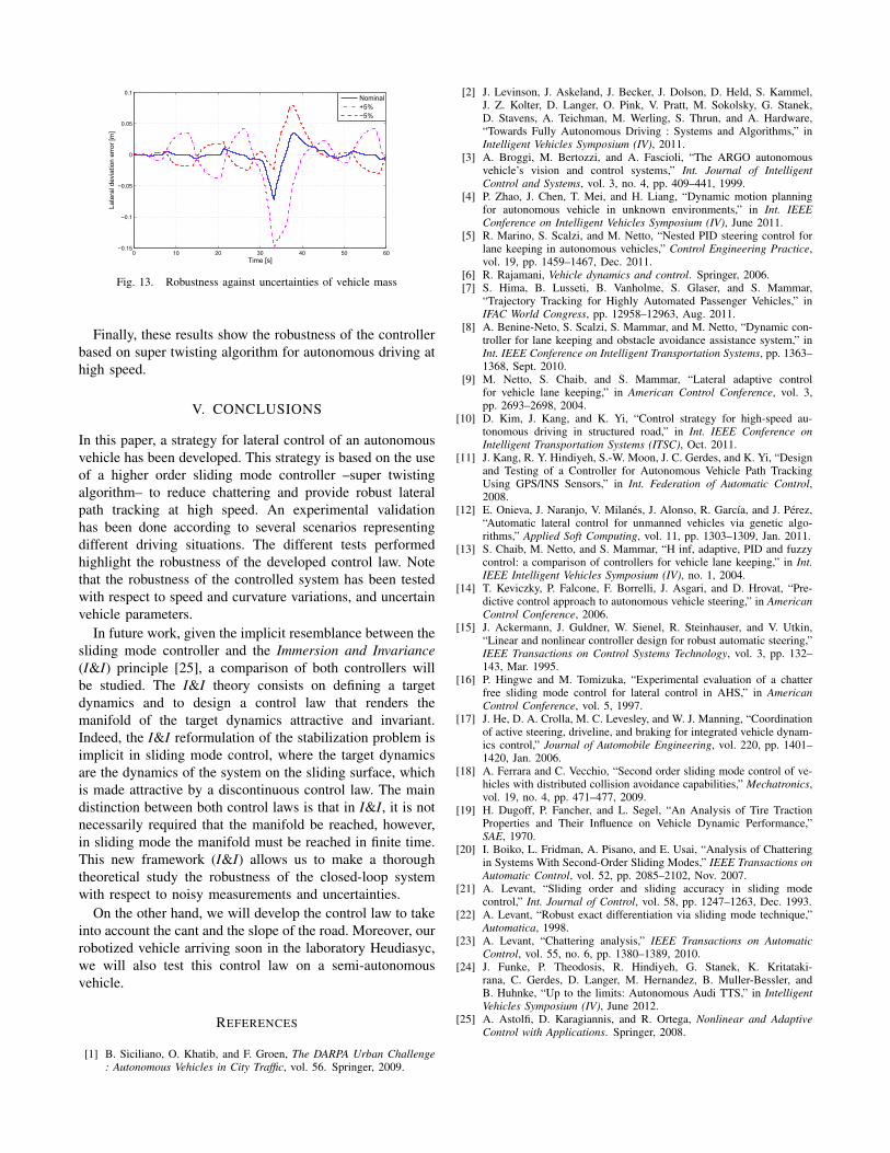
0 10 20 30 40 50 60−0.15
−0.1
−0.05
0
0.05
0.1
Late
ral d
evia
tion
erro
r [m
]
Time [s]
Nominal+5%−5%
Fig. 13. Robustness against uncertainties of vehicle mass
Finally, these results show the robustness of the controllerbased on super twisting algorithm for autonomous driving athigh speed.
V. CONCLUSIONS
In this paper, a strategy for lateral control of an autonomousvehicle has been developed. This strategy is based on the useof a higher order sliding mode controller –super twistingalgorithm– to reduce chattering and provide robust lateralpath tracking at high speed. An experimental validationhas been done according to several scenarios representingdifferent driving situations. The different tests performedhighlight the robustness of the developed control law. Notethat the robustness of the controlled system has been testedwith respect to speed and curvature variations, and uncertainvehicle parameters.
In future work, given the implicit resemblance between thesliding mode controller and the Immersion and Invariance(I&I) principle [25], a comparison of both controllers willbe studied. The I&I theory consists on defining a targetdynamics and to design a control law that renders themanifold of the target dynamics attractive and invariant.Indeed, the I&I reformulation of the stabilization problem isimplicit in sliding mode control, where the target dynamicsare the dynamics of the system on the sliding surface, whichis made attractive by a discontinuous control law. The maindistinction between both control laws is that in I&I, it is notnecessarily required that the manifold be reached, however,in sliding mode the manifold must be reached in finite time.This new framework (I&I) allows us to make a thoroughtheoretical study the robustness of the closed-loop systemwith respect to noisy measurements and uncertainties.
On the other hand, we will develop the control law to takeinto account the cant and the slope of the road. Moreover, ourrobotized vehicle arriving soon in the laboratory Heudiasyc,we will also test this control law on a semi-autonomousvehicle.
REFERENCES
[1] B. Siciliano, O. Khatib, and F. Groen, The DARPA Urban Challenge: Autonomous Vehicles in City Traffic, vol. 56. Springer, 2009.
[2] J. Levinson, J. Askeland, J. Becker, J. Dolson, D. Held, S. Kammel,J. Z. Kolter, D. Langer, O. Pink, V. Pratt, M. Sokolsky, G. Stanek,D. Stavens, A. Teichman, M. Werling, S. Thrun, and A. Hardware,“Towards Fully Autonomous Driving : Systems and Algorithms,” inIntelligent Vehicles Symposium (IV), 2011.
[3] A. Broggi, M. Bertozzi, and A. Fascioli, “The ARGO autonomousvehicle’s vision and control systems,” Int. Journal of IntelligentControl and Systems, vol. 3, no. 4, pp. 409–441, 1999.
[4] P. Zhao, J. Chen, T. Mei, and H. Liang, “Dynamic motion planningfor autonomous vehicle in unknown environments,” in Int. IEEEConference on Intelligent Vehicles Symposium (IV), June 2011.
[5] R. Marino, S. Scalzi, and M. Netto, “Nested PID steering control forlane keeping in autonomous vehicles,” Control Engineering Practice,vol. 19, pp. 1459–1467, Dec. 2011.
[6] R. Rajamani, Vehicle dynamics and control. Springer, 2006.[7] S. Hima, B. Lusseti, B. Vanholme, S. Glaser, and S. Mammar,
“Trajectory Tracking for Highly Automated Passenger Vehicles,” inIFAC World Congress, pp. 12958–12963, Aug. 2011.
[8] A. Benine-Neto, S. Scalzi, S. Mammar, and M. Netto, “Dynamic con-troller for lane keeping and obstacle avoidance assistance system,” inInt. IEEE Conference on Intelligent Transportation Systems, pp. 1363–1368, Sept. 2010.
[9] M. Netto, S. Chaib, and S. Mammar, “Lateral adaptive controlfor vehicle lane keeping,” in American Control Conference, vol. 3,pp. 2693–2698, 2004.
[10] D. Kim, J. Kang, and K. Yi, “Control strategy for high-speed au-tonomous driving in structured road,” in Int. IEEE Conference onIntelligent Transportation Systems (ITSC), Oct. 2011.
[11] J. Kang, R. Y. Hindiyeh, S.-W. Moon, J. C. Gerdes, and K. Yi, “Designand Testing of a Controller for Autonomous Vehicle Path TrackingUsing GPS/INS Sensors,” in Int. Federation of Automatic Control,2008.
[12] E. Onieva, J. Naranjo, V. Milanes, J. Alonso, R. Garcıa, and J. Perez,“Automatic lateral control for unmanned vehicles via genetic algo-rithms,” Applied Soft Computing, vol. 11, pp. 1303–1309, Jan. 2011.
[13] S. Chaib, M. Netto, and S. Mammar, “H inf, adaptive, PID and fuzzycontrol: a comparison of controllers for vehicle lane keeping,” in Int.IEEE Intelligent Vehicles Symposium (IV), no. 1, 2004.
[14] T. Keviczky, P. Falcone, F. Borrelli, J. Asgari, and D. Hrovat, “Pre-dictive control approach to autonomous vehicle steering,” in AmericanControl Conference, 2006.
[15] J. Ackermann, J. Guldner, W. Sienel, R. Steinhauser, and V. Utkin,“Linear and nonlinear controller design for robust automatic steering,”IEEE Transactions on Control Systems Technology, vol. 3, pp. 132–143, Mar. 1995.
[16] P. Hingwe and M. Tomizuka, “Experimental evaluation of a chatterfree sliding mode control for lateral control in AHS,” in AmericanControl Conference, vol. 5, 1997.
[17] J. He, D. A. Crolla, M. C. Levesley, and W. J. Manning, “Coordinationof active steering, driveline, and braking for integrated vehicle dynam-ics control,” Journal of Automobile Engineering, vol. 220, pp. 1401–1420, Jan. 2006.
[18] A. Ferrara and C. Vecchio, “Second order sliding mode control of ve-hicles with distributed collision avoidance capabilities,” Mechatronics,vol. 19, no. 4, pp. 471–477, 2009.
[19] H. Dugoff, P. Fancher, and L. Segel, “An Analysis of Tire TractionProperties and Their Influence on Vehicle Dynamic Performance,”SAE, 1970.
[20] I. Boiko, L. Fridman, A. Pisano, and E. Usai, “Analysis of Chatteringin Systems With Second-Order Sliding Modes,” IEEE Transactions onAutomatic Control, vol. 52, pp. 2085–2102, Nov. 2007.
[21] A. Levant, “Sliding order and sliding accuracy in sliding modecontrol,” Int. Journal of Control, vol. 58, pp. 1247–1263, Dec. 1993.
[22] A. Levant, “Robust exact differentiation via sliding mode technique,”Automatica, 1998.
[23] A. Levant, “Chattering analysis,” IEEE Transactions on AutomaticControl, vol. 55, no. 6, pp. 1380–1389, 2010.
[24] J. Funke, P. Theodosis, R. Hindiyeh, G. Stanek, K. Kritataki-rana, C. Gerdes, D. Langer, M. Hernandez, B. Muller-Bessler, andB. Huhnke, “Up to the limits: Autonomous Audi TTS,” in IntelligentVehicles Symposium (IV), June 2012.
[25] A. Astolfi, D. Karagiannis, and R. Ortega, Nonlinear and AdaptiveControl with Applications. Springer, 2008.