Embed Size (px)
Citation preview

U.S. Department of Energy
NREL is a national laboratory of the U.S. Department of Energy Office of Energy Efficiency & Renewable Energy Operated by the Alliance for Sustainable Energy, LLC This report is available at no cost from the National Renewable Energy Laboratory (NREL) at www.nrel.gov/publications.
Contract No. DE-AC36-08GO28308
High-Penetration PV Integration Handbook for Distribution Engineers Rich Seguin, Jeremy Woyak, David Costyk, and Josh Hambrick Electrical Distribution Design
Barry Mather National Renewable Energy Laboratory
Technical Report NREL/TP-5D00-63114 January 2016
NREL is a national laboratory of the U.S. Department of Energy Office of Energy Efficiency & Renewable Energy Operated by the Alliance for Sustainable Energy, LLC This report is available at no cost from the National Renewable Energy Laboratory (NREL) at www.nrel.gov/publications.
Contract No. DE-AC36-08GO28308
National Renewable Energy Laboratory 15013 Denver West Parkway Golden, CO 80401 303-275-3000 • www.nrel.gov
High-Penetration PV Integration Handbook for Distribution Engineers Rich Seguin, Jeremy Woyak, David Costyk, and Josh Hambrick Electrical Distribution Design
Barry Mather National Renewable Energy Laboratory
Prepared under Task No. SS12.2930
Technical Report NREL/TP-5D00-63114 January 2016
NOTICE
This report was prepared as an account of work sponsored by an agency of the United States government. Neither the United States government nor any agency thereof, nor any of their employees, makes any warranty, express or implied, or assumes any legal liability or responsibility for the accuracy, completeness, or usefulness of any information, apparatus, product, or process disclosed, or represents that its use would not infringe privately owned rights. Reference herein to any specific commercial product, process, or service by trade name, trademark, manufacturer, or otherwise does not necessarily constitute or imply its endorsement, recommendation, or favoring by the United States government or any agency thereof. The views and opinions of authors expressed herein do not necessarily state or reflect those of the United States government or any agency thereof.
This report is available at no cost from the National Renewable Energy Laboratory (NREL) at www.nrel.gov/publications.
Available electronically at SciTech Connect http:/www.osti.gov/scitech
Available for a processing fee to U.S. Department of Energy and its contractors, in paper, from:
U.S. Department of Energy Office of Scientific and Technical Information P.O. Box 62 Oak Ridge, TN 37831-0062 OSTI http://www.osti.gov Phone: 865.576.8401 Fax: 865.576.5728 Email: [email protected]
Available for sale to the public, in paper, from:
U.S. Department of Commerce National Technical Information Service 5301 Shawnee Road Alexandria, VA 22312 NTIS http://www.ntis.gov Phone: 800.553.6847 or 703.605.6000 Fax: 703.605.6900 Email: [email protected]
Cover Photos by Dennis Schroeder: (left to right) NREL 26173, NREL 18302, NREL 19758, NREL 29642, NREL 19795.
NREL prints on paper that contains recycled content.
iii
This report is available at no cost from the National Renewable Energy Laboratory (NREL) at www.nrel.gov/publications
Acknowledgments This work was supported by the U.S. Department of Energy under Contract No. DOE-EE0002061 with the National Renewable Energy Laboratory. The authors thank Dr. Ranga Pitchumani, Alvin Razon and Kevin Lynn for their present or past support of the NREL/SCE High-Penetration PV Integration Project. The authors would also like to thank the California Solar Initiative (CSI) RD&D Program and Program Manager Itron, namely Anne Peterson and Stephan Barsun, for past support of the NREL/SCE Hi-Penetration PV Integration Project that provided for a broader analysis of high-penetration PV circuits than otherwise would have been possible. Thanks are due to Southern California Edison (SCE) for their long-term support of the project and for providing circuit models, operational data, and access to real-world sets of distribution systems on which the findings of the project are summarized in this handbook. The information included in this handbook, and the general scope of the handbook, was steered and edited by a select number of distribution engineering experts formally organized into the Distribution Energineering Review Committee (DERC). The DERC members were:
Dr. Thomas McDermott P.E. – University of Pittsburgh Steve Steffel P.E. – Pepco Holdings Inc. Phuong Tran – Lakeland Electric Hawk Asgerisson P.E. – DTE Energy Sylvester Toe P.E. – Georgia Power Franco Bruno – Central Hudson Gas and Electric Araya Gebeyehu P.E. – Southern California Edison
In addition to those listed above, the staff members working on PV interconnection at some of the above utilities also reviewed drafts of the handbook. All the comments and edits from the experts in the DERC and their staff members were instrumental in keeping the information contained in and the scope of this handbook relevant to practicing distribution engineers. Thanks to the DERC and other reviewers for their time and effort reviewing drafts of the handbook. Finally, thanks are due to the other team members and collaborator in the NREL/SCE High-Penetration PV Integration Project. While this Handbook can’t possibly show the whole extent of the research completed under the auspices of the project all such work was critical in producing a better understanding of the impacts of high-penetration PV integration on the distribution system and how to determine and mitigate those impacts. Thanks to Quanta Technology, Clean Power Research, Satcon Technology Corp. and the Florida State University Center for Advanced Power Systems.
iv
This report is available at no cost from the National Renewable Energy Laboratory (NREL) at www.nrel.gov/publications
List of Acronyms AC alternating current DC direct current DG distributed generation DTT direct transfer trip IEEE Institute of Electrical and Electronics Engineers ITIC Information Technology Industry Council LTC load tap changer PF power factor POI point of interconnection PV photovoltaic SCADA supervisory control and data acquisition TOV temporary overvoltage VRT voltage regulating transformer
v
This report is available at no cost from the National Renewable Energy Laboratory (NREL) at www.nrel.gov/publications
Table of Contents 1 Introduction ........................................................................................................................................... 1
1.1 Background on the NREL/SCE Hi-Pen Project ............................................................................ 1 1.2 Intended Use of this Handbook ..................................................................................................... 3 1.3 Organization of the Handbook ...................................................................................................... 3
2 High-Penetration PV Distribution-Level Impacts .............................................................................. 4 2.1 Introduction ................................................................................................................................... 4 2.2 Overload-Related Impacts ............................................................................................................. 4
2.2.1 Ampacity Ratings ............................................................................................................. 4 2.2.2 Masked Load .................................................................................................................... 5 2.2.3 Cold Load Pickup ............................................................................................................. 5
2.3 Voltage-Related Impacts ............................................................................................................... 6 2.3.1 Feeder Voltage Profile ..................................................................................................... 6 2.3.2 Overvoltage ...................................................................................................................... 6 2.3.3 Potential for Increased Substation Voltage ...................................................................... 7 2.3.4 Flicker .............................................................................................................................. 7 2.3.5 Automatic Voltage Regulation Equipment ...................................................................... 8
2.4 Reverse Power Flow Impacts ...................................................................................................... 10 2.4.1 Substation and Bulk System Impacts ............................................................................. 10 2.4.2 Temporary and Transient Overvoltage ........................................................................... 10 2.4.3 Automatic Voltage Regulation Equipment .................................................................... 12
2.5 System Protection Impacts .......................................................................................................... 13 2.5.1 Fault Current and Interrupting Rating ............................................................................ 13 2.5.2 Fault Sensing .................................................................................................................. 14 2.5.3 Desensitizing the Substation Relay ................................................................................ 15 2.5.4 Line-to-Ground Utility System Overvoltage .................................................................. 16 2.5.5 Nuisance Fuse Blowing .................................................................................................. 17 2.5.6 Reclosing Out of Synchronism ...................................................................................... 18 2.5.7 Islanding ......................................................................................................................... 18 2.5.8 Sectionalizer Miscount ................................................................................................... 19 2.5.9 Reverse Power Relay Operation—Malfunctions on Secondary Networks .................... 19 2.5.10 Reverse Power Relay Operation—Substation ................................................................ 20 2.5.11 Cold Load Pickup With and Without PV ....................................................................... 20 2.5.12 Faults Within a PV Zone ................................................................................................ 22 2.5.13 Isolating PV for an Upstream Fault ................................................................................ 23 2.5.14 Fault Causing Voltage Sag and Tripping PV ................................................................. 23 2.5.15 Distribution Automation Studies and Reconfiguration .................................................. 23
2.6 Circuit Configurations ................................................................................................................. 24 2.6.1 Normal System Configuration ....................................................................................... 24 2.6.2 Abnormal System Configuration ................................................................................... 24 2.6.3 Future/Planned System Configurations .......................................................................... 24 2.6.4 Contingency Conditions ................................................................................................. 25
3 Model-Based Study Guide for Assessing PV Impacts.................................................................... 27 3.1 Introduction ................................................................................................................................. 27 3.2 Develop a Base Case Model ........................................................................................................ 29
3.2.1 Distribution Circuit Models ........................................................................................... 30 3.2.2 PV System Models ......................................................................................................... 37
3.3 Time Series Input—Develop Data Used to Inform the Models .................................................. 40 3.3.1 Utility SCADA Data (Synchronizing Data and Navigating the Issues) ......................... 40 3.3.2 Modeled PV Power Output Data (with existing PV Plant Data) .................................... 41
vi
This report is available at no cost from the National Renewable Energy Laboratory (NREL) at www.nrel.gov/publications
3.3.3 Clear-Sky Calculated PV Power Output Data ................................................................ 42 3.4 Validate Time Series Measurement Data .................................................................................... 43
3.4.1 Validate Circuit Model ................................................................................................... 43 3.4.2 Add Measurements ......................................................................................................... 43 3.4.3 Run Power Flow ............................................................................................................. 43
3.5 Determine Quasi-Steady-State Critical Time Points and Study Criteria ..................................... 43 3.5.1 Identify Critical Time Points .......................................................................................... 44 3.5.2 Choose Study Criteria .................................................................................................... 44
3.6 Analyze and Assess PV Impact ................................................................................................... 44 3.6.1 Assess PV Using Power Flow Analysis ......................................................................... 47 3.6.2 Assess PV Using Fault Analysis .................................................................................... 48
3.7 Porterville Example—PV Assessment ........................................................................................ 49 3.7.1 Developing the System Model ....................................................................................... 51 3.7.2 Assessing PV Using Power Flow Analysis—Example 1 ............................................... 52 3.7.3 Assessing PV Using Fault Analysis—Example 1 .......................................................... 60 3.7.4 Assessing PV Using Power Flow Analysis—Example 2 ............................................... 62 3.7.5 Assessing PV Using Fault Analysis—Example 2 .......................................................... 67
4 Mitigation Techniques for High-Penetration PV Impacts ............................................................... 71 4.1 Introduction ................................................................................................................................. 71 4.2 Mitigation Techniques Supported by PV Inverter Capabilities .................................................. 71
4.2.1 Constant Power Factor Operation .................................................................................. 71 4.2.2 Other Advanced PV Controls ......................................................................................... 72
4.3 Mitigation Techniques to Alleviate PV Impacts ......................................................................... 74 4.3.1 Steady-State Voltage Impacts ........................................................................................ 74 4.3.2 Dynamic Voltage Impacts .............................................................................................. 75 4.3.3 Reverse Power Flow Impacts ......................................................................................... 76 4.3.4 Overload Impacts ........................................................................................................... 77 4.3.5 System Protection Impacts ............................................................................................. 77
4.4 Porterville Example—Constant Power Factor Operation ........................................................... 80 4.5 Additional Advanced Inverter Techniques .................................................................................. 82
4.5.1 Power Factor Scheduling ............................................................................................... 82 4.5.2 Reactive Power Compensation or Constant VAR Operation ......................................... 82 4.5.3 Active Volt/VAR Control or Dynamic Voltage Control ................................................ 83
4.6 Selecting a Mitigation Technique ................................................................................................ 86 References ................................................................................................................................................. 88 Appendix A: Review and Fix Bad Data ................................................................................................... 90
Discover Bad Data ................................................................................................................................ 90 Tabular Format ............................................................................................................................ 90 SQL Queries Within Access........................................................................................................ 92
Ignore Bad Data .................................................................................................................................... 93 Correct Bad Data .................................................................................................................................. 94
Correct Data Using SQL Queries Within Access ........................................................................ 95 Correct Data Using Excel ............................................................................................................ 95
Appendix B: Criteria for Evaluating PV Generation Impacts ................................................................ 96
vii
This report is available at no cost from the National Renewable Energy Laboratory (NREL) at www.nrel.gov/publications
List of Figures Figure 2.1. Masked load—difference between measured load and native load on a peak load day (Mather
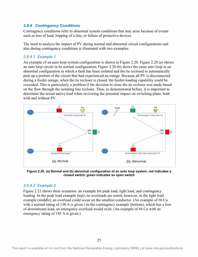
et al. 2014)................................................................................................................................ 5 Figure 2.2. Impact of solar PV on the voltage profile of a feeder ................................................................. 7 Figure 2.3. Impact of solar PV on voltage compensation provided by line drop compensation. ................. 9 Figure 2.4. Peak load voltage profiles—PV compared to no PV .................................................................. 9 Figure 2.5. Example of TOV due to load rejection (Nelson et al. 2015) .................................................... 11 Figure 2.6. Example of transient overvoltage ............................................................................................. 11 Figure 2.7. Runaway voltage regulator ....................................................................................................... 13 Figure 2.8. Impact of PV on fuse interruption ratings ................................................................................ 14 Figure 2.9. Impact of PV on breaker interruption ratings ........................................................................... 14 Figure 2.10. PV may desensitize protection devices to faults ..................................................................... 15 Figure 2.11. Reduction in fault current through substation relay because of PV ....................................... 16 Figure 2.12. PV may cause line-to-ground overvoltage ............................................................................. 17 Figure 2.13. Illustration of nuisance fuse-blowing caused by large PV penetration .................................. 18 Figure 2.14. Reclosing out of synchronism ................................................................................................ 18 Figure 2.15. Illustration of sectionalizer miscount because of PV.............................................................. 19 Figure 2.16. Reverse power relay operation because of PV ....................................................................... 20 Figure 2.17. Time-varying characteristic of cold load (Lawhead at el. 2006) ............................................ 22 Figure 2.18. PV may be isolated for an upstream fault ............................................................................... 23 Figure 2.19. Reconfiguration in the presence of PV ................................................................................... 24 Figure 2.20. (a) Normal and (b) abnormal configuration of an auto loop system, red indicates a closed
switch, green indicates an open switch .................................................................................. 25 Figure 2.21. Overload during normal and contingency conditions ............................................................. 26 Figure 3.1. Flowchart for model development ............................................................................................ 28 Figure 3.2. Flowchart for performing PV impact studies ........................................................................... 29 Figure 3.3. (Left) Detailed and (right) simplified models of distribution substations ................................ 31 Figure 3.4. Example of voltage regulators and control details ................................................................... 32 Figure 3.5. Example of voltage regulator compensation ............................................................................ 33 Figure 3.6. Representative capacitor bank control and timing parameters ................................................. 34 Figure 3.7. Calculating the native load ....................................................................................................... 36 Figure 3.8. PV impact study flowchart ....................................................................................................... 46 Figure 3.9. DEW’s DER automated assessment application dialog ........................................................... 50 Figure 3.10. Map of the Porterville circuit .................................................................................................. 51 Figure 3.11. Porterville overhead capacitor control used for voltage regulation ........................................ 52 Figure 3.12. Scenario 1—worst-case study criteria violations for critical load days .................................. 53 Figure 3.13. Porterville example study results—flicker associated with sudden loss and return of rated PV
at POI ..................................................................................................................................... 55 Figure 3.14. Porterville example study results—capacitor switching compared to percentage loss of
PV .......................................................................................................................................... 56 Figure 3.15. Porterville example study results—flicker associated with sudden loss and return of rated PV
at the POI compared to the fixed absorbing power factor ...................................................... 57 Figure 3.16. Porterville example study results—capacitor switching compared to loss of rated PV with
fixed absorbing power factor ................................................................................................. 58 Figure 3.17. Porterville example study results—5-MW PV site radiant variability analysis by minute .... 59 Figure 3.18. Porterville example study results—5-MW PV site radiant variability analysis by hour ........ 59 Figure 3.19. Porterville example study results—detailed fault assessment of the circuit ........................... 61 Figure 3.20. Porterville example study results—circuit breaker desensitizing with PV ............................. 62 Figure 3.21. Single-line diagram of the circuit section used for the transient overvoltage study ............... 63 Figure 3.22. Voltage across line charging capacitance ............................................................................... 67
viii
This report is available at no cost from the National Renewable Energy Laboratory (NREL) at www.nrel.gov/publications
Figure 4.1. Porterville example study results—flicker associated with sudden loss and return of rated PV at the POI compared to the fixed absorbing power factor ...................................................... 82
Figure 4.2. Example of reactive droop curve with dead band .................................................................... 83 Figure 4.3. Schematic of the 8,500-node test feeder reduced to include only the primary circuit (Mather
et al. 2014).............................................................................................................................. 84 Figure 4.4. Comparison of voltages at PV POIs when PV systems are operating with different control
strategies (Mather et al. 2014) ................................................................................................ 85 Figure 4.5. Comparison of voltages at Load 3 and Load 6 when PV systems use different control
strategies (Mather et al. 2014) ................................................................................................ 86 Figure 4.6. Reactive power of the PV systems for various control strategies (Mather et al. 2014) ............ 86
List of Tables Table 3.1. PV Generation Data Resources .................................................................................................. 42 Table 3.2. Sample DER Impact Study Criteria ........................................................................................... 44 Table 3.3. Porterville Example Study Results—Variability for 2011......................................................... 60 Table 3.4. Porterville Example Study Results—Worst-Case Fault Analysis ............................................. 60 Table 3.5. Parameters for the Circuit Section Shown in Figure 3.21 .......................................................... 65 Table 3.6. Initial Conditions and Pre-Islanding Inverter Currents .............................................................. 66 Table 3.7. Substation Impedance ................................................................................................................ 68 Table 3.8. Relay Settings ............................................................................................................................ 68 Table 3.9. Fault Currents at the Substation ................................................................................................. 68 Table 3.10. Fault Currents at the Location of West PV Provided by the Substation .................................. 69 Table 3.11. Fault Currents at the Location of East PV Provided by the Substation ................................... 69 Table 3.12. Fault Current at the Switch ...................................................................................................... 69 Table 4.1. Voltage at the Point of Common Coupling and Corresponding Clearing Time ........................ 76
1
This report is available at no cost from the National Renewable Energy Laboratory (NREL) at www.nrel.gov/publications
1 Introduction 1.1 Background on the NREL/SCE Hi-Pen Project This handbook has been developed as part of a five-year research project which began in 2010. The National Renewable Energy Laboratory (NREL), Southern California Edison (SCE), Quanta Technology, Satcon Technology Corporation, Electrical Distribution Design (EDD), and Clean Power Research (CPR) teamed together to analyze the impacts of high-penetration levels of photovoltaic (PV) systems interconnected onto the SCE distribution system. This project was designed specifically to leverage the experience that SCE and the project team would gain during the significant installation of 500 MW of commercial scale PV systems (1-5 MW typically) starting in 2010 and completing in 2015 within SCE’s service territory through a program approved by the California Public Utility Commission (CPUC). The research objectives of this project included the following:
Development of distribution and PV system models required to evaluate the impacts of high-penetration PV
Identification and development of the necessary distribution system studies and analysis appropriate for determining the impacts of high-penetration PV
Development of high-penetration PV impact mitigation strategies in the form of advanced inverter functions to enable high-penetration PV interconnection
Lab testing of advanced PV inverter functions
Field testing of advanced PV inverter functions
Development of a handbook for high-penetration PV grid integration that is useful to distribution system engineers facing the integration of high-penetrations of PV into their service territories.
Many of the above objectives and their resulting research outcomes have informed the development of this handbook which directly correlates to the last research objective listed above. This handbook is not inclusive of all the research outcomes of the project. For further reading on the project and its research results please see the following select publications:
B. Mather, B. Kroposki, R. Neal, F. Katiraei, A. Yazdani, J. R. Aguero, T. E. Hoff, B. L. Norris, A. Parkins, R. Seguin, C. Schauder, Southern California Edison High-Penetration Photovoltaic Project – Year 1, NREL Technical Report, TP-5500-50875, June, 2011.
B. Mather, R. Neal, Integrating High Penetrations of PV into Southern California: Year 2 Project Update, proc. of IEEE Photovoltaic Specialists Conference, Austin, TX, June, 2012.
B. Mather, M. Kromer, L. Casey, Advanced Photovoltaic Inverter Functionality Verification using 500 kW Power Hardware-in-Loop (PHIL) Complete System Laboratory Testing, in proc. of IEEE Innovative Smart Grid Technology Conference, Washington, DC, Feb., 2013.
2
This report is available at no cost from the National Renewable Energy Laboratory (NREL) at www.nrel.gov/publications
F. Katiraei, D. Paradis, B. Mather, Comparative Analysis of Time-Series Studies and Transient Simulations for Impact Assessment of PV Integration on Reduced IEEE 8500 Node Test Feeder, proc. of IEEE Power and Energy Society General Meeting, Vancouver, BC, Canada, July, 2013.
B. Mather, S. Shah, B. Norris, J. Dise, L. Yu, D. Paradis, F. Katiraei, R. Seguin, D. Costyk, J. Woyak, J. Jung, K. Russel, R. Broadwater, NREL/SCE High Penetration PV Integration Project: FY13 Annual Report, NREL Technical Report, TP-5D00-61269, June, 2014.
B. Mather, S. Shah, In Divergence There is Strength, IEEE Power and Energy Magazine, March/April, 2015.
B. Mather, A. Gebeyehu, Field Demonstration of Using Advanced PV Inverter Functionality to Mitigate the Impacts of High-Penetration PV Grid Integration on the Distribution System, proc. of IEEE Photovoltaic Specialists Conference, New Orleans, LA, June, 2015.
D. Cheng, B. Mather, R. Seguin, J. Hambrick, PV Impact Assessment for Very High Penetration Levels, proc. of IEEE Photovoltaic Specialists Conference, New Orleans, LA, June, 2015.
F. Katiraei, B. Mather, A. Momeni, L. Yu, G. Sanchez, Field Verification and Data Analysis of High PV Penetration Impacts on Distribution Systems, proc. of IEEE Photovoltaic Specialists Conference, New Orleans, LA, June, 2015.
Most of the above publications and additional publications related to the project are available at no charge from NREL’s publications online database which can be access at:
http://www.nrel.gov/research/publications.html
Additional information on the project – including links to all the project deliverables – is available on the DOE SunShot Grid Performance and Reliability website at:
http://energy.gov/eere/sunshot/grid-performance-and-reliability
Also see the California Solar Initiative’s website for the project at:
http://www.calsolarresearch.org/funded-projects/67-analysis-of-highpenetration-levels-of-pv-into-the-distribution-grid-in-california
The NREL/SCE High-Penetration PV Integration Project was supported by funding from the U.S. Department of Energy (DOE) Solar Program through a competitively awarded grant (DE-FOA-0000085) and through a competitively awarded grant provided by the California Solar Initiative (CSI) RD&D Program – supported by the California Public Utilities Commission and managed by iTron.
3
This report is available at no cost from the National Renewable Energy Laboratory (NREL) at www.nrel.gov/publications
1.2 Intended Use of this Handbook This handbook was developed for practicing distribution system engineers working in North America. The handbook is written to present the potential impacts of high-penetration PV integration, provide model-based analysis approaches for determining the level of PV impact and suggest potential mitigation measures that could be taken to reduce PV impacts to distribution system engineers with a working knowledge of distribution systems planning and operations. While the focused development of the handbook has been distribution system engineers, it is the authors’ hope that this handbook will find as wide a usage as possible potentially including personnel at all positions at a utility, by PV developers, researchers and even energy customers wanting a better understanding of the distribution system.
While the research that produced this handbook was focused on the integration of utility-scale PV system (1-5 MW) much of the information contained in the following pages is also relevant for the integration of large numbers of small PV systems as are found in some residential neighborhoods throughout the country.
1.3 Organization of the Handbook This handbook is organized into four chapters. This chapter introduces the underlying project, which lead to the development of the handbook, as well as the use of the handbook and the organization of the handbook. Chapter 2 presents the various types of distribution-system level impacts which can be a concern when considering the integration of high-penetrations of PV onto a distribution system. Chapter 2 is organized by the impact potentially induced by PV integration as opposed to the specific cause of the impact. The impacts described are: overload, voltage, reverse power flow, protection and circuit configuration. Chapter 3 gives a detailed study process for determining the level of the potential PV impacts presented in Chapter 2. The study process shown covers the entire modeling process – from development of the base case model scenario to completing the analysis necessary to assess PV impacts. The final section of Chapter 3 gives a detailed case study as an example of the proposed PV impact study process. Chapter 4 covers the mitigation measures that can be taken on the distribution-system and using PV inverters, a constituent part of PV systems, to reduce the distribution-system level impacts of high-penetration PV integration. Mitigation measures are organized by PV impact similar to Chapter 2. An example of PV mitigation is included. Two appendices to this handbook, A and B, include information on correcting bad data used in the study process and an example list of PV impact screening thresholds respectively. Appendix B is included as an example of PV impact thresholds only. The specific PV impact thresholds for each distribution utility are likely to be dependent on typical design standards and operation practices.
4
This report is available at no cost from the National Renewable Energy Laboratory (NREL) at www.nrel.gov/publications
2 High-Penetration PV Distribution-Level Impacts 2.1 Introduction Traditionally, the distribution system has been designed to operate in a radial fashion, with flow in one direction from the substation source to the load. Starting with the passage of the Public Utility Regulatory Policies Act in 1978, distributed generation (DG) has begun to appear more frequently on the distribution system. Recently, because of improving economic viability, incentives, public utility commissions requiring the consideration of DG as an alternative to traditional circuit upgrades and state renewable portfolio standards, distributed photovoltaic (PV) systems have become more common. Although distribution engineers are more familiar today with the design and operation challenges posed by DG, high penetrations of PV, which has relatively unpredictable and sometimes highly variable output, represent a less familiar challenge.
Unlike traditional distribution analysis, which is done at a few meaningful time points (e.g., heaviest load), impacts of high penetrations of PV should be investigated using time-varying analysis, which captures the interactions among load, generation, and control equipment that are difficult to predict using a single time point analysis. Time-varying analysis should include the behavior of fast-acting inverters, dynamic loads, and automatic voltage control devices on the feeders.
This chapter documents potential impacts caused by high-penetration PV scenarios. Many definitions of high-penetration PV exist. For the purposes of this handbook, high-penetration PV is defined as the level at which the distribution network has a high likelihood of experiencing voltage, thermal, and/or protection criteria violations.
2.2 Overload-Related Impacts High penetrations of PV systems can cause the ampacity ratings of circuit elements to be exceeded in a number of ways. Perhaps most intuitively, the total generation from attached PV systems can overload circuit elements located between PV systems and load centers on a given circuit. Additionally, PV can mask load that can overload circuit elements if the PV disconnects.
Also, although load is often quite diverse, PV systems located relatively close to each other are generally fairly coincident (depending on their orientation). In such cases, multiple instances of PV systems that are sized to offset the attached load (e.g., in a residential subdivision) may overload circuit elements because of the coincident nature of the peak PV output relative to the diverse nature of the peak load.
When examining overloads, consideration should be given to both normal system conditions and a contingency loss of circuit segments.
2.2.1 Ampacity Ratings The location of PV can significantly impact the loading of feeder sections; therefore, it is necessary to verify that the feeder sections located between the PV and the substation have enough available capacity to distribute the PV’s surplus power (after subtracting local and downstream load). At high penetrations, particularly during light load conditions with high PV output, the line section loading may increase as the PV contribution becomes larger than the
5
This report is available at no cost from the National Renewable Energy Laboratory (NREL) at www.nrel.gov/publications
native base load. The flow in some instances may increase above that of the peak native load (no PV output).
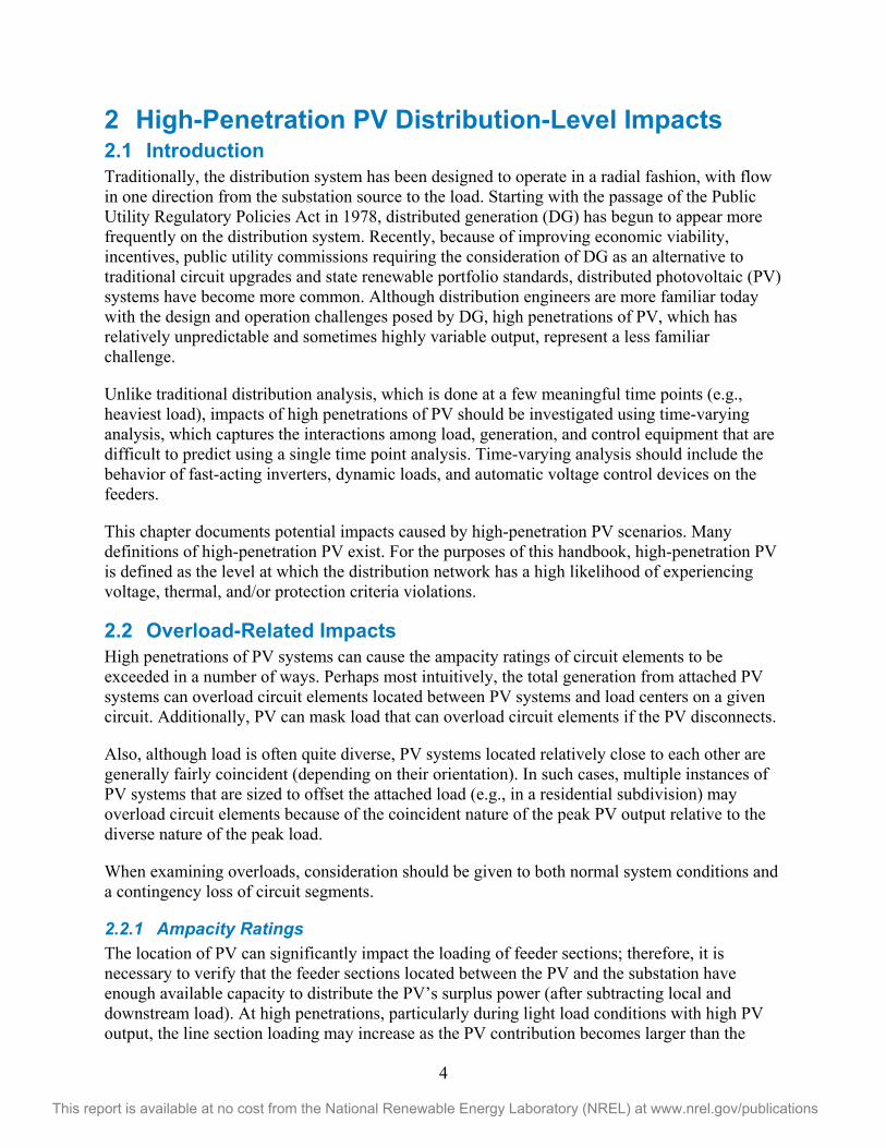
2.2.2 Masked Load Masked load refers to load that is hidden from upstream components by PV or other sources of generation. Because many forms of DG are not monitored and can be disconnected or otherwise absent without prior utility knowledge, it is important that the total load is considered in design and operation practices. For the purposes of this report, the load attached to the circuit is referred to as native load.
Figure 2.1 shows the measured load, native load, and PV generation for a peak load day. The native load (gray line) of this circuit is much higher than the measured flow (light blue line) on the circuit, because the measured circuit flow is the combination of the native load and the PV generation (dark blue line). If decisions are made based on the measurements instead of the native load calculations, significant overloads of circuit elements may occur if the PV disconnects unexpectedly. This example illustrates the issue with basing design and operation practices on measured load.
Figure 2.1. Masked load—difference between measured load and native load on a peak load day
(Mather et al. 2014)
2.2.3 Cold Load Pickup Cold load pickup takes place when a distribution circuit is reenergized after a long outage. In this situation, the loss of load diversity coupled with inrush currents can result in feeder current levels that may be much higher than the feeder’s annual peak load. This may result in overloads and low voltages if the protection system does not trip first.
PV can exacerbate the cold load pickup problem by increasing the difference between the pre-fault measured load current and the post-fault cold load pickup current. Solar PV is typically tripped when a fault occurs. If the PV cannot reconnect to the system automatically after the fault
-1000
0
1000
2000
3000
4000
5000
6000
7000
8000
0 5 10 15 20 25
Peak ckt Meas Peak ckt Load Total PV
6
This report is available at no cost from the National Renewable Energy Laboratory (NREL) at www.nrel.gov/publications
is cleared (or system operators who could do so are not on standby), or if pre-fault generation levels are no longer available, the load picked up by the substation or the feeder’s primary power source is a larger multiple of the pre-fault load compared to a scenario in which the feeder does not have solar PV.
Therefore, an assessment of the cold load pickup may be necessary when considering integrating large amounts of PV into the distribution system. Thus, again, determining the native load is of prime importance in designing circuits with high penetrations of PV.
More information about cold load pickup, as it pertains to system protection impacts, can be found in section 2.5.11.
2.3 Voltage-Related Impacts High penetrations of PV can impact circuit voltage in a number of ways. Voltage rise and voltage variations caused by fluctuations in solar PV generation are two of the most prominent and potentially problematic impacts of high penetrations of PV. These effects are particularly pronounced when large amounts of solar PV are connected near the end of long and lightly loaded feeders. Real and reactive power production from the PV system can impact the steady-state circuit voltage, and rise and fall of PV output can result in voltage fluctuations on the circuit. This, in turn, impacts power quality and voltage control device operation. Potential PV impacts on voltage are discussed below.
2.3.1 Feeder Voltage Profile With the addition of another power source internal to the distribution circuit, the voltage profile along the circuit may improve when the PV is operating.
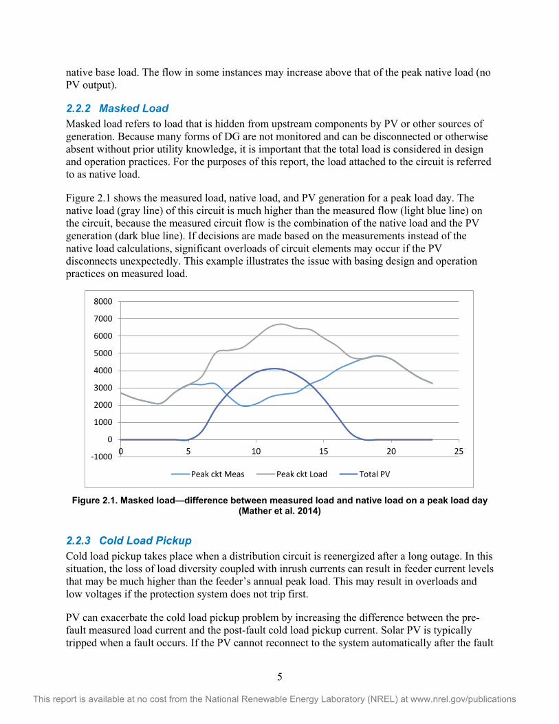
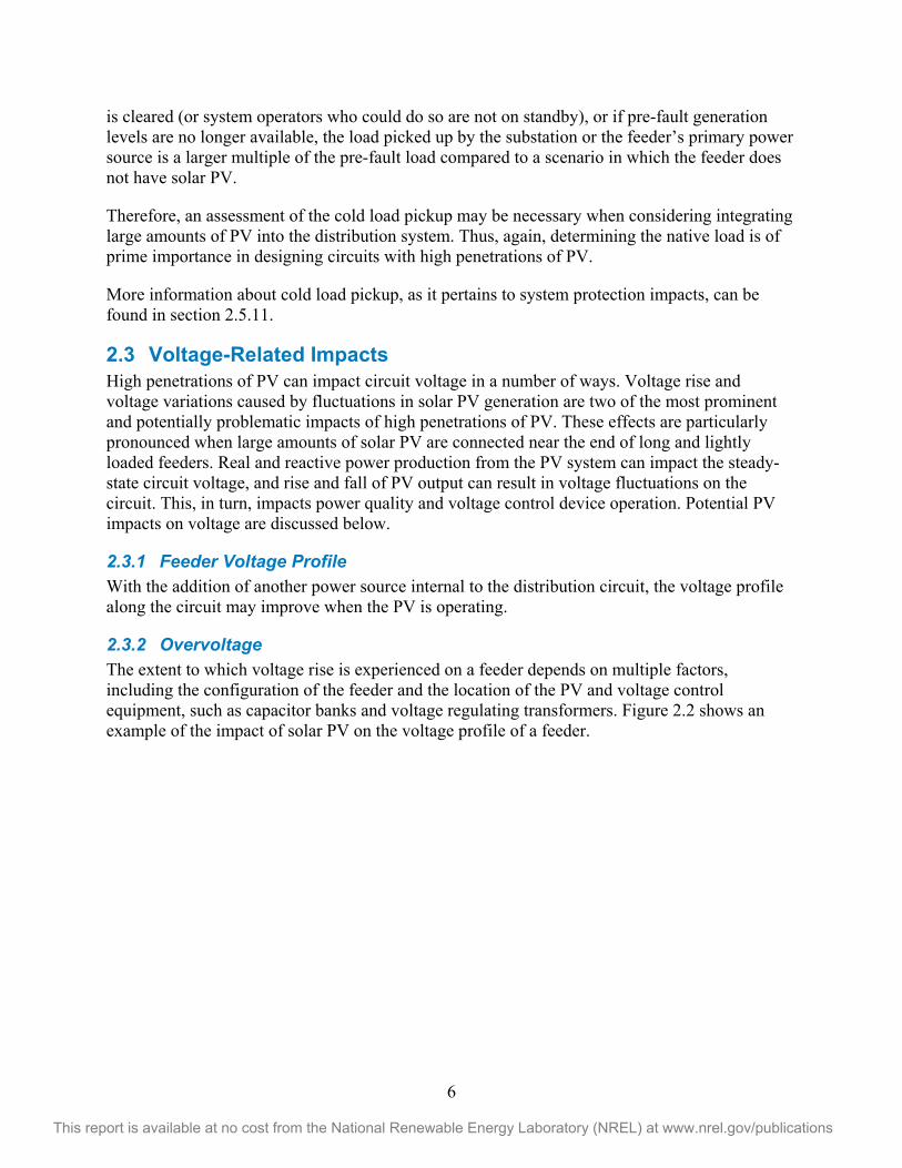
2.3.2 Overvoltage The extent to which voltage rise is experienced on a feeder depends on multiple factors, including the configuration of the feeder and the location of the PV and voltage control equipment, such as capacitor banks and voltage regulating transformers. Figure 2.2 shows an example of the impact of solar PV on the voltage profile of a feeder.
7
This report is available at no cost from the National Renewable Energy Laboratory (NREL) at www.nrel.gov/publications
Figure 2.2. Impact of solar PV on the voltage profile of a feeder
Pockets of high voltage can occur on the distribution circuit during low-load conditions, particularly in places that have a single large PV system or a cluster of PV systems. Voltages should stay below the permissible high-voltage thresholds; otherwise, they can reduce the life of electrical equipment and cause DG (including PV inverters) to trip off-line.
2.3.3 Potential for Increased Substation Voltage If a regulator or a load tap changer (LTC) transformer is not available at the substation, feeder head voltage may start to rise above acceptable limits. Even with the availability of substation regulation, studies should determine whether sufficient headroom (regulation room) exists to allow the regulator or the LTC to maintain the voltage within permissible limits over the entire load spectrum.
2.3.4 Flicker The Institute of Electrical and Electronics Engineers (IEEE) Standard 1453TM-2011 explains voltage flicker as follows:
8
This report is available at no cost from the National Renewable Energy Laboratory (NREL) at www.nrel.gov/publications
Voltage fluctuations on electric power systems sometimes give rise to noticeable illumination changes from lighting equipment. The frequency of these voltage fluctuations is much less than the 50 Hz or 60 Hz supply frequency; however, they may occur with enough frequency and magnitude to cause irritation for people observing the illumination changes.
Variations in PV output resulting from cloud cover or shading can cause fluctuations in customer service voltage. Although not common, these voltage violations can cause flicker, which may be irritating to customers and may also result in malfunctioning appliances. Maximum PV power generation on a particular feeder should be constrained to prevent unacceptable flicker; this could set an upper limit on the total connected PV capacity on that feeder. Solar PV impact studies should be performed to assess the potential of voltage flicker due to high penetrations of solar PV.
2.3.5 Automatic Voltage Regulation Equipment Voltage regulation practices used in radial power distribution systems have traditionally been designed with the assumption that the substation is the only power source in the system (McGranaghan et al. 2008), which implies that all flow is outward from the substation toward the end of the feeder. Voltage on such feeders is typically regulated by the LTC at the substation, voltage regulators at the start of the feeders and sometimes distributed throughout the feeders, and switched capacitor banks distributed throughout the feeders. The control settings of these devices are coordinated to maintain the desired voltage profile along the feeder (McGranaghan et al. 2008).
After PV is added to the distribution system, the assumption that the substation is the only power source no longer holds true, and the problems of voltage rise/fall and flicker associated with solar PV as discussed earlier can lead to frequent operation of LTCs, voltage regulators, and switched capacitor banks, resulting in additional step-voltage changes. Further, more frequent operation of these devices may shorten their life cycles and increase maintenance requirements (Katiraei and Agüero 2011).
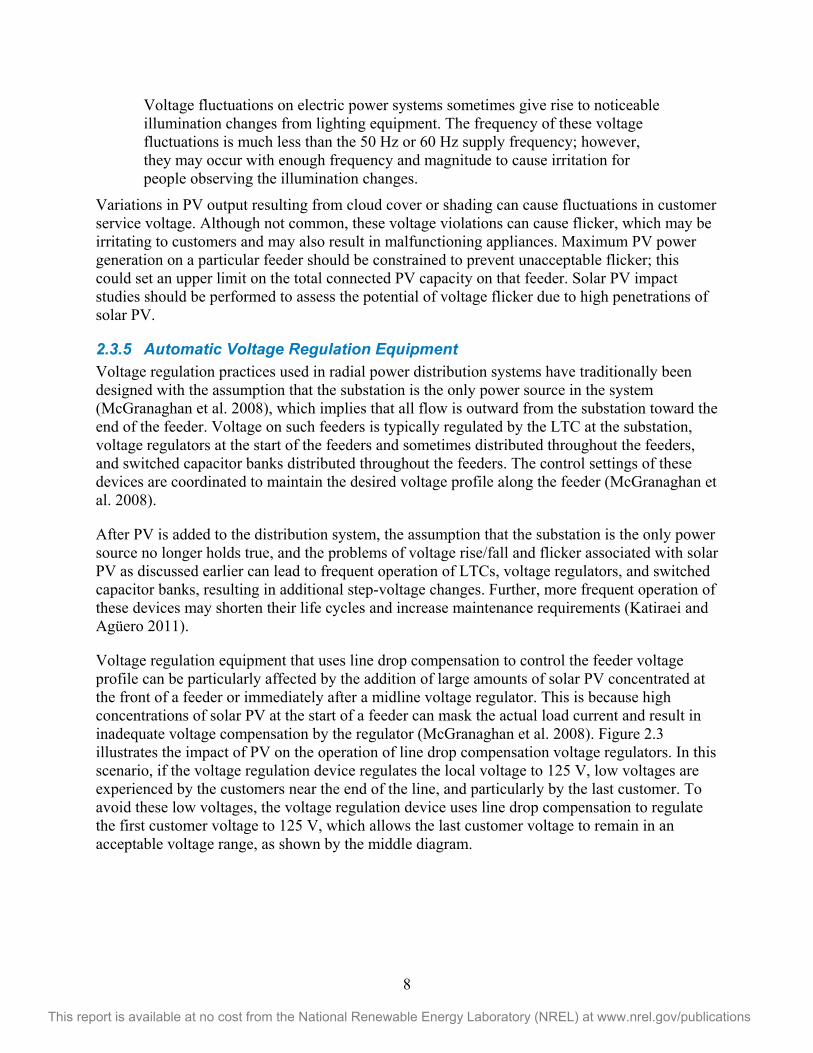
Voltage regulation equipment that uses line drop compensation to control the feeder voltage profile can be particularly affected by the addition of large amounts of solar PV concentrated at the front of a feeder or immediately after a midline voltage regulator. This is because high concentrations of solar PV at the start of a feeder can mask the actual load current and result in inadequate voltage compensation by the regulator (McGranaghan et al. 2008). Figure 2.3 illustrates the impact of PV on the operation of line drop compensation voltage regulators. In this scenario, if the voltage regulation device regulates the local voltage to 125 V, low voltages are experienced by the customers near the end of the line, and particularly by the last customer. To avoid these low voltages, the voltage regulation device uses line drop compensation to regulate the first customer voltage to 125 V, which allows the last customer voltage to remain in an acceptable voltage range, as shown by the middle diagram.
9
This report is available at no cost from the National Renewable Energy Laboratory (NREL) at www.nrel.gov/publications
Figure 2.3. Impact of solar PV on voltage compensation provided by line drop compensation.
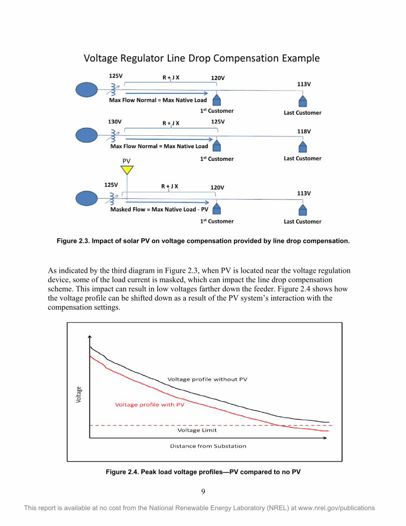
As indicated by the third diagram in Figure 2.3, when PV is located near the voltage regulation device, some of the load current is masked, which can impact the line drop compensation scheme. This impact can result in low voltages farther down the feeder. Figure 2.4 shows how the voltage profile can be shifted down as a result of the PV system’s interaction with the compensation settings.
Figure 2.4. Peak load voltage profiles—PV compared to no PV
10
This report is available at no cost from the National Renewable Energy Laboratory (NREL) at www.nrel.gov/publications
2.4 Reverse Power Flow Impacts Reverse power flow on a distribution system upstream of a PV system may occur during times of light load and high PV generation. Reverse flow can cause problems for the protection system, as previously noted, and for the voltage regulators. Voltage regulators may be unidirectional and not designed to accommodate reverse flow (see Section 2.4.3). If voltage regulators are bidirectional, modifications to the regulator control may still be necessary to accommodate the reverse flow.
2.4.1 Substation and Bulk System Impacts Impacts depend on factors such as penetration level, aggregated output characteristics, and system characteristics (e.g., amount and type of other generation sources). Most common concerns include increases in cost because of regulation, ramping generation, scheduling generation, and unit commitment, which may degrade balancing authority area performance and wear and tear on regulating units.
2.4.1.1 Reverse Power Flow to Adjacent Circuits Protection concerns, arising from significant reverse power flows, such as exceeding interruption ratings of circuit protection elements and sympathetic tripping of adjacent circuits are two of many ways in which distribution-connected PV or other forms of DG-caused fault current contributions lead to problems on the distribution system.
2.4.1.2 Reverse Power Flow Through the Substation Transformer Reverse power flows resulting from PV generation could possibly cause reverse power relays at a substation to operate, disconnecting the associated circuit. The resulting outages ultimately reduce system reliability.
2.4.2 Temporary and Transient Overvoltage IEEE C62.82.1-2010 defines temporary overvoltage (TOV) as follows:
An oscillatory phase-to-ground or phase-to-phase overvoltage that is at a given location of relatively long duration (seconds, even minutes) and that is undamped or only weakly damped. Temporary overvoltages usually originate from switching operations or faults (e.g., load rejection, single-phase fault, fault on a high-resistance grounded or ungrounded system) or from nonlinearities (e.g., ferroresonance effects, harmonics), or both. They are characterized by the amplitude, the oscillation frequencies, the total duration, or the decrement.
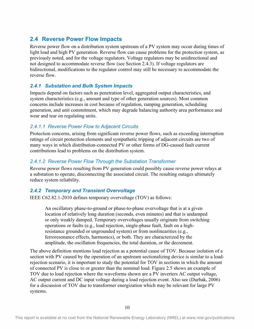
The above definition mentions load rejection as a potential cause of TOV. Because isolation of a section with PV caused by the operation of an upstream sectionalizing device is similar to a load-rejection scenario, it is important to study the potential for TOV in sections in which the amount of connected PV is close to or greater than the nominal load. Figure 2.5 shows an example of TOV due to load rejection where the waveforms shown are a PV inverters AC output voltage, AC output current and DC input voltage during a load rejection event. Also see (Durbak, 2006) for a discussion of TOV due to transformer energization which may be relevant for large PV systems.
11
This report is available at no cost from the National Renewable Energy Laboratory (NREL) at www.nrel.gov/publications
Figure 2.5. Example of TOV due to load rejection (Nelson et al. 2015)
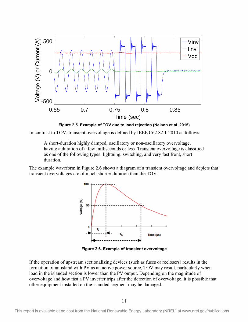
In contrast to TOV, transient overvoltage is defined by IEEE C62.82.1-2010 as follows:
A short-duration highly damped, oscillatory or non-oscillatory overvoltage, having a duration of a few milliseconds or less. Transient overvoltage is classified as one of the following types: lightning, switching, and very fast front, short duration.
The example waveform in Figure 2.6 shows a diagram of a transient overvoltage and depicts that transient overvoltages are of much shorter duration than the TOV.
Figure 2.6. Example of transient overvoltage
If the operation of upstream sectionalizing devices (such as fuses or reclosers) results in the formation of an island with PV as an active power source, TOV may result, particularly when load in the islanded section is lower than the PV output. Depending on the magnitude of overvoltage and how fast a PV inverter trips after the detection of overvoltage, it is possible that other equipment installed on the islanded segment may be damaged.
12
This report is available at no cost from the National Renewable Energy Laboratory (NREL) at www.nrel.gov/publications
The operation of a protective device or other switchable device that isolates an amount of load with an aggregate amount of PV in excess of the load may result in an overvoltage condition. Studies that show reverse flow through a protective device should alert the planning engineer to this possibility, because there is more generation than load on the section beyond the protective device.
A steady-state network analysis that assumes an unchanged current output from the PV into an unchanged amount of isolated load can provide a conservative estimate of the possible overvoltage. For example, if a fixed current associated with a PV output of 1.1 MW is isolated with 1 MW of load at a power factor of 1, this approach will calculate an approximate 10% overvoltage.
Parameters needed for a detailed transient overvoltage analysis are often not known or are difficult to obtain. A standardized methodology for performing such a study is beyond the scope of this handbook.
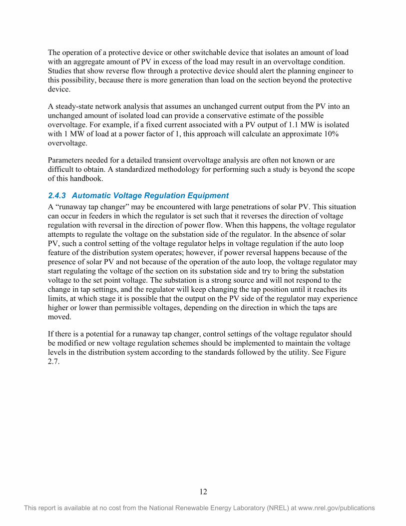
2.4.3 Automatic Voltage Regulation Equipment A “runaway tap changer” may be encountered with large penetrations of solar PV. This situation can occur in feeders in which the regulator is set such that it reverses the direction of voltage regulation with reversal in the direction of power flow. When this happens, the voltage regulator attempts to regulate the voltage on the substation side of the regulator. In the absence of solar PV, such a control setting of the voltage regulator helps in voltage regulation if the auto loop feature of the distribution system operates; however, if power reversal happens because of the presence of solar PV and not because of the operation of the auto loop, the voltage regulator may start regulating the voltage of the section on its substation side and try to bring the substation voltage to the set point voltage. The substation is a strong source and will not respond to the change in tap settings, and the regulator will keep changing the tap position until it reaches its limits, at which stage it is possible that the output on the PV side of the regulator may experience higher or lower than permissible voltages, depending on the direction in which the taps are moved.
If there is a potential for a runaway tap changer, control settings of the voltage regulator should be modified or new voltage regulation schemes should be implemented to maintain the voltage levels in the distribution system according to the standards followed by the utility. See Figure 2.7.
13
This report is available at no cost from the National Renewable Energy Laboratory (NREL) at www.nrel.gov/publications
Figure 2.7. Runaway voltage regulator
2.5 System Protection Impacts High penetrations of PV can change the fault current levels and also make it necessary to review the protection coordination currently implemented in the distribution network. In this section, the key impacts of high penetrations of PV on the distribution system protection are discussed.
2.5.1 Fault Current and Interrupting Rating The addition of PV increases the fault current levels at all points on the system; therefore, it is important to verify that the maximum fault current through each protective device does not exceed its interrupting rating. Typically, utilities require the interrupting rating to exceed the maximum fault current by a safety margin of approximately 10%, but any applicable margins for this area should be considered. In addition, direct-current offsets that occur when the X/R ratio of the Thevenin impedance is high should also be considered. Some manufacturers specify their interrupting ratings at an X/R ratio of 15 or less. Equipment interruption ratings in most cases are given for the symmetrical fault level and list the maximum X/R ratio.
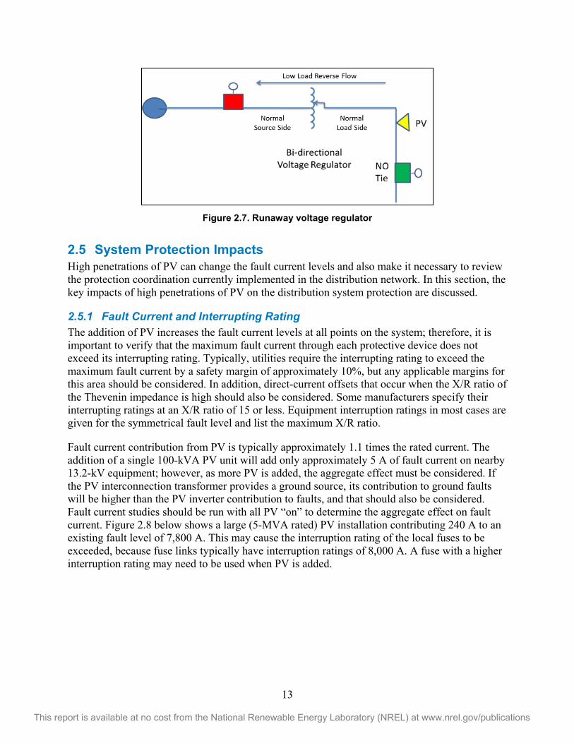
Fault current contribution from PV is typically approximately 1.1 times the rated current. The addition of a single 100-kVA PV unit will add only approximately 5 A of fault current on nearby 13.2-kV equipment; however, as more PV is added, the aggregate effect must be considered. If the PV interconnection transformer provides a ground source, its contribution to ground faults will be higher than the PV inverter contribution to faults, and that should also be considered. Fault current studies should be run with all PV “on” to determine the aggregate effect on fault current. Figure 2.8 below shows a large (5-MVA rated) PV installation contributing 240 A to an existing fault level of 7,800 A. This may cause the interruption rating of the local fuses to be exceeded, because fuse links typically have interruption ratings of 8,000 A. A fuse with a higher interruption rating may need to be used when PV is added.
14
This report is available at no cost from the National Renewable Energy Laboratory (NREL) at www.nrel.gov/publications
Figure 2.8. Impact of PV on fuse interruption ratings
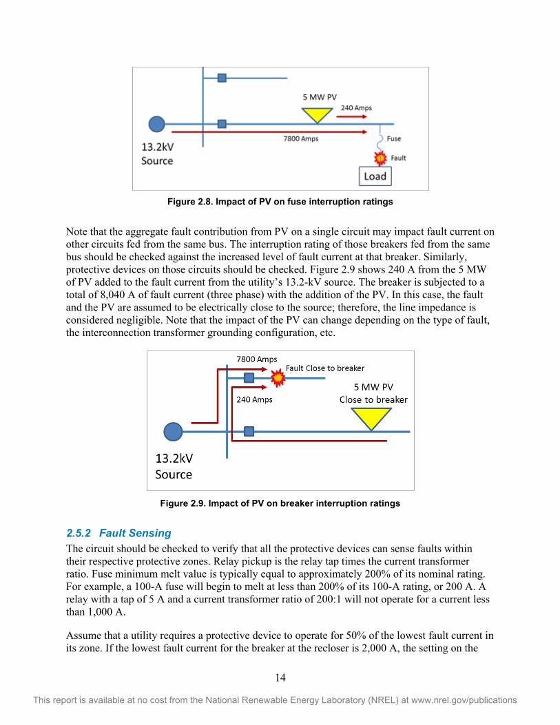
Note that the aggregate fault contribution from PV on a single circuit may impact fault current on other circuits fed from the same bus. The interruption rating of those breakers fed from the same bus should be checked against the increased level of fault current at that breaker. Similarly, protective devices on those circuits should be checked. Figure 2.9 shows 240 A from the 5 MW of PV added to the fault current from the utility’s 13.2-kV source. The breaker is subjected to a total of 8,040 A of fault current (three phase) with the addition of the PV. In this case, the fault and the PV are assumed to be electrically close to the source; therefore, the line impedance is considered negligible. Note that the impact of the PV can change depending on the type of fault, the interconnection transformer grounding configuration, etc.
Figure 2.9. Impact of PV on breaker interruption ratings
2.5.2 Fault Sensing The circuit should be checked to verify that all the protective devices can sense faults within their respective protective zones. Relay pickup is the relay tap times the current transformer ratio. Fuse minimum melt value is typically equal to approximately 200% of its nominal rating. For example, a 100-A fuse will begin to melt at less than 200% of its 100-A rating, or 200 A. A relay with a tap of 5 A and a current transformer ratio of 200:1 will not operate for a current less than 1,000 A.
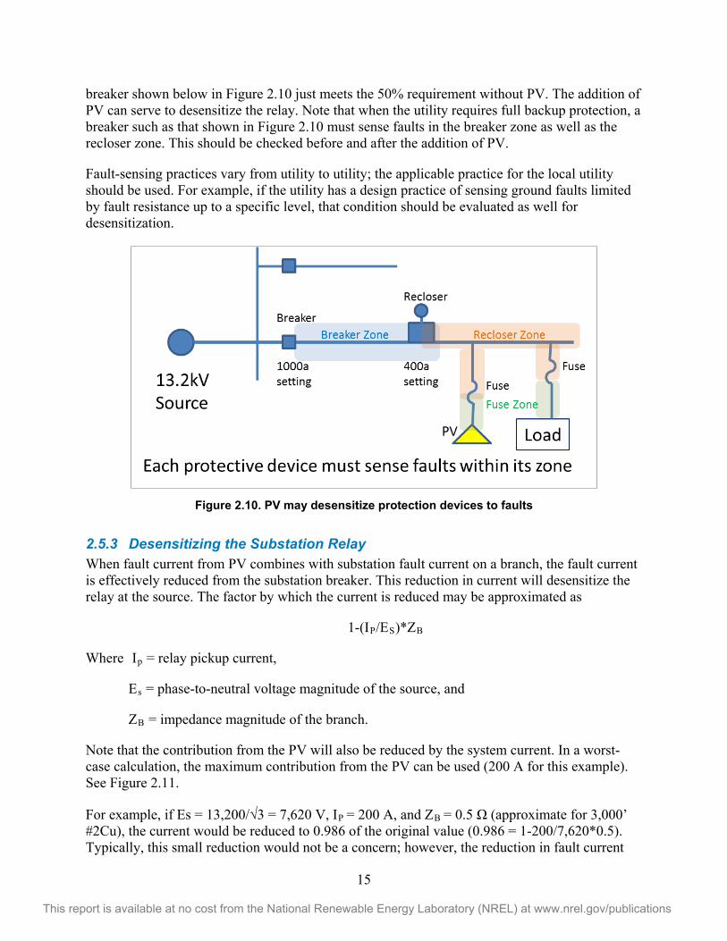
Assume that a utility requires a protective device to operate for 50% of the lowest fault current in its zone. If the lowest fault current for the breaker at the recloser is 2,000 A, the setting on the
15
This report is available at no cost from the National Renewable Energy Laboratory (NREL) at www.nrel.gov/publications
breaker shown below in Figure 2.10 just meets the 50% requirement without PV. The addition of PV can serve to desensitize the relay. Note that when the utility requires full backup protection, a breaker such as that shown in Figure 2.10 must sense faults in the breaker zone as well as the recloser zone. This should be checked before and after the addition of PV.
Fault-sensing practices vary from utility to utility; the applicable practice for the local utility should be used. For example, if the utility has a design practice of sensing ground faults limited by fault resistance up to a specific level, that condition should be evaluated as well for desensitization.
Figure 2.10. PV may desensitize protection devices to faults
2.5.3 Desensitizing the Substation Relay When fault current from PV combines with substation fault current on a branch, the fault current is effectively reduced from the substation breaker. This reduction in current will desensitize the relay at the source. The factor by which the current is reduced may be approximated as
1-(IP/ES)*ZB
Where Ip = relay pickup current,
Es = phase-to-neutral voltage magnitude of the source, and
ZB = impedance magnitude of the branch.
Note that the contribution from the PV will also be reduced by the system current. In a worst-case calculation, the maximum contribution from the PV can be used (200 A for this example). See Figure 2.11.
For example, if Es = 13,200/ 3 = 7,620 V, IP = 200 A, and ZB = 0.5 (approximate for 3,000’ #2Cu), the current would be reduced to 0.986 of the original value (0.986 = 1-200/7,620*0.5). Typically, this small reduction would not be a concern; however, the reduction in fault current
16
This report is available at no cost from the National Renewable Energy Laboratory (NREL) at www.nrel.gov/publications
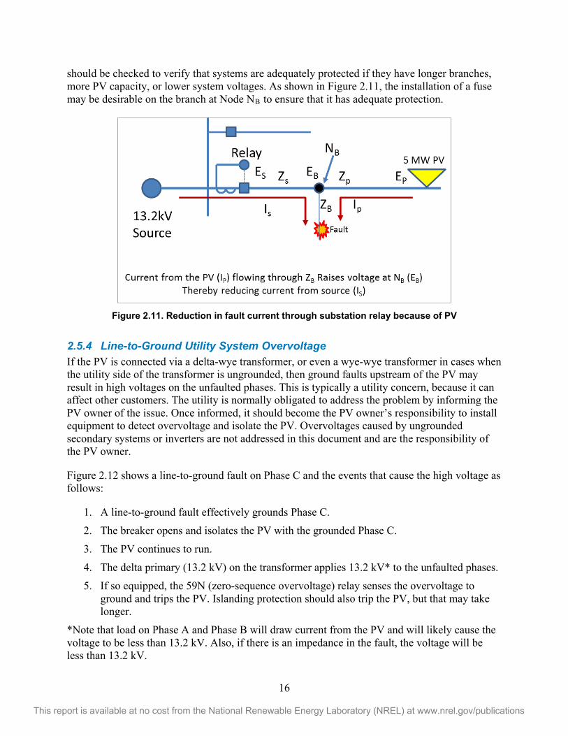
should be checked to verify that systems are adequately protected if they have longer branches, more PV capacity, or lower system voltages. As shown in Figure 2.11, the installation of a fuse may be desirable on the branch at Node NB to ensure that it has adequate protection.
Figure 2.11. Reduction in fault current through substation relay because of PV
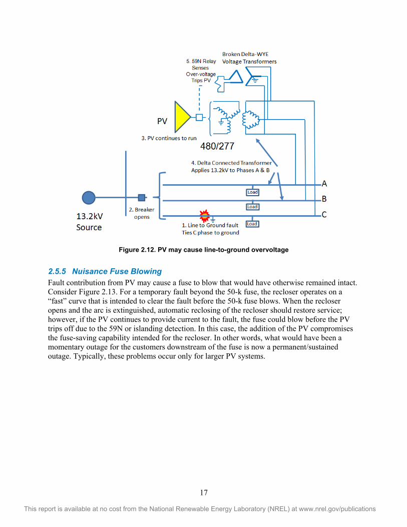
2.5.4 Line-to-Ground Utility System Overvoltage If the PV is connected via a delta-wye transformer, or even a wye-wye transformer in cases when the utility side of the transformer is ungrounded, then ground faults upstream of the PV may result in high voltages on the unfaulted phases. This is typically a utility concern, because it can affect other customers. The utility is normally obligated to address the problem by informing the PV owner of the issue. Once informed, it should become the PV owner’s responsibility to install equipment to detect overvoltage and isolate the PV. Overvoltages caused by ungrounded secondary systems or inverters are not addressed in this document and are the responsibility of the PV owner.
Figure 2.12 shows a line-to-ground fault on Phase C and the events that cause the high voltage as follows:
1. A line-to-ground fault effectively grounds Phase C.
2. The breaker opens and isolates the PV with the grounded Phase C.
3. The PV continues to run.
4. The delta primary (13.2 kV) on the transformer applies 13.2 kV* to the unfaulted phases.
5. If so equipped, the 59N (zero-sequence overvoltage) relay senses the overvoltage to ground and trips the PV. Islanding protection should also trip the PV, but that may take longer.
*Note that load on Phase A and Phase B will draw current from the PV and will likely cause the voltage to be less than 13.2 kV. Also, if there is an impedance in the fault, the voltage will be less than 13.2 kV.
17
This report is available at no cost from the National Renewable Energy Laboratory (NREL) at www.nrel.gov/publications
Figure 2.12. PV may cause line-to-ground overvoltage
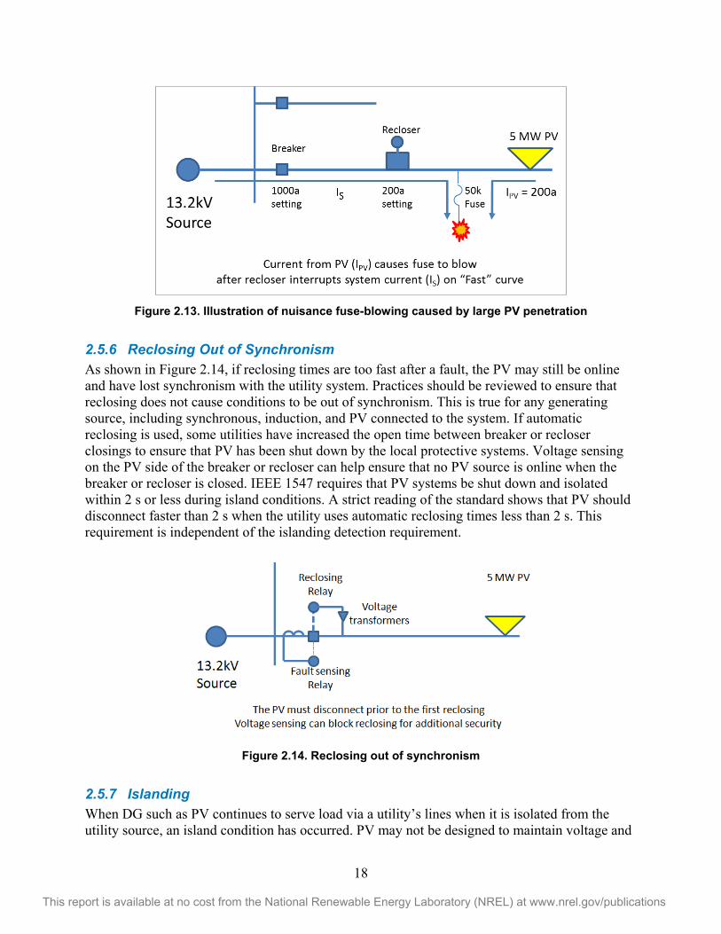
2.5.5 Nuisance Fuse Blowing Fault contribution from PV may cause a fuse to blow that would have otherwise remained intact. Consider Figure 2.13. For a temporary fault beyond the 50-k fuse, the recloser operates on a “fast” curve that is intended to clear the fault before the 50-k fuse blows. When the recloser opens and the arc is extinguished, automatic reclosing of the recloser should restore service; however, if the PV continues to provide current to the fault, the fuse could blow before the PV trips off due to the 59N or islanding detection. In this case, the addition of the PV compromises the fuse-saving capability intended for the recloser. In other words, what would have been a momentary outage for the customers downstream of the fuse is now a permanent/sustained outage. Typically, these problems occur only for larger PV systems.
18
This report is available at no cost from the National Renewable Energy Laboratory (NREL) at www.nrel.gov/publications
Figure 2.13. Illustration of nuisance fuse-blowing caused by large PV penetration
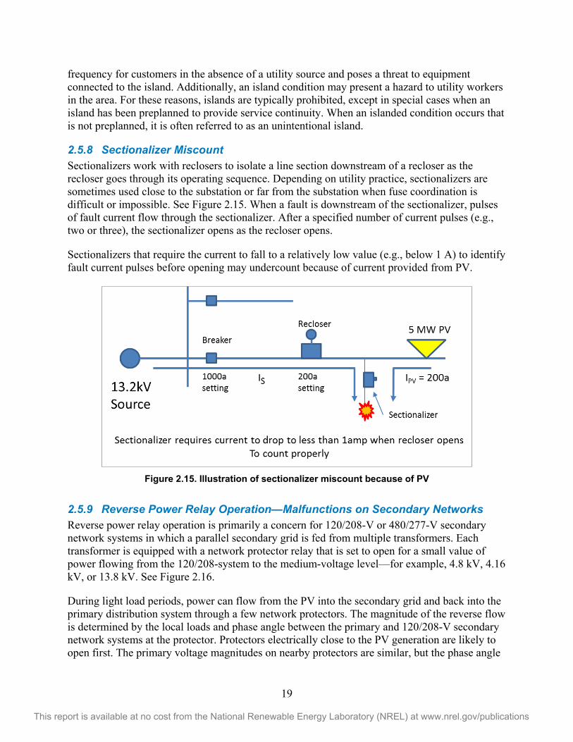
2.5.6 Reclosing Out of Synchronism As shown in Figure 2.14, if reclosing times are too fast after a fault, the PV may still be online and have lost synchronism with the utility system. Practices should be reviewed to ensure that reclosing does not cause conditions to be out of synchronism. This is true for any generating source, including synchronous, induction, and PV connected to the system. If automatic reclosing is used, some utilities have increased the open time between breaker or recloser closings to ensure that PV has been shut down by the local protective systems. Voltage sensing on the PV side of the breaker or recloser can help ensure that no PV source is online when the breaker or recloser is closed. IEEE 1547 requires that PV systems be shut down and isolated within 2 s or less during island conditions. A strict reading of the standard shows that PV should disconnect faster than 2 s when the utility uses automatic reclosing times less than 2 s. This requirement is independent of the islanding detection requirement.
Figure 2.14. Reclosing out of synchronism
2.5.7 Islanding When DG such as PV continues to serve load via a utility’s lines when it is isolated from the utility source, an island condition has occurred. PV may not be designed to maintain voltage and
19
This report is available at no cost from the National Renewable Energy Laboratory (NREL) at www.nrel.gov/publications
frequency for customers in the absence of a utility source and poses a threat to equipment connected to the island. Additionally, an island condition may present a hazard to utility workers in the area. For these reasons, islands are typically prohibited, except in special cases when an island has been preplanned to provide service continuity. When an islanded condition occurs that is not preplanned, it is often referred to as an unintentional island.
2.5.8 Sectionalizer Miscount Sectionalizers work with reclosers to isolate a line section downstream of a recloser as the recloser goes through its operating sequence. Depending on utility practice, sectionalizers are sometimes used close to the substation or far from the substation when fuse coordination is difficult or impossible. See Figure 2.15. When a fault is downstream of the sectionalizer, pulses of fault current flow through the sectionalizer. After a specified number of current pulses (e.g., two or three), the sectionalizer opens as the recloser opens.
Sectionalizers that require the current to fall to a relatively low value (e.g., below 1 A) to identify fault current pulses before opening may undercount because of current provided from PV.
Figure 2.15. Illustration of sectionalizer miscount because of PV
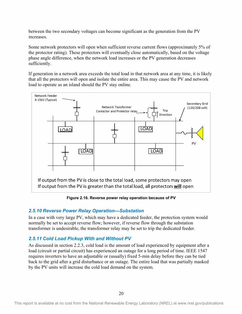
2.5.9 Reverse Power Relay Operation—Malfunctions on Secondary Networks Reverse power relay operation is primarily a concern for 120/208-V or 480/277-V secondary network systems in which a parallel secondary grid is fed from multiple transformers. Each transformer is equipped with a network protector relay that is set to open for a small value of power flowing from the 120/208-system to the medium-voltage level—for example, 4.8 kV, 4.16 kV, or 13.8 kV. See Figure 2.16.
During light load periods, power can flow from the PV into the secondary grid and back into the primary distribution system through a few network protectors. The magnitude of the reverse flow is determined by the local loads and phase angle between the primary and 120/208-V secondary network systems at the protector. Protectors electrically close to the PV generation are likely to open first. The primary voltage magnitudes on nearby protectors are similar, but the phase angle
20
This report is available at no cost from the National Renewable Energy Laboratory (NREL) at www.nrel.gov/publications
between the two secondary voltages can become significant as the generation from the PV increases.
Some network protectors will open when sufficient reverse current flows (approximately 5% of the protector rating). These protectors will eventually close automatically, based on the voltage phase angle difference, when the network load increases or the PV generation decreases sufficiently.
If generation in a network area exceeds the total load in that network area at any time, it is likely that all the protectors will open and isolate the entire area. This may cause the PV and network load to operate as an island should the PV stay online.
Figure 2.16. Reverse power relay operation because of PV
2.5.10 Reverse Power Relay Operation—Substation In a case with very large PV, which may have a dedicated feeder, the protection system would normally be set to accept reverse flow; however, if reverse flow through the substation transformer is undesirable, the transformer relay may be set to trip the dedicated feeder.
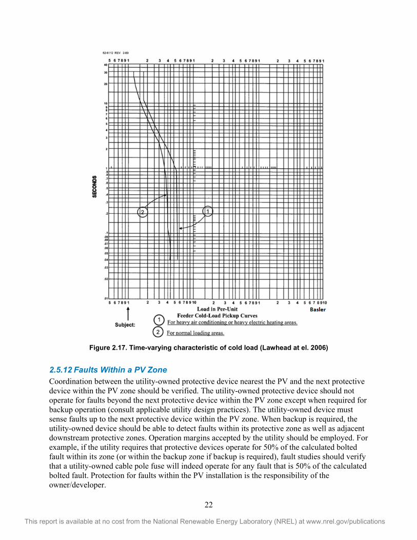
2.5.11 Cold Load Pickup With and Without PV As discussed in section 2.2.3, cold load is the amount of load experienced by equipment after a load (circuit or partial circuit) has experienced an outage for a long period of time. IEEE 1547 requires inverters to have an adjustable or (usually) fixed 5-min delay before they can be tied back to the grid after a grid disturbance or an outage. The entire load that was partially masked by the PV units will increase the cold load demand on the system.

21
This report is available at no cost from the National Renewable Energy Laboratory (NREL) at www.nrel.gov/publications
The cold load demand on the system is typically highest during the first few minutes after the power comes back on following an extended outage. Motors may all start simultaneously. In the winter, the heating load to be picked up may be very large because of loss of diversity. The cold load demand will depend upon the duration of the outage. Various tables and curves are available showing the expected increase in initial cold load to be picked up in multiples of pre-outage load. This information is available for different classes of loads and provides the characteristic of the time-varying load restored after an extended outage. Output from PV will affect the amount of normal load actually measured or calculated. Figure 2.17 shows a sample of the time-varying characteristic of cold load.
Note that the data are typically based on pre-outage normal load. The effect of PV may mask what the normal load actually is at the start-of-circuit or any monitoring point. This effect should be taken into account when determining the load to be picked up. Also, during daylight hours any automatic return of PV to the system may impact and actually mitigate the effect of cold load pickup. Equipment and protective devices should be rated for the increased amount of expected cold load without considering potential cold load pickup mitigation from PV as the availability of PV to mitigate cold load pickup is not certain. Whenever possible, protective devices should be sized to not operate for this increased amount of load.
22
This report is available at no cost from the National Renewable Energy Laboratory (NREL) at www.nrel.gov/publications
Figure 2.17. Time-varying characteristic of cold load (Lawhead at el. 2006)
2.5.12 Faults Within a PV Zone Coordination between the utility-owned protective device nearest the PV and the next protective device within the PV zone should be verified. The utility-owned protective device should not operate for faults beyond the next protective device within the PV zone except when required for backup operation (consult applicable utility design practices). The utility-owned device must sense faults up to the next protective device within the PV zone. When backup is required, the utility-owned device should be able to detect faults within its protective zone as well as adjacent downstream protective zones. Operation margins accepted by the utility should be employed. For example, if the utility requires that protective devices operate for 50% of the calculated bolted fault within its zone (or within the backup zone if backup is required), fault studies should verify that a utility-owned cable pole fuse will indeed operate for any fault that is 50% of the calculated bolted fault. Protection for faults within the PV installation is the responsibility of the owner/developer.
23
This report is available at no cost from the National Renewable Energy Laboratory (NREL) at www.nrel.gov/publications
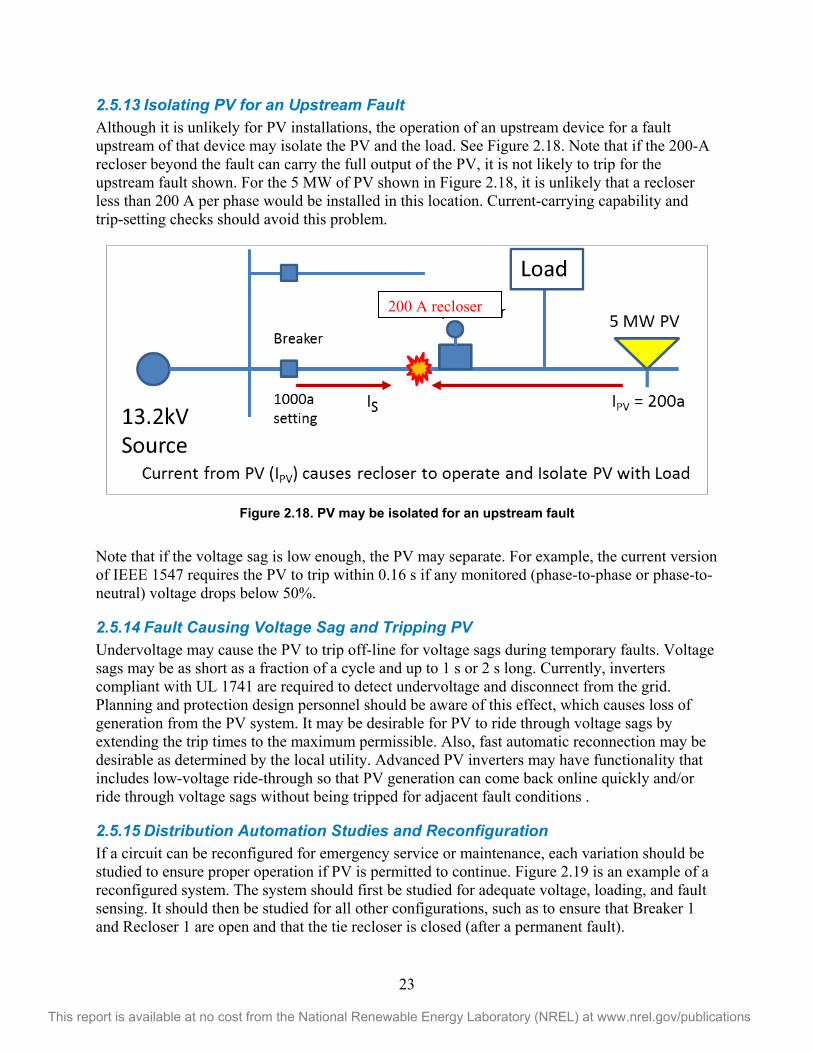
2.5.13 Isolating PV for an Upstream Fault Although it is unlikely for PV installations, the operation of an upstream device for a fault upstream of that device may isolate the PV and the load. See Figure 2.18. Note that if the 200-A recloser beyond the fault can carry the full output of the PV, it is not likely to trip for the upstream fault shown. For the 5 MW of PV shown in Figure 2.18, it is unlikely that a recloser less than 200 A per phase would be installed in this location. Current-carrying capability and trip-setting checks should avoid this problem.
Figure 2.18. PV may be isolated for an upstream fault
Note that if the voltage sag is low enough, the PV may separate. For example, the current version of IEEE 1547 requires the PV to trip within 0.16 s if any monitored (phase-to-phase or phase-to-neutral) voltage drops below 50%.
2.5.14 Fault Causing Voltage Sag and Tripping PV Undervoltage may cause the PV to trip off-line for voltage sags during temporary faults. Voltage sags may be as short as a fraction of a cycle and up to 1 s or 2 s long. Currently, inverters compliant with UL 1741 are required to detect undervoltage and disconnect from the grid. Planning and protection design personnel should be aware of this effect, which causes loss of generation from the PV system. It may be desirable for PV to ride through voltage sags by extending the trip times to the maximum permissible. Also, fast automatic reconnection may be desirable as determined by the local utility. Advanced PV inverters may have functionality that includes low-voltage ride-through so that PV generation can come back online quickly and/or ride through voltage sags without being tripped for adjacent fault conditions .
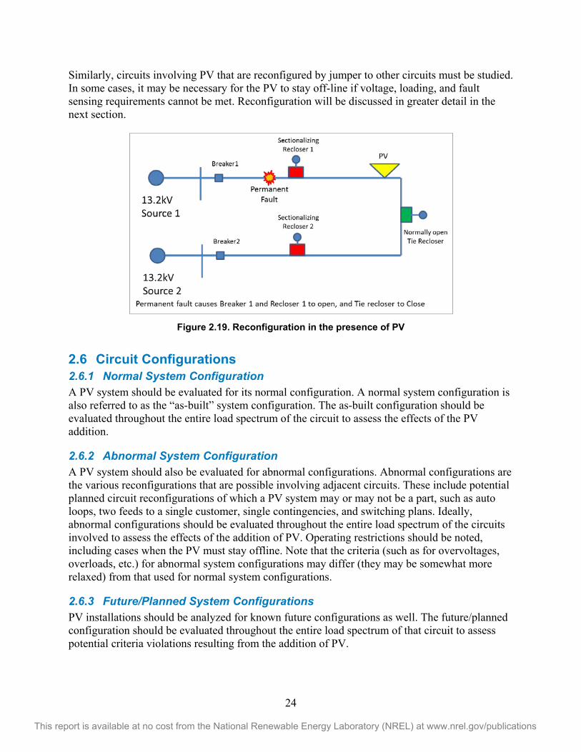
2.5.15 Distribution Automation Studies and Reconfiguration If a circuit can be reconfigured for emergency service or maintenance, each variation should be studied to ensure proper operation if PV is permitted to continue. Figure 2.19 is an example of a reconfigured system. The system should first be studied for adequate voltage, loading, and fault sensing. It should then be studied for all other configurations, such as to ensure that Breaker 1 and Recloser 1 are open and that the tie recloser is closed (after a permanent fault).
200 A recloser
24
This report is available at no cost from the National Renewable Energy Laboratory (NREL) at www.nrel.gov/publications
Similarly, circuits involving PV that are reconfigured by jumper to other circuits must be studied. In some cases, it may be necessary for the PV to stay off-line if voltage, loading, and fault sensing requirements cannot be met. Reconfiguration will be discussed in greater detail in the next section.
Figure 2.19. Reconfiguration in the presence of PV
2.6 Circuit Configurations 2.6.1 Normal System Configuration A PV system should be evaluated for its normal configuration. A normal system configuration is also referred to as the “as-built” system configuration. The as-built configuration should be evaluated throughout the entire load spectrum of the circuit to assess the effects of the PV addition.
2.6.2 Abnormal System Configuration A PV system should also be evaluated for abnormal configurations. Abnormal configurations are the various reconfigurations that are possible involving adjacent circuits. These include potential planned circuit reconfigurations of which a PV system may or may not be a part, such as auto loops, two feeds to a single customer, single contingencies, and switching plans. Ideally, abnormal configurations should be evaluated throughout the entire load spectrum of the circuits involved to assess the effects of the addition of PV. Operating restrictions should be noted, including cases when the PV must stay offline. Note that the criteria (such as for overvoltages, overloads, etc.) for abnormal system configurations may differ (they may be somewhat more relaxed) from that used for normal system configurations.
2.6.3 Future/Planned System Configurations PV installations should be analyzed for known future configurations as well. The future/planned configuration should be evaluated throughout the entire load spectrum of that circuit to assess potential criteria violations resulting from the addition of PV.
25
This report is available at no cost from the National Renewable Energy Laboratory (NREL) at www.nrel.gov/publications
2.6.4 Contingency Conditions Contingency conditions refer to abnormal system conditions that may arise because of events such as loss of load, tripping of a line, or failure of protective devices.
The need to analyze the impact of PV during normal and abnormal circuit configurations and also during contingency conditions is illustrated with two examples.
2.6.4.1 Example 1 An example of an auto loop system configuration is shown in Figure 2.20. Figure 2.20 (a) shows an auto loop circuit in its normal configuration; Figure 2.20 (b) shows the same auto loop in an abnormal configuration in which a fault has been isolated and the tie reclosed to automatically pick up a portion of the circuit that had experienced an outage. Because all PV is disconnected during a feeder outage, when the tie recloser is closed, the feeder-loading capability could be exceeded. This is particularly a problem if the decision to close the tie recloser was made based on the flow through the isolating line recloser. Thus, as demonstrated before, it is important to determine the actual native load when reviewing the potential impact on switching plans, both with and without PV.
Figure 2.20. (a) Normal and (b) abnormal configuration of an auto loop system, red indicates a
closed switch, green indicates an open switch
2.6.4.2 Example 2 Figure 2.21 shows three scenarios: an example for peak load, light load, and contingency loading. In the peak load example (top), no overloads are noted; however, in the light load example (middle), an overload could occur on the smallest conductor. (An example of #6 Cu with a normal rating of 138 A is given.) In the contingency example (bottom), which has a loss of downstream load, an emergency overload would exist. (An example of #6 Cu with an emergency rating of 185 A is given.)
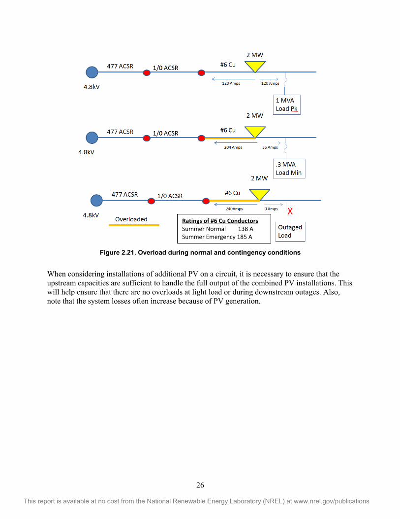
26
This report is available at no cost from the National Renewable Energy Laboratory (NREL) at www.nrel.gov/publications
Figure 2.21. Overload during normal and contingency conditions
When considering installations of additional PV on a circuit, it is necessary to ensure that the upstream capacities are sufficient to handle the full output of the combined PV installations. This will help ensure that there are no overloads at light load or during downstream outages. Also, note that the system losses often increase because of PV generation.
Ratings of #6 Cu Conductors Summer Normal 138 A Summer Emergency 185 A
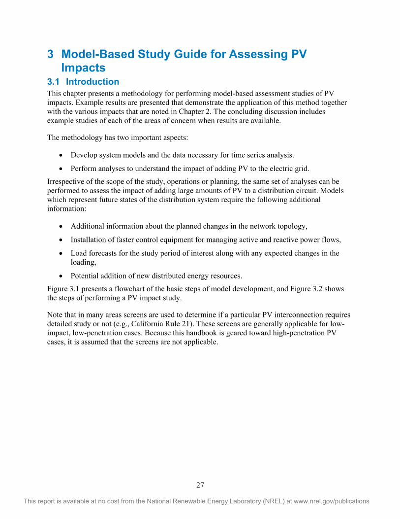
27
This report is available at no cost from the National Renewable Energy Laboratory (NREL) at www.nrel.gov/publications
3 Model-Based Study Guide for Assessing PV Impacts
3.1 Introduction This chapter presents a methodology for performing model-based assessment studies of PV impacts. Example results are presented that demonstrate the application of this method together with the various impacts that are noted in Chapter 2. The concluding discussion includes example studies of each of the areas of concern when results are available.
The methodology has two important aspects:
Develop system models and the data necessary for time series analysis.
Perform analyses to understand the impact of adding PV to the electric grid.
Irrespective of the scope of the study, operations or planning, the same set of analyses can be performed to assess the impact of adding large amounts of PV to a distribution circuit. Models which represent future states of the distribution system require the following additional information:
Additional information about the planned changes in the network topology,
Installation of faster control equipment for managing active and reactive power flows,
Load forecasts for the study period of interest along with any expected changes in the loading,
Potential addition of new distributed energy resources.
Figure 3.1 presents a flowchart of the basic steps of model development, and Figure 3.2 shows the steps of performing a PV impact study.
Note that in many areas screens are used to determine if a particular PV interconnection requires detailed study or not (e.g., California Rule 21). These screens are generally applicable for low-impact, low-penetration cases. Because this handbook is geared toward high-penetration PV cases, it is assumed that the screens are not applicable.
28
This report is available at no cost from the National Renewable Energy Laboratory (NREL) at www.nrel.gov/publications
Figure 3.1. Flowchart for model development
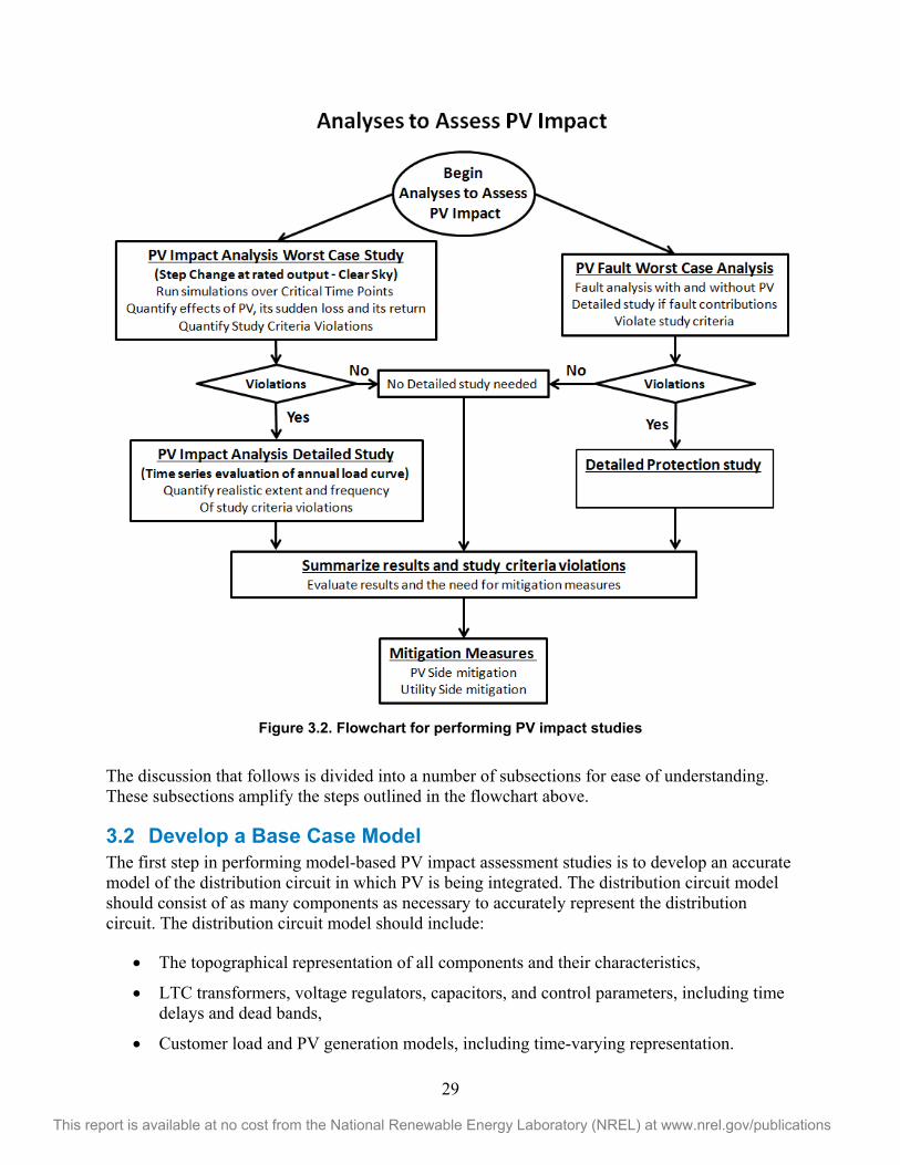
29
This report is available at no cost from the National Renewable Energy Laboratory (NREL) at www.nrel.gov/publications
Figure 3.2. Flowchart for performing PV impact studies
The discussion that follows is divided into a number of subsections for ease of understanding. These subsections amplify the steps outlined in the flowchart above.
3.2 Develop a Base Case Model The first step in performing model-based PV impact assessment studies is to develop an accurate model of the distribution circuit in which PV is being integrated. The distribution circuit model should consist of as many components as necessary to accurately represent the distribution circuit. The distribution circuit model should include:
The topographical representation of all components and their characteristics,
LTC transformers, voltage regulators, capacitors, and control parameters, including time delays and dead bands,
Customer load and PV generation models, including time-varying representation.
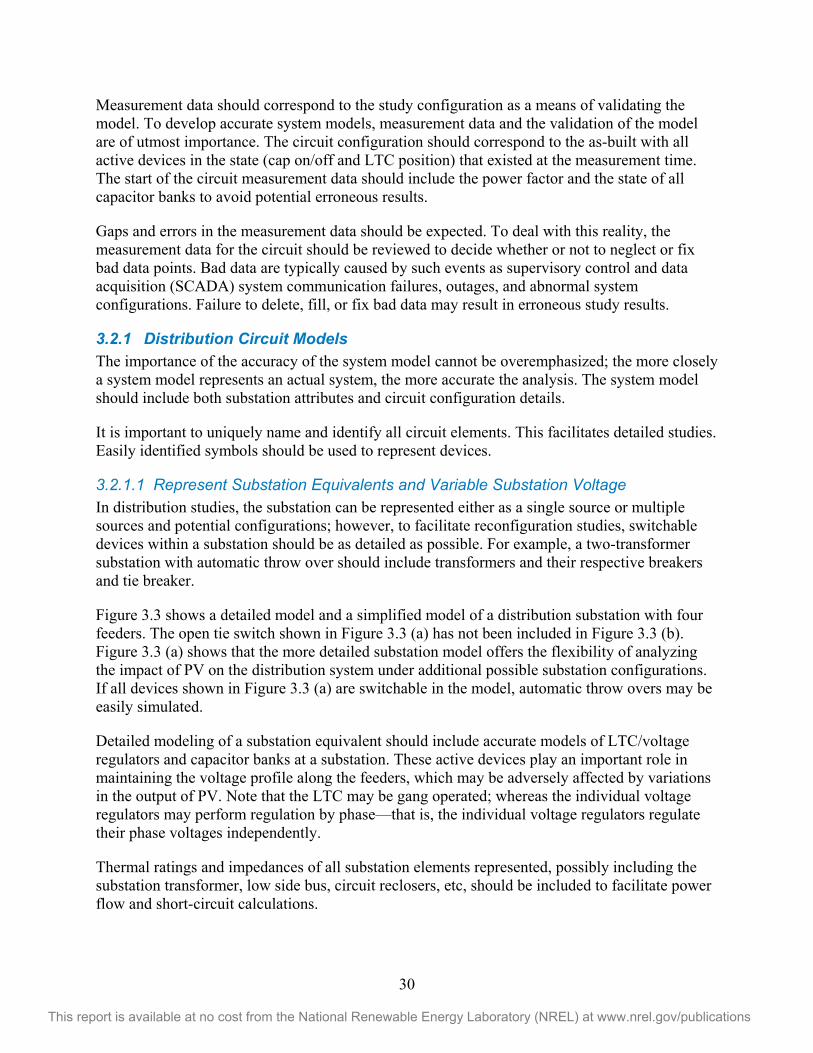
30
This report is available at no cost from the National Renewable Energy Laboratory (NREL) at www.nrel.gov/publications
Measurement data should correspond to the study configuration as a means of validating the model. To develop accurate system models, measurement data and the validation of the model are of utmost importance. The circuit configuration should correspond to the as-built with all active devices in the state (cap on/off and LTC position) that existed at the measurement time. The start of the circuit measurement data should include the power factor and the state of all capacitor banks to avoid potential erroneous results.
Gaps and errors in the measurement data should be expected. To deal with this reality, the measurement data for the circuit should be reviewed to decide whether or not to neglect or fix bad data points. Bad data are typically caused by such events as supervisory control and data acquisition (SCADA) system communication failures, outages, and abnormal system configurations. Failure to delete, fill, or fix bad data may result in erroneous study results.
3.2.1 Distribution Circuit Models The importance of the accuracy of the system model cannot be overemphasized; the more closely a system model represents an actual system, the more accurate the analysis. The system model should include both substation attributes and circuit configuration details.
It is important to uniquely name and identify all circuit elements. This facilitates detailed studies. Easily identified symbols should be used to represent devices.
3.2.1.1 Represent Substation Equivalents and Variable Substation Voltage In distribution studies, the substation can be represented either as a single source or multiple sources and potential configurations; however, to facilitate reconfiguration studies, switchable devices within a substation should be as detailed as possible. For example, a two-transformer substation with automatic throw over should include transformers and their respective breakers and tie breaker.
Figure 3.3 shows a detailed model and a simplified model of a distribution substation with four feeders. The open tie switch shown in Figure 3.3 (a) has not been included in Figure 3.3 (b). Figure 3.3 (a) shows that the more detailed substation model offers the flexibility of analyzing the impact of PV on the distribution system under additional possible substation configurations. If all devices shown in Figure 3.3 (a) are switchable in the model, automatic throw overs may be easily simulated.
Detailed modeling of a substation equivalent should include accurate models of LTC/voltage regulators and capacitor banks at a substation. These active devices play an important role in maintaining the voltage profile along the feeders, which may be adversely affected by variations in the output of PV. Note that the LTC may be gang operated; whereas the individual voltage regulators may perform regulation by phase—that is, the individual voltage regulators regulate their phase voltages independently.
Thermal ratings and impedances of all substation elements represented, possibly including the substation transformer, low side bus, circuit reclosers, etc, should be included to facilitate power flow and short-circuit calculations.
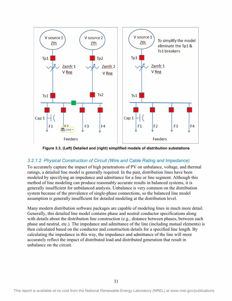
31
This report is available at no cost from the National Renewable Energy Laboratory (NREL) at www.nrel.gov/publications
Figure 3.3. (Left) Detailed and (right) simplified models of distribution substations
3.2.1.2 Physical Construction of Circuit (Wire and Cable Rating and Impedance) To accurately capture the impact of high penetrations of PV on unbalance, voltage, and thermal ratings, a detailed line model is generally required. In the past, distribution lines have been modeled by specifying an impedance and admittance for a line or line segment. Although this method of line modeling can produce reasonably accurate results in balanced systems, it is generally insufficient for unbalanced analysis. Unbalance is very common on the distribution system because of the prevalence of single-phase connections, so the balanced line model assumption is generally insufficient for detailed modeling at the distribution level.
Many modern distribution software packages are capable of modeling lines in much more detail. Generally, this detailed line model contains phase and neutral conductor specifications along with details about the distribution line construction (e.g., distance between phases, between each phase and neutral, etc.). The impedance and admittance of the line (including mutual elements) is then calculated based on the conductor and construction details for a specified line length. By calculating the impedance in this way, the impedance and admittance of the line will more accurately reflect the impact of distributed load and distributed generation that result in unbalance on the circuit.
32
This report is available at no cost from the National Renewable Energy Laboratory (NREL) at www.nrel.gov/publications
3.2.1.3 Automatic Voltage Regulation Equipment Models 3.2.1.3.1 Voltage Regulating Transformers—LTCs and Line Voltage Regulators A voltage regulating transformer (VRT) is a power transformer that can automatically change its turn ratio under load. Common ranges for VRT turns ratio adjustment are ±5% or ±10%, using 16 or 32 discreet steps or taps, respectively. VRT may be single phase or multiphase. Multiphase VRTs may be gang operated (all phases operate at the same time based on feedback from one phase), which is normally the case for substation transformer LTCs. Individual phases may be controlled independently, which is usually the case for voltage regulators within the feeder.
Typical control for a VRT includes a voltage set point and a control bandwidth. Based on local voltage feedback, the VRT changes its turn ratio to keep the load voltage within the range specified by the voltage set point and control bandwidth. In a typical radial circuit configuration, the load voltage is the side downstream from the substation.
In addition to the voltage set points, the VRT controller will typically include time delay settings. The VRT will delay operation until the monitored voltage is outside of the acceptable voltage range longer than the delay settings. When multiple voltage regulators are present on the circuit, distribution planners will typically coordinate VRT action by coordinating their time delays. An example of this is given in Figure 3.4 below.
Figure 3.4. Example of voltage regulators and control details
VRT control may also include line drop compensation to improve the voltage along the feeder. Line drop compensation is a way to simulate regulation at a nonlocal point based on local current and voltage feedback. To accomplish this, a VRT controller with line drop compensation typically includes an impedance setting (generally measured and set in volts). The VRT controller uses the impedance setting along with the local voltage at the VRT and the current through the VRT to estimate the voltage drop along the circuit. The VRT uses this estimated voltage drop to determine if a control action is needed.
A VRT with a line drop compensator can be used to improve the voltage as load varies. The line drop compensator senses line current. An increase in current will cause the output of the regulator to increase to a level higher than the set voltage. The compensator may raise the voltage of the regulator above 126 V, but it will keep the first customer below 126 V. This feature is often called the first house setting. A line that uses a compensator should be monitored.
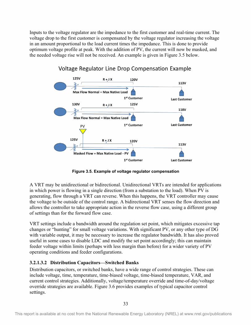
33
This report is available at no cost from the National Renewable Energy Laboratory (NREL) at www.nrel.gov/publications
Inputs to the voltage regulator are the impedance to the first customer and real-time current. The voltage drop to the first customer is compensated by the voltage regulator increasing the voltage in an amount proportional to the load current times the impedance. This is done to provide optimum voltage profile at peak. With the addition of PV, the current will now be masked, and the needed voltage rise will not be received. An example is given in Figure 3.5 below.
Figure 3.5. Example of voltage regulator compensation
A VRT may be unidirectional or bidirectional. Unidirectional VRTs are intended for applications in which power is flowing in a single direction (from a substation to the load). When PV is generating, flow through a VRT can reverse. When this happens, the VRT controller may cause the voltage to be outside of the control range. A bidirectional VRT senses the flow direction and allows the controller to take appropriate action in the reverse flow case, using a different group of settings than for the forward flow case.
VRT settings include a bandwidth around the regulation set point, which mitigates excessive tap changes or “hunting” for small voltage variations. With significant PV, or any other type of DG with variable output, it may be necessary to increase the regulator bandwidth. It has also proved useful in some cases to disable LDC and modify the set point accordingly; this can maintain feeder voltage within limits (perhaps with less margin than before) for a wider variety of PV operating conditions and feeder configurations.
3.2.1.3.2 Distribution Capacitors—Switched Banks Distribution capacitors, or switched banks, have a wide range of control strategies. These can include voltage, time, temperature, time-biased voltage, time-biased temperature, VAR, and current control strategies. Additionally, voltage/temperature override and time-of-day/voltage override strategies are available. Figure 3.6 provides examples of typical capacitor control settings.
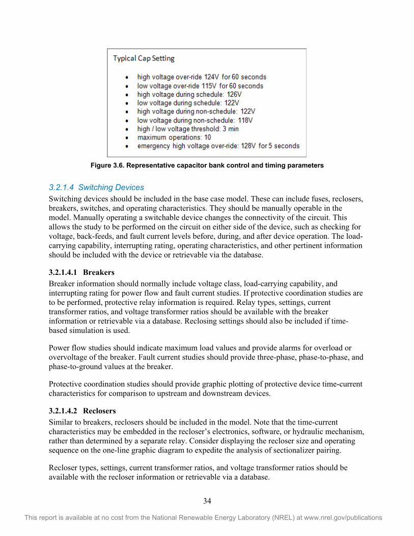
34
This report is available at no cost from the National Renewable Energy Laboratory (NREL) at www.nrel.gov/publications
Figure 3.6. Representative capacitor bank control and timing parameters
3.2.1.4 Switching Devices Switching devices should be included in the base case model. These can include fuses, reclosers, breakers, switches, and operating characteristics. They should be manually operable in the model. Manually operating a switchable device changes the connectivity of the circuit. This allows the study to be performed on the circuit on either side of the device, such as checking for voltage, back-feeds, and fault current levels before, during, and after device operation. The load-carrying capability, interrupting rating, operating characteristics, and other pertinent information should be included with the device or retrievable via the database.
3.2.1.4.1 Breakers Breaker information should normally include voltage class, load-carrying capability, and interrupting rating for power flow and fault current studies. If protective coordination studies are to be performed, protective relay information is required. Relay types, settings, current transformer ratios, and voltage transformer ratios should be available with the breaker information or retrievable via a database. Reclosing settings should also be included if time-based simulation is used.
Power flow studies should indicate maximum load values and provide alarms for overload or overvoltage of the breaker. Fault current studies should provide three-phase, phase-to-phase, and phase-to-ground values at the breaker.
Protective coordination studies should provide graphic plotting of protective device time-current characteristics for comparison to upstream and downstream devices.
3.2.1.4.2 Reclosers Similar to breakers, reclosers should be included in the model. Note that the time-current characteristics may be embedded in the recloser’s electronics, software, or hydraulic mechanism, rather than determined by a separate relay. Consider displaying the recloser size and operating sequence on the one-line graphic diagram to expedite the analysis of sectionalizer pairing.
Recloser types, settings, current transformer ratios, and voltage transformer ratios should be available with the recloser information or retrievable via a database.
35
This report is available at no cost from the National Renewable Energy Laboratory (NREL) at www.nrel.gov/publications
3.2.1.4.3 Fuses Load-carrying capability, interrupting rating, and time-current characteristics should be included with fuses. Because of the large number of fuses typically used in a circuit, it is typically helpful if the load-carrying capability in amperes and time-current curve can be easily shown on the one-line graphic diagram. For example: 65 K or 125 E 119.
3.2.1.4.4 Sectionlizers Sectionalizers are used to isolate sections of a circuit downstream of a recloser. The current-carrying capability and operating sequence should be included in the model. Typically, sectionalizers open after the current is interrupted by an upstream recloser. They normally do not interrupt fault current and have no interrupting rating. Consider displaying the sectionalizer and operating sequence on the one-line graphic diagram to expedite checking proper pairing with reclosers.
3.2.1.4.5 Switches All switches installed at the primary voltage (e.g., at 12.47-kV, 13.2-kV) level should be included in the model. They should have manual operability via the one-line graphic to expedite power flow and fault current studies for remaining portions of the circuit when the switch is open. Also consider including switches installed on the secondary voltage if it is expected that studies will be run when they are open. It is helpful to include load-carrying capability and notation of the type of switch—such as single phase, gang operated, SCADA controlled, or automatic—on the one-line graphic display.
3.2.1.5 Load Models—Varying Load Types and Calculating Native Load The feeder load distribution can be calculated using various types of individual customer load models. Ideally, the load models should be time varying (see section 3.3 Time Series Input—Develop Data Used to Inform the Models) . The system should be capable of performing a power flow for a specific date and time or a range of times.
Some commonly used sources for load information include:
Connected KVA—load is based on the distribution transformer capacity
Energy consumption—load is based on load research statistics and/or monthly usage obtained from monthly billing systems and can be used to develop time-varying loads. These load estimates are often broken down by load class for more accuracy. Billed monthly usage can be broken down by class and combined with typical load profiles provided from load research statistics. MV90 (¼- or ½-h)—demand measurements, typically for the larger customers
AMI—individual hourly demand measurements for every meter fed from a distribution transformer
SCADA or historical data—measured data taken from a historian for feeder head and other circuit elements.
Feeder load allocation based on connected kVA (load modeling based on the size of the transformer) can be used, but it is typically not very accurate. For example, if a 5 kVA
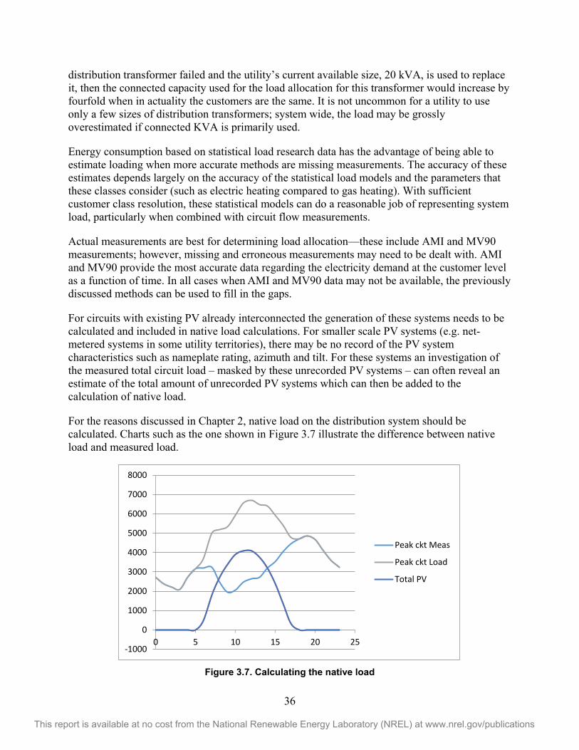
36
This report is available at no cost from the National Renewable Energy Laboratory (NREL) at www.nrel.gov/publications
distribution transformer failed and the utility’s current available size, 20 kVA, is used to replace it, then the connected capacity used for the load allocation for this transformer would increase by fourfold when in actuality the customers are the same. It is not uncommon for a utility to use only a few sizes of distribution transformers; system wide, the load may be grossly overestimated if connected KVA is primarily used.
Energy consumption based on statistical load research data has the advantage of being able to estimate loading when more accurate methods are missing measurements. The accuracy of these estimates depends largely on the accuracy of the statistical load models and the parameters that these classes consider (such as electric heating compared to gas heating). With sufficient customer class resolution, these statistical models can do a reasonable job of representing system load, particularly when combined with circuit flow measurements.
Actual measurements are best for determining load allocation—these include AMI and MV90 measurements; however, missing and erroneous measurements may need to be dealt with. AMI and MV90 provide the most accurate data regarding the electricity demand at the customer level as a function of time. In all cases when AMI and MV90 data may not be available, the previously discussed methods can be used to fill in the gaps.
For circuits with existing PV already interconnected the generation of these systems needs to be calculated and included in native load calculations. For smaller scale PV systems (e.g. net-metered systems in some utility territories), there may be no record of the PV system characteristics such as nameplate rating, azimuth and tilt. For these systems an investigation of the measured total circuit load – masked by these unrecorded PV systems – can often reveal an estimate of the total amount of unrecorded PV systems which can then be added to the calculation of native load.
For the reasons discussed in Chapter 2, native load on the distribution system should be calculated. Charts such as the one shown in Figure 3.7 illustrate the difference between native load and measured load.
Figure 3.7. Calculating the native load
-1000
0
1000
2000
3000
4000
5000
6000
7000
8000
0 5 10 15 20 25
Peak ckt Meas
Peak ckt Load
Total PV
37
This report is available at no cost from the National Renewable Energy Laboratory (NREL) at www.nrel.gov/publications
The total for the feeder flow can be summed from the estimates of the individual load points and then compared to the measured start of circuit. Scaling can be done to resolve the difference between the metered flow and the sum of the estimated feeder loads and losses. If large scaling factors are noted, it is advised to check the model’s configuration of the circuit to ensure that it corresponds to the configuration for which the start-of-circuit measurements were taken.
Note that when using customer load information, metered data is generally considered to be more reliable than billing data. For example, it is not uncommon for billing data to include estimated consumption data or make-up readings (if a meter reading is skipped). Another example is individual hourly demands from MV90, in which the billing information may be for consumption during the period with a monthly average power factor. This represents a loss of fidelity which will typically result in lower confidence in the modeling results. An important example in the case of PV adoption studies is a net metered customer. This customer’s consumption for a period might actually be zero if the PV output were high enough. Such masked native load will be a recurring problem.
3.2.2 PV System Models 3.2.2.1 Single Utility-Scale PV System A single utility-scale PV plant is typically three phase and 1 MW or larger. Larger three-phase units typically require one or more interconnection transformers and include several inverters connected in parallel. Each of the inverters is equipped with its own protection systems. This typically includes fast overcurrent protection, over-/undervoltage and frequency, and anti-islanding protection schemes. A single PV system consisting of multiple inverters may act as one unit from a study perspective. This is particularly true if the PV system is contiguous and occupies a relatively small footprint.
3.2.2.2 Multiple Utility-Scale PV Systems in Near Proximity Multiple PV systems may exist on a distribution circuit. Depending on their proximity to each other, they may act together. For example, output variability because of fast-moving clouds may affect the output from multiple PV units as if they were one unit producing voltage rise and fall issues. Fault currents, depending on configuration, may be additive.
3.2.2.3 PV Inverters The IEEE 1547 series of standards deals with the interconnection of DG on the distribution system. Although the series is not specific to PV, much of the content of the series applies to distributed PV.
At the time of publication, the 1547 series contains the base standards along with six guides and recommended practices. These standards are as follows:
1547a-2014—IEEE Standard for Interconnecting Distributed Resources with Electric Power Systems
1547.1-2005—IEEE Standard Conformance Test Procedures for Equipment Interconnecting Distributed Resources with Electric Power Systems
38
This report is available at no cost from the National Renewable Energy Laboratory (NREL) at www.nrel.gov/publications
1547.2-2008—IEEE Application Guide for IEEE Standard 1547, IEEE Standard for Interconnecting Distributed Resources with Electric Power Systems
1547.3-2007—IEEE Guide For Monitoring, Information Exchange, and Control of Distributed Resources Interconnected with Electric Power Systems
1547.4-2011—IEEE Guide for Design, Operation, and Integration of Distributed Resource Island Systems with Electric Power Systems
1547.6-2011—IEEE Recommended Practice For Interconnecting Distributed Resources with Electric Power Systems Distribution Secondary Networks
1547.7-2013—IEEE Guide for Conducting Distribution Impact Studies for Distributed Resource Interconnection.
In addition to the published standards, the series contains the IEEE P1547.8—IEEE Draft Recommended Practice for Establishing Methods and Procedures that Provide Supplemental Support for Implementation Strategies for Expanded Use of IEEE 1547, which is under development. Additionally, in 2013 a working group was formed to consider revising the base standard, IEEE 1547.
The base standard is written from the perspective of the point of common coupling, which is generally the interconnection point between a utility system and the DG’s local electrical system (which may contain multiple types of DG). The standards contain specifications for how DG (or colocated and interconnected groups of DG) should operate during normal and abnormal grid conditions.
Because the focus of 1547 is on the point of common coupling, the base standards do not comprehensively apply to high-penetration PV scenarios (which are a system-level concern). Additionally, the relative novelty of DG when the base standards were originally written has called into question the compatibility of the base standards as levels of DG continue to rise. Most concerns about the base standards relate to the response of the DG to abnormal conditions and the flexibility of the DG to regulate voltage. To address these concerns, the base standard was amended in 2013 to relax its stance on voltage regulation and voltage and frequency ride-through.
3.2.2.3.1 Smart Inverter Functions The following smart inverter control algorithms, per the Electric Power Research Institute smart inverter functions, could be included in the PV model, particularly to enable mitigation, if required. This list is not exhaustive but provides the smart inverter functions being used currently or believed to be used in the near future:
Priority setting
PV setting modification
Power factor adjustment
Low-voltage ride-through/high-voltage ride-through
Volt-watt control
39
This report is available at no cost from the National Renewable Energy Laboratory (NREL) at www.nrel.gov/publications
Dynamic reactive current support
Intelligent volt-var control
Note that the low-voltage ride-through and high-voltage ride-through functionalities will require interfacing to network fault calculations.
The following are descriptions of the smart inverter controls.
3.2.2.3.2 Priority Setting During normal operation, the reactive power control is accomplished whenever the real power generation is less than its rated power level so that the real power generation has the higher priority; however, if the utility needs to control the reactive power by reducing the real power generation, an inverter can be programmed to set the reactive power control to a higher priority. This mode can be used for feeders with voltage flicker issues.
3.2.2.3.3 PV Setting Modification The maximum power and reactive power capacities can be limited by PV setting modification. This function is designed to let the utility limit the capacities to provide a stable voltage regulation range or provide more reactive power control capability to regulate the line voltage.
3.2.2.3.4 Power Factor Adjustment An inverter’s output power factor can be controlled within the limit of the available reactive current. This mode can be used to limit the operating alternating-current (AC) voltage within the allowable levels. Time window and ramp rate can be configured as options. The response time can be programmed with a range of 300 ms to several seconds with ramp rate option settings.
Injecting real power (watts) or reactive power (vars) will increase the voltage at the point of injection; conversely, absorbing real or reactive power will decrease the voltage. By operating the PV at an absorbing power factor, the PV will absorb more reactive power as the real power output increases. This will help mitigate the increase in voltage with increases in real power injection.
3.2.2.3.5 Low-Voltage Ride-Through/High-Voltage Ride-Through With conventional grid operations, distribution line faults may cause cascading failures. PV inverters can be used to actively mitigate the transient caused by power line failures and prevent secondary breakdowns. Set points and time durations of at least four different operating modes can be customized and will be reserved for flexible configurations needed for different utility requirements.
The following list illustrates maximum voltage ride-through conditions:
V > 120%—must disconnect
115% < V < 120%—500 ms
110% < V < 115%—1 s
88% < V < 110%—remain connected

40
This report is available at no cost from the National Renewable Energy Laboratory (NREL) at www.nrel.gov/publications
65% < V < 88%—3 s
50% < V < 65%—300 ms
V < 50%—must disconnect
3.2.2.3.6 Volt-Watt Control When a distribution line has high resistance, the AC voltage can be regulated with the real power. This control can be used to limit the AC voltage magnitude within the normal operating range. Similar to volt-VAR control, described below, the volt-watt curve can be programmed with optional hysteresis and dead band.
Distribution line-specific operating conditions can be configured using available modes. The response time can be programmed with a range of 300 ms to several seconds with ramp rate option settings.
3.2.2.3.7 Dynamic Reactive Current Support Voltage flicker can be controlled with the fast dynamic response of the inverter. The response time will be as fast as 100 ms. This operation is designed to respond to the AC voltage fluctuation for the short duration caused by load changes or line disturbances. The dynamic reactive current support curve can be programmed with optional hysteresis and dead band. This mode can be operated in conjunction with the priority setting to regulate AC voltage.
3.2.2.3.8 Intelligent Volt-VAR Control The distribution line voltage can be regulated within an inverter’s available power capacity. The AC voltage control can be coordinated at the SCADA level with other ancillary control equipment, such as capacitor banks or voltage regulators. The volt-VAR curve can be programmed with optional hysteresis and dead band. Distribution line-specific operating conditions can be configured using available modes. The response time can be programmed to be between 300 ms and several seconds with the ramp rate option setting.
3.2.2.4 Fault Current PV Models Fault current models are considered current source models and generally have a maximum fault current contribution of 1.1 or 1.2 times full load current until an inverter’s protection system operates. The timing at minimum should be that as outlined in the IEEE 1547 requirements. Manufacture specifications should provide exact details.
3.3 Time Series Input—Develop Data Used to Inform the Models 3.3.1 Utility SCADA Data (Synchronizing Data and Navigating the Issues) Data available through SCADA measurements can be used to model load and PV and also to verify the accuracy of the analysis results. It is important to ensure that the SCADA data are synchronized—i.e., the data used for developing the load and PV models or validating the analysis results should correspond to the same time period and feeder configuration.
41
This report is available at no cost from the National Renewable Energy Laboratory (NREL) at www.nrel.gov/publications
3.3.1.1 Substation-Level Data Start-of-feeder measurements can provide a significant increase in the accuracy of the study results. Typical SCADA time interval measurements for the start of feeder should be sufficient. A minimum measurement set for start-of-feeder measurements should include peak load and minimum daytime load throughout the annual operation. If 1-min or 1-s data are available, they can be used in the quasi-steady-state analysis for detailed studies when necessary. Also often included in SCADA time-interval measurements are switched capacitor bank status, LTC tap setting and VRT tap setting, which are invaluable for model validation and circuit operation evaluation.
3.3.1.2 PV System-Level Data When performing a PV assessment study, one year or more of PV generation measurement data should ideally be used. Whenever possible, the sampling rate should be faster than the operating times of voltage regulation equipment used on the circuit (typically on the order of 30 s or longer) to determine voltage regulation issues. In general, PV impact analysis becomes more accurate as the sampling rate of the PV generation increases. A 1 s sampling rate is preferred.
PV measurement data can be normalized by developing a solar profile for one system and scaling it appropriately to be used for other new and existing systems in the same region. Generation metering, radiant metering, and temporary metering sources can provide high-fidelity measurement data.
3.3.1.3 Other Circuit-Level Data Additional metering data sources may also exist on the distribution circuit, such as relays, reclosers, remotely controlled pole switches, voltage regulators, and temporary metering, such as the GridSense LineTracker meters, which were used to validate the circuit flows in Example 1 in this handbook (Section 3.7).
3.3.2 Modeled PV Power Output Data (with existing PV Plant Data) When SCADA measurements for PV are unavailable, a number of other techniques and resources can be used to develop a solar generation profile for PV impact analysis. For these techniques, the minimum PV data needed are the geographical location (latitude and longitude are ideal) and size of the generator. Additional data that support more precise analysis include:
Azimuth and tilt of the solar panels
Inverter efficiencies
Inverter power factor
Inverter control strategy
When the data above are not available the generally accepted conservative practice to assume PV power output at 100% of the PV inverter(s) nameplate with a power factor equal to unity.
A number of free (e.g., National Renewable Energy Laboratory) and paid (e.g., Clean Power Research and Forecasting and IBM) resources are available on the Internet from which PV
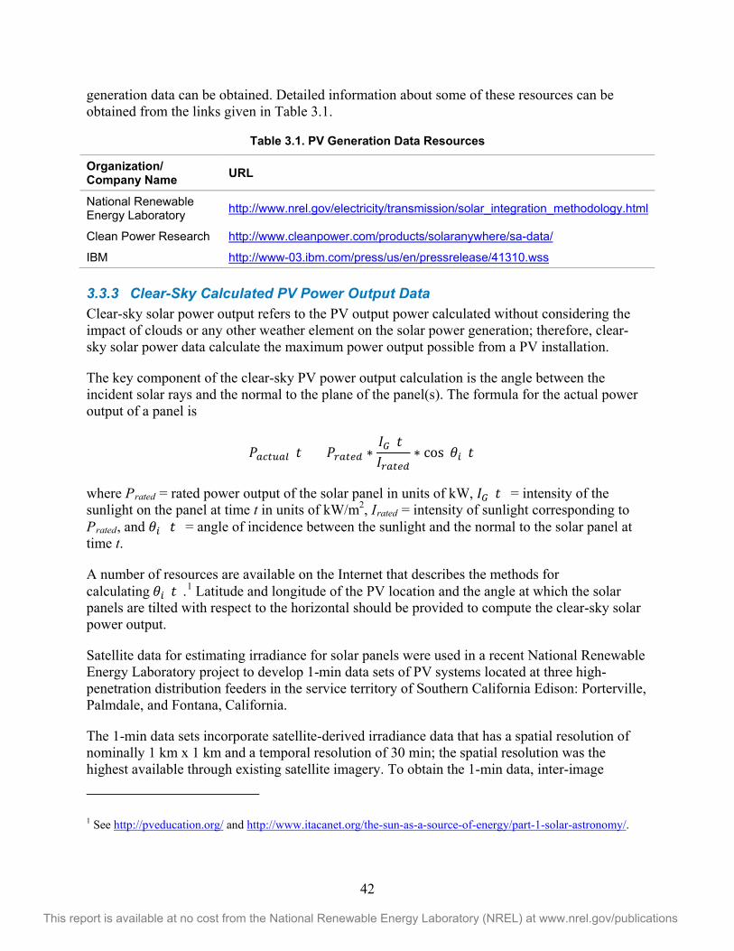
42
This report is available at no cost from the National Renewable Energy Laboratory (NREL) at www.nrel.gov/publications
generation data can be obtained. Detailed information about some of these resources can be obtained from the links given in Table 3.1.
Table 3.1. PV Generation Data Resources
Organization/ Company Name URL
National Renewable Energy Laboratory http://www.nrel.gov/electricity/transmission/solar_integration_methodology.html
Clean Power Research http://www.cleanpower.com/products/solaranywhere/sa-data/
IBM http://www-03.ibm.com/press/us/en/pressrelease/41310.wss
3.3.3 Clear-Sky Calculated PV Power Output Data Clear-sky solar power output refers to the PV output power calculated without considering the impact of clouds or any other weather element on the solar power generation; therefore, clear-sky solar power data calculate the maximum power output possible from a PV installation.
The key component of the clear-sky PV power output calculation is the angle between the incident solar rays and the normal to the plane of the panel(s). The formula for the actual power output of a panel is
( ) =( )
cos ( ( ))
where Prated = rated power output of the solar panel in units of kW, ( ) = intensity of the sunlight on the panel at time t in units of kW/m2, Irated = intensity of sunlight corresponding to Prated, and ( ) = angle of incidence between the sunlight and the normal to the solar panel at time t.
A number of resources are available on the Internet that describes the methods for calculating ( ).1 Latitude and longitude of the PV location and the angle at which the solar panels are tilted with respect to the horizontal should be provided to compute the clear-sky solar power output.
Satellite data for estimating irradiance for solar panels were used in a recent National Renewable Energy Laboratory project to develop 1-min data sets of PV systems located at three high-penetration distribution feeders in the service territory of Southern California Edison: Porterville, Palmdale, and Fontana, California.
The 1-min data sets incorporate satellite-derived irradiance data that has a spatial resolution of nominally 1 km x 1 km and a temporal resolution of 30 min; the spatial resolution was the highest available through existing satellite imagery. To obtain the 1-min data, inter-image
1 See http://pveducation.org/ and http://www.itacanet.org/the-sun-as-a-source-of-energy/part-1-solar-astronomy/.
43
This report is available at no cost from the National Renewable Energy Laboratory (NREL) at www.nrel.gov/publications
interpolations were generated with a “cloud motion vector” method by translating the previous image over time using wind speed and direction. The resulting irradiance data were fed into a PV simulation model to produce power output.
While 1 minute temporal resolution data was developed specifically for the above mentioned project, similar data sets at lower temporal resolutions are more easily available. Through such data sets, utility engineers can model the power output of PV more accurately and better predict the impacts of high-penetration PV on their distribution circuits.
3.4 Validate Time Series Measurement Data Gaps and errors in the measurement data should be expected. To deal with this reality, the measurement data should be reviewed to decide whether to neglect or to fix bad data points. Bad data are typically caused by such events as SCADA communication failures, outages, and abnormal system configurations. Failure to delete, fill, or fix bad data may result in erroneous impact study results. It may be helpful to obtain a listing of outages and or switching times to help discover data that do not apply to the normal system. In addition, the velocity of the measurement changes can be used to discover bad data. Detecting missing data, detecting bad data, and fixing these using tools such as Excel and Access are addressed in Appendix A.
3.4.1 Validate Circuit Model Calibration and validation of the model is accomplished by verifying that the native load on the system closely matches the SCADA data in magnitude over time. If available, the operation of the voltage regulation equipment on the circuit is compared between the modeled circuit and the observed operation of the equipment to verify the validity of the modeled voltage regulation equipment control methods and set points.
3.4.2 Add Measurements Determine the measurement times to use in the validation process from the measurement set (e.g., peak load time, light load time, maximum PV generation time).
3.4.3 Run Power Flow Run power flow at the selected times to determine if there is a close match between the sum of the customer loads and the SCADA measurements. If a large mismatch is noted (i.e. error is greater than 5-10%), the model should be investigated for correctness.
3.5 Determine Quasi-Steady-State Critical Time Points and Study Criteria
After the circuit model is built and validated, it is then possible to identify the minimum and maximum daytime load points. To do this, all of the PV generation, including estimates for existing PV on the circuit, in the model should be turned off, and a full hourly power flow simulation (8,760 individual power flow solutions) should be performed. Post processing these results allows for the identification of the global minima and maxima at the feeder level. Then PV measurements may be used with the time-varying load to determine other critical time points, such as maximum PV generation and maximum difference between load and PV generation during the time of PV generation.
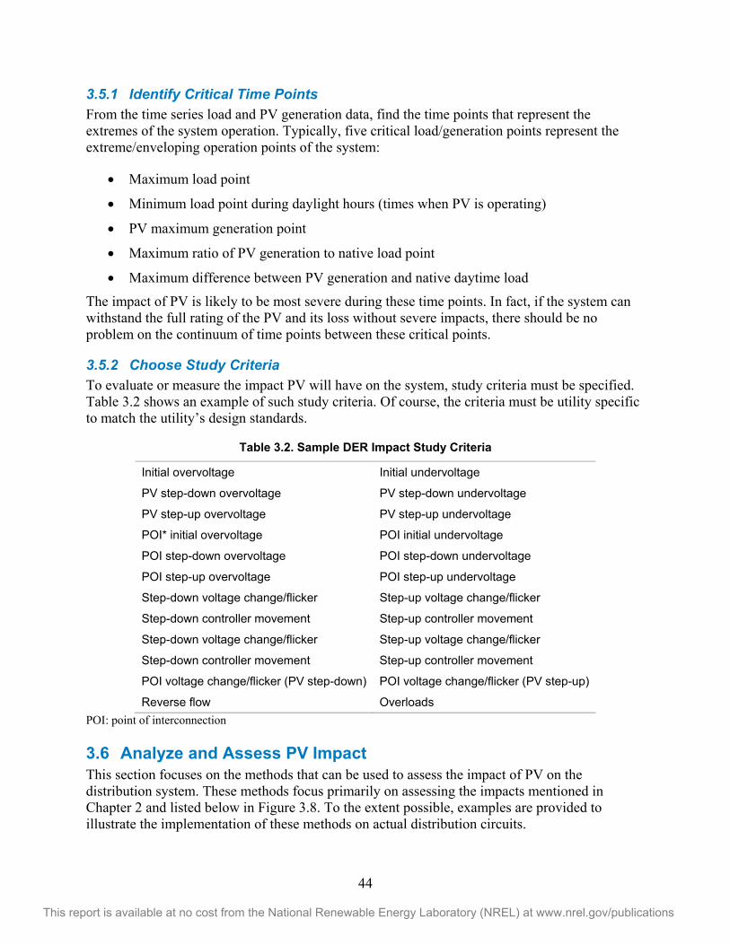
44
This report is available at no cost from the National Renewable Energy Laboratory (NREL) at www.nrel.gov/publications
3.5.1 Identify Critical Time Points From the time series load and PV generation data, find the time points that represent the extremes of the system operation. Typically, five critical load/generation points represent the extreme/enveloping operation points of the system:
Maximum load point
Minimum load point during daylight hours (times when PV is operating)
PV maximum generation point
Maximum ratio of PV generation to native load point
Maximum difference between PV generation and native daytime load
The impact of PV is likely to be most severe during these time points. In fact, if the system can withstand the full rating of the PV and its loss without severe impacts, there should be no problem on the continuum of time points between these critical points.
3.5.2 Choose Study Criteria To evaluate or measure the impact PV will have on the system, study criteria must be specified. Table 3.2 shows an example of such study criteria. Of course, the criteria must be utility specific to match the utility’s design standards.
Table 3.2. Sample DER Impact Study Criteria
Initial overvoltage Initial undervoltage
PV step-down overvoltage PV step-down undervoltage
PV step-up overvoltage PV step-up undervoltage
POI* initial overvoltage POI initial undervoltage
POI step-down overvoltage POI step-down undervoltage
POI step-up overvoltage POI step-up undervoltage
Step-down voltage change/flicker Step-up voltage change/flicker
Step-down controller movement Step-up controller movement
Step-down voltage change/flicker Step-up voltage change/flicker
Step-down controller movement Step-up controller movement
POI voltage change/flicker (PV step-down) POI voltage change/flicker (PV step-up)
Reverse flow Overloads POI: point of interconnection 3.6 Analyze and Assess PV Impact This section focuses on the methods that can be used to assess the impact of PV on the distribution system. These methods focus primarily on assessing the impacts mentioned in Chapter 2 and listed below in Figure 3.8. To the extent possible, examples are provided to illustrate the implementation of these methods on actual distribution circuits.
45
This report is available at no cost from the National Renewable Energy Laboratory (NREL) at www.nrel.gov/publications
The PV assessment is divided into two paths to evaluate the impacts of PV generation on distribution circuits, and they include the various adverse effects that DG may have, as follows:
Power flow—Analyzes power flow and voltage level on the system with and without PV
o Worst-case step-change analysis—Analyzes worst-case variations in PV at critical time points
o Detailed study
Step change—Analyzes variation in PV at critical time points
Controller movement—Estimates system controller movements with and without PV
Variability analysis—Examines step changes in PV generation
Fault analysis—Analyzes the system protection elements with and without PV
o Fault analysis—Analyzes the worst-case system protection elements with and without PV
o Detailed protection study
Figure 3.8 provides a representative flow diagram of a PV impact study after the base case study system is developed. As illustrated, two study paths need to be pursued:
1. Power flow assessment
2. Network fault assessment
In each path, a preliminary assessment is compared to the chosen study criteria to reveal whether a problem exists. If problems are noted in either of the paths, a more specific study is needed to determine the exact impact and develop a realistic solution.
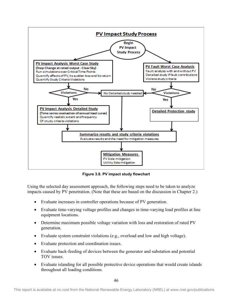
46
This report is available at no cost from the National Renewable Energy Laboratory (NREL) at www.nrel.gov/publications
Figure 3.8. PV impact study flowchart
Using the selected day assessment approach, the following steps need to be taken to analyze impacts caused by PV penetration. (Note that these are based on the discussion in Chapter 2.)
Evaluate increases in controller operations because of PV generation.
Evaluate time-varying voltage profiles and changes in time-varying load profiles at line equipment locations.
Determine maximum possible voltage variation with loss and restoration of rated PV generation.
Evaluate system constraint violations (e.g., overload and low and high voltage).
Evaluate protection and coordination issues.
Evaluate back-feeding of devices between the generator and substation and potential TOV issues.
Evaluate islanding for all possible protective device operations that would create islands throughout all loading conditions.
47
This report is available at no cost from the National Renewable Energy Laboratory (NREL) at www.nrel.gov/publications
3.6.1 Assess PV Using Power Flow Analysis The step-change analysis is used to evaluate the response of the circuit to the coordinated step change of output power at one or more PV sites. After the circuit model has been built and validated, the circuit is ready for this analysis. In this first step, the output power of a specified PV or group of PV systems (in near proximity) may be moved in unison and considered for adverse effects on conditions such as the system voltage, voltage controller movement, flicker, and reverse flows, among others. The full list of tested impact criteria is given in Appendix B.
3.6.1.1 Introduction There is a tradeoff between the accuracy of PV impact assessments and the data computations required for performing such assessments. Although performing annual assessments using data at 1-min intervals can provide very accurate results, these require running 1,051,200 power flows, which take up considerable computational and storage resources. Further, it may not be very useful to analyze all days of a year; instead, if a handful of critical days can provide the information necessary for a utility to effectively plan to address the impacts of high PV penetration, significant savings in time, effort, and resources can be achieved. The critical days for which quasi-static time series analysis can be performed can be identified as those containing the critical time points listed in Section 3.5.1. This list of critical days is not necessarily prescriptive, and a utility may increase or decrease the number of critical days for performing a PV impact assessment.
3.6.1.2 Methodology To assess the impact of PV on voltage and thermal loading of equipment in the distribution system, a series of power flow analysis runs are performed associated with loss and restoration of user-selected PV generation and corresponding load conditions. These include:
Base condition—distribution system with new PV
Loss of generation without feeder controls operating
Loss of generation with feeder controls operating
Return of generation without feeder controls operating
Return of generation with feeder controls operating
A series of loss-of-generation and return-of-generation percentages can be implemented in each power flow run to find the percentage of PV output that causes a voltage or thermal loading criteria violation to occur. Inverter power factor set points can also be varied to determine whether they can help address voltage and thermal loading violations. (See more about this in Chapter 4.)
The above power flow runs can also provide useful information about control device movements, back-feeds, percentage power imbalances, and percentage voltage imbalances. Information about percentage power and voltage imbalances can be particularly useful for areas in which larger amounts of single-phase PV may be present. Evaluating the percentage imbalance may serve as a utility mitigation measure when phase balancing on PV generation is used. Similarly, sections of the circuit in which solar generation results in back-feed or reverse power flow are vulnerable to
48
This report is available at no cost from the National Renewable Energy Laboratory (NREL) at www.nrel.gov/publications
voltage regulation issues. In addition, these may lead to transient overvoltages, as discussed in Chapter 2, and the need to perform a detailed dynamic study.
3.6.1.3 Worst-Case Study The first step is to run a series of power flows at each of the enveloping or critical time points. Examining the PV effect on the system at the system extremes while the PV is at its extremes is a way to bracket the potential problems in the hopes that the worst-case evaluation does not result in adverse circuit impacts. In most cases, if a system can operate at the extremes without adverse impacts, the interconnection of high-penetration PV is acceptable. If a study criteria violation is noted, a more detailed analysis should be undertaken.
3.6.1.4 Detailed Study A detailed study consists of running the same series of power flows at the critical time points using a variety of more realistic variability step changes to more accurately determine the extent of the study criteria violations.
Any power flow study issues should be summarized and combined with protection issues. Chapter 4 presents techniques for mitigating these issues.
3.6.2 Assess PV Using Fault Analysis 3.6.2.1 Introduction Fault analysis for circuits with PV connected is similar to analysis of circuits with synchronous or induction generation connected. Because the PV is usually connected to the utility via an inverter, the PV model is a current source, and parameters such as subtransient, transient, and synchronous reactance do not apply.
The proposed PV is added to the circuit model, and typical checks are made to ensure that interrupting ratings remain adequate, fault sensing is not degraded, and selectivity is maintained between all pairs of devices. Also, the possibility of islanding resulting in transient or TOV is checked. Similar to studies with synchronous generation, automatic reclosing practices need to be reviewed to ensure that breakers and reclosers are not automatically reclosed out of synchronism with any generation still online.
Note that the load-carrying capability of the protective devices should also be checked. This may require results from the power flow analysis.
3.6.2.2 Methodology Fault analysis evaluates the effects on fault currents that result from the addition of new PV generation. For the fault analysis, all generation on the feeder (including new generation) is operated at rated output. Two cases are associated with generation fault analysis:
1. Generation fault analysis base case—without new PV
2. Generation fault analysis new generation
It should not be necessary to consider variations in solar irradiance for the initial analysis. If problems are noted because of increased fault current, it may be worthwhile to determine the more accurate fault currents using PV power output from maximum solar irradiance rather than
49
This report is available at no cost from the National Renewable Energy Laboratory (NREL) at www.nrel.gov/publications
by assuming rated output. A fault current screening criterion that is often used is the 10% rule—that is, if the PV fault current at the point of interconnection (POI) is less than 10% of the system available fault current, protection should generally not be an issue. Usually system protection is applied with a considerable margin to ensure correct operation, and a 10% increase at the POI is not likely to erase the margin; however, if interrupting ratings, fault sensing, and selectivity are already marginal for certain points in the circuit, a detailed analysis should be performed to ensure selectivity. The practice for some utilities may differ, but detailed studies may be required. In all cases, the authority responsible for protective practices should review and approve any change in methods used to screen PV fault current criteria.
3.6.2.3 Detailed Study A detailed study consists of running a series of fault analyses, as described in Chapter 2. For convenience, these are restated as follows:
Fault current and interrupting rating
Fault sensing
Desensitizing the substation relay
Line-to-ground utility-system overvoltage
Nuisance fuse blowing
Reclosing out of synchronism
Islanding
Sectionalizer miscount
Reverse power relay operation—malfunctions on secondary networks
Reverse power relay operation—substation
Cold load pickup with and without PV
Faults within a PV zone
Isolating PV for an upstream fault
Fault causing voltage sag and tripping PV
Distribution automation studies and reconfiguration
Any protection issues should be summarized and combined with power flow study issues. Chapter 4 presents techniques for mitigating these impacts.
3.7 Porterville Example—PV Assessment The Porterville PV assessment study was made using DEW’s automated DER assessment application to determine the impacts of adding DER to the system. The application dialog is shown below.
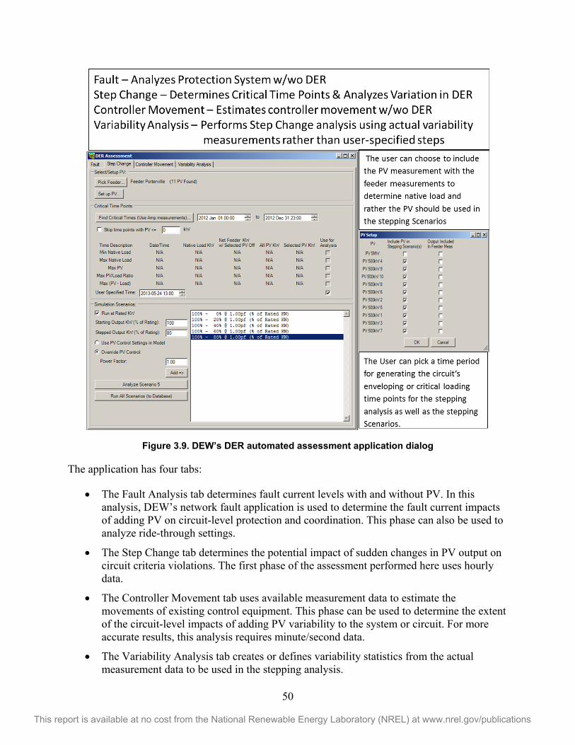
50
This report is available at no cost from the National Renewable Energy Laboratory (NREL) at www.nrel.gov/publications
Figure 3.9. DEW’s DER automated assessment application dialog
The application has four tabs:
The Fault Analysis tab determines fault current levels with and without PV. In this analysis, DEW’s network fault application is used to determine the fault current impacts of adding PV on circuit-level protection and coordination. This phase can also be used to analyze ride-through settings.
The Step Change tab determines the potential impact of sudden changes in PV output on circuit criteria violations. The first phase of the assessment performed here uses hourly data.
The Controller Movement tab uses available measurement data to estimate the movements of existing control equipment. This phase can be used to determine the extent of the circuit-level impacts of adding PV variability to the system or circuit. For more accurate results, this analysis requires minute/second data.
The Variability Analysis tab creates or defines variability statistics from the actual measurement data to be used in the stepping analysis.

51
This report is available at no cost from the National Renewable Energy Laboratory (NREL) at www.nrel.gov/publications
The following first discusses the step-change analysis, then the controller movement analysis, PV variability, and finally the fault analysis.
To determine the impact of adding PV to the circuit, the study considered the entire PV system acting as one from a solar variability perspective. Note that the DER assessment automatically combines the time-series start-of-circuit data and the coincident PV output to determine the circuit’s native load. The native load is then used to determine the critical load points for further analysis. All power flow results are written to a database and output into a report that takes into account the predetermined study criteria.
Detailed study results can be found in NREL/SCE High Penetration PV Integration Project: FY13 Annual Report (Mather et al. 2014). An overview of the study results are given below.
3.7.1 Developing the System Model The existing Porterville distribution circuit is 12 kV and approximately 40.7 mi in length. The planned peak load is 4,600 kW for its 442 customers. The circuit has four overhead switched capacitors and 5 MW of installed PV along a circuit length of approximately 2.6 miles. SCADA metering is available at the circuit head, and temporary metering (National Renewable Energy Laboratory distribution monitoring unit and GridSense LT40) has been installed as well. This additional high-speed monitoring was installed to obtain more granular measurement data and help ensure that the load allocation, which was made on connected capacity, was reasonable for the study. Circuit voltage regulation is provided by four overhead capacitor banks. Protection is provided by the substation breaker. See Figure 3.10.
Figure 3.10. Map of the Porterville circuit
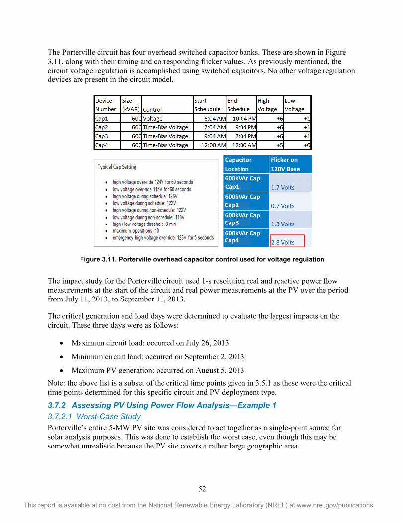
52
This report is available at no cost from the National Renewable Energy Laboratory (NREL) at www.nrel.gov/publications
The Porterville circuit has four overhead switched capacitor banks. These are shown in Figure 3.11, along with their timing and corresponding flicker values. As previously mentioned, the circuit voltage regulation is accomplished using switched capacitors. No other voltage regulation devices are present in the circuit model.
Figure 3.11. Porterville overhead capacitor control used for voltage regulation
The impact study for the Porterville circuit used 1-s resolution real and reactive power flow measurements at the start of the circuit and real power measurements at the PV over the period from July 11, 2013, to September 11, 2013.
The critical generation and load days were determined to evaluate the largest impacts on the circuit. These three days were as follows:
Maximum circuit load: occurred on July 26, 2013
Minimum circuit load: occurred on September 2, 2013
Maximum PV generation: occurred on August 5, 2013
Note: the above list is a subset of the critical time points given in 3.5.1 as these were the critical time points determined for this specific circuit and PV deployment type.
3.7.2 Assessing PV Using Power Flow Analysis—Example 1 3.7.2.1 Worst-Case Study Porterville’s entire 5-MW PV site was considered to act together as a single-point source for solar analysis purposes. This was done to establish the worst case, even though this may be somewhat unrealistic because the PV site covers a rather large geographic area.
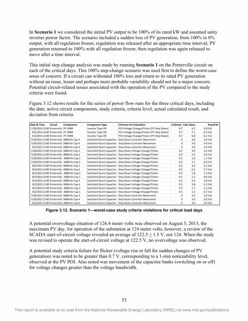
53
This report is available at no cost from the National Renewable Energy Laboratory (NREL) at www.nrel.gov/publications
In Scenario 1 we considered the initial PV output to be 100% of its rated kW and assumed unity inverter power factor. The scenario included a sudden loss of PV generation, from 100% to 0% output, with all regulation frozen; regulation was released after an appropriate time interval; PV generation returned to 100% with all regulation frozen; then regulation was again released to move after a time interval.
This initial step-change analysis was made by running Scenario 1 on the Porterville circuit on each of the critical days. This 100% step-change scenario was used first to define the worst-case areas of concern. If a circuit can withstand 100% loss and return to its rated PV generation without an issue, lesser and perhaps more probable variability should not be a major concern. Potential circuit-related issues associated with the operation of the PV compared to the study criteria were found.
Figure 3.12 shows results for the series of power flow runs for the three critical days, including the date, active circuit components, study criteria, criteria level, actual calculated result, and deviation from criteria.
Figure 3.12. Scenario 1—worst-case study criteria violations for critical load days
A potential overvoltage situation of 126.4 meter volts was observed on August 5, 2013, the maximum PV day, for operation of the substation at 124 meter volts; however, a review of the SCADA start-of-circuit voltage revealed an average of 122.5 + 1.5 V, not 124. When the study was revised to operate the start-of-circuit voltage at 122.5 V, no overvoltage was observed.
A potential study criteria failure for flicker (voltage rise or fall for sudden changes of PV generation) was noted to be greater than 0.7 V, corresponding to a 1-min noticeability level, observed at the PV POI. Also noted was movement of the capacitor banks (switching on or off) for voltage changes greater than the voltage bandwidth.
Date & Time Circuit Component Component Type Criterion for Evaluation Criterion Calc Value Pass/Fail7/26/2013 12:00 Porterville PV 5MW Inverter Type DR POI Voltage Change/Flicker (PV Step Down) 0.7 6.5 5.8 Fail
8/5/2013 14:00 Porterville PV 5MW Inverter Type DR POI Voltage Change/Flicker (PV Step Down) 0.7 7.1 6.4 Fail9/2/2013 11:00 Porterville PV 5MW Inverter Type DR POI Voltage Change/Flicker (PV Step Down) 0.7 6.8 6.1 Fail
7/26/2013 12:00 Porterville 600kVAr Cap 3 Switched Shunt Capacitor Step Down Controler Movement 0 3.0 3.0 Fail7/26/2013 12:00 Porterville 600kVAr Cap 4 Switched Shunt Capacitor Step Down Controler Movement 0 3.0 3.0 Fail
9/2/2013 11:00 Porterville 600kVAr Cap 4 Switched Shunt Capacitor Step Down Controler Movement 0 3.0 3.0 Fail7/26/2013 12:00 Porterville 600kVAr Cap 3 Switched Shunt Capacitor Step Down Voltage Change/Flicker 0.5 4.0 3.5 Fail7/26/2013 12:00 Porterville 600kVAr Cap 4 Switched Shunt Capacitor Step Down Voltage Change/Flicker 0.5 5.5 5.0 Fail7/26/2013 12:00 Porterville 600kVAr Cap 2 Switched Shunt Capacitor Step Down Voltage Change/Flicker 0.5 1.6 1.1 Fail7/26/2013 12:00 Porterville 600kVAr Cap 1 Switched Shunt Capacitor Step Down Voltage Change/Flicker 0.5 1.1 0.6 Fail
8/5/2013 14:00 Porterville 600kVAr Cap 3 Switched Shunt Capacitor Step Down Voltage Change/Flicker 0.5 4.6 4.1 Fail8/5/2013 14:00 Porterville 600kVAr Cap 4 Switched Shunt Capacitor Step Down Voltage Change/Flicker 0.5 6.2 5.7 Fail8/5/2013 14:00 Porterville 600kVAr Cap 2 Switched Shunt Capacitor Step Down Voltage Change/Flicker 0.5 1.8 1.3 Fail8/5/2013 14:00 Porterville 600kVAr Cap 1 Switched Shunt Capacitor Step Down Voltage Change/Flicker 0.5 1.3 0.8 Fail9/2/2013 11:00 Porterville 600kVAr Cap 3 Switched Shunt Capacitor Step Down Voltage Change/Flicker 0.5 4.3 3.8 Fail9/2/2013 11:00 Porterville 600kVAr Cap 4 Switched Shunt Capacitor Step Down Voltage Change/Flicker 0.5 5.8 5.3 Fail9/2/2013 11:00 Porterville 600kVAr Cap 2 Switched Shunt Capacitor Step Down Voltage Change/Flicker 0.5 1.7 1.2 Fail9/2/2013 11:00 Porterville 600kVAr Cap 1 Switched Shunt Capacitor Step Down Voltage Change/Flicker 0.5 1.2 0.7 Fail
7/26/2013 12:00 Porterville 600kVAr Cap 3 Switched Shunt Capacitor Step Down Controler Movement 0 3.0 3.0 Fail7/26/2013 12:00 Porterville 600kVAr Cap 4 Switched Shunt Capacitor Step Down Controler Movement 0 3.0 3.0 Fail
9/2/2013 11:00 Porterville 600kVAr Cap 4 Switched Shunt Capacitor Step Down Controler Movement 0 3.0 3.0 Fail
54
This report is available at no cost from the National Renewable Energy Laboratory (NREL) at www.nrel.gov/publications
3.7.2.2 Detailed Study Because the study criteria found power flow failures for flicker and capacitor switching, a detailed PV power flow case study was performed to define the extent and frequency of these violations before moving on to mitigation.
3.7.2.2.1 Detailed PV Step-Change Analysis Additional power flow studies were run, similar to Scenario 1, as described below:
Scenario 2—PV operating at full rated and the sudden loss of 80% of its generation and its return at unity inverter power factor
Scenario 3—PV operating at full rated and the sudden loss 60% of its generation and its return at unity inverter power factor
Scenario 4—PV operating at full rated and the sudden loss of 40% of its generation and its return at unity inverter power factor
Scenario 5—PV operating at full rated and the sudden loss of 20% of its generation and its return at unity inverter power factor
Results of these power flow runs are summarized in Figure 3.13 and Figure 3.14. Figure 3.13 shows the Porterville PV POI flicker for a range of PV variability. Voltage flicker in 120 meter volts is depicted on the vertical axis, and the step-change scenario for PV variability is depicted on the horizontal axis. The red curves indicate the 2.4 meter volts for the threshold of irritability and the 0.7 meter volts for noticeability. Also depicted is the circuit’s largest flicker caused by switching the farthest capacitor bank at least twice per day.
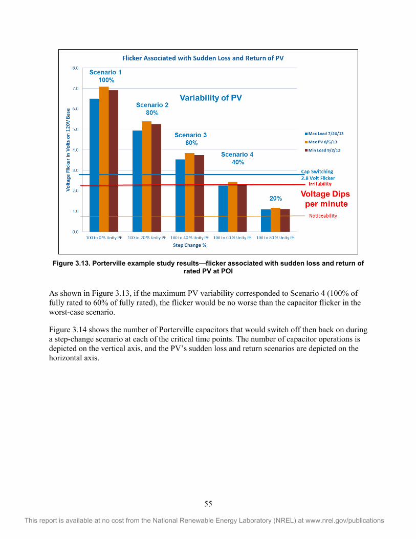
55
This report is available at no cost from the National Renewable Energy Laboratory (NREL) at www.nrel.gov/publications
Figure 3.13. Porterville example study results—flicker associated with sudden loss and return of
rated PV at POI
As shown in Figure 3.13, if the maximum PV variability corresponded to Scenario 4 (100% of fully rated to 60% of fully rated), the flicker would be no worse than the capacitor flicker in the worst-case scenario.
Figure 3.14 shows the number of Porterville capacitors that would switch off then back on during a step-change scenario at each of the critical time points. The number of capacitor operations is depicted on the vertical axis, and the PV’s sudden loss and return scenarios are depicted on the horizontal axis.
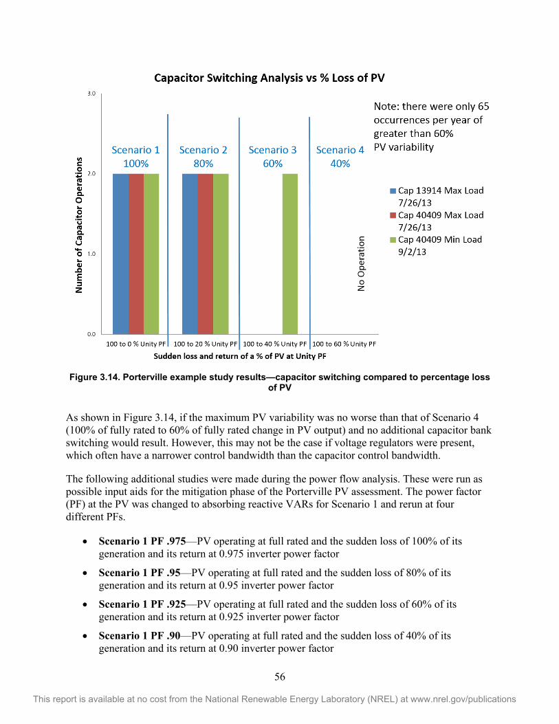
56
This report is available at no cost from the National Renewable Energy Laboratory (NREL) at www.nrel.gov/publications
Figure 3.14. Porterville example study results—capacitor switching compared to percentage loss
of PV
As shown in Figure 3.14, if the maximum PV variability was no worse than that of Scenario 4 (100% of fully rated to 60% of fully rated change in PV output) and no additional capacitor bank switching would result. However, this may not be the case if voltage regulators were present, which often have a narrower control bandwidth than the capacitor control bandwidth.
The following additional studies were made during the power flow analysis. These were run as possible input aids for the mitigation phase of the Porterville PV assessment. The power factor (PF) at the PV was changed to absorbing reactive VARs for Scenario 1 and rerun at four different PFs.
Scenario 1 PF .975—PV operating at full rated and the sudden loss of 100% of its generation and its return at 0.975 inverter power factor
Scenario 1 PF .95—PV operating at full rated and the sudden loss of 80% of its generation and its return at 0.95 inverter power factor
Scenario 1 PF .925—PV operating at full rated and the sudden loss of 60% of its generation and its return at 0.925 inverter power factor
Scenario 1 PF .90—PV operating at full rated and the sudden loss of 40% of its generation and its return at 0.90 inverter power factor
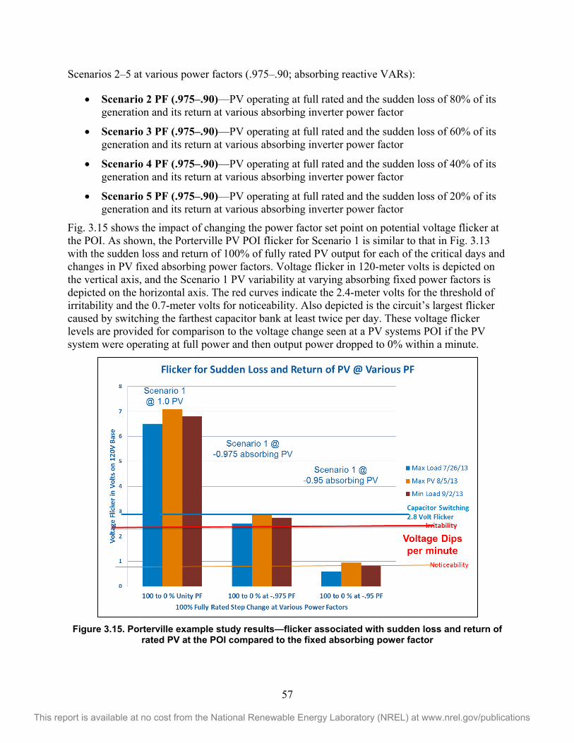
57
This report is available at no cost from the National Renewable Energy Laboratory (NREL) at www.nrel.gov/publications
Scenarios 2–5 at various power factors (.975–.90; absorbing reactive VARs):
Scenario 2 PF (.975–.90)—PV operating at full rated and the sudden loss of 80% of its generation and its return at various absorbing inverter power factor
Scenario 3 PF (.975–.90)—PV operating at full rated and the sudden loss of 60% of its generation and its return at various absorbing inverter power factor
Scenario 4 PF (.975–.90)—PV operating at full rated and the sudden loss of 40% of its generation and its return at various absorbing inverter power factor
Scenario 5 PF (.975–.90)—PV operating at full rated and the sudden loss of 20% of its generation and its return at various absorbing inverter power factor
Fig. 3.15 shows the impact of changing the power factor set point on potential voltage flicker at the POI. As shown, the Porterville PV POI flicker for Scenario 1 is similar to that in Fig. 3.13 with the sudden loss and return of 100% of fully rated PV output for each of the critical days and changes in PV fixed absorbing power factors. Voltage flicker in 120-meter volts is depicted on the vertical axis, and the Scenario 1 PV variability at varying absorbing fixed power factors is depicted on the horizontal axis. The red curves indicate the 2.4-meter volts for the threshold of irritability and the 0.7-meter volts for noticeability. Also depicted is the circuit’s largest flicker caused by switching the farthest capacitor bank at least twice per day. These voltage flicker levels are provided for comparison to the voltage change seen at a PV systems POI if the PV system were operating at full power and then output power dropped to 0% within a minute.
Figure 3.15. Porterville example study results—flicker associated with sudden loss and return of
rated PV at the POI compared to the fixed absorbing power factor
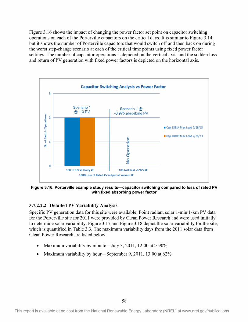
58
This report is available at no cost from the National Renewable Energy Laboratory (NREL) at www.nrel.gov/publications
Figure 3.16 shows the impact of changing the power factor set point on capacitor switching operations on each of the Porterville capacitors on the critical days. It is similar to Figure 3.14, but it shows the number of Porterville capacitors that would switch off and then back on during the worst step-change scenario at each of the critical time points using fixed power factor settings. The number of capacitor operations is depicted on the vertical axis, and the sudden loss and return of PV generation with fixed power factors is depicted on the horizontal axis.
Figure 3.16. Porterville example study results—capacitor switching compared to loss of rated PV
with fixed absorbing power factor
3.7.2.2.2 Detailed PV Variability Analysis Specific PV generation data for this site were available. Point radiant solar 1-min 1-km PV data for the Porterville site for 2011 were provided by Clean Power Research and were used initially to determine solar variability. Figure 3.17 and Figure 3.18 depict the solar variability for the site, which is quantified in Table 3.3. The maximum variability days from the 2011 solar data from Clean Power Research are listed below.
Maximum variability by minute—July 3, 2011, 12:00 at > 90%
Maximum variability by hour—September 9, 2011, 13:00 at 62%
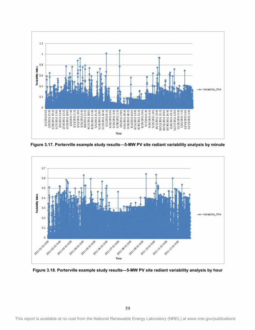
59
This report is available at no cost from the National Renewable Energy Laboratory (NREL) at www.nrel.gov/publications
Figure 3.17. Porterville example study results—5-MW PV site radiant variability analysis by minute
Figure 3.18. Porterville example study results—5-MW PV site radiant variability analysis by hour
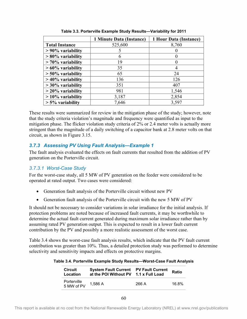
60
This report is available at no cost from the National Renewable Energy Laboratory (NREL) at www.nrel.gov/publications
Table 3.3. Porterville Example Study Results—Variability for 2011
1 Minute Data (Instance) 1 Hour Data (Instance) Total Instance 525,600 8,760 > 90% variability 5 0 > 80% variability 6 0 > 70% variability 19 0 > 60% variability 35 4 > 50% variability 65 24 > 40% variability 136 126 > 30% variability 351 407 > 20% variability 981 1,546 > 10% variability 3,187 2,854 > 5% variability 7,646 3,597
These results were summarized for review in the mitigation phase of the study; however, note that the study criteria violation’s magnitude and frequency were quantified as input to the mitigation phase. The flicker violation study criteria of 2% or 2.4 meter volts is actually more stringent than the magnitude of a daily switching of a capacitor bank at 2.8 meter volts on that circuit, as shown in Figure 3.15.
3.7.3 Assessing PV Using Fault Analysis—Example 1 The fault analysis evaluated the effects on fault currents that resulted from the addition of PV generation on the Porterville circuit.
3.7.3.1 Worst-Case Study For the worst-case study, all 5 MW of PV generation on the feeder were considered to be operated at rated output. Two cases were considered:
Generation fault analysis of the Porterville circuit without new PV
Generation fault analysis of the Porterville circuit with the new 5 MW of PV
It should not be necessary to consider variations in solar irradiance for the initial analysis. If protection problems are noted because of increased fault currents, it may be worthwhile to determine the actual fault current generated during maximum solar irradiance rather than by assuming rated PV generation output. This is expected to result in a lower fault current contribution by the PV and possibly a more realistic assessment of the worst case.
Table 3.4 shows the worst-case fault analysis results, which indicate that the PV fault current contribution was greater than 10%. Thus, a detailed protection study was performed to determine selectivity and sensitivity impacts and effects on protective margins.
Table 3.4. Porterville Example Study Results—Worst-Case Fault Analysis
Circuit Location
System Fault Current at the POI Without PV
PV Fault Current 1.1 x Full Load Ratio
Porterville 5 MW of PV 1,586 A 266 A 16.8%
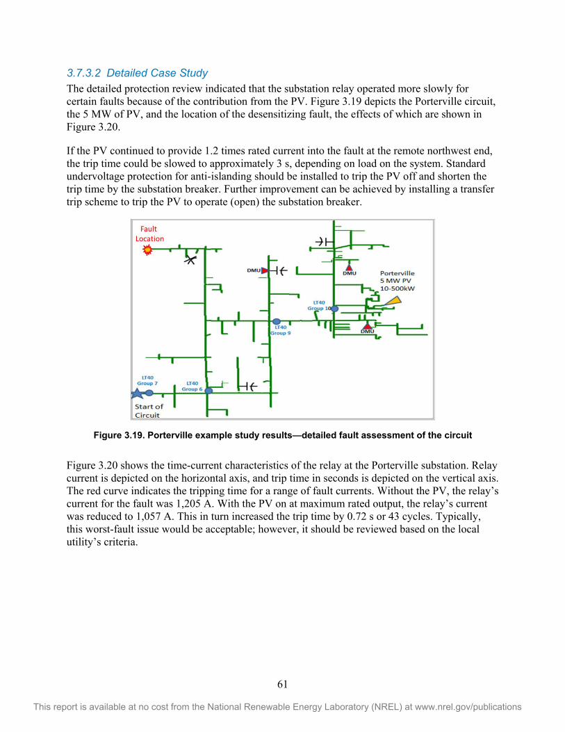
61
This report is available at no cost from the National Renewable Energy Laboratory (NREL) at www.nrel.gov/publications
3.7.3.2 Detailed Case Study The detailed protection review indicated that the substation relay operated more slowly for certain faults because of the contribution from the PV. Figure 3.19 depicts the Porterville circuit, the 5 MW of PV, and the location of the desensitizing fault, the effects of which are shown in Figure 3.20.
If the PV continued to provide 1.2 times rated current into the fault at the remote northwest end, the trip time could be slowed to approximately 3 s, depending on load on the system. Standard undervoltage protection for anti-islanding should be installed to trip the PV off and shorten the trip time by the substation breaker. Further improvement can be achieved by installing a transfer trip scheme to trip the PV to operate (open) the substation breaker.
Figure 3.19. Porterville example study results—detailed fault assessment of the circuit
Figure 3.20 shows the time-current characteristics of the relay at the Porterville substation. Relay current is depicted on the horizontal axis, and trip time in seconds is depicted on the vertical axis. The red curve indicates the tripping time for a range of fault currents. Without the PV, the relay’s current for the fault was 1,205 A. With the PV on at maximum rated output, the relay’s current was reduced to 1,057 A. This in turn increased the trip time by 0.72 s or 43 cycles. Typically, this worst-fault issue would be acceptable; however, it should be reviewed based on the local utility’s criteria.
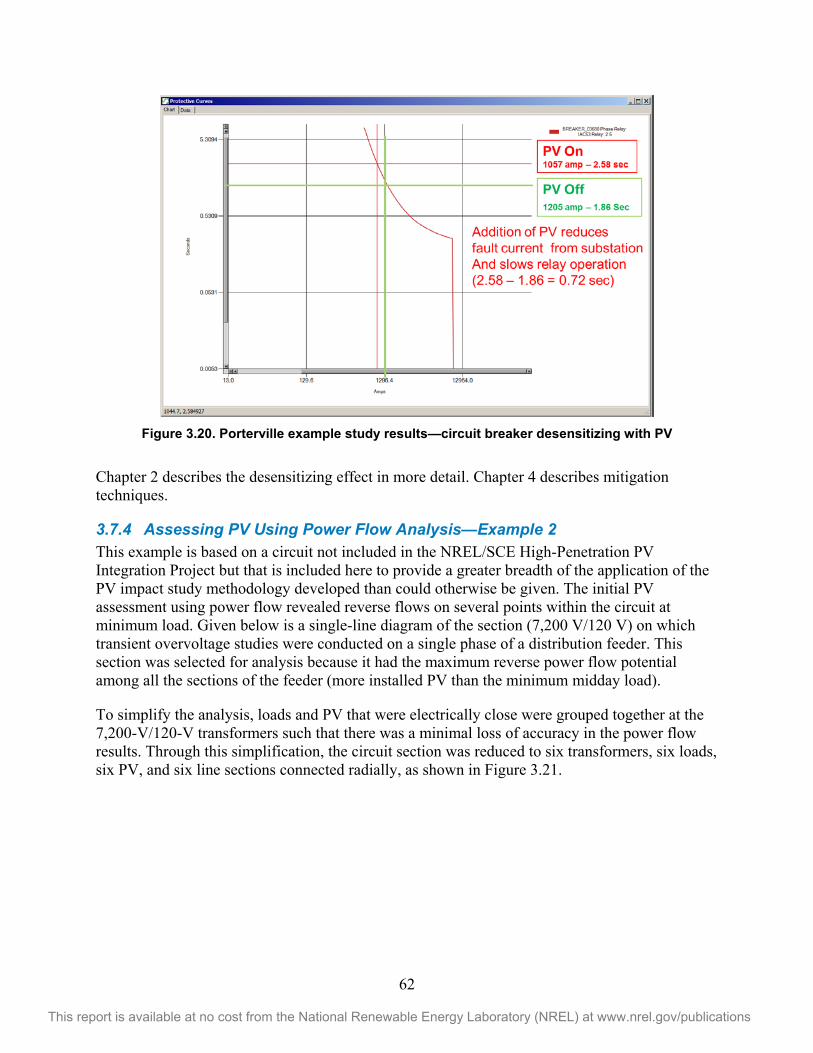
62
This report is available at no cost from the National Renewable Energy Laboratory (NREL) at www.nrel.gov/publications
Figure 3.20. Porterville example study results—circuit breaker desensitizing with PV
Chapter 2 describes the desensitizing effect in more detail. Chapter 4 describes mitigation techniques.
3.7.4 Assessing PV Using Power Flow Analysis—Example 2 This example is based on a circuit not included in the NREL/SCE High-Penetration PV Integration Project but that is included here to provide a greater breadth of the application of the PV impact study methodology developed than could otherwise be given. The initial PV assessment using power flow revealed reverse flows on several points within the circuit at minimum load. Given below is a single-line diagram of the section (7,200 V/120 V) on which transient overvoltage studies were conducted on a single phase of a distribution feeder. This section was selected for analysis because it had the maximum reverse power flow potential among all the sections of the feeder (more installed PV than the minimum midday load).
To simplify the analysis, loads and PV that were electrically close were grouped together at the 7,200-V/120-V transformers such that there was a minimal loss of accuracy in the power flow results. Through this simplification, the circuit section was reduced to six transformers, six loads, six PV, and six line sections connected radially, as shown in Figure 3.21.
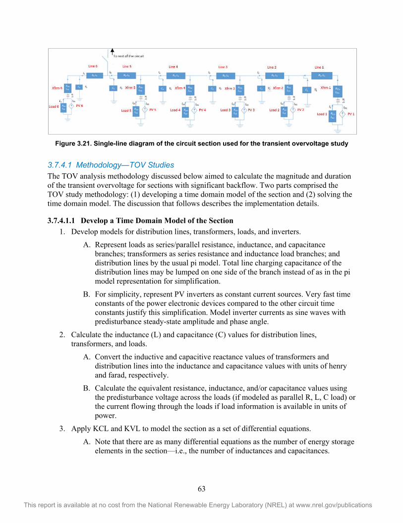
63
This report is available at no cost from the National Renewable Energy Laboratory (NREL) at www.nrel.gov/publications
Figure 3.21. Single-line diagram of the circuit section used for the transient overvoltage study
3.7.4.1 Methodology—TOV Studies The TOV analysis methodology discussed below aimed to calculate the magnitude and duration of the transient overvoltage for sections with significant backflow. Two parts comprised the TOV study methodology: (1) developing a time domain model of the section and (2) solving the time domain model. The discussion that follows describes the implementation details.
3.7.4.1.1 Develop a Time Domain Model of the Section 1. Develop models for distribution lines, transformers, loads, and inverters.
A. Represent loads as series/parallel resistance, inductance, and capacitance branches; transformers as series resistance and inductance load branches; and distribution lines by the usual pi model. Total line charging capacitance of the distribution lines may be lumped on one side of the branch instead of as in the pi model representation for simplification.
B. For simplicity, represent PV inverters as constant current sources. Very fast time constants of the power electronic devices compared to the other circuit time constants justify this simplification. Model inverter currents as sine waves with predisturbance steady-state amplitude and phase angle.
2. Calculate the inductance (L) and capacitance (C) values for distribution lines, transformers, and loads.
A. Convert the inductive and capacitive reactance values of transformers and distribution lines into the inductance and capacitance values with units of henry and farad, respectively.
B. Calculate the equivalent resistance, inductance, and/or capacitance values using the predisturbance voltage across the loads (if modeled as parallel R, L, C load) or the current flowing through the loads if load information is available in units of power.
3. Apply KCL and KVL to model the section as a set of differential equations.
A. Note that there are as many differential equations as the number of energy storage elements in the section—i.e., the number of inductances and capacitances.
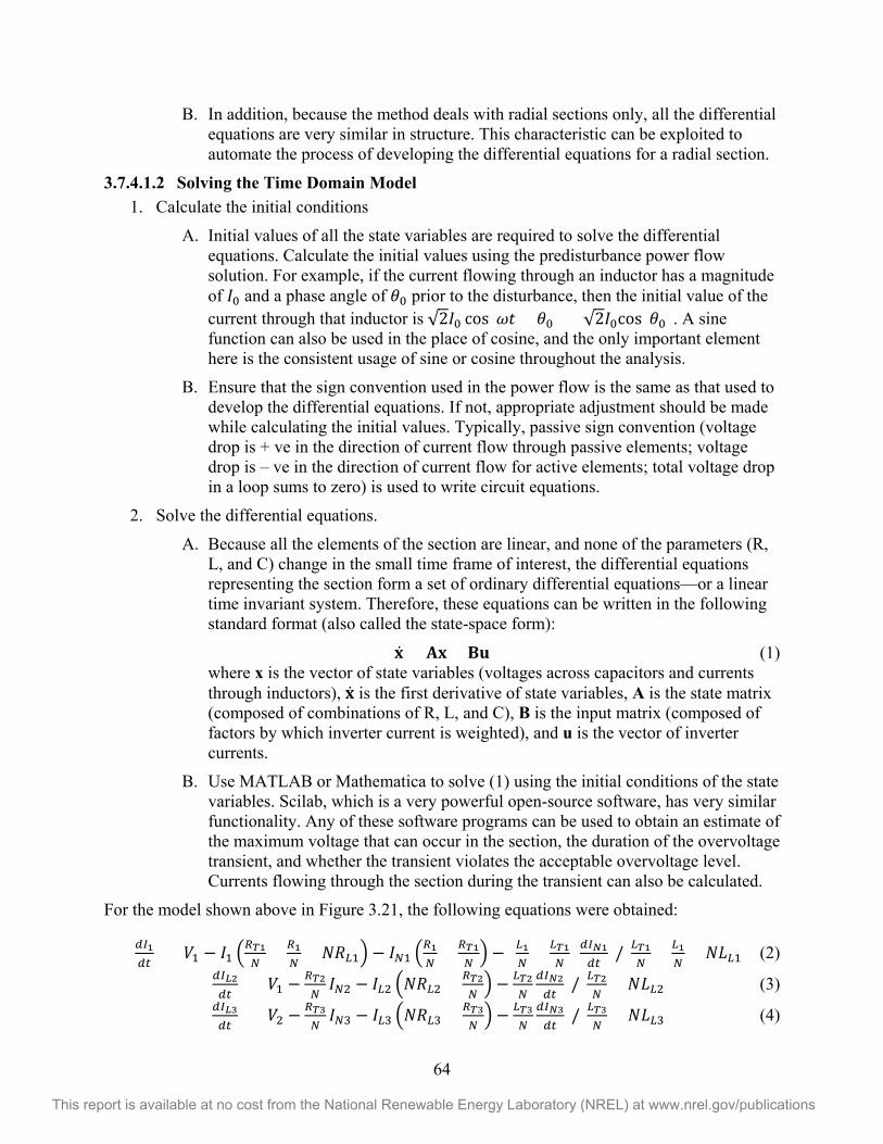
64
This report is available at no cost from the National Renewable Energy Laboratory (NREL) at www.nrel.gov/publications
B. In addition, because the method deals with radial sections only, all the differential equations are very similar in structure. This characteristic can be exploited to automate the process of developing the differential equations for a radial section.
3.7.4.1.2 Solving the Time Domain Model 1. Calculate the initial conditions
A. Initial values of all the state variables are required to solve the differential equations. Calculate the initial values using the predisturbance power flow solution. For example, if the current flowing through an inductor has a magnitude of and a phase angle of prior to the disturbance, then the initial value of the current through that inductor is 2 cos( + ) = 2 cos ( ). A sine function can also be used in the place of cosine, and the only important element here is the consistent usage of sine or cosine throughout the analysis.
B. Ensure that the sign convention used in the power flow is the same as that used to develop the differential equations. If not, appropriate adjustment should be made while calculating the initial values. Typically, passive sign convention (voltage drop is + ve in the direction of current flow through passive elements; voltage drop is – ve in the direction of current flow for active elements; total voltage drop in a loop sums to zero) is used to write circuit equations.
2. Solve the differential equations.
A. Because all the elements of the section are linear, and none of the parameters (R, L, and C) change in the small time frame of interest, the differential equations representing the section form a set of ordinary differential equations—or a linear time invariant system. Therefore, these equations can be written in the following standard format (also called the state-space form):
= + (1) where x is the vector of state variables (voltages across capacitors and currents through inductors), is the first derivative of state variables, A is the state matrix (composed of combinations of R, L, and C), B is the input matrix (composed of factors by which inverter current is weighted), and u is the vector of inverter currents.
B. Use MATLAB or Mathematica to solve (1) using the initial conditions of the state variables. Scilab, which is a very powerful open-source software, has very similar functionality. Any of these software programs can be used to obtain an estimate of the maximum voltage that can occur in the section, the duration of the overvoltage transient, and whether the transient violates the acceptable overvoltage level. Currents flowing through the section during the transient can also be calculated.
For the model shown above in Figure 3.21, the following equations were obtained:
= ( + + + ( + ) )/( + + ) (2)
= ( + )/( + ) (3)
= ( + )/( + ) (4)
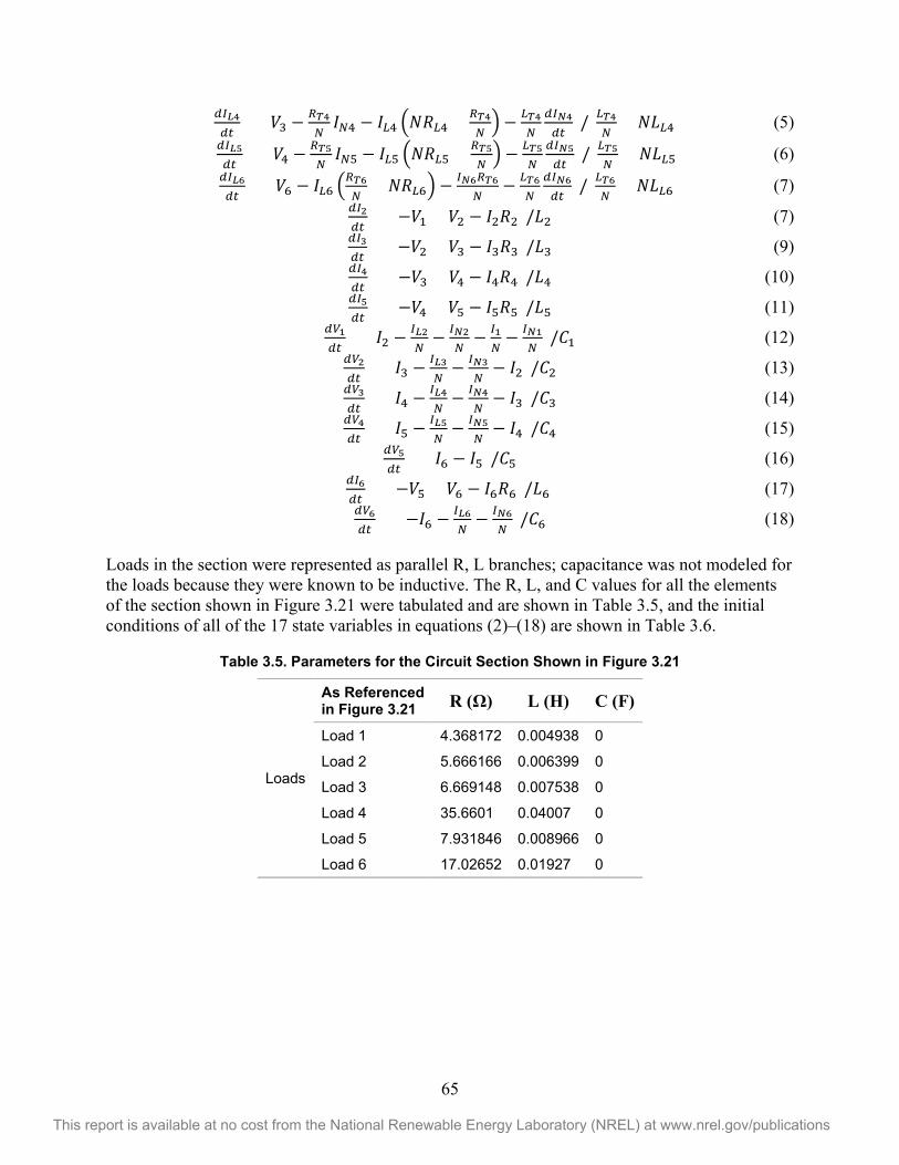
65
This report is available at no cost from the National Renewable Energy Laboratory (NREL) at www.nrel.gov/publications
= ( + )/( + ) (5)
= ( + )/( + ) (6)
= ( + )/( + ) (7)
= ( + )/ (7)
= ( + )/ (9)
= ( + )/ (10)
= ( + )/ (11)
= ( )/ (12)
= ( )/ (13)
= ( )/ (14)
= ( )/ (15)
= ( )/ (16)
= ( + )/ (17)
= ( )/ (18) Loads in the section were represented as parallel R, L branches; capacitance was not modeled for the loads because they were known to be inductive. The R, L, and C values for all the elements of the section shown in Figure 3.21 were tabulated and are shown in Table 3.5, and the initial conditions of all of the 17 state variables in equations (2)–(18) are shown in Table 3.6.
Table 3.5. Parameters for the Circuit Section Shown in Figure 3.21
Loads
As Referenced in Figure 3.21 R ( ) L (H) C (F)
Load 1 4.368172 0.004938 0
Load 2 5.666166 0.006399 0
Load 3 6.669148 0.007538 0
Load 4 35.6601 0.04007 0
Load 5 7.931846 0.008966 0
Load 6 17.02652 0.01927 0
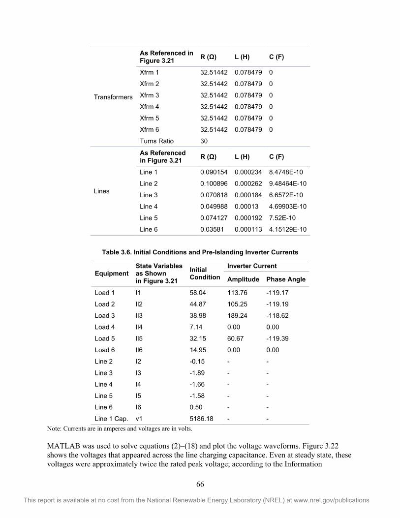
66
This report is available at no cost from the National Renewable Energy Laboratory (NREL) at www.nrel.gov/publications
Transformers
As Referenced in Figure 3.21 R ( ) L (H) C (F)
Xfrm 1 32.51442 0.078479 0
Xfrm 2 32.51442 0.078479 0
Xfrm 3 32.51442 0.078479 0
Xfrm 4 32.51442 0.078479 0
Xfrm 5 32.51442 0.078479 0
Xfrm 6 32.51442 0.078479 0
Turns Ratio 30
Lines
As Referenced in Figure 3.21 R ( ) L (H) C (F)
Line 1 0.090154 0.000234 8.4748E-10
Line 2 0.100896 0.000262 9.48464E-10
Line 3 0.070818 0.000184 6.6572E-10
Line 4 0.049988 0.00013 4.69903E-10
Line 5 0.074127 0.000192 7.52E-10
Line 6 0.03581 0.000113 4.15129E-10
Table 3.6. Initial Conditions and Pre-Islanding Inverter Currents
Equipment State Variables as Shown in Figure 3.21
Initial Condition
Inverter Current
Amplitude Phase Angle
Load 1 I1 58.04 113.76 -119.17
Load 2 Il2 44.87 105.25 -119.19
Load 3 Il3 38.98 189.24 -118.62
Load 4 Il4 7.14 0.00 0.00
Load 5 Il5 32.15 60.67 -119.39
Load 6 Il6 14.95 0.00 0.00
Line 2 I2 -0.15 - -
Line 3 I3 -1.89 - -
Line 4 I4 -1.66 - -
Line 5 I5 -1.58 - -
Line 6 I6 0.50 - -
Line 1 Cap. v1 5186.18 - - Note: Currents are in amperes and voltages are in volts. MATLAB was used to solve equations (2)–(18) and plot the voltage waveforms. Figure 3.22 shows the voltages that appeared across the line charging capacitance. Even at steady state, these voltages were approximately twice the rated peak voltage; according to the Information
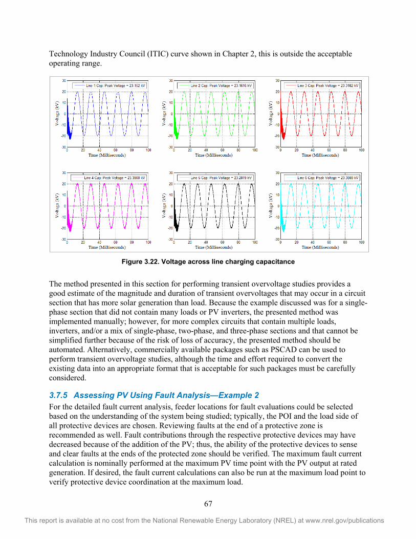
67
This report is available at no cost from the National Renewable Energy Laboratory (NREL) at www.nrel.gov/publications
Technology Industry Council (ITIC) curve shown in Chapter 2, this is outside the acceptable operating range.
Figure 3.22. Voltage across line charging capacitance
The method presented in this section for performing transient overvoltage studies provides a good estimate of the magnitude and duration of transient overvoltages that may occur in a circuit section that has more solar generation than load. Because the example discussed was for a single-phase section that did not contain many loads or PV inverters, the presented method was implemented manually; however, for more complex circuits that contain multiple loads, inverters, and/or a mix of single-phase, two-phase, and three-phase sections and that cannot be simplified further because of the risk of loss of accuracy, the presented method should be automated. Alternatively, commercially available packages such as PSCAD can be used to perform transient overvoltage studies, although the time and effort required to convert the existing data into an appropriate format that is acceptable for such packages must be carefully considered.
3.7.5 Assessing PV Using Fault Analysis—Example 2 For the detailed fault current analysis, feeder locations for fault evaluations could be selected based on the understanding of the system being studied; typically, the POI and the load side of all protective devices are chosen. Reviewing faults at the end of a protective zone is recommended as well. Fault contributions through the respective protective devices may have decreased because of the addition of the PV; thus, the ability of the protective devices to sense and clear faults at the ends of the protected zone should be verified. The maximum fault current calculation is nominally performed at the maximum PV time point with the PV output at rated generation. If desired, the fault current calculations can also be run at the maximum load point to verify protective device coordination at the maximum load.
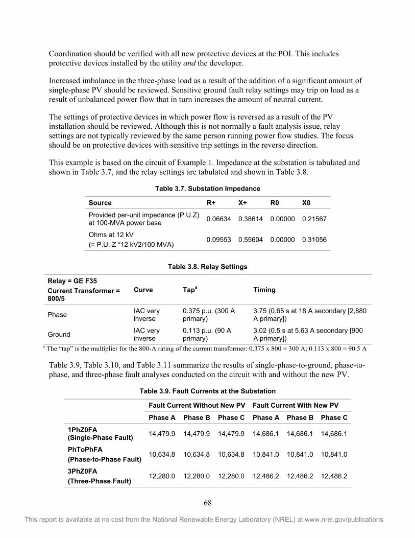
68
This report is available at no cost from the National Renewable Energy Laboratory (NREL) at www.nrel.gov/publications
Coordination should be verified with all new protective devices at the POI. This includes protective devices installed by the utility and the developer.
Increased imbalance in the three-phase load as a result of the addition of a significant amount of single-phase PV should be reviewed. Sensitive ground fault relay settings may trip on load as a result of unbalanced power flow that in turn increases the amount of neutral current.
The settings of protective devices in which power flow is reversed as a result of the PV installation should be reviewed. Although this is not normally a fault analysis issue, relay settings are not typically reviewed by the same person running power flow studies. The focus should be on protective devices with sensitive trip settings in the reverse direction.
This example is based on the circuit of Example 1. Impedance at the substation is tabulated and shown in Table 3.7, and the relay settings are tabulated and shown in Table 3.8.
Table 3.7. Substation Impedance
Source R+ X+ R0 X0
Provided per-unit impedance (P.U.Z) at 100-MVA power base 0.06634 0.38614 0.00000 0.21567
Ohms at 12 kV (= P.U. Z *12 kV2/100 MVA)
0.09553 0.55604 0.00000 0.31056
Table 3.8. Relay Settings
Relay = GE F35 Current Transformer = 800/5
Curve Tapa Timing
Phase IAC very inverse
0.375 p.u. (300 A primary)
3.75 (0.65 s at 18 A secondary [2,880 A primary])
Ground IAC very inverse
0.113 p.u. (90 A primary)
3.02 (0.5 s at 5.63 A secondary [900 A primary])
a The “tap” is the multiplier for the 800-A rating of the current transformer: 0.375 x 800 = 300 A; 0.113 x 800 = 90.5 A Table 3.9, Table 3.10, and Table 3.11 summarize the results of single-phase-to-ground, phase-to-phase, and three-phase fault analyses conducted on the circuit with and without the new PV.
Table 3.9. Fault Currents at the Substation
Fault Current Without New PV Fault Current With New PV
Phase A Phase B Phase C Phase A Phase B Phase C
1PhZ0FA (Single-Phase Fault) 14,479.9 14,479.9 14,479.9 14,686.1 14,686.1 14,686.1
PhToPhFA (Phase-to-Phase Fault)
10,634.8 10,634.8 10,634.8 10,841.0 10,841.0 10,841.0
3PhZ0FA (Three-Phase Fault)
12,280.0 12,280.0 12,280.0 12,486.2 12,486.2 12,486.2
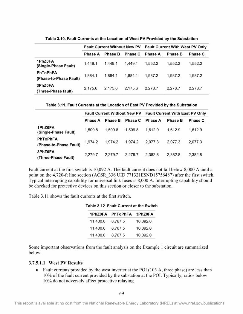
69
This report is available at no cost from the National Renewable Energy Laboratory (NREL) at www.nrel.gov/publications
Table 3.10. Fault Currents at the Location of West PV Provided by the Substation
Fault Current Without New PV Fault Current With West PV Only
Phase A Phase B Phase C Phase A Phase B Phase C
1PhZ0FA (Single-Phase Fault) 1,449.1 1,449.1 1,449.1 1,552.2 1,552.2 1,552.2
PhToPhFA (Phase-to-Phase Fault)
1,884.1 1,884.1 1,884.1 1,987.2 1,987.2 1,987.2
3PhZ0FA (Three-Phase fault)
2,175.6 2,175.6 2,175.6 2,278.7 2,278.7 2,278.7
Table 3.11. Fault Currents at the Location of East PV Provided by the Substation
Fault Current Without New PV Fault Current With East PV Only
Phase A Phase B Phase C Phase A Phase B Phase C
1PhZ0FA (Single-Phase Fault) 1,509.8 1,509.8 1,509.8 1,612.9 1,612.9 1,612.9
PhToPhFA (Phase-to-Phase Fault)
1,974.2 1,974.2 1,974.2 2,077.3 2,077.3 2,077.3
3PhZ0FA (Three-Phase Fault)
2,279.7 2,279.7 2,279.7 2,382.8 2,382.8 2,382.8
Fault current at the first switch is 10,092 A. The fault current does not fall below 8,000 A until a point on the 4,720-ft line section (ACSR_336 UID 771321E$ND15756487) after the first switch. Typical interrupting capability for universal link fuses is 8,000 A. Interrupting capability should be checked for protective devices on this section or closer to the substation.
Table 3.11 shows the fault currents at the first switch.
Table 3.12. Fault Current at the Switch
1PhZ0FA PhToPhFA 3PhZ0FA
11,400.0 8,767.5 10,092.0
11,400.0 8,767.5 10,092.0
11,400.0 8,767.5 10,092.0
Some important observations from the fault analysis on the Example 1 circuit are summarized below.
3.7.5.1.1 West PV Results Fault currents provided by the west inverter at the POI (103 A, three phase) are less than
10% of the fault current provided by the substation at the POI. Typically, ratios below 10% do not adversely affect protective relaying.
70
This report is available at no cost from the National Renewable Energy Laboratory (NREL) at www.nrel.gov/publications
For some laterals, the operation of the substation breaker will be slower because of the infeed current supplied by the inverter. For a three-phase fault at the end of the lateral farthest east, contribution from the west PV will increase the trip time slightly from 1.57 s to 1.73 s. This is because of the smaller contribution (981 A compared to 1,043 A) from the substation. Some improved protection can be provided by additional sectionalizing fuses. For example, a sectionalizing fuse or recloser should be considered for the lateral that extends to the farthest point east on the circuit.
3.7.5.1.2 East PV Results Fault currents provided by the PV at the POI (103 A, three-phase) are less than 10% of
the fault current provided by the substation at the POI. Typically, ratios below 10% do not adversely affect protective relaying.
Similar to the west PV, for some laterals, the operation of the substation breaker will be slower because of the infeed current supplied by the inverter. Some improved protection can be provided by additional sectionalizing fuses. For example, a sectionalizing fuse or recloser should be considered for the lateral that extends to the farthest point east on the circuit.
71
This report is available at no cost from the National Renewable Energy Laboratory (NREL) at www.nrel.gov/publications
4 Mitigation Techniques for High-Penetration PV Impacts
4.1 Introduction A utility is responsible to all the customers on a distribution circuit and prefers that the addition of any load or generation not result in power quality issues for adjacent customers. The interconnection of a PV system can be related to the interconnection of a large motor load. In this case, the customer with the large motor load and its starting disturbance is typically responsible for not bothering adjacent customers. The connection, start-up, and operation of this large motor can be simulated, and the interconnection can be facilitated with a number of very well-known and accepted techniques that are usually the burden of the motor owner. Consider the process of motor start-up and operation similar to that of PV variability.
An advanced PV inverter, at near-zero marginal cost, could have the ability to virtually eliminate voltage variation on a distribution feeder resulting from variations in the real power output of a PV plant. A PV inverter could even mitigate the effects of load-induced voltage variations elsewhere on the feeder. An advanced PV inverter could also mitigate the effects of its own variable real power output on the grid voltage by correcting changes while they are happening and maintaining dynamic VAR reserve in a similar way as is done in modern transmission-system VAR compensators.
A utility may also be able to modify its system to accommodate the PV without causing detrimental effects to existing customers. Mitigation measures for the utility to consider include requiring a separate feeder, requiring transfer trip, reconfiguring circuitry including phase balancing, and revising existing equipment and its operation (e.g., by revising settings for capacitor and regulator controls, implementing relay settings, adding new components, and reconductoring and/or extending lines).
Some mitigation methods may require actions only at the PV system, some may require actions only by the utility, and some may require a combination of both to allow for the connection of a PV system. The discussion that follows presents a number of techniques to mitigate the adverse impacts of PV.
4.2 Mitigation Techniques Supported by PV Inverter Capabilities Two sets of PV inverter capabilities are described below. In all, the focus is primarily on coordinating reactive output to variations in real output and the corresponding voltage effects. The first is constant power factor, which is perhaps the simplest means of mitigation at the PV. The second is a list of advanced capabilities typically available in modern PV inverters.
4.2.1 Constant Power Factor Operation This method of mitigating the impact of PV requires changing the power factor set point, and hence the reactive power output, of an inverter to address the voltage criteria violations. This is perhaps the simplest method to mitigate voltage-related impacts by using PV inverters.
Injecting real power (watts) or reactive power (VAR) will increase the voltage at the point of injection; conversely, absorbing real power or reactive power will decrease the voltage. By
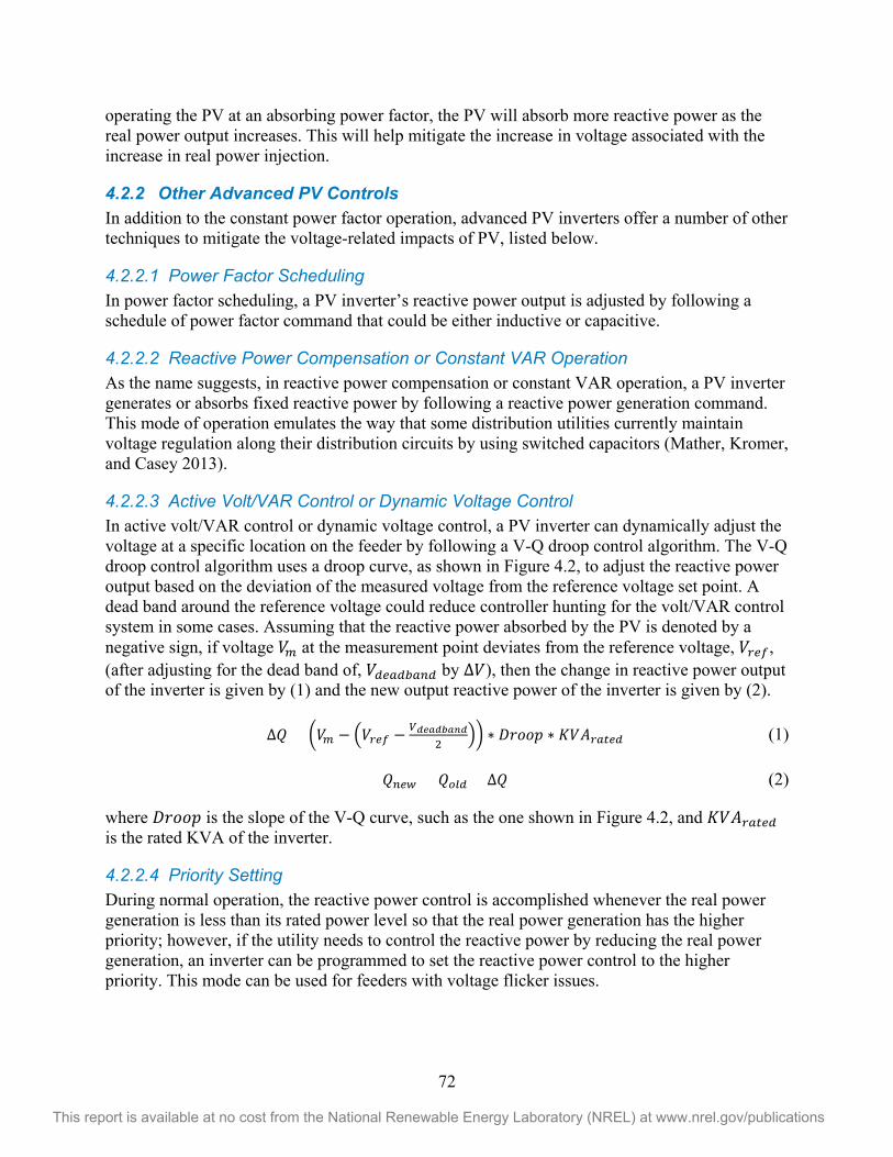
72
This report is available at no cost from the National Renewable Energy Laboratory (NREL) at www.nrel.gov/publications
operating the PV at an absorbing power factor, the PV will absorb more reactive power as the real power output increases. This will help mitigate the increase in voltage associated with the increase in real power injection.
4.2.2 Other Advanced PV Controls In addition to the constant power factor operation, advanced PV inverters offer a number of other techniques to mitigate the voltage-related impacts of PV, listed below.
4.2.2.1 Power Factor Scheduling In power factor scheduling, a PV inverter’s reactive power output is adjusted by following a schedule of power factor command that could be either inductive or capacitive.
4.2.2.2 Reactive Power Compensation or Constant VAR Operation As the name suggests, in reactive power compensation or constant VAR operation, a PV inverter generates or absorbs fixed reactive power by following a reactive power generation command. This mode of operation emulates the way that some distribution utilities currently maintain voltage regulation along their distribution circuits by using switched capacitors (Mather, Kromer, and Casey 2013).
4.2.2.3 Active Volt/VAR Control or Dynamic Voltage Control In active volt/VAR control or dynamic voltage control, a PV inverter can dynamically adjust the voltage at a specific location on the feeder by following a V-Q droop control algorithm. The V-Q droop control algorithm uses a droop curve, as shown in Figure 4.2, to adjust the reactive power output based on the deviation of the measured voltage from the reference voltage set point. A dead band around the reference voltage could reduce controller hunting for the volt/VAR control system in some cases. Assuming that the reactive power absorbed by the PV is denoted by a negative sign, if voltage at the measurement point deviates from the reference voltage, , (after adjusting for the dead band of, by ), then the change in reactive power output of the inverter is given by (1) and the new output reactive power of the inverter is given by (2).
= (1)
= + (2)
where is the slope of the V-Q curve, such as the one shown in Figure 4.2, and is the rated KVA of the inverter.
4.2.2.4 Priority Setting During normal operation, the reactive power control is accomplished whenever the real power generation is less than its rated power level so that the real power generation has the higher priority; however, if the utility needs to control the reactive power by reducing the real power generation, an inverter can be programmed to set the reactive power control to the higher priority. This mode can be used for feeders with voltage flicker issues.
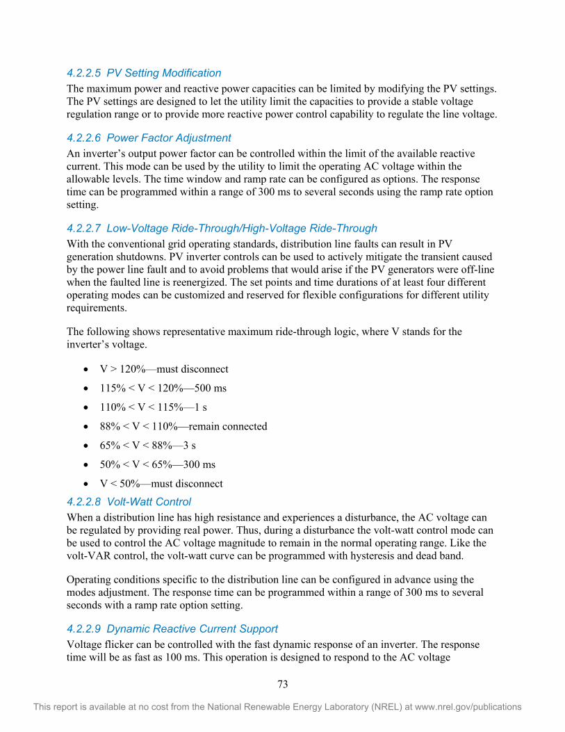
73
This report is available at no cost from the National Renewable Energy Laboratory (NREL) at www.nrel.gov/publications
4.2.2.5 PV Setting Modification The maximum power and reactive power capacities can be limited by modifying the PV settings. The PV settings are designed to let the utility limit the capacities to provide a stable voltage regulation range or to provide more reactive power control capability to regulate the line voltage.
4.2.2.6 Power Factor Adjustment An inverter’s output power factor can be controlled within the limit of the available reactive current. This mode can be used by the utility to limit the operating AC voltage within the allowable levels. The time window and ramp rate can be configured as options. The response time can be programmed within a range of 300 ms to several seconds using the ramp rate option setting.
4.2.2.7 Low-Voltage Ride-Through/High-Voltage Ride-Through With the conventional grid operating standards, distribution line faults can result in PV generation shutdowns. PV inverter controls can be used to actively mitigate the transient caused by the power line fault and to avoid problems that would arise if the PV generators were off-line when the faulted line is reenergized. The set points and time durations of at least four different operating modes can be customized and reserved for flexible configurations for different utility requirements.
The following shows representative maximum ride-through logic, where V stands for the inverter’s voltage.
V > 120%—must disconnect
115% < V < 120%—500 ms
110% < V < 115%—1 s
88% < V < 110%—remain connected
65% < V < 88%—3 s
50% < V < 65%—300 ms
V < 50%—must disconnect
4.2.2.8 Volt-Watt Control When a distribution line has high resistance and experiences a disturbance, the AC voltage can be regulated by providing real power. Thus, during a disturbance the volt-watt control mode can be used to control the AC voltage magnitude to remain in the normal operating range. Like the volt-VAR control, the volt-watt curve can be programmed with hysteresis and dead band.
Operating conditions specific to the distribution line can be configured in advance using the modes adjustment. The response time can be programmed within a range of 300 ms to several seconds with a ramp rate option setting.
4.2.2.9 Dynamic Reactive Current Support Voltage flicker can be controlled with the fast dynamic response of an inverter. The response time will be as fast as 100 ms. This operation is designed to respond to the AC voltage
74
This report is available at no cost from the National Renewable Energy Laboratory (NREL) at www.nrel.gov/publications
fluctuation for the short duration caused by load changes or line disturbances. The dynamic reactive current support curve can be programmed with optional hysteresis and dead band. This mode can be operated in conjunction with the priority setting to regulate AC voltage.
4.2.2.10 Intelligent Volt-VAR Control The distribution line voltage can be regulated linearly within an inverter’s available power capacity. The AC voltage control can be coordinated in the SCADA level with other control equipment, such as capacitor banks or voltage regulators. The volt-VAR curve can be programmed with optional hysteresis and dead band. Operating conditions specific to the distribution line can be configured in advance using the modes adjustment. The response time can be programmed to between 300 ms and several seconds using the ramp rate option setting.
4.3 Mitigation Techniques to Alleviate PV Impacts 4.3.1 Steady-State Voltage Impacts 4.3.1.1 High-Voltage Impacts Pockets of high voltage can occur on the distribution circuit during low-load conditions, particularly in places that have a large single PV or a cluster of PV systems. Voltages should stay below the permissible high-voltage thresholds, otherwise they can reduce the life of electrical equipment and cause PV inverters to trip off-line.
Mitigation measures include running the PV at an absorbing power factor, which may negate needs for circuit reactive compensation. Use of line-drop compensation can be considered if the flow through is not masked. Modifying switch capacitor bank controls is another method that can be used to resolve high-voltage issues. Consider removing fixed bank capacitors or converting them to switched capacitors.
4.3.1.2 Low-Voltage Impacts Pockets of low voltage can occur in the distribution circuit, particularly during peak loads when the PV output may be masking the real native load of the circuit for which the voltage regulation has been designed.
Perhaps the best mitigation for voltage regulation issues is to operate the PV at a leading power factor (absorbing VARs from the system). Utility mitigations for these same issues include improving or narrowing the circuit voltage regulation. This may be accomplished by modifying the control settings of the capacitors, LTCs, and voltage regulators and/or by installing new regulation equipment.
When voltage drop compensation is used and is fooled by the masked PV output downstream of the native load, one mitigation technique is to reset the voltage drop compensation to reflect the masked PV output. Another solution is to install additional voltage regulation equipment, which would negate the need for compensation.
4.3.1.3 Flicker Impacts Variations in PV output can cause fluctuations in customer service voltage. These voltage fluctuations can cause flicker, which may be irritating to customers and may also result in malfunctioning appliances. The size of PV that can be connected to a point on a feeder without
75
This report is available at no cost from the National Renewable Energy Laboratory (NREL) at www.nrel.gov/publications
causing unacceptable voltage fluctuations is limited. Solar PV impact studies should assess the potential of voltage flicker that can be caused by high penetrations of solar PV. Because the power output of solar PV can fluctuate considerably and much faster than the response of traditional voltage regulation equipment, there is potential for voltage flicker when large amounts of solar PV are connected. High or low voltages may occur because of the fluctuations in PV output and before the regulation has a chance to move. In addition, capacitors may switch excessively with high PV, further exacerbating high- and low-voltage conditions as well as increasing the operations of these devices. Mitigation measures include running the PV at absorbing power factors. The utility should review the phase balance of the circuitry. A more phase-balanced circuit will generally offer some relief.
4.3.1.4 Active Device Movement Impacts In addition to the flicker problems previously discussed, PV variability can cause voltage excursions on the feeder that lead to the hunting of tap changers, voltage regulators, and switched capacitor banks. These conditions may not result in voltages outside ANSI voltage limits, but they can result in many more operations of the active devices thus requiring increased maintenance and/or replacement.
The best way to handle these excessive motion problems, short of limiting the size of the PV system, may be to modify the PV power factor setting. If setting a non-unity power factor is not possible or does not resolve the issue, the utility may be able to modify the active device controls. For LTCs and voltage regulators, changing the set point voltage, bandwidth, and or time delays may be a viable option. For switched capacitor banks, changing the type of control and its time delays may also be a viable method.
Note that LTCs and capacitor banks may be gang controlled by a single phase. Review the selected phase to ensure that the circuit is phase balanced and that the controlled phase is chosen.
4.3.2 Dynamic Voltage Impacts 4.3.2.1 TOV Impacts Caused By Islanding TOV caused by load rejection can occur at a sectionalizing device when that device is being back-fed and a fault occurs. This TOV can damage sensitive and utility equipment, such as lightning arresters. The ability to sense an overvoltage and then trip the unit in as short as 10 cycles (as required by IEEE 1547) is no guarantee that the overvoltage will not cause damage. TOV has been primarily associated with induction and synchronous rotating generators. Fortunately, PV inverters are much less likely to experience these conditions, which are primarily associated with rotating power generation equipment; however, high-penetration PV TOV is a new area of investigation.
Mitigating TOV can be accomplished by modifying an inverter’s protection system (e.g., anti-islanding or reverse power relays in less than 10 cycles). On the utility side, phase balancing should be considered as a mitigation strategy for single-phase reverse flows. For three-phase reverse flows, consider moving the protective device if no substantial adverse reliability affects are expected. Note that this may be a short-term means of resolving the issue.
Mitigation may also be accomplished using lightning arrestors. Surge arrestors, which can absorb the energy generated because of the longer duration of the TOV, can help mitigate the TOV. It is
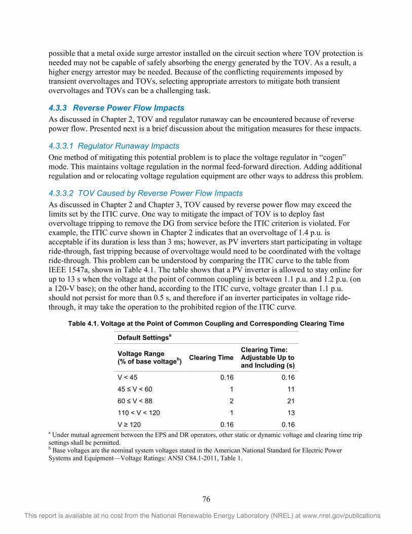
76
This report is available at no cost from the National Renewable Energy Laboratory (NREL) at www.nrel.gov/publications
possible that a metal oxide surge arrestor installed on the circuit section where TOV protection is needed may not be capable of safely absorbing the energy generated by the TOV. As a result, a higher energy arrestor may be needed. Because of the conflicting requirements imposed by transient overvoltages and TOVs, selecting appropriate arrestors to mitigate both transient overvoltages and TOVs can be a challenging task.
4.3.3 Reverse Power Flow Impacts As discussed in Chapter 2, TOV and regulator runaway can be encountered because of reverse power flow. Presented next is a brief discussion about the mitigation measures for these impacts.
4.3.3.1 Regulator Runaway Impacts One method of mitigating this potential problem is to place the voltage regulator in “cogen” mode. This maintains voltage regulation in the normal feed-forward direction. Adding additional regulation and or relocating voltage regulation equipment are other ways to address this problem.
4.3.3.2 TOV Caused by Reverse Power Flow Impacts As discussed in Chapter 2 and Chapter 3, TOV caused by reverse power flow may exceed the limits set by the ITIC curve. One way to mitigate the impact of TOV is to deploy fast overvoltage tripping to remove the DG from service before the ITIC criterion is violated. For example, the ITIC curve shown in Chapter 2 indicates that an overvoltage of 1.4 p.u. is acceptable if its duration is less than 3 ms; however, as PV inverters start participating in voltage ride-through, fast tripping because of overvoltage would need to be coordinated with the voltage ride-through. This problem can be understood by comparing the ITIC curve to the table from IEEE 1547a, shown in Table 4.1. The table shows that a PV inverter is allowed to stay online for up to 13 s when the voltage at the point of common coupling is between 1.1 p.u. and 1.2 p.u. (on a 120-V base); on the other hand, according to the ITIC curve, voltage greater than 1.1 p.u. should not persist for more than 0.5 s, and therefore if an inverter participates in voltage ride-through, it may take the operation to the prohibited region of the ITIC curve.
Table 4.1. Voltage at the Point of Common Coupling and Corresponding Clearing Time
Default Settingsa
Voltage Range (% of base voltageb) Clearing Time
Clearing Time: Adjustable Up to and Including (s)
V < 45 0.16 0.16
1 11
2 21
110 < V < 120 1 13
0.16 0.16 a Under mutual agreement between the EPS and DR operators, other static or dynamic voltage and clearing time trip settings shall be permitted. b Base voltages are the nominal system voltages stated in the American National Standard for Electric Power Systems and Equipment—Voltage Ratings: ANSI C84.1-2011, Table 1.
77
This report is available at no cost from the National Renewable Energy Laboratory (NREL) at www.nrel.gov/publications
Using sacrificial arrestors is another option to mitigate the TOV; however, these may be difficult to coordinate with utility arrestors and could also result in problems of coordination with load withstand ratings (Walling 2014).
4.3.4 Overload Impacts A simple example of this problem has surfaced for high penetrations of net-metering customer PV additions under the same transformer. There may be some instances when a minimum customer load coincides with high PV generation, such as during a midweek summer holiday. The mitigation for this potential problem is to replace the distribution transformer with one that can carry the entire PV output while the customer load is near zero.
4.3.5 System Protection Impacts Methods of mitigating system protection impacts are highly dependent on the specific impact in question. Refer to Chapter 2, Chapter 3, and Appendix B for more specific details.
Mitigation techniques for system protection impacts are included below. Note that common impacts are listed, but it is not possible to include solutions for all problems.
A solution to almost all impacts unacceptable to a utility is to deny connection of the PV or restrict output during certain conditions, such as circuit reconfiguration. This solution is noted here and not in the individual cases below. In some cases, major system rebuilding can mitigate the impact. Major rebuilds such as installing a line extension, dedicated feeder, or substation are also not included in the individual cases below.
4.3.5.1 Exceeding the Interrupting Rating Impacts As described in Chapter 2, the additional fault current from the added PV may cause the interrupting rating of protective devices to be exceeded. This impact is similar to the increase in fault current resulting from a transformer change or circuit reconfiguration. When this occurs, modifications are required. Typically, the interrupting device needs to be replaced with equipment with an adequate rating. Installing back-up series current-limiting fuses upstream may be an economical solution for fuses.
Although it may reduce reliability, removing underrated equipment or using jumpers may be a temporary solution if the upstream protective devices provide adequate fault sensing.
4.3.5.2 Desensitizing Substation Relay Impacts As described in Chapter 2, when fault current from PV combines with substation fault current on a branch, the fault current is effectively reduced from the substation breaker. This will slow the operating time of the breaker and possibly reduce the contribution from the breaker to an unacceptably low level. Several solutions are possible:
Consider adding a set of fuses if the branch is not protected by a sectionalizing fuse.
Accept sequential tripping. The PV should trip off-line at some point, and the substation current will increase. Consider decreasing the trip time for undervoltage to assist in speeding up the clearing time of the substation breaker.
78
This report is available at no cost from the National Renewable Energy Laboratory (NREL) at www.nrel.gov/publications
Lower the pickup value or time dial of the substation relay if loadability and selectivity considerations permit.
4.3.5.3 Inselectivity Caused By Increased Fault Current Impacts As described in Chapter 2, increased fault current may cause overcurrent protective devices to become inselective. For example, a higher fault current level may cause the total clearing time for a downstream fuse to exceed or approach the minimum melt time of the upstream fuse.
A comparison of operating characteristics in a selectivity study is required to determine the best solution. Replacing the upstream or downstream fuse with a device with different time-current characteristics may be the best solution. In some cases, a fuse may be removed. Also consider replacing sectionalizing fuses with sectionalizers if an upstream recloser is involved.
If no reasonable solution is found and the inselectivity remains, operating personnel should be alerted by notes on the operating map and other related documents used in the control room by field personnel.
4.3.5.4 Isolating PV for an Upstream Fault Impacts As described in Chapter 2, the fault contribution from the PV may cause an upstream protective device to operate for faults upstream of that device. This is unlikely if the protective device is capable of carrying the full output of the PV, because the fault contribution is typically approximately 1.1 times the full output current of the PV.
Note that this isolation is extremely undesirable if it will interrupt other customers downstream of the protective device. If studies show this possibility, shortening the trip time for low-voltage or directional overcurrent relaying may mitigate the problem by stopping the PV fault current contribution before the upstream device trips. Also consider increasing the trip value or trip time for the upstream protective device.
4.3.5.5 Line-to-Ground Overvoltage Impacts As described in Chapter 2, if the PV is connected via a delta-wye transformer, ground faults upstream of the PV may result in high voltage on the unfaulted phases.
The PV needs to be shut down quickly for line-to-ground overvoltage. Potential sensing devices are required on the high-voltage side of the transformer. An N59 relay connected across the “broken” delta of the sensing circuit, as shown in Figure 2.12, will sense the overvoltage. A coordination study should be performed to determine the overvoltage and trip time settings. An overly sensitive setting that trips in a few cycles may operate for ground faults distant from the PV.
Also consider using a grounded wye-wye transformer instead of a delta-wye transformer. The grounded wye on the high-voltage side will help stabilize voltages on the unfaulted phases.
4.3.5.6 Nuisance Fuse Blowing Impacts As noted in Chapter 2, fault contribution from PV systems may cause a fuse to blow that would have otherwise remained intact. As shown in Figure 2.13, during a temporary fault beyond the
79
This report is available at no cost from the National Renewable Energy Laboratory (NREL) at www.nrel.gov/publications
50-k fuse, the recloser operates on a fast curve, which is intended to clear the fault before the 50-k fuse blows. If fault current continues to flow from the PV, the fuse may blow.
Consider decreasing the trip time for undervoltage to limit the length of time of the PV fault contribution. Also, a directional overcurrent relay could be used to trip the PV for fault contributions at or above the current that will blow the fuse.
If fuse saving by the fast operation of reclosers is not a critical reliability issue, then consider allowing the fuse to clear the fault. These should be noted on the related operating maps and other documents to alert operating personnel.
4.3.5.7 Reclosing Out of Synchronism Impacts As noted in Chapter 2, if automatic reclosing times are too fast, the PV may still be online and have lost synchronism with the utility system. If the device closes out of synchronism, this is considered a fault condition and may cause the breaker to trip or cause equipment damage. The reclosing time should be long enough to permit the PV system to detect the condition and go off-line. If the possibility of an out-of-synchronism closing still remains, consider installing voltage-sensing devices on the PV side of the recloser or breaker and then installing synch-check relaying—or permit closing only if the PV side of the recloser is de-energized.
4.3.5.8 Islanding Impacts As noted in Chapter 2, if a breaker or other switchable device is opened with PV downstream, there is a possibility of islanding the PV with other customer load.
Various protective measures are used to prevent these unintentional islands. PV is often equipped with island detection systems (anti-islanding systems) that can sense the absence of the utility. Many types of anti-islanding systems exist. If a PV system is compliant with IEEE 1547 and UL 1741, its islanding detection capability has been tested. Refer to IEEE 1547 and UL 1741 for more details about island detection requirements.
Although the requirements for detection of an island are detailed in IEEE 1547 and UL 1741, the specific mechanisms and methods for detecting an island are not. Thus, anti-islanding schemes for different inverters may vary, and the details of these schemes are often proprietary. Therefore, as penetrations of PV increase, some concern exists because of the potential for interaction among different anti-islanding schemes. Additionally, advanced inverter functionality such as low-voltage ride-through may increase the likelihood of an unintentional island forming, because in those cases low voltage can no longer be used for islanding detection.
If anti-islanding protection is either not available or is insufficient, direct transfer trip (DTT) may be utilized. DTT is often expensive as protection-grade communication channels are typically required, especially if reclosers between the breaker and PV must be included in the scheme. Permissive transfer trip has been proposed as a lower-cost alternative—for example, the loss of a “heartbeat” signal from the substation for approximately 2 s would cause the PV to trip.
Typically, other than the communications-based measures mentioned above, mitigation of unintentional islanding concerns at PV levels approaching expected load levels include some form of laboratory testing to show that the PV inverter’s algorithms are capable of detection the
80
This report is available at no cost from the National Renewable Energy Laboratory (NREL) at www.nrel.gov/publications
formation of an island. The specific methods used to detect an islanded condition may be chosen and/or the specific algorithm settings (gains, set points, time delays) may be adjusted to insure IEEE 1547 compliance.
4.3.5.9 Miscounting Sectionalizer Impacts As noted in Chapter 2, sectionalizers that require the fault current to fall to a relatively low value (e.g., below 1 A) to count current pulses before opening may miscount because of current provided from the PV. This condition is similar to nuisance fuse blowing, and the mitigation technique is similar. Consider decreasing the trip time for undervoltage to limit the length of time of the PV fault contribution. Also, a directional overcurrent relay could be used to trip the PV for fault contributions at or above the current that will cause the sectionalizer to miscount.
4.3.5.10 Reverse Power Relay Operation on Secondary Network Impacts As noted in Chapter 2, during normal (unfaulted) operation, network protectors typically open for reverse power and may operate for excessive PV connected to the secondary network. The amount of PV should be limited to ensure that there is not excessive protector operation. An accurate model of the network system is needed to perform power flow studies that can determine the permissible amount of PV. At some point, it may be necessary to configure the PV in a spot network or to some other point on the system.
4.3.5.11 Reverse Power Relay Operation in Substation Impacts As noted in Chapter 2, in a case with very large PV, which typically may have a dedicated feeder, the protection system would normally be set to accept reverse flow; however, if reverse flow through the substation transformer is undesirable, the transformer relay may be set to trip the dedicated feeder. Because this would be an intended operation, this possibility should be noted on operating maps and other related documents to alert operating personnel.
Refer to Chapter 2 for a description of PV impact and mitigation techniques for the following:
Cold load pickup
Faults within a PV zone
Fault causing voltage sag and tripping PV
4.4 Porterville Example—Constant Power Factor Operation As the heading suggests, this method of mitigating the impact of PV requires changing the power factor set point, and hence the reactive power output, of the inverter to address the voltage criteria violations. This is perhaps the simplest method of mitigating voltage-related impacts using PV inverters. The method for identifying the power factor that can mitigate the voltage-related impacts is presented by means of three Southern California Edison circuits: Porterville, Palmdale, and Fontana, California.
Porterville was considered in Example 1 in Chapter 3. In Chapter 3, voltage flicker was determined via a PV impact assessment study to exist on the circuit with loss and return of solar generation at 100% of rated output and unity power factor. To understand how constant power factor operation can mitigate flicker, step-change analysis similar to that used in Chapter 3 to identify voltage flicker was performed for a number of scenarios with varying percentage loss-
81
This report is available at no cost from the National Renewable Energy Laboratory (NREL) at www.nrel.gov/publications
of-generation and power factors. The scenarios studied and the observations from the analyses are discussed below.
The following additional studies were made to examine power flow. These were run as input aids for the mitigation phase of the Porterville PV assessment. Then the power factor at the PV was changed to absorbing reactive VARs for Scenario 1 and rerun at four different power factors. The scenarios are described below, and the results of the analysis are illustrated in Figure 4.1
Scenario 1 PF .975—PV operating at full rated power and the sudden loss of 100% of its generation and its return, at .975 inverter power factor
Scenario 1 PF .95—PV operating at full rated and the sudden loss of 80% of its generation and its return, at .95 inverter power factor
Scenario 1 PF .925—PV operating at full rated and the sudden loss of 60% of its generation and its return, at .925 inverter power factor
Scenario 1 PF .90—PV operating at full rated and the sudden loss of 40% of its generation and its return, at .90 inverter power factor
Scenarios 2–5 at various power factors—.975–.90; absorbing reactive VARs:
Scenarios 2 PF (.975–.90)—PV operating at full rated and the sudden loss of 80% of its generation and its return at various absorbing inverter power factor
Scenarios 3 PF (.975–.90)—PV operating at full rated and the sudden loss of 60% of its generation and its return at various absorbing inverter power factor
Scenarios 4 PF (.975–.90)—PV operating at full rated and the sudden loss of 40% of its generation and its return at various absorbing inverter power factor
Scenarios 5 PF (.975–.90)—PV operating at full rated and the sudden loss of 20% of its generation and its return at various absorbing inverter power factor
The impact of adding a new 5-MW PV plant was analyzed. Three critical days and hours were chosen as the enveloping operating conditions for the step-change analysis: maximum native load day and hour, minimum native load day and maximum PV hour, and maximum PV day and hour. Five scenarios were evaluated for each critical time point: 100%, 80%, 60%, 40%, and 20% loss and return of generation. This allowed both the potential for overvoltage and flicker because of PV variability to be evaluated simultaneously.
Adding PV resulted in a slight overvoltage when the start of circuit voltage was kept at 124 V; however, this problem was easily resolved by reducing the start of the circuit voltage to 122.5 V. A voltage flicker criterion violation was also observed at the PV point of common coupling for the scenarios with 100% loss and return of generation. This was reduced to the level observed in the circuit from the operation of existing capacitor banks by operating the inverter at a 0.975 absorbing power factor. If the flicker were to be reduced further, the power factor would need to be made even more absorbing. Figure 4.1 illustrates these results.
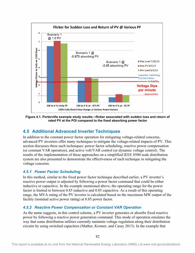
82
This report is available at no cost from the National Renewable Energy Laboratory (NREL) at www.nrel.gov/publications
Figure 4.1. Porterville example study results—flicker associated with sudden loss and return of
rated PV at the POI compared to the fixed absorbing power factor
4.5 Additional Advanced Inverter Techniques In addition to the constant power factor operation for mitigating voltage-related concerns, advanced PV inverters offer many techniques to mitigate the voltage-related impacts of PV. This section discusses three such techniques: power factor scheduling, reactive power compensation (or constant VAR operation), and active volt/VAR control (or dynamic voltage control). The results of the implementation of these approaches on a simplified IEEE 8500 node distribution system are also presented to demonstrate the effectiveness of each technique in mitigating the voltage concerns.
4.5.1 Power Factor Scheduling In this method, similar to the fixed power factor technique described earlier, a PV inverter’s reactive power output is adjusted by following a power factor command that could be either inductive or capacitive. In the example mentioned above, the operating range for the power factor is limited to between 0.85 inductive and 0.85 capacitive. As a result of this operating range, the MVA rating of the PV inverter is calculated based on the maximum MW output of the facility (nominal active power rating) at 0.85 power factor.
4.5.2 Reactive Power Compensation or Constant VAR Operation As the name suggests, in this control scheme, a PV inverter generates or absorbs fixed reactive power by following a reactive power generation command. This mode of operation emulates the way that some distribution utilities currently maintain voltage regulation along their distribution circuits by using switched capacitors (Mather, Kromer, and Casey 2013). In the example that
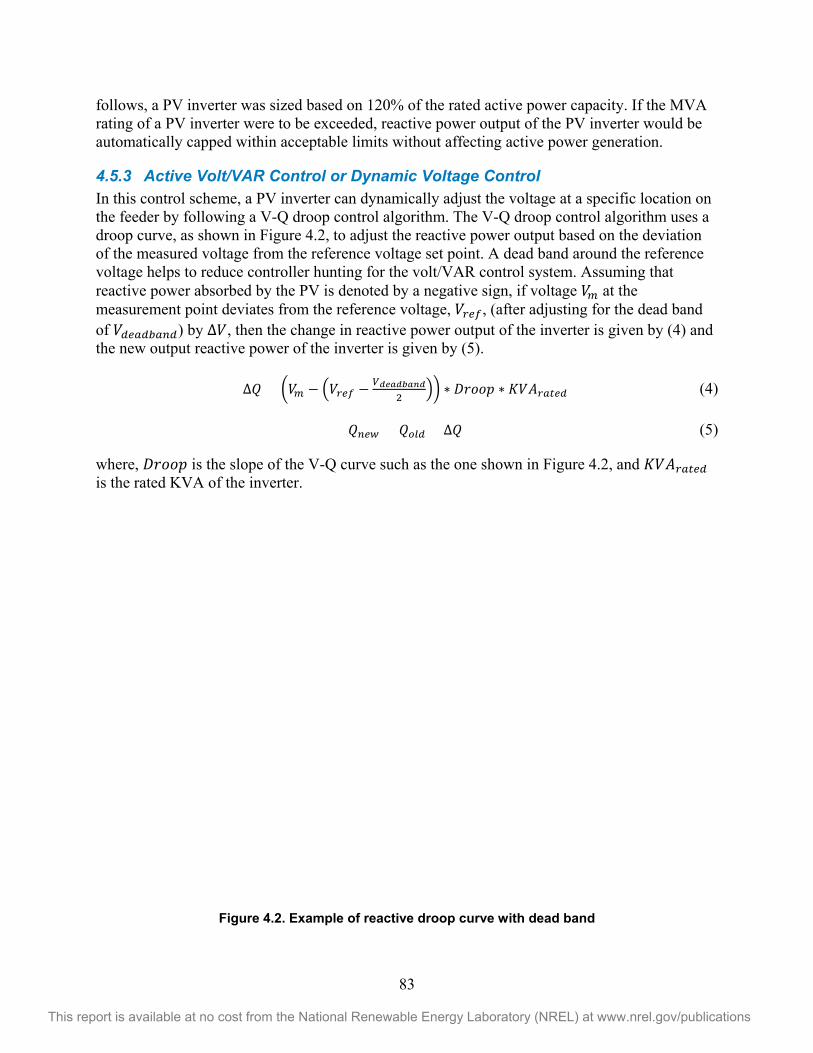
83
This report is available at no cost from the National Renewable Energy Laboratory (NREL) at www.nrel.gov/publications
follows, a PV inverter was sized based on 120% of the rated active power capacity. If the MVA rating of a PV inverter were to be exceeded, reactive power output of the PV inverter would be automatically capped within acceptable limits without affecting active power generation.
4.5.3 Active Volt/VAR Control or Dynamic Voltage Control In this control scheme, a PV inverter can dynamically adjust the voltage at a specific location on the feeder by following a V-Q droop control algorithm. The V-Q droop control algorithm uses a droop curve, as shown in Figure 4.2, to adjust the reactive power output based on the deviation of the measured voltage from the reference voltage set point. A dead band around the reference voltage helps to reduce controller hunting for the volt/VAR control system. Assuming that reactive power absorbed by the PV is denoted by a negative sign, if voltage at the measurement point deviates from the reference voltage, , (after adjusting for the dead band of ) by , then the change in reactive power output of the inverter is given by (4) and the new output reactive power of the inverter is given by (5).
= (4)
= + (5)
where, is the slope of the V-Q curve such as the one shown in Figure 4.2, and is the rated KVA of the inverter.
Figure 4.2. Example of reactive droop curve with dead band
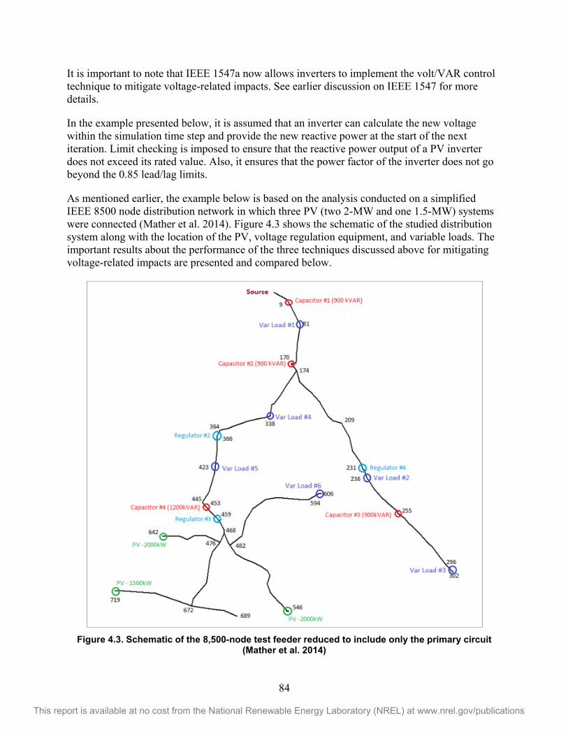
84
This report is available at no cost from the National Renewable Energy Laboratory (NREL) at www.nrel.gov/publications
It is important to note that IEEE 1547a now allows inverters to implement the volt/VAR control technique to mitigate voltage-related impacts. See earlier discussion on IEEE 1547 for more details.
In the example presented below, it is assumed that an inverter can calculate the new voltage within the simulation time step and provide the new reactive power at the start of the next iteration. Limit checking is imposed to ensure that the reactive power output of a PV inverter does not exceed its rated value. Also, it ensures that the power factor of the inverter does not go beyond the 0.85 lead/lag limits.
As mentioned earlier, the example below is based on the analysis conducted on a simplified IEEE 8500 node distribution network in which three PV (two 2-MW and one 1.5-MW) systems were connected (Mather et al. 2014). Figure 4.3 shows the schematic of the studied distribution system along with the location of the PV, voltage regulation equipment, and variable loads. The important results about the performance of the three techniques discussed above for mitigating voltage-related impacts are presented and compared below.
Figure 4.3. Schematic of the 8,500-node test feeder reduced to include only the primary circuit
(Mather et al. 2014)
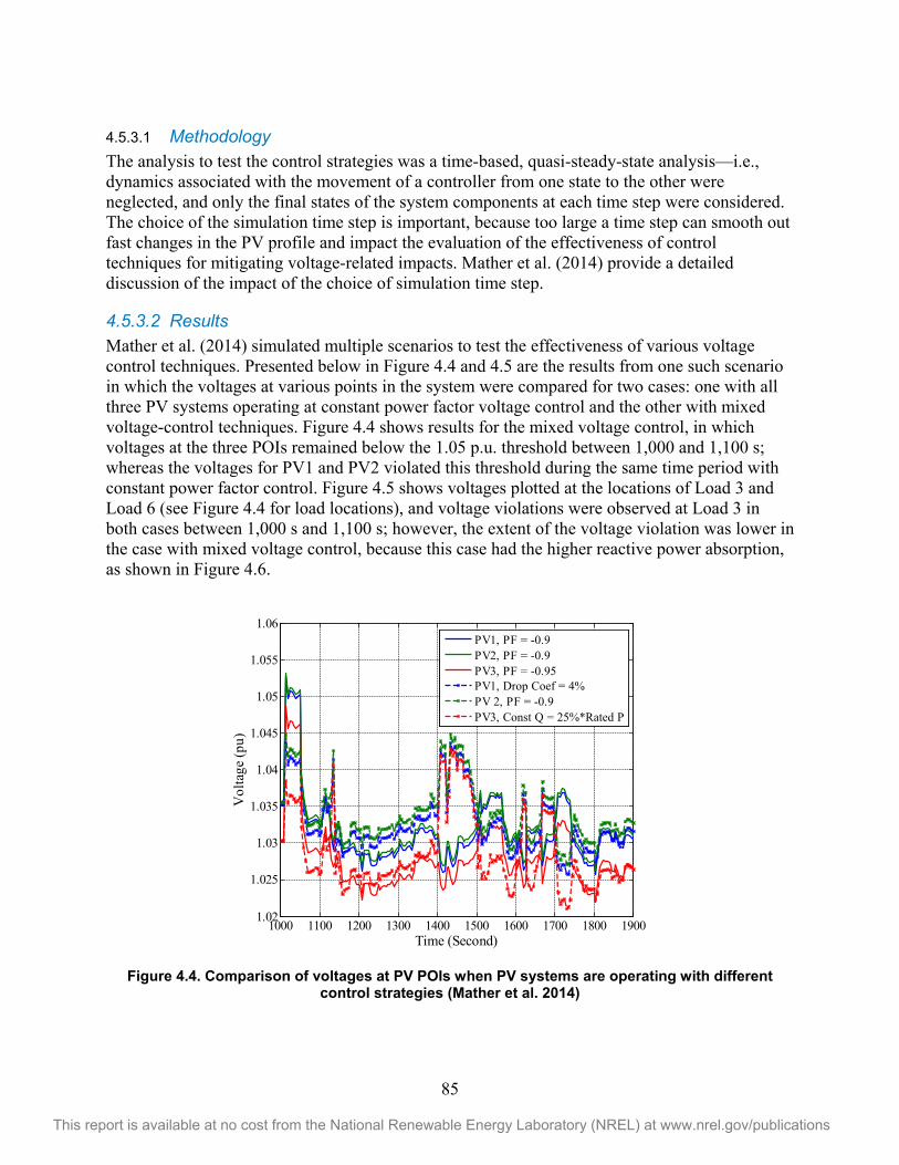
85
This report is available at no cost from the National Renewable Energy Laboratory (NREL) at www.nrel.gov/publications
4.5.3.1 Methodology
The analysis to test the control strategies was a time-based, quasi-steady-state analysis—i.e., dynamics associated with the movement of a controller from one state to the other were neglected, and only the final states of the system components at each time step were considered. The choice of the simulation time step is important, because too large a time step can smooth out fast changes in the PV profile and impact the evaluation of the effectiveness of control techniques for mitigating voltage-related impacts. Mather et al. (2014) provide a detailed discussion of the impact of the choice of simulation time step.
4.5.3.2 Results Mather et al. (2014) simulated multiple scenarios to test the effectiveness of various voltage control techniques. Presented below in Figure 4.4 and 4.5 are the results from one such scenario in which the voltages at various points in the system were compared for two cases: one with all three PV systems operating at constant power factor voltage control and the other with mixed voltage-control techniques. Figure 4.4 shows results for the mixed voltage control, in which voltages at the three POIs remained below the 1.05 p.u. threshold between 1,000 and 1,100 s; whereas the voltages for PV1 and PV2 violated this threshold during the same time period with constant power factor control. Figure 4.5 shows voltages plotted at the locations of Load 3 and Load 6 (see Figure 4.4 for load locations), and voltage violations were observed at Load 3 in both cases between 1,000 s and 1,100 s; however, the extent of the voltage violation was lower in the case with mixed voltage control, because this case had the higher reactive power absorption, as shown in Figure 4.6.
Figure 4.4. Comparison of voltages at PV POIs when PV systems are operating with different
control strategies (Mather et al. 2014)
1000 1100 1200 1300 1400 1500 1600 1700 1800 19001.02
1.025
1.03
1.035
1.04
1.045
1.05
1.055
1.06
Time (Second)
Vol
tage
(pu)
PV1, PF = -0.9PV2, PF = -0.9PV3, PF = -0.95PV1, Drop Coef = 4%PV 2, PF = -0.9PV3, Const Q = 25%*Rated P
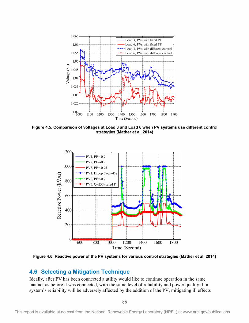
86
This report is available at no cost from the National Renewable Energy Laboratory (NREL) at www.nrel.gov/publications
Figure 4.5. Comparison of voltages at Load 3 and Load 6 when PV systems use different control
strategies (Mather et al. 2014)
Figure 4.6. Reactive power of the PV systems for various control strategies (Mather et al. 2014)
4.6 Selecting a Mitigation Technique Ideally, after PV has been connected a utility would like to continue operation in the same manner as before it was connected, with the same level of reliability and power quality. If a system’s reliability will be adversely affected by the addition of the PV, mitigating ill effects
1000 1100 1200 1300 1400 1500 1600 1700 1800 19001.02
1.025
1.03
1.035
1.04
1.045
1.05
1.055
1.06
1.065
Time (Second)
Vol
tage
(pu)
Load 3, PVs with fixed PFLoad 6, PVs with fixed PFLoad 3, PVs with different controlLoad 6, PVs with different control
600 800 1000 1200 1400 1600 18000
200
400
600
800
1000
1200
Time (Second)
Rea
ctiv
e Po
wer
(kV
Ar)
PV1, PF=-0.9PV2, PF=-0.9PV3, PF=-0.95PV1, Droop Coef=4%PV2, PF=-0.9PV3, Q=25% rated P
87
This report is available at no cost from the National Renewable Energy Laboratory (NREL) at www.nrel.gov/publications
should be the responsibility of the PV owner, and this level is the best place at which to resolve issues. This is typically done with the simplest mitigation strategies.
Mitigation techniques that have proven effective on an individual system should be used accordingly. The simplest and least expensive mitigation alternatives are typically preferred by a utility, its rate payers, and PV system owners. Modifying a PV power plant or operation is often the simplest solution. Modifying utility equipment is typically expensive and takes additional time.
88
This report is available at no cost from the National Renewable Energy Laboratory (NREL) at www.nrel.gov/publications
References Agalgaonkar, Y.P.; Pal, B.C.; Jabr, R.A., “Distribution Voltage Control Considering the Impact of PV Generation on Tap Changers and Autonomous Regulators,” IEEE Transactions on Power Systems, (29:1), January, 2014.
Durbak, D.W., “Temporary Overvoltages Following Transformer Energizing,” Power Technology, (99), Sept., 2006, accessed February 2015: http://w3.usa.siemens.com/datapool/us/SmartGrid/docs/pti/2006June/Temporary_Overvoltages_Following_Transformer_Energizing.pdf.
Ellis, A.; Nelson, R.; Von Engeln, E.; Walling, R.; McDowell, J.; Casey, L.; Seymour, E.; Peter, W.; Barker, C.; Kirby, B., Reactive Power Interconnection Requirements for PV and Wind Plants—Recommendations to NERC, SAND2012-1098. Albuquerque, NM: Sandia National Laboratories, February, 2012, accessed August 2014: http://energy.sandia.gov/wp/wp-content/gallery/uploads/Reactive-Power-Requirements-for-PV-and-Wind-SAND2012-1098.pdf.
IEEE. (2011a). 1453-2011—IEEE Recommended Practice—Adoption of IEC 61000-4-15:2010, Electromagnetic Compatibility (EMC)—Testing and Measurement Techniques—Flickermeter—Functional and Design Specifications. Piscataway, NJ.
IEEE. (2011b). C62.82.1-2010—IEEE Standard for Insulation Coordination—Definitions, Principles, and Rules. Piscataway, NJ.
IEEE. (2014). 1547a-2014—IEEE Standard for Interconnecting Distributed Resources with Electric Power Systems: Amendment 1. Approved May 16, 2014. Piscataway, NJ.
Katiraei, K.; Agüero, J.R., “Solar PV Integration Challenges,” IEEE Power and Energy Magazine, May/June, 2011.
Lawhead, L.; Horak, J.; Madani, V.; Vaziri, M., “Cold Load Pick-Up—Theory and Industry Practices,” in proc. of Georgia Tech Protective Relay Conference, May 3–5, 2006, Atlanta, GA.
Mather, B.A.; Kromer, M.A.; Casey, L., “Advanced Photovoltaic Inverter Functionality Using 500-kW Power Hardware-in-Loop Complete System Laboratory Testing,” in proc. of IEEE Innovative Smart Grid Technologies Conference, Feb. 24–27, 2013, Washington, D.C.
Mather, B.A.; Shah, S.; Norris, B.L.; Dise, J.H.; Yu, L.; Paradis, D.; Katiraei, F.; Seguin, R.; Costyk, D.; Woyak, J.; Jung, J.; Russell, K.; Broadwater, R., NREL/SCE High Penetration PV Integration Project: FY13 Annual Report, Golden, CO: National Renewable Energy Laboratory, June, 2014, accessed August 2014: http://www.nrel.gov/docs/fy14osti/61269.pdf.
McGranaghan, M. Ortmeyer, T.; Crudele, D.; Key, T.; Smith, J.; Barker, P., Renewable Systems Interconnection Study: Advanced Grid Planning and Operations, SAND2008-0944 P. Albuquerque, NM: Sandia National Laboratories, February, 2008, accessed February 2015: https://www1.eere.energy.gov/solar/pdfs/advanced_grid_planning_operations.pdf.

89
This report is available at no cost from the National Renewable Energy Laboratory (NREL) at www.nrel.gov/publications
Nelson, A., Hoke, A., Chakraborty, S., Ropp, M., Chebahtah, J., Wang, T., Zimmerly, B., Inverter Load Rejection Over-Votlage Testing,” National Renewable Energy Laboratory, February, 2015, accessed September 2015: http://www.nrel.gov/docs/fy15osti/63510.pdf
Seal, B., Common Functions for Smart Inverters. Version 3. 3002002233. Palo Alto, CA: Electric Power Research Institute, 2014.
UL. (2010). UL 1741: Standard for Inverters, Converters, Controllers and Interconnection System Equipment for Use with Distributed Energy Resources, 2010. http://ulstandards.ul.com/standard/?id=1741.
Walling, R. “Grounding and Overvoltage Requirements for Distributed Generation,” in proc. of IEEE Power and Energy Society General Meeting, National Harbor, MD, July, 2014, accessed August 2014: http://www.ieee-pes.org/presentations/td2014/td2014p-000544.pdf.
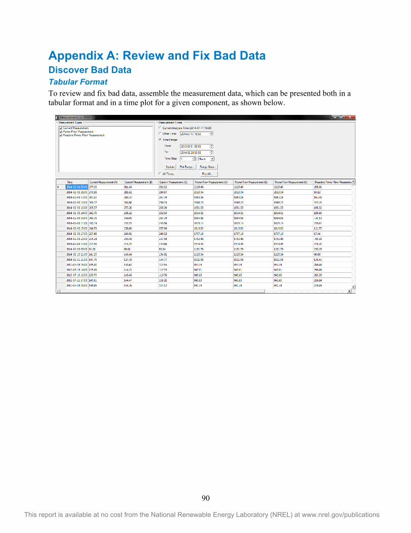
90
This report is available at no cost from the National Renewable Energy Laboratory (NREL) at www.nrel.gov/publications
Appendix A: Review and Fix Bad Data Discover Bad Data Tabular Format To review and fix bad data, assemble the measurement data, which can be presented both in a tabular format and in a time plot for a given component, as shown below.
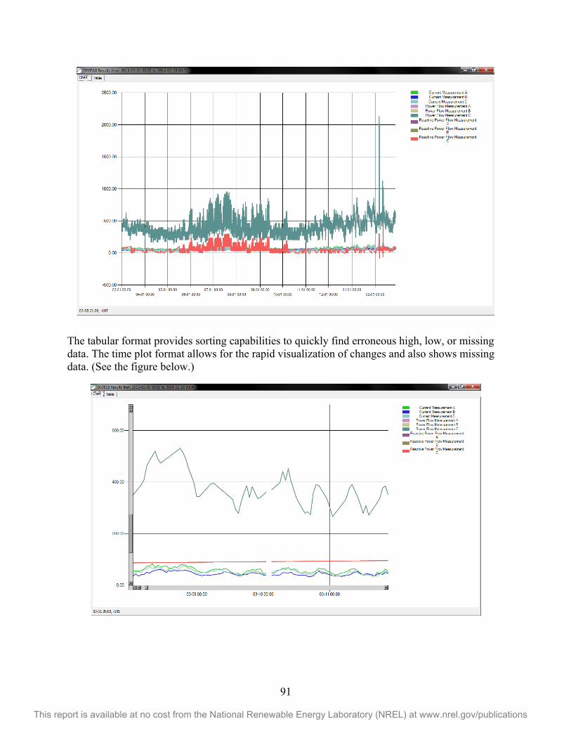
91
This report is available at no cost from the National Renewable Energy Laboratory (NREL) at www.nrel.gov/publications
The tabular format provides sorting capabilities to quickly find erroneous high, low, or missing data. The time plot format allows for the rapid visualization of changes and also shows missing data. (See the figure below.)
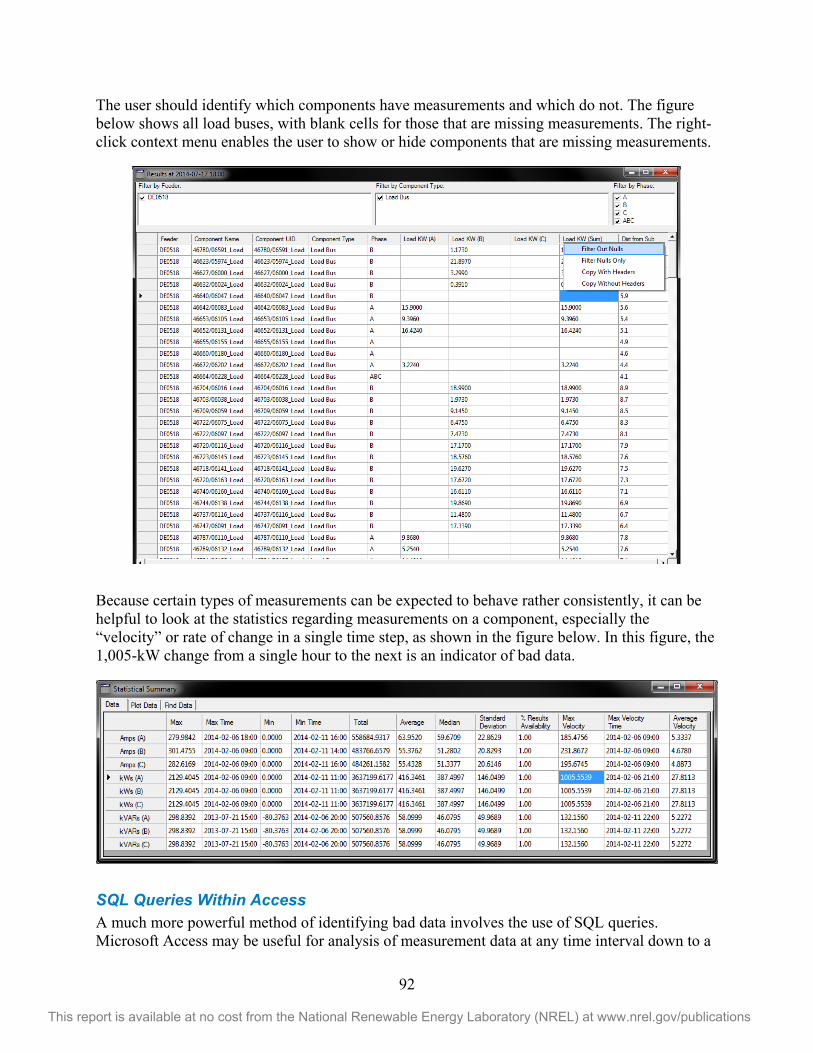
92
This report is available at no cost from the National Renewable Energy Laboratory (NREL) at www.nrel.gov/publications
The user should identify which components have measurements and which do not. The figure below shows all load buses, with blank cells for those that are missing measurements. The right-click context menu enables the user to show or hide components that are missing measurements.
Because certain types of measurements can be expected to behave rather consistently, it can be helpful to look at the statistics regarding measurements on a component, especially the “velocity” or rate of change in a single time step, as shown in the figure below. In this figure, the 1,005-kW change from a single hour to the next is an indicator of bad data.
SQL Queries Within Access A much more powerful method of identifying bad data involves the use of SQL queries. Microsoft Access may be useful for analysis of measurement data at any time interval down to a
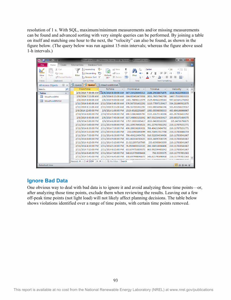
93
This report is available at no cost from the National Renewable Energy Laboratory (NREL) at www.nrel.gov/publications
resolution of 1 s. With SQL, maximum/minimum measurements and/or missing measurements can be found and advanced sorting with very simple queries can be performed. By joining a table on itself and matching one hour to the next, the “velocity” can also be found, as shown in the figure below. (The query below was run against 15-min intervals; whereas the figure above used 1-h intervals.)
Ignore Bad Data One obvious way to deal with bad data is to ignore it and avoid analyzing those time points—or, after analyzing those time points, exclude them when reviewing the results. Leaving out a few off-peak time points (not light load) will not likely affect planning decisions. The table below shows violations identified over a range of time points, with certain time points removed.
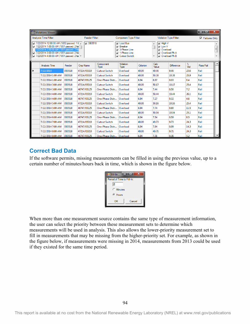
94
This report is available at no cost from the National Renewable Energy Laboratory (NREL) at www.nrel.gov/publications
Correct Bad Data If the software permits, missing measurements can be filled in using the previous value, up to a certain number of minutes/hours back in time, which is shown in the figure below.
When more than one measurement source contains the same type of measurement information, the user can select the priority between these measurement sets to determine which measurements will be used in analysis. This also allows the lower-priority measurement set to fill in measurements that may be missing from the higher-priority set. For example, as shown in the figure below, if measurements were missing in 2014, measurements from 2013 could be used if they existed for the same time period.
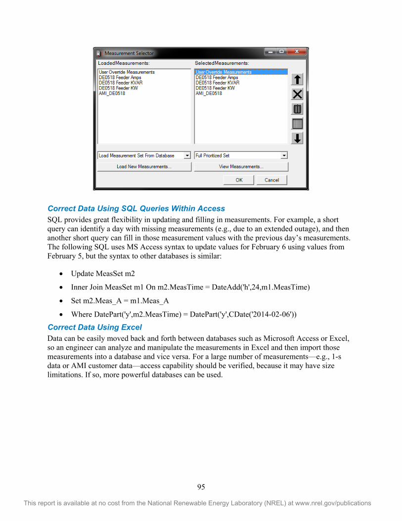
95
This report is available at no cost from the National Renewable Energy Laboratory (NREL) at www.nrel.gov/publications
Correct Data Using SQL Queries Within Access SQL provides great flexibility in updating and filling in measurements. For example, a short query can identify a day with missing measurements (e.g., due to an extended outage), and then another short query can fill in those measurement values with the previous day’s measurements. The following SQL uses MS Access syntax to update values for February 6 using values from February 5, but the syntax to other databases is similar:
Update MeasSet m2
Inner Join MeasSet m1 On m2.MeasTime = DateAdd('h',24,m1.MeasTime)
Set m2.Meas_A = m1.Meas_A
Where DatePart('y',m2.MeasTime) = DatePart('y',CDate('2014-02-06'))
Correct Data Using Excel Data can be easily moved back and forth between databases such as Microsoft Access or Excel, so an engineer can analyze and manipulate the measurements in Excel and then import those measurements into a database and vice versa. For a large number of measurements—e.g., 1-s data or AMI customer data—access capability should be verified, because it may have size limitations. If so, more powerful databases can be used.
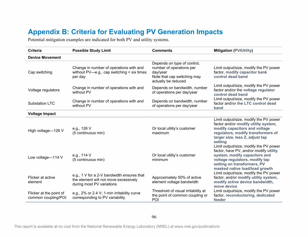
96
This report is available at no cost from the National Renewable Energy Laboratory (NREL) at www.nrel.gov/publications
Appendix B: Criteria for Evaluating PV Generation Impacts Potential mitigation examples are indicated for both PV and utility systems.
Criteria Possible Study Limit Comments Mitigation (PV/Utility)
Device Movement
Cap switching Change in number of operations with and without PV—e.g., cap switching < six times per day
Depends on type of control, number of operations per day/year Note that cap switching may actually be reduced
Limit output/size, modify the PV power factor, modify capacitor bank control dead band
Voltage regulators Change in number of operations with and without PV
Depends on bandwidth, number of operations per day/year
Limit output/size, modify the PV power factor and/or the voltage regulator control dead band
Substation LTC Change in number of operations with and without PV
Depends on bandwidth, number of operations per day/year
Limit output/size, modify the PV power factor and/or the LTC control dead band
Voltage Impact
High voltage—126 V e.g., 126 V (5 continuous min)
Or local utility’s customer maximum
Limit output/size, modify the PV power factor and/or modify utility system, modify capacitors and voltage regulators, modify transformers of larger size, less Z, adjust tap setting
Low voltage—114 V e.g., 114 V (5 continuous min)
Or local utility’s customer minimum
Limit output/size, modify the PV power factor, have PV, and/or modify utility system, modify capacitors and voltage regulators, modify tap setting on transformers, PV masked native load/load growth
Flicker at active element
e.g., 1 V for a 2-V bandwidth ensures that the element will not move excessively during most PV variations
Approximately 50% of active element voltage bandwidth
Limit output/size, modify the PV power factor, and/or modify utility system, modify active device bandwidth, move device
Flicker at the point of common coupling/POI
e.g., 2% or 2.4 V; 1-min irritability curve corresponding to PV variability
Threshold of visual irritability at the point of common coupling or POI
Limit output/size, modify the PV power factor, reconductoring, dedicated feeder
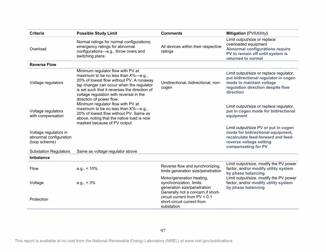
97
This report is available at no cost from the National Renewable Energy Laboratory (NREL) at www.nrel.gov/publications
Criteria Possible Study Limit Comments Mitigation (PV/Utility)
Overload
Normal ratings for normal configurations; emergency ratings for abnormal configurations—e.g., throw overs and switching plans
All devices within their respective ratings
Limit output/size or replace overloaded equipment Abnormal configurations require PV to remain off until system is returned to normal
Reverse Flow
Voltage regulators
Minimum regulator flow with PV at maximum to be no less than X%—e.g., 20% of lowest flow without PV. A runaway tap changer can occur when the regulator is set such that it reverses the direction of voltage regulation with reversal in the direction of power flow.
Unidirectional, bidirectional, non-cogen
Limit output/size or replace regulator, put bidirectional regulator in cogen mode to maintain voltage regulation direction despite flow direction
Voltage regulators with compensation
Minimum regulator flow with PV at maximum to be no less than X%—e.g., 20% of lowest flow without PV. Same as above, noting that the native load is now masked because of PV output
Limit output/size or replace regulator, put in cogen mode for bidirectional equipment
Voltage regulators in abnormal configuration (loop scheme)
Limit output/size PV or put in cogen mode for bidirectional equipment, recalculate feed-forward and feed-reverse voltage setting compensating for PV
Substation Regulators Same as voltage regulator above Imbalance
Flow e.g., < 10% Reverse flow and synchronizing, limits generation size/penetration
Limit output/size, modify the PV power factor, and/or modify utility system by phase balancing
Voltage e.g., < 3% Motor/generation heating, synchronization, limits generation size/penetration
Limit output/size, modify the PV power factor, and/or modify utility system by phase balancing
Protection
Generally not a concern if short-circuit current from PV < 0.1 short-circuit current from substation
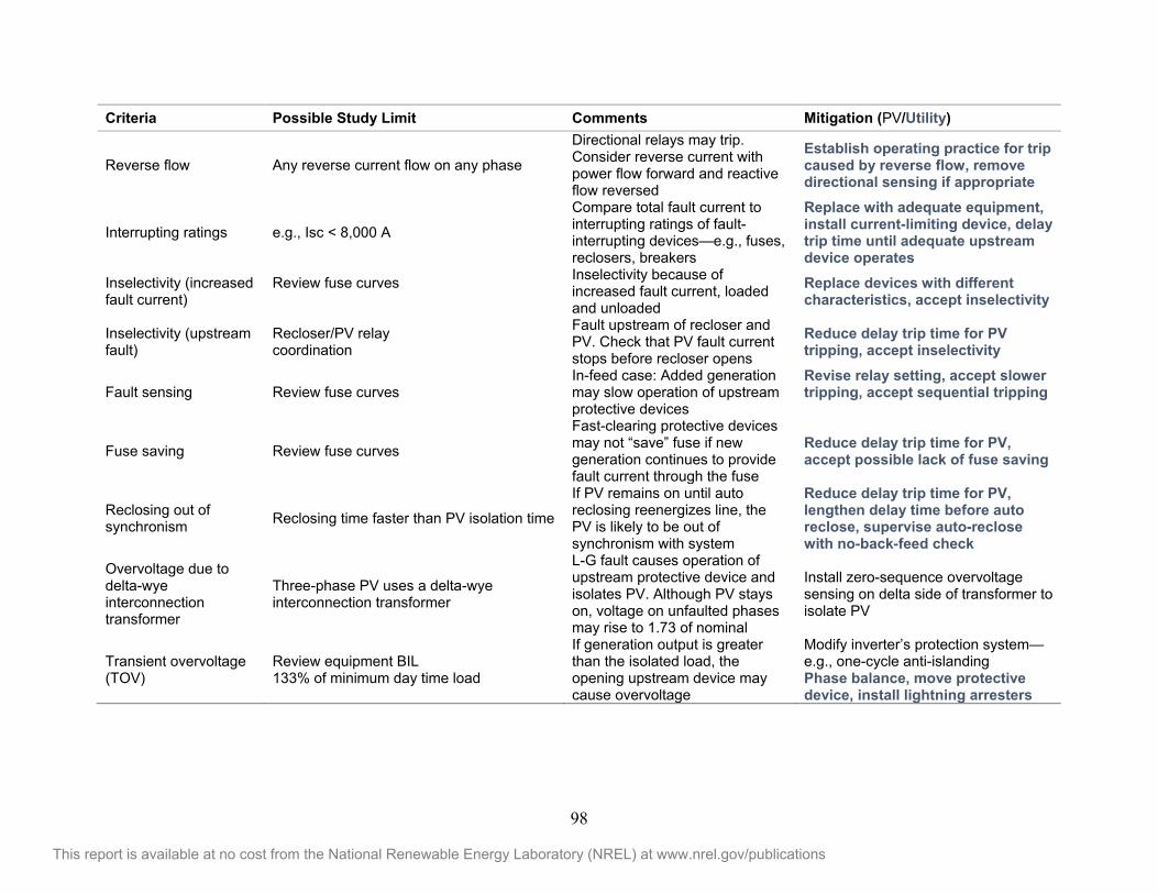
98
This report is available at no cost from the National Renewable Energy Laboratory (NREL) at www.nrel.gov/publications
Criteria Possible Study Limit Comments Mitigation (PV/Utility)
Reverse flow Any reverse current flow on any phase
Directional relays may trip. Consider reverse current with power flow forward and reactive flow reversed
Establish operating practice for trip caused by reverse flow, remove directional sensing if appropriate
Interrupting ratings e.g., Isc < 8,000 A
Compare total fault current to interrupting ratings of fault-interrupting devices—e.g., fuses, reclosers, breakers
Replace with adequate equipment, install current-limiting device, delay trip time until adequate upstream device operates
Inselectivity (increased fault current)
Review fuse curves
Inselectivity because of increased fault current, loaded and unloaded
Replace devices with different characteristics, accept inselectivity
Inselectivity (upstream fault)
Recloser/PV relay coordination
Fault upstream of recloser and PV. Check that PV fault current stops before recloser opens
Reduce delay trip time for PV tripping, accept inselectivity
Fault sensing Review fuse curves In-feed case: Added generation may slow operation of upstream protective devices
Revise relay setting, accept slower tripping, accept sequential tripping
Fuse saving Review fuse curves
Fast-clearing protective devices may not “save” fuse if new generation continues to provide fault current through the fuse
Reduce delay trip time for PV, accept possible lack of fuse saving
Reclosing out of synchronism Reclosing time faster than PV isolation time
If PV remains on until auto reclosing reenergizes line, the PV is likely to be out of synchronism with system
Reduce delay trip time for PV, lengthen delay time before auto reclose, supervise auto-reclose with no-back-feed check
Overvoltage due to delta-wye interconnection transformer
Three-phase PV uses a delta-wye interconnection transformer
L-G fault causes operation of upstream protective device and isolates PV. Although PV stays on, voltage on unfaulted phases may rise to 1.73 of nominal
Install zero-sequence overvoltage sensing on delta side of transformer to isolate PV
Transient overvoltage (TOV)
Review equipment BIL 133% of minimum day time load
If generation output is greater than the isolated load, the opening upstream device may cause overvoltage
Modify inverter’s protection system—e.g., one-cycle anti-islanding Phase balance, move protective device, install lightning arresters
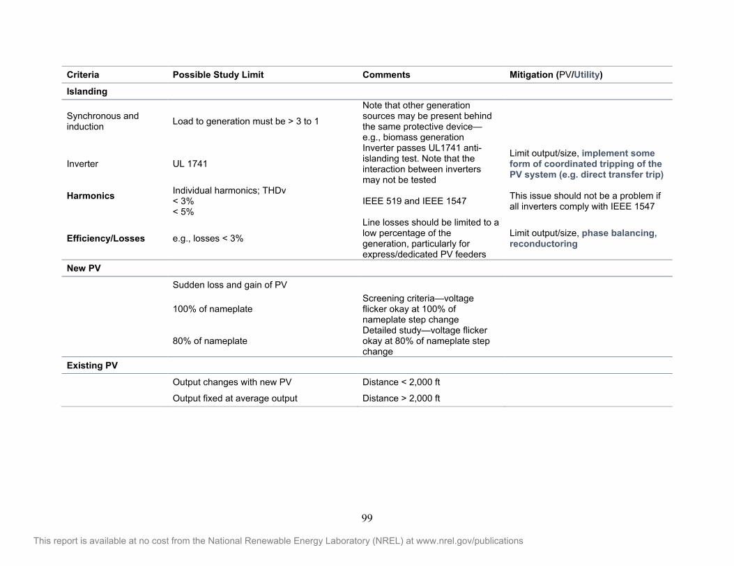
99
This report is available at no cost from the National Renewable Energy Laboratory (NREL) at www.nrel.gov/publications
Criteria Possible Study Limit Comments Mitigation (PV/Utility)
Islanding
Synchronous and induction Load to generation must be > 3 to 1
Note that other generation sources may be present behind the same protective device—e.g., biomass generation
Inverter UL 1741
Inverter passes UL1741 anti-islanding test. Note that the interaction between inverters may not be tested
Limit output/size, implement some form of coordinated tripping of the PV system (e.g. direct transfer trip)
Harmonics
Individual harmonics; THDv < 3% < 5%
IEEE 519 and IEEE 1547 This issue should not be a problem if all inverters comply with IEEE 1547
Efficiency/Losses e.g., losses < 3%
Line losses should be limited to a low percentage of the generation, particularly for express/dedicated PV feeders
Limit output/size, phase balancing, reconductoring
New PV
Sudden loss and gain of PV
100% of nameplate Screening criteria—voltage flicker okay at 100% of nameplate step change
80% of nameplate Detailed study—voltage flicker okay at 80% of nameplate step change
Existing PV
Output changes with new PV Distance < 2,000 ft
Output fixed at average output Distance > 2,000 ft