Embed Size (px)
Citation preview
www.CalSolarResearch.ca.gov
Final Project Report:
Tools Development for Grid Integration of High PV
Penetration
Grantee: DNV ● GL
March 2016
California Solar Initiative
Research, Development, Demonstration and Deployment Program RD&D:
PREPARED BY
DNV GL - Energy Power System Planning 2420 Camino Ramon, Suite 300 San Ramon, CA 94583
Principal Investigator: Ronald Davis [email protected] 925-327-3015
Project Partners: Sacramento Municipal Utility District Hawaii Electric Company Pacific Gas & Electric City of Roseville, California
PREPARED FOR
California Public Utilities Commission California Solar Initiative: Research, Development, Demonstration, and Deployment Program
CSI RD&D PROGRAM MANAGER
Program Manager: Smita Gupta Smita.Gupta @ itron.com
Project Manager: William Marin William.Marin @ itron.com
Additional information and links to project related documents can be found at http://www.calsolarresearch.ca.gov/Funded-Projects/
DISCLAIMER “Any opinions, findings, and conclusions or recommendations expressed in this material are those of the author(s) and do not necessarily reflect the views of the CPUC, Itron, Inc. or the CSI RD&D Program.”

Preface The goal of the California Solar Initiative (CSI) Research, Development, Demonstration, and Deployment (RD&D) Program is to foster a sustainable and self-supporting customer-sited solar market. To achieve this, the California Legislature authorized the California Public Utilities Commission (CPUC) to allocate $50 million of the CSI budget to an RD&D program. Strategically, the RD&D program seeks to leverage cost-sharing funds from other state, federal and private research entities, and targets activities across these four stages:
• Grid integration, storage, and metering: 50-65% • Production technologies: 10-25% • Business development and deployment: 10-20% • Integration of energy efficiency, demand response, and storage with photovoltaics (PV)
There are seven key principles that guide the CSI RD&D Program:
1. Improve the economics of solar technologies by reducing technology costs and increasing system performance;
2. Focus on issues that directly benefit California, and that may not be funded by others; 3. Fill knowledge gaps to enable successful, wide-scale deployment of solar distributed
generation technologies; 4. Overcome significant barriers to technology adoption; 5. Take advantage of California’s wealth of data from past, current, and future installations to
fulfill the above; 6. Provide bridge funding to help promising solar technologies transition from a pre-commercial
state to full commercial viability; and 7. Support efforts to address the integration of distributed solar power into the grid in order to
maximize its value to California ratepayers.
For more information about the CSI RD&D Program, please visit the program web site at www.calsolarresearch.ca.gov.
KEMA Inc. Page v
Table of contents
EXECUTIVE SUMMARY .......................................................................................................... 1
1 INTRODUCTION ...................................................................................................... 4
2 PROJECT GOALS AND METHODOLOGY ....................................................................... 6
2.1 Organization of Project ............................................................................................ 6
2.2 Goals and Objectives ............................................................................................... 6
2.3 Tools ..................................................................................................................... 8
2.4 Modeling and Study Approach .................................................................................. 9
2.5 Evaluation Criteria ................................................................................................ 15
3 RESULTS AND OUTCOMES ..................................................................................... 18
3.1 Hawaiian Electric Grid Company Grid Distribution Studies .......................................... 18
3.2 MECO transmission grid study ................................................................................ 29
3.3 Molokai transmission grid study .............................................................................. 31
3.4 Hawaii Electric Light Company Transmission Study ................................................... 34
3.5 Sacramento Municipal Utility District (SMUD) cases ................................................... 38
3.6 City of Roseville .................................................................................................... 50
3.7 PG&E Cases ......................................................................................................... 55
4 OVERALL CONCLUSIONS AND RECOMMENDATIONS .................................................. 71
5 WHAT IS THE VALUE TO CALIFORNIA UTILITIES ...................................................... 72
6 WHAT IS THE VALUE TO RESIDENTIAL, COMMERCIAL AND INDUSTRIAL RATEPAYERS .. 73
7 OUTREACH .......................................................................................................... 74
KEMA Inc. Page vi
List of tables
Table 1. Technical Criteria for Steady-State Analysis .......................................................................... 16 Table 2. Technical Criteria for Dynamic Analysis ................................................................................ 17 Table 3. Excerpt of Electrical Clusters List organized by data priority .................................................... 22 Table 4. HELCO Generating Mix ....................................................................................................... 34 Table 5. Case description for daytime minimum and maximum peak load conditions .............................. 35 Table 6. Case description for future PV scenarios during minimum daytime peak load conditions ............. 36 Table 7. Result summary for thermal and voltage violations under normal operating conditions during
minimum daytime peak load ............................................................................................................ 36 Table 8. Number of buses facing over voltage during minimum daytime peak load for existing PV and future PV scenarios under normal operating conditions ................................................................................. 37 Table 9. Impacts of Central Solar Plants ........................................................................................... 42 Table 10. Impacts of Central Solar Plants on LTC Operations ............................................................... 43 Table 11. Impacts of High Distributed Solar Penetrations on Feeder Voltage and Backfeed ...................... 43 Table 12 Marginal Houses PV Impact Case Description ......................................................................... 46 Table 13. Annual Curtailment Hours Estimation ................................................................................. 46 Table 14. Annual Curtailed Energy kWh ............................................................................................ 47 Table 15. Solar Panel Estimated Benefit ............................................................................................ 49 Table 16. Estimated Costs of Mitigation Measures for 8kW Solar Panel .................................................. 49 Table 17. Feeder peak load ............................................................................................................. 55 Table 18. Feeder 4 Characteristics ................................................................................................... 57 Table 19. Feeder 4 voltage results ................................................................................................... 70 Table 20: Outreach activities ............................................................................................................ 74
List of figures
Figure 1. Graphical Representation of the Proactive Modeling Approach .................................................. 2 Figure 2. Graphical Representation of the Proactive Modeling Approach ................................................ 10 Figure 3. Modeling representation of equivalent load and aggregated distributed generation for transmission level analysis.................................................................................................................................. 12 Figure 4. Typical single-line view compared to b) geographical view of distribution circuits ...................... 13 Figure 5. Detailed Feeder Model representation of a single distribution circuit and associated distributed roof-top PV systems shown in green.................................................................................................. 14 Figure 6. Geographical representation of distribution feeders, b) comparison of the distribution feeder (electrical lines circled in red) and electrical cluster (all lines circled in black) ......................................... 14 Figure 7. Map of the Hawaiian Islands .............................................................................................. 18 Figure 8. Three Electrical Clusters identified for evaluation studies ....................................................... 19 Figure 9. Detailed Feeder Model representation of a single distribution circuit and associated distributed
roof-top PV systems shown in green.................................................................................................. 20 Figure 10. Graphical representation of the complete utility-owned distribution system and an extract of a cluster study area in callout box ....................................................................................................... 20 Figure 11. Cluster B Feeder Map ...................................................................................................... 21 Figure 12. Cluster B PV Locations ..................................................................................................... 21 Figure 13. Electrical Cluster B Distribution Circuit Results .................................................................... 24 Figure 14. Electrical Cluster B Transformer Results ............................................................................. 25 Figure 15. Dynamic Model Architecture includes Distribution Level representation in the Transmission Model .................................................................................................................................................... 26 Figure 16. Frequency Results from Dynamic Analyses ......................................................................... 27 Figure 17. Molokai Aerial Map .......................................................................................................... 32 Figure 18. 69kV and 12kV Model in Synergi Electric ........................................................................... 39 Figure 19. Reconstructed One-Line Diagram based on Synergi Model ................................................... 40 Figure 20. Example CYMDIST Electrically coupled generator model ...................................................... 55 Figure 21. Feeder 4 Base case load flow CYMDIST results ................................................................... 58 Figure 22. Feeder 4 Base case load flow CYMDIST results: Voltage Profile from substation to Point .......... 59
KEMA Inc. Page vii
Figure 23. Feeder 4 Base case load flow CYMDIST results: Voltage Profile from substation to Point 2 ....... 60 Figure 24. Feeder 4 Base case load flow CYMDIST results: Voltage Profile from substation to Point 3 ....... 61 Figure 25. Feeder 4 100% Penetration case load flow CYMDIST results ................................................. 62 Figure 26. Feeder 4 100% Penetration case load flow CYMDIST results: Voltage Profile from substation to Point 1 .......................................................................................................................................... 63 Figure 27. Feeder 4 100% Penetration case load flow CYMDIST results: Voltage Profile from substation to Point 2 .......................................................................................................................................... 64 Figure 28. Feeder 4 100% Penetration case load flow CYMDIST results: Voltage Profile from substation to Point 3 .......................................................................................................................................... 65 Figure 29. Feeder 4 Voltage recovery feeder voltage at 100% PV penetration ........................................ 66 Figure 30. Feeder 4 Voltage recovery feeder voltage at 100% PV penetration: Voltage Profile from
substation to Point 1 ....................................................................................................................... 67 Figure 31. Feeder 4 Voltage recovery feeder voltage at 100% PV penetration: Voltage Profile from substation to Point 2 ....................................................................................................................... 68 Figure 32. Feeder 4 Voltage recovery feeder voltage at 100% PV penetration: Voltage Profile from substation to Point 3 ....................................................................................................................... 69
KEMA Inc. Page viii
List of abbreviations
Abbreviation Meaning
BEW Behnke, Erdman and Whitaker
c.kVA Connected kVA
CEC California Energy Commission
CPUC California Public Utilities Commission
CSI California Solar Initiative
CT Current Transformer
DG Distributed Generation
DNV GL Det Norske Veritas Germanischer Lloyd
EPRI Electric Power Research Institute
GIS Geographical Information System
HECO Hawaiian Electric Company
HELCO Hawaiian Electric Light Company
Hi-PV High Penetration Photovoltaic
IEEE Institute of Electrical and Electronics Engineers
IRS Interconnection Requirements Study
LDC Line Drop Compensation
LLNL Lawrence Livermore National Laboratory
LTC Load Tap Changer
LVA Locational Value Analysis
LVM Locational Value Mapping
MECO Maui Electric Company
NERC North American Reliability Corporation
PG&E Pacific Gas & Electric
PSLF Positive Sequence Load Flow
PSS/E Power System Simulation for Engineers
PT Potential Transformer
PV Photovoltaic
RD&D Research, Development & Deployment
SLACA Substation Load and Capacity Analysis
SMUD Sacramento Municipal Utility District
T&D Transmission & Distribution
UL Underwriters Laboratories
VR Voltage Regulator
WECC Western Electricity Coordinating Council
DNV GL – Document No.:84340790-FSE-R-01-A - www.dnvgl.com Page -1
EXECUTIVE SUMMARY
In 2012, DNV GL was awarded a two year grant from the California Public Utility Commission (CPUC) under
the California Solar Initiative (CSI) Research, Development and Deployment (RD&D) Solicitation 3. The title
of the project was “Tools Development for Grid Integration of High PV Penetration”. Itron was the CPUC
RD&D Program Administrator. This project builds on the Sacramento Municipal Utility District (SMUD)
Solicitation 1 titled “High Penetration PV Project (Hi-PV) Impacts to Transmission and Distribution Grids” to
develop tools and methodologies to study distributed PV and central solar plants impacts on the utility grids.
The team members were Hawaii Electric Company (HECO), SMUD, Pacific Gas & Electric (PG&E), and City of
Roseville, California. The objectives of Solicitation 3 were to continue the studies on the potential impacts of
distributed solar on the distribution grids and the development of a study methodology that any electric
utility can incorporate into the planning process.
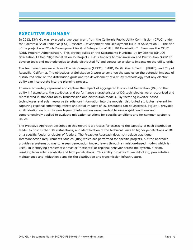
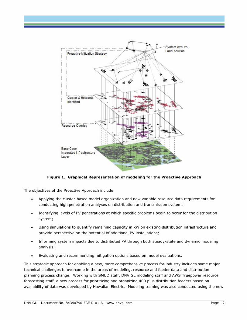
To more accurately represent and capture the impact of aggregated Distributed Generation (DG) on the
utility infrastructure, the attributes and performance characteristics of DG technologies were recognized and
represented in standard utility transmission and distribution models. By factoring inverter-based
technologies and solar resource (irradiance) information into the models, distributed attributes relevant for
capturing regional smoothing effects and cloud impacts of DG resources can be assessed. Figure 1 provides
an illustration on how the new layers of information were overlaid to assess grid conditions and
comprehensively applied to evaluate mitigation solutions for specific conditions and for common systemic
issues.
The Proactive Approach described in this report is a process for assessing the capacity of each distribution
feeder to host further DG installations, and identification of the technical limits to higher penetrations of DG
on a specific feeder or cluster of feeders. The Proactive Approach does not replace traditional
Interconnection Requirements Studies (IRS) which are performed for specific projects, but the approach
provides a systematic way to assess penetration impact levels through simulation-based models which is
useful in identifying problematic areas or “hotspots” or regional behavior across the system, a priori,
resulting from solar variability and high penetrations. This ability provides forward-looking, preventative
maintenance and mitigation plans for the distribution and transmission infrastructure.
DNV GL – Document No.:84340790-FSE-R-01-A - www.dnvgl.com Page -2
Figure 1. Graphical Representation of modeling for the Proactive Approach
The objectives of the Proactive Approach include:
Applying the cluster-based model organization and new variable resource data requirements for
conducting high penetration analyses on distribution and transmission systems
Identifying levels of PV penetrations at which specific problems begin to occur for the distribution
system;
Using simulations to quantify remaining capacity in kW on existing distribution infrastructure and
provide perspective on the potential of additional PV installations;
Informing system impacts due to distributed PV through both steady-state and dynamic modeling
analysis;
Evaluating and recommending mitigation options based on model evaluations.
This strategic approach for enabling a new, more comprehensive process for industry includes some major
technical challenges to overcome in the areas of modeling, resource and feeder data and distribution
planning process change. Working with SMUD staff, DNV GL modeling staff and AWS Truepower resource
forecasting staff, a new process for prioritizing and organizing 400 plus distribution feeders based on
availability of data was developed by Hawaiian Electric. Modeling training was also conducted using the new

DNV GL – Document No.:84340790-FSE-R-01-A - www.dnvgl.com Page -3
tools to support adoption of new capabilities and confidence building to gain traction. While the change
process was still in progress, the Proactive Approach as documented in this report demonstrates a viable
and consistent pathway for renewable integration and grid modernization needs.
Supporting the level of change resulting from high penetrations of distributed resources on the grid requires
development of the following capabilities:
Enhanced modeling tools,
Consistent screening and evaluation procedures,
Common queue to prioritize studies, and
Analysis capability to factor in new resource information and handle the increased volume of
customer demand on a timely basis.
This report describes the studies conducted by each of the four electric utilities who selected feeders of
different line lengths, line characteristics, and customer mix and customer load/PV locations that could
potentially limit the amount of solar that could be installed on the feeders. Each utility developed specific
study objectives such as determining individual solar limits per feeder; solar limits on a large substation with
more than 69 feeders, mitigation measures, voltage impacts under solar shut down and start up; and impact
on line regulators and capacitor banks on long distribution feeders.
Before undertaking this study, it was believed that feeders could be grouped into similar profiles to reduce
the need to conduct studies on every distribution feeder. However, every feeder has unique and different
line characteristics and load distributions that make it difficult to group feeders in classifications.
For each utility, this report will have one or two examples of the feeder analyses undertaken. The full utility
reports can be found on the CPUC CSI RD&D website at http://www.casloarresearch.ca.gov

DNV GL – Document No.:84340790-FSE-R-01-A - www.dnvgl.com Page -4
1 INTRODUCTION
In 2012, DNVGL was awarded a two year contract from the California Public Utility Commission (CPUC)
under the California Solar Initiative (CSI) Research, Development and Deployment (RD&D) Solicitation 3.
The title of the project was “Tools Development for Grid Integration of High PV Penetration”. Itron was the
CPUC RD&D Program Administrator. This project builds on the Sacramento Municipal Utility District (SMUD)
Solicitation 1 project titled “High Penetration PV Project (Hi-PV) Impacts to Transmission and Distribution
Grids” to develop tools and methodologies to study distributed PV and central solar plants impacts on the
utility grids.
The team members were Hawaii Electric Company (HECO), SMUD, Pacific Gas & Electric (PG&E), and City of
Roseville, California. The objectives of Solicitation 3 were to continue the studies on the potential impacts of
distributed solar on the distribution grids and the development of a study methodology that any electric
utility can incorporate into the planning process.
This report is a summary of the work conducted on the utilities’ distribution grids. On the CPUC CSI RD&D
website, there are additional reports on the specific tasks completed for each utility.
http://www.calsolarresearch.ca.gov/funded-projects/85-tools-development-for-grid-integration-of-high-pv-penetration
The reports are listed below:
City of Roseville: Westplan Solar Penetration Final Report SMUD: Substation EG High PV Penetration Study, Transmission, Substation, and Feeder Study SMUD: PV High Penetration Mitigation Study HECO: CSI3 Proactive Approach Cluster Circuit Analysis HECO: CSI3 Circuit Evaluation and Selection
HECO: CSI3 Cluster Evaluation Methodology
PG&E: Report on Solar Grid Integration Final Report
The research and demonstration on the impacts of high penetrations of renewable resources began in 2003
with the California Energy Commission (CEC) sponsored Locational Value Analysis (LVA) of renewable
resources on the transmission grid. BEW Engineering (BEW) developed the methodology and software tools
under a CEC contract (CEC-2005-500-106) to integrate a transmission power flow model with a
Geographical Information Systems (GIS) mapping tool to find optimal locations for renewable resources to
reduce or eliminate transmission congestion. The project was expanded under another CEC project (CEC-
500-2007) to study the impacts of high penetrations of California installed wind and solar projects.
In 2008 through 2010, BEW worked with Itron and Lawrence Livermore National Laboratory (LLNL) to
expand the LVA to investigate the economic and operational value of high penetrations of distributed
generation on the distribution grid. The Itron projects with BEW as a subcontractor (CPUC Self Generation
Incentive Program-Sixth Year Impact Evaluation, August 2007 and CPUC Self Generation Incentive Program
– Optimizing Dispatch and Location of Distributed Generation, July 2010) evaluated the benefits of existing
distributed generation installed under the California Self Generation Incentive Program. The LLNL Project
(CEC-500-2011-026) expanded the results of these two projects to study the economic and operational
value of installing high penetrations of various types of distributed generation on the distribution grid such
as cogeneration, solar, small wind, biomass, fuel cells, etc. All of these studies analyzed the major
California electric utility systems.
Under the SMUD CPUC CSI RDD#1 contract and separate BEW contracts with HECO, BEW began developing
detailed distribution feeder power flow simulation data sets for Synergi Electric, Power World Simulator,
DNV GL – Document No.:84340790-FSE-R-01-A - www.dnvgl.com Page -5
PSLF, PSS/E and PSS/Sincal. The data sets were prepared for both unbalanced and balanced feeder
representations. For each utility system, individual single-phase and three-phase PV inverters were modeled
in the data sets. For HECO, the number of distributed PV inverters was over 4,000. There were 19
distribution feeders developed for Oahu, Maui and Big Island and 11 distribution feeders for SMUD that
include a solar community, rural area with a long feeder and a digester, part of a large residential area and
several other feeders. HECO has existing feeders with PV penetrations over 50%. BEW studied these
feeders to determine the potential impacts from such high penetrations.
HECO has a mandate of 40% renewable penetration by 2025. SMUD and the other California electric
utilities have mandates of 33% penetration of renewables by 2020. These renewable resources can be any
combination of hydroelectric (under 30 MW generating capacity or smaller), biomass, wind, solar and
geothermal. Initially, renewable resources could be located in-state and out-of-state. A revised state
mandate sets a percentage limit for in-state renewables. The construction of long high-voltage transmission
lines to move power from remote areas to load centers was costly with long construction and permitting lead
times. To counter this cost, the utilities began to facilitate the installation of distributed PV on the
distribution feeders and behind the customer meters. While this reduces the need for costly transmission
lines, it does create new problems for old distribution grids that were designed to move power from the
substation to the customer load. The distribution system was never designed to move power from the
customer to the transmission grid (reverse power flows) over the distribution feeder.
DNV GL – Document No.:84340790-FSE-R-01-A - www.dnvgl.com Page -6
2 PROJECT GOALS AND METHODOLOGY
2.1 Organization of Project
The CPUC CSI RDD CSI Solicitation #3 was divided into distinct objectives: (1) Project Management; (2)
Utility Interconnection: Nodal Approach for Strategically Locating PV; (3) Grid Operations: Case Studies of
Evaluating Distributed PV on Distribution Grids.
BEW Engineering was the original leader of the project until the company was acquired by DNV GL. DNV GL
was the new leader of the team comprised of western utilities in developing, validating and demonstrating
the methodologies and software tools to enable reliable integration of increasing levels of “as-available”
distributed PV. The team includes SMUD, the Hawaii Electric Companies, PG&E, City of Roseville and DNV
GL. The Hawaii Electric Company is comprised of Hawaii Electric Company (HECO), Maui Electric Company
(MECO), and Hawaii Electric Light Company (HELCO).
The first objective was to expand upon previous California Energy Commission and California Public Utility
Commission Projects. Transmission simulation tools define both congestion zones and optimal locations for
new generation through map overlays of renewable resource potentials across the transmission grid. This
objective integrates the distribution grid with a visual mapping tool (i.e. GIS compatible platform specified
by the utility) into an expanded locational value methodology. The approach assesses impacts across the
system from a strategic development and grid enhancement perspective. California Rule 21 and Hawaii Rule
14H sets guidelines and “triggers” in analyzing PV installations but not implementation. The methodology
and process was used by utilities to facilitate distributed renewable resource expansion without negatively
impacting system performance.
The second objective was to develop a validation approach to evaluate PV integration. Studies were carried
out on potential impacts to individual feeders, substations, utility regions and utility grids from high
Distributed Generation (DG) PV penetrations. The participating utilities select different feeder
configurations to demonstrate, evaluate and validate high PV penetrations under steady-state, contingency
and dynamic scenarios. This objective was to document the ability of the software tools to study PV
integration.
2.2 Goals and Objectives
Task 1: Project Management
Schedule and coordinate the principal participants and subcontractors
Prepare monthly reports and issue draft and final reports
Schedule workshops, outreach programs, and technology transfers
DNV GL – Document No.:84340790-FSE-R-01-A - www.dnvgl.com Page -7
Task 2: Nodal Approach for Strategically Locating PV
Expand the CEC Locational Value Mapping to include utility distribution feeders to find potential
areas on the distribution feeders for distributed PV injection based on a transmission nodal
approach. Develop detailed input into distribution and transmission power flow models with the
capability of simulating the system and generating maps of congestion or problem areas.
Integrate a global, GIS-based mapping tool to overlay strategic nodes (distribution feeder cluster)
locations onto a geographic representation of the system to analyze potential impacts of PV
locations.
Develop an interface tool to transfer data between distribution modeling tools (single phase,
unbalanced) and transmission system level balanced power simulation tools to enable utility
planners to use their own respective models for studies.
Develop the methodology for the utility to use to evaluate the potential impacts and contributions of
DG PV to fault current, frequency, voltage, protection coordination, contingency outages, harmonics,
flicker, etc.
Task 3: Grid Operations: Evaluating Distributed PV on Distribution Grids
Select utility feeder configurations comprised of various customer mixes, feeder lengths, feeder
elements (capacitor banks, regulators, cogeneration, other DG units,), etc. to evaluate the potential
impacts of high penetration of inverters on distribution system performance. System studies include
voltage, frequency, ramping, harmonics, fault current, reverse power flow, protection, and other
parameters. The objective was to evaluate the different potential limitations to PV development and
determine which elements were the most important by analyzing a wide variety of feeder
configurations.
Evaluate the criteria in California Rule 21 and subsequent upcoming changes, Hawaii Rule 14H and
other industry standards/regulations (IEEE 1547, UL, NERC IVGTF, WECC) to determine how these
regulations impact PV expansion and distribution system performance. For example, Rule 21 and
Rule 14H set a PV penetration of 15% on a feeder to trigger a detailed study. Another example is
the percent change in fault current with PV installations. The goal was the study of various feeder
types to help in forming guideline development for utilities to assess high penetration PV issues that
require consideration of new target levels and design rules. It was advantageous for the western
utilities to have agreement and recommendations on guidelines for developers and agencies to guide
new processes and inform development of more appropriate criteria and study parameters.
With Hawaii utilities having feeders with over 50% PV penetration at the start of this study, the
lessons learned about ramping, reliability and operations and distribution planning can be applied to
California to plan ahead of potential problems and develop viable solutions.
Determine the next PV inverter operating requirements such as voltage support, VAR generation,
frequency changes, reserve contribution, ramping, etc. for single-phase and three-phase inverters.
For example, Hawaii was investigating an under frequency trip of 57 Hz for ride through capability
for three-phase PV installations only.
DNV GL – Document No.:84340790-FSE-R-01-A - www.dnvgl.com Page -8
Integration of different distribution system analysis tools which demonstrates the methodology can
be applied to different software. Examples of software include: Synergi Electric, Cooper Power
Systems CYME and Siemens PSS/Sincal.
2.3 Tools
Various tools were used in this report, demonstrating that the methodology is not software-specific. Synergi
Electric and CYME were used for steady-state or quasi-static distribution system analysis. PowerWorld
Simulator was used in this case for steady-state transmission system analysis, and PSS/E and PSLF were
used for both steady-state and dynamic analysis of the transmission system.
Simulation-based models were used to design and assess the system or any part of the network under
different steady-state and time variant conditions, as introduced by those running the model(s). System
network stability was one of the most important criteria for maintaining reliability and represents how stable
the system remains due to sudden changes or disturbances. Models were used to represent the system
response under steady-state and dynamic (time transient) conditions. The following were two types of
simulations used in this analysis:
1. Steady state simulations capture the system equilibrium conditions, or how stable the system is
in response to small and slow changes. Most component design specifications are listed for steady-
state operations. Steady state simulations can thus look to model the output of PV systems on 1) a
clear sunny day compared to 2) a cloudy day condition. Quasi-static simulations can also be run
using the same software to simulate transient events such as clouds passing over the area, which
results in a rapid decrease or increase in PV output.
2. Dynamic analysis looks at time-variant and continuous change due to load or generation in normal
and non-normal (contingency) conditions. Dynamic studies capture detailed change response over a
period of time for the system ranging from faults and recovery to normal conditions. For high
penetration PV systems, dynamic simulations are useful to assess system response due to voltage,
current and frequency change in transient conditions (sub-seconds to seconds) or to ramp conditions
lasting minutes to hours. Thus dynamic analysis is often the most data and model intensive. As
such dynamic modeling requires very accurate model representations and validation data from the
actual infrastructure including details such as relays, inverters, line impedances, switching,
measured solar conditions and geographic locations.
o Transient simulations are a subset of dynamic analysis that looks at transitory or very short,
time-variant change events such as a fault (i.e. line or generator). Transient stability studies for
example, assess how quickly the system returns to stable conditions after a sudden fault or
change over a prescribed time interval (ranging from sub-seconds to tens of seconds).
DNV GL – Document No.:84340790-FSE-R-01-A - www.dnvgl.com Page -9
2.4 Modeling and Study Approach
To more accurately represent and capture the impact of aggregated DG on the utility infrastructure, the
attributes and performance characteristics of DG technologies were recognized and represented in standard
utility transmission and distribution models. By factoring inverter-based technologies and solar resource
(irradiance) information into the models, distributed attributes relevant for capturing regional smoothing
effects and cloud impacts of DG resources can be assessed. Figure 2 provides an illustration on how the new
layers of information were overlaid to assess grid conditions and comprehensively applied to evaluate
mitigation solutions for specific conditions and for common systemic issues.
The Proactive Approach provides a systematic way to assess penetration impact levels through simulation-
based models which is useful in identifying problematic areas or “hotspots” or regional behavior across the
system, a priori, resulting from solar variability and high penetrations. This ability provides forward-looking,
preventative maintenance and mitigation plans for the distribution and transmission infrastructure. The
Proactive Approach does not replace traditional Interconnection Requirements Studies (IRS) which are used
for specific projects and tasks.

DNV GL – Document No.:84340790-FSE-R-01-A - www.dnvgl.com Page -10
Figure 2. Graphical Representation of modeling for the Proactive Approach
The objectives of the Proactive Approach include:
Applying the cluster-based model organization and new variable resource data requirements for
conducting high penetration analysis on distribution and transmission systems
Identifying levels of PV penetration at which specific problems begin to occur for the distribution
system;
Using simulations to quantify remaining capacity in kW on existing distribution infrastructure and
provide perspective on the potential of additional PV installations;
Informing system impacts due to distributed PV through both steady-state and dynamic modeling
analysis;
Evaluating and recommending mitigation options based on model evaluations.
This strategic approach for enabling a new, more comprehensive process for industry includes some major
technical challenges to overcome in the areas of modeling, resource and feeder data and distribution
planning process change. Working with SMUD staff, DNV GL modeling staff and AWS Truepower resource
forecasting staff, a new process for prioritizing and organizing 400 plus distribution feeders based on
DNV GL – Document No.:84340790-FSE-R-01-A - www.dnvgl.com Page -11
availability of data was developed by Hawaiian Electric. Modeling training was also conducted using the new
tools to support adoption of new capabilities and confidence building to gain traction. While the change
process was still in progress, the Proactive Approach as documented in these reports demonstrates a viable
and consistent pathway for renewable integration and grid modernization needs.
Supporting the level of change resulting from high penetrations of distributed resources on the grid requires
development of the following capabilities:
Enhanced modeling tools,
Consistent screening and evaluation procedures,
Common queue to prioritize studies, and
Analysis capability to factor in new resource information and handle the increased volume of
customer demand on a timely basis.
Major enabling milestones leveraged as part of this work include the following enhancements:
Modeling Tools: Enhancing Transmission and Distribution (T&D) Models used by utilities to
consistently account for distributed PV as a generator and not simply negative load. Models now can
directly extract PV systems by location from the GIS and more accurately represent the feeders and
equipment attributes using a consistent Synergi model. Models were also being enhanced to capture
details of new smart inverters as they were made available by the manufacturers.
Monitoring & Analysis Tools: Gain visibility to behind-the-meter PV through monitoring and
resource tracking and to prioritize impacts based on penetration levels. Leveraging grant funding,
HECO has also been developing and sharing information from data tracking and analysis tools such
as the Locational Value Mapping (LVM), REWatch and DGCentral to provide more public
transparency on increasing PV penetrations, change impacts and development queues. Industry and
renewable forecasting data were also helping to better manage changing resource and production
levels in real-time.
Procedures & Techniques: Integrate and implement scenario-based techniques and new tools
into the existing planning and operating practices to confidently and securely accommodate change.
Training was being coordinated and tailored on the new modeling tools, techniques and validation
datasets to support T&D interconnection and operational needs.
DNV GL – Document No.:84340790-FSE-R-01-A - www.dnvgl.com Page -12
2.4.1 Modeling Enhancements
This effort supports application and demonstration of a comprehensive modeling structure for the Proactive
Approach to conduct reliable, cluster-level (regional) and distribution circuit based (local) analysis that can
streamline DG assessment and proactively review high penetration DG impacts on the system. Specifically,
the analysis focuses on customer sited, rooftop PV systems on Oahu and some commercial PV systems
connected to the electrical grid at the 12kV distribution level. Several enhancements were made to support
modeling of high penetration PV.
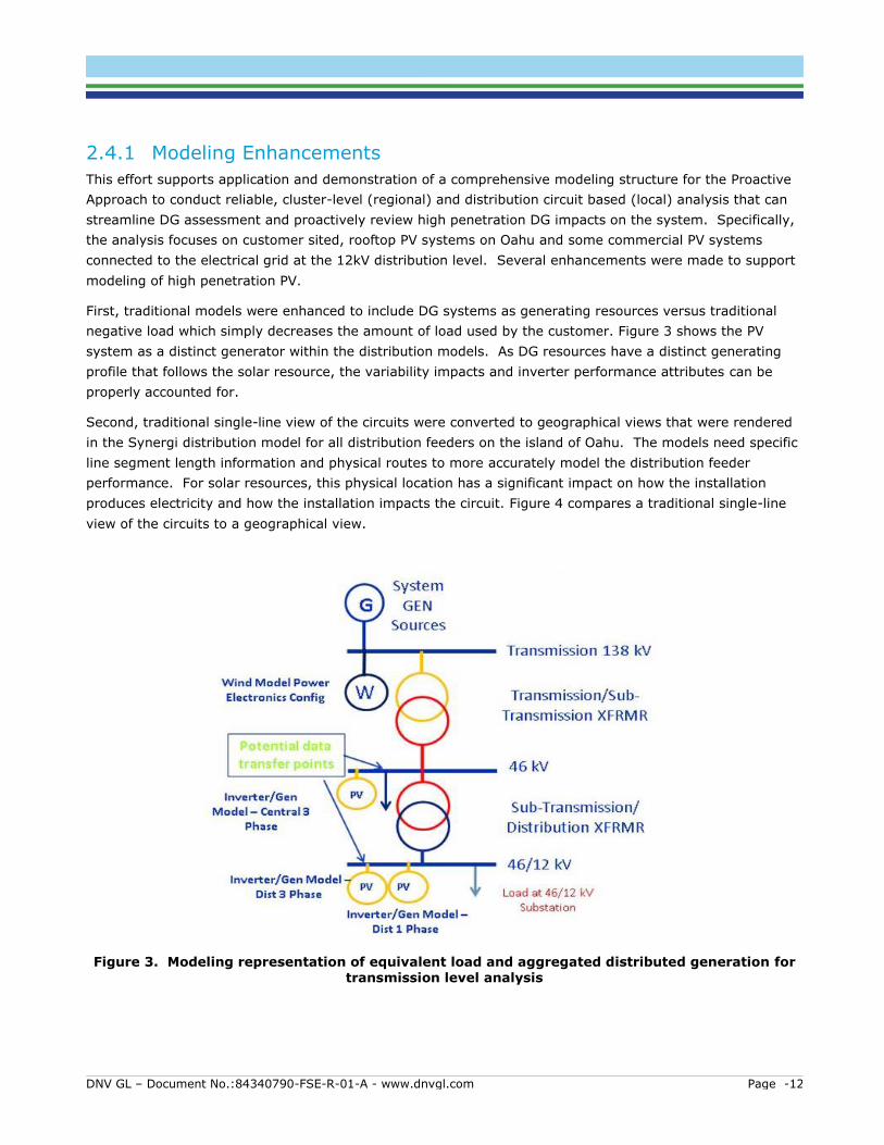
First, traditional models were enhanced to include DG systems as generating resources versus traditional
negative load which simply decreases the amount of load used by the customer. Figure 3 shows the PV
system as a distinct generator within the distribution models. As DG resources have a distinct generating
profile that follows the solar resource, the variability impacts and inverter performance attributes can be
properly accounted for.
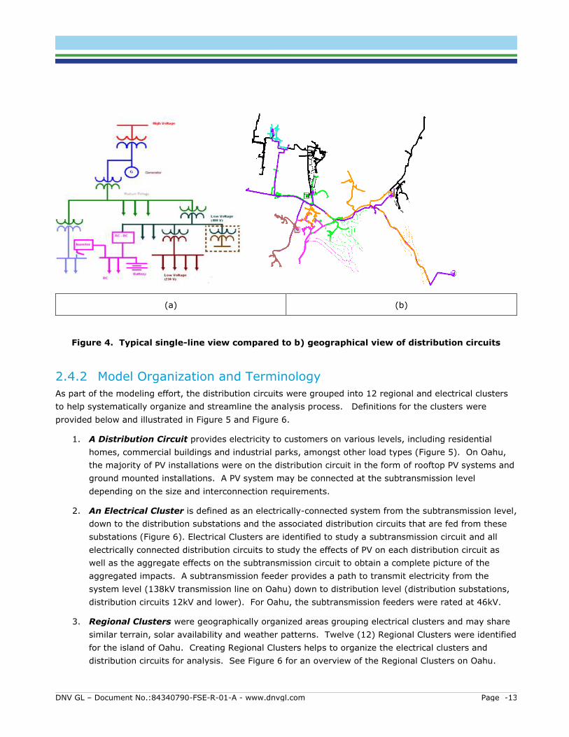
Second, traditional single-line view of the circuits were converted to geographical views that were rendered
in the Synergi distribution model for all distribution feeders on the island of Oahu. The models need specific
line segment length information and physical routes to more accurately model the distribution feeder
performance. For solar resources, this physical location has a significant impact on how the installation
produces electricity and how the installation impacts the circuit. Figure 4 compares a traditional single-line
view of the circuits to a geographical view.
Figure 3. Modeling representation of equivalent load and aggregated distributed generation for transmission level analysis
DNV GL – Document No.:84340790-FSE-R-01-A - www.dnvgl.com Page -13
(a) (b)
Figure 4. Typical single-line view compared to b) geographical view of distribution circuits
2.4.2 Model Organization and Terminology
As part of the modeling effort, the distribution circuits were grouped into 12 regional and electrical clusters
to help systematically organize and streamline the analysis process. Definitions for the clusters were
provided below and illustrated in Figure 5 and Figure 6.
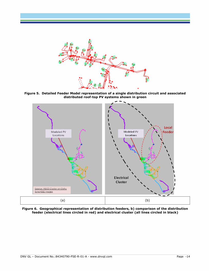
1. A Distribution Circuit provides electricity to customers on various levels, including residential
homes, commercial buildings and industrial parks, amongst other load types (Figure 5). On Oahu,
the majority of PV installations were on the distribution circuit in the form of rooftop PV systems and
ground mounted installations. A PV system may be connected at the subtransmission level
depending on the size and interconnection requirements.
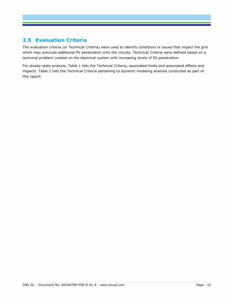
2. An Electrical Cluster is defined as an electrically-connected system from the subtransmission level,
down to the distribution substations and the associated distribution circuits that are fed from these
substations (Figure 6). Electrical Clusters are identified to study a subtransmission circuit and all
electrically connected distribution circuits to study the effects of PV on each distribution circuit as
well as the aggregate effects on the subtransmission circuit to obtain a complete picture of the
aggregated impacts. A subtransmission feeder provides a path to transmit electricity from the
system level (138kV transmission line on Oahu) down to distribution level (distribution substations,
distribution circuits 12kV and lower). For Oahu, the subtransmission feeders were rated at 46kV.
3. Regional Clusters were geographically organized areas grouping electrical clusters and may share
similar terrain, solar availability and weather patterns. Twelve (12) Regional Clusters were identified
for the island of Oahu. Creating Regional Clusters helps to organize the electrical clusters and
distribution circuits for analysis. See Figure 6 for an overview of the Regional Clusters on Oahu.
DNV GL – Document No.:84340790-FSE-R-01-A - www.dnvgl.com Page -14
Figure 5. Detailed Feeder Model representation of a single distribution circuit and associated distributed roof-top PV systems shown in green
(a) (b)
Figure 6. Geographical representation of distribution feeders, b) comparison of the distribution feeder (electrical lines circled in red) and electrical cluster (all lines circled in black)
DNV GL – Document No.:84340790-FSE-R-01-A - www.dnvgl.com Page -15
2.5 Evaluation Criteria
The evaluation criteria (or Technical Criteria) were used to identify conditions or issues that impact the grid
which may preclude additional PV penetration onto the circuits. Technical Criteria were defined based on a
technical problem created on the electrical system with increasing levels of PV penetration.
For steady-state analysis, Table 1 lists the Technical Criteria, associated limits and associated effects and
impacts. Table 2 lists the Technical Criteria pertaining to dynamic modeling analysis conducted as part of
this report.
DNV GL – Document No.:84340790-FSE-R-01-A - www.dnvgl.com Page -16
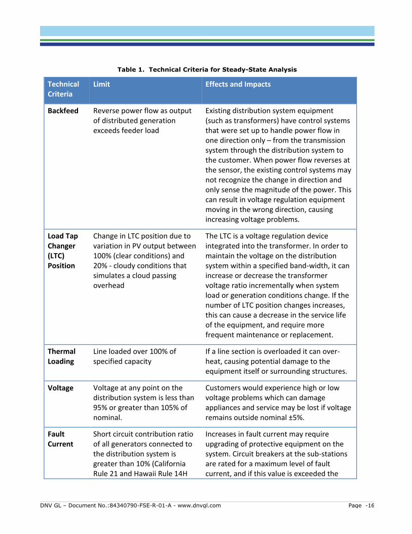
Table 1. Technical Criteria for Steady-State Analysis
Technical Criteria
Limit Effects and Impacts
Backfeed Reverse power flow as output of distributed generation exceeds feeder load
Existing distribution system equipment (such as transformers) have control systems that were set up to handle power flow in one direction only – from the transmission system through the distribution system to the customer. When power flow reverses at the sensor, the existing control systems may not recognize the change in direction and only sense the magnitude of the power. This can result in voltage regulation equipment moving in the wrong direction, causing increasing voltage problems.
Load Tap Changer (LTC) Position
Change in LTC position due to variation in PV output between 100% (clear conditions) and 20% - cloudy conditions that simulates a cloud passing overhead
The LTC is a voltage regulation device integrated into the transformer. In order to maintain the voltage on the distribution system within a specified band-width, it can increase or decrease the transformer voltage ratio incrementally when system load or generation conditions change. If the number of LTC position changes increases, this can cause a decrease in the service life of the equipment, and require more frequent maintenance or replacement.
Thermal Loading
Line loaded over 100% of specified capacity
If a line section is overloaded it can over-heat, causing potential damage to the equipment itself or surrounding structures.
Voltage Voltage at any point on the distribution system is less than 95% or greater than 105% of nominal.
Customers would experience high or low voltage problems which can damage appliances and service may be lost if voltage remains outside nominal ±5%.
Fault Current
Short circuit contribution ratio of all generators connected to the distribution system is greater than 10% (California Rule 21 and Hawaii Rule 14H
Increases in fault current may require upgrading of protective equipment on the system. Circuit breakers at the sub-stations are rated for a maximum level of fault current, and if this value is exceeded the
DNV GL – Document No.:84340790-FSE-R-01-A - www.dnvgl.com Page -17
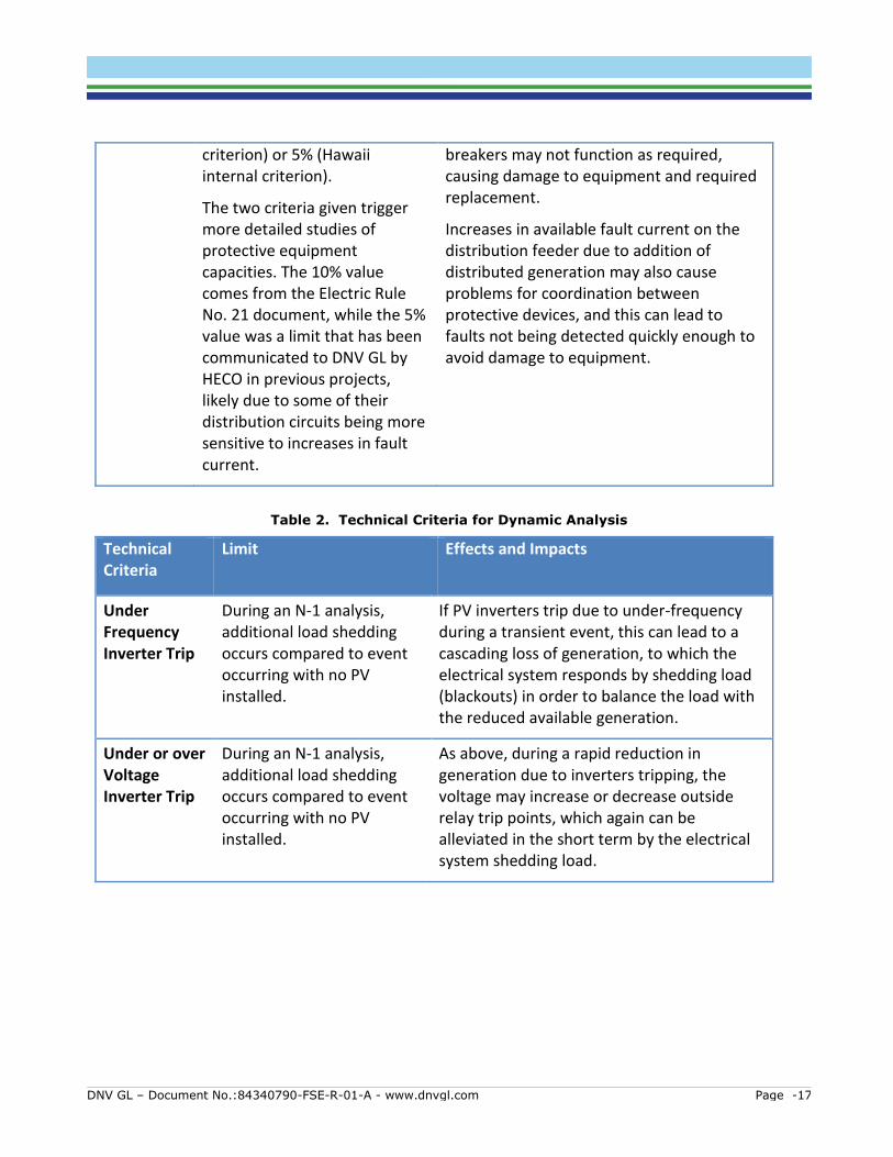
criterion) or 5% (Hawaii internal criterion).
The two criteria given trigger more detailed studies of protective equipment capacities. The 10% value comes from the Electric Rule No. 21 document, while the 5% value was a limit that has been communicated to DNV GL by HECO in previous projects, likely due to some of their distribution circuits being more sensitive to increases in fault current.
breakers may not function as required, causing damage to equipment and required replacement.
Increases in available fault current on the distribution feeder due to addition of distributed generation may also cause problems for coordination between protective devices, and this can lead to faults not being detected quickly enough to avoid damage to equipment.
Table 2. Technical Criteria for Dynamic Analysis
Technical Criteria
Limit Effects and Impacts
Under Frequency Inverter Trip
During an N-1 analysis, additional load shedding occurs compared to event occurring with no PV installed.
If PV inverters trip due to under-frequency during a transient event, this can lead to a cascading loss of generation, to which the electrical system responds by shedding load (blackouts) in order to balance the load with the reduced available generation.
Under or over Voltage Inverter Trip
During an N-1 analysis, additional load shedding occurs compared to event occurring with no PV installed.
As above, during a rapid reduction in generation due to inverters tripping, the voltage may increase or decrease outside relay trip points, which again can be alleviated in the short term by the electrical system shedding load.
DNV GL – Document No.:84340790-FSE-R-01-A - www.dnvgl.com Page -18
3 RESULTS AND OUTCOMES
Section 3 discusses the integration studies conducted for HECO, SMUD, PG&E and City of Roseville.
3.1 Hawaiian Electric Grid Company Grid Distribution Studies
This section contains a description of work carried out to develop and test the Proactive Approach on a
Hawaiian Electric Company electrical cluster on the island of Oahu. This work involved the application of the
methodology to three clusters selected by HECO, and testing and refinement of the processes.
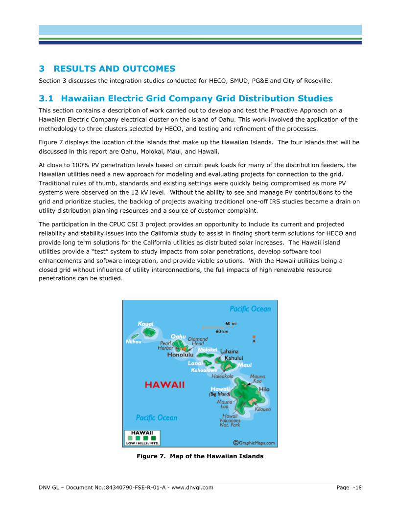
Figure 7 displays the location of the islands that make up the Hawaiian Islands. The four islands that will be
discussed in this report are Oahu, Molokai, Maui, and Hawaii.
At close to 100% PV penetration levels based on circuit peak loads for many of the distribution feeders, the
Hawaiian utilities need a new approach for modeling and evaluating projects for connection to the grid.
Traditional rules of thumb, standards and existing settings were quickly being compromised as more PV
systems were observed on the 12 kV level. Without the ability to see and manage PV contributions to the
grid and prioritize studies, the backlog of projects awaiting traditional one-off IRS studies became a drain on
utility distribution planning resources and a source of customer complaint.
The participation in the CPUC CSI 3 project provides an opportunity to include its current and projected
reliability and stability issues into the California study to assist in finding short term solutions for HECO and
provide long term solutions for the California utilities as distributed solar increases. The Hawaii island
utilities provide a “test” system to study impacts from solar penetrations, develop software tool
enhancements and software integration, and provide viable solutions. With the Hawaii utilities being a
closed grid without influence of utility interconnections, the full impacts of high renewable resource
penetrations can be studied.
Figure 7. Map of the Hawaiian Islands
DNV GL – Document No.:84340790-FSE-R-01-A - www.dnvgl.com Page -19
3.1.1 Description of cases
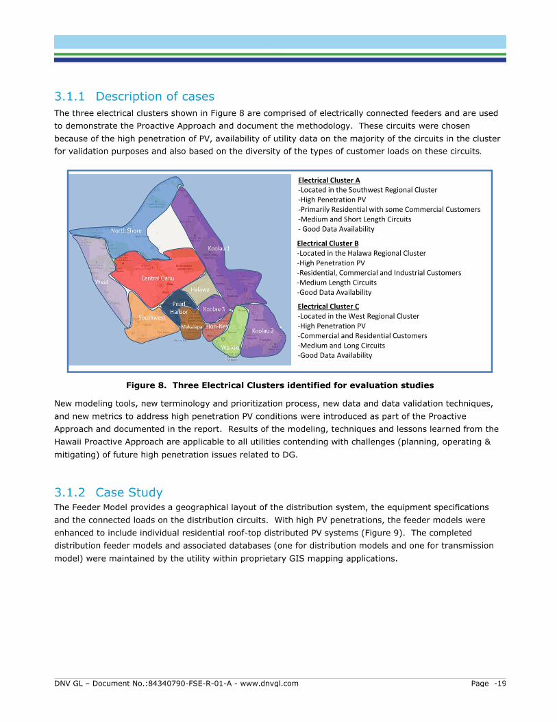
The three electrical clusters shown in Figure 8 are comprised of electrically connected feeders and are used
to demonstrate the Proactive Approach and document the methodology. These circuits were chosen
because of the high penetration of PV, availability of utility data on the majority of the circuits in the cluster
for validation purposes and also based on the diversity of the types of customer loads on these circuits.
Figure 8. Three Electrical Clusters identified for evaluation studies
New modeling tools, new terminology and prioritization process, new data and data validation techniques,
and new metrics to address high penetration PV conditions were introduced as part of the Proactive
Approach and documented in the report. Results of the modeling, techniques and lessons learned from the
Hawaii Proactive Approach are applicable to all utilities contending with challenges (planning, operating &
mitigating) of future high penetration issues related to DG.
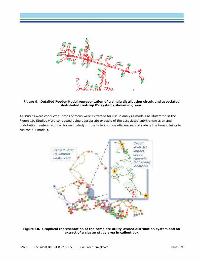
3.1.2 Case Study The Feeder Model provides a geographical layout of the distribution system, the equipment specifications
and the connected loads on the distribution circuits. With high PV penetrations, the feeder models were
enhanced to include individual residential roof-top distributed PV systems (Figure 9). The completed
distribution feeder models and associated databases (one for distribution models and one for transmission
model) were maintained by the utility within proprietary GIS mapping applications.
Electrical Cluster A -Located in the Southwest Regional Cluster -High Penetration PV -Primarily Residential with some Commercial Customers -Medium and Short Length Circuits - Good Data Availability
Electrical Cluster B -Located in the Halawa Regional Cluster -High Penetration PV -Residential, Commercial and Industrial Customers -Medium Length Circuits -Good Data Availability
Electrical Cluster C -Located in the West Regional Cluster -High Penetration PV -Commercial and Residential Customers -Medium and Long Circuits -Good Data Availability
DNV GL – Document No.:84340790-FSE-R-01-A - www.dnvgl.com Page -20
Figure 9. Detailed Feeder Model representation of a single distribution circuit and associated distributed roof-top PV systems shown in green.
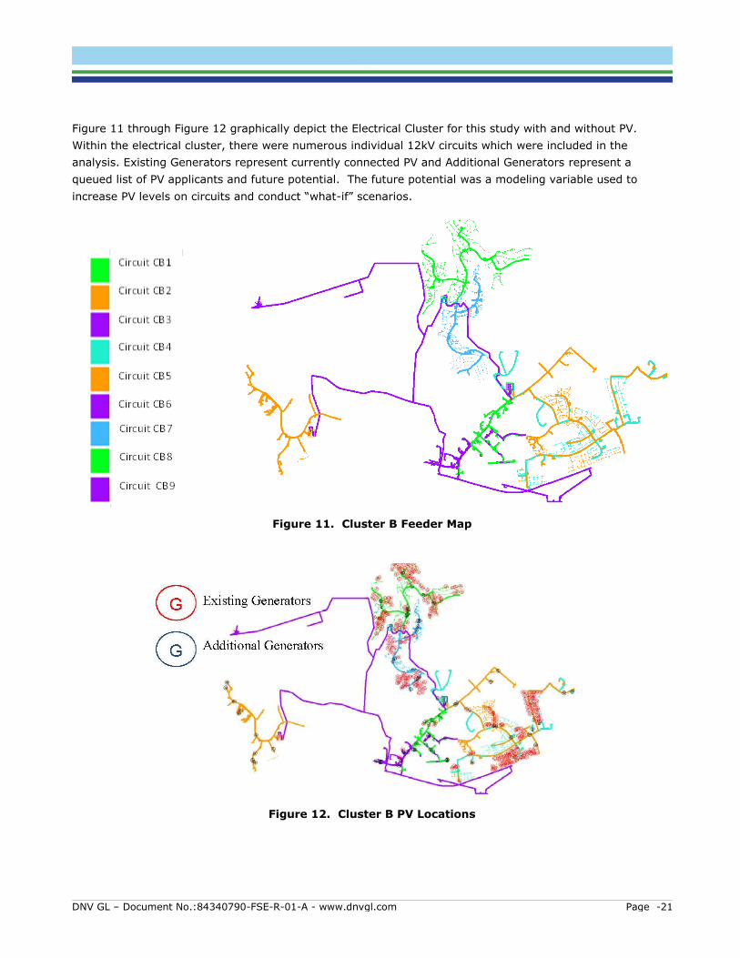
As studies were conducted, areas of focus were extracted for use in analysis models as illustrated in the
Figure 10. Studies were conducted using appropriate extracts of the associated sub-transmission and
distribution feeders required for each study primarily to improve efficiencies and reduce the time it takes to
run the full models.
Figure 10. Graphical representation of the complete utility-owned distribution system and an extract of a cluster study area in callout box
DNV GL – Document No.:84340790-FSE-R-01-A - www.dnvgl.com Page -21
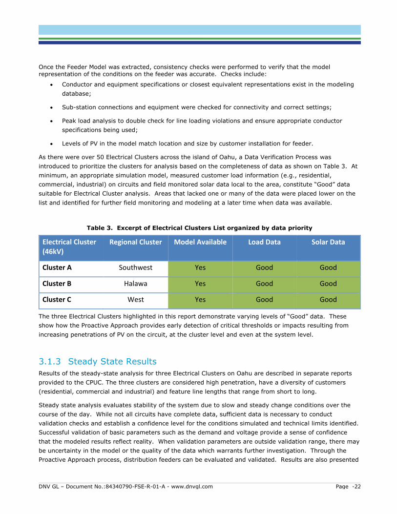
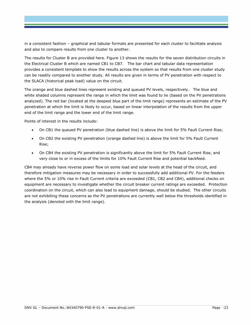
Figure 11 through Figure 12 graphically depict the Electrical Cluster for this study with and without PV.
Within the electrical cluster, there were numerous individual 12kV circuits which were included in the
analysis. Existing Generators represent currently connected PV and Additional Generators represent a
queued list of PV applicants and future potential. The future potential was a modeling variable used to
increase PV levels on circuits and conduct “what-if” scenarios.
Figure 11. Cluster B Feeder Map
Figure 12. Cluster B PV Locations
DNV GL – Document No.:84340790-FSE-R-01-A - www.dnvgl.com Page -22
Once the Feeder Model was extracted, consistency checks were performed to verify that the model representation of the conditions on the feeder was accurate. Checks include:
Conductor and equipment specifications or closest equivalent representations exist in the modeling
database;
Sub-station connections and equipment were checked for connectivity and correct settings;
Peak load analysis to double check for line loading violations and ensure appropriate conductor
specifications being used;
Levels of PV in the model match location and size by customer installation for feeder.
As there were over 50 Electrical Clusters across the island of Oahu, a Data Verification Process was
introduced to prioritize the clusters for analysis based on the completeness of data as shown on Table 3. At
minimum, an appropriate simulation model, measured customer load information (e.g., residential,
commercial, industrial) on circuits and field monitored solar data local to the area, constitute “Good” data
suitable for Electrical Cluster analysis. Areas that lacked one or many of the data were placed lower on the
list and identified for further field monitoring and modeling at a later time when data was available.
Table 3. Excerpt of Electrical Clusters List organized by data priority
Electrical Cluster (46kV)
Regional Cluster Model Available Load Data Solar Data
Cluster A Southwest Yes Good Good
Cluster B Halawa Yes Good Good
Cluster C West Yes Good Good
The three Electrical Clusters highlighted in this report demonstrate varying levels of “Good” data. These
show how the Proactive Approach provides early detection of critical thresholds or impacts resulting from
increasing penetrations of PV on the circuit, at the cluster level and even at the system level.
3.1.3 Steady State Results
Results of the steady-state analysis for three Electrical Clusters on Oahu are described in separate reports
provided to the CPUC. The three clusters are considered high penetration, have a diversity of customers
(residential, commercial and industrial) and feature line lengths that range from short to long.
Steady state analysis evaluates stability of the system due to slow and steady change conditions over the
course of the day. While not all circuits have complete data, sufficient data is necessary to conduct
validation checks and establish a confidence level for the conditions simulated and technical limits identified.
Successful validation of basic parameters such as the demand and voltage provide a sense of confidence
that the modeled results reflect reality. When validation parameters are outside validation range, there may
be uncertainty in the model or the quality of the data which warrants further investigation. Through the
Proactive Approach process, distribution feeders can be evaluated and validated. Results are also presented
DNV GL – Document No.:84340790-FSE-R-01-A - www.dnvgl.com Page -23
in a consistent fashion – graphical and tabular formats are presented for each cluster to facilitate analysis
and also to compare results from one cluster to another.
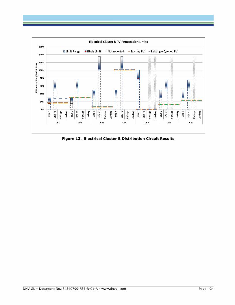
The results for Cluster B are provided here. Figure 13 shows the results for the seven distribution circuits in
the Electrical Cluster B which are named CB1 to CB7. The bar chart and tabular data representation
provides a consistent template to show the results across the system so that results from one cluster study
can be readily compared to another study. All results are given in terms of PV penetration with respect to
the SLACA (historical peak load) value on the circuit.
The orange and blue dashed lines represent existing and queued PV levels, respectively. The blue and
white shaded columns represent the range in which the limit was found to lie (based on the PV penetrations
analyzed). The red bar (located at the deepest blue part of the limit range) represents an estimate of the PV
penetration at which the limit is likely to occur, based on linear interpolation of the results from the upper
end of the limit range and the lower end of the limit range.
Points of interest in the results include:
On CB1 the queued PV penetration (blue dashed line) is above the limit for 5% Fault Current Rise;
On CB2 the existing PV penetration (orange dashed line) is above the limit for 5% Fault Current
Rise;
On CB4 the existing PV penetration is significantly above the limit for 5% Fault Current Rise, and
very close to or in excess of the limits for 10% Fault Current Rise and potential backfeed.
CB4 may already have reverse power flow on some load and solar levels at the head of the circuit, and
therefore mitigation measures may be necessary in order to successfully add additional PV. For the feeders
where the 5% or 10% rise in Fault Current criteria are exceeded (CB1, CB2 and CB4), additional checks on
equipment are necessary to investigate whether the circuit breaker current ratings are exceeded. Protection
coordination on the circuit, which can also lead to equipment damage, should be studied. The other circuits
are not exhibiting these concerns as the PV penetrations are currently well below the thresholds identified in
the analysis (denoted with the limit range).
DNV GL – Document No.:84340790-FSE-R-01-A - www.dnvgl.com Page -24
Figure 13. Electrical Cluster B Distribution Circuit Results
DNV GL – Document No.:84340790-FSE-R-01-A - www.dnvgl.com Page -25
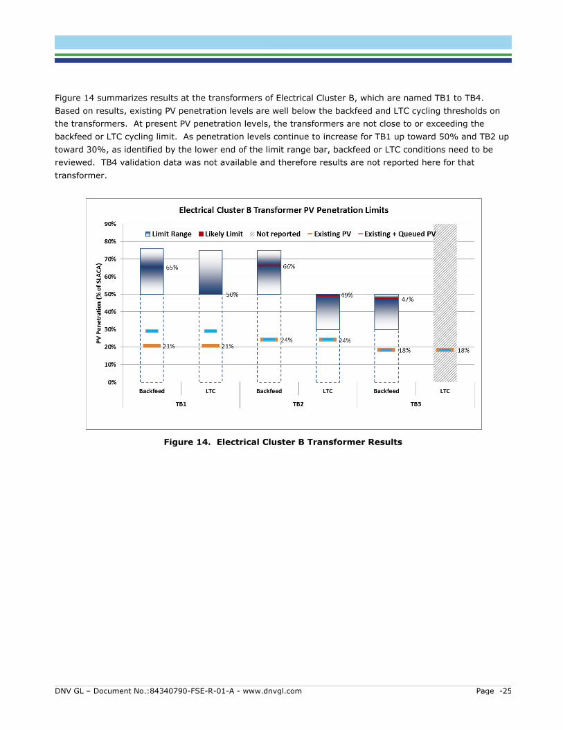
Figure 14 summarizes results at the transformers of Electrical Cluster B, which are named TB1 to TB4.
Based on results, existing PV penetration levels are well below the backfeed and LTC cycling thresholds on
the transformers. At present PV penetration levels, the transformers are not close to or exceeding the
backfeed or LTC cycling limit. As penetration levels continue to increase for TB1 up toward 50% and TB2 up
toward 30%, as identified by the lower end of the limit range bar, backfeed or LTC conditions need to be
reviewed. TB4 validation data was not available and therefore results are not reported here for that
transformer.
Figure 14. Electrical Cluster B Transformer Results
DNV GL – Document No.:84340790-FSE-R-01-A - www.dnvgl.com Page -26
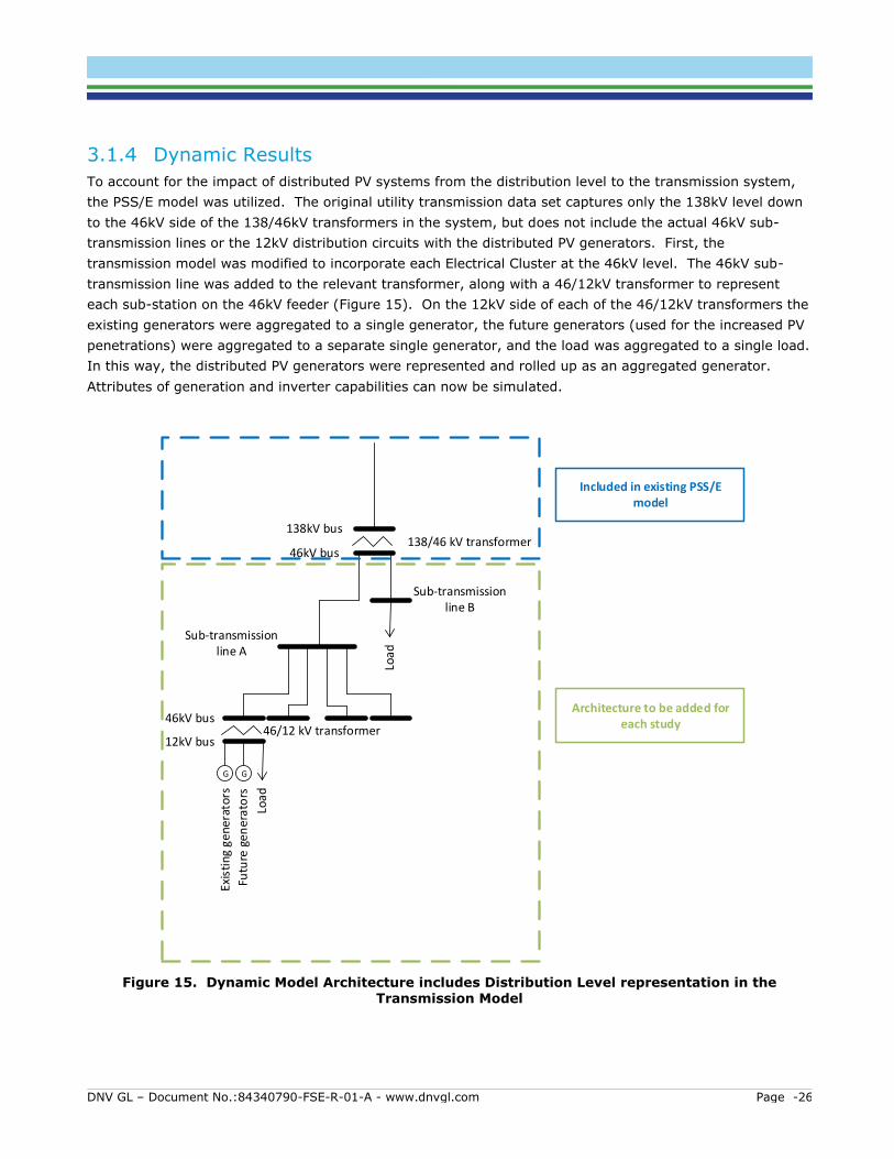
3.1.4 Dynamic Results
To account for the impact of distributed PV systems from the distribution level to the transmission system,
the PSS/E model was utilized. The original utility transmission data set captures only the 138kV level down
to the 46kV side of the 138/46kV transformers in the system, but does not include the actual 46kV sub-
transmission lines or the 12kV distribution circuits with the distributed PV generators. First, the
transmission model was modified to incorporate each Electrical Cluster at the 46kV level. The 46kV sub-
transmission line was added to the relevant transformer, along with a 46/12kV transformer to represent
each sub-station on the 46kV feeder (Figure 15). On the 12kV side of each of the 46/12kV transformers the
existing generators were aggregated to a single generator, the future generators (used for the increased PV
penetrations) were aggregated to a separate single generator, and the load was aggregated to a single load.
In this way, the distributed PV generators were represented and rolled up as an aggregated generator.
Attributes of generation and inverter capabilities can now be simulated.
138/46 kV transformer138kV bus
46kV bus
Sub-transmission line B
Sub-transmission line A
46kV bus
G G
Exis
ting
gen
erat
ors
Futu
re g
ener
ato
rs
Load
Included in existing PSS/E model
Architecture to be added for each study
Load
12kV bus46/12 kV transformer
Figure 15. Dynamic Model Architecture includes Distribution Level representation in the Transmission Model
DNV GL – Document No.:84340790-FSE-R-01-A - www.dnvgl.com Page -27
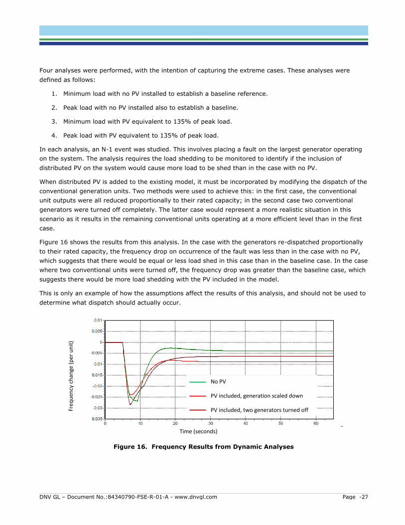
Four analyses were performed, with the intention of capturing the extreme cases. These analyses were
defined as follows:
1. Minimum load with no PV installed to establish a baseline reference.
2. Peak load with no PV installed also to establish a baseline.
3. Minimum load with PV equivalent to 135% of peak load.
4. Peak load with PV equivalent to 135% of peak load.
In each analysis, an N-1 event was studied. This involves placing a fault on the largest generator operating
on the system. The analysis requires the load shedding to be monitored to identify if the inclusion of
distributed PV on the system would cause more load to be shed than in the case with no PV.
When distributed PV is added to the existing model, it must be incorporated by modifying the dispatch of the
conventional generation units. Two methods were used to achieve this: in the first case, the conventional
unit outputs were all reduced proportionally to their rated capacity; in the second case two conventional
generators were turned off completely. The latter case would represent a more realistic situation in this
scenario as it results in the remaining conventional units operating at a more efficient level than in the first
case.
Figure 16 shows the results from this analysis. In the case with the generators re-dispatched proportionally
to their rated capacity, the frequency drop on occurrence of the fault was less than in the case with no PV,
which suggests that there would be equal or less load shed in this case than in the baseline case. In the case
where two conventional units were turned off, the frequency drop was greater than the baseline case, which
suggests there would be more load shedding with the PV included in the model.
This is only an example of how the assumptions affect the results of this analysis, and should not be used to
determine what dispatch should actually occur.
Figure 16. Frequency Results from Dynamic Analyses
Time (seconds)
No PV
PV included, generation scaled down
PV included, two generators turned off Freq
uen
cy c
han
ge (
per
un
it)
DNV GL – Document No.:84340790-FSE-R-01-A - www.dnvgl.com Page -28
Based on this dynamic analysis, distributed generation does have an impact on system performance
especially during contingencies such as the N-1 condition evaluated.
3.1.5 Conclusions and lessons learned
Recommendations for enabling the capabilities of the Proactive Approach include:
Organizational alignment and staff to support and maintain baseline model capabilities;
Process coordination with resource procurement;
Establish regular and timely system-wide reviews to update conditions;
Establish timeframe to conduct baseline planning studies and coordinate with industry;
Revised standards with guidance on procedures for modeling and data analysis;
Support and prioritize ongoing grid and resource monitoring for modeling needs;
Enhance modeling tools with device models to capture future “smart” capabilities;
Maintain this capability through appropriate and consistent workforce training.
Maintaining updated baseline simulation models and routinely conducting analysis based on field data
enables utilities to track changes and assess mitigation strategies in a timely fashion across the overall
electric system instead of one project or circuit at a time. Timely and regular review ensures that baselines
used by transmission and distribution planning adequately keep pace with system and local changes.
The modeling techniques and lessons learned from the Hawaii Proactive Approach are applicable to all
utilities contending with challenges (planning, operating & mitigating) of future high penetration issues
related to DG. As part of the review process for Proactive Approach, industry subject matter experts from
utility and organizations like EPRI provided support for a new process that integrates simulation based
modeling capability and data-driven analysis.
As utilities, Hawaiian Electric Companies are one of the utilities contending with some of the highest levels of
distributed PV penetration and are actively working with other utilities like the Sacramento Municipal Utility
District, and with support from industry, state and federal resources, to devise ways to assess and address
change and enable cost-effective transformation strategies for electric customers. The Proactive Approach
does not solve all the issues but hopefully can provide the beginnings of a consistent framework and
systematic processes to organize data, prioritize through establishing thresholds, perform evaluations with
appropriate models and communicate findings to inform decision-making.
DNV GL – Document No.:84340790-FSE-R-01-A - www.dnvgl.com Page -29
3.2 MECO transmission grid study
The objective of the study on the MECO system was the assessment of the impacts associated with high
penetrations of solar growth on the transmission system in terms of the steady state voltage and thermal
violations. Steady state AC power flow analysis was performed under normal operating and contingency
conditions to identify thermal or voltage violations associated with the future high PV penetration levels in
the MECO transmission system vis-à-vis MECO planning criteria.
3.2.1 Description of cases
For MECO, the study begins at the transmission level and works downward to the distribution level. This is
opposite to the HECO study that works from the distribution level upward to the transmission level.
However, the MECO study continues to follow the Proactive Approach to high penetration analysis of
distributed solar.
The reasons for conducting the high solar penetration study from the transmission perspective for MECO
are:
Transmission problems currently exist due to the installed distributed solar penetrations (32 MW)
Wind generation (72 MW) is located on the transmission grid
o Wind farm #2 has a 11MW 4.4MWh energy storage system that provides ramp rate control
and inertial response.
o Wind farm #3 has a 10MW, 20MWh energy storage system that provides ramp rate control,
frequency regulation outside of the operating dead band and operating reserves based on
system state of charge.
The existence of wind and energy storage on the small MECO system (194 MW) creates unique stability and
reliability issues when studying high penetrations of distributed solar. If wind generation is generating
during the same time periods as solar generation, the net system demand limits the maximum allowable
penetration of solar or causes wind curtailment. The energy storage utilized by wind farm #3 can provide
operating reserves which reduces the need for conventional generation allowing for additional generation to
be accepted from renewable resources.
3.2.2 Case study The scope associated with the steady state study for future solar PV penetration on the MECO transmission
system was defined to address the following:
Develop future solar PV scenarios with increasing PV penetration based on the generation dispatch
priority, must-run conditions for select generation units and minimum spinning reserve criteria.
Assess the impact of the future PV growth on the security of the MECO transmission system from a
steady state standpoint under normal operating and contingency conditions including N-1, G-1, and
loss of combined cycle units.
DNV GL – Document No.:84340790-FSE-R-01-A - www.dnvgl.com Page -30
Determine the maximum amount of solar PV which the MECO transmission system could reliably
accommodate without violating the steady state performance criteria.
Develop the contour maps of the MECO transmission system identifying the regions facing steady
state voltage and thermal violations for future PV scenarios.
3.2.3 Conclusions and lessons learned
Based on the study assumptions documented in previous sections, the following conclusions are
recommended from the results of this steady state analysis of the MECO transmission system to evaluate
the impact of future solar PV growth.
Based on the aforementioned analysis and results, any future PV penetration beyond 37 MW needs
to be examined carefully in the wake of the following:
o Over-voltage violations become severe beyond 30% (37 MW) PV during minimum load and
55% (107 MW) PV during peak load during N-1 contingency operations. Hence, MECO may
need to re-evaluate the operations strategy in terms of capacitor bank switching including
the load thresholds at which the capacitor banks are switched to ensure an acceptable
voltage profile for high PV penetration.
o Operational mitigation actions such as Remedial Actions Plans (RAPs) including capacitor
switching and transformer tap adjustment associated with specific N-1 conditions may need
to be evaluated to limit over-voltage during high PV penetration scenarios.
The maximum amount of solar PV which could be dispatched was 62% of the load under minimum
daytime peak load conditions and 76% of the load under maximum daytime peak load conditions.
Dispatch priorities, must-run conditions for conventional units and available wind generation or
curtailments were the limiting factors for maximum PV penetration.
It is recommended that MECO conduct a statistical analysis on the availability of wind generation
during the minimum and maximum daytime peak loads to determine the probable wind generation
during these time periods. It is also recommended that MECO conduct a study on the correlation of
wind and solar generation over 3-4 years of hourly or sub-hourly load data to determine the
maximum generation of wind and solar over the hourly peak time periods between 10am and 4pm
to determine the amount of wind generation and solar penetration that MECO can absorb.
For daytime minimum load conditions, no thermal or voltage limit violations were observed for
normal operating conditions for all the current and future PV scenarios being considered for study up
to the maximum of 62% of the minimum daytime peak load. For N-1 contingency operations, no
thermal violations were observed for any of the future scenarios however over-voltage violations
were observed across all the current and future PV scenarios.
For maximum daytime peak load conditions, no thermal or voltage limit violations were observed for
normal operating conditions for all the current and future PV scenarios being studied up to the
maximum of 76% of the maximum daytime peak load. For N-1 contingency operations, no thermal
violations were observed however similar to the observations during minimum load conditions, over-

DNV GL – Document No.:84340790-FSE-R-01-A - www.dnvgl.com Page -31
voltage violations were observed across all the future PV scenarios where solar PV penetration
exceeds 25% of the maximum daytime peak load (48 MW).
Over-voltage violations were observed to be the most critical issue for future PV scenarios for both
minimum and maximum daytime peak load conditions from a steady state standpoint. Over-voltage
violations were more severe in minimum daytime load conditions compared to maximum peak load
conditions because of the lighter loading of lines during minimum load conditions.
For study scenarios having more than 30% (37 MW) PV penetration during minimum daytime peak
load and 55% (107 MW) during maximum daytime peak load conditions, more than 15 buses may
have over-voltage violations during N-1 contingency operations.
3.3 Molokai transmission grid study
Molokai has 1.4 MW of existing distributed solar installed and another 1.2 MW of solar in the queue. For
study purposes, Molokai wanted to model 75% of the existing solar (1.05 MW) as generating during the
studied hours. Molokai has a 17% solar penetration. If the 1.2 MW of queued solar becomes commercial,
the Molokai solar penetration increases to 31%. Molokai wanted to determine the total distributed solar that
could be installed.
Since Molokai does not have a transmission system but only a 12kV distribution grid, given its small size, a
distribution integration study was completed. The study approach follows the Proactive Approach
methodology being evaluated under the CPUC CSI RD&D Solicitation 3.
3.3.1 Brief description of Utility
The Island of Molokai is 38 by 10 miles in size at its extreme length and width with a usable land area of 260
square miles. The population of the island is about 7,500 with a maximum electric peak load of 6.3 MW.
Figure 17 shows an aerial map of the island. The Island of Molokai has its own local 12 MW of oil fueled
diesel generation and operations department but the planning is conducted by MECO.
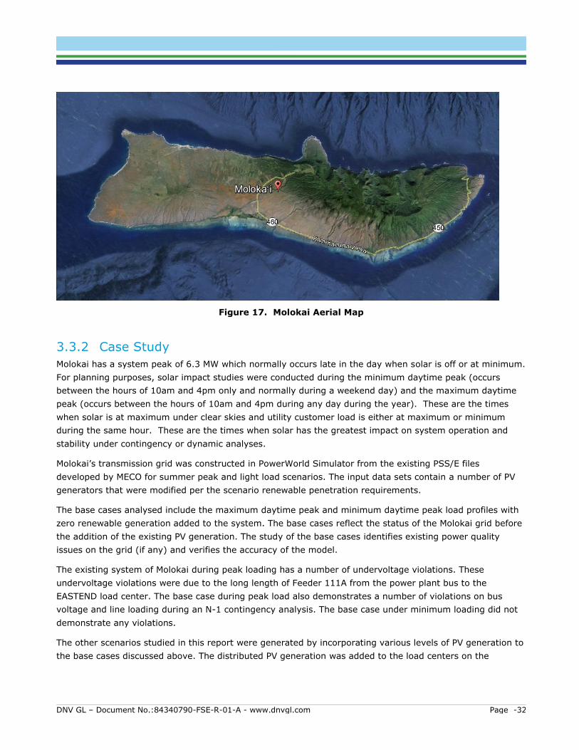
DNV GL – Document No.:84340790-FSE-R-01-A - www.dnvgl.com Page -32
Figure 17. Molokai Aerial Map
3.3.2 Case Study
Molokai has a system peak of 6.3 MW which normally occurs late in the day when solar is off or at minimum.
For planning purposes, solar impact studies were conducted during the minimum daytime peak (occurs
between the hours of 10am and 4pm only and normally during a weekend day) and the maximum daytime
peak (occurs between the hours of 10am and 4pm during any day during the year). These are the times
when solar is at maximum under clear skies and utility customer load is either at maximum or minimum
during the same hour. These are the times when solar has the greatest impact on system operation and
stability under contingency or dynamic analyses.
Molokai’s transmission grid was constructed in PowerWorld Simulator from the existing PSS/E files
developed by MECO for summer peak and light load scenarios. The input data sets contain a number of PV
generators that were modified per the scenario renewable penetration requirements.
The base cases analysed include the maximum daytime peak and minimum daytime peak load profiles with
zero renewable generation added to the system. The base cases reflect the status of the Molokai grid before
the addition of the existing PV generation. The study of the base cases identifies existing power quality
issues on the grid (if any) and verifies the accuracy of the model.
The existing system of Molokai during peak loading has a number of undervoltage violations. These
undervoltage violations were due to the long length of Feeder 111A from the power plant bus to the
EASTEND load center. The base case during peak load also demonstrates a number of violations on bus
voltage and line loading during an N-1 contingency analysis. The base case under minimum loading did not
demonstrate any violations.
The other scenarios studied in this report were generated by incorporating various levels of PV generation to
the base cases discussed above. The distributed PV generation was added to the load centers on the
DNV GL – Document No.:84340790-FSE-R-01-A - www.dnvgl.com Page -33
transmisison grid model and analysed for bus voltage, line loading, and back feed violations during normal
operation and all possible N-1 contingencies.
3.3.3 Conclusions and lessons learned
The steady state analysis of the Molokai network during maximum daytime peak and minimum daytime
loading scenarios with various PV penetration levels (0%, 25%, 39%, 60%, 80%, and 100%) results in
identifying the PV penetration level at which technical criteria for line loading, bus voltage, and back feed
were violated.
The majority of violations detected in this analysis consisted of under voltage conditions occurring at the
EASTEND (EE) location during contingency modes.
As a mitigation measure of these violation instances at the far end of Feeder 106 that serves the EASTEND
load centre, it was decided to study the impacts of battery storage in improving the voltage conditions in
that area. This addition resulted in a noticeable improvement in the operating conditions during normal
operation (N-0) contingency. The impacts to the system during N-1 contingencies were less apparent as the
under voltage instances were still prevalent in the EE load centre. The number of violations and the extents
of them however were decreased in comparison to cases analysed without battery storage.
The results of the study of all loading and PV penetration scenarios indicated above show that any PV
penetration beyond 2.7 MW (with battery storage), equivalent to 50% penetration, causes voltage and
loading violations for the system during N-1 contingencies. 2.7 MW of PV generation is more than the
queued PV amount for Molokai. Any higher penetrations of PV in the system require considerable curtailment
of the PV output to maintain system stability.
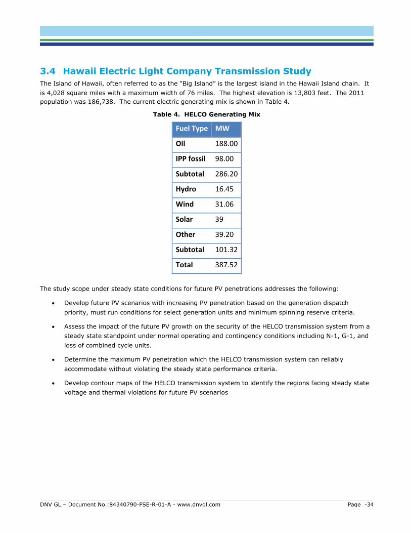
DNV GL – Document No.:84340790-FSE-R-01-A - www.dnvgl.com Page -34
3.4 Hawaii Electric Light Company Transmission Study
The Island of Hawaii, often referred to as the “Big Island” is the largest island in the Hawaii Island chain. It
is 4,028 square miles with a maximum width of 76 miles. The highest elevation is 13,803 feet. The 2011
population was 186,738. The current electric generating mix is shown in Table 4.
Table 4. HELCO Generating Mix
Fuel Type MW
Oil 188.00
IPP fossil 98.00
Subtotal 286.20
Hydro 16.45
Wind 31.06
Solar 39
Other 39.20
Subtotal 101.32
Total 387.52
The study scope under steady state conditions for future PV penetrations addresses the following:
Develop future PV scenarios with increasing PV penetration based on the generation dispatch
priority, must run conditions for select generation units and minimum spinning reserve criteria.
Assess the impact of the future PV growth on the security of the HELCO transmission system from a
steady state standpoint under normal operating and contingency conditions including N-1, G-1, and
loss of combined cycle units.
Determine the maximum PV penetration which the HELCO transmission system can reliably
accommodate without violating the steady state performance criteria.
Develop contour maps of the HELCO transmission system to identify the regions facing steady state
voltage and thermal violations for future PV scenarios
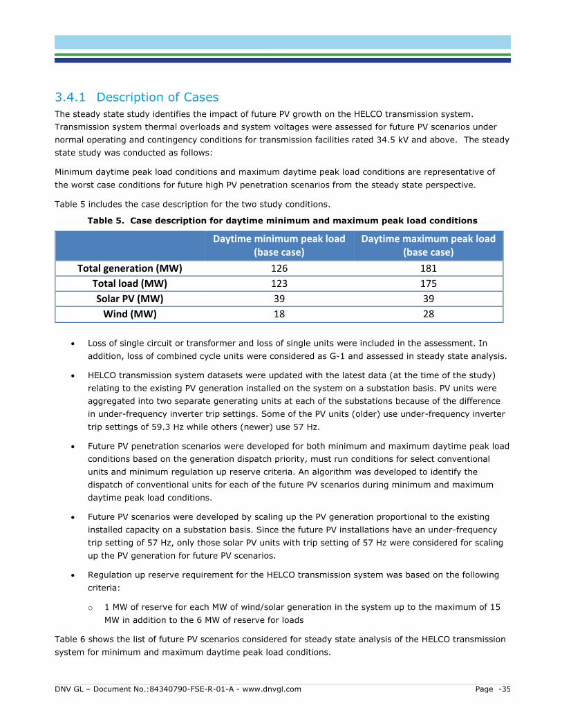
DNV GL – Document No.:84340790-FSE-R-01-A - www.dnvgl.com Page -35
3.4.1 Description of Cases
The steady state study identifies the impact of future PV growth on the HELCO transmission system.
Transmission system thermal overloads and system voltages were assessed for future PV scenarios under
normal operating and contingency conditions for transmission facilities rated 34.5 kV and above. The steady
state study was conducted as follows:
Minimum daytime peak load conditions and maximum daytime peak load conditions are representative of
the worst case conditions for future high PV penetration scenarios from the steady state perspective.
Table 5 includes the case description for the two study conditions.
Table 5. Case description for daytime minimum and maximum peak load conditions
Daytime minimum peak load (base case)
Daytime maximum peak load (base case)
Total generation (MW) 126 181
Total load (MW) 123 175
Solar PV (MW) 39 39
Wind (MW) 18 28
Loss of single circuit or transformer and loss of single units were included in the assessment. In
addition, loss of combined cycle units were considered as G-1 and assessed in steady state analysis.
HELCO transmission system datasets were updated with the latest data (at the time of the study)
relating to the existing PV generation installed on the system on a substation basis. PV units were
aggregated into two separate generating units at each of the substations because of the difference
in under-frequency inverter trip settings. Some of the PV units (older) use under-frequency inverter
trip settings of 59.3 Hz while others (newer) use 57 Hz.
Future PV penetration scenarios were developed for both minimum and maximum daytime peak load
conditions based on the generation dispatch priority, must run conditions for select conventional
units and minimum regulation up reserve criteria. An algorithm was developed to identify the
dispatch of conventional units for each of the future PV scenarios during minimum and maximum
daytime peak load conditions.
Future PV scenarios were developed by scaling up the PV generation proportional to the existing
installed capacity on a substation basis. Since the future PV installations have an under-frequency
trip setting of 57 Hz, only those solar PV units with trip setting of 57 Hz were considered for scaling
up the PV generation for future PV scenarios.
Regulation up reserve requirement for the HELCO transmission system was based on the following
criteria:
o 1 MW of reserve for each MW of wind/solar generation in the system up to the maximum of 15
MW in addition to the 6 MW of reserve for loads
Table 6 shows the list of future PV scenarios considered for steady state analysis of the HELCO transmission
system for minimum and maximum daytime peak load conditions.
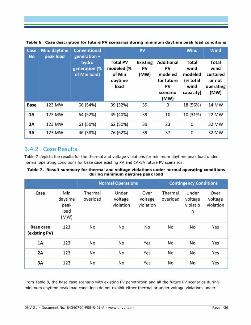
DNV GL – Document No.:84340790-FSE-R-01-A - www.dnvgl.com Page -36
Table 6. Case description for future PV scenarios during minimum daytime peak load conditions
Case No
Min. daytime peak load
Conventional generation +
hydro generation (% of Min load)
PV Wind Wind
Total PV modeled (%
of Min daytime
load
Existing PV
(MW)
Additional PV
modeled for future
PV scenario
(MW)
Total wind
modeled (% total
wind capacity)
Total wind
curtailed or not
operating (MW)
Base 123 MW 66 (54%) 39 (32%) 39 0 18 (56%) 14 MW
1A 123 MW 64 (52%) 49 (40%) 39 10 10 (31%) 22 MW
2A 123 MW 61 (50%) 62 (50%) 39 23 0 32 MW
3A 123 MW 46 (38%) 76 (62%) 39 37 0 32 MW
3.4.2 Case Results
Table 7 depicts the results for the thermal and voltage violations for minimum daytime peak load under
normal operating conditions for base case existing PV and 1A-3A future PV scenarios.
Table 7. Result summary for thermal and voltage violations under normal operating conditions during minimum daytime peak load
Normal Operations Contingency Conditions
Case Min daytime
peak load
(MW)
Thermal overload
Under voltage
violation
Over voltage
violation
Thermal overload
Under voltage violatio
n
Over voltage
violation
Base case (existing PV)
123 No No No No No Yes
1A 123 No No Yes No No Yes
2A 123 No No Yes No No Yes
3A 123 No No Yes No No Yes
From Table 8, the base case scenario with existing PV penetration and all the future PV scenarios during
minimum daytime peak load conditions do not exhibit either thermal or under voltage violations under
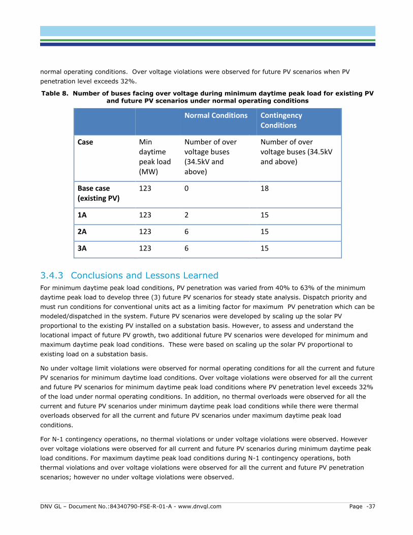
DNV GL – Document No.:84340790-FSE-R-01-A - www.dnvgl.com Page -37
normal operating conditions. Over voltage violations were observed for future PV scenarios when PV
penetration level exceeds 32%.
Table 8. Number of buses facing over voltage during minimum daytime peak load for existing PV and future PV scenarios under normal operating conditions
Normal Conditions Contingency Conditions
Case Min daytime peak load (MW)
Number of over voltage buses (34.5kV and above)
Number of over voltage buses (34.5kV and above)
Base case (existing PV)
123 0 18
1A 123 2 15
2A 123 6 15
3A 123 6 15
3.4.3 Conclusions and Lessons Learned
For minimum daytime peak load conditions, PV penetration was varied from 40% to 63% of the minimum
daytime peak load to develop three (3) future PV scenarios for steady state analysis. Dispatch priority and
must run conditions for conventional units act as a limiting factor for maximum PV penetration which can be
modeled/dispatched in the system. Future PV scenarios were developed by scaling up the solar PV
proportional to the existing PV installed on a substation basis. However, to assess and understand the
locational impact of future PV growth, two additional future PV scenarios were developed for minimum and
maximum daytime peak load conditions. These were based on scaling up the solar PV proportional to
existing load on a substation basis.
No under voltage limit violations were observed for normal operating conditions for all the current and future
PV scenarios for minimum daytime load conditions. Over voltage violations were observed for all the current
and future PV scenarios for minimum daytime peak load conditions where PV penetration level exceeds 32%
of the load under normal operating conditions. In addition, no thermal overloads were observed for all the
current and future PV scenarios under minimum daytime peak load conditions while there were thermal
overloads observed for all the current and future PV scenarios under maximum daytime peak load
conditions.
For N-1 contingency operations, no thermal violations or under voltage violations were observed. However
over voltage violations were observed for all current and future PV scenarios during minimum daytime peak
load conditions. For maximum daytime peak load conditions during N-1 contingency operations, both
thermal violations and over voltage violations were observed for all the current and future PV penetration
scenarios; however no under voltage violations were observed.
DNV GL – Document No.:84340790-FSE-R-01-A - www.dnvgl.com Page -38
Over voltage violations were observed to be the most critical issue for future PV scenarios for both minimum
and maximum daytime peak load conditions. Over voltage violations were more severe during minimum
daytime peak load conditions compared to maximum daytime peak load conditions due to lighter loading of
lines.
3.5 Sacramento Municipal Utility District (SMUD) cases
3.5.1 Task 1 EG Regional Distribution Study
A total of 11 distribution feeders were studied in the SMUD service area under the CPUC CSI RD&D
Solicitation 1. Several of these feeders were located in the EG service area being analyzed in this study and
were projected to have stability issues due to projected solar development or current solar installations.
Since the EG service area consists of over 69 distribution feeders, projected additional distribution solar
installations and 90 MW of central solar installations, the EG area was selected for more detailed solar
penetration studies. The objective of these studies was to use the Proactive Approach identify potential
voltage and thermal loading violations due to the existing and planned solar installations.
3.5.2 Case study
The Synergi data sets for Banks 1 and 2 were used to study the potential impacts on each distribution
feeder connected to the substation transformer but only Bank 1 is discussed below. All of the feeders
connected to each substation transformer were studied as one system to find the point at which backfeed or
voltage violations occur.
The analysis requires several combinations of load profile, PV penetration and PV output in order to model
the full range of scenarios. Each combination constitutes one ‘case’ with each case having 24 load flow
analyses conducted in Synergi. This represents a 6-hour period from 10am to 4pm split into 15-minute
intervals. For each analysis, results were extracted for:
Maximum line loading
Minimum voltage
Maximum voltage
Feeder demand
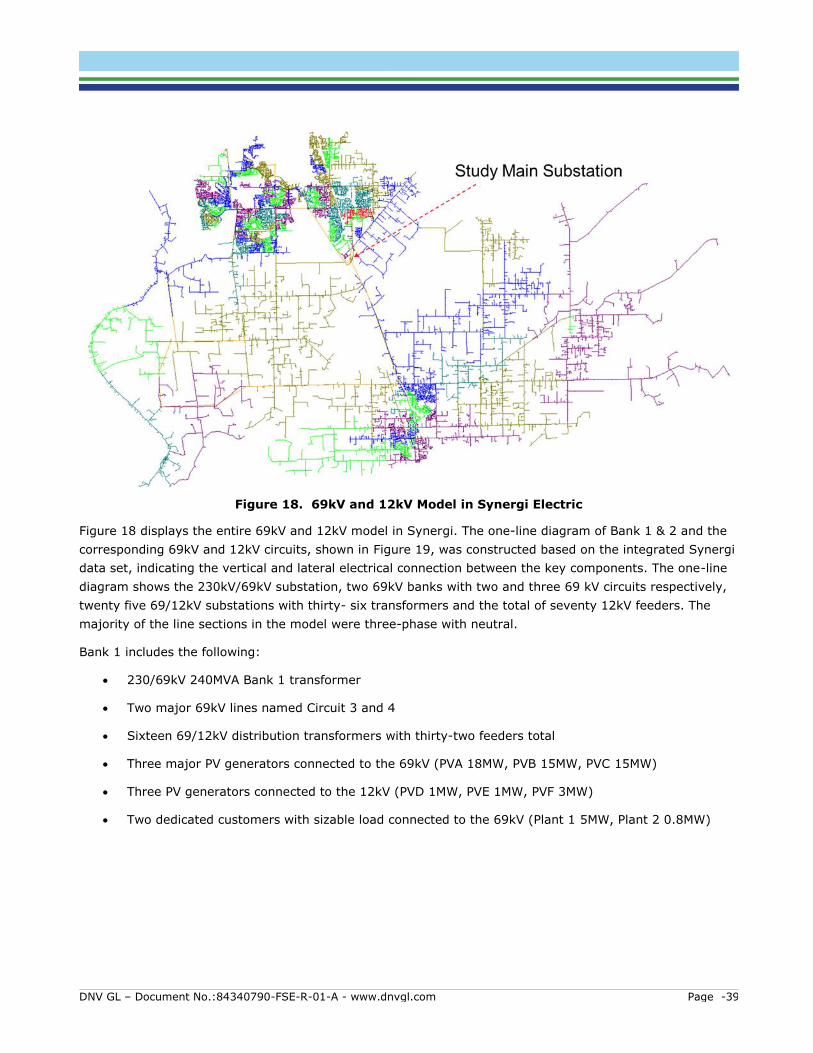
DNV GL – Document No.:84340790-FSE-R-01-A - www.dnvgl.com Page -39
Figure 18. 69kV and 12kV Model in Synergi Electric
Figure 18 displays the entire 69kV and 12kV model in Synergi. The one-line diagram of Bank 1 & 2 and the
corresponding 69kV and 12kV circuits, shown in Figure 19, was constructed based on the integrated Synergi
data set, indicating the vertical and lateral electrical connection between the key components. The one-line
diagram shows the 230kV/69kV substation, two 69kV banks with two and three 69 kV circuits respectively,
twenty five 69/12kV substations with thirty- six transformers and the total of seventy 12kV feeders. The
majority of the line sections in the model were three-phase with neutral.
Bank 1 includes the following:
230/69kV 240MVA Bank 1 transformer
Two major 69kV lines named Circuit 3 and 4
Sixteen 69/12kV distribution transformers with thirty-two feeders total
Three major PV generators connected to the 69kV (PVA 18MW, PVB 15MW, PVC 15MW)
Three PV generators connected to the 12kV (PVD 1MW, PVE 1MW, PVF 3MW)
Two dedicated customers with sizable load connected to the 69kV (Plant 1 5MW, Plant 2 0.8MW)
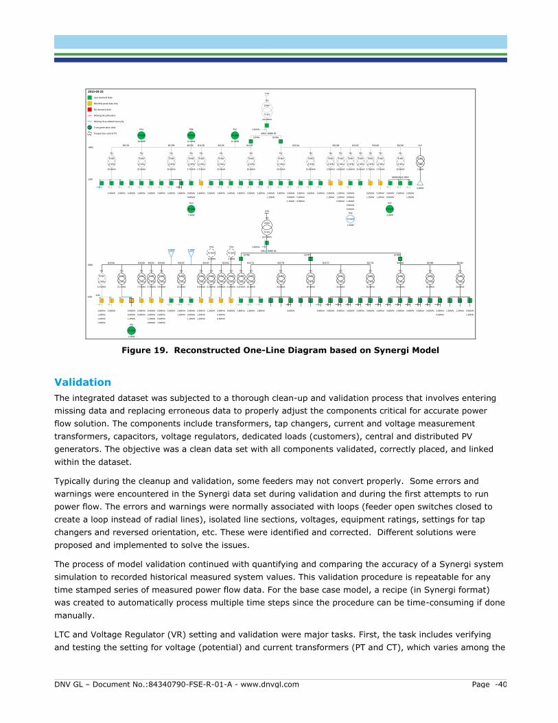
DNV GL – Document No.:84340790-FSE-R-01-A - www.dnvgl.com Page -40
B1C3F
12kV #1
MARENGO SPRR
69kV
CKT#3 CKT#4
69kV BANK #1
#2 #3 #4 #5 #6
B1C3A B1C3B
#1 #2
B1C3C B1C3D B1C3E B1C4A
#1 #1 #1 #2 #3 #1 #2 #3 #1 #2 #3 #4 #5 #6
B1C4B
#1 #2 #2 #3
B1C4C B1C4D B1C4E
#1 #2 #1 #2 #3#3
PV GEN
PVF
3.0MW
PV GEN
PVD
1.0MW
PV GEN
PVB
15.0MW
E
PV GEN
PVC
15.0MW
PV GEN
PVA
18.0MW
70.6kV
12.47kV
20.0MVA
TX1
70.6kV
12.47kV
20.0MVA
70.6kV
12.47kV
20.0MVA
TX1
70.6kV
12.47kV
3.75MVA
TX1
70.6kV
12.47kV
3.75MVA
TX1
70.6kV
12.47kV
20.0MVA
TX1
70.6kV
12.47kV
20.0MVA
TX1
70.6kV
12.47kV
20.0MVA
TX1
70.6kV
12.47kV
20.00MVA
TX2
70.6kV
12.47kV
3.92MVA
TX1
70.6kV
12.47kV
4.69MVA
TX2
70.6kV
12.47kV
6.25MVA
TX1
70.6kV
12.47kV
20.0MVA
TX2
70.6kV
12.47kV
3.75MVA
TX1
70.6kV
12.47kV
3.75MVA
TX2
70.6kV
12.47kV
20.0MVA
TX1
5sec demand data
Monthly peak data only
No demand data
230kV
73.5kV
140.0MVA
TX1
3.6MVAr 3.6MVAr 3.6MVAr3.6MVAr 3.6MVAr 3.6MVAr 3.6MVAr 3.6MVAr 3.6MVAr 3.6MVAr 3.6MVAr 3.6MVAr 3.6MVAr 3.6MVAr 3.6MVAr 3.6MVAr 3.6MVAr 3.6MVAr 3.6MVAr 3.6MVAr0.6MVAr 0.6MVAr3.6MVAr 1.2MVAr 3.6MVAr3.6MVAr 3.6MVAr 0.6MVAr
0.6MVAr
0.6MVAr
1.2MVAr 0.6MVAr
1.2MVAr
0.6MVAr
0.6MVAr
1.2MVAr 1.2MVAr
0.6MVAr
0.6MVAr
1.2MVAr
0.6MVAr
0.6MVAr
1.2MVAr1.2MVAr 1.2MVAr 0.6MVAr
3.6MVAr
124V
12kV
CKT#7CKT#6
69kV
B2C6A B2C6B B2C6C B2C6D B2C6E B2C6F B2C6G B2C7A B2C7B B2C7C
#1 #2 #3 #1 #1 #1 #1 #2 #3 #1 #2 #1 #2 #1 #2 #3 #1 #2 #3 #1 #2 #3
70.6kV
12.47kV
12.5MVA
TX2
BANK #2
PV GEN
PVI
3.0MW
PV GEN
PVG
30.0MW
PV GEN
PVH
4.0MW
#4
70.6kV
12.47kV
6.25MVA
TX1
70.6kV
12.47kV
3.75MVA
TX1
70.6kV
12.47kV
3.75MVA
TX1
70.6kV
12.47kV
3.92MVA
TX1
70.6kV
12.47kV
20.0MVA
TX1
70.6kV
12.47kV
6.25MVA
TX1
70.6kV
12.47kV
6.25MVA
TX2
70.6kV
12.47kV
4.69MVA
TX1
70.6kV
12.47kV
6.25MVA
TX2
70.6kV
12.47kV
20.0MVA
TX1
70.6kV
12.47kV
20.0MVA
TX1
70.6kV
12.47kV
20.0MVA
TX1
70.6kV
12.47kV
20.0MVA
TX2
12kV
69kV
230kV
73.5kV
224.0MVA
TX2
3.6MVAr 3.6MVAr 0.6MVAr 0.6MVAr 0.6MVAr 3.6MVAr 3.6MVAr 3.6MVAr 1.8MVAr 1.8MVAr 1.8MVAr1.2MVAr 0.6MVAr 0.6MVAr 3.6MVAr
1.2MVAr
1.2MVAr
1.2MVAr
0.6MVAr
0.6MVAr
1.2MVAr
0.6MVAr 0.6MVAr
1.2MVAr
0.6MVAr
0.6MVAr
0.6MVAr
1.2MVAr
1.2MVAr 0.6MVAr
1.2MVAr
0.3MVAr
1.2MVAr
1.2MVAr
0.6MVAr
0.6MVAr
124V
B2C7D B2C8B B2C8C
#1 #2 #3 #1 #2 #3 #1 #2 #3 #1 #2 #3
70.6kV
12.47kV
20.0MVA
TX1
70.6kV
12.47kV
20.0MVA
TX1
70.6kV
12.47kV
20.0MVA
TX1
70.6kV
12.47kV
20.0MVA
TX1
3.6MVAr 3.6MVAr 3.6MVAr 3.6MVAr 3.6MVAr 3.6MVAr 3.6MVAr 3.6MVAr 3.6MVAr 1.2MVAr 1.2MVAr 0.6MVAr
0.6MVAr 1.2MVAr
#4 #5 #6
Missing lines/feeders
Missing lines added manually
Prospective central PVPV GEN
CKT#8
5 sec generation dataPV
GEN
3.6MVAr
B2C8A
3.6MVAr
3.6MVAr 3.6MVAr 3.6MVAr
2013-03-22
TX2
PV GEN
PVE
1.0MW
3.6MVAr
6.1MW9.6MW
70.6kV
0.48kV
1.0MW
L13
0.8MW
70.6kV
12.47kV
TX1
6.25MVA
Figure 19. Reconstructed One-Line Diagram based on Synergi Model
Validation
The integrated dataset was subjected to a thorough clean-up and validation process that involves entering
missing data and replacing erroneous data to properly adjust the components critical for accurate power
flow solution. The components include transformers, tap changers, current and voltage measurement
transformers, capacitors, voltage regulators, dedicated loads (customers), central and distributed PV
generators. The objective was a clean data set with all components validated, correctly placed, and linked
within the dataset.
Typically during the cleanup and validation, some feeders may not convert properly. Some errors and
warnings were encountered in the Synergi data set during validation and during the first attempts to run
power flow. The errors and warnings were normally associated with loops (feeder open switches closed to
create a loop instead of radial lines), isolated line sections, voltages, equipment ratings, settings for tap
changers and reversed orientation, etc. These were identified and corrected. Different solutions were
proposed and implemented to solve the issues.
The process of model validation continued with quantifying and comparing the accuracy of a Synergi system
simulation to recorded historical measured system values. This validation procedure is repeatable for any
time stamped series of measured power flow data. For the base case model, a recipe (in Synergi format)
was created to automatically process multiple time steps since the procedure can be time-consuming if done
manually.
LTC and Voltage Regulator (VR) setting and validation were major tasks. First, the task includes verifying
and testing the setting for voltage (potential) and current transformers (PT and CT), which varies among the
DNV GL – Document No.:84340790-FSE-R-01-A - www.dnvgl.com Page -41
devices in the field. The PT setting was determined to be 100:1 line-line with 12kV as designated nominal kV
for the distribution circuit. The CT settings were directly dependent on the transformer MVA rating that can
span a wide range of ratings from 1200:5 to 100:5. Second, the task involves confirming the voltage set-
point, which varies between the feeders (123V to 124V). Finally, the remaining parameters for Line Drop
Compensation: R and X compensation values in the measurement circuit and bandwidth were confirmed and
validated to ensure a stable, reliable response and prevent frequent tap position changes (R=3, X=0,
BW=3).
Capacitor settings and remote vs. local control were discussed to accurately estimate the past response as
well as simulated responses to new scenario cases. Modeling capacitor controls, particularly for capacitors in
the field, were challenging as each capacitor was individually tuned for the specific local conditions.
Issues may be encountered when reviewing large volumes of recorded power demand and generation data.
The days with highly fluctuating irradiance and PV output may be excluded from analysis because such data
may be considered potentially unreliable, if the occurrence was very infrequent or considered too extreme
(which could be caused by non-irradiance-based issues).
Conclusions and Lessons Learned
The CSI3 Proactive Approach was followed for the solar penetration analysis of the EG grid. With SMUD
staff being an active user of the Synergi Electric distribution planning software , the validation and
verification of the input data was completed more easily and quickly than normal. Even though SMUD staff
were active users, additional data was needed for solar penetration studies that were not necessarily used
for most common feeder studies. The results provide SMUD with some potential levels of solar penetrations
per feeder and on the substation transformer and other areas needing further studies.
Synergi was able to model the five 69 kV transmission lines and the sixty-nine distribution lines and
all of the associated loads, capacitor banks, solar installations and line configurations.
Not all feeders have consistent data in the same format. Some have one second data, others
hourly, monthly or no data. However, with the large number of feeders, feeder profiles can be
developed to conduct a high solar penetration study. This data variability demonstrates the need for
a utility to plan ahead for the installation of data recorders to gather consistent, reliable data for
these types of studies.
The location of the distributed solar installations whether at the beginning or end of the feeder
impact the voltage profiles across the feeder.
The location and operation of line capacitors and line regulators has an adverse impact on voltages
and line loadings under high solar penetrations. The utility may need to conduct a detailed
coordination study to determine the relocation and operation of these devices.
The setting of the time delays of substation transformer LTC in conjunction with high solar
penetrations can create short periods of high or low voltages on line sections of feeders. If the time
delays between tap movements were short, then there could be excessive LTC operations and
varying feeder voltages. If the time delays were long, there could be low or high line section
voltages that exceed standard limits.
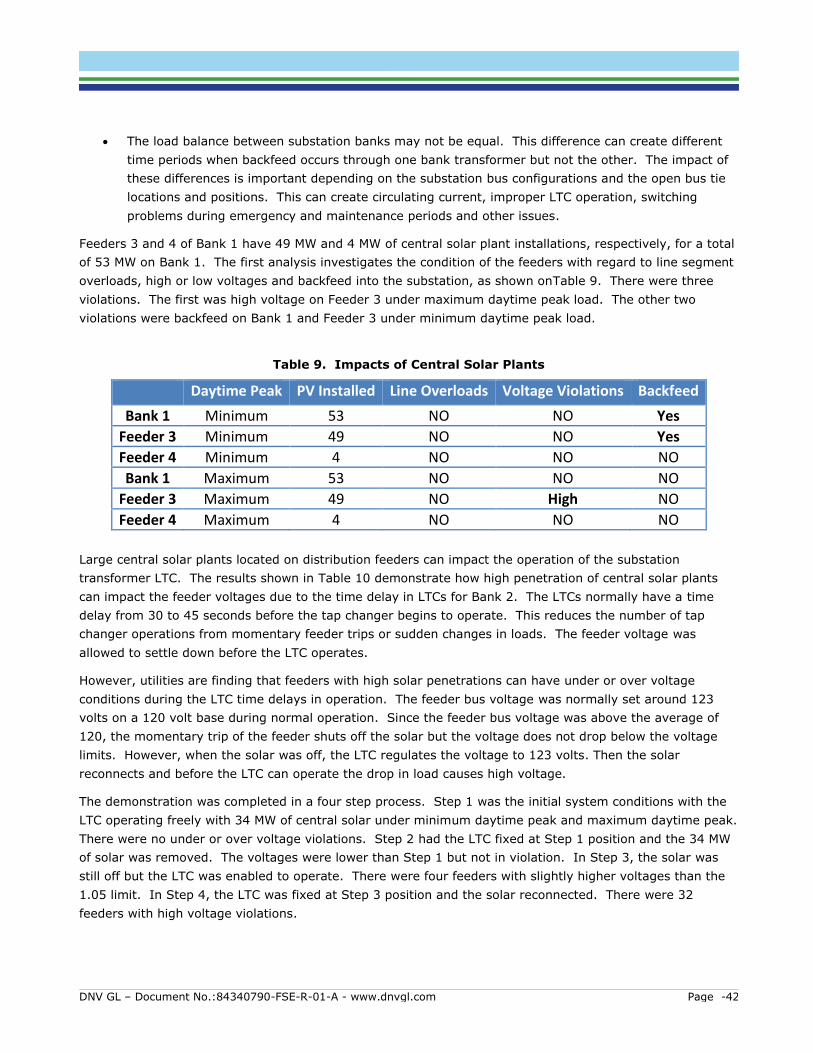
DNV GL – Document No.:84340790-FSE-R-01-A - www.dnvgl.com Page -42
The load balance between substation banks may not be equal. This difference can create different
time periods when backfeed occurs through one bank transformer but not the other. The impact of
these differences is important depending on the substation bus configurations and the open bus tie
locations and positions. This can create circulating current, improper LTC operation, switching
problems during emergency and maintenance periods and other issues.
Feeders 3 and 4 of Bank 1 have 49 MW and 4 MW of central solar plant installations, respectively, for a total
of 53 MW on Bank 1. The first analysis investigates the condition of the feeders with regard to line segment
overloads, high or low voltages and backfeed into the substation, as shown onTable 9. There were three
violations. The first was high voltage on Feeder 3 under maximum daytime peak load. The other two
violations were backfeed on Bank 1 and Feeder 3 under minimum daytime peak load.
Table 9. Impacts of Central Solar Plants
Daytime Peak PV Installed Line Overloads Voltage Violations Backfeed
Bank 1 Minimum 53 NO NO Yes
Feeder 3 Minimum 49 NO NO Yes
Feeder 4 Minimum 4 NO NO NO
Bank 1 Maximum 53 NO NO NO
Feeder 3 Maximum 49 NO High NO
Feeder 4 Maximum 4 NO NO NO
Large central solar plants located on distribution feeders can impact the operation of the substation
transformer LTC. The results shown in Table 10 demonstrate how high penetration of central solar plants
can impact the feeder voltages due to the time delay in LTCs for Bank 2. The LTCs normally have a time
delay from 30 to 45 seconds before the tap changer begins to operate. This reduces the number of tap
changer operations from momentary feeder trips or sudden changes in loads. The feeder voltage was
allowed to settle down before the LTC operates.
However, utilities are finding that feeders with high solar penetrations can have under or over voltage
conditions during the LTC time delays in operation. The feeder bus voltage was normally set around 123
volts on a 120 volt base during normal operation. Since the feeder bus voltage was above the average of
120, the momentary trip of the feeder shuts off the solar but the voltage does not drop below the voltage
limits. However, when the solar was off, the LTC regulates the voltage to 123 volts. Then the solar
reconnects and before the LTC can operate the drop in load causes high voltage.
The demonstration was completed in a four step process. Step 1 was the initial system conditions with the
LTC operating freely with 34 MW of central solar under minimum daytime peak and maximum daytime peak.
There were no under or over voltage violations. Step 2 had the LTC fixed at Step 1 position and the 34 MW
of solar was removed. The voltages were lower than Step 1 but not in violation. In Step 3, the solar was
still off but the LTC was enabled to operate. There were four feeders with slightly higher voltages than the
1.05 limit. In Step 4, the LTC was fixed at Step 3 position and the solar reconnected. There were 32
feeders with high voltage violations.
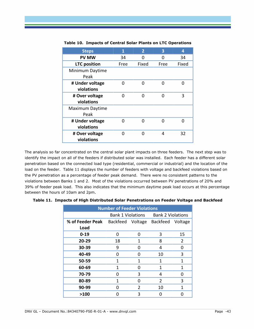
DNV GL – Document No.:84340790-FSE-R-01-A - www.dnvgl.com Page -43
Table 10. Impacts of Central Solar Plants on LTC Operations
Steps 1 2 3 4
PV MW 34 0 0 34
LTC position Free Fixed Free Fixed
Minimum Daytime Peak
# Under voltage violations
0 0 0 0
# Over voltage violations
0 0 0 3
Maximum Daytime Peak
# Under voltage violations
0 0 0 0
# Over voltage violations
0 0 4 32
The analysis so far concentrated on the central solar plant impacts on three feeders. The next step was to
identify the impact on all of the feeders if distributed solar was installed. Each feeder has a different solar
penetration based on the connected load type (residential, commercial or industrial) and the location of the
load on the feeder. Table 11 displays the number of feeders with voltage and backfeed violations based on
the PV penetration as a percentage of feeder peak demand. There were no consistent patterns to the
violations between Banks 1 and 2. Most of the violations occurred between PV penetrations of 20% and
39% of feeder peak load. This also indicates that the minimum daytime peak load occurs at this percentage
between the hours of 10am and 2pm.
Table 11. Impacts of High Distributed Solar Penetrations on Feeder Voltage and Backfeed
Number of Feeder Violations
Bank 1 Violations Bank 2 Violations
% of Feeder Peak Load
Backfeed Voltage Backfeed Voltage
0-19 0 0 3 15
20-29 18 1 8 2
30-39 9 0 4 0
40-49 0 0 10 3
50-59 1 1 1 1
60-69 1 0 1 1
70-79 0 3 4 0
80-89 1 0 2 3
90-99 0 2 10 1
>100 0 3 0 0
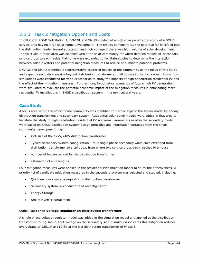
DNV GL – Document No.:84340790-FSE-R-01-A - www.dnvgl.com Page -44
3.5.3 Task 2 Mitigation Options and Costs
In CPUC CSI RD&D Solicitation 1, DNV GL and SMUD conducted a high solar penetration study of a SMUD
service area having large solar home development. The results demonstrated the potential for backfeed into
the distribution feeder toward substation and high voltage if there was high volume of solar development.
In this study, a focus area was selected within the solar community for which detailed models of secondary
service drops to each residential home were expanded to facilitate studies to determine the interaction
between solar inverters and potential mitigation measures to reduce or eliminate potential problems.
DNV GL and SMUD identified a representative cluster of houses in the community as the focus of this study
and expands secondary service beyond distribution transformers to all houses in the focus area. Power flow
simulations were conducted for various scenarios to study the impacts of high penetration residential PV and
the effect of the mitigation measures. Furthermore, hypothetical scenarios of future high PV penetration
were simulated to evaluate the potential economic impact of the mitigation measures in anticipating more
residential PV installations in SMUD’s distribution system in the next several years.
Case Study
A focus area within the smart home community was identified to further expand the feeder model by adding
distribution transformers and secondary system. Residential solar panel models were added in that area to
facilitate the study of high penetration residential PV scenarios. Parameters used in the secondary model
were based on SMUD distribution system design principles and information extracted from the smart
community development map:
kVA size of the 12kV/240V distribution transformer
Typical secondary system configuration – four single phase secondary wires each extended from
distribution transformer to a split box, from where two service drops each reaches to a house.
number of houses served by the distribution transformer
estimation of wire lengths
Four mitigation measures were applied in the residential PV simulation model to study the effectiveness. A
priority list of candidate mitigation measures in the secondary system was selected and studied, including:
Quick response voltage regulator on distribution transformer
Secondary system re-conductor and reconfiguration
Energy Storage
Smart inverter curtailment
Quick Response Voltage Regulator on distribution transformer
A single phase voltage regulator model was added in the simulation model and applied at the distribution
transformer to regulate output voltage on the secondary side. Simulation indicates this mitigation reduces
overvoltage of 125.1V to 119.6V at the last distribution transformer of Phase B.
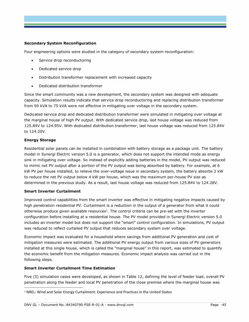
DNV GL – Document No.:84340790-FSE-R-01-A - www.dnvgl.com Page -45
Secondary System Reconfiguration
Four engineering options were studied in the category of secondary system reconfiguration:
Service drop reconductoring
Dedicated service drop
Distribution transformer replacement with increased capacity
Dedicated distribution transformer
Since the smart community was a new development, the secondary system was designed with adequate
capacity. Simulation results indicate that service drop reconductoring and replacing distribution transformer
from 50 kVA to 75 kVA were not effective in mitigating over voltage in the secondary system.
Dedicated service drop and dedicated distribution transformer were simulated in mitigating over voltage at
the marginal house of high PV output. With dedicated service drop, last house voltage was reduced from
125.84V to 124.95V. With dedicated distribution transformer, last house voltage was reduced from 125.84V
to 124.20V.
Energy Storage
Residential solar panels can be installed in combination with battery storage as a package unit. The battery
model in Synergi Electric version 5.0 is a generator, which does not support the intended mode as energy
sink in mitigating over voltage. So instead of explicitly adding batteries in the model, PV output was reduced
to mimic net PV output after a portion of the PV output was being absorbed by battery. For example, at 6
kW PV per house installed, to relieve the over-voltage issue in secondary system, the battery absorbs 2 kW
to reduce the net PV output below 4 kW per house, which was the maximum per-house PV size as
determined in the previous study. As a result, last house voltage was reduced from 125.84V to 124.28V.
Smart Inverter Curtailment
Improved control capabilities from the smart inverter was effective in mitigating negative impacts caused by
high penetration residential PV. Curtailment is a reduction in the output of a generator from what it could
otherwise produce given available resources1. The control criteria can be pre-set with the inverter
configuration before installing at a residential house. The PV model provided in Synergi Electric version 5.0
includes an inverter model but does not support the “smart” control configuration. In simulations, PV output
was reduced to reflect curtailed PV output that reduces secondary system over voltage.
Economic impact was evaluated for a household where savings from additional PV generation and cost of
mitigation measures were estimated. The additional PV energy output from various sizes of PV generators
installed at this single house, which is called the “marginal house” in this report, was estimated to quantify
the economic benefit from the mitigation measures. Economic impact analysis was carried out in the
following steps.
Smart Inverter Curtailment Time Estimation
Five (5) simulation cases were developed, as shown in Table 12, defining the level of feeder load, overall PV
penetration along the feeder and local PV penetration of the close premise where the marginal house was
1 NREL: Wind and Solar Energy Curtailment: Experience and Practices in the United States
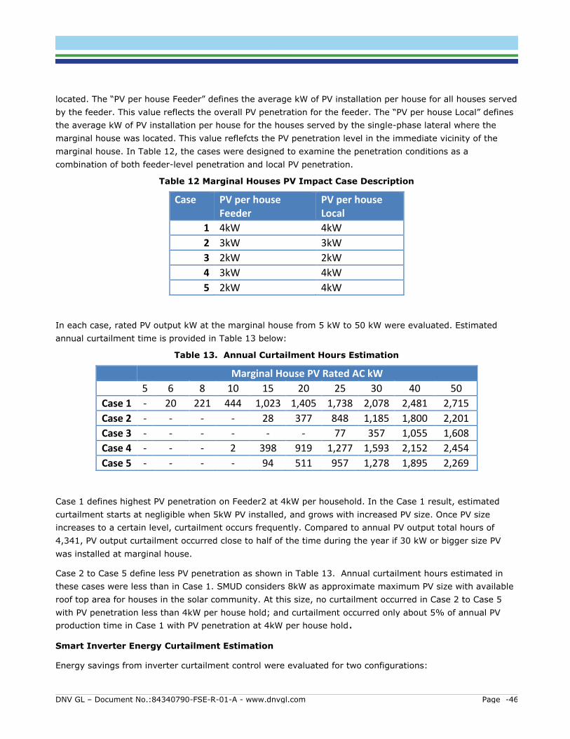
DNV GL – Document No.:84340790-FSE-R-01-A - www.dnvgl.com Page -46
located. The “PV per house Feeder” defines the average kW of PV installation per house for all houses served
by the feeder. This value reflects the overall PV penetration for the feeder. The “PV per house Local” defines
the average kW of PV installation per house for the houses served by the single-phase lateral where the
marginal house was located. This value reflefcts the PV penetration level in the immediate vicinity of the
marginal house. In Table 12, the cases were designed to examine the penetration conditions as a
combination of both feeder-level penetration and local PV penetration.
Table 12 Marginal Houses PV Impact Case Description
Case PV per house Feeder
PV per house Local
1 4kW 4kW
2 3kW 3kW
3 2kW 2kW
4 3kW 4kW
5 2kW 4kW
In each case, rated PV output kW at the marginal house from 5 kW to 50 kW were evaluated. Estimated
annual curtailment time is provided in Table 13 below:
Table 13. Annual Curtailment Hours Estimation
Marginal House PV Rated AC kW
5 6 8 10 15 20 25 30 40 50
Case 1 - 20 221 444 1,023 1,405 1,738 2,078 2,481 2,715
Case 2 - - - - 28 377 848 1,185 1,800 2,201
Case 3 - - - - - - 77 357 1,055 1,608
Case 4 - - - 2 398 919 1,277 1,593 2,152 2,454
Case 5 - - - - 94 511 957 1,278 1,895 2,269
Case 1 defines highest PV penetration on Feeder2 at 4kW per household. In the Case 1 result, estimated
curtailment starts at negligible when 5kW PV installed, and grows with increased PV size. Once PV size
increases to a certain level, curtailment occurs frequently. Compared to annual PV output total hours of
4,341, PV output curtailment occurred close to half of the time during the year if 30 kW or bigger size PV
was installed at marginal house.
Case 2 to Case 5 define less PV penetration as shown in Table 13. Annual curtailment hours estimated in
these cases were less than in Case 1. SMUD considers 8kW as approximate maximum PV size with available
roof top area for houses in the solar community. At this size, no curtailment occurred in Case 2 to Case 5
with PV penetration less than 4kW per house hold; and curtailment occurred only about 5% of annual PV
production time in Case 1 with PV penetration at 4kW per house hold.
Smart Inverter Energy Curtailment Estimation
Energy savings from inverter curtailment control were evaluated for two configurations:
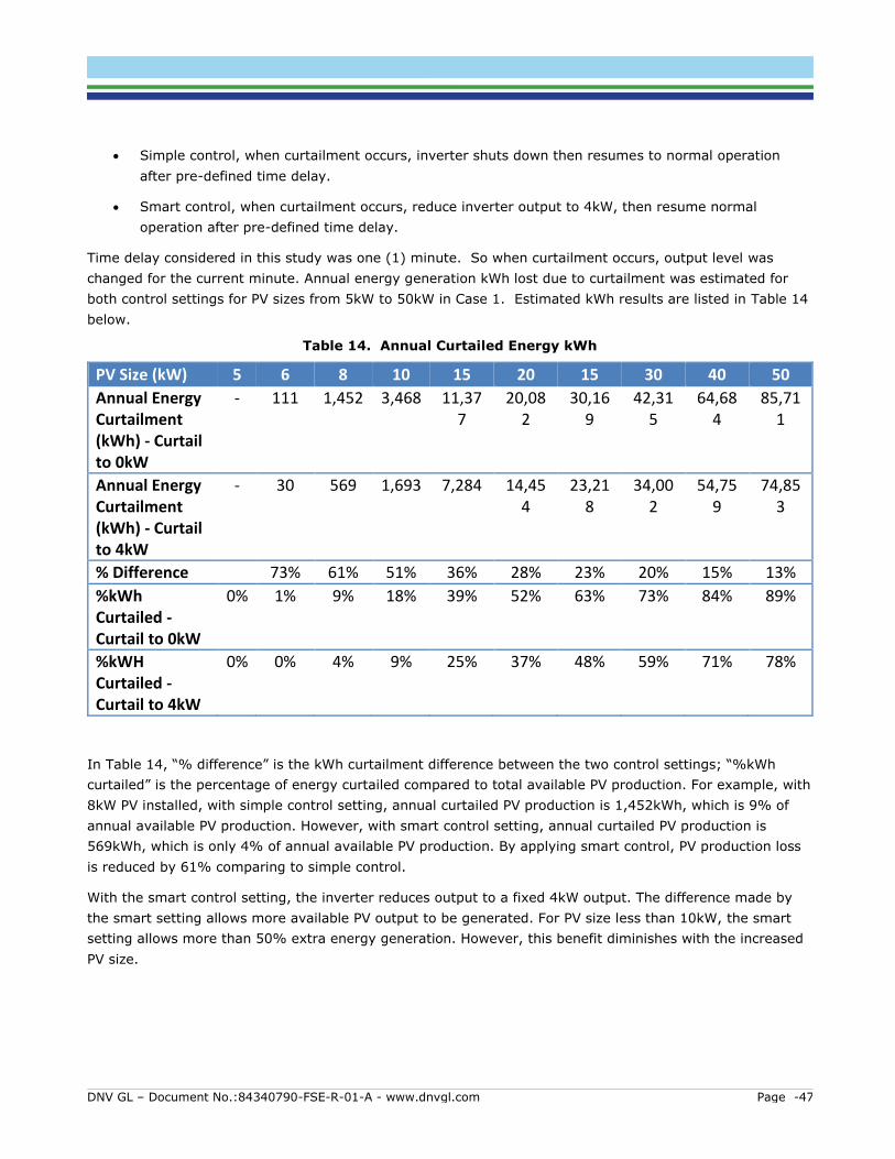
DNV GL – Document No.:84340790-FSE-R-01-A - www.dnvgl.com Page -47
Simple control, when curtailment occurs, inverter shuts down then resumes to normal operation
after pre-defined time delay.
Smart control, when curtailment occurs, reduce inverter output to 4kW, then resume normal
operation after pre-defined time delay.
Time delay considered in this study was one (1) minute. So when curtailment occurs, output level was
changed for the current minute. Annual energy generation kWh lost due to curtailment was estimated for
both control settings for PV sizes from 5kW to 50kW in Case 1. Estimated kWh results are listed in Table 14
below.
Table 14. Annual Curtailed Energy kWh
PV Size (kW) 5 6 8 10 15 20 15 30 40 50
Annual Energy Curtailment (kWh) - Curtail to 0kW
- 111 1,452 3,468 11,377
20,082
30,169
42,315
64,684
85,711
Annual Energy Curtailment (kWh) - Curtail to 4kW
- 30 569 1,693 7,284 14,454
23,218
34,002
54,759
74,853
% Difference 73% 61% 51% 36% 28% 23% 20% 15% 13%
%kWh Curtailed - Curtail to 0kW
0% 1% 9% 18% 39% 52% 63% 73% 84% 89%
%kWH Curtailed - Curtail to 4kW
0% 0% 4% 9% 25% 37% 48% 59% 71% 78%
In Table 14, “% difference” is the kWh curtailment difference between the two control settings; “%kWh
curtailed” is the percentage of energy curtailed compared to total available PV production. For example, with
8kW PV installed, with simple control setting, annual curtailed PV production is 1,452kWh, which is 9% of
annual available PV production. However, with smart control setting, annual curtailed PV production is
569kWh, which is only 4% of annual available PV production. By applying smart control, PV production loss
is reduced by 61% comparing to simple control.
With the smart control setting, the inverter reduces output to a fixed 4kW output. The difference made by
the smart setting allows more available PV output to be generated. For PV size less than 10kW, the smart
setting allows more than 50% extra energy generation. However, this benefit diminishes with the increased
PV size.
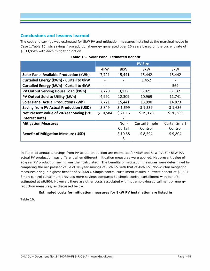
DNV GL – Document No.:84340790-FSE-R-01-A - www.dnvgl.com Page -48
Conclusions and lessons learned
The cost and savings was estimated for 8kW PV and mitigation measures installed at the marginal house in
Case 1.Table 15 lists savings from additional energy generated over 20 years based on the current rate of
$0.11/kWh with each mitigation option.
Table 15. Solar Panel Estimated Benefit
PV Size
4kW 8kW 8kW 8kW
Solar Panel Available Production (kWh) 7,721 15,441 15,442 15,442
Curtailed Energy (kWh) - Curtail to 0kW - - 1,452 -
Curtailed Energy (kWh) - Curtail to 4kW - - - 569
PV Output Serving House Load (kWh) 2,729 3,132 3,021 3,132
PV Output Sold to Utility (kWh) 4,992 12,309 10,969 11,741
Solar Panel Actual Production (kWh) 7,721 15,441 13,990 14,873
Saving from PV Actual Production (USD) $ 849 $ 1,699 $ 1,539 $ 1,636
Net Present Value of 20-Year Saving (5% Interest Rate)
$ 10,584 $ 21,167
$ 19,178 $ 20,389
Mitigation Measures Non-Curtail
Curtail Simple Control
Curtail Smart Control
Benefit of Mitigation Measure (USD) $ 10,583
$ 8,594 $ 9,804
In Table 15 annual $ savings from PV actual production are estimated for 4kW and 8kW PV. For 8kW PV,
actual PV production was different when different mitigation measures were applied. Net present value of
20-year PV production saving was then calculated. The benefits of mitigation measures were determined by
comparing the net present value of 20-year savings of 8kW PV with that of 4kW PV. Non-curtail mitigation
measures bring in highest benefit of $10,683. Simple control curtailment results in lowest benefit of $8,594.
Smart control curtailment provides more savings compared to simple control curtailment with benefit
estimated at $9,804. However, there are other costs associated with not employing curtailment or energy
reduction measures, as discussed below.
Estimated costs for mitigation measures for 8kW PV installation are listed in
Table 16.

DNV GL – Document No.:84340790-FSE-R-01-A - www.dnvgl.com Page -49
Table 16. Estimated Costs of Mitigation Measures for 8kW Solar Panel
Mitigation Measures Estimated Installed Cost
Smart Inverter Curtailment -
4kW Battery Storage at Solar Panel $5,000-$44,000
Single Phase Distribution Transformer with Regulator
$9,700
Dedicated Distribution Transformer $4,200
Dedicated Secondary Cable (100 ft) $2,200
Savings for installing 8kW of solar panels with mitigation measures is between $8,000 and $10,000. Smart
inverter becomes the most cost effective option, followed by dedicated secondary cable and dedicated
transformer. Voltage regulated distribution transformer is close to cost-effective with its current high cost.
Battery storage is still too expensive at its current cost level, however, with the expected price decreasing
trend, battery storage is likely to become a cost effective mitigation option in the future.
DNV GL and SMUD developed a study approach and conducted studies evaluating high penetration
residential PV impacts on the secondary system, effectiveness of mitigation measures and the economic
impacts. The study was conducted by simulating various PV penetration and mitigation scenarios on a SMUD
feeder model using Synergi Electric.
Four mitigation measures on the secondary system were studied, including:
Quick response voltage regulator on distribution transformer
Secondary system reconfiguration
Energy Storage
Smart inverter curtailment
All four approaches can effectively mitigate high voltage in secondary system caused by increased
residential PV penetration.
Evaluation of cost and benefit of these mitigation measures indicates that smart inverter curtailment,
dedicated service drop and dedicated distribution transformer are cost effective mitigation options. However,
cost for energy storage and quick response voltage regulated distribution transformer needs to become
lower to be cost effective.
DNV GL – Document No.:84340790-FSE-R-01-A - www.dnvgl.com Page -50
3.6 City of Roseville
Before Roseville’s participation in the CSI RD&D Solicitaiton 3, Roseville had a moratorium on new
distributed solar installations until a solar penetration study was completed. Roseville participated in this
project to understand the issues from other utilities regarding high solar penetrations. The study centers
on steady-state load flow analyses performed on the Westplan substation for Roseville Electric to identify
potential voltage issues on the Westplan feeders due to increasing distributed solar PV generation. PV
generation is largely a function of incident solar irradiance and can fluctuate widely from minute to minute
as clouds move across the sky. As PV generation varies, so does the net demand at the substation
transformer. Since the on-load tap changer (LTC) is not designed to regulate the feeder or bus voltages
within the short timescales of PV variability, voltage issues may occur at various locations on the feeder that
can be attributed to PV generation. As the amount of PV generation increases on a distribution feeder so
does the risk of voltage issues. Voltage issues that can occur include voltage flicker, device malfunction in
the case of low voltages, and device failure in the case of high voltages. Voltage issues may be temporary
(i.e. relieved after the LTC responds) and may be prolonged if voltages exceed the voltage tolerance of a
device (e.g. a fuse or distribution transformer).
3.6.1 Validation
The customer voltage data measured by Boomerang power quality analyzers in the field contain 240 V
measurements at 1-second resolution for six locations on multiple feeders within the Westplan region. This
data was used with the SCADA data to validate the Westplan model by comparing load flow simulation
voltages to measured voltages at each hour in the minimum demand day.
Model validation was carried out, collecting real-time measurements of power flow (e.g. current, voltage,
real power, and reactive power) at two or more locations within the WESTPLAN system, inputting measured
values appropriately into the Synergi model, and comparing Synergi load flow results to the measured
values. Time-synced measured values input to the Synergi model include: (1) voltage at 60 kV voltage
source (unbalanced three-phase voltages); (2) voltage setting for substation transformer LTCs (unbalanced
three-phase voltages); and (3) distribution feeder demands (unbalanced three-phase currents and power
factor).
This model validation procedure can be repeated for any series of timestamps of measured power flow data.
For the Westplan base case model, the chosen timestamps were the top of each hour throughout either the
peak or minimum demand day. The range of hours simulated was 6AM to 6PM because measured irradiance
and temperature data was limited beyond this range, and there was little to no PV generation outside of this
range. For validation of the Westplan base case model, a recipe (in Synergi format) was created to
automatically process multiple timestamps, since this procedure can be time-consuming if done manually.
DNV GL – Document No.:84340790-FSE-R-01-A - www.dnvgl.com Page -51
3.6.2 Case study
The analyses were performed using the Synergi Electric dataset of Westplan system (hereafter called the
“Westplan model”) provided by Roseville Electric. The Westplan model is an unbalanced, steady-state power
flow model that includes eight 12 kV distribution feeders served by two 60/12kV transformers in the
Westplan substation. The Westplan Buses 1 & 2 are ideal voltage sources with source impedances that
represent the equivalent 60 kV source at the high side of each substation transformer.
The amount of existing PV generation installed in Westplan was considered; and potential future PV
generation was distributed throughout the dataset to simulate future system conditions. The total amount of
potential PV distributed throughout a feeder was increased until voltage issues begin to occur on the feeder,
or until the total amount of PV equals the peak demand measured in 2012 for the feeder, whichever comes
first.
The existing PV generating capacity as of August 2012 was added to the base case Westplan model and held
constant. The instantaneous generation from existing PV generators changes only with time-varying
irradiance. The existing PV locations in the Westplan model were selected using a geographical PV placement
tool developed by DNV GL. The tool uses the street address of each PV site and feeder designation. The
street address was converted to X & Y coordinates in the California Zone II State Plane Coordinate System.
The feeder designation for each PV unit was determined from distribution transformer information. The PV
placement tool matches each PV unit to the closest Synergi node within the correct feeder. The result of the
PV placement tool was that 94% of the existing PV units were placed within 300 feet of the distribution
transformer it was known to be fed by, indicating the PV placement tool was reliably accurate.
There were 829 existing PV units in the Westplan model, with a total kW capacity of 1,653 kW.
Given the limited information as to the sizes and locations of future PV generation, the methodology chosen
to allocate potential PV to the Westplan feeders was as follows. The maximum potential PV capacity on each
distribution feeder was chosen to be 100% of the non-coincident peak load for that feeder. This was a very
high potential PV penetration scenario, but was chosen for this analysis to force system limitations to occur.
For each feeder, the potential PV was distributed proportionally to customer locations across the feeder
according to the connected kVA (c.kVA) value of the customer load as in Equation 1. The c.kVA
approximates the maximum load at the customer location. Note that a customer location in the Westplan
model may be the aggregate of multiple individual customers that were electrically connected in a small area
such as a neighborhood.
𝑘𝑊 𝑜𝑓 𝑝𝑜𝑡𝑒𝑛𝑡𝑖𝑎𝑙 𝑃𝑉 𝑜𝑛 𝑎 𝑠𝑒𝑐𝑡𝑖𝑜𝑛 = (𝑡𝑜𝑡𝑎𝑙 𝑘𝑊 𝑜𝑓 𝑝𝑜𝑡𝑒𝑛𝑡𝑖𝑎𝑙 𝑃𝑉 𝑜𝑛 𝑓𝑒𝑒𝑑𝑒𝑟) ∙(𝑐.𝑘𝑉𝐴 𝑎𝑡 𝑐𝑢𝑠𝑡𝑜𝑚𝑒𝑟 𝑠𝑖𝑡𝑒)
(𝑡𝑜𝑡𝑎𝑙 𝑐.𝑘𝑉𝐴 𝑜𝑛 𝑓𝑒𝑒𝑑𝑒𝑟) (1)
To stay consistent with the PV modeling of the existing feeder, both existing and potential PV generations
were added as aggregate PV generators to the future build out locations. The size of the existing PV
generator on the future build out of each feeder was equivalent to a certain percentage of the future build
out spot load. The potential PV generator was increased up to 100% of the future build out spot load. The
One-Minute PV Ramp Analysis considers PV generation ramping both up and down within one minute. The
PV generation ramps chosen were as follows:
1. PV ramp down from 100% output to 30% output
2. PV ramp down from 100% output to 20% output
DNV GL – Document No.:84340790-FSE-R-01-A - www.dnvgl.com Page -52
3. PV ramp down from 100% output to 0% output
4. PV ramp up from 30% output to 100% output
5. PV ramp up from 20% output to 100% output
6. PV ramp up from 0% output to 100% output
PV ramps to and from 30% output approximate a large change in PV generation due to a change in solar
irradiance that is likely to occur frequently. PV ramps to and from 20% output approximate a large change
in PV generation due to a change in solar irradiance that is likely to occur less frequently. PV ramps from
100% to 0% output approximate a large change in PV generation due to PV tripping off-line due to a
substation, bus or transmission trip or outage. This occurs because distributed PV generators are required to
disconnect at 59.3 Hz to conform to IEEE Standard 1547. PV ramps from 0% to 100% output approximate a
large change in PV generation due to PV reconnecting after such an outage event. This can occur because
distributed PV generators are required by UL 1741 to wait to reconnect until at least five minutes after
system frequency and voltage return to normal. During this five minute period, the LTC has sufficient time
to adjust its tap position to account for the lack of PV generation.
For each of the six PV ramps, a load flow was completed with the LTCs enabled (automatic voltage
regulation) with the first state of PV output. Then the PV output was transitioned to the second state, and a
second load flow was completed with the LTCs disabled (transformer tap positions fixed as in the first load
flow) to simulate voltage deviations within the one-minute LTC delay period. Finally, a third load flow was
completed with the LTCs enabled to adjust the tap position in response to the change in PV generation.
3.6.3 Conclusions
The Westplan Solar PV Penetration Study focuses on potential voltage issues that may occur as the amount
of distributed PV generation on the system increases. The study results indicate that prolonged voltage
issues in the steady-state due to increasing PV penetration were not likely to occur so long as the system
remains intact. The results do indicate, however, that temporary high voltages can occur as a result of rapid
fluctuation in PV generation at PV penetrations as low as 40%. Although a 40% PV penetration does not
cause voltage issues for all feeders or under all system conditions, the majority of the feeders experience
high voltage issues in the range of 40 to 50% PV penetration for the worst-case one-minute PV increase.
This study was based on the best available data and incorporates a number of necessary assumptions. The
potential PV scenarios considered were reasonable given the limited knowledge of actual future system
conditions, but they were not exhaustive. The Synergi model dataset used as the base case was the most
comprehensive and up-to-date model of the Westplan system and has been validated against measured
data that was available. However the steady-state Synergi model does have limitations. The Synergi model
did not include any system or PV inverter dynamics and was likely to underestimate the effects that rapid
changes in PV generation have on the system. Converting the distribution system model to a dynamic model
format (such as PSLF) and performing similar analyses will likely produce a more accurate understanding of
system impacts caused by dynamic PV events.
DNV GL – Document No.:84340790-FSE-R-01-A - www.dnvgl.com Page -53
3.6.4 Lessons learned
The City of Roseville has a three-wire 12 kV distribution system. As such, the distribution feeders do not
include a ground line. Each line transformer is served from two phases and not a single phase and ground.
Each line transformer is powered from phases A-B, A-C or B-C. In creating the base case, the following
lessons and corrections occurred:
Each feeder loading per phase was not balanced at the substation bus. This created voltage
variations per phase which had to be corrected before starting the solar study
Roseville line crews had to visually inspect each feeder and physically transfer load from one phase
to another to balance phase loading. This became difficult in a few cases where the underground
feeder taps only included two phases so loads could not be easily balanced. This created different
voltage profiles along the feeder since loads could not be maintained in balance.
The substation transformer Load-Tap-Changer (LTC) had some difficulty maintaining equal voltage
across the three phases since the LTC balances the voltage on one phase and if the phasing loads
were unbalanced, the voltages between the phases could be different at the bus.
The installation of solar on the secondary side of the customer meter created similar problems to
customer load. Roseville engineers and line crews had to be careful in locating existing solar to
maintain feeder balance. For projected new solar, DNV GL engineers had to follow the same
balancing process as for the existing solar sites.
Backfeed during minimum daytime peak load conditions occurred.
High voltages occurred during solar ramp-ups following an outage incident when the solar restarted
from 0% to 100% generation or during a sudden change in weather patterns that caused partially
generating solar inverters to increase power from 30% to 100%. In all of these cases, the LTC was
unable to respond fast enough to adjust the feeder voltages.
Before starting a distributed solar study, the engineer must make sure that the base case conditions
are well defined, accurate data collected, and the system is operating in the most optimal manner.
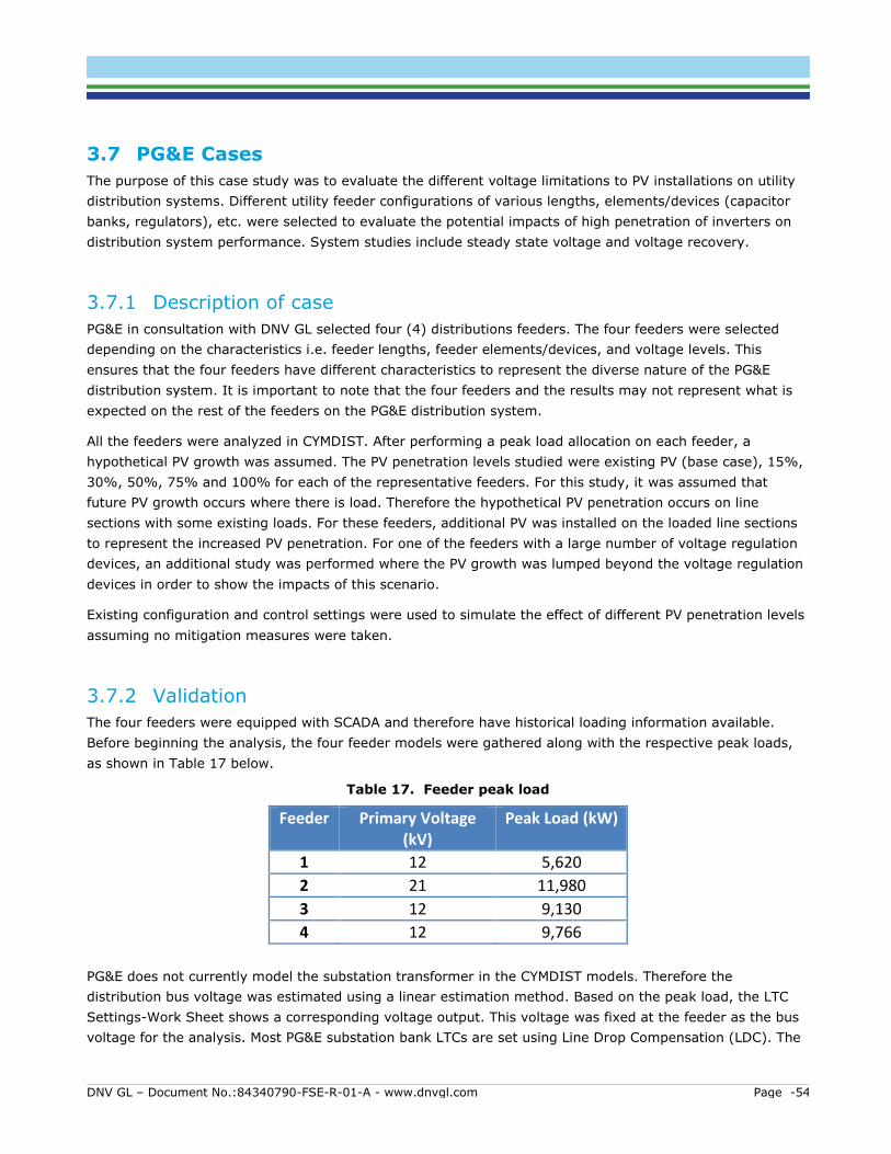
DNV GL – Document No.:84340790-FSE-R-01-A - www.dnvgl.com Page -54
3.7 PG&E Cases
The purpose of this case study was to evaluate the different voltage limitations to PV installations on utility
distribution systems. Different utility feeder configurations of various lengths, elements/devices (capacitor
banks, regulators), etc. were selected to evaluate the potential impacts of high penetration of inverters on
distribution system performance. System studies include steady state voltage and voltage recovery.
3.7.1 Description of case
PG&E in consultation with DNV GL selected four (4) distributions feeders. The four feeders were selected
depending on the characteristics i.e. feeder lengths, feeder elements/devices, and voltage levels. This
ensures that the four feeders have different characteristics to represent the diverse nature of the PG&E
distribution system. It is important to note that the four feeders and the results may not represent what is
expected on the rest of the feeders on the PG&E distribution system.
All the feeders were analyzed in CYMDIST. After performing a peak load allocation on each feeder, a
hypothetical PV growth was assumed. The PV penetration levels studied were existing PV (base case), 15%,
30%, 50%, 75% and 100% for each of the representative feeders. For this study, it was assumed that
future PV growth occurs where there is load. Therefore the hypothetical PV penetration occurs on line
sections with some existing loads. For these feeders, additional PV was installed on the loaded line sections
to represent the increased PV penetration. For one of the feeders with a large number of voltage regulation
devices, an additional study was performed where the PV growth was lumped beyond the voltage regulation
devices in order to show the impacts of this scenario.
Existing configuration and control settings were used to simulate the effect of different PV penetration levels
assuming no mitigation measures were taken.
3.7.2 Validation
The four feeders were equipped with SCADA and therefore have historical loading information available.
Before beginning the analysis, the four feeder models were gathered along with the respective peak loads,
as shown in Table 17 below.
Table 17. Feeder peak load
Feeder Primary Voltage (kV)
Peak Load (kW)
1 12 5,620
2 21 11,980
3 12 9,130
4 12 9,766
PG&E does not currently model the substation transformer in the CYMDIST models. Therefore the
distribution bus voltage was estimated using a linear estimation method. Based on the peak load, the LTC
Settings-Work Sheet shows a corresponding voltage output. This voltage was fixed at the feeder as the bus
voltage for the analysis. Most PG&E substation bank LTCs are set using Line Drop Compensation (LDC). The
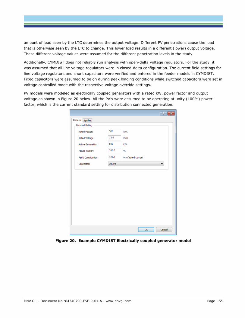
DNV GL – Document No.:84340790-FSE-R-01-A - www.dnvgl.com Page -55
amount of load seen by the LTC determines the output voltage. Different PV penetrations cause the load
that is otherwise seen by the LTC to change. This lower load results in a different (lower) output voltage.
These different voltage values were assumed for the different penetration levels in the study.
Additionally, CYMDIST does not reliably run analysis with open-delta voltage regulators. For the study, it
was assumed that all line voltage regulators were in closed-delta configuration. The current field settings for
line voltage regulators and shunt capacitors were verified and entered in the feeder models in CYMDIST.
Fixed capacitors were assumed to be on during peak loading conditions while switched capacitors were set in
voltage controlled mode with the respective voltage override settings.
PV models were modeled as electrically coupled generators with a rated kW, power factor and output
voltage as shown in Figure 20 below. All the PV’s were assumed to be operating at unity (100%) power
factor, which is the current standard setting for distribution connected generation.
Figure 20. Example CYMDIST Electrically coupled generator model
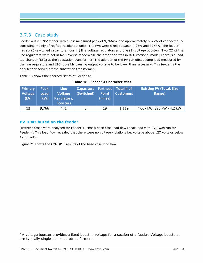
DNV GL – Document No.:84340790-FSE-R-01-A - www.dnvgl.com Page -56
3.7.3 Case study
Feeder 4 is a 12kV feeder with a last measured peak of 9,766kW and approximately 667kW of connected PV
consisting mainly of rooftop residential units. The PVs were sized between 4.2kW and 326kW. The feeder
has six (6) switched capacitors, four (4) line voltage regulators and one (1) voltage booster2. Two (2) of the
line regulators were set in No-Reverse mode while the other one was in Bi-Directional mode. There is a load
tap changer (LTC) at the substation transformer. The addition of the PV can offset some load measured by
the line regulators and LTC, possibly causing output voltage to be lower than necessary. This feeder is the
only feeder served off the substation transformer.
Table 18 shows the characteristics of Feeder 4:
Table 18. Feeder 4 Characteristics
Primary Voltage
(kV)
Peak Load (kW)
Line Voltage
Regulators, Boosters
Capacitors (Switched)
Farthest Point
(miles)
Total # of Customers
Existing PV (Total, Size Range)
12 9,766 4, 1 6 19 1,119 ~667 kW, 326 kW - 4.2 kW
PV Distributed on the feeder
Different cases were analyzed for Feeder 4. First a base case load flow (peak load with PV) was run for
Feeder 4. This load flow revealed that there were no voltage violations i.e. voltage above 127 volts or below
120.5 volts.
Figure 21 shows the CYMDIST results of the base case load flow.
2 A voltage booster provides a fixed boost in voltage for a section of a feeder. Voltage boosters
are typically single-phase autotransformers.
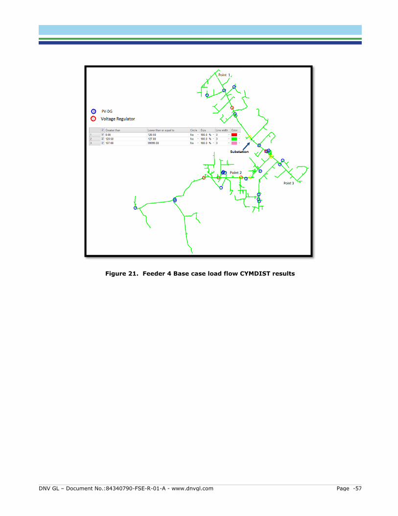
DNV GL – Document No.:84340790-FSE-R-01-A - www.dnvgl.com Page -57
Figure 21. Feeder 4 Base case load flow CYMDIST results
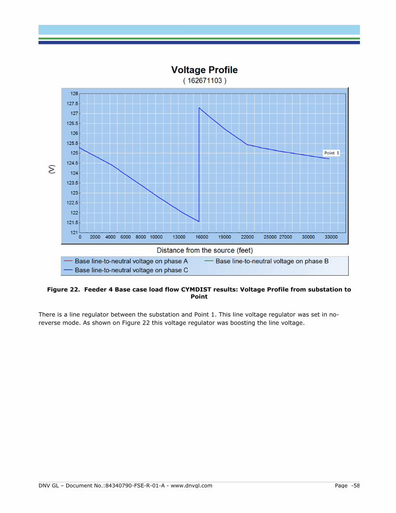
DNV GL – Document No.:84340790-FSE-R-01-A - www.dnvgl.com Page -58
Figure 22. Feeder 4 Base case load flow CYMDIST results: Voltage Profile from substation to Point
There is a line regulator between the substation and Point 1. This line voltage regulator was set in no-
reverse mode. As shown on Figure 22 this voltage regulator was boosting the line voltage.
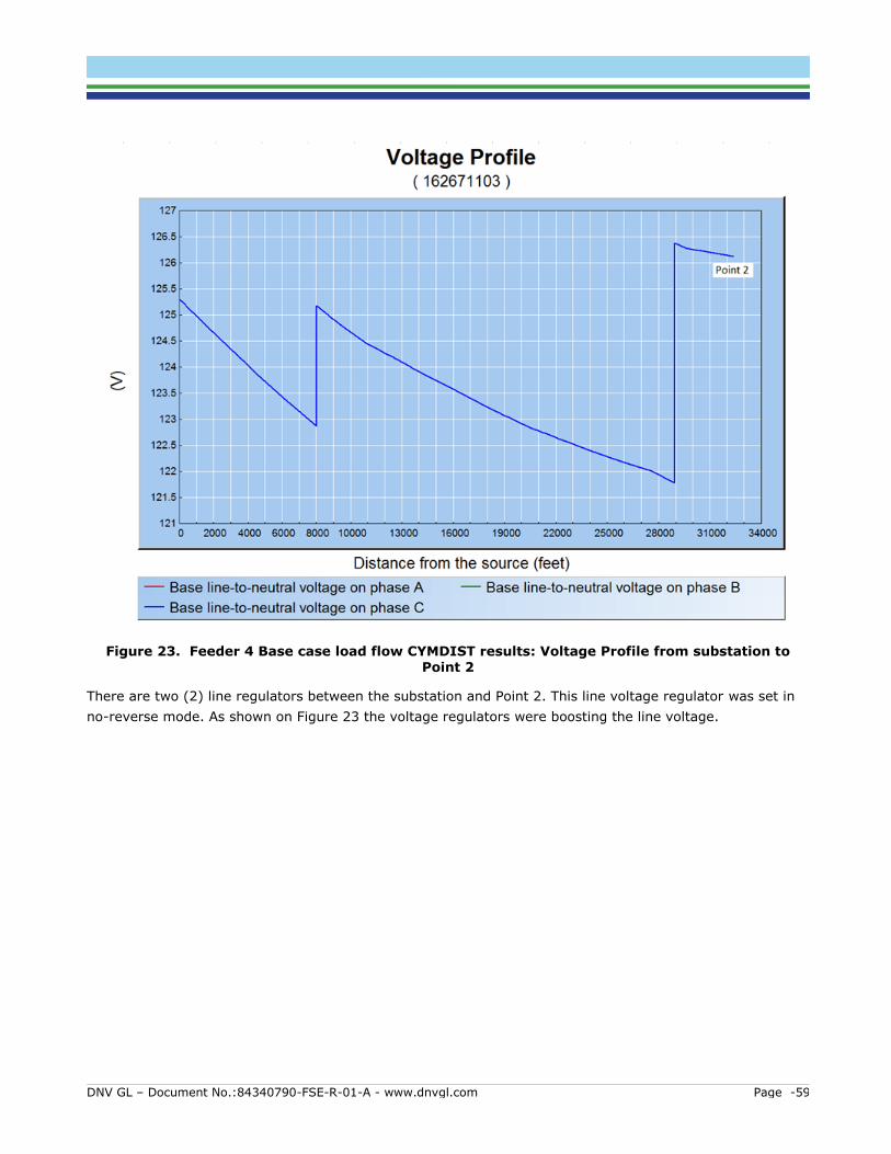
DNV GL – Document No.:84340790-FSE-R-01-A - www.dnvgl.com Page -59
Figure 23. Feeder 4 Base case load flow CYMDIST results: Voltage Profile from substation to Point 2
There are two (2) line regulators between the substation and Point 2. This line voltage regulator was set in
no-reverse mode. As shown on Figure 23 the voltage regulators were boosting the line voltage.
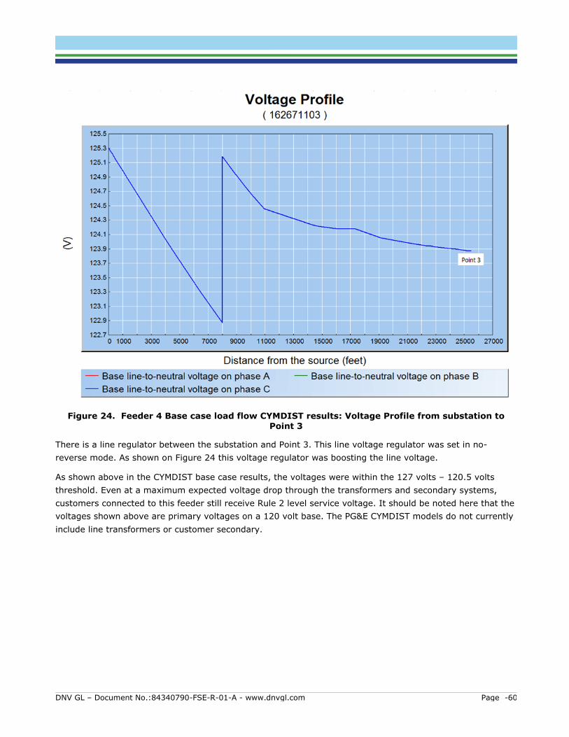
DNV GL – Document No.:84340790-FSE-R-01-A - www.dnvgl.com Page -60
Figure 24. Feeder 4 Base case load flow CYMDIST results: Voltage Profile from substation to Point 3
There is a line regulator between the substation and Point 3. This line voltage regulator was set in no-
reverse mode. As shown on Figure 24 this voltage regulator was boosting the line voltage.
As shown above in the CYMDIST base case results, the voltages were within the 127 volts – 120.5 volts
threshold. Even at a maximum expected voltage drop through the transformers and secondary systems,
customers connected to this feeder still receive Rule 2 level service voltage. It should be noted here that the
voltages shown above are primary voltages on a 120 volt base. The PG&E CYMDIST models do not currently
include line transformers or customer secondary.
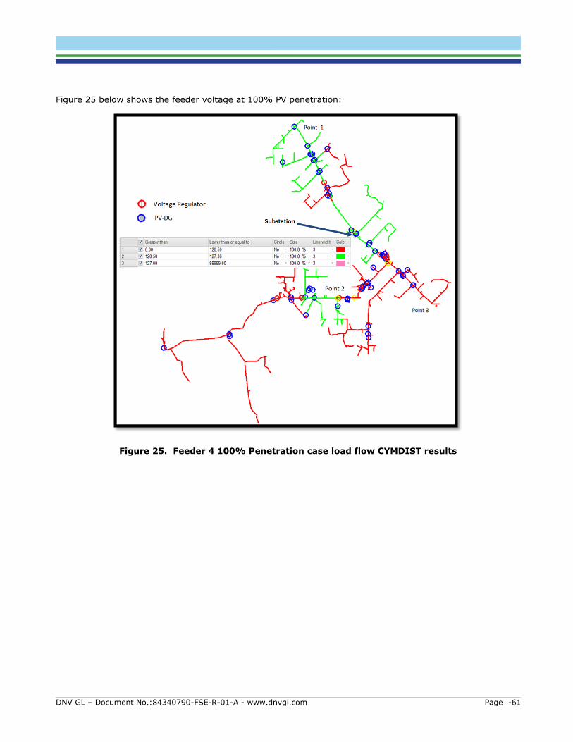
DNV GL – Document No.:84340790-FSE-R-01-A - www.dnvgl.com Page -61
Figure 25 below shows the feeder voltage at 100% PV penetration:
Figure 25. Feeder 4 100% Penetration case load flow CYMDIST results
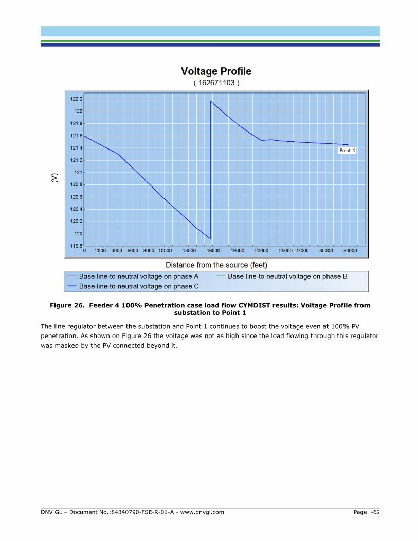
DNV GL – Document No.:84340790-FSE-R-01-A - www.dnvgl.com Page -62
Figure 26. Feeder 4 100% Penetration case load flow CYMDIST results: Voltage Profile from substation to Point 1
The line regulator between the substation and Point 1 continues to boost the voltage even at 100% PV
penetration. As shown on Figure 26 the voltage was not as high since the load flowing through this regulator
was masked by the PV connected beyond it.
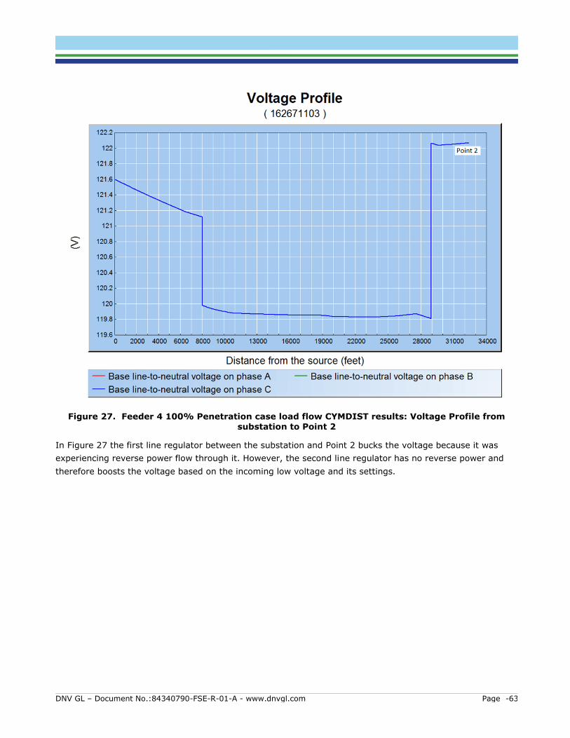
DNV GL – Document No.:84340790-FSE-R-01-A - www.dnvgl.com Page -63
Figure 27. Feeder 4 100% Penetration case load flow CYMDIST results: Voltage Profile from substation to Point 2
In Figure 27 the first line regulator between the substation and Point 2 bucks the voltage because it was
experiencing reverse power flow through it. However, the second line regulator has no reverse power and
therefore boosts the voltage based on the incoming low voltage and its settings.

DNV GL – Document No.:84340790-FSE-R-01-A - www.dnvgl.com Page -64
Figure 28. Feeder 4 100% Penetration case load flow CYMDIST results: Voltage Profile from substation to Point 3
Due to the reverse power flow through the line regulator between the substation and Point 3, the line
regulator bucks the voltage instead of boosting it as was shown in Figure 28 (base case).
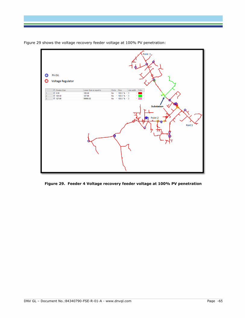
DNV GL – Document No.:84340790-FSE-R-01-A - www.dnvgl.com Page -65
Figure 29 shows the voltage recovery feeder voltage at 100% PV penetration:
Figure 29. Feeder 4 Voltage recovery feeder voltage at 100% PV penetration
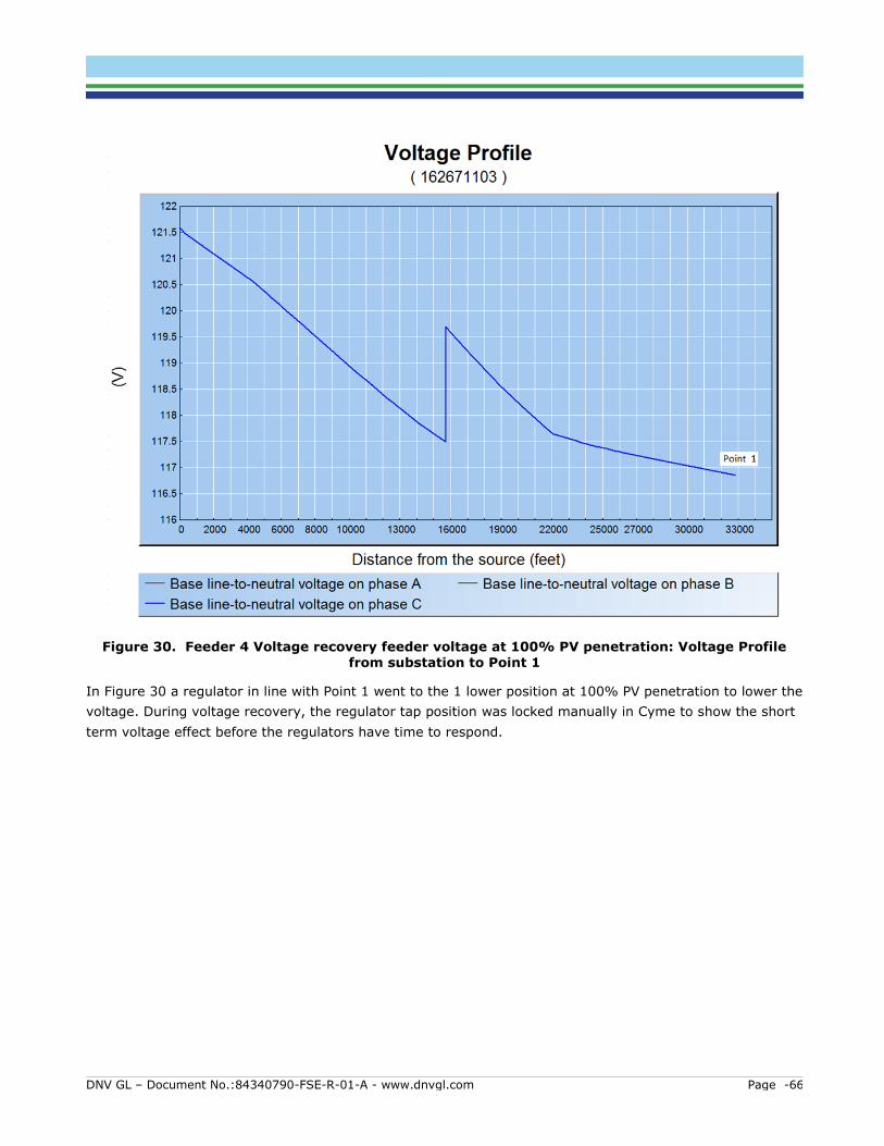
DNV GL – Document No.:84340790-FSE-R-01-A - www.dnvgl.com Page -66
Figure 30. Feeder 4 Voltage recovery feeder voltage at 100% PV penetration: Voltage Profile from substation to Point 1
In Figure 30 a regulator in line with Point 1 went to the 1 lower position at 100% PV penetration to lower the
voltage. During voltage recovery, the regulator tap position was locked manually in Cyme to show the short
term voltage effect before the regulators have time to respond.
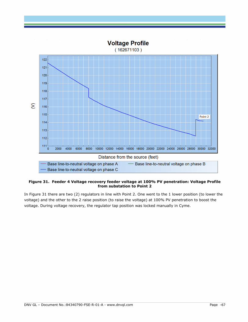
DNV GL – Document No.:84340790-FSE-R-01-A - www.dnvgl.com Page -67
Figure 31. Feeder 4 Voltage recovery feeder voltage at 100% PV penetration: Voltage Profile from substation to Point 2
In Figure 31 there are two (2) regulators in line with Point 2. One went to the 1 lower position (to lower the
voltage) and the other to the 2 raise position (to raise the voltage) at 100% PV penetration to boost the
voltage. During voltage recovery, the regulator tap position was locked manually in Cyme.
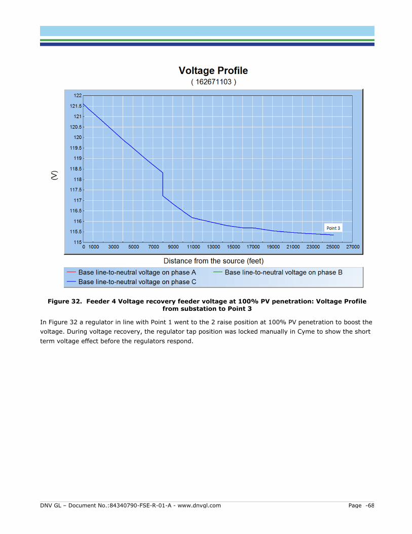
DNV GL – Document No.:84340790-FSE-R-01-A - www.dnvgl.com Page -68
Figure 32. Feeder 4 Voltage recovery feeder voltage at 100% PV penetration: Voltage Profile from substation to Point 3
In Figure 32 a regulator in line with Point 1 went to the 2 raise position at 100% PV penetration to boost the
voltage. During voltage recovery, the regulator tap position was locked manually in Cyme to show the short
term voltage effect before the regulators respond.
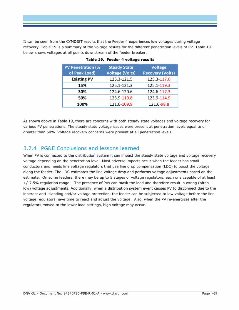
DNV GL – Document No.:84340790-FSE-R-01-A - www.dnvgl.com Page -69
It can be seen from the CYMDIST results that the Feeder 4 experiences low voltages during voltage
recovery. Table 19 is a summary of the voltage results for the different penetration levels of PV. Table 19
below shows voltages at all points downstream of the feeder breaker.
Table 19. Feeder 4 voltage results
PV Penetration (% of Peak Load)
Steady State Voltage (Volts)
Voltage Recovery (Volts)
Existing PV 125.3-121.5 125.3-117.0
15% 125.1-121.3 125.1-119.3
30% 124.6-120.6 124.6-117.3
50% 123.9-119.8 123.9-114.9
100% 121.6-109.9 121.6-98.8
As shown above in Table 19, there are concerns with both steady state voltages and voltage recovery for
various PV penetrations. The steady state voltage issues were present at penetration levels equal to or
greater than 50%. Voltage recovery concerns were present at all penetration levels.
3.7.4 PG&E Conclusions and lessons learned
When PV is connected to the distribution system it can impact the steady state voltage and voltage recovery
voltage depending on the penetration level. Most adverse impacts occur when the feeder has small
conductors and needs line voltage regulators that use line drop compensation (LDC) to boost the voltage
along the feeder. The LDC estimates the line voltage drop and performs voltage adjustments based on the
estimate. On some feeders, there may be up to 5 stages of voltage regulators, each one capable of at least
+/-7.5% regulation range. The presence of PVs can mask the load and therefore result in wrong (often
low) voltage adjustments. Additionally, when a distribution system event causes PV to disconnect due to the
inherent anti-islanding and/or voltage protection, the feeder can be subjected to low voltage before the line
voltage regulators have time to react and adjust the voltage. Also, when the PV re-energizes after the
regulators moved to the lower load settings, high voltage may occur.

DNV GL – Document No.:84340790-FSE-R-01-A - www.dnvgl.com Page -70
4 OVERALL CONCLUSIONS AND RECOMMENDATIONS
As described in the various study sections of this report, utilities of difference sizes and system
configurations were incorporated to test the Proactive Approach and study procedures. Each utility selected
unique renewable penetration scenarios to validate and test the methodology. Through the development,
testing, refinement and application of this methodology, as described in section 3 of this report, several
lessons were learned which have been compiled into the recommendations and conclusions listed in this
section.
The modeling techniques and lessons learned from the work described in this report are applicable to all
utilities contending with challenges (planning, operating & mitigating) of future high penetration issues
related to DG. As part of the review process for Proactive Approach, industry subject matter experts from
utility and organizations like EPRI provided support for a new process that integrates simulation based
modeling capability and data-driven analysis.
Recommendations for enabling the capabilities of the Proactive Approach include:
Organizational alignment and staff to support and maintain baseline model capabilities;
Process coordination with resource procurement;
Establish regular and timely system-wide reviews to update conditions;
Establish timeframe to conduct baseline planning studies and coordinate with industry;
Revised standards with guidance on procedures for modeling and data analysis;
Support and prioritize ongoing grid and resource monitoring for modeling needs;
Enhance modeling tools with device models to capture future “smart” capabilities;
Maintain this capability through appropriate and consistent workforce training.
Some of the most important conclusions are listed below.
Not all feeders have consistent data in the same format. Some have one second data, others
hourly, monthly or no data. However, with the large number of feeders, feeder profiles can be
developed to conduct a high solar penetration study. This data variability demonstrates the need for
a utility to plan ahead for the installation of data recorders to gather consistent, reliable data for
these types of studies.
The location of the distributed solar installations whether at the beginning or end of the feeder
impact the voltage profiles across the feeder
The location and operation of line capacitors and line regulators has an adverse impact on voltages
and line loadings under high solar penetrations. The utility may need to conduct a detailed
coordination study to determine the relocation and operation of these devices.
The setting of the time delays of substation transformer LTC in conjunction with high solar
penetrations can create short periods of high or low voltages on line sections of feeders. If the time
delays between tap movements are short, then there could be excessive LTC operations and varying
DNV GL – Document No.:84340790-FSE-R-01-A - www.dnvgl.com Page -71
feeder voltages. If the time delays are long, there could be low or high line section voltages that
exceed standard limits
The load balance between substation banks may not be equal. This difference can create different
time periods when backfeed occurs through one bank transformer but not the other. The impact of
these differences is important depending on the substation bus configurations and the open bus tie
locations and positions. This can create circulating current, improper LTC operation, switching
problems during emergency and maintenance periods and other issues.
High voltages occurred during solar ramp-ups following an outage incident when the solar restarted
from 0% to 100% generation or during a sudden change in weather patterns that caused partially
generating solar inverters to increase power from 30% to 100%. In all of these cases, the LTC was
unable to respond fast enough to adjust the feeder voltages.
Before starting a distributed solar study, the engineer must make sure that the base case conditions
are well defined, accurate data collected, and the system is operating in the most optimal manner.
When PV is connected to the distribution system it can impact the steady state voltage and voltage
recovery voltage depending on the penetration level. Most adverse impacts occur when the feeder
has small conductors and needs line voltage regulators that use LDC to boost the voltage along the
feeder. The LDC estimates the line voltage drop and performs voltage adjustments based on the
estimate. The presence of PVs can mask the load and therefore result in wrong (often low) voltage
adjustments.
When a distribution system event causes PV to disconnect due to the inherent anti-islanding and/or
voltage protection, the feeder can be subjected to low voltage before the line voltage regulators
have time to react and adjust the voltage. Also, when the PV re-energizes after the regulators
moved to the lower load settings, high voltage may occur.
Maintaining updated baseline simulation models and routinely conducting analysis based on field
data enables utilities to track changes and assess mitigation strategies in a timely fashion across the
overall electric system instead of one project or circuit at a time. Timely and regular review
ensures that baselines used by transmission and distribution planning adequately keep pace with
system and local changes.
5 WHAT IS THE VALUE TO CALIFORNIA UTILITIES
An important question for the California utilities is what does this analysis mean to the utility in determining
the benefits of increasing distributed renewable resources. Some of the important benefits of this study
include:
A repeatable and consistent methodology for evaluating the impacts and benefits of distributed
renewable resources to the utility’s distribution planning process
A methodology that has been proven for any size utility grid with different load forecasts, system
peak demands, service areas, lengths of distribution lines, customer mixes and distribution line
conductor sizes
DNV GL – Document No.:84340790-FSE-R-01-A - www.dnvgl.com Page -72
The study provides a step-by-step approach to distributed renewable penetration studies.
The methodology enables the utility planner to study one individual feeder, a group or regional
group of feeders, entire distribution system and secondary service drops to customer meters
The study provides a list of necessary data requirements and time increments of data to complete
detailed distribution steady state, dynamic and transient studies
The output results can be presented to stakeholders, developers, regulatory agencies to support
distributed renewable penetration recommendations
The methodology can be completed using any detailed distribution planning software such as
Synergi
The methodology has been successfully used by the Hawaii Electric Utilities (HECO, MECO and
HELCO), Sacramento Municipal Utility District, Pacific Gas & Electric, and City of Roseville
The methodology has been applied by other utilities in the States and the Caribbean to conduct
distribution studies
6 WHAT IS THE VALUE TO RESIDENTIAL, COMMERCIAL AND
INDUSTRIAL RATEPAYERS
The majority of the report discusses the benefits to the electric utility and alludes to the benefits to the
residential, commercial and industrial customers. Since the methodology and results of the study produce
results down to the individual secondary meter or a group of secondary meters such as a housing
development, there are benefits to the ratepayers that include:
A proven methodology acceptable to both the utility and the regulatory agency that shows positive
and negative impacts to high penetrations of renewables in a particular service area or to a region.
The ratepayers can visually see the impacts to voltage, frequency, and dynamic impacts from the
installation of a large or group of large rooftop solar systems in one local area.
The ratepayers can understand that there is an actual limit to the size of a solar system that can be
installed without causing reliability issues to their neighbors, utility and themselves.
The ratepayers have access to information from the utility to assist in their discussions with the solar
developers and installers to prevent too large a system to be installed that reduces the value to the
ratepayers due to lack of full benefits of over-building.
If local upgrades to the distribution system are required, the utility staff and ratepayers can find
potential solutions and the respective costs, including customer owned storage, that the parties can
mutually agree to make to increase solar benefits without reducing reliability to the ratepayers and
their neighbors.
Information to ratepayers can be provided through outreach programs, regional workshops, direct
meetings with utility staff, commission or agency workshops or other programs.
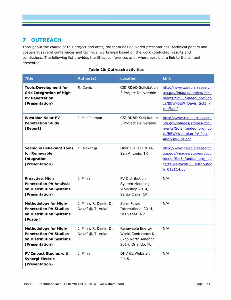
DNV GL – Document No.:84340790-FSE-R-01-A - www.dnvgl.com Page -73
7 OUTREACH
Throughout the course of this project and after, the team has delivered presentations, technical papers and
posters at several conferences and technical workshops based on the work conducted, results and
conclusions. The following list provides the titles, conferences and, where possible, a link to the content
presented.
Table 20: Outreach activities
Title Author(s) Location Link
Tools Development for
Grid Integration of High
PV Penetration
(Presentation)
R. Davis CSI RD&D Solicitation
3 Project Deliverable
http://www.calsolarresearch
.ca.gov/images/stories/docu
ments/Sol3_funded_proj_do
cs/BEW/BEW_Davis_Sol3_ki
ckoff.pdf
Westplan Solar PV
Penetration Study
(Report)
J. MacPherson CSI RD&D Solicitation
3 Project Deliverable
http://www.calsolarresearch
.ca.gov/images/stories/docu
ments/Sol3_funded_proj_do
cs/BEW/Westplan-PV-Pen-
Analysis-Rpt.pdf
Seeing is Believing! Tools
for Renewable
Integration
(Presentation)
D. Nakafuji DistribuTECH 2014,
San Antonio, TX
http://www.calsolarresearch
.ca.gov/images/stories/docu
ments/Sol3_funded_proj_do
cs/BEW/Nakafuji_Distributec
h_012114.pdf
Proactive, High
Penetration PV Analysis
on Distribution Systems
(Presentation)
J. Flinn PV Distribution
System Modeling
Workshop 2014,
Santa Clara, CA
N/A
Methodology for High-
Penetration PV Studies
on Distribution Systems
(Poster)
J. Flinn, R. Davis, D.
Nakafuji, T. Aukai
Solar Power
International 2014,
Las Vegas, NV
N/A
Methodology for High-
Penetration PV Studies
on Distribution Systems
(Presentation)
J. Flinn, R. Davis, D.
Nakafuji, T. Aukai
Renewable Energy
World Conference &
Expo North America
2014, Orlando, FL
N/A
PV Impact Studies with
Synergi Electric
(Presentation)
J. Flinn DNV GL Webinar,
2015
N/A
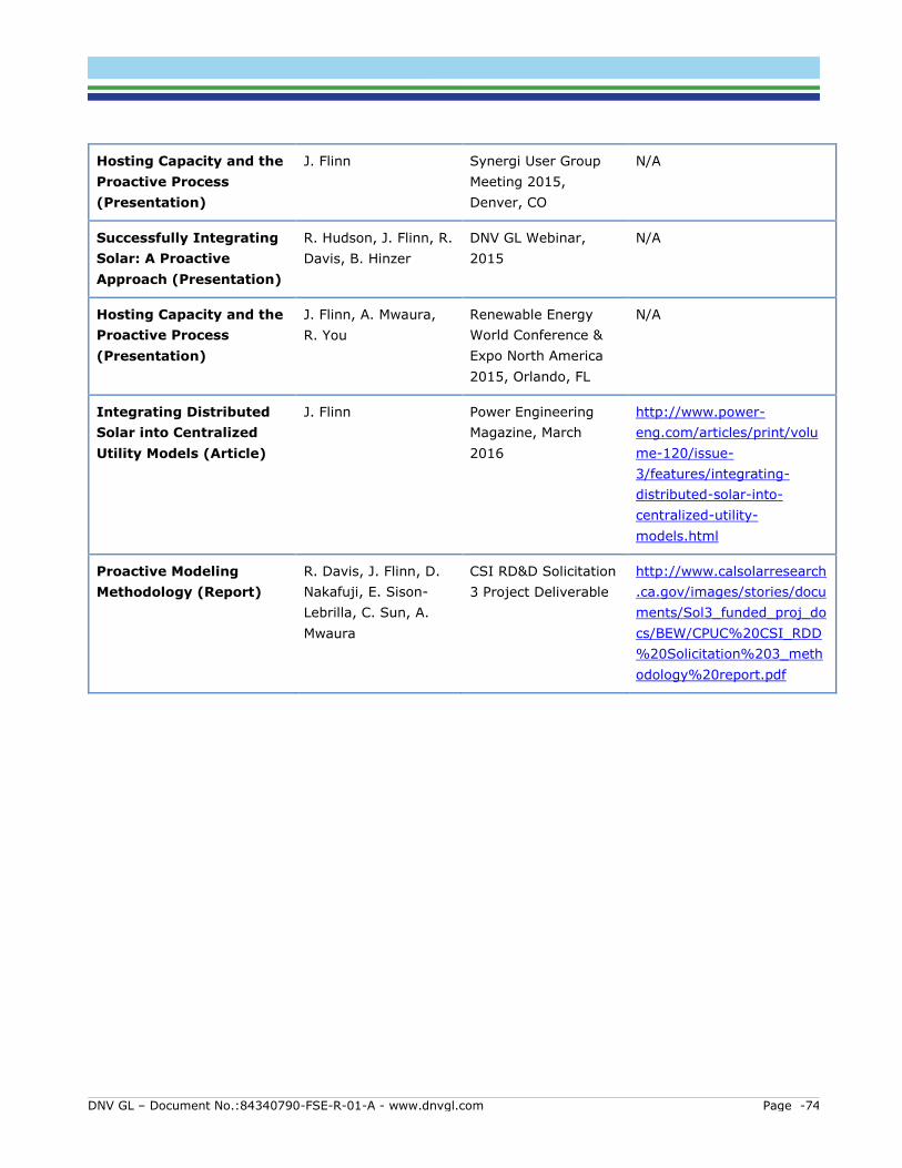
DNV GL – Document No.:84340790-FSE-R-01-A - www.dnvgl.com Page -74
Hosting Capacity and the
Proactive Process
(Presentation)
J. Flinn Synergi User Group
Meeting 2015,
Denver, CO
N/A
Successfully Integrating
Solar: A Proactive
Approach (Presentation)
R. Hudson, J. Flinn, R.
Davis, B. Hinzer
DNV GL Webinar,
2015
N/A
Hosting Capacity and the
Proactive Process
(Presentation)
J. Flinn, A. Mwaura,
R. You
Renewable Energy
World Conference &
Expo North America
2015, Orlando, FL
N/A
Integrating Distributed
Solar into Centralized
Utility Models (Article)
J. Flinn Power Engineering
Magazine, March
2016
http://www.power-
eng.com/articles/print/volu
me-120/issue-
3/features/integrating-
distributed-solar-into-
centralized-utility-
models.html
Proactive Modeling
Methodology (Report)
R. Davis, J. Flinn, D.
Nakafuji, E. Sison-
Lebrilla, C. Sun, A.
Mwaura
CSI RD&D Solicitation
3 Project Deliverable
http://www.calsolarresearch
.ca.gov/images/stories/docu
ments/Sol3_funded_proj_do
cs/BEW/CPUC%20CSI_RDD
%20Solicitation%203_meth
odology%20report.pdf
ABOUT DNV GL Driven by our purpose of safeguarding life, property and the environment, DNV GL enables organizations to advance the safety and sustainability of their business. We provide classification and technical assurance
along with software and independent expert advisory services to the maritime, oil and gas, and energy industries. We also provide certification services to customers across a wide range of industries. Operating in more than 100 countries, our 16,000 professionals are dedicated to helping our customers make the world safer, smarter, and greener.