1

High Energy Polarimetry of Positron Beams

Dave GaskellJefferson Lab

International Workshop on Physics with Positrons at Jefferson Lab

September 12-15, 2017

1. Electron polarimetry at High Energies and at JLab• Techniques• Overview of devices

2. Application of electron techniques and devices for positron beams

2

JLab Polarimetry Techniques• Three different processes used to measure electron beam

polarization at JLab– Møller scattering: , atomic electrons in Fe (or

Fe-alloy) polarized using external magnetic field– Compton scattering: , laser photons scatter

from electron beam– Mott scattering: , spin-orbit coupling of electron

spin with (large Z) target nucleus• Each has advantages and disadvantages in JLab environment

eeee +®+!!

gg +®+ ee !!

eZe ®+!

Method Advantage Disadvantage

Compton Non-destructive, precise Can be time consuming, systematics energy dependent

Møller Rapid, precise measurements Destructive, low current only

Mott Rapid, precise measurements Does not measure polarization at the experiment

3

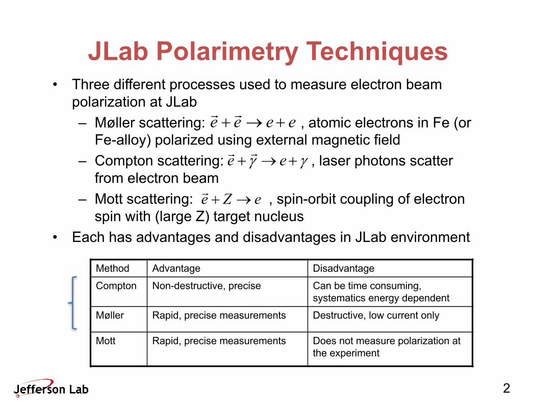
Geography of JLab Polarimeters

A B C

D

Injector

Injector5 MeV Mott Polarimeter

Hall ACompton Polarimeter• IR à Green laserMøller Polarimeter• In plane, low field

target à out of plane saturated iron foil

Hall CCompton Polarimeter• Installed 2010 (Q-Weak)Møller Polarimeter• Out of plane saturated

iron foil

Hall BMøller Polarimeter• In plane, low field

target

4

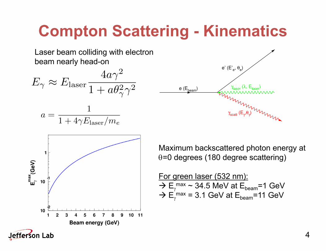
Compton Scattering - Kinematics

e (Ebeam)

γscatt (Eγ,θγ)

γlaser (λ, Elaser)

e’ (E’e, θe)

E� ⇡ Elaser4a�2

1 + a✓2��2

a =1

1 + 4�Elaser/me

Maximum backscattered photon energy atq=0 degrees (180 degree scattering)

For green laser (532 nm):à Eg

max ~ 34.5 MeV at Ebeam=1 GeVà Eg

max = 3.1 GeV at Ebeam=11 GeV

Laser beam colliding with electron beam nearly head-on

5

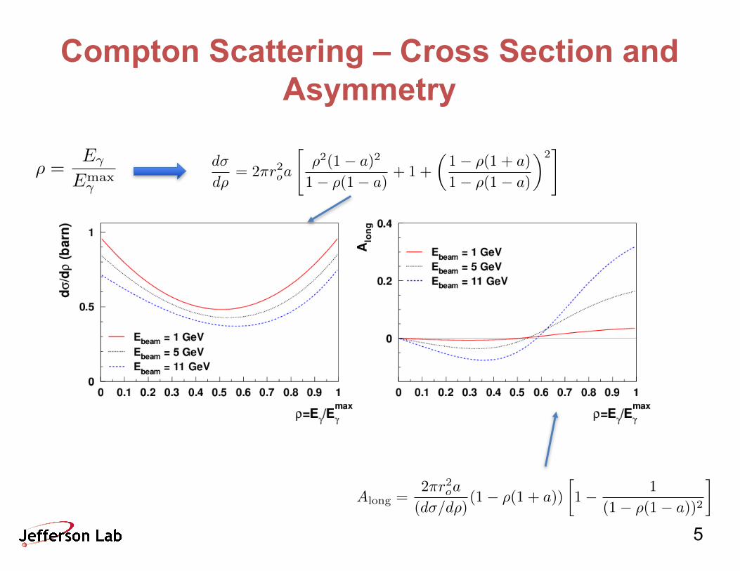
Compton Scattering – Cross Section and Asymmetry

d�

d⇢= 2⇡r2

o

a

"⇢2(1� a)2

1� ⇢(1� a)+ 1 +

✓1� ⇢(1 + a)

1� ⇢(1� a)

◆2#

⇢ =E�

Emax

�

Along

=2⇡r2

o

a

(d�/d⇢)(1� ⇢(1 + a))

1� 1

(1� ⇢(1� a))2

�

6

Compton Polarimetry at JLab• Compton polarimetry routinely used at colliders/storage rings before

use at JLab

• Several challenges for use at JLab – Low beam currents (~100 µA) compared to colliders

• Measurements can take on the order of hours• Makes systematic studies difficult

– At lower energies, relatively small asymmetries• Smaller asymmetries lead to harder-to-control systematics

• Strong dependence of asymmetry on Eg leads to non-trivial determination of analyzing power– Understanding the detector response crucial

7

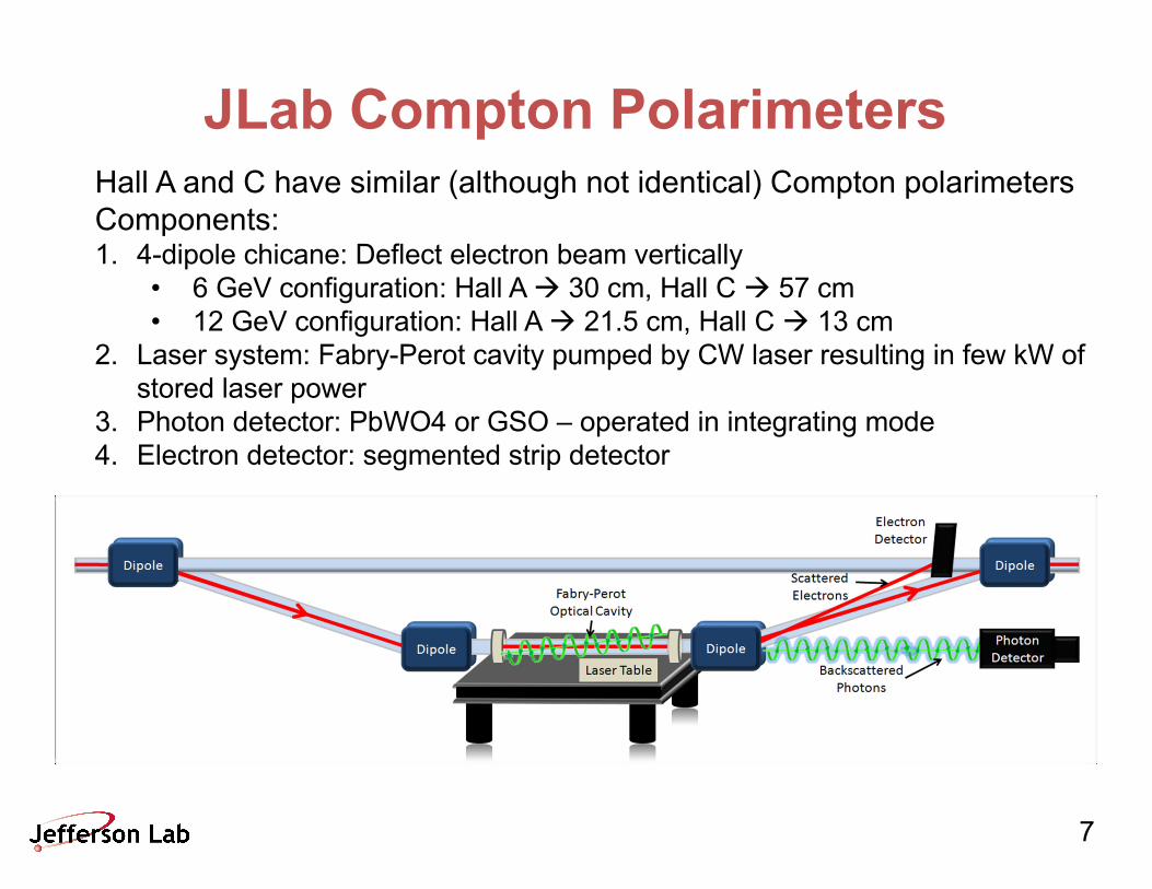
JLab Compton PolarimetersHall A and C have similar (although not identical) Compton polarimetersComponents:1. 4-dipole chicane: Deflect electron beam vertically

• 6 GeV configuration: Hall A à 30 cm, Hall C à 57 cm• 12 GeV configuration: Hall A à 21.5 cm, Hall C à 13 cm

2. Laser system: Fabry-Perot cavity pumped by CW laser resulting in few kW of stored laser power

3. Photon detector: PbWO4 or GSO – operated in integrating mode 4. Electron detector: segmented strip detector

8

Compton Polarimetry for Positrons at JLab

• Compton polarimetry can be almost trivially applied to positron beams– Cross sections, analyzing power identical– Polarimeter layout (dipole chicane, detectors, etc.)

needs no modifications à just need to flip polarity of dipoles in chicane

• The only significant challenge is the relatively low rates• Deploying Compton polarimeter in Hall B would be

difficult (real estate and cost) à might be limited to using existing Comptons in Halls A and C

9

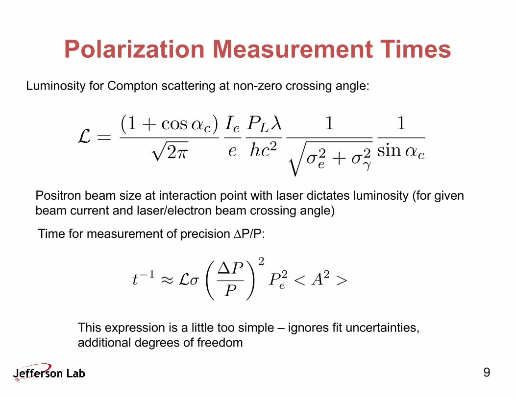
Polarization Measurement TimesLuminosity for Compton scattering at non-zero crossing angle:

L =

(1 + cos↵c)p2⇡

Iee

PL�

hc21q

�2e + �2

�

1

sin↵c

Positron beam size at interaction point with laser dictates luminosity (for given beam current and laser/electron beam crossing angle)

Time for measurement of precision DP/P:

t�1 ⇡ L�✓�P

P

◆2

P 2e < A2 >

This expression is a little too simple – ignores fit uncertainties, additional degrees of freedom

10

Polarization Measurement TimesUse Q-Weak experience to deduce realistic measurement times for “positron Compton”

Q-Weak:Ebeam = 1.16 GeV, P~ 89%, PLaser=1.7 kW,Ibeam = 180 uA:à Rate ~ 150 kHz, à dP/P = 0.47% in 1 hour run (laser off half the time for background measurements)

Assume comparable beam size for 11 GeV positrons, P~ 60%, 100 nA, higher power laser (5 kW)

à Rate ~ 185 Hzà dP/P ~ 3% for 1 hour run

dP/P = 1% would require ~ 9 hoursà This is “best case” scenario. Lower polarization, energy, beam current all lead to longer measurement times

11

Compton Polarimetry for Positrons• Compton polarimeters in Halls A and C can in principle

be used for positrons with no modifications à change polarity of dipole string

• Measurements times are significant – Compton polarimeters envisioned for use with beam currents > 1 µA– Shorter measurement times would require higher

power laser system– 10 kW FP cavities have been achieved at JLab – not

routine– Alternate laser system with mode-locked laser locked

to FP cavity could provide higher luminosity

12

RF pulsed FP Cavity

Crossing angle (deg.)

Lu

min

os

ity

(c

m-2

s-1

)

0

2000

4000

6000

x 10 27

0.5 1 1.5 2 2.5 3

RF pulsed laser

CW laser

RF pulsed cavities have been built – this is a technology under development for ILC among other applications

JLab beam à 499 MHz, Dt~0.5 ps

( )1

222

2,

2, )2/(sin

12

-

÷÷ø

öççè

æ+++» lasereeclaserc

CW

pulsed

fc

LL

ssa

ssp tt

Luminosity from pulsed laser drops more slowly with crossing angle than CW laserà FP cavity pumped by mode-

locked laser at beam frequency could yield significantly higher luminosity

à More complicated system –R&D required

Hall A/C lasers

13

Compton Polarimetry at JLEIC

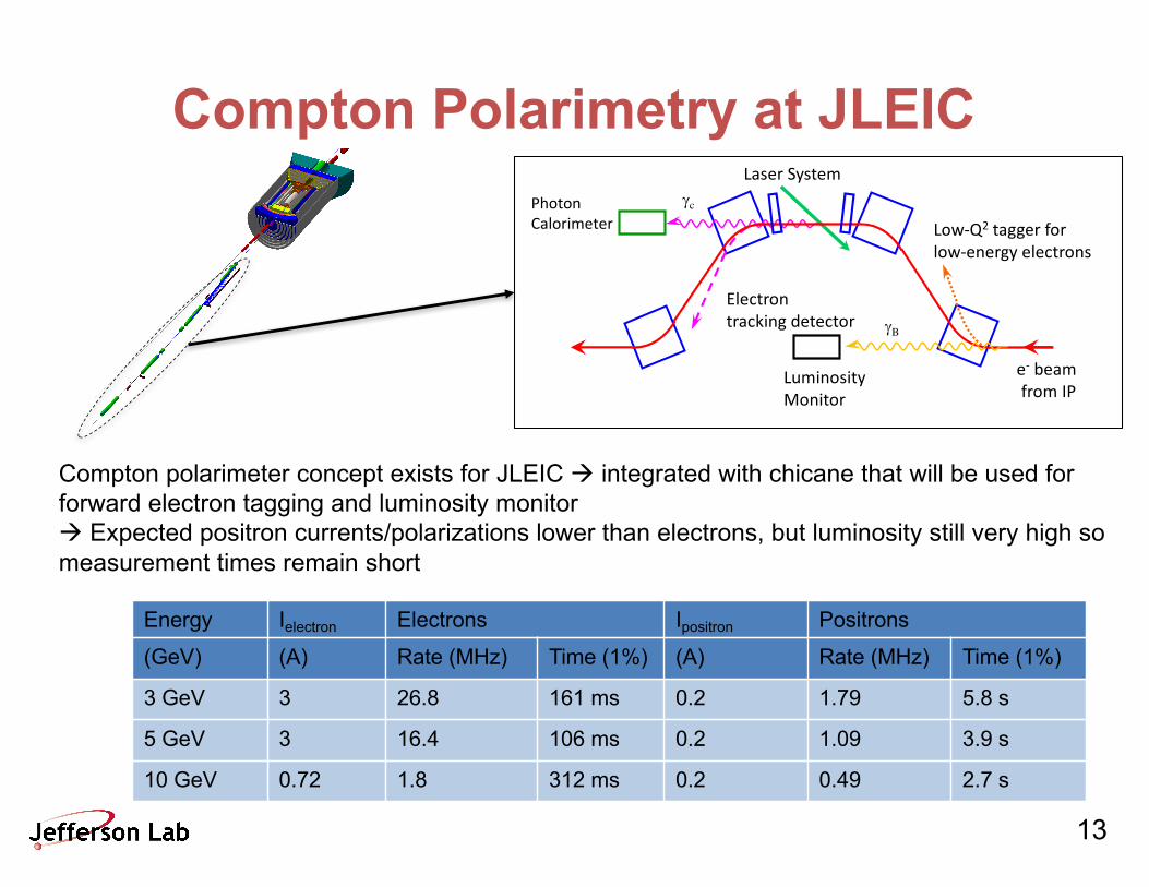
Compton polarimeter concept exists for JLEIC à integrated with chicane that will be used for forward electron tagging and luminosity monitorà Expected positron currents/polarizations lower than electrons, but luminosity still very high so measurement times remain short

gc

LaserSystem

e- beamfromIP

Low-Q2 taggerforlow-energyelectrons

Electrontrackingdetector

PhotonCalorimeter

gB

LuminosityMonitor

Energy Ielectron Electrons Ipositron Positrons

(GeV) (A) Rate (MHz) Time (1%) (A) Rate (MHz) Time (1%)

3 GeV 3 26.8 161 ms 0.2 1.79 5.8 s

5 GeV 3 16.4 106 ms 0.2 1.09 3.9 s

10 GeV 0.72 1.8 312 ms 0.2 0.49 2.7 s

14

Møller PolarimetryElectron beam scatters from (polarized) atomic electrons in atom (typically iron or similar)

Longitudinally polarized electrons/target:

à At q*=90 deg. à -7/9Ak =

�(7 + cos

2 ✓⇤) sin2 ✓⇤

(3 + cos

2 ✓⇤)2

d�

d⌦⇤ =

↵2

s

(3 + cos

2 ✓⇤)2

sin

4 ✓⇤⇥1 + PePtAk(✓

⇤)

⇤

à At q*=90 deg. à -1/9A? =

� sin

4 ✓⇤

(3 + cos

2 ✓⇤)2

Maximum asymmetry independent of beam energy

Transversely polarized electrons/target

15

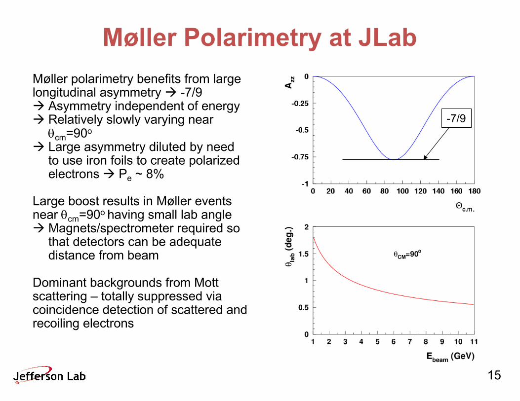
Møller Polarimetry at JLab

-7/9

Møller polarimetry benefits from large longitudinal asymmetry à -7/9à Asymmetry independent of energyà Relatively slowly varying near

qcm=90o

à Large asymmetry diluted by need to use iron foils to create polarized electrons à Pe ~ 8%

Large boost results in Møller events near qcm=90o having small lab angleà Magnets/spectrometer required so

that detectors can be adequate distance from beam

Dominant backgrounds from Mott scattering – totally suppressed via coincidence detection of scattered and recoiling electrons

16

Hall A Møller Polarimeter• Two target systems available

– Supermendeur foil, polarized in-plane, low applied field

– Pure iron foil, polarized out of plan, 3-4 T applies field

• Large acceptance of detectors mitigates potentially large systematic unc. from Levchuk effect (atomic Fermi motion of bound electrons)

• Large acceptance also leads to large rates - dead time corrections cannot be ignored, but are tractable

17

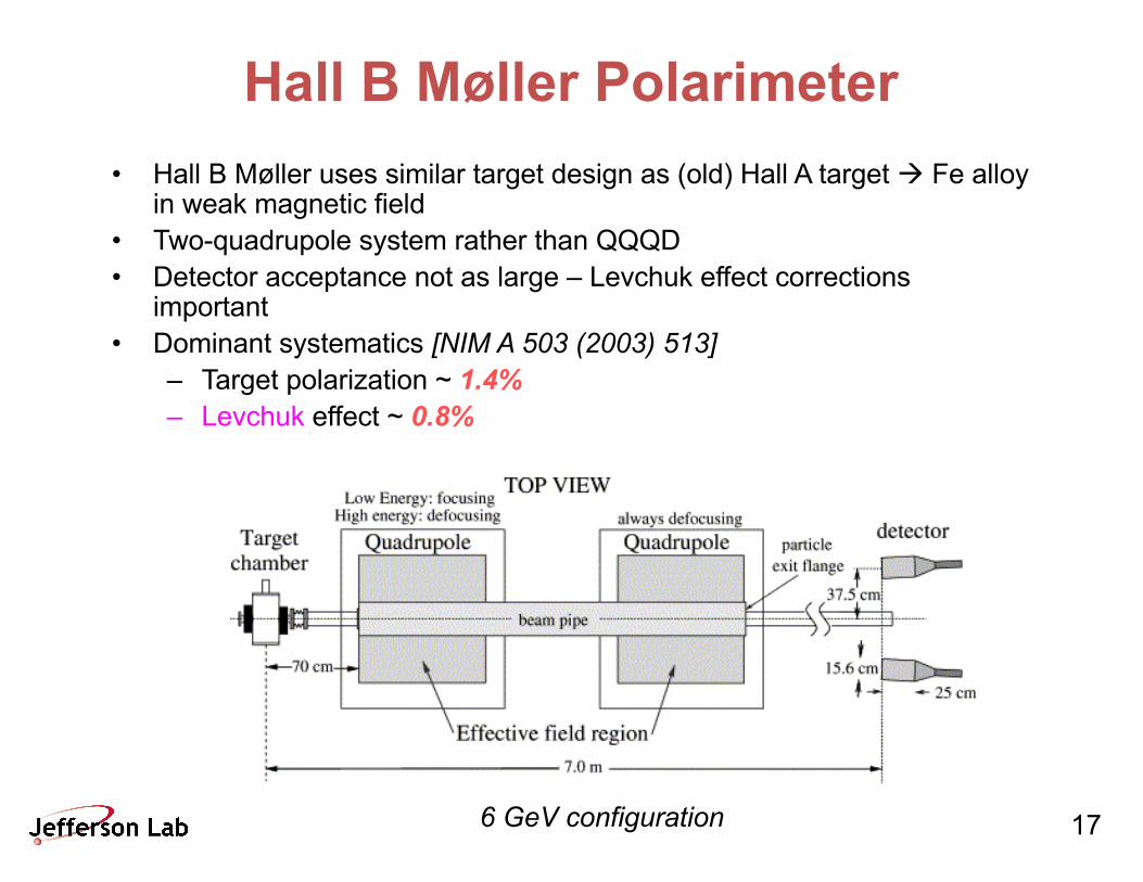
Hall B Møller Polarimeter• Hall B Møller uses similar target design as (old) Hall A target à Fe alloy

in weak magnetic field• Two-quadrupole system rather than QQQD• Detector acceptance not as large – Levchuk effect corrections

important• Dominant systematics [NIM A 503 (2003) 513]

– Target polarization ~ 1.4%– Levchuk effect ~ 0.8%

6 GeV configuration

18

Hall C Møller Polarimeter

!"#$%&%

'(%

')%*+,,-&./+01%

23/3*/+01%

43.&%

/.053/%

1+,36+-2%

("#78%&% 8"(9%&%

(":::%&%

(%&%

'(%

')%*+,,-&./+01%

23/3*/+01%

43.&%

/.053/%

1+,36+-2%

)"()$%&% 8";9$%&%

':%

• 2 quadrupole optics maintains constant tune at detector plane• “Moderate” acceptance mitigates Levchuk effect à still a non-

trivial source of uncertainty• Target = pure Fe foil, brute-force polarized out of plane with 3-4 T

superconducting magnet• Target polarization uncertainty = 0.25% [NIM A 462 (2001) 382]

19

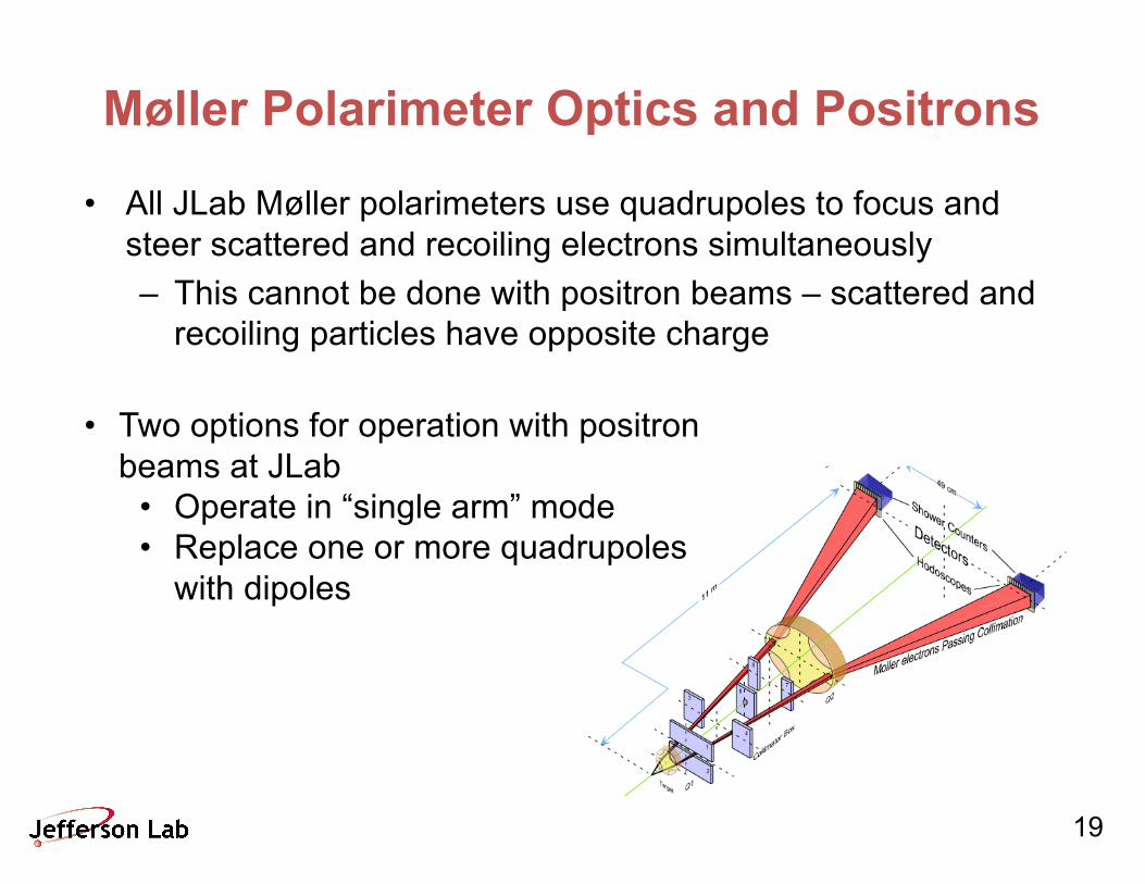
Møller Polarimeter Optics and Positrons

• All JLab Møller polarimeters use quadrupoles to focus and steer scattered and recoiling electrons simultaneously– This cannot be done with positron beams – scattered and

recoiling particles have opposite charge

• Two options for operation with positron beams at JLab

• Operate in “single arm” mode• Replace one or more quadrupoles

with dipoles

20

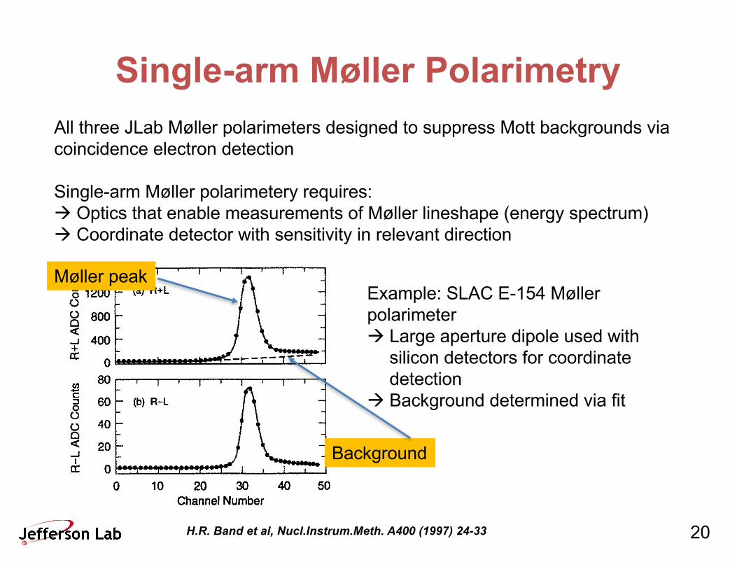
Single-arm Møller PolarimetryAll three JLab Møller polarimeters designed to suppress Mott backgrounds via coincidence electron detection

Single-arm Møller polarimetery requires:à Optics that enable measurements of Møller lineshape (energy spectrum)à Coordinate detector with sensitivity in relevant direction

30 H.R. Band et al. iNuc1. instr. and _Meth. in Phys. Res. A 400 jf997) 24-33

is then proportional to the number of incident Msller electrons.

The silicon channels were connected to 96 charge sensitive preamplifiers [9]. The preamplifiers inte- grated the total charge deposited in each silicon strip over the 250ns beam spill. The preamplifier output was brought to the ESA counting house into SLAC- designed ADC’s. The ADC’s resided in E-154 beam CAMAC crates but were only read out during Moller runs. Linearity calibrations were made before and af- ter the E - 154 data run. Nonlinearities were less than 0.5% and typically less than 0.1% with the exception of one channel in the top detector which is not used in the present analysis.

4. M&er data

The polarized electron beam was produced by photo-emission from a strained GaAs photo-cathode illuminated with circularly polarized light from a flashlamp-pum~d Ti-sapphire laser [lo]. The light helicity was reversed randomly pulse by pulse. The beam helicity for each pulse was tagged by a right(R) or left(L) bit and this information was transmitted to the pola~meter. The beam was accelerated to 48.8GeVjc and delivered to the experiment through SLAC beam-line A. The beam lost 400 MeV of en- ergy due to synchrotron radiation before entering the end station. The electron spin rotates through 7.5 rev- olutions in the A-line thus reversing the beam helicity in the end station relative to the source.

Moller data were taken during special dedicated E-154 runs. Moller data taking required different beam optics from normal E -154 data taking. A quadrupole, between the Moller target and mask, had to be turned off. Upstream quads were then adjusted to maintain reasonable beam sizes. The Moller target was then positioned in the beam and the Moller mag- net was turned on. Moller data runs were typically 10 min and yielded a statistical error of 0.01. Runs were usually taken in pairs with opposite polarity tar- get fields. As the beam quality improved, systematic studies of the pol~zation dependence on the A-line beam energy and the source laser parameters were made, After the longitudinal beam polarization was optimized, the beam polarization was stable.

5. Data analysis

The Mraller analysis proceeded through two steps. The first-pass analysis calculated average pulse heights and errors for each channel from the pulse by pulse data. Separate averages were made for pulses tagged by R and L polarization bits. Corre- lations between channels in the pulse by pulse data were calculated and recorded in a covariance ma- trix. A very loose beam current requirement was made before including the pulse in the overall av- erages. A summary file containing the ADC aver- ages, errors, and correlations, as well as useful beam and polarimeter parameters was written for each run.

A second-pass analysis read the summary file and formed sum (R+L) and difference (R-L) averages and errors for each channel. Typical (R+L) and (R-L) line-shapes for the top detector are shown in Fig. 6.

The background under the unpolarized (R+L) Moller scatters was estimated by fitting the (R+L) lineshape to an arbitrary quadratic background plus the lineshape expected from unpolarized Moller scattering. The technique for estimating the unpo- larized lineshape used the observed R-L line-shape and the angular smearing functions shown in Fig. 1 to generate a predicted R+L line-shape for Moller

u, 1600 E a 1200 0 g 800

4 400 8

0

10 20 30 40 50 Channel Number

Fig. 6. The measured unpolarized (R+L) lineshape (a) and the polarized (R-L) lineshape (b) in the top detector are shown for a typical run. The dashed line is the fitted unpolarized background. The solid line is the fitted unpolarized Mraller line-shape plus background.

H.R. Band et al, Nucl.Instrum.Meth. A400 (1997) 24-33

Example: SLAC E-154 Møllerpolarimeterà Large aperture dipole used with

silicon detectors for coordinate detection

à Background determined via fit

Møller peak

Background

21

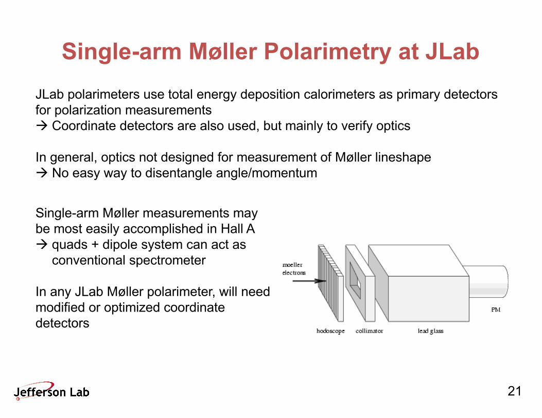
Single-arm Møller Polarimetry at JLabJLab polarimeters use total energy deposition calorimeters as primary detectors for polarization measurements à Coordinate detectors are also used, but mainly to verify optics

In general, optics not designed for measurement of Møller lineshapeà No easy way to disentangle angle/momentum

Single-arm Møller measurements may be most easily accomplished in Hall Aà quads + dipole system can act as

conventional spectrometer

In any JLab Møller polarimeter, will need modified or optimized coordinate detectors

22

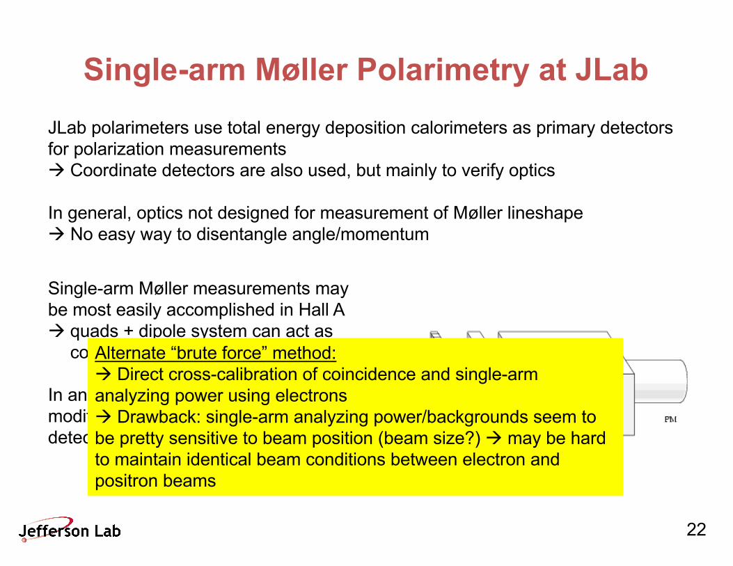
Single-arm Møller Polarimetry at JLabJLab polarimeters use total energy deposition calorimeters as primary detectors for polarization measurements à Coordinate detectors are also used, but mainly to verify optics

In general, optics not designed for measurement of Møller lineshapeà No easy way to disentangle angle/momentum

Single-arm Møller measurements may be most easily accomplished in Hall Aà quads + dipole system can act as

conventional spectrometer

In any JLab Møller polarimeter, will need modified or optimized coordinate detectors

Alternate “brute force” method: à Direct cross-calibration of coincidence and single-arm analyzing power using electronsà Drawback: single-arm analyzing power/backgrounds seem to be pretty sensitive to beam position (beam size?) à may be hard to maintain identical beam conditions between electron and positron beams

23

Møller Polarimetry with e+/e-coincidences

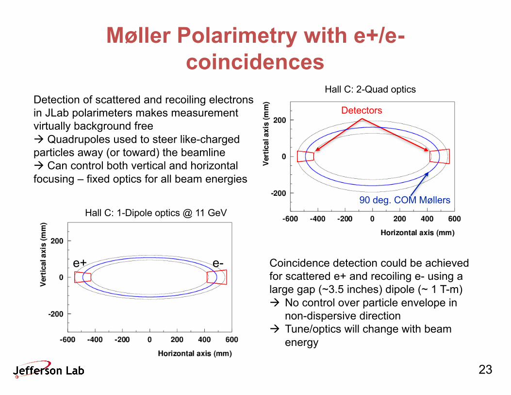
Detection of scattered and recoiling electrons in JLab polarimeters makes measurement virtually background freeà Quadrupoles used to steer like-charged particles away (or toward) the beamlineà Can control both vertical and horizontal focusing – fixed optics for all beam energies

Coincidence detection could be achieved for scattered e+ and recoiling e- using a large gap (~3.5 inches) dipole (~ 1 T-m)à No control over particle envelope in

non-dispersive directionà Tune/optics will change with beam

energy

Detectors

90 deg. COM Møllers

Hall C: 2-Quad optics

Hall C: 1-Dipole optics @ 11 GeV

e+ e-

24

Summary• Compton polarimetry can be used in Halls A and C with the

existing devices virtually unmodified– Measurement times will be long with existing laser system– New laser system (FP cavity pumped by mode-locked

laser) could significantly improve luminosity à R&D would be required

• Møller polarimetry is possible, but some modifications would be required– Operation in single arm (scattered particle only) mode

would require investigation into optimized background suppression à new optics and/or detector system

– Operation in coincidence mode (scattered e+ and recoil e-) would require new magnet à replace one or more quads with dipole