Heat and Power Applications of

Advanced Biomass Gasifiers in New

Zealand’s Wood Industry

A Chemical Equilibrium Model and Economic Feasibility Assessment

A thesis submitted in fulfilment of the requirements for the Degree

of Master of Engineering in Chemical and Process Engineering

University of Canterbury

2006

John Rutherford

i

Abstract

The Biomass Integrated Gasification Application Systems (BIGAS) consortium is a research group whose focus is on developing modern biomass gasification technology for New Zealand’s wood industry. This thesis is undertaken under objective four of the BIGAS consortium, whose goal is to develop modelling tools for aiding in the design of pilot-scale gasification plant and for assessing the economic feasibility of gasification energy plant. This thesis presents a chemical equilibrium-based gasification model and an economic feasibility assessment of gasification energy plant. Chemical equilibrium is proven to accurately predict product gas composition for large scale, greater than one megawatt thermal, updraft gasification. However, chemical equilibrium does not perform as well for small scale, 100 to 150 kilowatt thermal, Fast Internally Circulating Fluidised Bed (FICFB) gasification. Chemical equilibrium provides a number of insights on how altering gasification parameters will affect the composition of the product gas and will provide a useful tool in the design of pilot-scale plant. The economic model gives a basis for judging the optimal process and the overall appeal of integrating biomass gasification-based heat and power plants into New Zealand’s MDF industry. The model is what Gerrard (2000) defines as a ‘study estimate’ model which has a probable range of accuracy of ±20% to ±30%. The modelling results show that gasification-gas engine plants are economically appealing when sized to meet the internal electricity demands of an MDF plant. However, biomass gasification combined cycle plants (BIGCC) and gasification-gas turbine plants are proven to be uneconomic in the New Zealand context.

ii

Acknowledgements

There are a number of people whose efforts and advice helped considerably in the completion of this work. To all these people, I thank you. The following people deserve a special mention:

• Shusheng Pang, without whom the BIGAS consortium would not exist. I thank you for the opportunity of studying as part of the research group.

• Chris Williamson, whose supervision and guidance was invaluable during

the project. • Rick Dobbs and Jock Brown, whose humour, efforts and persistence

enabled the project to reach its current state. The gasifier project owes so much to you two.

• My colleagues (in particular John Gabites, Dave Walker, Garrick Thorn,

Mel Cussins, Lone Larsen and Rahul Shastry).

iii

Table of Contents

Abstract................................................................................................................ i Acknowledgements ............................................................................................ ii Table of Contents ..............................................................................................iii List of Figures....................................................................................................vi List of Tables ...................................................................................................viii Glossary.............................................................................................................. ix 1 Introduction.................................................................................................. 1 2 Gasification................................................................................................... 4

2.1 The BIGAS Consortium ................................................................... 4 2.2 Introduction to Gasification Reactions............................................. 6 2.3 Drying................................................................................................ 6 2.4 Devolatilisation ................................................................................. 6 2.5 Char Gasification Reactions ............................................................. 8 2.6 Homogenous Gas Phase Reactions .................................................. 9 2.7 Reaction Kinetics ............................................................................ 10 2.8 Chemical Equilibrium..................................................................... 12 2.9 Rationale of Modelling Approach .................................................. 12

3 Primary Types of Gasifier ........................................................................ 13 3.1 Introduction ..................................................................................... 13 3.2 FICFB Gasification......................................................................... 13 3.3 Updraft Gasification........................................................................ 15 3.4 Comparison of the Two Systems.................................................... 17

4 Gasifier Modelling Method ...................................................................... 18 4.1 Introduction ..................................................................................... 18 4.2 Description of Model ...................................................................... 18 4.3 Calculated Variables ....................................................................... 21 4.4 Input Parameters.............................................................................. 21 4.5 Model Equations ............................................................................. 22 4.6 Summary of Model ......................................................................... 24

5 Gasification Modelling Verification ........................................................ 25 5.1 Six Species Equilibrium Assumption............................................. 25 5.2 Ideal Gas Assumption ..................................................................... 28 5.3 Stoichiometric Approach Assumption ........................................... 29

6 Gasification Modelling Results ................................................................ 30 6.1 Introduction ..................................................................................... 30 6.2 Carbon Formation Boundary .......................................................... 30 6.3 Effect of Steam Ratio...................................................................... 33 6.4 Equilibrium Distribution of Species ............................................... 35 6.5 Effect of Temperature ..................................................................... 39 6.6 Effect of Moisture Content ............................................................. 41 6.7 Heating Values ................................................................................ 43 6.8 Effect of Char Circulation............................................................... 47 6.9 Optimum Operating Point............................................................... 49

iv

7 Gasification Modelling Validation........................................................... 50 7.1 Introduction ..................................................................................... 50 7.2 CAPE FICFB Gasifier .................................................................... 50 7.3 Vienna University of Technology FICFB Gasifier........................ 52 7.4 Page Macrae Updraft Gasifier ........................................................ 53 7.5 Improving Equilibrium ................................................................... 56 7.6 Modified Equilibrium for Updraft Gasification Modelling........... 56 7.7 Conclusions ..................................................................................... 58

8 Economic Modelling Method ................................................................... 59 8.1 Process Description......................................................................... 59

8.1.1 Biomass Drying ........................................................................ 59 8.1.2 Feed Handling and Storage ...................................................... 60 8.1.3 Gasification ............................................................................... 61 8.1.4 Gas Cleaning............................................................................. 63 8.1.5 Gas Turbine............................................................................... 64 8.1.6 Steam Cycle .............................................................................. 66 8.1.7 Gas Engine ................................................................................ 67 8.1.8 Boiler......................................................................................... 70

8.2 Process Flow sheets ........................................................................ 70 8.3 Modelling Approach ....................................................................... 75 8.4 HYSYS Simulation......................................................................... 78

9 Economic Environment ............................................................................ 80 9.1 Introduction ..................................................................................... 80 9.2 MDF Plant Energy Demand ........................................................... 80 9.3 Wood Availability and Cost ........................................................... 81 9.4 Electricity Price ............................................................................... 84 9.5 Cost of Other Generation Options.................................................. 85 9.6 Discussion of Economic Environment ........................................... 85

10 Economic Modelling Results.............................................................. 86 10.1 Gasification Combined Cycle (BIGCC) ........................................ 87

10.1.1 Introduction........................................................................... 87 10.1.2 Electrical Efficiency and Capital Cost ................................. 87 10.1.3 Sensitivity Analysis .............................................................. 90 10.1.4 Gas Turbine Topping Cycle ................................................. 92 10.1.5 Electrical Efficiency and Capital Cost ................................. 92 10.1.6 Discussion of BIGCC Plant Economics .............................. 93

10.2 Gasifier-Gas Engine........................................................................ 95 10.2.1 Introduction........................................................................... 95 10.2.2 Electrical Efficiency and Capital Cost ................................. 96 10.2.3 Economics............................................................................. 98 10.2.4 Sensitivity Analysis ............................................................100

10.3 Gasifier Gas-Boiler Process..........................................................102 10.4 Perspective ....................................................................................103

11 Conclusions ........................................................................................104 12 Recommendations .............................................................................106 13 Final Statement..................................................................................107 14 References ..........................................................................................108

v

Appendix A. Gasification Modelling ...........................................................113 A.1 CRL Energy Ltd Pine Chemical Analysis .........................................114 A.2 Gasifier Mass Balance Equations ......................................................115 A.3 Chemical Equilibrium Calculation ....................................................117 A.4 Heat Capacity......................................................................................118 A.5 Gasification Model Software .............................................................119 A.6 Solution Procedure .............................................................................124 A.7 Ideal Gas Assumption Check.............................................................125 A.8 Non-Stoichiometric Equilibrium Gasifier Composition ...................126 A.9.Matlab File Chemical Equilibrium ....................................................130 A.10 CAPE FICFB Gasifier Results.........................................................132 A.11 Heat Transfer Coefficients ...............................................................134 A.12 Page Macrae Fuel Analysis..............................................................135

Appendix B Feasibility Modelling ...............................................................136

B.1 Correspondence with Ross Lines, Brightwater Engineering.............137 B.2 Engine De-rating Calculation.............................................................140 B.3 Correspondence with John Brammer, Bio-Energy Research Group 141 B.4 Costing Model.....................................................................................142 B.5 Inflation Index.....................................................................................143 B.6 Exchange Rates...................................................................................143 B.7 Feasibility Software Model ................................................................144 B.8 Gas Turbine Combined Cycle Compared with Gas Turbine ............147

Appendix C Economic Feasibility Results..................................................148

C.1 Capital Cost Breakdown.....................................................................149 C.2 BIGCC Plant .......................................................................................150 C.3 Gasifier-Gas Engine Plant (4.79MWel)..............................................151 C.4 Gasifier-Gas Engine Plant (18.1MWel)..............................................152

vi

List of Figures

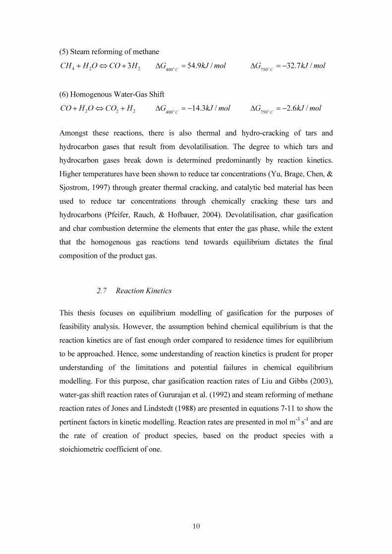
Figure 1: Diagram of FICFB gasifier ............................................................. 13 Figure 2: Siphon.............................................................................................. 14 Figure 3: Page Macrae Updraft Gasifier ........................................................ 15 Figure 4: FICFB Gasifier Model Diagram..................................................... 19 Figure 5: Equilibrium Carbon Distribution for Highvale Coal. Air Ratio = 0.................................................................................... 26 Figure 6: Equilibrium Carbon Distribution for Highvale Coal. Air Ratio = 0.4................................................................................. 26 Figure 7: Equilibrium Carbon Distribution for Highvale Coal. Air ratio = 0.6 .................................................................................. 27 Figure 8: Carbon Formation Boundary. ......................................................... 31 Figure 9: Carbon Formation Boundary (X. Li, Grace, Watkinson, Lim, & Ergudenler, 2001) ................... 32 Figure 10: Ternary Diagram of Elemental Distribution from Steam Gasification of Wood Chips ................................................ 32 Figure 11: Effect of Steam Ratio at 700°C ...................................................... 33 Figure 12: Effect of Steam Ratio at 900°C ...................................................... 33 Figure 13: Fate of Elements at Equilibrium at 700°C ..................................... 36 Figure 14: Fate of Elements at Equilibrium at 800°C ..................................... 37 Figure 15: Fate of Elements at Equilibrium at 900°C ..................................... 38 Figure 16: Effect of Temperature (Steam Ratio = 0.3).................................... 39 Figure 17: Effect of Temperature (Steam ratio = 1) ........................................ 40 Figure 18: Product Gas Composition against Moisture Content (800°C)....... 41 Figure 19: The Effect of Moisture Content on Chemical Efficiency (800°C) 41 Figure 20: Chemical Efficiency and Product Gas Composition against Moisture Content ................................................................ 42 Figure 21: Lower Heating Value of Gases Produced per kmol of Carbon in the System...................................................................... 44 Figure 22: Lower Heating Value of Product Gas (MJ/kmol of gas) ............... 45 Figure 23: Effect of Removing Char from the Reaction System (T=800˚K) .47 Figure 24: Efficiency of a Gasifier against Steam Ratio ................................. 49 Figure 25: Dry Product Gas Composition Trend with Temperature (Steam Ratio = 0.5kg/kg)................................................................ 53 Figure 26: Dry Product Gas Composition Trends with Steam Ratio (T=875˚C)53 Figure 27: Page Macrae Dry Gas Composition for 3rd of August, 2006 ....... 54 Figure 28: Modified Equilibrium Schematic ................................................... 57 Figure 29: Rotary Cascade Drier (Brammer & Bridgwater, 1999)................. 60 Figure 30: Capital Cost and Efficiency of Gas Turbines (Gas Turbine World, 2005)............................................................. 64 Figure 31: IGCC Producer Gas Heating Values .............................................. 66 Figure 32: BIGCC Process ............................................................................... 71 Figure 33: Gasifier-Gas Turbine Process ......................................................... 72 Figure 34: Gasifier-Gas Engine Process .......................................................... 73 Figure 35: Gasifier-Gas Boiler System ............................................................ 74 Figure 36: Gasification Software Model.......................................................... 75

vii

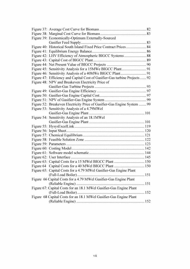
Figure 37: Average Cost Curve for Biomass ................................................... 82 Figure 38: Marginal Cost Curve for Biomass.................................................. 83 Figure 39: Economically-Optimum Externally-Sourced Gasifier Feed Supply....................................................................... 83 Figure 40: Historical South Island Fixed Price Contract Prices...................... 84 Figure 41: Equilibrium Energy Balance........................................................... 86 Figure 42: LHV Efficiency of Atmospheric BIGCC Systems ........................ 88 Figure 43: Capital Cost of BIGCC Plant.......................................................... 89 Figure 44: Net Present Value of BIGCC Projects ........................................... 90 Figure 45: Sensitivity Analysis for a 15MWe BIGCC Plant........................... 91 Figure 46: Sensitivity Analysis of a 40MWe BIGCC Plant............................ 91 Figure 47: Efficiency and Capital Cost of Gasifier-Gas turbine Projects ....... 92 Figure 48: NPV and Breakeven Electricity Price of Gasifier-Gas Turbine Projects ........................................................ 93 Figure 49: Gasifier-Gas Engine Efficiency...................................................... 97 Figure 50: Gasifier-Gas Engine Capital Cost................................................... 97 Figure 51: NPV of Gasifier-Gas Engine System ............................................. 99 Figure 52: Breakeven Electricity Price of Gasifier-Gas Engine System ........ 99 Figure 53: Sensitivity Analysis of a 4.79MWel Gasifier-Gas Engine Plant ............................................................101 Figure 54: Sensitivity Analysis of an 18.1MWel Gasifier-Gas Engine Plant ............................................................101 Figure 55: HysysExcelLink ............................................................................119 Figure 56: Input Sheet.....................................................................................120 Figure 57: Chemical Equilibrium...................................................................121 Figure 58: Feasible Solution Zone .................................................................122 Figure 59: Parameters .....................................................................................123 Figure 60: Costing Model...............................................................................142 Figure 61: Software model schematic ............................................................144 Figure 62: User Interface ................................................................................145 Figure 63: Capital Costs for a 15 MWel BIGCC Plant .................................150 Figure 64 Capital Costs for a 40 MWel BIGCC Plant .................................150 Figure 65: Capital Costs for a 4.79 MWel Gasifier-Gas Engine Plant (Full-Load Boiler) .........................................................................151 Figure 66 Capital Costs for a 4.79 MWel Gasifier-Gas Engine Plant (Reliable Engine) ..........................................................................151 Figure 67: Capital Costs for an 18.1 MWel Gasifier-Gas Engine Plant (Full-Load Boiler) .........................................................................152 Figure 68 Capital Costs for an 18.1 MWel Gasifier-Gas Engine Plant (Reliable Engine) ..........................................................................152

viii

List of Tables

Table 1: Comparison of FICFB and Updraft Gasification.........................17 Table 2: Pinus Radiata Wood Chips (For full analysis see Appendix A1) ............................................20 Table 3: Highvale Coal Ultimate Analysis (wt% as received) ..................25 Table 4: HYSYS Comparison....................................................................28 Table 5: Stoichiometric compared with non-stoichiometric equilibrium ..29 Table 6: Pinus Radiata Wood Chips (For full analysis see Appendix A.1) ...........................................30 Table 7: CAPE FICFB Gasifier Product Gas Composition (mol basis) ....43 Table 8: Comparison of Page Macrae Results with Equilibrium...............43 Table 9: Modified Equilibrium ..................................................................43 Table 10: Design Velocities for FICFB gasifier ..........................................43 Table 11: Gasifier Cost Breakdown.............................................................43 Table 12: Installation Factors for the Gasifier (Ulrich & Vasudevan, 2005)........................................................43 Table 13: Required Gas Quality for Gas Engines and Turbines (Scharpf & Carrington, 2005) ......................................................43 Table 14: Gas Turbine Operating Parameters (Traverso, Cazzola, & Lagorio, 2004) .........................................43 Table 15: Modifications required to Gas Turbine........................................43 Table 16: Steam Cycle Operating Parameters (Energy for Industry, 2005) .........................................................43 Table 17: Energy Balance for a Jenbacher JMS 620 Engine (GE, 2006) ....43 Table 18: GE Jenbacher Gas Engine Costs and Power Outputs (Herdin, 2006)..............................................................................43 Table 19: Capital Cost Parameters...............................................................43 Table 20: Capital Cost Estimating Relationships ........................................43 Table 21: Process Parameters ......................................................................43 Table 22: MDF Plant Energy demands........................................................43 Table 23: Estimated cost of new generation by fuel in the period from 2005 to 2025 ............................................................43 Table 24: Equilibrium Product Gas Composition........................................43 Table 25: Heat Only Process Comparison ...................................................43 Table 26: Comparison of Gasification Electricity Costs with substitutes ...43 Table 27: HYSYS Gibbs Energy parameters...............................................43 Table 28: Equilibrium Compositions from Non-stoichiometric and Stoichiometric Models ..........................................................43 Table 29: CAPE FICFB Results ..................................................................43 Table 30: Chemical Engineering Plant Cost Index (Chemical Engineering) ...............................................................43 Table 31: Exchange Rates............................................................................43 Table 32: Cost driving parameters ...............................................................43 Table 33: Capital Costs for a BIGCC Plant .................................................43 Table 34: Capital Costs for a 4.79 MWel Gasifier-Gas Engine Plant .........43 Table 35: Capital Costs for an 18.1 MWel Gasifier-Gas Engine Plant .......43

ix

Glossary

BFB Bubbling fluid bed. The gasification column of a FICFB gasifier BIGAS Biomass Integrated Gasification Application Systems. The

research consortium within which this thesis was undertaken. BIGCC Biomass Integrated Gasification Combined Cycle C Elemental carbon CH4 Methane CO Carbon Monoxide CO2 Carbon Dioxide C2H4 Ethene or Ethylene CAPE Chemical and Processing Engineering Department of the

University of Canterbury. CFB Circulating fluid bed. The combustion column of a FICFB gasifier. FICFB Fast Internally Circulating Fluidised Bed. The gasifier design used

at CAPE and at Gussing. GCV Gross Calorific Value, equivalent to higher heating value GT Gas Turbine H Elemental hydrogen H2 Diatomic hydrogen HHV Higher Heating Value HRSG Heat Recovery Steam Generator IGCC Integrated Gasification Combined Cycle, typically fuelled with

coal but also refinery coke. LHV Lower Heating Value MED Ministry of Economic Development N Elemental nitrogen N2 Diatomic nitrogen NM3 Normal meter cubed. A unit of volume representing a meter cubed

at standard conditions. O Elemental oxygen OD basis Oven Dry Basis S Elemental sulphur Steam Ratio Ratio of steam and moisture into the gasifier to dry wood feed. NOTE: All dollars are 2005 NZ$ unless otherwise stated. Where dated cost correlations are used the Chemical Engineering Plant Cost Index (see Appendix B.5) has been used to account for inflation.

1

1 Introduction

Economic growth and increased energy demand have historically been intertwined. As New Zealand grows and so does its demand for energy. Estimates for the electricity demand range from 1.2% p.a between 2000 and 2025 (A. Smith et al., 2003) to 2.7% p.a (Electricity Commission, 2006). At the conservative rate of growth 3,355 MW of new generation will have to be built in the next 25 years. This is equivalent to 37.8% of New Zealand’s current generation capacity and is greater than New Zealand’s current thermal generation capacity (Dang, 2005). However, traditional sources of electricity generation have largely been tapped. Large scale hydro, greater than 75 MWel, currently makes up more than 50% of New Zealand’s generation mix, but the demise of Project Aqua is seen by many as the end of large scale hydro development in New Zealand. Gas-fired electricity currently makes up 20% of New Zealand’s total generation capacity (Dang, 2005) but future sources of natural gas are uncertain due to the depletion of the Maui gas field. Because of this, New Zealand will have to look for other sources of energy to meet its growing energy demand. Furthermore, the majority of New Zealand’s energy resources are situated distant from the demand centres. For instance, the majority of New Zealand’s coal resource is found in Southland. Building more generation remote from the demand centres increases the pressure on an already ageing and increasingly constrained transmission network. The backbone of New Zealand’s transmission network was built in the 1950s and 1960s and Transpower (2004) estimates $1.5B will need to be invested in the grid in the near future. Cogeneration, the generation of electricity in situations where there is a consumer for the waste heat, can play a role in mitigating both issues expressed above. Cogeneration plant is situated alongside major energy users, therefore, reducing or eliminating the need for transportation of the energy. Furthermore, cogeneration can enable the economic use of a number of fuels, which have not previously been tapped to their full potential.

2

Biomass, and wood in particular, offers an ideal cogeneration fuel. It is a renewable, carbon neutral1 resource which is abundant in New Zealand. The Ministry of Agriculture and Forestry (2004) reports that New Zealand has 1,822,000 ha of managed commercial forest from which 20 million m3 of round-wood is harvested annually (Pang, 2005). Harvesting this round-wood results in around 4 million m3/yr of waste residues and processing results in a further 4.5 million m3/yr in waste residues (Pang, 2005). The majority of the harvest residue is left on the forest floor to rot and the process residue is, at best, used in combustion processes to provide heat to the processing plant. Conservatively, these waste residues offer 33 GW of thermal energy and, if integrated with cogeneration gasification (~30% electrical efficiencies), could offer installed capacity of the same order as New Zealand’s total installed capacity as of 2005. Now it will not be economical or feasible to utilize the wood resource to this potential, but the point is that the wood resource is there and for the forest products industries, which are energy-intensive industries, it provides a strategic energy resource. The wood products industries (predominantly sawmilling and timber dressing) and the pulp and paper industry each consume 5% of the total amount of electricity produced in New Zealand each year . Biomass gasification offers an appealing cogeneration process for the energy intensive wood industry. The appeal of biomass gasification stems from the fact that gasification transforms a solid, often waste, fuel into a gaseous fuel which retains 75-88% of the heating value of the original (Higman & Burgt, 2003). A gaseous fuel offers easier handling and the ability to utilize either a gas engine or a gas turbine, giving far more versatility in the options for integration of biomass into combined heat and power (CHP) plants. Gas turbines offer significant thermodynamic efficiency gains over combustion steam cycles due to the greater temperatures obtainable in gas turbine cycles. Steam power cycles are limited to a maximum steam temperature of around 480˚C due to the metallurgy of the steam superheaters (Franco & Giannini, 2005), while the maximum temperature in gas turbine cycles is around 1400-1600˚C and limited by the metallurgy of gas turbine blades (Rodrigues, Faaij, & Walter, 2003). This allows biomass gasification combined cycles to operate with electrical conversion 1 The carbon emitted during combustion of wood is equal to the carbon sequestered during the growth of the tree.

Therefore the net emission of carbon is zero.

3

efficiencies of 35-40% opposed to efficiencies of 15-28% for the conventional biomass steam turbine cycles (Franco & Giannini, 2005). New Zealand is being forced to look for new generation options in an environment of a constrained electricity grid. In this environment, an economically viable, carbon-neutral, renewable, indigenous cogeneration energy option would go far to help in securing New Zealand’s energy future. This thesis aims to answer whether biomass gasification is this energy option. This is done by presenting an economic feasibility assessment of the application of gasification in a cogeneration role with a medium density fibreboard (MDF) plant. This thesis contains:

• a literature review of key gasification concepts, o The literature review introduces gasification and presents a rationale for

the approach taken to gasification modelling • an introduction and discussion of gasification modelling,

o Gasification modelling is a major part of this thesis and includes creating and testing a model capable of predicting the product gas composition from gasification

• a review of gasification process equipment, o The introduction to gasification process equipment introduces the major

equipment items and some of the challenges in using them • an introduction and discussion of economic modelling,

o The economic modelling presents a cash flow analysis for four of the most appealing gasification processes

• conclusions on the economic feasibility of biomass gasification.

4

2 Gasification

2.1 The BIGAS Consortium

“The conversion of any carbonaceous fuel to a gaseous product with a heating value” (Higman & Burgt, 2003)

Gasification is the thermal decomposition of fuel, in this case wood, into gases with a heating value. Thereby, it offers a technology that allows the utilization of solid wood in today’s high efficiency power generation technologies such as gas turbines and gas engines. Research in gasification, as an enabling technology for encouraging cogeneration, is the focus of the Biomass Integrated Gasification Application Systems (BIGAS) consortium. The consortium has partners both in academia and in industry, with involvement from the University of Canterbury, University of Otago, Delta S Technologies, Meridian Solutions, Page Macrae and Selwyn Plantation Board. The consortium is structured into four objectives listed below:

• Objective 1: Evaluate the current state of gasification technology and recommend a gasification technology best suited for development in New Zealand.

• Objective 2: Technical development of the selected gasification technology. • Objective 3: Quantify availability and cost of wood fuel and quantify energy

demand in the wood processing sector. • Objective 4: Develop a model for the selected technology for use in the design

of a pilot gasification plant and develop economic feasibility studies for this technology.

Objective one recommended Fast Internal Circulating Fluidized Bed Technology (FICFB) developed by the University of Vienna and a 100 kWth FICFB gasifier has been built at the Chemical and Process Engineering Department (CAPE) at University

5

of Canterbury. In conjunction with this, Page Macrae is developing an updraft gasifier and has a 1.7 MWth gasifier currently in operation. This thesis represents the work to date undertaken to achieve objective four of the consortium. There are two final outputs of this objective. The first is a gasification modelling tool for aiding in the design of a gasification pilot plant and the second is a software model of FICFB cogeneration systems that allows foresters, wood processors and other investors to evaluate the feasibility of an integrated gasification energy plant. This thesis has been successful in providing a gasification modelling tool based on chemical equilibrium, which can be applied to both FICFB gasification and updraft gasification, and in providing a software model for the economic feasibility of FICFB gasification integrated with an MDF plant. This software model is restricted to MDF plants, as data from objective three is not yet available for other processing plants. The model is also restricted to FICFB gasification, as this concept has been proven to produce a gas more suited to power generation. Updraft gasification systems, on the other hand, are known to produce a gas with a significant tar content and are, therefore, more suited to heat-only applications. Furthermore, because the Page Macrae updraft gasification system is being developed by private enterprise, information about the cost of it is commercially sensitive. This thesis can be separated into two sections; gasification modelling and feasibility modelling. The following section is a literature review for gasification modelling. It introduces the basic concepts of gasification and builds a case for taking the chemical equilibrium modelling approach. Section 8 represents the start of the feasibility modelling and presents a literature review which introduces the process units required for gasification cogeneration and presents a rationale for the validity of the chosen processes. Note: Detailed discussion about the CAPE FICFB gasifier, the testing methodology and the current (as of October 2006) FICFB results are part of objective two’s work programme. If interested, the reader should refer to the work by Brown, Dobbs and Gilmore (2006).

6

2.2 Introduction to Gasification Reactions

Carbonaceous fuel undergoes five types of chemical conversions in a gasifier; drying, devolatilisation, char gasification, combustion (in localized areas of excess oxygen) and homogenous gas-phase reactions. Drying relates to the release of moisture from the fuel. Devolatilisation is a very complex reaction set with many intermediate products but can be considered simply as the reaction of dry biomass into light gases, tar and char. The tars can be thermally or catalytically cracked to smaller tars or light gases. The char either undergoes char gasification reactions or char combustion reactions. The resulting gas from devolatilisation, char gasification and char combustion rise and undergo homogenous gas phase reactions.

2.3 Drying

Drying is the release of moisture from the biomass. Wet Biomass ↔ Dry Biomass + Water Vapour (CH1.44O0.66 + H2O(l)) ↔ CH1.44 O0.66 + H2O(v)

2.4 Devolatilisation

Devolatilisation is the thermal decomposition of the biomass and takes place at temperatures between 350˚C and 800˚C (Higman & Burgt, 2003). The literature frequently reports devolatilisation as a multi-stage process beginning with the decomposition of the biomass into light gases (primarily H2O, H2, CO, CO2 and CH4

but also some higher hydrocarbons), tar and char (Babu & Chaurasia, 2003; Corella & Sanz, 2005; Higman & Burgt, 2003; Koufopanos, Papayannakos, Maschio, & Lucchesi, 1989). Heating rate and temperature have a significant effect on the devolatilisation yield and composition. Other variables, such as the composition of the surrounding atmosphere, have a lesser effect. This leads to many devolatilisation models being independent of the composition of the surrounding atmosphere (de Souza-Santos, 2004). However, because the surrounding atmosphere is not often taken into account, devolatilisation models need to be applied with care, especially to FICFB gasification where a strong hydrogen environment exists. Once devolatilisation has occurred, the gases, tar and char have the opportunity to undergo further chemical reaction. Equation 1, below, shows the products from

7

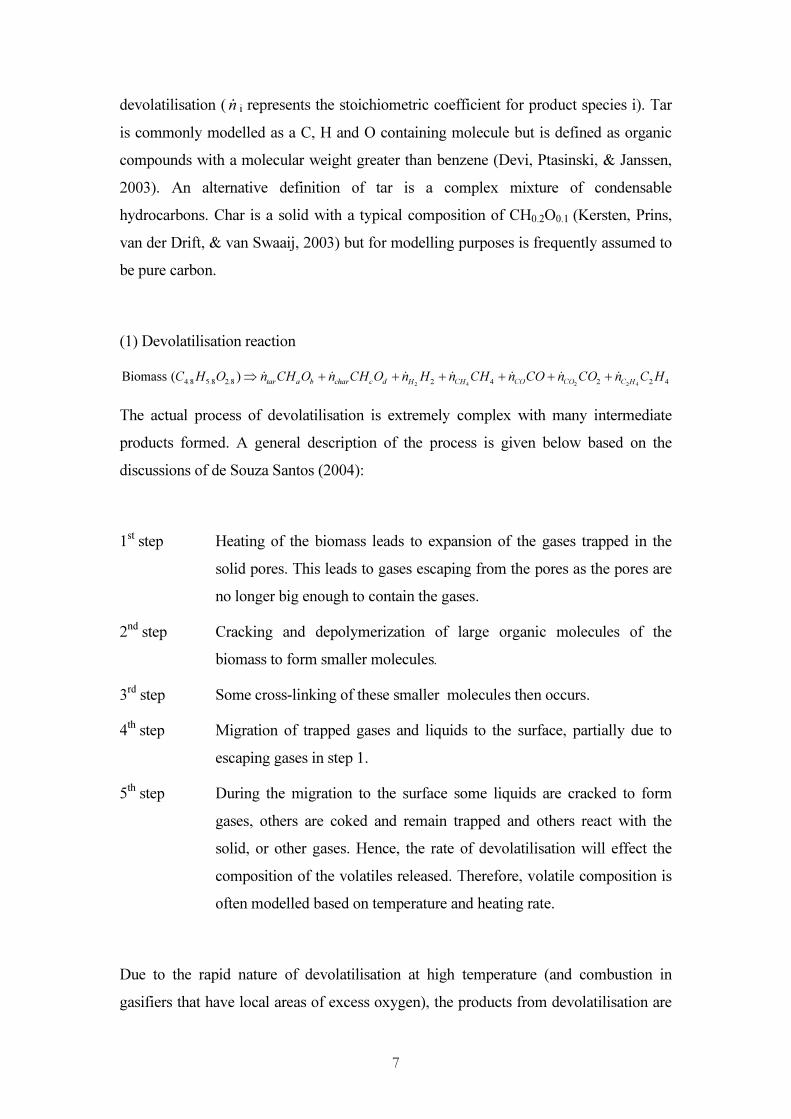
devolatilisation ( n� i represents the stoichiometric coefficient for product species i). Tar is commonly modelled as a C, H and O containing molecule but is defined as organic compounds with a molecular weight greater than benzene (Devi, Ptasinski, & Janssen, 2003). An alternative definition of tar is a complex mixture of condensable hydrocarbons. Char is a solid with a typical composition of CH0.2O0.1 (Kersten, Prins, van der Drift, & van Swaaij, 2003) but for modelling purposes is frequently assumed to be pure carbon. (1) Devolatilisation reaction

2 4 2 2 44.8 5.8 2.8 2 4 2 2 4Biomass ( ) tar a b char c d H CH CO CO C HC H O n CH O n CH O n H n CH n CO n CO n C H⇒ + + + + + +� � � � � � �

The actual process of devolatilisation is extremely complex with many intermediate products formed. A general description of the process is given below based on the discussions of de Souza Santos (2004): 1st step Heating of the biomass leads to expansion of the gases trapped in the

solid pores. This leads to gases escaping from the pores as the pores are no longer big enough to contain the gases.

2nd step Cracking and depolymerization of large organic molecules of the biomass to form smaller molecules.

3rd step Some cross-linking of these smaller molecules then occurs. 4th step Migration of trapped gases and liquids to the surface, partially due to

escaping gases in step 1. 5th step During the migration to the surface some liquids are cracked to form

gases, others are coked and remain trapped and others react with the solid, or other gases. Hence, the rate of devolatilisation will effect the composition of the volatiles released. Therefore, volatile composition is often modelled based on temperature and heating rate.

Due to the rapid nature of devolatilisation at high temperature (and combustion in gasifiers that have local areas of excess oxygen), the products from devolatilisation are

8

often used as a starting point for gas composition in kinetic models of fluid-bed gasification processes (Corella & Sanz, 2005; Kaiser et al., 2000; Kinoshita & Wang, 1993). These fluid-bed gasification models begin with composition and yields of product gas, tar and char as dictated by fast pyrolysis (devolatilisation with a heating rate greater than 103 K/s) reactions and then develop reaction rates to describe how far the composition goes towards an equilibrium composition. Unfortunately, there is limited data on the compositions and yields of fast pyrolysis from biomass at temperatures above 700°C and this data tends to be gasifier specific (Yu, Brage, Chen, & Sjostrom, 1997). Such an approach cannot be taken with updraft gasification as the fuel enters the gasifier in a region of moderate temperature (350 to 500°C) and, hence, dries and devolatilises at a slower rate.

2.5 Char Gasification Reactions

The gasification reactions occur simultaneously to the drying and devolatilisation reactions. Char gasification reaction rates are many orders of magnitude slower than the drying and devolatilisation reactions (Bilodeau, Therien, Proulx, Czernik, & Chornet, 1993) and, therefore, the extent to which they take place governs the carbon conversion rate (Higman & Burgt, 2003). These reactions transform the char and tar, which are products of the devolatilisation reactions, and release further light gases. Unlike devolatilisation and drying, which occur immediately and, therefore, close to the feed entry point, char gasification is likely to occur throughout the bed. The major char gasification reactions are shown in equations 2-4 below. (2) Heterogeneous Water-gas Shift

22)( HCOOHC s +⇔+ 400 39.5 /CG kJ molο∆ = 750 10.8 /CG kJ molο∆ = −

(3) Hydrogenation Gasification

42)( 2 CHHC s ⇔+ 400 15.4 /CG kJ molο∆ = − 750 21.9 /CG kJ molο∆ =

(4) Boudouard Equation COCOC s 22)( ⇔+ 400 53.8 /CG kJ molο∆ = 750 8.2 /CG kJ molο∆ = −

9

In FICFB gasification, there may not be significant char gasification as Kersten et al. (2003) suggest that the residence times in atmospheric CFB biomass gasifiers at temperatures of 700-1000˚C are not sufficient for the char gasification reactions to proceed to a significant extent. Furthermore, there is evidence that H2O and CO2 gasification of char are inhibited by the presence of CO and H2 (Gururajan, Agarwal, & Agnew, 1992). However, the rate of char gasification can be increased through catalytic reactions with Ca, K or Na (Gururajan, Agarwal, & Agnew, 1992). Miura, Hashimoto et al. (1989) experiments on coal chars found that the reactivity of high rank coals is determined predominantly by total surface area but the reactivity of low rank coals (less than 80%wt carbon) is primarily determined by catalytic active metals (Ca, Fe, Na and K). Woody biomass has a carbon content of around 50% wt O.D basis (See Appendix A.1 and A.12) and, therefore, catalysis of the biomass char will be important in encouraging char gasification reactions. Char gasification reactions are slow. They are the limiting factor in carbon conversion (Bridgwater, 1995) and may not, in fact, occur to a significant extent (Kersten, Prins, van der Drift, & van Swaaij, 2003). This suggests that the major mechanisms for carbon entering the gas phase are devolatilisation and char combustion, rather than char gasification. This has consequences for FICFB reactors where char combustion is confined to a separate combustion zone, leaving devolatilisation as the primary mechanism for converting carbon into the gas phase. Hence, the amount of volatiles in the biomass is likely to be a significant factor in FICFB gasification.

2.6 Homogenous Gas Phase Reactions

The water-gas shift reaction and the steam reforming of methane reaction (equations 5 and 6) are the most common reactions used to describe any changes in composition of the product gases as they rise through the bed and freeboard.

10

(5) Steam reforming of methane 224 3HCOOHCH +⇔+ 400 54.9 /CG kJ molο∆ = 750 32.7 /CG kJ molο∆ = −

(6) Homogenous Water-Gas Shift

222 HCOOHCO +⇔+ 400 14.3 /CG kJ molο∆ = − 750 2.6 /CG kJ molο∆ = − Amongst these reactions, there is also thermal and hydro-cracking of tars and hydrocarbon gases that result from devolatilisation. The degree to which tars and hydrocarbon gases break down is determined predominantly by reaction kinetics. Higher temperatures have been shown to reduce tar concentrations (Yu, Brage, Chen, & Sjostrom, 1997) through greater thermal cracking, and catalytic bed material has been used to reduce tar concentrations through chemically cracking these tars and hydrocarbons (Pfeifer, Rauch, & Hofbauer, 2004). Devolatilisation, char gasification and char combustion determine the elements that enter the gas phase, while the extent that the homogenous gas reactions tend towards equilibrium dictates the final composition of the product gas.

2.7 Reaction Kinetics

This thesis focuses on equilibrium modelling of gasification for the purposes of feasibility analysis. However, the assumption behind chemical equilibrium is that the reaction kinetics are of fast enough order compared to residence times for equilibrium to be approached. Hence, some understanding of reaction kinetics is prudent for proper understanding of the limitations and potential failures in chemical equilibrium modelling. For this purpose, char gasification reaction rates of Liu and Gibbs (2003), water-gas shift reaction rates of Gururajan et al. (1992) and steam reforming of methane reaction rates of Jones and Lindstedt (1988) are presented in equations 7-11 to show the pertinent factors in kinetic modelling. Reaction rates are presented in mol m-3 s-1 and are the rate of creation of product species, based on the product species with a stoichiometric coefficient of one.

11

(7)

(8)

(9)

0pρ is the initial density of char (kg/m3). Fiaschi and Michelini (2001) state this as 1500 bW is the initial mass fraction of carbon in the char. Corella and Sanz (2005) present

char as CH0.2O0.1 giving a mass fraction of 0.87 0f is a reactivity factor of 10 for biomass chars (Liu & Gibbs, 2003) charε is void fraction of the char ( )F x ~ 0.4 pT is the temperature of the char particle

[ ]i is the concentration of the species i (kmol/m3 of gas) (10) (11) Based on equations 7-11, gasification reaction rates are a function of char density, mass fraction of carbon in char, char reactivity, void fraction in char, temperature of the char particles and concentration of the gaseous species. Other common influencing factors are particle size, size distribution, char pre-treatment and mineral content of the char (Liliedahl & Sjostrom, 1997). Hence, reaction rate models tend to be very specific and have limited general applicability.

2 2

2

2 4

15,5165

23728 7196 11559

2 3 52 2

32,23510

22 3067

2 12

2

2.39 10 e [ ]=k 1 3.16 10 [ ] 5.36 10 [ ] 8.25 10 [ ]

4.89 10 e [ ]=k 1 6.6 10 [ ] 1.2 10 [ ]

0.0239 1=k

p

p p p

p

p

T

C H O CO HT T T

T

C CO COT

C H CH

H ORe H O e H e CO

CORCO e CO

R

−

+ ⇔ +

− − −

−

+ ⇔

− −

+ ⇔

××

+ × + × + ×

××

+ × + ×

××

15,5165

23728 7196 11559

2 3 52 2

00

0 e [ ]

1 3.16 10 [ ] 5.36 10 [ ] 8.25 10 [ ]

k ( )12

p

p p p

T

T T T

char b char

H

e H O e H e COW fwhere F xρ ε

−

− − −+ × + × + ×

=

( )2 2

2 2 2 2

1510.7 3958.51

1 ,2,

2780 and 0.0265CO H RT TCO H CO H O CO H O wg equilibrium

wg equilibirum

P PkR P P where k e K eKRT

− + ⇔ +

= − = =

4 2 2

15,0988

3 4 23.0 10 [ ][ ]TCH H O CO HR e CH H O

−

+ ⇔ + = ×

12

2.8 Chemical Equilibrium

Chemical equilibrium, on the other hand, is based purely on thermodynamic state properties of the gasifier and molar flow of elements into the gasifier. Therefore, these models have a wide applicability. Chemical equilibrium modelling requires the assumption that the residence times of the components is sufficient for chemical equilibrium to be reached. Although chemical equilibrium is never actually realized in a gasification process, equilibrium models have been demonstrated to perform well at high temperatures (1230˚C) (Altafini, Wander, & Barreto, 2003). So well in fact that Higman and Burgt (2003) state that chemical equilibrium forms the basis of most commercial gasification reactor designs. However, Higman and Burgt (2003) do suggest that biomass gasification is an exception to this. The performance of equilibrium models reduces with temperature and at moderate temperatures (<530˚C) these models do not perform well. The two major inconsistencies between equilibrium models and experimental observation are the carbon conversion and the methane yield (X. T. Li et al., 2004). Measured methane yields by Li et al. (2004) were substantially higher due to incomplete cracking of devolatilisation products, and measured carbon conversion was lower due to insufficient residence times.

2.9 Rationale of Modelling Approach

A chemical equilibrium approach has been chosen as this approach has, to the author’s knowledge, not been rigorously applied to FICFB gasification. Chemical equilibrium is appealing as the independence from experimentally derived gasifier-specific data allows the model to be applied to both types of gasifier that exist within the BIGAS consortium. Furthermore, in the context of creating a model for assessing the economic feasibility, the weaknesses of chemical equilibrium were expected to have an insignificant effect on gasification’s overall economic appeal. The FICFB gasifier commissioning at the CAPE took longer than expected and experimental results of product gas composition were not obtained until July, 2006. Therefore, due to the current stage of the gasifier project, the experimental runs required for kinetic modelling would not have been possible. However, the scope for study of reaction kinetics and their importance to FICFB gasification is recognized and, once the gasifier project has matured sufficiently, offers an appealing avenue for further research.

13

3 Primary Types of Gasifier

3.1 Introduction

The BIGAS consortium is involved with the development of two different types of gasifier; the University of Canterbury FICFB gasifier and the Page Macrae updraft gasifier. The two gasifiers have quite different characteristics which are outlined in this section.

3.2 FICFB Gasification

The FICFB gasifier produces a high hydrogen gas yield due to the use of steam as the gasifying agent. The endothermic nature of the gasification reactions combined with the use of steam as a gasifying agent requires some heat transfer to the gasification reactor. This is achieved through a twin bed system. The bubbling fluid bed (BFB) gasification reactor is combined with a circulating fluid bed (CFB) combustor. The CFB heats an inert heat carrying medium (sand) which flows from the CFB to the BFB providing the heat of reaction. A diagram of the system is shown in Figure 1, below.

2SteamN H O�

BFB Gasification Biomass &

Nitrogen Gas

Product Gas

SteamCool Sand& Char

CFBCombustion

Hot Sand

Flue Gas

Air

LPG2SteamN H O�

BFB Gasification Biomass &

Nitrogen Gas

Product Gas

SteamCool Sand& Char

CFBCombustion

Hot Sand

Flue Gas

Air

LPG

Figure 1: Diagram of FICFB gasifier

14

The BFB reactor is screw-fed biomass accompanied by a nitrogen purge gas. The nitrogen purge gas is used to ensure positive gas flow into the gasifier, hence, reducing the risk of fire in the feed hopper or release of product gas through the feed system. The biomass is fed in above the fluid bed. Drying and devolatilisation of the biomass occur immediately upon the biomass entering the reactor. The gasification reactions, particularly heterogeneous char-gasification reactions, have longer reaction rates and may occur throughout the BFB. The BFB is a sand bed fluidized with steam. Depending on the gasification operating conditions, the bed may also contain significant amounts of char. The sand and char bed material flows from the BFB through a chute fluidized with either air or steam into the CFB. Inside the CFB, the char and any additional fuel in the form of LPG is combusted. The CFB is a sand bed fluidized with air. Air rates are maintained to provide excess air conditions of between two and five percent. The CFB air velocity is significantly greater than the steam velocity in the BFB (7ms-1 compared to 1.5ms-1) and hence the sand is entrained up and out of the CFB. The sand entrained out of the CFB is separated from the flue gases by a cyclone and fed back through a siphon into the BFB. The hot sand settles at the bottom of the siphon preventing flow of the BFB product gas through the siphon. The sand is then fluidized with either air or steam up and over into the BFB, as shown in Figure 2 below.

Hot Sand from CFB

Hot Sand into BFB

S i p h o n F l u i d i s i n g G a s

Figure 2: Siphon

The sand, having passed through the combustion reactor, is hotter than the BFB bed and cools providing the heat for the gasification reactions. The product gas from the BFB

15

flows out of the top of the BFB and through a cyclone to separate particulates before being burnt in an afterburner. When the FICFB is integrated into a process the afterburner would be replaced with a boiler system, a gas engine or a gas turbine as shown in the process flow sheets of section 8.2, and LPG would be replaced with re-circulated product gas.

3.3 Updraft Gasification

Updraft gasification processes use either air or oxygen (the Page Macrae system uses air) as the gasification agent, allowing combustion inside the gasification reactor and removing the need to supply heat through a secondary combustion column. Hence, updraft gasifiers consist of one reactor column. Air or oxygen is supplied to the bottom of the reactor and wood chips are screw-fed in near the top. As in FICFB gasification, drying and devolatilisation take place as the fuel enters the reactor. However, unlike FICFB gasification, there is not a fluid bed to remove the char and tar. This results in a stationary matrix of char forming inside the reactor. Wood feed rates are generally controlled to maintain stationary bed heights. A water slurry and a mechanical grate at the bottom of the reactor are used to remove ash. The Page Macrae system is shown in Figure 3.

Figure 3: Page Macrae Updraft Gasifier

16

Due to air or oxygen being used as the gasification agent, combustion occurs in the bed. This provides the heat for the endothermic gasification reactions and provides another pathway for getting elements into the gas phase. It also results in a hot region around the entry point of the oxidant. The region above the combustion region is where the char gasification reactions occur as hot combustion gases mix with the char matrix. Above the gasification region, drying and devolatilisation of the incoming feed occur. This results in a temperature profile which is hottest at the entry point of the oxidant and decreases with height. Because of this, tars formed from devolatilisation do not undergo thermal cracking and the resulting product gas generally has a high tar content (Coulter, 2005). In cases where air is used instead of oxygen, the product gas is diluted significantly by the presence of nitrogen. This can dilute the product gas by a factor of two and is the major driver for the use of oxygen as a gasification agent. The Page Macrae system is designed to be coupled with a boiler for the provision of heat. Its advantages over wood combustion systems are that a smaller mechanical grate is required - the Page Macrae gasifier generates 2 MWth/m2 of grate area whereas a typical wood combustion grate manages only 650kWth/m2 (Coulter, 2005) - and emissions are significantly below regulatory boundaries. The Page Macrae system emits 12 mg/NM3 of particulates (Coulter, 2005). The limit for emissions in the Canterbury region for solid fuel burners greater than 40kW is 250 mg/NM3, and 50 mg/NM3 regulations are being adopted by some councils (Fisher et al., 2005).

17

3.4 Comparison of the Two Systems

The FICFB system is designed to deliver a medium calorific value fuel with high hydrogen content, while the Page Macrae system produces a low calorific value fuel. The CAPE system is designed to be utilized with either a gas engine or gas turbine for the provision of heat and power, while the Page Macrae system is designed purely for heat provision. The CAPE FICFB system is more complicated and, for similar scale, more expensive. A summary of the differences between the two systems is given in Table 1.

Table 1: Comparison of FICFB and Updraft Gasification CAPE FICFB Page Macrae Up-draft

Product Gas Composition (Dry Mol Fractions)

CH4 H2 CO CO2 C2H4 C2H6 N2

10-12% 18-21% 26-30% 17-18% 3-4% 1%

14-25%1

1.5-3% 9.5-20% 10-20% 14-20% 0-0.5% 0-0.2% 43-50%

Lower Heating Value (MJ/NM3Dry) 10.8-12.9 2.7-6.0 Water Content (vol/vol) 20% 30% Gas Outlet Temp (˚C) 700-900 350-500

Tar Content Medium High Fluidizing Agent Steam Air

Number of reactors Two One Scale (kWth) 100 1700

1 The high levels of nitrogen are caused because the CAPE gasifier currently runs with air fluidizing the chute and siphon. When steam is used to fluidize the chute and siphon this should drop to around 5% (achieved in the University of Vienna pilot plants) and result purely from nitrogen purge and fuel nitrogen.

18

4 Gasifier Modelling Method

4.1 Introduction

Modelling of the gasification process has been undertaken in order to provide information about the heating value and product gas yield so as to allow feasibility studies on gasification energy plants. With this goal, a chemical equilibrium approach to modelling gas composition exiting the gasifier was chosen. Chemical equilibrium offers an appealing approach as it is insensitive to gasifier specific parameters. Temperature and elemental abundances are the only required inputs for chemical equilibrium. This allows the creation of a gasifier model which has a wide applicability. However, as the gasifier characteristics which affect reaction rate are not taken into account, such a model cannot predict how closely the product gas composition will mirror equilibrium. With this is mind, a chemical equilibrium model has been presented to show the thermodynamic limits of gasification, the effect of modifying different gasification parameters and the degree of separation between experimental product gas compositions and equilibrium compositions.

4.2 Description of Model

Chemical equilibrium gives a black box model. This means that the internal workings of the gasifier are not considered. No information is given on temperature or concentration profiles inside the gasifier but, given information on the elemental flows into the gasifier and the temperature of the gasifier, the composition of the product gas can be derived. The gasification reactor has a known amount of carbon, hydrogen, oxygen and nitrogen entering it. This can be in any form. Equilibrium composition is insensitive to the state or the species in which the elements enter the reactor. However, the state and species will affect the heat of reaction and, hence, the energy demand of the gasification reactor. If char circulation for FICFB gasification is specified, then this carbon is removed from the equilibrium calculation. Inside the gasification reactor, mixing and residence times are assumed to be sufficient for the system to reach equilibrium before the product gas exits. The reactor is at a specified uniform temperature and the product gas exits at the equilibrium composition for that temperature.

19

Modelling of FICFB gasification is taken a step further and a complete energy balance is undertaken so that either char circulation (where there is no re-circulated product gas) or the amount of re-circulated product gas can be calculated. For FICFB gasification, heat is supplied to maintain the uniform temperature in the reactor via the circulation of sand from the CFB section. Sand circulation is calculated to meet the heat of reaction as well as specified heat loss from the system. The specified char circulation is completely combusted in a CFB reactor. A portion of the product gas is re-circulated to the CFB to maintain the energy balance. The temperature of the CFB is specified and is a trade-off between fuel requirements and sand circulation rate. In practice, it will be set as low as the sand circulation rate will allow. Figure 4 illustrates the flows present in FICFB gasification.

Figure 4: FICFB Gasifier Model Diagram The reacting system in the gasification reactor has been assumed to be only carbon, hydrogen and oxygen. Nitrogen has been included in the model as a non-reacting element. This is a reasonable representation of reality as N2 is highly inert and the wood feed only contains trace amounts of other elements (see Table 2). It is known that minerals in the ash have catalytic properties and are, therefore, important. However, the presence of these materials will only aid in the composition reacting further towards equilibrium and will not change the equilibrium composition.

CFB

BFB

Wood Feed (CHxOy), Moisture and

Nitrogen Purge

Product Gas

Flue Gas

Air Product Gas

Char and Sand

Sand

Steam

20

Table 2: Pinus Radiata Wood Chips (For full analysis see Appendix A.1) Dry Moisture GCV

(Dry) Pinus Radiata Chips C H O S N Ash As.

Received MJ/kg Wt.% 51.2 6.1 42.3 0.02 <0.2 0.04 52.6 20.1 Mol.% 30.5 44.9 24.5 0 0 -- -- --

Mol Ratio 1 1.47 0.80 -- -- -- -- -- CO, CO2, CH4, H2O, H2 and N2 are the major products of gasification. Typical gasification temperatures are high enough that hydrocarbons heavier than methane exist only in small quantities (Higman & Burgt, 2003) and if the gasifier is operating at equilibrium they should not exist at all, as shown in section 6.4. Further discussion and testing of this assumption is presented in section 5.1 Therefore, a model aiming to predict the amount of these species that exist at equilibrium in non-negligible concentrations can be expressed as the seven species equilibrium shown below. Wet Wood + Steam + N2 purge CH4 + CO2 + CO + H2 + H2O + N2 + C(s) The formation of solid carbon can be thought of as saturation of elemental carbon in the gas phase (X. Li, Grace, Watkinson, Lim, & Ergudenler, 2001). Hence, at low temperatures and in high carbon systems, equilibrium will yield solid carbon. At high temperature or in low carbon systems, no solid carbon will form. For further discussion see section 6.2. Elemental balances provide equations for four of the species. Therefore, two additional equilibrium equations are required for non-carbon forming systems and three additional equations are required for carbon forming systems. These extra equations are provided by the water-gas shift reaction and steam-methane reforming reaction in the case of no solid carbon formation and the Boudouard reaction, methanation reaction and heterogeneous water-gas shift reaction for systems which form solid carbon.

21

4.3 Calculated Variables

The following variables are calculated by the model:

is the molar flow out of the BFB of CH4 at equilibrium. is the molar flow out of the BFB of CO at equilibrium. is the molar flow out of the BFB of CO2 at equilibrium. is the molar flow out of the BFB of H2 at equilibrium. is the molar flow out of the BFB of H2O at equilibrium. is the molar flow out of the BFB of N2 at equilibrium. is the molar flow out of the BFB of solid carbon at equilibrium. is the molar flow out of the BFB of product gas at equilibrium.

4.4 Input Parameters

The following parameters are required as inputs into the model: is the molar flow of wood into the system in the form CHyOx is the hydrogen to carbon ratio in the dry wood is the oxygen to carbon ratio in the dry wood. is the molar flow of moisture into the system with the wood. is the molar amount of carbon removed from the equilibrium calculation by char circulation. is the molar flow of steam into the system is the molar flow of nitrogen purge gas is the temperature for calculating equilibrium of the BFB

4CHN

CON

2CON

2HN

OHN2

2NN

)( sCN

gasN

xyOCHN

y

x

MoistureN

CharN

SteamN

2NN

BFBT

22

22422

4

)( HOHmoisturesteamOCHwoodCH

NNNNxNN yx

+−

++=

( )22)(

2)(222 )()( HOHmoisturesteamOCHwoodCcharOCHwoodCO NNNNNyxNNNNyxsyx

+++−

++−−=

( ) 23

2)(3

422

)(2 )()(HOHmoisturesteam

CcharOCHwoodOCHwoodCONNNNNNNNyxN

syxyx

+−++−−−

+=

( ) 23

2)(3

422

2)( )()(HOHmoisturesteam

charOCHwoodOCHwoodCOC

NNNNNNNyxNNyxyxs

+++−−+

+−=

4.5 Model Equations

Four of the calculated variables can be solved through elemental balances for carbon, hydrogen, oxygen and nitrogen. The elemental balances are shown below. (12) Carbon Balance

(13) Hydrogen Balance

(14) Oxygen Balance

(15) Nitrogen Balance Through these equations the molar flows of methane, carbon monoxide and carbon dioxide or solid carbon can be shown to be dependent on the molar flows of product steam and hydrogen, see Appendix A.2 and equations 16-19. The molar flow of nitrogen can be calculated through equation 20. (16)

(17)

(18)

(19)

(20) Equations 18 and 19 are the same and, therefore, cannot be used to find both the yield of carbon dioxide and the yield of solid carbon. Equation 18 is used when no solid carbon is present in the products and Equation 19 is used when there is solid carbon in

PurgeN NN =2

22422422)( HOHCHmoisturesteamOCHwood NNNNNxN

yx++=++

4 2 ( )( )x y swood CH O CH CO CO char CN N N N N N= + + + +

OHCOCOmoisturesteamOCHwood NNNNNyNyx 22

2)( ++=++

2NPurge NN =

23

the products. When there is solid carbon present the yield of the hydrogen, steam and carbon dioxide is found through the assumption of chemical equilibrium. When there is no solid carbon present, the assumption of equilibrium is only needed to find the yield of hydrogen and steam. Chemical equilibrium is used to relate the partial pressures of the species partaking in a chemical reaction to the temperature at which the reaction takes place using equation 21 and 22. (21)

(22)

In order to use equations 21 and 22 to find the mol fraction of the desired species a reaction set which represents the interaction of the species with the remaining constituents of the product gas is needed. Equations 2-4 show a reaction set for the case where solid carbon is a product and equations 5-6 show a reaction set for the case where there is no solid carbon product. (2) Heterogeneous Water-gas Shift

(3) Hydrogenation Gasification

(4) Boudouard Equation

(5) Steam reforming of methane

(6) Homogenous Water-Gas Shift

i0

0

x

Gln -RT

i

i

v

v PkP

k

∑ = ∆=

∑

224 3HCOOHCH +⇔+

COCOC s 22)( ⇔+

( ) 2 2sC H O CO H+ ⇔ +

( ) 2 42sC H CH+ ⇔

2 2 2CO H O CO H+ ⇔ +

24

( )22)(

2)(222 )()( HOHmoisturesteamOCHwoodCcharOCHwoodCO NNNNNyxNNNNyxsyx

+++−

++−−=

( ) 23

2)(3

422

)(2 )()(HOHmoisturesteam

CcharOCHwoodOCHwoodCONNNNNNNNyxN

syxyx

+−++−−−

+=

2 2

2

2 2 2

CO HH O

CO [ ]CO H O CO H

y yy y k + ⇔ +

=

( ) 23

2)(3

422

2)( )()(HOHmoisturesteam

charOCHwoodOCHwoodCOC

NNNNNNNyxNNyxyxs

+++−−+

+−=

2

2

2 12CO

CO[ 2 ] 0

reac

CO C CO

y Py k P−

+ ⇔

=

22224 NOHHCOCOCHgas NNNNNNN +++++=

22422

4

)( HOHmoisturesteamOCHwoodCH

NNNNxNN yx

+−

++=

4 2

2

2 4 2

1 1 3 1CH H3H

CO [ 3 ] 0

O reac

CO H CH H O

y y Py y k P+ − −

+ ⇔ +

=

4

2

2 4

1 2

( 2 ) 0

CH reacH

C H CH

y Py k P−

+ ⇔

=

2

2

2 2

1 1 1

( ) 0

CO H reacH O

C H O CO H

y y Py k P+ −

+ ⇔ +

=

4.6 Summary of Model

)(22224 sCNOHHCOCOCHCharpurgemoisturesteamwood NNNNNNNNNNNN ++++++=−+++

Complete carbon conversion case Incomplete carbon conversion case

25

5 Gasification Modelling Verification

5.1 Six Species Equilibrium Assumption

Verification, as defined by AIAA (1998), is the process of determining that a model’s implementation accurately represents the developer’s conceptual description of the model. Verification does not necessarily mean that a model will represent reality, but instead that there are no errors in formulating the model. Work by Li, Grace, et al. (2001) using 44 different species and four different elements was used as a comparison to assess whether the equilibrium composition can be adequately described with only H2O, H2, CH4, CO, C(S) and CO2 (the model includes N2 as a seventh non-reacting species). At low temperatures the formation of methane and other higher hydrocarbons is favoured and, therefore, the six-species model is unlikely to be representative of equilibrium. However, the purpose of this model is to describe biomass gasification, which operates at temperatures ranging from 600°C to 1000°C. Figures 5-7, presented below, show the results from the six-species equilibrium against results from Li’s 44-species model for Highvale coal at varying air rates. Figures 5-7 are calculated using Highvale coal ultimate analysis shown in Table 3, below. Air ratio is the ratio of air into the gasifier to stoichiometric air for complete combustion. In Figures 5-7 results from a six-species equilibrium are shown on the left and results from Li et al. (2001) are shown on the right.

Table 3: Highvale Coal Ultimate Analysis (wt% as received) Carbon Hydrogen Oxygen Nitrogen Sulphur Ash Moisture 57.2% 3.3% 16.2% 0.7% 0.2% 13.4% 9.0%

26

Figure 5: Equilibrium Carbon Distribution for Highvale Coal. Air Ratio = 0.

Equilibrium Model Li et al. (2001)

Figure 6: Equilibrium Carbon Distribution for Highvale Coal. Air Ratio = 0.4

Equilibrium Model Li et al. (2001)

27

Figure 7: Equilibrium Carbon Distribution for Highvale Coal. Air ratio = 0.6

Equilibrium Model Li et al. (2001) Comparisons with Li et al.’s, (2001) work show that the equilibrium model presented predicts similar temperatures for complete carbon conversion and similar species abundances in systems with solid carbon present. Figures 5-7 show that the CmHn hydrocarbon region is made up almost entirely of CH4, validating the assumption that higher hydrocarbons are present in only trace quantities and can be ignored. When solid carbon is not present, the CO to CO2 ratios are similar in Figures 5 and 7. A concern is the different behaviour of the CO-CO2 equilibrium immediately after complete carbon conversion with an air ratio of 0.4. However, equilibrium analysis using HYSYS and the Peng-Robinson fluid package with similar elemental abundances and a pressure of 101 kPa shows similar results to current work. Therefore, although Li’s equilibrium differs in this case, confidence in the current work remains.

28

5.2 Ideal Gas Assumption

Confidence is further encouraged by formulating a model using the HYSYS simulation package. HYSYS simulates gaseous equilibrium using fugacities rather than partial pressures. This allows the composition of the model using an assumption of ideal gas behaviour to be checked against a model which does not assume this behaviour. The comparison of the two compositions for 1000˚K and 1100˚K are shown below in Table 4. Further discussion of the HYSYS model and a report of the results for 1000˚K to 1200˚K are in Appendix A.7. A biomass composition of CH1.44O0.66 with no moisture was used to generate these results. Results for temperatures ranging between 1000˚K and 1200˚K show very similar compositions and give good confidence in making this assumption. The sum of squared error over all five species for each temperature and steam ratio is less than 10-7. This shows very strong agreement between the two models.

Table 4: HYSYS Comparison Temp (K) 1000 1000 1000 1100 1100 1100 1100 Steam Ratio 0.6 0.8 1.0 0.4 0.6 0.8 1.0

Chemical equilibrium model presented in this thesis CH4 2.4% 1.4% 0.8% 1.0% 0.3% 0.1% 0.1% CO 35.4% 29.9% 25.5% 45.3% 38.1% 32.4% 27.9% CO2 7.3% 9.5% 11.1% 1.8% 4.9% 7.3% 8.9% H2 48.0% 48.6% 48.2% 49.8% 50.1% 49.0% 47.7% H2O 6.9% 10.6% 14.5% 2.1% 6.6% 11.2% 15.5%

HYSYS model CH4 2.4% 1.4% 0.8% 1.0% 0.3% 0.1% 0.1% CO 35.4% 29.9% 25.5% 45.3% 38.1% 32.4% 27.9% CO2 7.3% 9.5% 11.1% 1.8% 4.9% 7.3% 8.9% H2 48.0% 48.6% 48.2% 49.8% 50.1% 49.0% 47.7% H2O 6.8% 10.6% 14.4% 2.1% 6.6% 11.2% 15.5% Sum of Squared Error 1E-07 7E-08 5E-08 2E-08 8E-09 1E-08 1E-08

The Gibbs energies used in HYSYS differ from those of the TRC tables (1994). For this comparison the HYSYS Gibbs energies are used for both models. For all other results, the TRC tables’ Gibbs energies are used in the calculation of chemical equilibrium (see Appendix A.7 for more details).

29

5.3 Stoichiometric Approach Assumption

The last test of the assumptions of the model was to check whether taking a stoichiometric approach, using the equilibrium of the water-gas shift and the steam methane reforming reactions to give equilibrium, gave a true equilibrium composition. This check was done by formulating a model using a minimization of Gibbs energy method presented in Smith, Van Ness et al. (1996). This method and the MATlab file containing the model is given in Appendix A.8. The results from this model are very similar to the calculated equilibria from the stoichiometric model, verifying the assumption that a stoichiometric approach is valid. A comparison of the results is shown below in Table 5. Table 5: Stoichiometric Compared with Non-Stoichiometric Equilibrium

Non-Stoichiometric Model

CH4 CO CO2 H2 H2O Solid Carbon

Temp (K)

Steam Ratio

Mol.Frac Mol.Frac Mol.Frac Mol.Frac Mol.Frac Kmol/s 1000 1 0.9% 25.7% 10.8% 47.7% 14.8% 0.00 1100 0.4 1.1% 45.3% 1.8% 49.7% 2.2% 0.00 1100 0.6 0.3% 38.3% 4.8% 49.9% 6.8% 0.00 1100 0.8 0.1% 32.6% 7.0% 48.8% 11.4% 0.00 1100 1 0.1% 28.1% 8.6% 47.4% 15.8% 0.00 1200 0.4 0.2% 46.0% 1.2% 50.8% 1.9% 0.00 1200 0.6 0.0% 39.2% 3.9% 49.6% 7.3% 0.00 1200 0.8 0.0% 33.8% 5.9% 48.0% 12.4% 0.00 1200 1 0.0% 29.4% 7.3% 46.3% 17.0% 0.00

Stoichiometric Model

CH4 CO CO2 H2 H2O Solid Carbon

Sum of Squared Errors

Temp (K)

Steam Ratio

Mol.Frac Mol.Frac Mol.Frac Mol.Frac Mol.Frac Kmol/s 1000 1 0.9% 25.7% 10.8% 47.7% 14.8% 0.00 3.51E-09 1100 0.4 1.1% 45.3% 1.8% 49.7% 2.2% 0.00 1.94E-10 1100 0.6 0.3% 38.3% 4.8% 49.9% 6.8% 0.00 3.01E-09 1100 0.8 0.1% 32.6% 7.0% 48.8% 11.4% 0.00 1.98E-09 1100 1 0.1% 28.1% 8.6% 47.4% 15.8% 0.00 2.20E-09 1200 0.4 0.2% 46.0% 1.1% 50.8% 1.9% 0.00 3.44E-09 1200 0.6 0.0% 39.2% 3.9% 49.6% 7.3% 0.00 3.94E-09 1200 0.8 0.0% 33.8% 5.9% 47.9% 12.4% 0.00 6.73E-09 1200 1 0.0% 29.4% 7.3% 46.3% 17.0% 0.00 1.78E-09

30

6 Gasification Modelling Results

6.1 Introduction

The following section presents the results from applying the equilibrium model to FICFB gasification. The composition of New Zealand Pinus Radiata woodchips, as determined by CRL (See Appendix A.1), shown in Table 6, has been used for presentation of the trends evident from equilibrium modelling.

Table 6: Pinus Radiata Wood Chips (For full analysis see Appendix A.1) Dry Moisture GCV

(Dry) Pinus Radiata Chips C H O S N Ash As

Received MJ/kg Wt.% 51.2 6.1 42.3 0.02 <0.2 0.04 52.6 20.1 Mol.% 30.5 44.9 24.5 0 0 -- -- --

Mol Ratio 1 1.47 0.80 -- -- -- -- -- * Note this table is identical to Table 2 The following results and discussion present the trends evident from thermodynamic modelling of a carbon, hydrogen and oxygen system. TRC Tables (1994) values are used for Gibbs energies.

6.2 Carbon Formation Boundary

Figure 8 describes the thermodynamic limit for carbon conversion in a gasification system. In the area above the lines shown in Figure 8, irrespective of residence times and mixing, complete carbon conversion will not be achieved. Figure 8 shows that the amount of oxygen in the system is the major determinant of complete carbon conversion. At higher temperatures, the carbon formation boundary tends to a straight line between CO and H2. CO and CO2 are the only species containing no hydrogen; therefore, the equilibrium of Boudouard reaction determines where the carbon formation boundary intersects the right-hand side of the triangle. Similarly, CH4 and H2

are the only species containing no oxygen; hence, the methanation reaction determines the left-hand intercept of the triangle.

31

Figure 8: Carbon Formation Boundary.

The results shown above can be compared with results from Li et al. (2001) shown in Figure 9. The two present identical trends in the temperature range shown. However, for systems containing very little oxygen the results differ. Li et al.’s (2001) work shows the carbon formation point moving towards a C/H ratio equivalent to methane. Li et al. (2001) noted this difference from other published ternary diagrams and stated that the cause was due the inclusion of a number of higher hydrocarbons in their model. This illustrates that a model which considers methane as the only hydrocarbon is restricted in its applicability to conditions where only trace amounts of other hydrocarbons exist at equilibrium. However, typical gasification conditions result in only minor amounts of methane at equilibrium and, therefore, only trace amounts of other hydrocarbons. This is discussed in section 5.1

32

Figure 9: Carbon Formation Boundary (X. Li, Grace, Watkinson, Lim, & Ergudenler, 2001)

For modelling purposes, Figure 8 and Figure 9 show the boundary between where the system can be modelled with two reactions, assuming no carbon product, and where three reactions are needed. In the discussion that follows, results from equilibrium analysis will be reported for the path of the arrow shown in Figure 10. This represents equilibrium for systems containing ratios of C, H and O that would be found during steam gasification of Pinus Radiata wood chips.

Figure 10: Ternary Diagram of Elemental Distribution from Steam Gasification of Wood Chips

33

6.3 Effect of Steam Ratio

Figure 11 and Figure 12 show the influence of steam ratio on the equilibrium composition of the product gas at 700°C and 900°C. Steam ratio is the ratio of the total moles of water entering the system (moisture or steam) to the moles of dry biomass entering the system. The graphs show the cumulative yield (rate of creation) of a gaseous species per mol of wood (modelled as CH1.47O0.8) entering the system.

Figure 11: Effect of Steam Ratio at 700°C

Figure 12: Effect of Steam Ratio at 900°C

34

Figure 11 and Figure 12 show the effect of increasing the H2O entering the system on the equilibrium composition of the product gas. Increasing the amount of H2O entering the system leads to less solid carbon at equilibrium. When there is no longer any solid carbon at equilibrium, the amount of carbon in the gas phase is forced to remain constant with increasing steam ratio. This leads to a change in trends of equilibrium composition. Initially, increasing the H2O in the system leads to greater gas yield, predominately through greater yields of CO but also yields of H2 and CH4 increase. However, this only occurs up until the complete carbon conversion boundary is reached. After the carbon conversion boundary, yields of H2O and CO2 increase partly at the expense of H2 and CO, respectively. At this point, all the carbon is in either CH4, CO2 or CO form and, hence, with the exception of liberation of H2 from the minor amount of CH4 in the system, gas yield can only increase in proportion to the additional H2O entering the system. This can be illustrated by reference to reactions 2-6, below. Depleting a system of solid carbon will increase the gas yield through reaction 2 and 4 (reaction 3 acts to decrease gas yield but the formation of methane is limited at high temperature). However, once solid carbon is fully depleted only reaction 5 can act to increase the gas yield. (2) 22)( HCOOHC s +⇔+

(3) 42)( 2 CHHC s ⇔+

(4) COCOC s 22)( ⇔+

(5) 224 3HCOOHCH +⇔+

(6) 222 HCOOHCO +⇔+

At very high steam ratios (greater than 4) the system becomes saturated with H2O. At this point the amount of H2, CO and CO2 produced stays relatively constant with increasing steam ratio. The effect of increasing the steam ratio is to increase the amount of H2O in the product gas and, hence, dilute the product gas with a non-combustible gas.

35

6.4 Equilibrium Distribution of Species

Figures 13-15 show the fate of the different elements at typical gasification temperatures and varying steam ratios. At low steam ratios, where solid carbon exists at equilibrium:

• Carbon exists predominately as carbon monoxide and increasing the temperature increases the dominance of carbon monoxide. Increasing steam ratio increases the amount of carbon monoxide and, to a lesser extent, carbon dioxide at the expense of solid carbon.

• Hydrogen exists predominately as diatomic hydrogen, with only a small amount existing as steam or methane. Interestingly, increasing steam ratio does not have a significant effect on the ratio of CH4:H2:H2O. Increasing temperature increases the dominance of hydrogen.

• Oxygen exists predominately as carbon monoxide and increasing the temperature increases the dominance of carbon monoxide. Like hydrogen, increasing the steam ratio does not significantly effect the species distribution of oxygen.

At high steam ratios, where solid carbon does not exist at equilibrium: • Increasing steam ratio results in carbon existing increasingly as carbon dioxide

at the expense of carbon monoxide and methane. The presence of methane becomes negligible.

• Increasing steam ratio results in hydrogen existing increasingly as steam at the expense of hydrogen and methane.

• Increasing steam ratio results in oxygen existing increasingly as carbon dioxide or steam at the expense of carbon monoxide.

• The product gas becomes diluted with non-combustible gases. A further point of note is that, with higher temperatures, solid carbon is less likely to exist at equilibrium and lower steam ratios are required to completely convert the carbon into the gas phase.

36

00.10.20.30.40.50.60.70.80.9

1

0 0.3 0.6 0.9 1.2 1.5Steam Ratio

Mol F

ractio

n (Ca

rbon)

C(s) CH4

CO

CO2

00.10.20.30.40.50.60.70.80.9

1

0 0.3 0.6 0.9 1.2 1.5Steam Ratio

Mol F

ractio

n (Hy

droge

n)

CH4

H2O

H2

00.10.20.30.40.50.60.70.80.9

1

0 0.3 0.6 0.9 1.2 1.5Steam Ratio

Mol F

ractio

n (Ox

ygen

)

CO

H2O

CO2

Figure 13: Fate of Elements at Equilibrium at 700°C

37

Figure 14: Fate of Elements at Equilibrium at 800°C

00.10.20.30.40.50.60.70.80.9

1

0 0.3 0.6 0.9 1.2 1.5Steam Ratio

Mol F

ractio

n (Ca

rbon)

C(s)

CH4

CO

CO2

00.10.20.30.40.50.60.70.80.9

1

0 0.3 0.6 0.9 1.2 1.5Steam Ratio

Mol F

ractio

n (Hy

droge

n)

CH4

H2O

H2

00.10.20.30.40.50.60.70.80.9

1

0 0.3 0.6 0.9 1.2 1.5Steam Ratio

Mol F

ractio

n (Ox

ygen

)

CO

H2O

CO2

38

Figure 15: Fate of Elements at Equilibrium at 900°C

00.10.20.30.40.50.60.70.80.9

1

0 0.3 0.6 0.9 1.2 1.5Steam Ratio

Mol F

ractio

n (Ca

rbon)

C(s)

CH4

CO

CO2

00.10.20.30.40.50.60.70.80.9

1

0 0.3 0.6 0.9 1.2 1.5Steam Ratio

Mol F

ractio

n (Hy

droge

n)

CH4

H2O

H2

00.10.20.30.40.50.60.70.80.9

1

0 0.3 0.6 0.9 1.2 1.5Steam Ratio

Mol F

ractio

n (Ox

ygen

)

CO

H2O

CO2

39

6.5 Effect of Temperature

Below the carbon conversion boundary, increasing temperature will result in: • the heterogeneous water-gas shift reaction, equation 2, encouraging the

formation of carbon monoxide and hydrogen at the expense of solid carbon and steam

• the hydrogenation gasification reaction, equation 3, encouraging the formation of solid carbon and hydrogen at the expense of methane,

• and the Boudouard reaction, equation 4, encouraging the formation of carbon monoxide at the expense of solid carbon and carbon dioxide.

(2) 22)( HCOOHC s +⇔+ molkJG C /5.39400 =∆ ο molkJG C /8.10750 −=∆ ο

(3) 42)( 2 CHHC s ⇔+ molkJG C /4.15400 −=∆ ο molkJG C /9.21750 =∆ ο

(4) COCOC s 22)( ⇔+ molkJG C /8.53400 =∆ ο molkJG C /2.8750 −=∆ ο

Overall, this reaction set results in increased temperature encouraging the formation of CO and H2 and discouraging the formation of CH4, H2O, CO and solid carbon, as shown in Figure 16.

Figure 16: Effect of Temperature (Steam Ratio = 0.3)

40

Beyond the carbon conversion boundary, the water-gas shift reaction, equation 6, determines the equilibrium composition of the product gas. The steam methane reforming reaction, equation 5, has an influence but, due to the low concentration of methane at equilibrium in typical gasification conditions, it has a smaller effect on the overall composition.

(5) 224 3HCOOHCH +⇔+ molkJG C /9.54400 =∆ ο molkJG C /7.32750 −=∆ ο

(6) 222 HCOOHCO +⇔+ molkJG C /9.8.10400 −=∆ ο molkJG C /2750 =∆ ο

Due to the nature of the water-gas shift reaction equilibrium will favour the right hand-side of the reaction (CO2 and H2) at lower temperatures and the left hand-side (CO and H2O) at higher temperatures, as shown in Figure 17.

Figure 17: Effect of Temperature (Steam ratio = 1)

41

6.6 Effect of Moisture Content

Fuel moisture content is an important parameter in considering the quality of gasification fuels. Higher moisture content fuels require greater heat input in order to vaporize the water. Figure 18 and Figure 19 show the equilibrium product gas composition and chemical efficiency of the gasifier over varying fuel moisture contents, while keeping the steam ratio constant at 0.5 kg/kg.

Figure 18: Product Gas Composition against Moisture Content (800°C)

0%10%20%30%40%50%60%70%80%90%

10% 20% 30% 40% 50% 60% 70%Moisture Content (wt% wet basis)

Chem

ical E

fficien

cy (%

)

0

2000

4000

6000

8000

10000

12000

LHV (

kJ/N

m3)

Chemical EfficiencyLHV

Figure 19: The Effect of Moisture Content on Chemical Efficiency (800°C)

0%

10%

20%

30%

40%

50%

60%

70%

10% 20% 30% 40% 50% 60% 70%Moisture Content (wt% wet basis)

Prod

uct G

as C

ompo

sition

(mol%

dry)

and

Water

Con

tent (m

ol% w

et) H2

CO

H2O

CO2

CH4

42

Chemical efficiency, as defined by Schuster, Loffler et al. (2001), is calculated by equation 23, below. (23) where PGm� is the mass flow of product gas after any gas is re-circulated to the CFB .

Increased moisture content has the same effect on equilibrium composition as increasing the steam ratio. For instance, increased moisture content has the effect of diluting the product gas with H2O, as discussed in section 6.3. Furthermore, varying moisture content has a considerable effect on the energy balance of a gasifier and, hence, the chemical efficiency. The chemical efficiency decreases strongly with increasing moisture content. Therefore, the moisture content of the fuel is an important parameter to consider when judging the appeal of gasification. The results shown in Figure 18 and Figure 19 are similar to those published by Schuster et al. (2001), shown in Figure 20, for similar conditions (temperature = 800°C and steam ratio = 0.5 kg/kg). Theoretically, fuels with moisture contents up to 66% (wet basis) could be gasified with recirculation of the product gas to the CFB to meet the energy demands of the additional drying. However, very wet fuel will have a number of practical issues which will likely prevent its gasification.

Figure 20: Chemical Efficiency and Product Gas Composition against Moisture Content

WoodWood

PGPGChem LHVm

LHVm�

�=η

43

6.7 Heating Values

Gasification generally converts a solid fuel with a heating value to a high temperature gaseous fuel with a lower heating value than the original solid fuel. The heating value of the product gas is, therefore, a fundamental gasification consideration. Two concepts are presented in this section to discuss the effect of varying gasification conditions on the heating value of the produced gas under chemical equilibrium. The first is the total heating value of the produced gases and the second is the molar heating value of the produced gas. The total heating value of the produced gases refers to the combined heating value of all the gases produced from a certain amount of solid fuel and is expressed in MJ/kmol of carbon in the system. Figure 21 shows the effect of temperature and steam ratio on the total heating value of the produced gases when steam-gasifying wood (modelled in Figure 21 and 22 as CH1.44O0.66)

The molar heating value of the produced gases refers to the heating value of a certain molar amount of product gas and is expressed in MJ/kmol of product gas. Figure 22 shows the effect of temperature and steam ratio on the molar heating value of the produced gases. The total heating value of the gases, Figure 21, is the numerator in the chemical efficiency calculation and, therefore, increasing the total heating value of the produced gases will increase the chemical efficiency (ceterus paribus). The total heating value of the gases increases with increasing carbon conversion until the complete carbon conversion boundary is reached. After this point, the total heating value of the gases doesn’t change significantly. There is little change in the total heating value of the produced gases after the complete carbon conversion boundary as, at equilibrium, there is generally not a significant amount of methane in the product gas. If there was a significant amount of methane, then the steam-methane reforming reaction (equation 5) acts to increase the heating value of the product gas. However, because of the low concentration of methane, the water-gas shift reaction (equation 6) dominates reducing

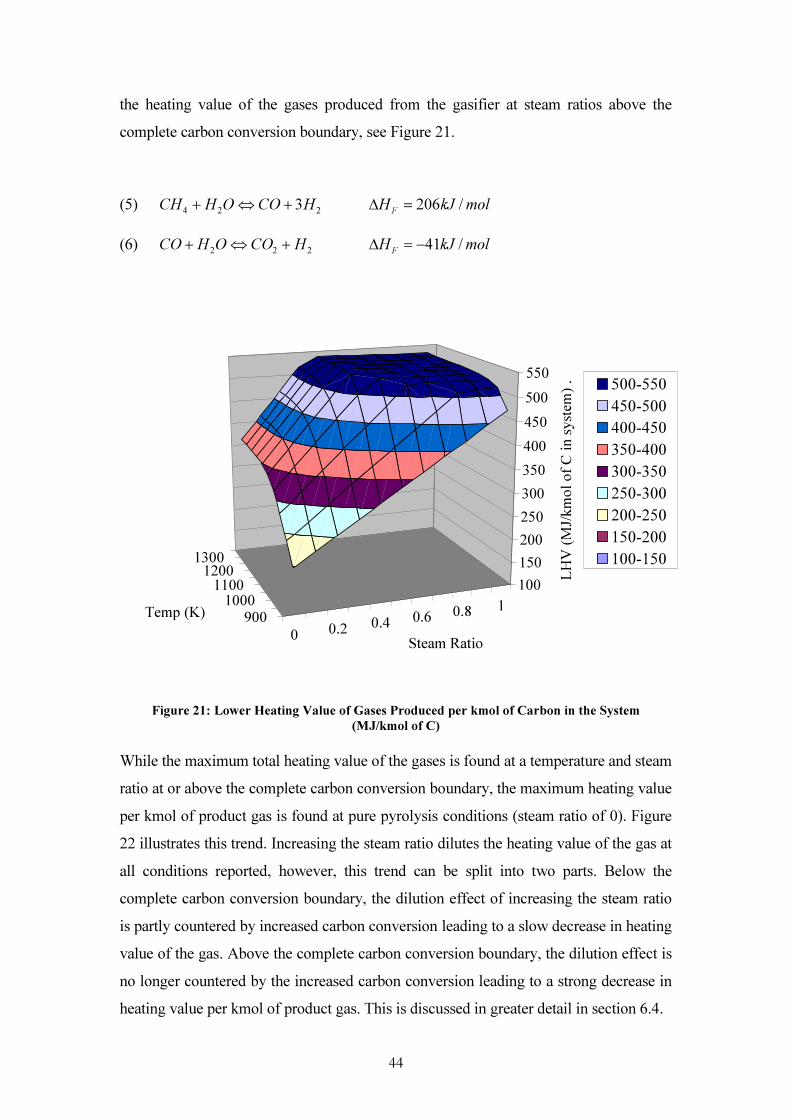
44

the heating value of the gases produced from the gasifier at steam ratios above the complete carbon conversion boundary, see Figure 21. (5) molkJHHCOOHCH F /2063 224 =∆+⇔+

(6) molkJHHCOOHCO F /41222 −=∆+⇔+

0 0.2 0.4 0.6 0.8 19001000

110012001300

100150200250300350400450500550

LHV

(MJ/k

mol o

f C in

syste

m) .

Steam RatioTemp (K)

500-550450-500400-450350-400300-350250-300200-250150-200100-150

Figure 21: Lower Heating Value of Gases Produced per kmol of Carbon in the System

(MJ/kmol of C) While the maximum total heating value of the gases is found at a temperature and steam ratio at or above the complete carbon conversion boundary, the maximum heating value per kmol of product gas is found at pure pyrolysis conditions (steam ratio of 0). Figure 22 illustrates this trend. Increasing the steam ratio dilutes the heating value of the gas at all conditions reported, however, this trend can be split into two parts. Below the complete carbon conversion boundary, the dilution effect of increasing the steam ratio is partly countered by increased carbon conversion leading to a slow decrease in heating value of the gas. Above the complete carbon conversion boundary, the dilution effect is no longer countered by the increased carbon conversion leading to a strong decrease in heating value per kmol of product gas. This is discussed in greater detail in section 6.4.

45

Figure 22: Lower Heating Value of Product Gas (MJ/kmol of gas)

These two figures give contrary advice on how to operate a gasifier. Figure 21 shows the total heating value of the product gas produced is maximised near the point of complete carbon conversion. Low steam ratios result in dramatic reductions in the total heating value, while large steam ratios do not significantly affect the total heating value. This suggests that to be confident of high total heating value, steam ratios should be high. However, Figure 22 shows that the molar heating value of product gas decreases sharply with increasing steam ratio beyond the complete carbon conversion boundary. The optimal operating point is, then, at the complete carbon conversion boundary balancing total heating values of gas and molar heating values. At this point it should be noted that gasifiers generally have a bed of char. This acts as a bank of stored char. Operating below the complete carbon conversion point will exhibit the trends shown in the above figures but will also increase the amount of char in the bed. Conversely, operating above the carbon conversion boundary will decrease the amount of char in the bed. However, the trends shown above will not be apparent until the all the char in the bed is gasified and no more solid carbon can enter the gas phase.

46

Therefore, there is a buffer period when operating above the complete carbon conversion layer before the strong dilution effect, shown in Figure 22, occurs. In updraft gasifiers the bed height can be monitored and the wood feed rate controlled so as to maintain a constant bed height. Maintaining a constant bed height will ensure that the gasifier is operating at the complete carbon conversion boundary. FICFB gasification, however, is more difficult to control so as to operate at the complete carbon conversion boundary because the char is in a fluid-bed. From an equilibrium point of view, operating beyond the complete carbon conversion boundary will result in insufficient char being carried to the CFB for combustion and it will be necessary to combust additional fuel to maintain temperature in the BFB. However, the reaction rates of char gasification have been proven to be slow (for instance Kersten, Prins et al. (2003) suggest that the residence times in atmospheric CFB biomass gasifiers at temperatures of 700-1000˚C are not sufficient for the char gasification reactions to proceed to a significant extent), therefore, char may be conveyed through the chute before it has the opportunity to gasify to the extent dictated by equilibrium. Hence, controlling the level of fluidization in the chute may remove carbon from the reaction system, therefore, leading to the complete carbon conversion boundary being seen at lower steam ratios than otherwise anticipated. A corollary effect of this is that the need for additional fuel in the CFB to maintain temperature in the BFB will be reduced. Operating below the complete carbon conversion boundary will result in excessive amounts of char in the system and will decrease the oxygen levels in the CFB. This could lead to excessive air rates in the CFB, in order to compensate for increased combustion, leading to increased temperature in the BFB. The control of steam rates (or wood feed) to maintain desired char levels is an area where further development of the CAPE FICFB system is required.

47

6.8 Effect of Char Circulation

As discussed, inside a FICFB gasifier a portion of the biomass entering the BFB reactor leaves the reactor as char through the chute to the CFB. This process can provide some or all of the heat of reaction for the gasification; however, it also removes some reactants from the reaction vessel. The effect of char circulation is shown in Figure 23. It is assumed that the char leaving the system is only carbon. In the figure, the moisture content of the wood is 10wt% and the steam ratio is kept constant at either 0.1 or 0.5 mol/mol. The figure also assumes that the char circulation rates presented can be achieved. This assumes that for all circulation rates, except those less than the complete carbon conversion line for a steam ratio of 0.1, the char is conveyed to the CFB before it can be gasified to the extent dictated by equilibrium. Hence, the equilibrium composition for these circulation rates is calculated assuming that the circulated carbon (char) does not take partake in reaction.

Steam Ratio = 0.1 Steam Ratio = 0.5 Figure 23: Effect of Removing Char from the Reaction System (T=800˚K)

48

The point of maximum chemical efficiency is where the gasifier is self-sufficient. This means that the gasifier can meet its energy balance solely through the combustion of char in the CFB and no additional fuel is required. Figure 23 shows that in order for the FICFB gasifier to be self-sufficient char circulation needs to be around 18% for the conditions shown. To achieve this, the reaction rate of char gasification needs to be sufficiently slow to allow the desired char circulation as, if the system proceeded to the equilibrium composition, all the carbon will be in the gas phase and no char would be available to circulate to the CFB. Figure 23 shows that chemical efficiency is maximized where the gasifier is self-sufficient. After this point, chemical efficiency drops rapidly as excessive amounts of char are removed from the reacting system. However, it needs to be noted that this is only true if any excess in char circulation beyond the level required for self-sufficiency results in char being removed from the gasification system. In reality, excessive char circulation will result in either increased combustion in the CFB, which will lead to an increase in temperature of the whole system, or , if the cyclone and siphon can effectively transport the char back to the BFB, in the carbon being returned to the reacting system. In this case increasing char circulation beyond the self-sufficient levels will lead to a higher temperature in the BFB and, if the cyclone and siphon are effectively transporting char back to the BFB, result in the efficiency and composition remaining relatively constant at the self sufficient level. There will be a slight decrease in chemical efficiency due to a product gas having a higher temperature; hence, a greater proportion of the energy of the system will be residing in the thermal energy of the gas rather than in the heating value of the gas. Figure 23 also shows that increased char circulation reduces the heating value of a volume of product gas, as equilibrium tends to favour production of hydrogen over carbon monoxide and the methane yield decreases.

49

6.9 Optimum Operating Point

The optimum operating point for a gasifier is a compromise between a number of conflicting variables. Reaction rate controlled issues like tar destruction and carbon conversion are improved with increasing temperature. However, the chemical efficiency decreases with increased temperature due to increased sensible heat of the gas. Figure 24 illustrates the effect of temperature and steam ratio on major operational concerns of a FICFB gasifier. In all cases char circulation is set to minimum self-sufficient levels. The feed is assumed to have 10wt% (daf) moisture content.

Figure 24: Efficiency of a Gasifier against Steam Ratio

Figure 24 shows that at higher temperatures both the equilibrium volumetric heating value of the gas and the chemical efficiency decreases. At the lowest temperature and steam ratio depicted in Figure 24 there is a sudden decrease in efficiency. This is due to the gasifier forming solid carbon in excess of that required for the gasifier to be self-sufficient. Figure 24 suggests that, from an equilibrium point of view, the optimum operation point of a gasifier is at the lowest temperature and steam ratio that still converts all carbon not required for combustion in the CFB into the gas phase. However, important operational concerns such as tar destruction and the degree to which carbon conversion reaches equilibrium levels are largely determined by reaction rates. Hence, the optimum operating point can be informed by, but not be predicted solely by, equilibrium modelling.

50

7 Gasification Modelling Validation

7.1 Introduction

The results presented previously represent the product gas compositions that would be evident if gasifiers operate under conditions conducive to chemical equilibrium. Many gasifiers, particularly small-scale FICFB gasifiers, may operate without sufficient residence time or mixing to achieve chemical equilibrium. In these cases, the results presented previously should be taken qualitatively. Knowledge of chemical equilibrium can still educate the operator on the effects of changing operating parameters as shown in the following comparison of equilibrium against results from the University of Vienna FICFB gasifier; however, kinetic factors need to be acknowledged as well. In this chapter chemical equilibrium is tested against the product gas composition of three different gasifiers; the 1.7 MWth Page Macrae up-draft gasifier, the 100 kWth CAPE FICFB gasifier and the 100 kWth Vienna University of Technology FICFB gasifier, and modifications to equilibrium are suggested to improve the performance of the gasification modelling.

7.2 CAPE FICFB Gasifier

The FICFB principles are described in section 3.2 and the detailed description of the CAPE gasifier can be found in Brown, Dobbs et al. (2006). Dry gas compositions were obtained by sampling using a gas chromatograph. The water content of the gas was obtained by drawing five litres of gas through a dry ice and acetone cooled condenser. The condenser was weighed prior to sampling and after sampling so that the weight of condensable material in five litres of product gas could be obtained. The condenser was then heated to 100˚C and then re-weighed. The difference before heating and after heating gave the water content of the gas. The remaining material was taken to be tar.

51

Table 7 shows that the CAPE FICFB gasifier produces a product gas with significantly higher concentrations of methane, ethene and ethane than is predicted by equilibrium. This suggests that the steam-methane reforming reaction does not proceed to equilibrium under these gasification conditions. The concentrations of hydrogen and carbon monoxide are lower and the concentrations of water vapour and carbon dioxide are higher than is predicted by equilibrium. It is difficult to infer from this how well the water-gas shift reaction tends to equilibrium as the presence of reasonable concentrations of hydrocarbons in the CAPE product gas means that carbon and hydrogen are bonded as methane, ethene or ethane rather than bonded in a form that can partake in the water-gas shift reaction.

Table 7: CAPE FICFB Gasifier Product Gas Composition (mol basis)

Conditions Steam Fluidizing Bed

Air Fluidizing Chute and Siphon

Steam Fluidizing Bed and Siphon

Air Fluidizing Chute Bed Temp (˚C) 700 730

CAPE Equilibrium CAPE Equilibrium CH4 8.4% 2.1% 9.0% 1.1% H2 14.2% 34.7% 16.4% 41.4% CO 20.6% 28.9% 21.1% 28.8% CO2 15.4% 11.0% 13.0% 10.0% N2 20.4% 17.2% 10.9% 8.8% H2O 19.2% 8.6% 26.0% 10.6% C2H4 2.2% 0.0% 2.5% 0.0% C2H6 0.5% 0.0% 0.5% 0.0%

Lower Heating Value (MJ/NM3wet) 8.2 7.9 9.1 8.2

Equilibrium Gas Yield to Measured Gas Yield

(kmol/kmol) 1.18 1.23

Ratio of Equilibrium to Actual Heating Value (With total gas yield taken into account)

1.14 1.11

52

Table 7 also shows that the CAPE product gas has a higher heating value on a volumetric basis than that predicted by equilibrium. However, the equilibrium composition results in a greater gas yield and, therefore, a greater heating value when the total volume of product gas is considered.

7.3 Vienna University of Technology FICFB Gasifier

The University of Vienna FICFB gasifier results are included to allow greater confidence in discussing the degree to which a FICFB gasifier conforms to the trends evident from chemical equilibrium modelling. University of Vienna results were used as results over a variety of operating conditions are not currently available from the CAPE gasifier. The results are taken from FICFB.at website (Rauch, 2006b). These results are for a pilot scale 100 kW FICFB gasifier. The details of which are described in Hofbauer, Veronik et al. (1997) and Fercher, Hofbauer et al. (1998). The major difference between Vienna’s gasifier and the CAPE gasifier are the positioning of the feed inlet and the positioning of the siphon circulating sand into the BFB. These results are based on a wood pellet feed and a natural catalytic bed material (assumed to be olivine). Figure 25 and Figure 26 present comparisons of the trends in product gas composition with temperature and steam ratio respectively. Both figures show that equilibrium over-predicts hydrogen and carbon monoxide and under-predicts carbon dioxide and methane. These results are very similar to that found from the CAPE gasifier. Indeed, the Vienna gasifier has a similar product gas composition to the CAPE gasifier when the additional nitrogen caused by fluidizing the CAPE gasifier’s siphon and chute with air is taken into account. Furthermore, both figures demonstrate that, while the equilibrium composition differs significantly from the small-scale FICFB product gas composition, the effect of varying temperature and steam ratio on the FICFB product gas composition is very similar to that predicted by equilibrium modelling.

53

Figure 25: Dry Product Gas Composition Trend with Temperature (Steam Ratio = 0.5kg/kg)

Figure 26: Dry Product Gas Composition Trends with Steam Ratio (T=875˚C)

7.4 Page Macrae Updraft Gasifier

The Page Macrae gasification has a stationary matrix of char inside the reactor and wood feed rates are controlled to maintain a stationary bed height. The product gas composition is, therefore, a result of predominantly char gasification reactions as the air (and steam) have to pass through between 800 mm to 1600 mm of char. A small amount of steam is added to the reactor to aid in the operation of the mechanical grate. Drying and devolatilisation of the wood feed will also contribute to the final composition but will not be the dominant mechanisms, as in FICFB gasification. It should be noted that the Page Macrae gasifier is considerably larger than both FICFB

54

gasifiers considered here by a factor of more than 10 (1 MWth+ against 100 kWth). Differences between how well equilibrium describes the product gas composition of the Page Macrae gasifier compared to the FICFB gasifiers are, then, caused by a combination of scale and gasification type. Results are obtained using the same methodology and equipment as used for the CAPE gasifier results. Figure 27 presents results from the 3rd of August 2006, where the bed height was raised from 850mm to 1250m and then from 1250mm to 1600 mm. During the day the bed temperature remained between 560˚C and 620˚C and primary air fluctuated between 4.2 and 7 kg/min.

0.0%

10.0%

20.0%

30.0%

40.0%

50.0%

60.0%

10.00 11.00 12.00 13.00 14.00 15.00 16.00 17.00Hours Since Midnight on 3rd of August

Dry G

as Co

mposi

tion (

molar

basis

)

NitrogenCarbon MonoxideHydrogenCarbon DioxideMethane

Bed Height = 850mm Bed Height = 1250mm Bed Height = 1600mm

Figure 27: Page Macrae Dry Gas Composition for 3rd of August, 2006

The constant product gas composition with varying bed heights is a good indicator that equilibirum has been reached. Greater bed heights will cause greater residence times and more gas-solid contacting. In a system that hasn’t reached equilibirum, this should move the compostion towards equilibirum. Furthermore, as primary air rates stay reasonably constant and feed rate is controlled to maintain the bed height at each set-point, the primary effect of increased bed height is that more carbon is available for gasification. Section 6 shows that for systems whose equilibrium is at or below the

55

complete carbon conversion boundary, the equilibirum composition is insensitive to additional carbon explaining the constant composition presented in Figure 27. A comparison of measured composition against that predicted by equilibrium modelling is presented below in Table 8. Table 8 uses the elemental abundances derived from the measured dry gas composition and with the water content of the gas adjusted so that equilibrium results in a stable char bed levels (minimum complete carbon conversion).

Table 8: Comparison of Page Macrae Results with Equilibrium Measured Equilibrium

Bed Temperature (˚C) 560 to 625 570 620 650 Dry Composition

Hydrogen (mol %) 13 to 19 21 20 19 Methane (mol %) 2 3 1 1

Carbon Monoxide (mol %) 19 to 22 9 16 21 Carbon Dioxide (mol %) 12 to 14 22 17 13

Nitrogen (mol %) 45 to 51 45 46 46 Lower Heating Value (MJ/Nm3) 4.1 to 5.1 4.1 4.4 4.6

Water Content (mol% wet basis) 30 to 50 20 12.75 8 * Ethane and Ethene are present in the Page Macrae product gas in levels less than 0.4% Table 8 shows that the Page Macrae gasifier operates close to equilibrium, as is expected due to the constant product gas composition with respect to bed height. Two discrepancies, however, are apparent. Firstly, equilibrium requires a temperature which is representative of the reacting system. Updraft gasification has a considerable temperature range throughout the char bed due to the combination of exothermic combustion and endothermic gasification reactions occurring. The temperatures, in Table 8, show the maximum measured temperature in the bed. However, bed temperature is measured at only four points and, therefore, the actual maximum temperature could be different to this. The gas composition is most consistent with an equilibrium temperature of 650˚C, which is 25˚C to 90˚C greater than the temperatures recorded but could easily be occurring in and around the combustion region. This suggests that the final gas composition is determined predominantly by the hotter regions of the char bed. Secondly, the measured water content differs greatly from that predicted by equilibrium. The most logical explanation of why the water content of the product gas may be greater than that predicted by equilibrium is that the fuel is screw-

56

fed on to the top of the bed. Therefore, the moisture released from drying of the fuel does not pass through the char bed and may not partake in reaction.

7.5 Improving Equilibrium

Equilibrium was proposed initially as a first-step in gasification modelling. For small-scale FICFB gasification it has proven to be a poor first step. However, until a greater sample of compositions is available (as of Sept, 2006, full datasets had been collected from only two gasification runs at CAPE and neither offer compositions representative of the desired operating conditions) it is not feasible to undertake detailed study into the adaptation of equilibrium. Page Macrae, on the other hand, are significantly further developed in their project and a significant dataset from their updraft gasifier was able to be collected (one week of data at desired operating conditions). Therefore, an improved equilibrium model for updraft gasification is proposed.

7.6 Modified Equilibrium for Updraft Gasification Modelling

Modelling of up-draft gasification can be improved by adapting equilibrium so that the approach is more representative of the mechanisms occurring in up-draft gasification. Analysis of the Page Macrae system and comparison with pure chemical equilibrium suggests that fuel drying occurs at low temperature on the top of the bed. Therefore, the fuel moisture has short residence times and little opportunity for solid-gas or gas-gas contacting. Modelling of the updraft gasification product gas compositions can be improved significantly by removing fuel drying from the equilibrium calculation. A schematic of this approach is shown below, in Figure 28.

57

Figure 28: Modified Equilibrium Schematic

The Page Macrae fuel has a moisture content of 30.3% (wet basis) (See Appendix A.12). This moisture content corresponds to 0.18 moles of fuel moisture entering the gasifier for every mol of wood (C0.32 H0.48 O0.20) feed. Balancing the carbon in the product gas with the carbon in the wood feed and allowing for the carbon removed with the ash (4% of carbon entering the gasifier), it can be shown that 1.14 moles of wood are required to produce 1 mol of dry product gas. This 1.14 moles of wood carries 0.21 moles of fuel moisture. Therefore, there is 0.21 moles of fuel moisture for every mol of dry product gas. Combine this with the equilibrium composition derived in section 7.4 and the resulting composition closely mirrors the measured composition, shown in Table 9.

Table 9: Modified Equilibrium Measured Modified

Equilibrium Bed Temperature 560-625 650 Hydrogen (mol%) 13 to 19 19 Methane (mol%) 2 1

Carbon Monoxide (mol%) 19 to 22 21 Carbon Dioxide (mol%) 12 to 14 13

Nitrogen (mol%) 45 to 51 46 Total Water Content (mol% wet basis) 30 to 50 28.9

Ratio of Fuel Moisture to Total Water in Product Gas 70.5% Ratio of Equilibrium Water to Total Water in Product Gas 29.5%

Equilibrium Composition Fuel Moisture

Wet Fuel

Product Gas

Dry Fuel Fuel Drying Gasification

Equilibrium

Ash & Char

58

7.7 Conclusions

Pure chemical equilibrium does not estimate the product gas composition of small-scale FICFB gasification well. The primary deficiency is the prediction of low methane yields and negligible higher hydrocarbons. Real small-scale FICFB gasifiers have methane mol fractions (dry basis) of 5-15% and non-negligible levels of ethane and ethene. In terms of the model, this means that FICFB gasifiers exhibit a tendency for the steam methane reforming reaction to be shifted towards greater methane formation. From a heating value perspective, this is of concern as the steam methane reforming reaction is strongly endothermic reaction and equilibrium will, therefore, result in over-prediction of heating value. In contrast, the water gas shift is not strongly exothermic and therefore has less influence on the heating value of the gas. (5) molkJHHCOOHCH F /2063 224 =∆+⇔+

(6) molkJHHCOOHCO F /41222 −=∆+⇔+

Equilibrium over-predicts hydrogen and carbon monoxide mol fractions and under-predicts carbon dioxide and methane mol fractions. Incomplete breakdown of the hydrocarbons in FICFB gasification results in less hydrogen being available to undergo the water-gas shift reaction and causes equilibrium to over-predict the amount hydrogen and carbon monoxide and under-predict the amount of carbon dioxide. However, equilibrium does perform well at predicting the effect of changing the temperature of gasification and the steam ratio as shown by Figure 25 and Figure 26 . This indicates that the trends described by chemical equilibrium modelling are relevant to all gasifiers, even though the predicted compositions may not be accurate. Updraft gasification, with the stationary char matrix, produces a gas whose composition is predicted well by a modified equilibrium. It is, therefore, reasonable to suggest the trends discussed in section 6 are applicable to updraft gasification. Equilibrium, then, is a valuable tool in educating decisions about updraft gasification especially when assessing modifications to operational procedures and during the design phase.

59

8 Economic Modelling Method

8.1 Process Description

This thesis presents economic models of four energy processes in order to provide information for the discussion of the optimal design, optimal scale and economic feasibility of integrating gasification into New Zealand’s wood industry. The four processes considered are gasifier-gas turbine combined cycle, gasifier-gas turbine, gasifier-gas engine and gasifier-boiler. The gas turbine combined cycle and gas engine processes were chosen as they were identified as the most appealing electricity generation options for gasification by Li and Pang’s (2005) review of gasification technology. The boiler option is investigated as it represents a non-cogeneration low capital option. The following section presents a literature review of the current state of technology of the components making up these processes and a rationale of the modelling methodology. The four processes share a number of similar components but differ in key areas such as gas cleaning and product gas combustion. The shared components of the four processes will be discussed first and then the components specific to a particular process.

8.1.1 Biomass Drying

Biomass drying requirements are determined by the moisture content of the fuels used for gasification. An MDF plant has access to a number of internal wood waste streams as well as a variety of imported fuels. Information from Li and Pang (2006) and BIGAS consortium objective three suggests that the internal waste streams have moisture contents ranging from 10% to 180% (OD basis) and the imported wood streams have a moisture content ranging from 40% to 60% (OD basis). Typical FICFB gasification operates with a feed moisture content of 25% (OD basis) (Schuster, Loffler, Weigl, & Hofbauer, 2001) hence, some drying of the biomass is required. Brammer and Bridgewater (1999) present a review of drying technologies for gasification which identifies direct rotary cascade driers, which use combustion products as the drying medium, as the conventional lowest risk option. They also discuss the merits of using steam for indirect rotary drying and pressurized fluid-bed drying. The merit of indirect rotary drying is that low-grade waste heat from cooling a gas engine can be used; however, indirect drying is more capital intensive than direct drying. Fluid-bed systems

60

have merit as, although they generally have to be specifically designed resulting in high capital costs, they have very low emissions and have good scale up characteristics. Therefore, they may be an appealing option for large-scale plants. A rotary cascade drier is the option used in the modelling as it represents the most widely used industrial drier (Brammer & Bridgwater, 1999) and costing information is available for it (Brammer & Bridgwater, 2002). This drier is shown in Figure 29. It should be noted that for a large-scale gas engine plant, where there is a large amount of waste heat from cooling the engine, it may be more economical to use a band dryer heated with warm air from the engine coolant system.

Figure 29: Rotary Cascade Drier (Brammer & Bridgwater, 1999)

8.1.2 Feed Handling and Storage

Biomass covers a group of substances with widely varying physical properties. Feed handling and storage options will vary considerably depending on the composition and flow properties of the biomass being handled. The advice of Brightwater Engineering (R Lines, pers. Comm.) was sought for developing a costing relationship for feed handling and storage. Three scenarios were costed: a small plant (2-6 MWth), a medium plant (6-20 MWth) and a large plant (greater than 20 MWth). Details of these can be found in Appendix B.1.

61

8.1.3 Gasification

The gasifier is the most novel item in the process and there is no database of actual gasifier cost histories available for reference. Published cost correlations for gasifiers (Caputo, Palumbo, Pelagagge, & Scacchia, 2005; DSIR, 1982; A. P. C. Faaij, Meulemann, & Van Ree, 1998; Rodrigues, Faaij, & Walter, 2003) vary greatly. The most concerning difference in published cost correlations is the variation in scaling factors applied. Generally costs can be estimated from a known cost and scale using the formula below:

Cost2 = Cost1 (Size2/Size1) Scale Factor

Literature reported scale factors for fluid bed gasifiers vary from 0.917 (Caputo, Palumbo, Pelagagge, & Scacchia, 2005) to 0.485 (DSIR, 1982). The inconsistency in scale factors leads to a wide variation in the cost estimates, with the costs estimates by Caputo, Palumbo et al. (2005) for a 30MWth fluid bed gasifier being four times that of an equivalent sized gasifier costed using Faaij, Meulemann et al.’s (1998) correlation, and 25 times that of a gasifier costed using the DSIR’s (1982) correlation. Due to this inconsistency, a bottom up approach to costing has been taken. This approach builds the cost of a gasifier up from its individual parts and applies relevant installation factors to estimate the installed cost of the gasifier. The FICFB gasifier is essentially made up of four process vessels, a cyclone, two gas burners and a blower. The four process vessels represent the bubbling bed reactor, the circulating bed reactor, the chute and the siphon. Each process vessel is lined with 100mm of hot-face refractory and a further 150mm of cold-face refractory. The geometries of the vessels are assumed to be circular and calculated assuming similar superficial gas velocities as the lab scale gasifier. These are given in Table 10.

Table 10: Design Velocities for FICFB gasifier CFB Gas velocity 7 m/s BFB Gas Velocity 1.5 m/s Chute Velocity 0.15 m/s Siphon Velocity 0.15 m/s

According to Ulrich (2005), fluidized beds typically have a bed height-to-diameter ratio of two and a freeboard height-to-diameter ratio of 0.4. Therefore, the height of the bubbling fluid bed reactor is assumed to be 2.4 times the diameter. This varies considerably from the 100 kWth gasifier at CAPE, but should be representative of the

62

height-to-diameter ratio of commercial scale plants. The circulating bed reactor is assumed to be two meters longer than the bubbling bed to allow for the chute, siphon and cyclones. The chute is modelled as having a height three times its diameter and the siphon has a height two times its diameter. Costing for these individual components are estimated by correlations from Bouman, Jesen et al. (2004) and Ulrich and Vasudevan (2005) and by approaching suppliers for burners (Aquaheat, pers. comm.) and refractory (Thermal Ceramics, pers. comm.). The relationships are shown in Table 11

Table 11: Gasifier Cost Breakdown Component Cost Relationship LPG Burners 12000 [Nburners][0.1*LHVbiomass(MW)]0.7

Blowers 771[Qair (m3/s)]*+2400 Steel Casing (3952*[Dr(m)]+965)*[Hr(m)](0.9749-0.0518[Dr(m)])

Cyclones 2,330[Qcylone (m3/s)].912 Refractory

Lining 48/25*[Mhotface(kg)]+28/15*[Mcoldface(kg)] Nburners is the number of gas burners required LHVbiomass is the thermal energy input into the gasifier Qair is the volumetric flow of the air through the CFB Dr is the diameter of the reactor Hr is the height of the reactor Mhotface is the mass of hot-face refractory required Mcoldface is the mass of cold-face refractory required Qcyclone is the volumetric flow through the cyclone increased by the volume of refractory lining A factor approach is used to account for civil, electrical, piping, instrumentation and contingency costs. The factors used are shown in Table 12. Due to the novel nature of the FICFB technology there is considerable uncertainty in this estimate.

Table 12: Installation Factors for the Gasifier (Ulrich & Vasudevan, 2005) Equipment (delivered) 1 Equipment, Installation 0.43 Piping 0.39 Structural foundations - Electrical 0.17 Instruments 0.13 Battery-limits building and service 0.35 Excavation and site preparation 0.22 Auxiliaries 0.55 Total physical plant 3.24 Field expense 0.43 Engineering 0.43 Direct plant costs 4.1 Contractor's fees, overhead, profit 0.17 Fixed-capital investment 4.27 Contingency 2.135 Total fixed-capital investment 6.405

*These are typical installation factors as suggested in Ulrich and Vasudevan (2005). The contingency however has been increased to reflect the novel nature of the technology. The contingency factor is within suggested ranges from Ulrich and

Vasudevan (2005) for novel processes and was chosen so that the gasifier costs are similar to those reported in the literature, see (DSIR, 1982; A. Faaij et al., 1997; Rodrigues, Faaij, & Walter, 2003)

63

8.1.4 Gas Cleaning

The BIGAS Consortium has not yet undertaken investigation into gas cleanup measures. Hence, the gas cleaning for the model is based on the Gussing process (Hofbauer, Rauch, Bosch, Loch, & Aichernig, 2002) and recommendations by Scharpf and Carrington (2005). Prior to gas cleaning, the gas is cooled with heat recovery to 170°C. The first stage of the gas cleaning is a fabric filter used to remove particles and some tars. The second stage is a bio-diesel scrubber, which is used to remove the remaining tars and any condensate. Rauch (2006a) reports this gas cleaning scheme uses 15 kg/hr of precoat material for the bag filters (activated carbon and hydrated lime have been tried) and 15 l/hr of bio-diesel for a 8 MWth plant. The gas leaves the scrubber at 40°C and can be fed directly into a gas engine or fuel compressor of a gas turbine. This cleaning regime has been proven to be sufficient for gas engines, with Gussing having nearly 10,000 hours of operation (Herdin, Robitschko, Klausner, & Wagner, 2003). However, it remains to be seen whether this arrangement will clean the gas sufficiently for gas turbines. Table 13 shows the gas qualities required for different prime movers. Table 13: Required Gas Quality for Gas Engines and Turbines (Scharpf & Carrington, 2005) Guascor Engines Jenbacher Engines Gas Turbines Particles >5microns 0 mg/Nm3 Not Specified 10ppm Particles <5microns 108 mg/Nm3 Not Specified Tars 108 mg/Nm3 5 mg/Nm3 5mg to 5g/ Nm 3

Sulphur 2520 mg/Nm3 700 mg/ Nm 3 1 to 7000 ppm Ammonia 54 mg/Nm3 50 mg/ Nm 3 50 ppm Chlorine 126 mg/Nm3 100 mg/ Nm 3 0.5 ppm Silicon 7.2 mg/Nm3 200 ppm Not Specified Units have been converted on the basis of 1Nm3 of natural gas having 10 kWh or 36 MJ of energy content.

64

8.1.5 Gas Turbine

Operating conditions for the gas turbine have largely been based on values for gas turbines available on the market today as reported by the Gas Turbine World Handbook (2005) which lists specifications for 132 turbines, and Traverso, Cazzola et al. (2004) who give greater detail on 20 turbines. These values are given in Table 14.

Table 14: Gas Turbine Operating Parameters (Traverso, Cazzola, & Lagorio, 2004)

Average Maximum Temperature 1175˚C Average Exhaust Temperature 510˚C Average Pressure Ratio 16.5

The maximum temperature and pressure ratio, shown in Table 14, has been used in the model. Efficiencies and costs are based on fitting a line to data from the Gas Turbine World Handbook (2005). The fitted line for costs is shown in Figure 30. These costs are for a skid-mounted single fuel gas turbine, electric generator, air intake with basic filter and silencer, exhaust stack, basic starter and controls and conventional combustion system.

-

5,000,000

10,000,000

15,000,000

20,000,000

25,000,000

30,000,000

35,000,000

40,000,000

45,000,000

0 5 10 15 20 25 30 35 40 45 50Base Load Rating (MWe)

Purch

ase Co

st (NZ

$200

5)

0%

5%

10%

15%

20%

25%

30%

35%

40%

45%

50%

LHV

Effici

ency

LHV Efficiency

Purchase Cost

Figure 30: Capital Cost and Efficiency of Gas Turbines (Gas Turbine World, 2005) The combustion chamber of a gas turbine may require modification to be suitable for burning lower calorific value fuel. The fuel nozzle of a standard gas turbine is designed for natural gas, which has an HHV of around 39 MJ/Nm3 (Baines, 1993). Substantially

65

larger flows through the fuel nozzle will be required to achieve similar levels of thermal energy when a low heating value fuel is used. FICFB product gas has a heating value around 10-11 MJ/Nm3 and therefore, for similar thermal input, four times more fuel will be required to flow through the fuel nozzle compared to the natural gas design volume flow. This larger flow can lead to significant pressure drop across the fuel nozzle. Therefore, replacement of the fuel nozzle may be required. The entire combustion chamber may require modification or replacement if a significantly lower heating value fuel is used. Due again to the larger volumes, the combustion chamber may need to be expanded and modified to better suit the lower heating value gas. Rodriques et al. (2003) reports estimates on the costs of these modifications based data provided by a GE gas turbine supplier. The modifications are split into three categories and are shown in Table 15.

Table 15: Modifications Required to Gas Turbine Modification Cost (% of GT capital cost) Burner Modification 2% Burner Replacement 5% Combustion Chamber Replacement 20%

For modelling purposes, it has been assumed that gas turbine purchase costs are increased by 20%. However, due to FICFB gasification producing a moderate (10-11 MJ/Nm3), rather than low (5-7 MJ/Nm3), calorific value fuel with a high hydrogen content, it may be that the required modifications are reduced. FICFB produces a gas with a composition similar to IGCC from refinery coke. GE has gained 340,000 hours experience in operating IGCC turbines and has developed combustion chamber designs specifically for fuels from gasification (R. Jones & Shilling, 2003). There are currently more than 20 IGCC plants operating, showing that the technology for combined cycle power generation from gasification is developed. Figure 31 shows a selection of the LHV’s of the producer gas used in these combined cycles, as well as the heating value of the producer gas from Gussing, a biomass FICFB gasifier. The chart demonstrates that the producer gas from biomass FICFB gasification is similar or of higher quality than many IGCC producer gases and, therefore, should be able to be fired in turbines adjusted for IGCC use. The major difference between IGCC applications and biomass FICFB gasification applications is not in the composition of the producer gas but the scale of power generation. The IGCC applications range from 40MWel to 800MWel,

66

while 40MWel would represent a large biomass application due to transportation costs of biomass.

-

50,000

100,000

150,000

200,000

250,000

300,000

Sierra

Pacif

icTo

nghu

aSa

rlux

ILVA PS

IPe

rnis

Exxo

nSing

apore

El Do

raro

Motiv

aDela

ware

Tamp

aPIE

MSA

Gussi

ngSc

hwarz

ePum

pe Fife

LHV

(kJ/km

ol)

Figure 31: IGCC Producer Gas Heating Values

8.1.6 Steam Cycle

Steam cycles can have a variety of operating conditions. High temperatures and pressures allow for more efficient cycles but high temperatures and pressures incur greater capital and operating costs. Therefore, there is an optimal economic operating condition for steam cycles. In a New Zealand manufacturing environment this has been assumed to be equal to the values given in Table 16. These values were reported for new cogeneration plant by Energy for Industry (2005), whose core business is on-site industrial scale energy plants in New Zealand.

Table 16: Steam Cycle Operating Parameters (Energy for Industry, 2005) Maximum Steam Temperature 450°C Maximum Steam Pressure 60 bar

It has been assumed that a pass-out turbine is used so that process steam can be extracted at nine bar. To evaluate the conditions at the turbine exhaust, it is assumed that a 10°C approach temperature across the condenser can be reached and that cooling

67

water can extract the heat at 30°C rising to 40°C. This gives a minimum steam cycle temperature of 50°C and dictates the minimum pressure given an assumption of steam turbine efficiency. It is assumed that steam turbines have an adiabatic efficiencies of 75%, which is mid-range of those referenced in Smith Van Ness et al. (1996). Process steam is generated at nine bar in all scenarios. Four bar steam is attained by reducing the pressure in the nine bar steam through use of an expansion valve and then saturating the steam.

8.1.7 Gas Engine

Gas engines are an appealing prime mover for smaller scale power generation. The requisites for gas cleanup are reduced and are better known. There is also greater operational experience of gas engines on producer gas than there is for gas turbines. On scales smaller than around five MWel they are a more efficient electrical generation option than gas turbines. Jenbacher engines have been used for this modelling, due to their experience in operating on exotic gases, particularly thousands of operating hours at the Gussing plant which operates a FICFB gasifier. Jenbacher engines represent the more efficient, reliable and costly end of the gas engine market. It is possible to buy cheaper engines which will run on producer gas. The cheapest capital option is to convert a diesel engine to spark ignition. This could be an appealing option for sites where capital cost is limited and reliability is not essential. However, for the wood industry, supply of process heat is essential to their manufacturing and reliability is paramount. A typical industrial cogeneration scale gas engine is a turbocharged, inter-cooled, spark ignition engine. They can either be operated at stoichiometric air for maximum power or at lean-burn conditions which minimize NOx emissions. For modelling purposes, it is assumed that the engine is operated in lean-burn conditions, with an air to fuel ratio of 1.6 times the stoichiometric air-fuel ratio (Major, 1995). For cogeneration the engines are equipped with a generator connected directly to the engine drive. Heat is recovered from the cooling water and oil circuits as well as the exhaust gases. Water-to-water and

68

water-to-oil exchangers are used to recover heat from the cooling water and oil circuits. The exchangers cannot be connected directly to the process heat medium due to problems with corrosion, pressure and thermal shock (Major, 1995). Table 17 shows an energy balance for a gas-engine based on data from Jenbacher (G Herdin, pers. comm.). Steam generation from the exhaust gas is typically greater than that shown in Table 17; however, to ensure an exhaust temperature of 380°C required for MDF process heat, some steam generation is sacrificed. The engine cooling and heat loss are assumed to be constant relative to the thermal energy input. Therefore, increased electrical efficiency is assumed to be at the expense of steam generation from the exhaust gas.

Table 17: Energy Balance for a Jenbacher JMS 620 Engine (G Herdin, pers. comm.). Energy Form Heat Source Engine Efficiency

(based on LHV of Product Gas)

Power

Less than 3.8MWth 1.456[LHVProduct Gas (MW)]+37.3%

Greater than 3.8MWth 42.9%

Steam (175.5°C) Exhaust Gas Less than 3.8MWth

5.5 to 11.1% Greater than 3.8MWth

5.5% Hot Water (110°C) Charge Cooling 8.5% Hot Water (110°C) Cooling Water 9.4% Hot Water (110°C) Oil Cooling 5.0%

Heat Loss Engine 8.7% Exhaust Gas Exhaust Gas 20%

A major consequence of using a gas engine rather than a gas turbine is a proliferation of low grade heat. Gas engines produce a large proportion (23-30%) of low grade heat, typically high temperature hot water. An MDF plant has minimal need for high temperature hot water and may require cooling towers to dispose of this heat.

The costs for gas engines are based on costs from GE Jenbacher and are presented in Table 18. The costs shown are purchase costs for the gas engine, acoustic enclosure, heat exchangers, coolers and piping.

69

Table 18: GE Jenbacher Gas Engine Costs and Power Outputs (G Herdin, pers. comm.)

Model Power Output (kW)

Purchase Cost (€)

JMS 208 208 285,000 JMS 312 365 330,000 JMS 316 487 440,000 JMS 320 608 550,000 JMS 612 1216 695,000

An important point to note is that the power outputs stated in Table 18 are for engines running on natural gas. In general, burning fuels of lower calorific value in engines of the similar cylinder capacity and engine speed results in lower thermal input into the engine and, hence, lower power output. Brammer and Bridgwater (2002) and Wereko-Brobby and Hagan (1996) estimate the de-rating of an engine on non-standard fuel by assuming constant electrical efficiency and constant volumetric flow-rate of air-fuel mixture into the engine. Hence, power output of an engine is directly proportional to the heating value of the given volume of the air-fuel mixture. LHV of Producer Gas & Air Mix (MJ/m3) = Output of Engine on Producer Gas (MWel) LHV of Natural Gas & Air Mix (MJ/m3) Output of Engine on Natural Gas (MWel)

The calculation for this equation is given in Appendix B.2. This generally results in significant de-rating of the engine and a compensating increase in capital cost to attain a similar power output engine when running on the low heating value product gases. Rabou and Jansen (2001) give an increase in specific capital cost of 50% due to de-rating of the engine. However, FICFB product gas compositions require less air than natural gas to combust. Therefore, although their heating value is lower on a per mole of product gas basis, on a per mole of air-fuel mixture basis the heating value is comparable if not greater than natural gas. The concern with FICFB product gas is not the lower heating value but rather the high hydrogen content. The assumption of constant electrical efficiency on different fuels is only valid if similar compression ratios can be attained without knocking. Electrical efficiencies of engines are proportional to the compression ratio up to the point at which knocking occurs

70

(Wereko-Brobby & Hagan, 1996). High hydrogen fuels are less knock resistant and, therefore, unable to have large compression ratios. The degree to which the hydrogen affects the efficiency and cost of the engine is an important aspect for further study. For modelling purposes, no de-rating of the engine has been assumed, although it is expected that some additional costs will be incurred as the engine will have to be more knock-resistant than the standard engine.

8.1.8 Boiler

The gas boiler has been based on costing relationships presented in Ulrich and Vasudevan (2005) for a natural gas boiler.

8.2 Process Flow sheets

Process flow-sheets for the four processes are shown in the Figures 32-35. After the process flow-sheets an overview of the modelling method is presented followed by a discussion of the pertinent economic factors affecting cogeneration plant in New Zealand.

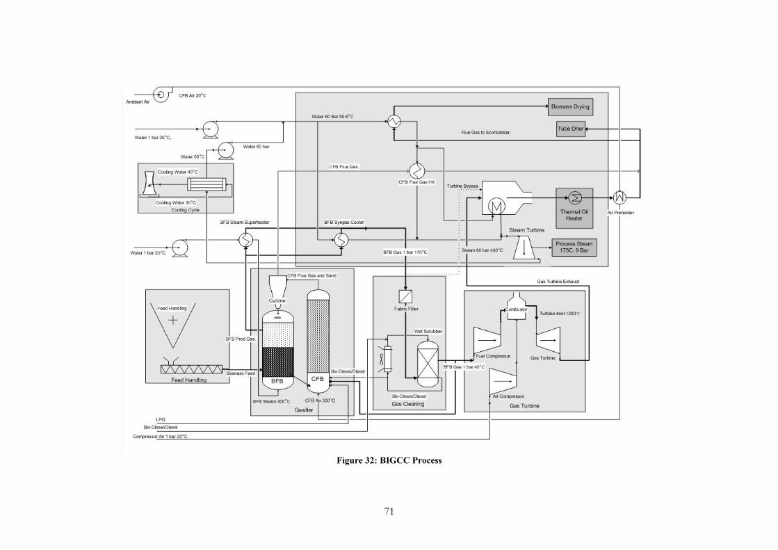
71

Figure 32: BIGCC Process

72

Figure 33: Gasifier-Gas Turbine Process

73

Figure 34: Gasifier-Gas Engine Process

74

Figure 35: Gasifier-Gas Boiler System

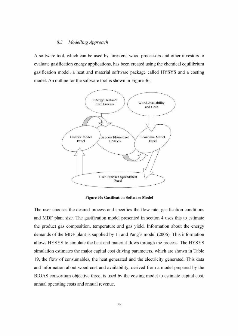
75

8.3 Modelling Approach

A software tool, which can be used by foresters, wood processors and other investors to evaluate gasification energy applications, has been created using the chemical equilibrium gasification model, a heat and material software package called HYSYS and a costing model. An outline for the software tool is shown in Figure 36.

Figure 36: Gasification Software Model

The user chooses the desired process and specifies the flow rate, gasification conditions and MDF plant size. The gasification model presented in section 4 uses this to estimate the product gas composition, temperature and gas yield. Information about the energy demands of the MDF plant is supplied by Li and Pang’s model (2006). This information allows HYSYS to simulate the heat and material flows through the process. The HYSYS simulation estimates the major capital cost driving parameters, which are shown in Table 19, the flow of consumables, the heat generated and the electricity generated. This data and information about wood cost and availability, derived from a model prepared by the BIGAS consortium objective three, is used by the costing model to estimate capital cost, annual operating costs and annual revenue.

76

Table 19: Capital Cost Parameters Major Plant Item Costing parameter Unit Feed Handling Volumetric flow of feed m3/s Gasifier – burners Heat release rate MW Gasifier – blowers Volumetric flow of air m3/s

Gasifier – steel Diameter and height of reactor m Gasifier – refractory Mass of refractory required kg Gasifier – cyclone Volume flow through cyclone m3/s Gas Bag Filter Volumetric flow of gas m3/s Venturi Scrubbers Volumetric flow of gas m3/s Gas Engine Electrical Output of Engine kWel Gas Turbine Electrical Output of Turbine kWel Steam Turbine Electrical Output of Turbine kWel Pumps Volumetric flow through pump m3/s Shell and Tube HX Area of heat exchanger * m2

Gas-fired Boiler Heat transfer required from boiler kWth Air to Air HX Area of heat exchanger m2

Steam Drum Diameter of steam drum m Flare Lower heating value of gas MWth Stack Diameter of stack m

* For heat transfer coefficients see Appendix A.11 Capital costs are estimated using costing relationships available in the literature (Bouman, Jesen, & Wake, 2004; Gas Turbine World, 2005; Ulrich & Vasudevan, 2005) and, where unavailable, through approaching suppliers (Aquaheat, pers. comm.; G Herdin, pers. comm.; R Lines, pers. comm.; Thermal Ceramics, pers. comm.). The costing relationships, shown in Table 20, give what Gerrard (2000) defines as a ‘study estimate’ which has a probable range of accuracy of ±20% to ±30%. While the level of accuracy is not high, modelling of this type allows estimation of the economic feasibility without detailed engineering, giving interested parties information on the general appeal and major factors influencing the economics of the project without significant capital outlay. Furthermore, a number of processes (this thesis looks at four) can be investigated and compared. The value in such modelling is that it allows decisions on whether a project has sufficient appeal to be continued, identifies the key areas for economic feasibility, and identifies the processes which are deserving of more detailed analysis. For further details about the costing model, refer to Appendix B.4.

77

Table 20: Capital Cost Estimating Relationships Major Plant Item Purchase Cost ($NZ) Bare Module Factor

(BMF) Installed Cost ($NZ) Source

Biomass Drying 15,739[13,333Qmoist(kW)(0.971/X2-0.479/X+11)+93.2]0.863 (Brammer & Bridgwater, 2002)

Feed Handling 448,300[Qfeed(m3/s)]0.577 (R Lines, pers. comm.) Gasifier 33,596 [LHVbiomass(MW)] + 487949

Gas Bag Filter 26,066 [QBFB(m3s]0.7055 4 Purchase Cost * BMF Pg 394 (Ulrich & Vasudevan, 2005) Venturi Scrubbers 24,446[QBFB(m3/s)]0.6832 6.3 Purchase Cost * BMF Pg 394 (Ulrich & Vasudevan, 2005)

Gas Engine

PGE(kWe) <330 2,446*[PGE(kWe]

330< PGE(kWe) <1400 1,614*[PGE(kWe] PGE(kWel) >1400 1,018*[PGE(kWel]

2.0 Purchase Cost * BMF (G Herdin, pers. comm.)

Gas Turbine 7,281*FPG*[PGT(kWel)]0.7284 3.5 Purchase Cost * BMF (Gas Turbine World, 2005) Steam Turbine 8,522[PST(kWel)]0.4524 3.5 Purchase Cost * BMF Pg 375 (Ulrich & Vasudevan, 2005)

Pumps 127*[Qpump(m3/hr)]+1720 3.5 Purchase Cost * BMF (Bouman, Jesen, & Wake, 2004) BIGCC HRSG 11678 MHRSG (kg/hr)0.81

(Caputo, Palumbo, Pelagagge, &

Scacchia, 2005) Shell and Tube HX 1,540[AHX(m2)]0.566 1.2775(Fm*Fp) +2.179 Purchase Cost * BMF (Bouman, Jesen, & Wake, 2004) Gas-fired Boiler 532*[QHX(kW)]0.805 3.12 Purchase Cost * BMF Pg 377 (Ulrich & Vasudevan, 2005) Air to Air HX 4,675[AHX(m2)]0.3992 1.2775(Fm*Fp)+2.179 Purchase Cost * BMF Pg 385 (Ulrich & Vasudevan, 2005) Steam Drum P1SD[DSD(m2)]P2SD 0.6995(Fm*Fp)-0.6086 Purchase Cost * BMF Pg 387 (Ulrich & Vasudevan, 2005)

Flare 2,599[LHVgas(MJ/s)]0.8709 1 Purchase Cost * BMF Pg 370(Ulrich & Vasudevan, 2005) Stack 41,867[Dstack(m)]2.0369 1.3 Purchase Cost * BMF Pg 366(Ulrich & Vasudevan, 2005)

*Simplified relationship. For complete costing information see Table 11 and Appendix B.4 Qmoist is the heat transferred to the biomass (kW) X is the mean biomass moisture content (%OD) Qfeed is the volumetric flow rate of feed into gasifier LHVbiomass is the thermal energy input into the gasifier QBFB is the volumetric flow rate of the producer gas PGE is the power output of the gas engine FPG is cost factor of modifying the gas turbine to producer gas (1.2 PGT is the power output of the gas turbine PST is the power output of the steam turbine Qpump is the volumetric flow through the pump MHRSG is the mass flow rate of steam through the HRSG AHX is the area of the heat exchanger Fm is the construction material factor and Fp is the pressure QHX is the heat transfer required from the boiler P1SD and P2SD are factors based on the pressure of the steam DSD is the diameter of the steam drum, which is derived by either the distance required for separation or the minimum liquid hold-up. LHVgas in the lower heating value of combustible gases Dstack is the diameter of the stack

78

8.4 HYSYS Simulation

The design philosophy for the processes was to ensure that each process met the heat demands of an MDF plant (both the 15.1 MW of process, see section 9.2, heat plus the heat required to dry the wood feed). This sets the scale of the gasifier-boiler plant, as it is a heat only plant, and sets the minimum scale for the gasifier-gas engine and gasifier-gas turbine combined cycle plants. Larger scales allow greater electricity production but will result in waste heat being generated. Table 21 shows a summary of the major process parameters

Table 21: Process Parameters Gasifier Heat-loss 5% of HHV of fuel in (Schuster, Loffler, Weigl,

& Hofbauer, 2001) Scrubber Inlet Temp 170°C (Hofbauer, Rauch, Bosch,

Loch, & Aichernig, 2002) Scrubber Outlet Temp 40°C (Hofbauer, Rauch, Bosch,

Loch, & Aichernig, 2002) Gas Engine Efficiencies (%)

Less than 3.8 MWel 1.46 MW(LHV Gas)+37.3% Jenbacher (2004a-d) Greater than 3.8MWel 42.9% (Jenbacher, 2004d)

Gas Turbine Efficiencies (%) 0.3 MW(LHV Gas)+28.0% (Gas Turbine World, 2005) Turbine Pressure Ratio 16.6 (Massardo & Scialo, 2000)

Turbine Inlet Temperature (°C) 1200°C (Massardo & Scialo, 2000)

Steam Turbine Inlet Temperature (°C) 450°C (Energy for Industry,

2005) Steam Cycle Maximum

Pressure (bar) 60 bar (Energy for Industry, 2005)

The economic appeal of each process is considered by calculating the net present value of each process over the range of valid scales. The net present values (NPV) are calculated as shown below:

on)DepreciatiprofitTax After (AnnualFactor Annuity Cost CapitalNPV ++−=

Where the Annuity Factor = ( )1 1

1 )tr r r

− + = ( )30

1 10.1 0.1 1 0.1) − +

= 9.43

The capital cost is assumed to occur immediately and the annual after-tax profit is assumed to occur each year for a lifespan of 30 years. A lifespan (t) of 30 years was chosen as this is the typical lifespan of a power plant according to Marsden, Poskitt et

79

al. (2004). This assumes a constant annual after-tax profit for each year and straight-line depreciation. This yields a simple calculation of NPV. However, if desired, the model provides sufficient information for analysis on the effect of varying electricity price, wood cost or cost of other supplies over time. The analysis presented here assumes a project life (t) of 30 years and a cost of capital (r) of 10%. Breakeven electricity price, the electricity price where the NPV of the project equals zero, is also calculated to give an idea of the sensitivity of the project to changes in electricity price. This can be used to educate discussion of the subsidies or the increase in electricity price that will be required to encourage investment in gasification energy plant that is currently uneconomic.

80

9 Economic Environment

9.1 Introduction

This thesis has, so far, introduced a model for predicting gasification product gas composition, discussed the components that make up a gasification energy plant and presented a model for predicting the economic appeal of gasification energy plant. Before the results of the economic feasibility of gasification energy plant are discussed, the economic environment that gasification energy plant have to compete in will be introduced. The Canterbury region is looked at specifically, as modelling data for the costs and availability of biomass for the Canterbury region are available. The costs and availability of biomass will vary throughout the country but, if care is taken, the discussion here should be generally applicable to New Zealand as a whole.

9.2 MDF Plant Energy Demand

A typical MDF line produces 120,000 m3 of MDF annually. Li (2005) gives the energy demands for a typical MDF site, shown in Table 22. A typical MDF plant has an overall load factor of 90% (Maloney, 1993). All processes discussed are designed to meet the heat demands listed in Table 22. Excess heat is used for feed drying or otherwise discarded through appropriate cooling. For presentation of the results from the economic modelling, process heat is assumed to be valued at $8/GJ (2.88 c/kWh) (East Harbour Management Services, 2005), however, the model allows for heat to be valued at any value the user specifies. A price of $8/GJ provides each process with minimum annual revenue of $3.4M. This revenue can be thought of as a payment from the MDF plant to the energy plant and represents an avoided cost in constructing other means to meet their heat demand. This base revenue can be supplemented by the generation of electricity with either a gas engine, gas turbine or steam turbine.

81

Table 22: MDF Plant Energy demands for a typical 120,000 m3/yr plant

Energy Form Demand Unit Electricity 4,790 kW Thermal Oil 2,558 kW

4 bar saturated steam 4,608 kg/hr 9 bar saturated steam 2,540 kg/hr

380ºC Flue Gas 74,160 kg/hr

Energy Form Demand Unit Electricity 4,790 kW Thermal Oil 2,560 kW

4 bar saturated steam 3,510* kW 9 bar saturated steam 1,935* kW

380ºC Flue Gas 7,160** kW Total Heat Demand 15,150 kW Power to Heat Ratio 0.32

*Energy required to generate saturated steam from water at ambient (20˚C) **Energy gained from cooling flue gas from 380˚C to 60˚C

9.3 Wood Availability and Cost

Robertson (pers. comm.) and Li (2005) suggest there are some 300,000 dry tonnes of biomass available annually for an energy plant near Rangiora, Canterbury, of which 90% would have to be sourced from outside the MDF plant. Figure 37 shows the average cost curve for wood residues. The 300,000 dry tonnes of biomass, which is available annually, provides around 200 MWth of chemical energy in biomass form. This could, theoretically, support a BIGCC power station generating around 80MWel

(40% LHV efficiency). At this scale, the average fuel cost would still be less than that of coal at $3.5/GJ (Energy for Industry, 2005).

82

Figure 37: Average Cost Curve for Biomass

However, when considering the marginal costs of the wood, shown in Figure 38, this plant would be buying a portion of its biomass at close to $100/dry tonne or $5.9/GJ. This biomass purchased at the margin would be producing electricity which had a fuel cost component of 5.3 c/kWhel (~40% electrical efficiency). A fuel cost of $5.9/GJ is comparable with using natural gas and higher than using coal. For large-scale utilization of FICFB gasification, the most economic feed would be using biomass until the marginal cost exceeded $3.5/GJ. Once biomass’ marginal cost exceeded $3.5/GJ it would be economic to begin co-firing with coal.

Analysis of the marginal costs show that use of bark, pulp and chip as feed into a gasification plant sited in Christchurch is unlikely due to these three wood feeds having marginal costs in excess of $3.5/GJ. Figure 39 shows the most economic composition of gasifier feed with varying imported wood residue demand. The most economic imported wood feeds are landing residues, cutover residues and sawdust.

83

Figure 38: Marginal Cost Curve for Biomass

0

50,000

100,000

150,000

200,000

250,000

300,000

0

25,00

0

50,00

0

75,00

0

100,0

00

125,0

00

150,0

00

175,0

00

200,0

00

225,0

00

250,0

00

275,0

00

Annual Quantity Demanded (Dry tonnes)

Annu

al Qu

antit

y Sup

plied

(Dry

tonn

es)

ChipPulpBarkCutoverSawdustLanding

Figure 39: Economically-Optimum Externally-Sourced Gasifier Feed Supply

84

9.4 Electricity Price

Fixed price contracts for wholesale electricity in New Zealand, available thanks to The Marketplace Company (2006) (www.comitfree.co.nz), typically range from 6-9 c/kWh. The fact that fixed price contracts average out the volatility of the electricity spot market is not a concern for gasification-cogeneration processes providing heat for a MDF plant. A MDF plant operates continuously therefore, the cogeneration plant will need to provide heat continuously. Furthermore, a gasifier is more suited to providing base-load generation rather than following load, as it will be difficult to maintain a consistently clean gas if feed rates are continually varied (advanced turbines systems like Steam Injected Gas Turbines (STIG) systems can offer greater flexibility for varying power output without varying gasifier feed rate but are not considered in this thesis). Therefore, the economics of a cogeneration plant need to be appealing based on the average market price. A price of 8 c/kWh for electricity exported has been assumed for the economic modelling presented in Section 10.

0

1

2

3

4

5

6

7

8

9

10

3Q 4Q 1Q 2Q 3Q 4Q 1Q 2Q 3Q 4Q 1Q2003 2004 2005 2006

South

Islan

d Elec

tricit

y Pric

e (c/k

Wh)

9 - 18 months18 - 30 Months30 - 42 Months

Contract Duration

Figure 40: Historical South Island Fixed Price Contract Prices

Electricity generated on-site to meet the MDF plants internal electricity demands, however, is priced differently. This electricity is worth more to the MDF plant because the retail price for electricity is greater than the wholesale price and, by generating on-site, the MDF plant avoids paying the retail price. For modelling purposes, the difference between the retail price of electricity for an MDF plant and the wholesale price for exported electricity is assumed to 1.64 c/kWh, which is equal to the average lines cost for the wood products industry (Dang, 2005).

85

9.5 Cost of Other Generation Options

Current estimates of the cost of generation options for New Zealand, shown in Table 23, show that gas combined cycle, wind, geothermal and coal are the most economic. Hydro and liquefied natural gas are marginally economic. This table presents a context for assessing the relative appeal of biomass gasification electricity generation compared to other available generation options.

Table 23: Estimated cost of new generation by fuel in the period from 2005 to 2025 Generation Type Cost (c/kWh)

Gas Combined Cycle 5.7 to 7.7 Wind 6.2 to 8.5

Geothermal 4.01 to 8.5 Coal 6.1 to 7.1 Hydro 7.0 to 8.5

Liquefied Natural Gas 8.5 to 10.6 Fuel Oil 11.3 Distillate 16.0

(A. Smith et al., 2003) Only an estimated 25MW exist at the 4.0 c/kWh cost, after that geothermal is expected to cost 7.0 c/kWh.

9.6 Discussion of Economic Environment

Options for integrating a gasifier with an MDF plant will be required to provide the process with ~15 MW of process heat plus the heat required to dry the wood feed. Larger gasifiers can be integrated in order to produce electricity. Gasifier-engine plants are likely to be less than 15 MWel and BIGCC may be larger but are likely to be less than 30 MWel. 20 MWth plants will have almost negligible fuel prices, while the large gas engines plants of 15 MWel (~50MWth) have an average fuel cost of $1/GJ (0.36 c/kWhth or 1.2 c/kWhel) and the BIGCC plants of 30MWel (~75MWth) have an average cost of less than $1.5/GJ (0.54 c/kWhth or 1.26 c/kWhel). Compared to price of electricity of 6-9 c/kWh, the fuels costs are nearly an order of magnitude lower. Biomass gasification, therefore, operates in an environment where fuel is cheap and where capital costs and other running costs will be the major determining factors of economic feasibility. Overall, the cost of electricity will have to be less than 7-8 c/kWh in order to compete with other generation options.

86

10 Economic Modelling Results

The following section presents the results from economic feasibility modelling using the model presented in the section 8. The results are applicable for integrating a FICFB gasifier into an MDF plant in the Canterbury region. The equilibrium model was used to determine the product gas composition. The gasification characteristics used were a BFB bed temperature of 800°C, a CFB bed temperature of 900°C, a steam ratio of 0.17 and char circulation of 20% of the incoming carbon in the feed. A char circulation of 20% results in the gasifier being self-sufficient in terms of energy and no product gas needs to be re-circulated. An energy balance and gas composition for operating under these gasification conditions is given in Figure 41 and Table 24.

Table 24: Equilibrium Product Gas Composition CH4 0.11 mol% CO 29.11 mol % CO2 10.83 mol % H2 44.99 mol % H2O 14.96 mol %

Gas Yield 0.41 (mol/mol of CHxOy)

Figure 41: Equilibrium Energy Balance

87

It is recognised that actual FICFB product gas composition differs from equilibrium. However, actual FICFB product gas compositions were not available until late in this study and are still not currently representative of the desired commercial composition due to the high nitrogen content. Furthermore, the difference in compositions was found to not significantly alter the economics, justifying the approach taken above.

10.1 Gasification Combined Cycle (BIGCC)

10.1.1 Introduction

Combined cycles are a high efficiency electricity generation option. At modest scales of 7.3 MWel LHV efficiencies of 40% are achieved and above 40 MWel LHV efficiencies of greater than 50% can be achieved (Gas Turbine World, 2005). The largest gas turbine reported in the Gas Turbine World Handbook (2005) had an electrical output of 330 MW, a factor of one hundred greater than the largest Jenbacher gas engine. Large combined cycle plants are encouraged as combined cycles exhibit economies of scale for capital cost and efficiency. Combined cycles have the option of running the steam turbine in either condensing or a back-pressure mode. Condensing mode allows greater electricity production but the heat exhaust is waste-heat, typically around 40°C. For the model, a pass-out turbine is used which allows the process steam to be taken out at a pressure of nine bar and the remaining steam can be expanded to a lower pressure so as to maximize electricity generation.

10.1.2 Electrical Efficiency and Capital Cost

The BIGCC cycle offers the greatest level of integration and complexity of the processes explored in this thesis. It also offers the greatest scope for high efficiency. The efficiency of a BIGCC cycle is highly dependant on scale, due primarily to the scale efficiencies of the gas turbine and steam cycle. Figure 42 shows these scale efficiencies. There is considerable scope for adjusting the efficiency of the cycle through the choice of gas turbine and minor process adjustments. This is shown in the variation in efficiency of natural gas combined cycles.

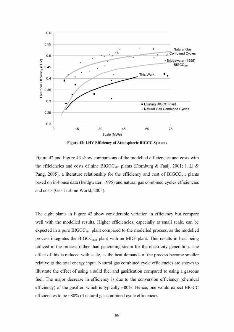
88

0.2

0.25

0.3

0.35

0.4

0.45

0.5

0.55

0.6

0 15 30 45 60 75Scale (MWe)

Electr

ical E

fficien

cy (L

HV)

Existing BIGCC PlantNatural Gas Combined Cycles

Natural Gas Combined Cycles

Bridgewater (1995)BIGCCatm

This Work

Figure 42: LHV Efficiency of Atmospheric BIGCC Systems

Figure 42 and Figure 43 show comparisons of the modelled efficiencies and costs with the efficiencies and costs of nine BIGCCatm plants (Dornburg & Faaij, 2001; J. Li & Pang, 2005), a literature relationship for the efficiency and cost of BIGCCatm plants based on in-house data (Bridgwater, 1995) and natural gas combined cycles efficiencies and costs (Gas Turbine World, 2005).

The eight plants in Figure 42 show considerable variation in efficiency but compare well with the modelled results. Higher efficiencies, especially at small scale, can be expected in a pure BIGCCatm plant compared to the modelled process, as the modelled process integrates the BIGCCatm plant with an MDF plant. This results in heat being utilized in the process rather than generating steam for the electricity generation. The effect of this is reduced with scale, as the heat demands of the process become smaller relative to the total energy input. Natural gas combined cycle efficiencies are shown to illustrate the effect of using a solid fuel and gasification compared to using a gaseous fuel. The major decrease in efficiency is due to the conversion efficiency (chemical efficiency) of the gasifier, which is typically ~80%. Hence, one would expect BIGCC efficiencies to be ~80% of natural gas combined cycle efficiencies.

89

The trend evident from Figure 43 is that at small scale BIGCC plants are very expensive. Costs from existing plants suggest that Bridgewater’s and the modelled relationship may be overstating costs. The costs derived from the model are likely to have an uncertainty of ±30%.

$0

$2,000

$4,000

$6,000

$8,000

$10,000

$12,000

0 10 20 30 40 50 60Scale (MWe)

Spec

ific C

apita

l Cos

t (NZ2

005$

/kWel)

Existing BIGCC Plant

Bridgewater (1995)BIGCCatm

This Work

Figure 43: Capital Cost of BIGCC Plant

The scale of these capital costs counts strongly against the economic appeal of BIGCC systems. Over a 30 yr operating life and with cost of capital of 10% a BIGCC system is uneconomic for all power outputs. The appeal (NPV) of a BIGCC system decreases with scale as shown in Figure 44. However, the breakeven electricity price also decreases with scale. This suggests that at current electricity prices large BIGCC plants will lose more money than small BIGCC plants but, if electricity prices increased, BIGCC plants would become economic first at large scales. For a breakdown of the capital cost of a BIGCC plant refer to Appendix C.

90

-150

-120

-90

-60

-30

0

30

60

90

120

150

0 10 20 30 40 50 60 70Scale (MWe)

NPV (

$M)

-0.25

-0.2

-0.15

-0.1

-0.05

0

0.05

0.1

0.15

0.2

0.25

Brea

keve

n Elec

tricity

Price

($/kW

h)

NPV

Electricity Price

Figure 44: Net Present Value of BIGCC Projects

10.1.3 Sensitivity Analysis

A sensitivity analysis for the BIGCC process, see Figure 45 and Figure 46, shows that the major factors affecting the economics of the project are the capital cost, of which the HRSG and gas turbine contribute over 50%, and gas turbine efficiency. Figure 30 shows that there is considerable difference in the efficiency of turbines on the market; therefore, careful selection of turbine is important. Electricity price has a lesser impact on the economics and, as fuel is cheap, fuels costs have a negligible effect on the project.

91

-90

-80

-70

-60

-50

-40

-30

-20

-10

0-30.00% -20.00% -10.00% 0.00% 10.00% 20.00% 30.00%

Percentage Change from Base CaseNP

V ($M

) Gas Turbine EfficiencyElectricity PriceFuel CostsCapital Costs

Figure 45: Sensitivity Analysis for a 15MWe BIGCC Plant

-200

-180

-160

-140

-120

-100

-80

-60

-40

-20

0-30.00% -20.00% -10.00% 0.00% 10.00% 20.00% 30.00%

Percentage Change from Base Case

NPV (

$M) Electricity Price

Gas Turbine EfficiencyFuel CostCapital Cost

Figure 46: Sensitivity Analysis of a 40MWe BIGCC Plant

92

10.1.4 Gas Turbine Topping Cycle

Due to the NPV of BIGCC project decreasing with scale and capital cost being a significant factor in the economics of the projects, the feasibility of using a gasifier-gas turbine cycle was investigated. The gas turbine offers efficiencies of around 20-25% on producer gas and exhausts waste heat at high temperature, which is a good match for the process heat demands of an MDF plant.

10.1.5 Electrical Efficiency and Capital Cost

The electrical efficiency of a gasifier-gas turbine cogeneration plant is comparable to the best combustion-steam turbine process and higher than a typical combustion-steam process. For economic reasons typical combustion-steam turbines plants operate with a steam pressure of 6 MPa and 480°C, which result in efficiencies of 14-18% (Williams & Larson, 1996). Hence, the average gasifier-gas turbine project offers five to ten efficiencies points on the average combustion steam turbine project. However, the capital costs are still large at $4400/kWel to $5500/kWel over 6-12 MWel range.

0

1000

2000

3000

4000

5000

6000

7000

6 7 8 9 10 11 12Scale (MWe)

Spec

ific C

apita

l Cos

t ($/kW

el)

20%

21%

22%

23%

24%

25%

26%

27%

28%

29%

30%

Electr

ical E

fficien

cy (L

HV)

Capital CostEfficiency

Figure 47: Efficiency and Capital Cost of Gasifier-Gas turbine Projects

93

The feasibility of a gasifier-gas turbine project is significantly greater than a BIGCC project; however, it still does not make economic sense as it has a negative NPV over the entire scale range studied, see Figure 48. Unlike the BIGCC system, the gas turbine project exhibits an increasing break-even electricity price. Therefore, while a BIGCC is most likely to become economic first at a large scale, the gas turbine cycle will become economic first at a small scale.

-12-10-8-6-4-202468

1012

6 7 8 9 10 11 12Scale (MWe)

NPV (

$M)

-0.12-0.1-0.08-0.06-0.04-0.0200.020.040.060.080.10.12

Brea

keve

n Elec

tricity

Price

($/kW

h)

NPV

Electricity Price

Figure 48: NPV and Breakeven Electricity Price of Gasifier-Gas Turbine Projects

10.1.6 Discussion of BIGCC Plant Economics

The ideology of a biomass integrated combined cycle plant is appealing. Biomass gasification combined cycle offers the world a high technology, high-efficiency renewable generation option. It increases the resource efficiency of the nation by using a fuel which is often waste and reduces our fossil fuel dependence by offering a carbon neutral base-load generation technology. However, BIGCC does not utilise the advantages of gasification. Primarily gasification is an enabling technology for gas turbine and gas engine power generation fuelled by biomass, which is presumably in plentiful supply and cheap. In order for the additional step of gasifying a fuel to be economically viable, the additional capital costs of the gas turbine/engine process has to be justified by the gains from increased efficiency. Increased efficiency gains are fuel

94

savings. When the cost of fuel is low, as is the case with biomass, fuel savings are less important. For instance, installing a natural gas combined cycle process instead of the simpler natural gas turbine process is economically appealing when the price of natural gas is above ~$4/GJ based on assuming the two systems have similar installation costs2. If the gasification and associated units increased the cost of each process equally, then there is a $4/GJ hurdle which fuel costs need to exceed for combined cycles to be favoured over gas turbine only cycles. This analysis takes no heed of the higher value heat provided by a gas turbine cycle and compares the relative merits of gas turbine cycles against combined cycles. It does not speak for the economics of each process individually. Unfortunately for biomass gasification, the economics of both are not favourable. The net present value for a BIGCC project is negative for all power ranges and increases with decreasing scale. However, the breakeven electricity price is lowest at higher scale. Electricity costs would have to increase to 14 c/kWh for large scale BIGCC plants to be economically viable. Small scale gasifier-gas turbine plants are a more appealing option but the electricity price still needs to increase to 8-10 c/kWh for these plants to be economic.

2 See Appendix B.8 for method and assumptions

95

10.2 Gasifier-Gas Engine

10.2.1 Introduction

A gasifier gas-engine offers a modular approach to power generation. Gas turbines vary in size from hundreds of kilowatts (electric) up to hundreds of megawatts (electric), while the largest gas engine produced by Jenbacher is only four megawatts (electric). At this scale, gas turbines have lower efficiency than gas engines and generally higher capital cost (Brammer & Bridgwater, 2002). Increasing the scale of gasifier-gas engine plants beyond 3.8 MWel requires the use of multiple engines and, hence, beyond 3.8 MWel there are no gains in engine efficiency with increased scale. Another feature of gas engines is the requirement for cooling. Gas engines produce a large amount of low-grade heat, often in the form of hot-water, for which an MDF plant has minimal need. Gas engines are appealing at smaller scales than gas turbines and, therefore, it becomes necessary to have the gas engine in parallel with a boiler system in order to meet the heat requirements of the MDF plant. Only above 18MWel does the gas engine exhaust have sufficient sensible heat to meet the heat demands of the MDF plant.

Also, unlike the BIGCC system which has an HRSG which can be supplementary fired if the gas turbine was not in operation, a gas engine system may require a boiler capable of meeting the full heat demand of the plant if the availability and reliability of the gas engine is not acceptable.

96

10.2.2 Electrical Efficiency and Capital Cost

Figure 49 and Figure 50 show the efficiency and capital cost of gasifier-gas engine plants and a comparison against reported values in the literature. Efficiencies and costs for existing plant are extracted from Dornburg and Faaij (2001), Brammer and Bridgewater (2002) and Li and Pang (2005) and the literature relationship is courtesy of Bridgewater (1995). Electrical efficiencies (electrical output of the engine divided by total thermal input into the gasification plant) are shown in Figure 49 for a stand-alone gas engine plant (model – no heat plant) and for a gas engine plant integrated into an MDF plant (model). Integration into an MDF plant reduces the electrical efficiency at small scales due to a large proportion of the product gas going to the boiler, rather than the engine, in order to meet the heat demand from the MDF plant. At scales above 18.1MWel the efficiencies of the integrated plant are equal to the stand-alone plant as the gas engine exhaust is sufficient to meet all the plants heat demand. The modelled efficiencies of a stand-alone engine plant are similar to existing plants and higher than those reported by Bridgewater (1995). Bridgewater reports a general relationship for gasifier-gas engine plants which assumes that the product gas is from air-blown gasification and, therefore, it is likely that the relationship assumes a de-rating of the gas engine due to lower calorific value of the air-blown gasification product gas. Furthermore, the modelled relationship is based on Jenbacher engines, due to their experience with FICFB gas, and Jenbacher engines represent the high efficiency end of the market. Figure 50 shows the capital cost trends for gasifier-gas engine plant. Two modelled costs are shown. The more expensive trend (Full-Load Boiler) assumes that, in order to guarantee heat supply to the MDF plant, a boiler capable of meeting the full heat demand is required. This implies that the gas engine will not operate reliably enough for the sensible heat in its exhaust gas to be guaranteed. The cheaper trend (Reliable Gas-Engine) assumes that the boiler needs only be sized to meet the MDF heat demand less the sensible heat in the gas engine exhaust stream.

97

0%

5%

10%

15%

20%

25%

30%

35%

40%

0 5 10 15 20 25 30Scale (MWe)

Effic

iency

(LHV

)

Actual Plants

Bridgwater (1995)

Model

Model - No heat plant

Engin

e me

ets he

at de

mand

Figure 49: Gasifier-Gas Engine Efficiency

Figure 50: Gasifier-Gas Engine Capital Cost

Figure 50 shows that the modelled capital costs exhibit similar trends to existing plant and Bridgewater’s relationship except for at small scales. However, at small scales it is not reasonable to compare capital costs on a $/kWel as the modelled plants are at this scale primarily heat plants. For a breakdown of the capital cost refer to Appendix C.

98

10.2.3 Economics

Figure 51 and Figure 52 show the net present value of the two gasifier-gas engine projects and the break-even electricity price. Gasifier-gas engine projects have a positive NPV in the range from 0 to 30 MWel. The fact that the NPV is positive at a scale of zero MWel shows that a gasifier-gas boiler system without a gas engine is an economic option. Increasing the size of the engine up to 4.79 MWel increases the NPV at an increasing rate. At 4.79 MWel, the plant is sized to meet the total internal electricity demand of the plant. Beyond this scale, the extra electricity generated must be sold at the lower exported electricity price. Increasing the scale of the plant so that it is exporting electricity does not significantly affect the NPV of the system without a full-load bypass boiler. This is due to the increase in capital costs of the gas engine, due to increasing the size of the engine, being partially compensated by decreasing capital costs of the gas-boiler, due to decreasing the size of the boiler. This occurs up until the plant is generating 18 MWel of electricity. At 18 MWel the sensible heat from the engine exhaust can meet the full heat demand of the plant and no boiler is required. Therefore, increasing the scale of the plant beyond 18 MWel results in a steadily decreasing NPV as there is no compensating decrease in gas-boiler costs with increasing gas engine scale. If the gas engine exhaust heat cannot be relied upon, then there is no compensating decrease in gas-boiler costs at any scale of gas engine. Figure 51 shows that there is a significant economic advantage in having a reliable gas engine. The additional costs of having a boiler capable of meeting the full heat-load of the process, as opposed to the full heat load less the heat supplied by a reliable engine, significantly reduces the NPV of project. This is particularly evident at larger scales. 4.79 MWel is shown by Figure 51 to be the most appealing scale for a gasifier-gas engine plant. However, for a plant with a reliable engine, the NPV is similar for scales from 4.79MWel to 18.1MWel, but the break-even price and sensitivity analysis shows that the 4.79MWel plant is a less risky project.

99

-$15

-$10

-$5

$0

$5

$10

$15

0 5 10 15 20 25 30Scale (MWe)

NPV (

$M)

Intern

al Ele

ctricit

y Req

uirem

ents

Gas E

ngine

Mee

ts He

at De

mand

Without boiler capable of meeting full heat demand

With boiler capable of meeting full heat demand

Figure 51: NPV of Gasifier-Gas Engine System

$0.00

$0.01

$0.02

$0.03

$0.04

$0.05

$0.06

$0.07

$0.08

$0.09

$0.10

0 5 10 15 20 25 30Scale (MWe)

Brea

keve

n Elec

tricity

Price

($/kW

h)

Intern

al Ele

ctricit

y Req

uirem

ents

Heat

Prod

uctio

n Exc

eeds

Dem

and

Without boiler capable of meeting full heat demand

With boiler capable of meeting full heat demand

Figure 52: Breakeven Electricity Price of Gasifier-Gas Engine System

100

At this point the advantage of integrating with an MDF plant should be noted. The MDF plant provides the process with $3.4M annually for the heat provided. The net present value of this over the 30 year life of the plant is $32.5M. Removing $32.5M from the NPV makes the project economics look very unfavourable. Hence recognition of the value of the heat provided by the process is essential for economics of gasification to be favourable. This is mentioned here and not earlier because, even with the recognition of the value of heat, the project economics for the gasifier-gas turbine and BIGCC project are unfavourable. Another factor to be aware of in the favourable economics presented here is that the MDF plant consumes 4.79 MW of electricity internally. Internally consumed electricity is more valuable than exported electricity as the avoided cost of using in-house generation to meet internal demand is greater than the price received from exporting electricity due primarily to lines charges and losses. The 1.6 c/kWh premium received for electricity consumed internally results in $620,000 in additional annual revenue which has a present value over the 30 year life of the plant of $5.8M. A gasifier-gas engine plant sized to meet the internal electricity demands of the MDF plant has a breakeven electricity price well below the current 8 c/kWh and therefore could economically produce electricity even if electricity prices dropped considerably. Larger scales have higher breakeven electricity prices and at 18MWel the breakeven price approaches the lower bound of current fixed price electricity contracts. The NPV’s are similar due to the increased volume of electricity sold at larger scales but the margins are lower and therefore the project is more risky.

10.2.4 Sensitivity Analysis

Figure 53 and Figure 54 show a sensitivity analysis of gasifier-gas engine plant at two different scales. At 4.79 MWel the analysis shows that the project maintains its economic appeal when capital cost, electricity price and fuel cost are altered by ±30%. At a larger 18.1 MWel scale, the estimate NPV for the base case is similar but the project is much more sensitive to changes in electricity price and capital cost. This sensitivity analysis shows that the smaller plant is a safer project but the larger project

101

has more scope for high returns if electricity prices rise or capital costs drop and more scope for loss if electricity prices fall or capital cost rise.

0

2

4

6

8

10

12

14

16

18

-40% -30% -20% -10% 0% 10% 20% 30% 40%Percentage Change from Base Case

NPV (

$M) Capital Costs

Electricity PriceFuel Cost

Figure 53: Sensitivity Analysis of a 4.79MWel Gasifier-Gas Engine Plant

-15

-10

-5

0

5

10

15

20

25

30

35

-40% -30% -20% -10% 0% 10% 20% 30% 40%Percentage Change from Base Case

NPV (

$M) Electricity Price

Fuel CostCapital Cost

Figure 54: Sensitivity Analysis of an 18.1MWel Gasifier-Gas Engine Plant

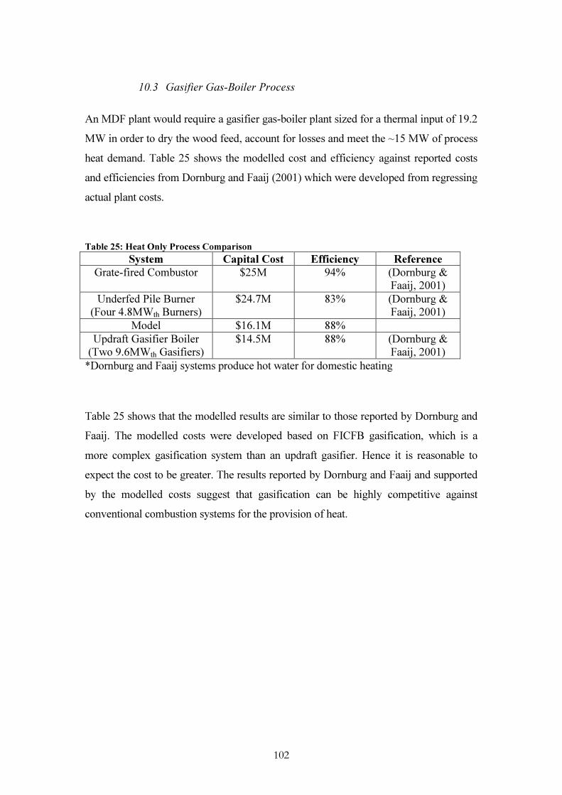
102

10.3 Gasifier Gas-Boiler Process

An MDF plant would require a gasifier gas-boiler plant sized for a thermal input of 19.2 MW in order to dry the wood feed, account for losses and meet the ~15 MW of process heat demand. Table 25 shows the modelled cost and efficiency against reported costs and efficiencies from Dornburg and Faaij (2001) which were developed from regressing actual plant costs. Table 25: Heat Only Process Comparison

System Capital Cost Efficiency Reference Grate-fired Combustor $25M 94% (Dornburg &

Faaij, 2001) Underfed Pile Burner

(Four 4.8MWth Burners) $24.7M 83% (Dornburg &

Faaij, 2001) Model $16.1M 88%

Updraft Gasifier Boiler (Two 9.6MWth Gasifiers)

$14.5M 88% (Dornburg & Faaij, 2001)

*Dornburg and Faaij systems produce hot water for domestic heating Table 25 shows that the modelled results are similar to those reported by Dornburg and Faaij. The modelled costs were developed based on FICFB gasification, which is a more complex gasification system than an updraft gasifier. Hence it is reasonable to expect the cost to be greater. The results reported by Dornburg and Faaij and supported by the modelled costs suggest that gasification can be highly competitive against conventional combustion systems for the provision of heat.

103

10.4 Perspective

At this stage, it is important to put some perspective on the projects that have been presented in this thesis. Currently, New Zealand has two biomass electricity generation facilities bigger than 10MWel in Kinleith and Pan Pac. These are 40 MWel and 13 MWel respectively (Dang, 2005). This shows that projects of similar scale to those discussed in this thesis have been undertaken in New Zealand. However, at scales of 55MWel a 120,000 m3/yr MDF plant would be making the same amount of gross revenue from exporting electricity as they would be exporting MDF. This is based on an MDF export price of $US200/m3 (Chapman K, pers. comm.). This puts a distinct perspective on integrating a BIGCC scale system with an MDF plant. The MDF plant would no longer be a wood processor but equal parts wood processor and electricity generator. Moreover, the capital required for a 55 MWel plant would be the equivalent of seven years of gross revenue from selling MDF. On the other hand, gross revenue from selling electricity from a 5 MWel gas engine scale plant would be equivalent to 9% of the MDF gross revenue and the capital cost would be less than one year of gross MDF revenue. Overall the 5 MW gas engine project is still a very substantial project for an MDF plant, but it is a significantly more viable project than a 55 MWel BIGCC project.

104

11 Conclusions

The BIGCC system is uneconomic in the current economic environment. An electricity price in excess of 14 c/kWh is required in order to attract investment in this technology. The large capital costs prevent the process from being economically feasible. The capital costs need to be reduced for this process to compete with the gas engine process. The gas turbine and heat recovery steam system are the major capital costs. Reduction in the costs of these two components is required before this technology can become feasible. Further research into the additional costs of utilizing wood producer gas in gas turbines may reduce the cost of this process. The breakeven electricity price for BIGCC systems decreases with scale and, therefore, if a BIGCC project was undertaken it is likely to be of large scale. The gas turbine process is uneconomic in the current economic environment. However, the economics are better than the BIGCC process showing that removing the steam cycle improves the economics considerably. This is evidence that the steam cycle capital costs are a major factor preventing the appeal of BIGCC systems. A gasifier-gas turbine process, which is sized so that all exhaust heat is used in the process, is very close to having a positive NPV and, therefore, shows some appeal. The breakeven electricity price is just over eight c/kWh and, therefore, any increase in electricity prices would make the project marginally feasible. The efficiency of the gas turbine has a large effect on the economics of the project so careful selection of the gas turbine is important. Gas turbines have a wide variation in efficiency. The gasifier-gas engine process is an economic process and easily the most appealing. A gasifier-gas engine process sized to meet the internal electricity demands of the process has the most positive NPV and sensitivity analysis shows that the NPV remains positive when electricity price, capital cost and wood cost is altered by ±30%. This indicates that the process is economic over a wide range of conditions. A larger gasifier-gas engine plant is more dependent on having a reliable engine (therefore not requiring a boiler capable of meeting the full heat demand of the process) and more sensitive to electricity price and capital cost. However, there is significantly more potential for high

105

returns if electricity price increases, as is the long-term trend. Research into the increase in capital cost and decrease in efficiency, due to the high hydrogen content of the gas needs to be undertaken to verify these conclusions. Smith, Fairclough et al.’s (2003) generation costs for the primary substitutes of biomass gasification power generation, shown in Table 26, show that the gasifier-gas engine process is very appealing and highly competitive, the gasifier-gas turbine has marginal appeal and the BIGCC system has little appeal and is not competitive. Table 26: Comparison of Gasification Electricity Costs with substitutes

Generation Type Cost (c/kWh) Gasifier-Gas Engine 4.0 to 9.0 Gas Combined Cycle 5.7 to 7.7

Wind 6.2 to 8.5 Geothermal 4.01 to 8.5

Coal 6.1 to 7.1 Hydro 7.0 to 8.5

Gasifier-Gas Turbine 8.0 to 11.2 Liquefied Natural Gas 8.5 to 10.6

Fuel Oil 11.3 BIGCC 14 to 25 Distillate 16.0

1 Only an estimated 25MW exist at the 4.0 c/kWh cost, after that geothermal is expected to cost 7.0 c/kWh. When considering the contents of Table 26 is important to remember the influence integration with an MDF has on the project. Integration with an MDF plant gives cash flows worth $38M (present value) over the life of each electricity generating project. This benefit is derived from the value of the heat produced and the difference between the avoided cost of purchasing electricity and price received for exporting electricity. The gasifier-gas boiler process also shows considerable appeal and comparison with costs published by Dornburg and Faaij (2001) show that gasification can compete well against conventional combustion systems.

106

12 Recommendations

Modelling of FICFB gasification can be improved beyond what is possible with chemical equilibrium through taking a reaction rate approach. However, the effort involved in developing such a model is not likely to be justified if it is for the sole purpose of preliminary economic analysis. It is recommended that, for further economic analysis, experimental results for the product gas composition for FICFB gasification be used. However, this cannot occur until product gas compositions are known for the desired operating conditions. Reaction rate modelling of FICFB gasification is an area which has significant potential for furthering the understanding of the FICFB process. A computational fluid dynamics model, which can incorporate solid particles, would be highly beneficial in designing pilot FICFB plant. Such a study represents an ideal opportunity for PhD study within the BIGAS consortium. In the short-term, a useful experimental run would be to investigate the product gas composition of FICFB gasification under a nitrogen (non-reacting) environment. This would inform the consortium about fast devolatilisation in FICFB gasification and allow discussion on the extent to which char gasification and the homogenous gas-phase reaction take place. In order to complete the goals of objective four of the BIGAS consortium, the economic model has to be widened to include integration with sawmill and laminated veneer lumber (LVL) plants. Once information on the energy demand of these wood processors becomes available from objective three, it is recommended that the model be expanded to include these energy consumers. It should not be a major task to expand the model presented in this thesis to include these energy consumers. The model also needs to be widened to allow selection of geographical area. Currently, wood availability and cost is only available for the Canterbury region and, therefore, the model is restricted to the Canterbury region. Again, when supply cost curves are available from objective three for other regions, it should not be a major task to integrate them into the existing model.

107

13 Final Statement

Biomass gasification is an energy option that holds so much promise. It offers New Zealand a carbon-neutral, renewable, indigenous co-generation energy option that could go far in strengthening New Zealand’s energy security. A security, which is currently weak, and stated in a 2003 New Zealand forest products industry review as a key reason for the lack of recent, and foreseeable, investment in additional MDF capacity in New Zealand (Neilson & Buckleigh, 2003). This thesis set itself the question of whether biomass gasification is economically feasible, for it needs to be economically feasible in order to play a role in New Zealand’s energy future. The conclusions of this thesis state that the choice of process is very important and that a gasifier-gas engine process could be economically viable in the current environment. However, this feasibility comes with a number of caveats. Firstly, the feasibility is dependant on integration with an MDF plant. Recognition of the value of the heat generated in the process and access to a supply of wood feed is critical for the viability of the process. Secondly, a number of technological barriers need to be overcome. The major barriers are whether the gasifier can be run reliably for 8000 hours a year, whether the gas can be cleaned effectively for reliable engine and turbine use, whether the syngas coolers can be used for heat recovery without severe fouling and whether serious modification to the gas engine is required to compensate for the high hydrogen content of the product gas. The basis of the treatment of these issues in this thesis is the experience of the Gussing plant. Therefore, before a firmer estimate of a New Zealand based gasification plant’s feasibility can be made, these issues need to be overcome locally or the engineering expertise of the Gussing plant tapped. Therefore, yes, biomass gasification can play an economically feasible role in the energy future of New Zealand. However, there is still considerable work to be done before this happens.

108

14 References

AIAA. (1998). Guide for the verification and validation of computational fluid dynamics simulations (No. AIAA-G-077-1998): Am. Inst. Aeronaut. Astronaut.

Altafini, C. R., Wander, P. R., & Barreto, R. M. (2003). Prediction of the working parameters of a wood waste gasifier through an equilibrium model. Energy Conversion and Management, 44(17), 2763-2777.

Babu, B. V., & Chaurasia, A. S. (2003). Modeling, simulation and estimation of optimum parameters in pyrolysis of biomass. Energy Conversion and Management, 44(13), 2135-2158.

Baines, J. (1993). New Zealand Energy Information Handbook. Christchurch: Taylor Baines and Associates.

Bilodeau, J.-F., Therien, N., Proulx, P., Czernik, S., & Chornet, E. (1993). Mathematical model of fluidized bed biomass gasification. Canadian Journal of Chemical Engineering, 71(4), 549-557.

Bouman, R. W., Jesen, S., & Wake, M. L. (2004). Process Capital Cost Estimation for New Zealand 2004: Society of Chemical Engineers New Zealand.

Brammer, J. G., & Bridgwater, A. V. (1999). Drying technologies for an integrated gasification bio-energy plant. Renewable and Sustainable Energy Reviews, 3, 243-289.

Brammer, J. G., & Bridgwater, A. V. (2002). The influence of feedstock drying on the performance and economics of a biomass gasifier-engine CHP system. Biomass and Bioenergy, 22(4), 271-281.

Bridgwater, A. V. (1995). The technical and economic feasibility of biomass gasification for power generation. Fuel, 74(5), 631-653.

Brown, J., Dobbs, R., & Gilmore, I. (2006). Biomass Gasification in a Fast Internal Circulated Fluidised Bed Gasifier. Paper presented at the Chemeca, Auckland.

Caputo, C., Palumbo, M., Pelagagge, P., & Scacchia, F. (2005). Economics of biomass energy utilization in combustion and gasification plants: effect of logistic variables. Biomass and Bioenergy, 28, 35-51.

Chemical Engineering.). New York: Chemical Week Associates. Corella, J., & Sanz, A. (2005). Modeling circulating fluidized bed biomass gasifiers. A

pseudo-rigorous model for stationary state. Fuel Processing Technology, 86, 1012-1053.

Coulter, B. (2005, 28th November, 2005). Commercial Application of Thermal Gasification Technologies for Generation of Steam using Wood Wastes. Paper presented at the Biomass Gasification Workshop, University of Canterbury.

Dang, H. (2005). New Zealand Energy Data File July 2005. Wellington: Ministry of Economic Development 2005.

de Souza-Santos, M. (2004). Solid Fuel Combustion and Gasification. Modeling, Simulation and Equipment Operation. New York: Marcel Dekker Inc.

Devi, L., Ptasinski, K. J., & Janssen, F. J. J. G. (2003). A review of the primary measures for tar elimination in biomass gasification processes. Biomass and Bioenergy, 24(2), 125-140.

Dornburg, V., & Faaij, A. P. C. (2001). Efficiency and economy of wood-fired biomass energy systems in relation to scale regarding heat and power generation using combustion and gasification technologies. Biomass and Bioenergy, 21(2), 91-108.

Douglas, J. M. (1988). Conceptual Design of Chemical Processes: McGraw-Hill.

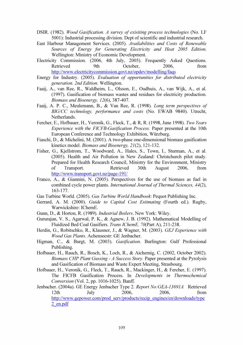
109

DSIR. (1982). Wood Gasification. A survey of exisiting process technologies (No. LF 5001): Industrial processing division. Dept of scientific and industrial research.

East Harbour Management Services. (2005). Availabilities and Costs of Renewable Sources of Energy for Generating Electricity and Heat 2005 Edition. Wellington: Ministry of Economic Development.

Electricity Commission. (2006, 4th July, 2005). Frequently Asked Questions. Retrieved 9th October, 2006, from http://www.electricitycommission.govt.nz/opdev/modelling/faqs

Energy for Industry. (2005). Evaluation of opportunities for distributed electricity generation. 2nd Edition. Wellington.

Faaij, A., van Ree, R., Waldheim, L., Olsson, E., Oudhuis, A., van Wijk, A., et al. (1997). Gasification of biomass wastes and residues for electricity production. Biomass and Bioenergy, 12(6), 387-407.

Faaij, A. P. C., Meulemann, B., & Van Ree, R. (1998). Long term perspectives of BIG/CC technology, performance and costs (No. EWAB 9840). Utrecht, Netherlands.

Fercher, E., Hofbauer, H., Veronik, G., Fleck, T., & R, R. (1998, June 1998). Two Years Experience with the FICFB-Gasification Process. Paper presented at the 10th European Conference and Technology Exhibition, Würzburg.

Fiaschi, D., & Michelini, M. (2001). A two-phase one-dimensional biomass gasification kinetics model. Biomass and Bioenergy, 21(2), 121-132.

Fisher, G., Kjellstrom, T., Woodward, A., Hales, S., Town, I., Sturman, A., et al. (2005). Health and Air Pollution in New Zealand: Christchurch pilot study. Prepared for Health Research Council, Ministry for the Environment, Ministry of Transport. Retrieved 30th August 2006, from http://www.transport.govt.nz/page-191/

Franco, A., & Giannini, N. (2005). Perspectives for the use of biomass as fuel in combined cycle power plants. International Journal of Thermal Sciences, 44(2), 163-177.

Gas Turbine World. (2005). Gas Turbine World Handbook: Pequot Publishing Inc. Gerrard, A. M. (2000). Guide to Capital Cost Estimating (Fourth ed.). Rugby,

Warwickshire: IChemE. Gunn, D., & Horton, R. (1989). Industrial Boilers. New York: Wiley. Gururajan, V. S., Agarwal, P. K., & Agnew, J. B. (1992). Mathematical Modelling of

Fluidized Bed Coal Gasifiers. Trans IChemE, 70(Part A), 211-238. Herdin, G., Robitschko, R., Klausner, J., & Wagner, M. (2003). GEJ Experience with

Wood Gas Plants. Achenseestr: GE Jenbacher. Higman, C., & Burgt, M. (2003). Gasification. Burlington: Gulf Professional

Publishing. Hofbauer, H., Rauch, R., Bosch, K., Loch, R., & Aichernig, C. (2002, October 2002).

Biomass CHP Plant Gussing - A Success Story. Paper presented at the Pyrolysis and Gasification of Biomass and Waste Expert Meeting, Strasbourg.

Hofbauer, H., Veronik, G., Fleck, T., Rauch, R., Mackinger, H., & Fercher, E. (1997). The FICFB Gasification Process. In Developments in Thermochemical Conversion (Vol. 2, pp. 1016-1025). Banff.

Jenbacher. (2004a). GE Energy Jenbacher Type 2. Report No:GEA-13691A Retrieved 12th July 2006, 2006, from http://www.gepower.com/prod_serv/products/recip_engines/en/downloads/type2_en.pdf

110

Jenbacher. (2004b). GE Energy Jenbacher Type 3. Report No:GEA-13690 Retrieved 12th July 2006, 2006, from http://www.gepower.com/prod_serv/products/recip_engines/en/downloads/type3_en.pdf

Jenbacher. (2004c). GE Energy Jenbacher Type 4. Report No:GEA-13691 Retrieved 12th July 2006, 2006, from http://www.gepower.com/prod_serv/products/recip_engines/en/downloads/type4_en.pdf

Jenbacher. (2004d). GE Energy Jenbacher Type 6. Report No:GEA-13692 Retrieved 12th July 2006, 2006, from http://www.gepower.com/prod_serv/products/recip_engines/en/downloads/type6_en.pdf

Jones, R., & Shilling, N. (2003). IGCC Gas Turbines for Refinery Applications (No. GER-4219). Schenectady: GE.

Jones, W., & Lindstedt, R. (1988). Global Reaction Schemes for Hydrocarbon Combustion. Combustion and Flame, 73, 233-249.

Kaiser, S., Weigl, K., Schuster, G., Tremmel, H., Friedl, A., & Hofbauer, H. (2000). Simulation and optimization of a biomass gasification process. Paper presented at the 1st World Conference and Exhibition on Biomass for Energy and Industry, Sevilla.

Kersten, S., Prins, W., van der Drift, A., & van Swaaij, W. (2003). Experimental Fact-Finding in CFB Biomass Gasification for ECN's 500 kWth Pilot Plant. Ind. Eng. Chem. Res, 42(26), 6755-6764.

Kinoshita, C., & Wang, W. (1993). Kinetic Model of Biomass Gasification. Solar Energy, 51(1), 19-25.

Koufopanos, C. A., Papayannakos, N., Maschio, G., & Lucchesi, A. (1989). Kinetic modelling of the pyrolysis of biomass and biomass components. The Canadian J Chem Eng, 67, 75-84.

Li, J., & Pang, S. (2005). Objective 1 Evaluation of BIGCC Technologies Developed Overseas (Literature Reveiw): University Of Canterbury, Department of Chemical and Processing Engineering.

Li, J., & Pang, S. (2006). Modelling of energy demand in a MDF plant. Paper presented at the Chemeca, Auckland.

Li, X., Grace, J. R., Watkinson, A. P., Lim, C. J., & Ergudenler, A. (2001). Equilibrium modeling of gasification: a free energy minimization approach and its application to a circulating fluidized bed coal gasifier. Fuel, 80(2), 195-207.

Li, X. T., Grace, J. R., Lim, C. J., Watkinson, A. P., Chen, H. P., & Kim, J. R. (2004). Biomass gasification in a circulating fluidized bed. Biomass and Bioenergy, 26(2), 171-193.

Liliedahl, T., & Sjostrom, K. (1997). Modelling of char-gas reaction kinetics. Fuel, 76(1), 29-37.

Liu, H., & Gibbs, B. M. (2003). Modeling NH3 and HCN emissions from biomass circulating fluidized bed gasifiers*. Fuel, 82(13), 1591-1604.

Major, G. (1995). Learning from experiences with small-scale cogeneration (Revised 1995 ed.). Sittard: CADDET.

Maloney, T. (1993). Modern Particleboard and Dry-process Fiberboard Manufacturing. San Francisco: Miller Freeman.

Marsden, A., Poskitt, R., & Small, J. (2004). Investment in the New Zealand Electricity Industry. A examination of comparative finanical performance, pricing and new

111

entry conditions; and a discussion of the principles of new investment. Auckland: Auckland UniServices Limited.

Massardo, A., & Scialo, M. (2000). Thermoeconomic Analysis of Gas Turbine Based Cycles. J Eng Gas Turbines and Power, 122, 664-671.

Ministry of Agriculture and Forestry. (2004). A National Exotic Forest Description as at 1st April 2004 (No. Ed 21).

Miura, K., Hashimoto, K., & Silveston, P. L. (1989). Factors affecting the reactivity of coal chars during gasification, and indices representing reactivity. Fuel, 68(11), 1461-1475.

Neilson, D., & Buckleigh, D. (2003). The New Zealand Forest Products Industry Review 2003 Edition. Rotorua: DANA Publishing.

Pang, S. (2005, 28th Nivember 2005). From Residues to Energy: Research Programme on Woody Biomass Integrated Gasification Applied Systems (BIGAS). Paper presented at the CAE. Biomass Gasification Workshop, University of Canterbury.

Pfeifer, C., Rauch, R., & Hofbauer, H. (2004). In-Bed Catalytic Tar Reduction in a Dual Fluidized Bed Biomass Steam Gasifier. Ind. Eng. Chem. Res., 42, 1634-1640.

Rabou, L. P. L. M., & Jansen, D. (2001). De-centralised power production using low-calorific value gas from renewable energy resources in gas turbines (No. ECN-C--01-056): For NOVEM by ECN and OPRA.

Rauch, R. (2006a). Gas Cleaning for gas engine and synthesis gas applications. Paper presented at the IEA Task 33. Thermal Gasification of Biomass. Spring 2006, Dresden.

Rauch, R. (2006b, 30th June 2006). Results from Gasification Tests. . Retrieved 31st August 2006, from www.ficfb.at

Reserve Bank of New Zealand. (2006, 31 August 2006). B1 Exchange Rates. Retrieved 31 August 2006, from http://www.rbnz.govt.nz/statistics/exandint/b1/data.html

Rodrigues, M., Faaij, A. P. C., & Walter, A. (2003). Techno-economic analysis of co-fired biomass integrated gasification/combined cycle systems with inclusion of economies of scale. Energy, 28(12), 1229-1258.

Scharpf, E., & Carrington, G. (2005). Wood-derived producer gas cleanup and tolerances. Dunedin: Delta S Technologies, University of Otago.

Schuster, G., Loffler, G., Weigl, K., & Hofbauer, H. (2001). Biomass steam gasification - an extensive parametric modeling study. Bioresource Technology, 77(1), 71-79.

Smith, A., Fairclough, R., SriRamaratnam, R., Truyens, S., Wilkinson, D., & Little, N. (2003). New Zealand Energy Outlook to 2025. Wellington: Ministry of Economic Development Energy Modelling and Statistics Unit.

Smith, J., Van Ness, H., & Abbott, M. (1996). Introduction to Chemical Engineering Thermodynamics (5th ed.): McGraw-Hill International Editions.

Sonntag, R., Borgnakke, C., & Van Wylen, G. (1998). Fundamentals of Thermodynamics: John Wiley & Sons Inc.

The Marketplace Company. (2006). Comit Free to Air. Retrieved 2nd July 2006, from http://www.comitfree.co.nz/fta/ftapage.main

Transpower. (2004). Future of the National Grid. Discussion Document No 2. Wellington.

Traverso, A., Cazzola, W., & Lagorio, G. (2004, 14-17 June 2004). Widget-Temp: A novel web-based approach for thermoeconomic analysis and optimization of

112

conventional and innovative cycles. Paper presented at the ASME-IGTI Turbo Expo, Vienna.

TRC. (1994). Thermodynamic Properties of Substances in Ideal Gas State. Linear and non-linear coefficients and computer code to regenerate the values of thermodynamic properties. Thermodynamic Research Center. Texas Engineering Experiment Station. Texas.

Ulrich, G. D., & Vasudevan, P. T. (2005). Chemical Engineering. Process Design and Economics. A Practical Guide. (2nd ed.). New Hampshire: Process Publishing.

Wereko-Brobby, C., & Hagan, E. (1996). Biomass Conversion and technology. Chichester, New York: Wiley.

Williams, R. H., & Larson, E. D. (1996). Biomass gasifier gas turbine power generating technology. Biomass and Bioenergy, 10(2-3), 149-166.

Yu, Q., Brage, C., Chen, G., & Sjostrom, K. (1997). Temperature impact on the formation of tar from biomass pyrolysis in a free-fall reactor. Journal of Analytical and Applied Pyrolysis, 40-41, 481-489.

Zainal, Z. A., Ali, R., Lean, C. H., & Seetharamu, K. N. (2001). Prediction of performance of a downdraft gasifier using equilibrium modeling for different biomass materials. Energy Conversion and Management, 42(12), 1499-1515.

113

Appendix A. Gasification Modelling

Appendix A

114

A.1 CRL Energy Ltd Pine Chemical Analysis

INTERIM REPORT OF ANALYSIS Page 1 of 1

Date Received: 26-Aug-05Client: Canterbury UniversityDescription: Wood Chip pellets and Husk samples supplied by client.

CRL Energy Ltd Reference: 76/050 76/051 76/052

Customer Reference:Sample#1 Chips

Sample#2 Pellets Sample#3 Husks

Analysis - As Received Basis

Moisture ISO 5068 % 52.6 8.0 9.9Ash ASTM D1102 % 0.2 0.4 2.6Volatile ISO 562 % 39.8 77.4 73.8Fixed Carbon By Difference % 7.4 14.2 13.7Gross Calorific Value ISO 1928 MJ/kg 9.53 18.63 17.08Carbon micro analytical % 24.3 47.2 43.7Hydrogen micro analytical % 2.87 5.35 5.07Nitrogen micro analytical % <0.1 <0.2 0.56Sulphur ASTM D4239 % 0.01 0.01 0.06Oxygen By Difference % 20.0 38.7 38.1CHN determined by Chemsearch Otago UniversityAnalysis - Dry BasisAsh ASTM D 1102 % 0.4 0.4 2.9Volatile ISO 562 % 84.0 84.1 81.9Fixed Carbon By Difference % 15.6 15.4 15.2Gross Calorific Value ISO 1928 MJ/kg 20.10 20.25 18.95Carbon micro analytical % 51.2 51.3 48.5Hydrogen micro analytical % 6.10 5.81 5.63Nitrogen micro analytical % <0.2 <0.2 0.62Sulphur ASTM D4239 % 0.02 0.01 0.07Oxygen By Difference % 42.3 42.4 42.9

Signature:Date of Issue: 13-Oct-05 Grant Murray

Laboratory SupervisorTHIS REPORT MUST NOT BE QUOTED EXCEPT IN FULLDistribution:Dept of Chemical and Process Engineering, PB 4800, CHCH ATTN: Ian GilmourCRL Energy Ltd, Laboratory

68 Gracefield Road,PO Box 31-244, Lower Hutt, New Zealand TELEPHONE +64 4 570 3700 FACSIMILE +64 4 570 3701

Appendix A

115

A.2 Gasifier Mass Balance Equations

The mass balances for molar carbon, hydrogen and oxygen, equations A.1-A.3 respectively, can be written in the form of an augmented matrix.

(A.1)

(A.2)

(A.3)

4 2

4 2 2

2 2

CH CO wood

CH wood steam moisture

CO wood steam moisture

N N 0 0 NH4N 0 0 2 2 N +2N +2NCO0 2N 0 N +N +NC

CO char

H H O

CO H O

N N

N N

N N

−

wood

wood steam moisture

wood steam moisture

1 1 1 0 0 NH4 0 0 2 2 N +2N +2NCO0 1 2 0 1 N +N +NC

charN −

This can then be reduced to form three linear equations which show the relationship between the molar flows of the carbon gases (CH4, CO & CO2) and the molar flows of water and hydrogen. Action: Row 2 – 4 Row 1

[ ]wood

wood steam moisture wood

wood steam moisture

1 1 1 0 0 N -H0 4 4 2 2 N +2N +2N 4 N -C

O0 1 2 0 1 N +N +NC

char

char

N

N

− − −

4 2

4 2 2

2 2

wood CH CO

wood steam moisture CH

wood steam moisture CO

N = N +NH N +2N +2N = 4N 2 2CO N +N +N = 2NC

char CO

H O H

CO H O

N N

N N

N N

− +

+ +

+ +

Appendix A

116

[ ] [ ]

2 2

2 2

2 2

2

steam moisture4 wood

wood wood steam moisture

steam moisturewood

N +N1 H N +4 C 2 2

1 H O2 N - N -2 N +N 22 C C

33N +3NO 1 H -1 N +C 4 C 2 2

H H OCH

CO char H H O

H H OCO char

N NN

N N N N

N NN N

+= − = − + + +

+ = + + −

Action: Row 2/-4

[ ]wood

wood wood steam moisture

wood steam moisture

1 1 1 0 0 N -H0 1 1 1/ 2 1/ 2 N - N +2N +2N / 4C

O0 1 2 0 1 N +N +NC

char

char

N

N

− − −

Action Row 1 – Row 2 and Row 3 – Row 2

[ ][ ]

wood steam moisture

wood wood steam moisture

wood steam moisture wood wood steam moisture

H1 0 0 1/ 2 1/ 2 N +2N +2N / 4C

H0 1 1 1/ 2 1/ 2 N - N +2N +2N / 4C

O H0 0 1 1/ 2 3/ 2 N +N +N N - N +2N +2N / 4C C

char

char

N

N

− − − − +

Action Row 2 – Row 3

[ ] [ ]wood steam moisture

wood wood steam moisture wood steam moisture wood wood steam moisture

wood steam m

H1 0 0 1/ 2 1/ 2 N +2N +2N / 4C

H O H0 1 0 1 2 N - N +2N +2N / 4 N +N +N N - N +2N +2N / 4C C C

O0 0 1 1/ 2 3/ 2 N +N +NC

char charN N

− − − − + −

[ ]oisture wood wood steam moistureHN - N +2N +2N / 4CcharN

− +

Which yields the following equations:

[ ] [ ]

2 2

2 2

2 2

2

4 wood steam moisture

wood wood steam moisture wood steam moisture wood wood steam moisture

H N +2N +2N / 42 C

H O H2 N - N +2N +2N / 4 N +N +N N - N +2N +2N / 4C C C

3

H H OCH

CO H H O char char

H HCO

N NN

N N N N N

N NN

+ + = − − = − − + −

++ [ ]wood steam moisture wood wood steam moistureO HN +N +N N - N +2N +2N / 4

2 C CO

charN = − + Which can be simplified to:

(A.4)

(A.5)

(A.6) Equation A.6 can be rearranged to derive the molar flow of solid carbon (Nchar), shown in equation A.7, as discussed in section 4.5. (A.7) 2 2

2

steam moisture( ) wood

33N +3NO 1 H -1 NC 4 C 2 2

H H Ochar s CO

N NN NC N

+ = = − + − +

Appendix A

117

A.3 Chemical Equilibrium Calculation

Chemical Equilibrium constants can be derived from fundamental chemical properties using the following relationship. (A.8)

0G-RT

InK ∆= The change in Gibbs energies for a reaction can be calculated by summing the individual Gibbs energies of each species multiplied by the stoichiometric coefficient of the reaction for that species. (A.9) 0 0

i iG Gν∆ =∑ This is the method used in the gasification modelling presented in this thesis. Standard state Gibbs energies from the TRC Tables (1994) are used in the calculation of chemical equilibrium.

Appendix A

118

A.4 Heat Capacity

Heat capacity for a particular species varies with temperature. Therefore, in order to accurately calculate the enthalpy changes in the system, this dependence of heat capacity on temperature needs to be recognized. The literature suggests using the following correlations for heat capacities: (A.10) ( )2 2( )

2 3reaction amb i i

i i i reaction reaction amb ambreaction amb

T T C DCP R A B T T T TT T

+= + + + + +

(Zainal, Ali, Lean, & Seetharamu, 2001)

Where the constants Ai, Bi, Ci and Di can be found in thermodynamic tables and are given below: A 103B 106C 10-5D Methane 1.702 9.081 -2.164 - Hydrogen 3.249 0.442 - 0.083 Carbon Monoxide 3.376 0.557 - -0.031 Carbon Dioxide 5.457 1.047 - -1.157 Nitrogen 3.280 0.593 - 0.040 Water 3.470 1.450 - 0.121 Carbon (graphite) 1.771 0.771 - -0.867 Oxygen 3.639 0.506 - -0.227 These constants are valid up to at least 1500˚K and were extracted from Smith, Van Ness et al. (1996) This equation can be rearranged (A.11) (A.12) Heat capacity of sand was extracted from Sonntag, Borgnakke et al. (1998) and assumed to be constant with temperature. Heat Capacity of Sand = 0.8 kJ/kg/K. .

2 2

2

12 3 2 3 3

i i amb i i i amb i ii amb reaction reaction

amb reaction

ii i i i

CP BT C B CT C DA T T TR T T

dCP a bT cTT

= + + + + + + = + + +

Appendix A

119

A.5 Gasification Model Software

The gasification software model, based on the equations presented in section 4, uses Microsoft Excel. The model consists of eight worksheets inside one spreadsheet. The screenshots of the major worksheets are presented in Figures 55 to 59 and a synopsis of each major worksheet is given. The model calculates chemical equilibrium and an energy balance for a FICFB gasifier. The model can easily be adapted for calculating chemical equilibrium for updraft gasification and the concepts also apply to calculating an energy balance for an updraft gasifier. HYSYSExcelLink This worksheet is the worksheet which acts to pass information between the chemical equilibrium gasification model and the HYSYS process flow schemes. No calculations are performed inside this worksheet. This sheet is only an intermediary between HYSYS and the gasification calculation sheets.

Figure 55: HysysExcelLink

Appendix A

120

Input Sheet The input sheet is a critical worksheet. This is where the user can input the gasification characteristics. Chemical equilibrium is calculated for a stated BFB temperature (this can be substituted for bed temperature when applying the model to an updraft gasifier) and varying ratios of carbon, hydrogen and oxygen. The gasification characteristics required are those cells highlighted in yellow in the figure below. These are the mass flow of wood, the hydrogen to carbon ratio, the oxygen to carbon ratio, the BFB temperature, the char circulation rate and gasification pressure. There are five additional variables which can either be set by the user or the preset values can be used. This is the temperature difference between the beds, the steam temperature, the air temperature, the CFB oxygen levels and proportion of butane in the LPG. Adjacent to the input area is an elemental balance showing where the elements enter and exit the gasifier. Above the input area are two VBA code blocks and a Solver results report. The ‘run Solver’ block and the ‘run Solver (2nd Attempt)’ block are both connected to VBA programs which use Excel Solver to solve for chemical equilibrium. The solution procedure is described in Appendix A.6. In order to solve for chemical equilibrium the reacting system needs to be selected in cells C5-C7.

Figure 56: Input Sheet Also inside this worksheet is the energy balance calculation. The energy balance is calculated using the heat capacities system described in Appendix A.4 and the heat of formations presented in the parameters worksheet shown in Figure 59.

Appendix A

121

Chemical Equilibrium This is the sheet that calculates chemical equilibrium. Cell D4 represents the temperature for which equilibrium is calculated. The Gibbs energies are taken for every 10°C from the TRC tables (1994) and, hence, the temperature is rounded to the nearest 10°C. Cells D11 to D18 calculate the molar flow of the different species. This is done by using the molar balance equations presented in Appendix A.2 and the guesses for the molar flow of H2O, H2 and, if solid carbon is included, CO2 presented in cells D60 to D62. Solver minimizes the difference between these guesses and the equilibrium values. The equilibrium values are calculated from the resulting mol fractions of the species and the Gibbs energies presented in D27-D32

Figure 57: Chemical Equilibrium

Appendix A

122

Feasible Solution Zone This graph was helpful in testing the initial guess algorithm for Solver. It shows graphically the valid solution area as determined by the mass balance equations and the fact that it impossible to have negative flows of product species. It also provides a good check of the validity of an answer.

Figure 58: Feasible Solution Zone

Appendix A

123

Parameters This worksheet is a collection of the thermodynamic properties required by the model. It consists of heat capacity constants, heat of formations, Gibbs energies and heating values.

Figure 59: Parameters

Appendix A

124

A.6 Solution Procedure

To numerically solve this model, Microsoft Excel Solver is used. Solver uses a variation of Newton’s Method to iterate towards convergence. Solver guessed the yields of carbon dioxide (in carbon forming systems), steam and hydrogen. The yields of carbon monoxide, methane, carbon dioxide (in non-carbon forming systems) and carbon (in carbon forming systems) are then calculated through mass balances. Once Solver has guessed the yields of steam and hydrogen (and CO2 in carbon-forming systems) all unknowns can be calculated and the system is fully specified. However, this system does not represent the equilibrium system. The equilibrium system is found by Solver minimizing the error between the calculated mol fractions from Solver’s guess and the equilibrium mol fractions of carbon dioxide (in carbon forming systems), hydrogen and steam for the defined temperature and guessed mol fractions. A solution was accepted when the sum of the absolute error between Solver’s mol fraction and the equilibrium mol fraction was less than 5*10-7. A VBA program was written which tried a number of different initial guesses. It starts a search guessing the molar flows based on typical product gas composition for different gas yields. Then the program took the best answer from this and did a guess and check method. The molar flows from the best answer from stage one were added then subtracted by a step size equal to the error. If Solver found an answer with a smaller error the molar flows were kept and then adjusted by the step again. If Solver found an answer with a greater error the step size was reduced and the molar flows adjusted. This process was repeated until the error became acceptable.

Appendix A

125

A.7 Ideal Gas Assumption Check

A HYSYS simulation using CO2, CO, H2O, H2 and CH4 was used to check the validity of assuming that the gases behave like ideal gases. This assumption allows the model to use partial pressures in calculating the equilibrium composition rather than fugacities. HYSYS is a simulation package which uses fugacities to calculate equilibrium. Comparison of the equilibrium compositions from HYSYS modelling with the model presented here allows discussion of the validity of this assumption. The compositions were found to be very similar and, therefore, the assumption of ideal gas was taken to be valid. HYSYS uses a propriety relationship to calculate Gibbs energies, which are the fundamental parameters of the equilibrium calculation. The formula used by HYSYS for calculated Gibbs Energies is given below, as are the constants for the equation. These Gibbs Energies were used for calculating equilibrium for the model presented here in this case. For all other results presented in this thesis, Gibbs energies presented in the TRC Tables (1994) are used.

(A.13) 0 2(J/mol)iG aT bT c∆ = + +

Table 27: HYSYS Gibbs Energy parameters a b c

CH4 8.60E-03 87.74 -7.72E+04 CO2 1.02E-03 -3.461 -3.93E+05 CO 9.74E-04 -89.51 -1.11E+05 H2O 4.96E-03 43.41 -2.41E+05 CH4 8.60E-03 87.74 -7.72E+04

The Peng-Robinson fluid package was used for the HYSYS model. The full set of results compared with the model presented in the thesis is given below.

Model HYSYS Model Temp (K)

Steam Ratio CH4 CO CO2 H2 H2O CH4 CO CO2 H2 H2O

Sum of Squared Error

1000 0.6 2.4% 35.4% 7.3% 48.0% 6.9% 2.4% 35.4% 7.3% 48.0% 6.8% 1.1E-07 1000 0.8 1.4% 29.9% 9.5% 48.6% 10.6% 1.4% 29.9% 9.5% 48.6% 10.6% 6.6E-08 1000 1 0.8% 25.5% 11.1% 48.2% 14.5% 0.8% 25.5% 11.1% 48.2% 14.4% 4.5E-08 1100 0.4 1.0% 45.3% 1.8% 49.8% 2.1% 1.0% 45.3% 1.8% 49.8% 2.1% 1.8E-08 1100 0.6 0.3% 38.1% 4.9% 50.1% 6.6% 0.3% 38.1% 4.9% 50.1% 6.6% 7.7E-09 1100 0.8 0.1% 32.4% 7.3% 49.0% 11.2% 0.1% 32.4% 7.3% 49.0% 11.2% 1.0E-08 1100 1 0.1% 27.9% 8.9% 47.7% 15.5% 0.1% 27.9% 8.9% 47.7% 15.5% 1.3E-08 1200 0.4 0.2% 46.0% 1.2% 50.9% 1.8% 0.2% 46.0% 1.2% 50.9% 1.8% 1.2E-09 1200 0.6 0.0% 39.0% 4.1% 49.7% 7.2% 0.0% 39.0% 4.1% 49.7% 7.2% 3.3E-09 1200 0.8 0.0% 33.6% 6.1% 48.1% 12.2% 0.0% 33.6% 6.1% 48.1% 12.2% 6.5E-09 1200 1 0.0% 29.2% 7.6% 46.5% 16.7% 0.0% 29.2% 7.6% 46.5% 16.7% 8.9E-09

Appendix A

126

A.8 Non-Stoichiometric Equilibrium Gasifier Composition A check of the stoichiometric equilibrium model was undertaken by using a non-stoichiometric model created in Matlab. The model derives the equilibrium composition of CH4, CO, CO2, H2O and H2 given a certain amount of C, H, and O in a system. No reactions are specified; instead, this model derives equilibrium directly from minimizing the Gibbs energy of the system. The fundamental equations are listed below

(A.14)

(A.15) ni is the number of moles of species i. aik is the number of elements k in species i Ak is the number of moles of element k

0iG∆ is the Gibbs Energy of Formation of species I (J/mol)

kλ is a LaGrange multiplier for element k

iy is the mole fraction of species i iφ is the fugacity coefficient of species i

is the ratio of pressure of the system to atmospheric pressure.

The model assumes the system operates at atmospheric pressure. Therefore, the pressure ratio is set to one. Equation A.1 is, then, simply an elemental balance. For a C, H and O system there are three elemental balances and equation A.2 is a minimization of Gibbs energy of the system. There are five forms of equation A.2 for each species present in the model. For more detailed discussions see Smith, Van Ness et al. (1996). These equations are rearranged slightly to allow for numerical solution. Both equations are expressed in terms of molar fractions of each species. The unknowns are listed below

0

0

0

ln 0

i ik ki

i i i k iki

n a A

PG RT y aPφ λ

− = ∆ + + =

∑∑

0

PP

Appendix A

127

COy molar fraction of CO

2COy molar fraction of CO2

4CHy molar fraction of CH4

2H Oy molar fraction of H2O

2Hy molar fraction of H2

Cλ Lagrange multiplier for carbon

Hλ Lagrange multiplier for hydrogen

Oλ Lagrange multiplier for oxygen n total number of moles in system Nine unknowns require nine equations which are listed below:

( )( )

( )( )

2 4 2 2

2 4

2 2

2 2 4

4

4

2

2

2

2

2

0

0

0

0

0

1 0

0

2 0

2 2 4 0

4ln 0

ln 0

2ln 0

2ln 0

ln

CO CO CH H O H

CCO CO CH

OCO CO H O

HH H O CH

CH C HCH

CO C OCO

CO C OCO

H O O HH O

HH

y y y y yAy y y nAy y y n

Ay y y nG yRT RTG yRT RTG yRT RTG yRT RTG yRT

λ λ

λ λ

λ λ

λ λ

+ + + + − =

+ + − =

+ + − =

+ + − =

∆ ++ + =

∆ ++ + =

∆ ++ + =

∆ ++ + =

∆+ ( )2

2 0H

RTλ+ =

Appendix A

128

The Lagrange multipliers (λ) come from applying the multipliers to the elemental balance as shown below. Because the function inside the brackets has to be equal to zero, it doesn’t matter what number the LaGrange multipliers take. (A.16) 0k i ik k

in a Aλ − = ∑

A fourth equation is written so that equation A.16 is summed over each element k and added to the Gibbs energy of species i as shown in equation A.17. (A.17) T

k i ik kk i

F G n a Aλ = + − ∑ ∑ Equilibrium is where the Gibbs Energy of the system is minimized. From equation A.17, this will be when the GT (the total Gibbs energy of the system) is minimized. This corresponds to the minimum of F given that the bracketed term is equal to zero for all valid equilibrium states. The minimum value of F occurs when the partial derivatives of F with respect to ni are equal to zero. (A.18)

, , , ,j j

T

k i ik kk ii iT P n T P n

F G n a An n

λ ∂ ∂ = + − ∂ ∂ ∑ ∑

where 0

0, ,ln

j

T

i i i ii T P n

G PG RT yn Pµ φ ∂ = = ∆ + ∂

For the current modelling, the fugacity of the species has been ignored but it can be easily included in the model by estimating the fugacity and then iterating. This is due to the fugacity of a species being dependant on the molar fraction of the species, which is unknown until the equation set has been solved. This system of non-linear equations is solved using Fsolve in Matlab. A relationship for standard state Gibbs energy of each species was derived based on temperature from the TRC thermodynamic tables. The abundance of C, H and O in the system was defined based on a steam/wood ratio. Each mol of steam contains two moles of hydrogen and one mole of oxygen, while each mole of wood contains one mole of carbon, 1.44 moles of hydrogen and 0.66 moles of oxygen. The results from the modelling are shown in the following page. It was found that when temperature exceeded around 1000ºC methane was no longer present. To obtain numerical solutions for temperatures above 1000ºC, methane was removed from the equilibrium calculations.

Appendix A

129

Table 28: Equilibrium Compositions from Non-stoichiometric and Stoichiometric Models

Non-Stoichiometric Model Stoichiometric Model CH4 CO CO2 H2 H2O Solid

Carbon CH4 CO CO2 H2 H2O Solid Carbon

Sum of Squared Errors

Temp (ºK)

Steam Ratio

Mol.Frac Mol.Frac Mol.Frac Mol.Frac Mol.Frac Kmol/s Mol.Frac Mol.Frac Mol.Frac Mol.Frac Mol.Frac Kmol/s 1000 0.6 2.6% 35.5% 7.2% 47.5% 7.2% 0.00 2.6% 35.5% 7.2% 47.5% 7.2% 0.00 3.55E-09 1000 0.8 1.5% 30.1% 9.3% 48.2% 11.0% 0.00 1.5% 30.1% 9.3% 48.1% 11.0% 0.00 3.84E-09 1000 1 0.9% 25.7% 10.8% 47.7% 14.8% 0.00 0.9% 25.7% 10.8% 47.7% 14.8% 0.00 3.51E-09 1100 0.4 1.1% 45.3% 1.8% 49.7% 2.2% 0.00 1.1% 45.3% 1.8% 49.7% 2.2% 0.00 1.94E-10 1100 0.6 0.3% 38.3% 4.8% 49.9% 6.8% 0.00 0.3% 38.3% 4.8% 49.9% 6.8% 0.00 3.01E-09 1100 0.8 0.1% 32.6% 7.0% 48.8% 11.4% 0.00 0.1% 32.6% 7.0% 48.8% 11.4% 0.00 1.98E-09 1100 1 0.1% 28.1% 8.6% 47.4% 15.8% 0.00 0.1% 28.1% 8.6% 47.4% 15.8% 0.00 2.20E-09 1200 0.4 0.2% 46.0% 1.2% 50.8% 1.9% 0.00 0.2% 46.0% 1.1% 50.8% 1.9% 0.00 3.44E-09 1200 0.6 0.0% 39.2% 3.9% 49.6% 7.3% 0.00 0.0% 39.2% 3.9% 49.6% 7.3% 0.00 3.94E-09 1200 0.8 0.0% 33.8% 5.9% 48.0% 12.4% 0.00 0.0% 33.8% 5.9% 47.9% 12.4% 0.00 6.73E-09 1200 1 0.0% 29.4% 7.3% 46.3% 17.0% 0.00 0.0% 29.4% 7.3% 46.3% 17.0% 0.00 1.78E-09

Appendix A

130

A.9.Matlab File Chemical Equilibrium

%This is the model to solve for equilibrium where methane is present but there is no solid carbon. %Set Temp, Nsteam and N wood. function F = Chemeq(x) % Parameters T=600; %Temperature of Reaction (K)(Between 300K and 1300K) A_C= 1; %Molar abundance of C A_H= 6; %Molar abundance of H A_O= 0.009; %Molar abundance of O R=8.314; RT=R*T; if nargin==0 x=ones(1,9) end %GFt_kJ = Matrix of Gibbs Free Energies of ideal gas state from TRC Tables. This table was copied into Matlab and gave Gibbs Energies for each of the species every 10 degrees. This was done to eliminate the need to use a polynomial to describe the Gibbs Energies and ensure greater accuracy. To prevent this Matlab file from being several pages long, this matrix has been left out. Tindex=(T-300)/10+1; % Columns 1C 2CH4 3CO2 4CO 5H2O 6H2 7C2H2 8CH3 9C2H4 10C3H8 11C(Gas) GFt(1)=1000*GFt_kJ(Tindex,2); %Unit Conversion to J/mol - CH4 GFt(2)=1000*GFt_kJ(Tindex,5); %Unit Conversion to J/mol - H2O GFt(3)=1000*GFt_kJ(Tindex,4); %Unit Conversion to J/mol - CO GFt(4)=1000*GFt_kJ(Tindex,3); %Unit Conversion to J/mol - CO2 yH2O=x(1); %mol frac Steam yCO=x(2); %mol frac carbon monoxide yCO2=x(3); %mol frac carbon dioxide yH2=x(4); %mol frac hydrogen Lg_C=x(5); %La grangian for Carbon Lg_O=x(6); %La grangian for Carbon Lg_H=x(7); %La grangian for Carbon n=x(8); %Total number of mols in gas yCH4=x(9); %Mol frac of methane f(1)= 4*yCH4+2*yH2O+2*yH2-A_H/n; %Hydrogen Balance f(2)= yH2O+yCO+2*yCO2-A_O/n; %Oxygen Balance f(3)= yCH4+yH2O+yCO+yCO2+yH2-1; %Daltons Law f(4)= GFt(1)/RT+log(yCH4)+Lg_C+4*Lg_H; %CH4 Gibbs f(5)= GFt(2)/RT+log(yH2O)+2*Lg_H+Lg_O; %H2O Gibbs f(6)= GFt(3)/RT+log(yCO)+Lg_C+Lg_O; %CO Gibbs f(7)= GFt(4)/RT+log(yCO2)+2*Lg_O+Lg_C; %CO2 Gibbs f(8)= log(yH2)+2*Lg_H; %H2 Gibbs f(9)= yCH4+yCO+yCO2-A_C/n; %Carbon Balance F = [f(1),f(2),f(3),f(4),f(5),f(6),f(7),f(8),f(9)];

Appendix A

131

function non_linear_eq_solver yH2O_i=0.2; yCO_i=0.2 yCO2_i=0.2; yH2_i=0.2; yCH4_i=0.0285; Lg_C_i=1; Lg_O_i=1; Lg_H_i=1; n_i=2; Matrix = [0.005,1.09E-08,3.19E-09,0.495,3.8173,4.75E+01,3.52E-01,1.95,5.00E-01] InitialGuess = Matrix options=optimset('Display','iter','TolFun',1e-8,'MaxFunEvals',10000,'MaxIter',10000); [x,fval,exitflag] = fsolve(@Chem_Eq,InitialGuess,options); yH2O=x(1) yCO=x(2) yCO2=x(3) yH2=x(4) x(5) x(6) x(7) n=x(8) yCH4=x(9)

Appendix A

132

A.10 CAPE FICFB Gasifier Results

Results reported in this thesis are the results recorded on the 19th of July 2006. It was planned, and desired, to undertake vigorous experimental validation of the gasification modelling. Unfortunately, due to delays in commissioning and issues with safety compliance, only limited experimental results were able to be obtained from the CAPE FICFB gasifier. At the time of writing, the gasifier had been fully commissioned and the necessary equipment for gas chromatography and for water sampling had been installed. A series of experimental runs were undertaken over the period from the 10th to the 19th of July, 2006. However, after this series of runs the use of the gasifier was suspended indefinitely until further safety compliance issues are dealt with. Presented on the following page are the results from the 19th of July which give dry gas composition and product gas water content for gasification with steam through the bed (air through the chute and siphon) and for gasification with steam through the bed and siphon (air through the chute). It should be noted that the presence of oxygen in the sampling is due to a very minor leak in the gas cleaning train and that the water samples could not be taken at the same time as the dry gas compositions. Therefore, the water samples were taken immediately after the dry gas composition sample. For more information about sampling method, FICFB gasification or the CAPE gasifier refer to the Masters of Engineering thesis by Brown, which covers the work undertaken in Objective 2 of the BIGAS consortium project.

Appendix A

133

Table 29: CAPE FICFB Results Time on the 19th July 2006 13:32 14:20 14:35 15:08 15:31 15:46 17:07 17:24 Rotameter Readings (mL/min) BFB Bed 120 120 160 160 200 200 170 170 Siphon 0 0 0 0 0 0 10 25 Temperature (°C) BFB Bed 700 690 720 700 700 700 730 750 Dry Gas Composition (Mol Frac) Hydrogen 14.2 17.21 16.1 17.99 18.06 17.1 22.2 21.5 Oxygen 0.3 0.17 0.19 0.61 1.1 0.8 0.9 Nitrogen 28.6 24.15 22.6 26.06 23.91 24.3 14.7 16.7 Methane 9.7 10.46 11.0 9.47 10.15 10.4 12.1 11.5 Carbon Monoxide 26.7 27.01 29.0 23.29 24.51 25.1 28.6 28.1 Carbon Dioxide 17.3 17.61 17.5 19.95 19.41 18.7 17.6 17.2 Ethene 2.7 2.77 3.1 2.48 2.72 2.8 3.4 3.4 Ethane 0.6 0.62 0.7 0.57 0.63 0.6 0.6 0.5 Time 14:10 15:00 16:00 Wet Gas Composition of Product Gas (Mol Frac) Hydrogen 13.9 14.5 13.6 Nitrogen 19.6 21.1 0.9 Methane 8.9 7.7 19.3 Carbon Monoxide 21.8 18.8 8.3 Carbon Dioxide 14.2 16.2 19.9 Ethene 2.3 2.0 14.8 Ethane 0.5 0.5 2.2 Water 19.2 19.2 26.0

Appendix A

134

A.11 Heat Transfer Coefficients

The following are the heat transfer coefficients used to calculate the required area of heat transfer for the heat exchangers Economiser (Gas/Liquid) 409 kJ/C/hr/m2 (Douglas, 1988) Boiler (Gas/Boiling Liquid) 282 kJ/C/hr/m2 (Gunn & Horton, 1989) Super-heater (Gas/Steam) 204 kJ/C/hr/m2 (Douglas, 1988) Condenser 3,066 kJ/C/hr/m2 (Douglas, 1988) These are indicative heat transfer areas for the use in the preliminary economic assessments. They do not represent a commercial scheme.

Appendix A

135

A.12 Page Macrae Fuel Analysis

Appendix B

136

Appendix B Feasibility Modelling

Appendix B

137

B.1 Correspondence with Ross Lines, Brightwater Engineering

The following is a personal communication received from R, Lines of Brightwater Engineering about the costs of biomass handling. Dear Jack, In order to assist with your project I will firstly discuss biomass handling in general. The term biomass encompasses a huge range of products/materials that can vary greatly in composition and physical properties. It is perhaps the variation in the physical state of biomass bulk material that makes the challenge of successfully handling it so difficult. For example let’s look at a very basic wood biomass product, sawdust. This material fresh of the saw blade at a sawmill will be high in moisture content as the green log can be up to 160% MC and probably will have extra water due to the saw cooling & lube system (water is usually sprayed onto the blades). Typically this product is of reasonably consistent particle size but due to the moisture is quite heavy (SG 400-450kgs/m3). It conveys and flows quite well in its loose state until it is stockpiled, but when it has compacted under it own weight it tends to bind and flowing characteristics are considerably reduced. To reclaim or move this product requires a mechanical device in the silo to activate the material. As the moisture content in sawdust is reduced the mass reduces considerably and the binding sticking properties are also reduced. Dry sawdust (for example sawdust from a joinery factory may have an MC of 10-15%) is very light in comparison and is very free flowing even when stored in tall vessels. This product may often flow from a cone discharge. So we see that one biomass material can have many physical states. Now combine this with other materials (i.e. shavings, wood chips, hogged wood, bark etc...) all having their own variable states and properties and you can see that there is an infinite range of variability with "biomass". So the key to successfully handling biomass is the understanding of the product and its variables, and limiting or controlling those variables within manageable parameters. This is what we at Brightwater specialise in and have years of valuable experience with. So let’s talk about some ball park numbers for biomass storage & reclaim systems. At the bottom end of the scale there are the small operators, 2-6MW thermal installations that will use sawdust and dry shavings only as the fuel mixture. These systems can be very basic and to be honest light duty. Reliability is often not paramount and capital is always limited. These systems will cost $1000-1500 per cubic meter storage capacity. Conveying systems to transfer from storage to combustor will be around $2500-4000 per meter. The next step would be the 6-20MW scale operation. These plants will be using all available biomass products, often import material from offsite operations and have very little control of the fuel consistency and quality. These plants will require some

Appendix B

138

degree of fuel processing such as screens to remove oversize & contamination and Hogs for particle size reduction. Storage & reclaim systems will cost $1500-2000 per cubic meter. Generally speaking, the larger the silo or bunker storage capacity the lower the unit rate. Conveying system could cost between $4000-9000 a meter, screens $20-100k and Hogs $50-200k. With conveyors, screens and hogs the cost increases as the size or throughput capacity increases. Above the 20MW mark the storage systems required become quite large. We can do enclosed silos up to about 30,000m3 and Stacker-Reclaimers (uncovered systems) up to about 100,000m3. In some installations the unit rate drops down to about $500/m3 for these systems. Storage capacity requirements are dictated usually by plant operations & economics. Most plants look for 12hrs storage as a minimum amount, but those sites that have restrictions on delivery days and times often need storage to cover a full weekend (64hrs min). Many of plants are built to unattended code and therefore staffing costs come into the equation also. So looking at your particular scenarios we could assume the following; 5m3/hr Plant This is a very small conveying rate and one would assume that the biomass will have to be of good quality and small particle size due to the size of the equipment. Storage capacity for a weekend (64 x 5 = 320) will be about 350m3. A silo and conveyors would cost around $750k but there is the associated cost of getting the biomass into the silo. If the plant is located at a sawmill then it could be conveyed directly from the mill into the silo, but if it is imported material then you need a reception, screening and conveying system to get the material into the silo. This could double your cost. Green and dry fuels may need to be kept in separate storage systems and blended when delivered to the energy plant. 30m3/hr This plant is larger and could handle a range of biomass materials possibly including bark. The storage requirements could be around 2000m3 gross and possibly may need to be two separate storage silos. Costs for a plant of this size could range from $2.5m to $4m depending on associated plant required. 150m3/hr Storage requirements will depend very much and fuel source and delivery logistics. If you required around 10,000m3 storage, conveying, screening & Hog systems you could be around $6-10m . Looking at your proposed layout I have the following comment. There seems to be some duplication with the hopper and metering bin, especially if the plant is small scale. Our silo systems up to 1000m3 vol will have reclaim devices that will give you accurate metering for feeding the energy plant. If the plant is larger scale, then the metering bin is often necessary, as the storage system may have to be located some distance from the energy plant.

Appendix B

139

Bucket elevators are good with wood chip and uniform materials, but can give problems with stringy and variable fuels. We often prefer to use En-Masse conveyors. The Rotary Valves are a real concern in this system. They will work fine with sawdust or shavings but are prone to jamming if there are large particles. Often in wood shavings you will get the odd knot and this will always get caught in the RV. I hope that the RV is only used as an air lock and not a metering device. Why do you require 2 RV's? I see real potential for blockage issues with the dual valve configuration and the transitions between them. We can achieve air locks with plug screw feeders and knife valves for isolation during start up, E-Stop and shutdown modes. Please find enclosed some project reports and brochures (will post to you but PDF files available if requested). I trust that this assists you. Regards Ross Ross Lines Manager - Materials Handling Division Brightwater Engineers Ltd PO Box 43 Brightwater Nelson, New Zealand Tel: +64 3543 5300 Mbl: +64 21 481 814 Email ross.lines@brightwater.co.nz

Appendix B

140

B.2 Engine De-rating Calculation

The following is a description of the assumption behind the engine de-rating calculation. The calculation is based on the assumptions that changing fuels does not affect the electrical efficiency or volumetric flow-rate of air-fuel mixture. Electrical efficiency is defined as electrical output of engine divided by thermal energy input. The assumption of unchanged electrical efficiency is not reasonable if, when changing fuels, knocking occurs and, therefore, the knock characteristics of FICFB fuel is an important area for further study. However, for purposes of a feasibility analysis this assumption seemed reasonable. The assumption of constant volumetric flow comes from assuming the engine is run at the same speed and that the effective volume of the cylinders does not change. This method has been used in the literature by Brammer and Bridgwater (2002). Correspondence with John Brammer was undertaken to clarify the methodology used in the 2002 paper. This is included in the following appendix. Power Output (kW) = Electrical Efficiency (Constant) * Thermal Input (kW) Thermal Input (kW) = Volumetric Heating Value of Air/Fuel Mix

Volumetric Flow of Air/Fuel Mix (Constant) Power Output (kW) is proportional to Volumetric Heating Value of Air/Fuel Mixture

Appendix B

141

B.3 Correspondence with John Brammer, Bio-Energy Research Group

The following is a personal communication received from J, Brammer of Bio-Energy Group about calculated engine de-rating. Jack The cost function is based on quoted prices from the Jenbacher Company of Austria - the leading supplier of biomass gas engines. The prices are for power ratings assuming natural gas as the fuel. My model therefore calculated both the de-rated power output on biomass gas (directly from the known gas supply), and the equivalent natural gas power. The latter was then used for the cost calculation. The equivalent natural gas power was calculated assuming fixed engine speed and volumetric efficiency, for an equivalence ratio of 1.7. Engine brake thermal efficiency on biomass gas was estimated from that on natural gas, but is in fact very similar and can be assumed constant with little error. Regarding applicability of the cost relationship, it is based on 1998 data which were updated to a 2000 basis using industry inflators. It would clearly need to be inflated further for current application (or a new set of raw data obtained). Also, Jenbacher now have some competitors in this field who tend to offer cheaper products (e.g. Caterpillar) - there is no doubt that Jenbacher is a "Rolls-Royce" product with a correspondingly high price. Also, many people have re-conditioned second-hand engines for this type of application (particularly small operations), and this is clearly much cheaper. However, such engines tend to be conventional designs operating at stoichiometric conditions and the de-rating will, therefore, be much larger. Hope this helps, John Brammer

It should be noted that the advice of J Brammer was taken in terms of costing gas engines. A new set of raw data for the costs of engines was obtained from G Herdin of Jenbacher.

Appendix B

142

B.4 Costing Model

The costing model is built up from a number of annual expenses and forms the basis of the net present value analysis. The capital costing methodology is not covered here as it has already been discussed in detail (see section 8). The operating costs are equally important and represent an annual outflow of cash from operating the energy plant. Figure 60, below, shows the expenses considered. The expenses can be broken into fuel, utilities, labour, maintenance and overheads. The reference for the prices for each cost is given in the costing model. Annual revenue is also calculated in this model through applying a value to the heat produced, the internally consumed electricity and the exported electricity. Subtraction of the total operational expenses (including depreciation) from the total annual revenue gives the profit before tax. The company tax rate of 33% as used to give a net profit after tax. The annual cash flow is calculated by adding depreciation to the net profit. The annual cash flow provides the basis for the net present value analysis.

Figure 60: Costing Model

Appendix B

143

B.5 Inflation Index

The Chemical Engineering Plant Cost Index was used to update costs to current prices. Table 30: Chemical Engineering Plant Cost Index (Chemical Engineering) Year Annual Index 2005 468.2 2004 444.2 2003 402.0 2002 395.6 2001 394.3 2000 394.1 1999 390.6 1998 389.5 1997 386.5 1996 381.7 1995 381.1 1994 368.1 1993 359.2 1992 358.2 1991 361.3 1990 357.6 1989 355.4 1988 342.5 1987 323.8 1986 318.4 B.6 Exchange Rates

The following exchange rates were used. These are the exchange rates quoted for NZ$1 by the Reserve Bank of New Zealand (2006) and are the averages for the month of June, 2006. Table 31: Exchange Rates

Euro 0.48 US 0.61 Pound 0.33

Appendix B

144

B.7 Feasibility Software Model

The following is a more thorough description of the software model created for Objective Four of the BIGAS consortium. The software model is split into four spreadsheets. A rough schematic of how these spreadsheets fit together is shown below. The energy demand model sheet is part of objective three and description of the model can be found in Li and Pang (2006). Therefore, it will only be outlined here. The gasification model has been described in Appendix A.5 and the Economic model has been outlined in Appendix B.4

Process Flowsheet

HYSYS

Gasifier Model Excel

User Interface Spreadsheet Excel

Energy Demand from Process

Economic Model

Excel

Wood Availability

and Cost

Figure 61: Software model schematic

User Interface Spreadsheet The user interface spreadsheet is, essentially, a convenient interface and a distributor of user inputted parameters to the appropriate calculation sheets. It is also where the results of the model are presented. Currently the model is set so that the user opens a model for either a gas turbine combined cycle process, gas turbine process or a gas engine process (the gas engine process can be a heat only process if the size of the engine is set to zero). Selecting the appropriate model opens a series of interconnected spreadsheets. The user then needs to open the HYSYS model containing the appropriate process flow-sheet. The user then sets the annual production of MDF and the grade of MDF produced at the plant. This sets the energy demand of the plant and the available internally sourced wood residue. The user can select the wood composition but usually this option is set to the composition which is representative of the most economic mix of wood fuel as determined by the internally available MDF plant residues and imported biomass. The next step is to select the gasification characteristics. This includes feed rate to the gasifier, steam ratio, air preheat temperature, steam preheat temperature, char circulation, BFB temperature and CFB temperature. These parameters are used by the gasification model spreadsheet to determine product gas composition and, importantly, the heating value and yield.

Appendix B

145

Figure 62: User Interface The user interface then reports the heating values of the wood used in the process, the composition of the product gas, the energy produced by the process, the capital cost of the process, the annual running cost, the NPV of the project, the payback period, the break-even electricity cost, the electrical efficiency of the process and a detailed energy balance showing the energy flows throughout the process. From these reported values insights in the economic feasibility, the energy efficiency and the appeal of the project can be made. HYSYS Process Flow-sheets The HYSYS flow-sheet takes information from the gasification modelling and derives the important cost driving parameters for estimating plant capital cost. It also allows estimation of all the mass and energy flows throughout the process. The HYSYS model takes information about the product gas molar flow and temperature as well as the CFB combustion gas molar flow and temperature and returns the parameters listed in Table 32.

Appendix B

146

Table 32: Cost driving parameters

Major Plant Item Costing parameter Unit Feed Handling Volumetric flow of feed m3/s Gasifier – burners Heat release rate MW Gasifier – blowers Volumetric flow of air m3/s

Gasifier – steel Diameter and height of reactor m Gasifier – refractory Mass of refractory required kg Gasifier – cyclone Volume flow through cyclone m3/s Gas Bag Filter Volumetric flow of gas m3/s Venturi Scrubbers Volumetric flow of gas m3/s Gas Engine Electrical Output of Engine kWel Gas Turbine Electrical Output of Turbine kWel Steam Turbine Electrical Output of Turbine kWel Pumps Volumetric flow through pump m3/s Shell and Tube HX Area of heat exchanger * m2

Gas-fired Boiler Heat transfer required from boiler kWth Air to Air HX Area of heat exchanger m2

Steam Drum Diameter of steam drum m Flare Lower heating value of gas MWth Stack Diameter of stack m

Note: This is the same as Table 19

Appendix B

147

B.8 Gas Turbine Combined Cycle Compared with Gas Turbine

Discussions of the merits of a gas turbine combined cycle compared to a gas turbine only cycle were made based on data from the Gas Turbine World Handbook (2005). The handbook presents purchased capital cost and efficiencies for a range of gas turbines and gas turbine combined cycles. The analysis assumed that, for similar electrical output, the two processes have similar installation costs. It also assumed an annual load factor of 90% and a plant operating life of 30 years. With these assumptions the fuel cost can be calculated for a particular electrical output where the net present value of choosing a combined cycle process is the same as a gas turbine only process. In other words, the fuel cost where the fuel savings from the more efficient combined cycle justifies the greater expense of the combined cycle plant. The process for doing this is described below: Premium for CC Plant ($) = Capital Cost of Combined Cycle Plant

- Capital Cost of Gas Turbine Plant Fuel Use of Plant (GJ) = Electrical Output / Efficiency * Annuity Factor Fuel Savings (GJ) = Fuel Use of Gas Turbine Plant

- Fuel Use of Combined Cycle Plant Breakeven Fuel Cost ($/GJ) = Premium for CC Plant / Fuel Savings

Appendix C

148

Appendix C Economic Feasibility Results

Appendix C

149

C.1 Capital Cost Breakdown

The following appendix presents the results from the capital costing model, which provides the basis for the economic feasibility assessments shown in this thesis. Breakdowns for two scales of BIGCC plant are shown, as are the two most appealing scales for gasifier-gas engines (4.79 MWel and 18.1MWel). If the reader is interested in breakdowns of capital cost for any other process or scale, they can refer to the BIGCC objective four software model, which was submitted as part of this thesis. When referring to the gasifier-gas engine breakdown, there are two possible configurations for each scale. This is discussed in Section 10.2.1. For a desired electrical output there is a cost breakdown assuming that the gas engine cannot be relied upon to maintain heat supply consistently enough and, therefore, a boiler capable of meeting the full heat-load is also required. This cost breakdown is given the title ‘Full-Load Boiler’. There is also a cost breakdown assuming that the engine is reliable enough and, therefore, the boiler needs only to be sized for the heat load over and above that supplied by the engine exhaust. This cost breakdown is given the title ‘Reliable Engine’.

Appendix C

150

C.2 BIGCC Plant

Table 33: Capital Costs for a BIGCC Plant 15MWel Plant 40MWel Plant

Biomass Drying $2,092,000 2% $3,785,000 2% Feed Handling $3,143,000 3% $4,591,000 2%

Gasifier $8,483,000 8% $16,712,000 8% Gas Cleaning $1,697,000 2% $3,324,000 2% Gas Turbine $29,975,000 30% $58,853,000 28%

Steam Generation $32,246,000 32% $72,136,000 35% Stack $385,000 0% $793,000 0%

Contingency and Fee $14,044,000 14% $28,835,000 14% Working Capital $9,206,000 9% $18,905,000 9%

Installed Capital Cost $101,271,000 $207,934,000 Specific Capital Cost ($/kWe) 6700 5200

Gas Turbine30%

Steam Generation32%

Stack0%

Contingency and Fee14%

Gas Cleaning2%

Gasifier8%

Feed Handling3%

Biomass Drying2%Working Capital

9%

Figure 63: Capital Costs for a 15 MWel BIGCC Plant

Gas Turbine28%

Steam Generation35%

Stack0%

Contingency and Fee14%

Gas Cleaning2%

Gasifier8%

Feed Handling2%

Biomass Drying2%Working Capital

9%

Figure 64 Capital Costs for a 40 MWel BIGCC Plant

Appendix C

151

C.3 Gasifier-Gas Engine Plant (4.79MWel)

Table 34: Capital Costs for a 4.79 MWel Gasifier-Gas Engine Plant Full-Load Boiler Process Reliable Engine Process

Biomass Drying $1,988,000 7% $1,988,000 9% Feed Handling $2,108,000 8% $2,108,000 9%

Gasifier $2,188,000 8% $2,188,000 9% Gas Cleaning $322,000 1% $322,000 1% Gas Engine $7,059,000 26% $7,059,000 30%

Bypass Boiler $7,231,000 27% $4,100,000 18% Pumps $15,000 0% $15,000 0% Stack $111,000 0% $111,000 0%

Contingency and Fee $3,784,000 14% $3,220,000 14% Working Capital $2,480,000 9% $2,111,000 9%

Installed Capital Cost $27,286,000 $23,222,000 Specific Capital Cost ($/kWe) 5700 4800

Biomass Drying7%

Feed Handling8%

Gasifier8%

Gas Cleaning1%

Gas Engine26%

Bypass Boiler27%

Pumps0%

Stack0%

Contingency and Fee14%

Working Capital9%

Figure 65: Capital Costs for a 4.79 MWel Gasifier-Gas Engine Plant (Full-Load Boiler)

Bypass Boiler18%

Gas Engine31%

Gas Cleaning1%

Gasifier9%

Feed Handling9%

Biomass Drying9%

Pumps0%

Stack0%

Working Capital9%

Contingency and Fee14%

Figure 66 Capital Costs for a 4.79 MWel Gasifier-Gas Engine Plant (Reliable Engine)

Appendix C

152

C.4 Gasifier-Gas Engine Plant (18.1MWel)

Table 35: Capital Costs for an 18.1 MWel Gasifier-Gas Engine Plant Full-Load Boiler Process Reliable Engine Process

Biomass Drying $2,953,000 5% $2,953,000 6% Feed Handling $3,204,000 5% $3,204,000 7%

Gasifier $3,209,000 5% $3,209,000 7% Gas Cleaning $807,000 1% $807,000 2% Gas Engine $26,673,000 46% $26,673,000 55%

Bypass Boiler $8,067,000 14% $0 0% Pumps $16,000 0% $16,000 0% Stack $223,000 0% $223,000 0%

Contingency and Fee $8,127,000 14% $6,675,000 14% Working Capital $5,328,000 9% $4,376,000 9%

Installed Capital Cost $58,607,000 $48,136,000 Specific Capital Cost ($/kWe) 3200 2700

Feed Handling5%Gasifier

5%Gas Cleaning

1%

Gas Engine47%

Bypass Boiler14%

Pumps0%

Stack0%

Contingency and Fee14%

Biomass Drying5%Working Capital

9%

Figure 67: Capital Costs for an 18.1 MWel Gasifier-Gas Engine Plant (Full-Load Boiler)

Bypass Boiler0%

Gas Engine55%

Gas Cleaning2%

Gasifier7%

Feed Handling7%

Biomass Drying6%

Pumps0%

Stack0%

Working Capital9%

Contingency and Fee

14%

Figure 68 Capital Costs for an 18.1 MWel Gasifier-Gas Engine Plant (Reliable Engine)