Hartmann, A. J., Kobler, J., Kralik, M., Dirnböck, T., Humer, F., & Weiler,M. (2016). Model-aided quantification of dissolved carbon and nitrogenrelease after windthrow disturbance in an Austrian karst system.Biogeosciences, 13(1), 159-174. https://doi.org/10.5194/bg-13-159-2016

Publisher's PDF, also known as Version of record

License (if available):CC BY

Link to published version (if available):10.5194/bg-13-159-2016

Link to publication record in Explore Bristol ResearchPDF-document

This is the final published version of the article (version of record). It first appeared online via EGU athttp://www.biogeosciences.net/13/159/2016/. Please refer to any applicable terms of use of the publisher.

University of Bristol - Explore Bristol ResearchGeneral rights

This document is made available in accordance with publisher policies. Please cite only the publishedversion using the reference above. Full terms of use are available:http://www.bristol.ac.uk/pure/about/ebr-terms

Biogeosciences, 13, 159–174, 2016

www.biogeosciences.net/13/159/2016/

doi:10.5194/bg-13-159-2016

© Author(s) 2016. CC Attribution 3.0 License.

Model-aided quantification of dissolved carbon and nitrogen release

after windthrow disturbance in an Austrian karst system

A. Hartmann1,2, J. Kobler3, M. Kralik3, T. Dirnböck3, F. Humer3, and M. Weiler1

1Faculty of Environment and Natural Resources, Freiburg University, Freiburg im Breisgau, Germany2Department of Civil Engineering, University of Bristol, Bristol, UK3Environment Agency Austria, Vienna, Austria

Correspondence to: A. Hartmann (andreas.hartmann@hydrology.uni-freiburg.de)

Received: 8 June 2015 – Published in Biogeosciences Discuss.: 31 July 2015

Revised: 4 December 2015 – Accepted: 13 December 2015 – Published: 15 January 2016

Abstract. Karst systems are important for drinking water

supply. Future climate projections indicate increasing tem-

perature and a higher frequency of strong weather events.

Both will influence the availability and quality of water

provided from karst regions. Forest disturbances such as

windthrow can disrupt ecosystem cycles and cause pro-

nounced nutrient losses from the ecosystems. In this study,

we consider the time period before and after the wind dis-

turbance period (2007/08) to identify impacts on DIN (dis-

solved inorganic nitrogen) and DOC (dissolved organic car-

bon) with a process-based flow and solute transport simu-

lation model. When calibrated and validated before the dis-

turbance, the model disregards the forest disturbance and its

consequences on DIN and DOC production and leaching. It

can therefore be used as a baseline for the undisturbed system

and as a tool for the quantification of additional nutrient pro-

duction. Our results indicate that the forest disturbance by

windthrow results in a significant increase of DIN produc-

tion lasting ∼ 3.7 years and exceeding the pre-disturbance

average by 2.7 kg ha−1 a−1 corresponding to an increase of

53 %. There were no significant changes in DOC concentra-

tions. With simulated transit time distributions we show that

the impact on DIN travels through the hydrological system

within some months. However, a small fraction of the sys-

tem outflow (< 5 %) exceeds mean transit times of > 1 year.

1 Introduction

Karst systems contribute around 50 % to Austria’s drinking

water supply (COST, 1995). Karst develops due to the dis-

solvability of carbonate rock (Ford and Williams, 2007) and

it results in strong heterogeneity of subsurface flow and stor-

age characteristics (Bakalowicz, 2005). The resulting com-

plex hydrological behaviour requires adapted field investi-

gation techniques (Goldscheider and Drew, 2007). Future

climate trajectories indicate increasing temperature (Chris-

tensen et al., 2007) and a higher frequency of hydrological

extremes (Dai, 2012; Hirabayashi et al., 2013). Both will in-

fluence the availability and quality of water provided from

karst regions because temperature triggers numerous biogeo-

chemical processes and fast throughflow water has a dispro-

portional effect upon water quality. Furthermore, forest dis-

turbances (windthrows, insect infestations, droughts) pose a

threat to water quality through the mobilization of potential

pollutants, and these disturbances are likely to increase in the

future (Johnson et al., 2010; Seidl et al., 2014).

One way to quantify the impact of changes in climatic

boundary conditions on the hydrological cycle is through use

of simulation models. Special model structures have to be ap-

plied for karst regions to account for their particular hydro-

logical behaviour (Hartmann et al., 2014a). A range of mod-

els of varying complexity are available from the literature

that deal with the karstic heterogeneity, such as groundwa-

ter flow in the rock fracture matrix and dissolution conduits

(Jourde et al., 2015; Kordilla et al., 2012), varying recharge

areas (Hartmann et al., 2013a; Le Moine et al., 2008) or pref-

Published by Copernicus Publications on behalf of the European Geosciences Union.

160 A. Hartmann et al.: Model-aided quantification of dissolved carbon and nitrogen release

erential recharge by cracks in the soil or fractured rock out-

crops (Rimmer and Salingar, 2006; Tritz et al., 2011).

Nitrate and dissolved organic carbon (DOC) have both

been considered in drinking water directives and water prepa-

ration processes (Gough et al., 2014; Mikkelson et al., 2013;

Tissier et al., 2013; Weishaar et al., 2003). Though nitrate

pollution of drinking water is usually attributed to fertil-

ization of crops and grassland, an excess input of atmo-

spheric nitrogen (N) from industry, traffic and agriculture

into forests has caused reasonable nitrate losses from for-

est areas (Butterbach-Bahl et al., 2011; Erisman and Vries,

2000; Gundersen et al., 2006; Kiese et al., 2011). The North-

ern Limestone Alps area is exposed to particularly high ni-

trogen deposition (Rogora et al., 2006) and nitrate leaching

occurs at increased rates (Jost et al., 2010). In addition to this,

forest disturbances such as windthrow and insect outbreaks

disrupt the N cycle and cause pronounced nitrate losses from

the soils, at least in N-saturated systems that received ele-

vated N deposition due to elevated NOx in the atmosphere

(Bernal et al., 2012; Griffin et al., 2011; Huber, 2005). In

contrast to N deposition, atmospheric deposition of DOC is

low (Lindroos et al., 2008) and thus has not been identified

as major driver of DOC leaching from subsoil (Fröberg et

al., 2007; Kaiser and Kalbitz, 2012; Verstraeten et al., 2014).

Moreover, studies show contrasting results but point to in-

creased DOC (TOC) leaching from soil and catchments after

forest disturbances (Huber et al., 2004; Löfgren et al., 2014;

Meyer et al., 1983; Mikkelson et al., 2013; Wu et al., 2014).

While many studies identify N and DOC as source of con-

tamination in karst systems (Einsiedl et al., 2005; Jost et al.,

2010; Katz et al., 2001, 2004; Tissier et al., 2013) or provide

static vulnerability maps (Andreo et al., 2008; Doerfliger et

al., 1999), only very few studies use models to quantify the

temporal behaviour of a contamination through the systems

(Butscher and Huggenberger, 2008). Some studies use N and

DOC to better understand karst processes (Charlier et al.,

2012; Mahler and Garner, 2009; Pinault et al., 2001) or for

advanced karst model calibration (Hartmann et al., 2013b,

2014b), but to our knowledge there are no applications of

such approaches to quantify the drainage processes of N and

DOC, and particularly so after strong impacts on ecosystems

(e.g. windthrow) that release reasonable amount of nitrate

from the forest soils.

In this study, we consider the time period before and af-

ter storm Kyrill (early 2007) and several other storm events

(2008) that hit central Europe. The storms, from now on re-

ferred to as the wind disturbance period, caused strong dam-

age to the forests in our study area, a dolomite karst system.

We apply a new type of semi-distributed model that considers

the spatial heterogeneity of the karst system by distribution

functions. We aimed at comparing the hydrological and hy-

drochemical behaviour (DOC, DIN) of the system before and

during the wind disturbing period. In particular, we wanted to

understand if and how DOC and DIN input to the hydrologi-

cal system changed by the impact of the storms. Furthermore,

we used virtual tracer experiments to create transit time dis-

tributions that expressed how the impact of the storms prop-

agated through the variable dynamic flow paths of the karst

system. This allowed us to assess the vulnerability of the

karst catchment to such impacts.

2 Study site

The study site, LTER Zöbelboden, is located in the northern

part of the national park “Kalkalpen” (Fig. 1). Its altitude

ranges from 550 to 956 m a.s.l. and its area is ∼ 5.7 km2.

Mean monthly temperature varies from −1 ◦C in January

to 15.5 ◦C in August. The average temperature is 7.2 ◦C

(at 900 m a.s.l.). Annual precipitation ranges from 1500 to

1800 mm and snow accumulates commonly between Octo-

ber and May with an average duration of about 4 months. The

mean N deposition in bulk precipitation between 1993 and

2006 was 18.7 kg N ha−1 yr−1, out of which 15.3 kg N (82 %)

was inorganic (approximately half as NO−3 -N and half as

NH+4 -N; Jost et al., 2010). Due to the dominance of dolomite,

the catchment is not as heavily karstified as limestone karst

systems, but shows typical karst features such as conduits

and sink holes (Jost et al., 2010). The site can be split into

steep slopes (30–70◦, 550–850 m a.s.l.) and a plateau (850–

950 m a.s.l.), with the plateau covering ∼ 0.6 km2. Chromic

Cambisols and Hydromorphic Stagnosols with an average

thickness of 50 cm and Lithic and Rendzic Leptosols with

an average thickness of 12 cm can be found at the plateau

and the slopes, respectively (WRB, 2006). Both the plateau

and the slopes are mainly covered by forest. Norway spruce

(Picea abies (L.) Karst.) interspersed with beech (Fagus syl-

vatica L.) was planted after a clear cut around the year 1910.

The vegetation at the slopes is dominated by semi-natural

mixed mountain forest with beech (Fagus sylvatica) as the

dominant species, Norway spruce (P. abies), maple (Acer

pseudoplatanus), and ash (Fraxinus excelsior). At the slopes

no forest management has been conducted since the estab-

lishment of the national park.

2.1 Available data

A 10-year record of input and output observations was avail-

able. Starting from the hydrological year 2002/03, it en-

velops well the stormy period that began in January 2007.

It included daily rainfall measurements and stream discharge

measurements from stream sections 1 and 2 (Fig. 1). We

obtained the discharge of the entire system with a simple

topography-based up-scaling procedure that is described in

more detail in Hartmann et al. (2012a). Irregular (weekly

to monthly) observations of DOC, DIN and SO2−4 concen-

trations are available for precipitation and at weir 1. DOC,

NO−3 , SO2−4 and NH+4 (since January 2010) samples were

filtered (0.4 µm) before the analysis. NH+4 concentrations

were measured by spectrophotometry (Milton Roy Spec-

Biogeosciences, 13, 159–174, 2016 www.biogeosciences.net/13/159/2016/

A. Hartmann et al.: Model-aided quantification of dissolved carbon and nitrogen release 161

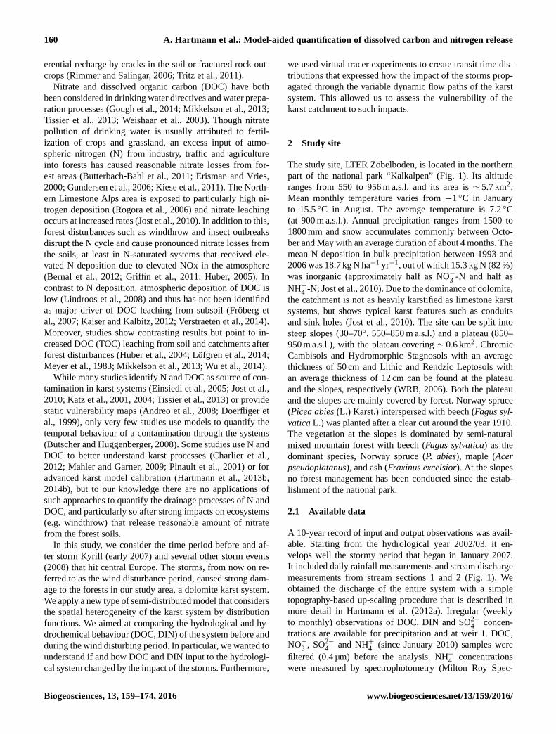
Figure 1. Study site and location of measurement devices (Hart-

mann et al., 2012a; modified).

tronic). Weekly DOC, SO2−4 and NO−3 samples were pooled

to provide volume weighted biweekly (until March 2009)

and monthly (thereafter) samples. DOC samples were acidi-

fied with 0.5 mL HCl 25 % and were measured with a Mai-

hak TOCOR 100 and a CPN TOC/DOC analyser (Shimadzu

Corp., Japan). NO−3 and SO2−4 concentrations were deter-

mined by ion chromatography with conductivity detection.

DIN input was then calculated as the sum of NO−3 -N and

NH+4 -N. Since NH+4 is either transformed into NO−3 or ab-

sorbed in the soil, NH+4 concentrations in runoff are very

small or not detectable. Therefore we calculated DIN out-

puts as NO−3 -N. Additionally, irregular observations of snow

water equivalent at the plateau allowed for independent setup

of the snow routines.

2.2 Recent disturbances

Kyrill in the year 2007 and some similarly strong storms sub-

sequent to 2008 caused some major windthrows as well as

single tree damages. A windthrow disturbance of ∼ 5 ha oc-

curred upstream of weir 1. Though no direct measurements

exist as to the total extent of the windthrow area we estimate

that 5–10 % of the study site has been subject to windthrow

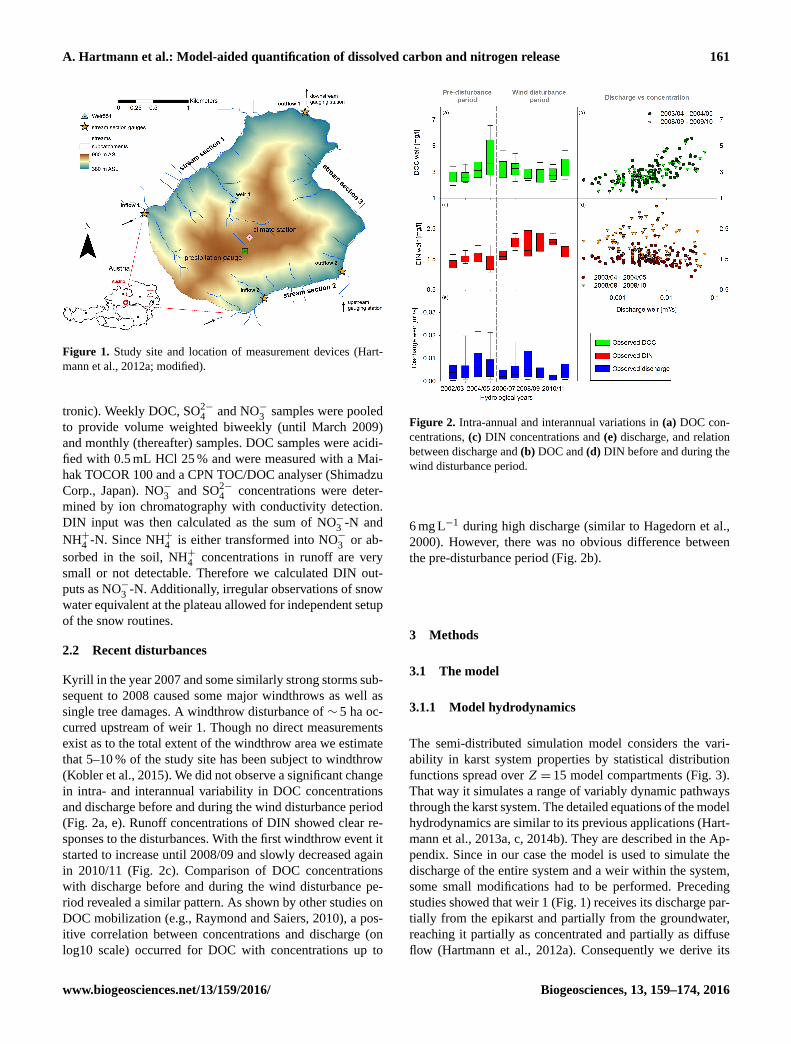
(Kobler et al., 2015). We did not observe a significant change

in intra- and interannual variability in DOC concentrations

and discharge before and during the wind disturbance period

(Fig. 2a, e). Runoff concentrations of DIN showed clear re-

sponses to the disturbances. With the first windthrow event it

started to increase until 2008/09 and slowly decreased again

in 2010/11 (Fig. 2c). Comparison of DOC concentrations

with discharge before and during the wind disturbance pe-

riod revealed a similar pattern. As shown by other studies on

DOC mobilization (e.g., Raymond and Saiers, 2010), a pos-

itive correlation between concentrations and discharge (on

log10 scale) occurred for DOC with concentrations up to

Figure 2. Intra-annual and interannual variations in (a) DOC con-

centrations, (c) DIN concentrations and (e) discharge, and relation

between discharge and (b) DOC and (d) DIN before and during the

wind disturbance period.

6 mg L−1 during high discharge (similar to Hagedorn et al.,

2000). However, there was no obvious difference between

the pre-disturbance period (Fig. 2b).

3 Methods

3.1 The model

3.1.1 Model hydrodynamics

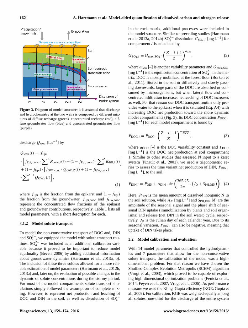
The semi-distributed simulation model considers the vari-

ability in karst system properties by statistical distribution

functions spread over Z = 15 model compartments (Fig. 3).

That way it simulates a range of variably dynamic pathways

through the karst system. The detailed equations of the model

hydrodynamics are similar to its previous applications (Hart-

mann et al., 2013a, c, 2014b). They are described in the Ap-

pendix. Since in our case the model is used to simulate the

discharge of the entire system and a weir within the system,

some small modifications had to be performed. Preceding

studies showed that weir 1 (Fig. 1) receives its discharge par-

tially from the epikarst and partially from the groundwater,

reaching it partially as concentrated and partially as diffuse

flow (Hartmann et al., 2012a). Consequently we derive its

www.biogeosciences.net/13/159/2016/ Biogeosciences, 13, 159–174, 2016

162 A. Hartmann et al.: Model-aided quantification of dissolved carbon and nitrogen release

Figure 3. Diagram of model structure; it is assumed that discharge

and hydrochemistry at the two weirs is composed by different mix-

tures of diffuse recharge (green), concentrated recharge (red), dif-

fuse groundwater flow (blue) and concentrated groundwater flow

(purple).

discharge Qweir [L s−1] by

Qweir(t)= fEpi

·

[fEpi, conc ·

∑Z

iRconc,i(t)+ (1− fEpi, conc) ·

∑Z

iRdiff,i(t)

]+ (1− fEpi) ·

[fGW, conc ·QGW,Z(t)+ (1− fGW, conc)

·

∑Z−1

iQGW,i(t)

],

(1)

where fEpi is the fraction from the epikarst and (1− fEpi)

the fraction from the groundwater. fEpi,conc and fGW,conc

represent the concentrated flow fractions of the epikarst

and groundwater contributions, respectively. Table 1 lists all

model parameters, with a short description for each.

3.1.2 Model solute transport

To model the non-conservative transport of DOC and, DIN

and SO2−4 , we equipped the model with solute transport rou-

tines. SO2−4 was included as an additional calibration vari-

able because it proved to be important to reduce model

equifinality (Beven, 2006) by adding additional information

about groundwater dynamics (Hartmann et al., 2013a, b).

The inclusion of these three solutes allowed for a more reli-

able estimation of model parameters (Hartmann et al., 2012b,

2013a) and, later on, the evaluation of possible changes in the

dynamic of solute concentrations during the stormy period.

For most of the model compartments solute transport sim-

ulations simply followed the assumption of complete mix-

ing. However, to represent net production and leaching of

DOC and DIN in the soil, as well as dissolution of SO2−4

in the rock matrix, additional processes were included in

the model structure. Similar to preceding studies (Hartmann

et al., 2013a, 2014b) SO2−4 dissolution GSO4,i [mg L−1] for

compartment i is calculated by

GSO4,i =Gmax,SO4·

(Z− i+ 1

Z

)aGeo

, (2)

where aGeo [–] is another variability parameter andGmax,SO4

[mg L−1] is the equilibrium concentration of SO2−4 in the ma-

trix. DOC is mostly mobilized at the forest floor (Borken et

al., 2011). Stored in the soil or diffusively and slowly pass-

ing downwards, large parts of the DOC are absorbed or con-

sumed by microorganisms, but when lateral flow and con-

centrated infiltration increase, net leaching of DOC increases

as well. For that reason our DOC transport routine only pro-

vides water to the epikarst when it is saturated (Eq. A4) with

increasing DOC net production toward the more dynamic

model compartments (Fig. 3). Its DOC concentration PDOC,i

[mg L−1] for each model compartment is found by

PDOC,i = PDOC ·

(Z− i+ 1

Z

)− 1aDOC

, (3)

where aDOC [–] is the DOC variability constant and PDOC

[mg L−1] is the DOC net production at soil compartment

1. Similar to other studies that assessed N input to a karst

system (Pinault et al., 2001), we used a trigonometric se-

ries to assess the time variant net production of DIN, PDIN,i

[mg L−1], to the soil:

PDIN,i = PDIN+ADIN · sin

(365.25

2π·(JD+ SPH,DIN

)). (4)

Here, PDIN is the mean amount of dissolved inorganic N in

the soil solution, while AN [mg L−1] and SPH,DIN [d] are the

amplitude of the seasonal signal and the phase shift of sea-

sonal DIN uptake (immobilization by plants and soil organ-

isms) and release (net DIN in the soil water) cycle, respec-

tively. JD is the Julian day of each calendar year. Due to its

seasonal variation, PDIN,i can also be negative, meaning that

uptake of DIN takes place.

3.2 Model calibration and evaluation

With 14 model parameter that controlled the hydrodynam-

ics and 7 parameters that allow for the non-conservative

solute transport, the calibration of the model was a high-

dimensional problem. For that reason we have chosen the

Shuffled Complex Evolution Metropolis (SCEM) algorithm

(Vrugt et al., 2003), which proved to be capable of explor-

ing high-dimensional optimization problems (Fenicia et al.,

2014; Feyen et al., 2007; Vrugt et al., 2006). As performance

measure we used the Kling–Gupta efficiency (KGE; Gupta et

al., 2009). For calibration, KGE was weighted equally among

all solutes, one-third for the discharge of the entire system

Biogeosciences, 13, 159–174, 2016 www.biogeosciences.net/13/159/2016/

A. Hartmann et al.: Model-aided quantification of dissolved carbon and nitrogen release 163

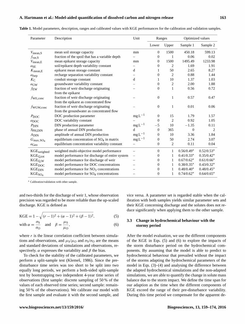
Table 1. Model parameters, description, ranges and calibrated values with KGE performances for the calibration and validation samples.

Parameter Description Unit Ranges Optimized values

Lower Upper Sample 1 Sample 2

Vmean,S mean soil storage capacity mm 0 1500 450.18 599.13

fvar,S fraction of the spoil that has a variable depth – 0 1 0.06 0.02

Vmean,E mean epikarst storage capacity mm 0 1500 1495.49 1233.98

aSE soil/epikarst depth variability constant – 0 2 1.69 1.91

Kmean,E epikarst mean storage constant d 1 50 2.65 8.27

afsep recharge separation variability constant – 0 2 0.88 1.44

KC conduit storage constant d 1 10 1.37 1.03

aGW groundwater variability constant – 0 2 2.00 1.88

fEW fraction of weir discharge originating – 0 1 0.56 0.72

from the epikarst

fWE,conc fraction of weir discharge originating – 0 1 0.57 0.47

from the epikarst as concentrated flow

fWGW,conc fraction of weir discharge originating – 0 1 0.01 0.06

from the groundwater as concentrated flow

PDOC DOC production parameter mg L−1 0 15 1.79 1.57

aDOC DOC variability constant – 0 2 0.92 1.05

PDIN DIN production parameter mg L−1−5 10 −1.35 0.11

SPH,DIN phase of annual DIN production d 0 365 0 2

ADIN amplitude of annual DIN production mg L−1 0 10 3.36 1.84

Gmax,SO4equilibrium concentration of SO4 in matrix mg L−1 0 50 2.74 3.07

aGeo equilibrium concentration variability constant – 0 2 0.11 0.04

KGEweighted weighted multi-objective model performance – 0 1 0.56/0.49∗ 0.52/0.53∗

KGEQ,tot model performance for discharge of entire system – 0 1 0.41/0.33∗ 0.35/0.42∗

KGEQ,W model performance for discharge of weir – 0 1 0.67/0.62∗ 0.61/0.66∗

KGEDOC model performance for DOC concentrations – 0 1 0.38/0.35∗ 0.43/0.32∗

KGEDIN model performance for NO3 concentrations – 0 1 0.48/0.40∗ 0.48/0.45∗

KGESO4model performance for SO4 concentrations – 0 1 0.74/0.62∗ 0.64/0.65∗

∗ Calibration/validation with other sample.

and two-thirds for the discharge of weir 1, whose observation

precision was regarded to be more reliable than the up-scaled

discharge. KGE is defined as

KGE= 1−

√(r − 1)2+ (α− 1)2+ (β − 1)2, (5)

with α =σS

σO

and β =µS

µO

, (6)

where r is the linear correlation coefficient between simula-

tions and observations, and µS/µO and σS/σO are the means

and standard deviations of simulations and observations, re-

spectively. α expresses the variability and β the bias.

To check for the stability of the calibrated parameters, we

perform a split-sample test (Klemeš, 1986). Since the pre-

disturbance time series was too short to be split into two

equally long periods, we perform a both-sided split-sample

test by bootstrapping two independent 4-year time series of

observations (first sample: discrete sampling of 50 % of the

values of each observed time series; second sample: remain-

ing 50 % of the observations). We calibrate our model with

the first sample and evaluate it with the second sample, and

vice versa. A parameter set is regarded stable when the cal-

ibration with both samples yields similar parameter sets and

their KGE concerning discharge and the solutes does not re-

duce significantly when applying them to the other sample.

3.3 Change in hydrochemical behaviour with the

stormy period

After the model evaluation, we use the different components

of the KGE in Eqs. (5) and (6) to explore the impacts of

the storm disturbance period on the hydrochemical com-

ponents. By assuming that the model is able to predict to

hydrochemical behaviour that prevailed without the impact

of the storms adapting the hydrochemical parameters of the

model in Eqs. (3)–(4) and analysing the difference between

the adapted hydrochemical simulations and the non-adapted

simulations, we are able to quantify the change in solute mass

balance due to the storm impact. We define the time span for

our adaption as the time when the different components of

KGE exceed the range of their pre-disturbance variability.

During this time period we compensate for the apparent de-

www.biogeosciences.net/13/159/2016/ Biogeosciences, 13, 159–174, 2016

164 A. Hartmann et al.: Model-aided quantification of dissolved carbon and nitrogen release

viations by adapting the hydrochemical parameters. This is

done twice – once by manual adaption and another time us-

ing an automatic calibration scheme. Their new values will

indicate changes in the seasonality, production or interannual

variations.

3.4 Transit time distributions

The signal of the storm impact will travel at various veloc-

ities and via pathways through the karst system. While fast

flow paths and small storages will transport the signal rapidly

to the system outlet, slow pathways and large storages will

delay and dilute the signal. Transit time distributions indi-

cate how fast surface impacts travel through the hydrological

system. We derive transit time distributions from the model

by performing a virtual tracer experiment with continuous

injection over the entire catchment at the beginning of the

impact of the stormy period. When a model compartment

reaches 50 % of the tracer concentration is considered me-

dian transit time. The thus-derived transit times will elaborate

how the hydrological system propagates the signal through

the system including all slow and fast pathways as defined

by Eqs. (12) and (18). As for DIN and DOC we assume

complete and instantaneous mixing with each model storage

(soil, epikarst, and groundwater) at each compartment; the

time that we refer to as “mean transit time” of a model com-

partment is the time the virtual tracer needs to pass through

the particular model storage. In combination with the fluxes

that are provided from each of the model compartments, it

is possible to quantify the fractional contribution of fast and

slow flow paths, respectively. We will apply the virtual tracer

from the previously assessed beginning of the impact un-

til the end of the time series to assess the transit time dis-

tribution. In addition, we apply a second virtual tracer that

also lasts only for the disturbance period (as estimated in

Sect. 3.3) to evaluate the filter and retardation potential of

the karst system.

4 Results

4.1 Model performance

Table 1 shows the calibrated parameters for the two samples.

They indicate a thick soil and a relatively thin epikarst. The

dynamics expressed by the storage constants indicate days

and weeks for the conduits (model compartment i = Z) and

the epikarst, respectively. The distribution coefficient of the

groundwater is larger than the soil/epikarst storage constant.

For DOC and DIN there are a natural production rates of 1.6–

1.8 and −1.35−0.1 mg L−1, respectively. The DOC distribu-

tion coefficient is between 0.9 and 1.1. The phase shift and

amplitude for DIN showed that there is a seasonal variation

in DIN net production, with its maximum release at April

each year for both of the samples. SO2−4 is dominated by the

concentration in the precipitation input with some leaching

in the soil and sulfides in the dolomite. Its variability con-

stant is quite low (< 0.1). Weighted KGEs, as well as their

values for the individual simulation variables, are relatively

stable. Overall, calibration on both samples provided similar

parameter values. Due to its higher stability concerning the

evaluation period, we chose the second sample for further

analysis.

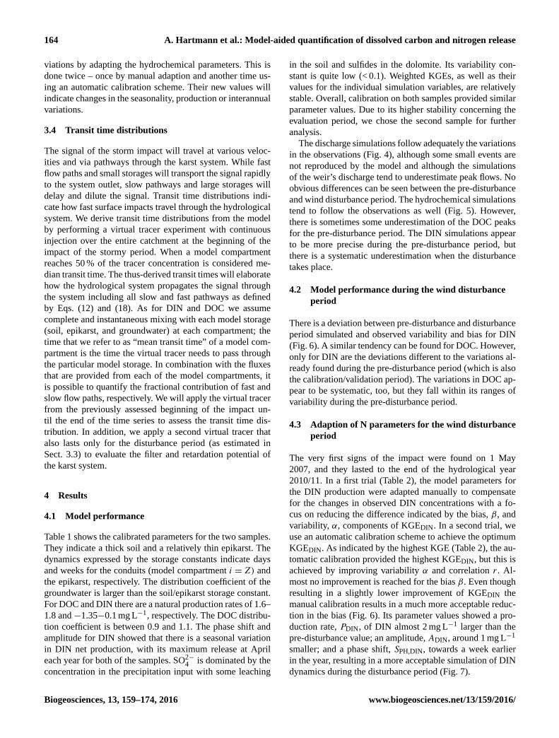
The discharge simulations follow adequately the variations

in the observations (Fig. 4), although some small events are

not reproduced by the model and although the simulations

of the weir’s discharge tend to underestimate peak flows. No

obvious differences can be seen between the pre-disturbance

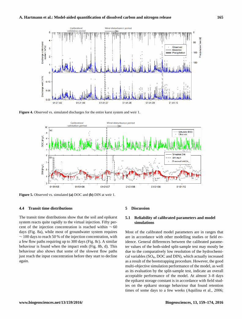
and wind disturbance period. The hydrochemical simulations

tend to follow the observations as well (Fig. 5). However,

there is sometimes some underestimation of the DOC peaks

for the pre-disturbance period. The DIN simulations appear

to be more precise during the pre-disturbance period, but

there is a systematic underestimation when the disturbance

takes place.

4.2 Model performance during the wind disturbance

period

There is a deviation between pre-disturbance and disturbance

period simulated and observed variability and bias for DIN

(Fig. 6). A similar tendency can be found for DOC. However,

only for DIN are the deviations different to the variations al-

ready found during the pre-disturbance period (which is also

the calibration/validation period). The variations in DOC ap-

pear to be systematic, too, but they fall within its ranges of

variability during the pre-disturbance period.

4.3 Adaption of N parameters for the wind disturbance

period

The very first signs of the impact were found on 1 May

2007, and they lasted to the end of the hydrological year

2010/11. In a first trial (Table 2), the model parameters for

the DIN production were adapted manually to compensate

for the changes in observed DIN concentrations with a fo-

cus on reducing the difference indicated by the bias, β, and

variability, α, components of KGEDIN. In a second trial, we

use an automatic calibration scheme to achieve the optimum

KGEDIN. As indicated by the highest KGE (Table 2), the au-

tomatic calibration provided the highest KGEDIN, but this is

achieved by improving variability α and correlation r . Al-

most no improvement is reached for the bias β. Even though

resulting in a slightly lower improvement of KGEDIN the

manual calibration results in a much more acceptable reduc-

tion in the bias (Fig. 6). Its parameter values showed a pro-

duction rate, PDIN, of DIN almost 2 mg L−1 larger than the

pre-disturbance value; an amplitude, ADIN, around 1 mg L−1

smaller; and a phase shift, SPH,DIN, towards a week earlier

in the year, resulting in a more acceptable simulation of DIN

dynamics during the disturbance period (Fig. 7).

Biogeosciences, 13, 159–174, 2016 www.biogeosciences.net/13/159/2016/

A. Hartmann et al.: Model-aided quantification of dissolved carbon and nitrogen release 165

Figure 4. Observed vs. simulated discharges for the entire karst system and weir 1.

Figure 5. Observed vs. simulated (a) DOC and (b) DIN at weir 1.

4.4 Transit time distributions

The transit time distributions show that the soil and epikarst

system reacts quite rapidly to the virtual injection. Fifty per-

cent of the injection concentration is reached within ∼ 60

days (Fig. 8a), while most of groundwater system requires

∼ 100 days to reach 50 % of the injection concentration, with

a few flow paths requiring up to 300 days (Fig. 8c). A similar

behaviour is found when the impact ends (Fig. 8b, d). This

behaviour also shows that some of the slowest flow paths

just reach the input concentration before they start to decline

again.

5 Discussion

5.1 Reliability of calibrated parameters and model

simulations

Most of the calibrated model parameters are in ranges that

are in accordance with other modelling studies or field ev-

idence. General differences between the calibrated parame-

ter values of the both-sided split-sample test may mostly be

due to the comparatively low resolution of the hydrochemi-

cal variables (SO4, DOC and DIN), which actually increased

as a result of the bootstrapping procedure. However, the good

multi-objective simulation performance of the model, as well

as its evaluation by the split-sample test, indicate an overall

acceptable performance of the model. At almost 3–8 days

the epikarst storage constant is in accordance with field stud-

ies on the epikarst storage behaviour that found retention

times of some days to a few weeks (Aquilina et al., 2006;

www.biogeosciences.net/13/159/2016/ Biogeosciences, 13, 159–174, 2016

166 A. Hartmann et al.: Model-aided quantification of dissolved carbon and nitrogen release

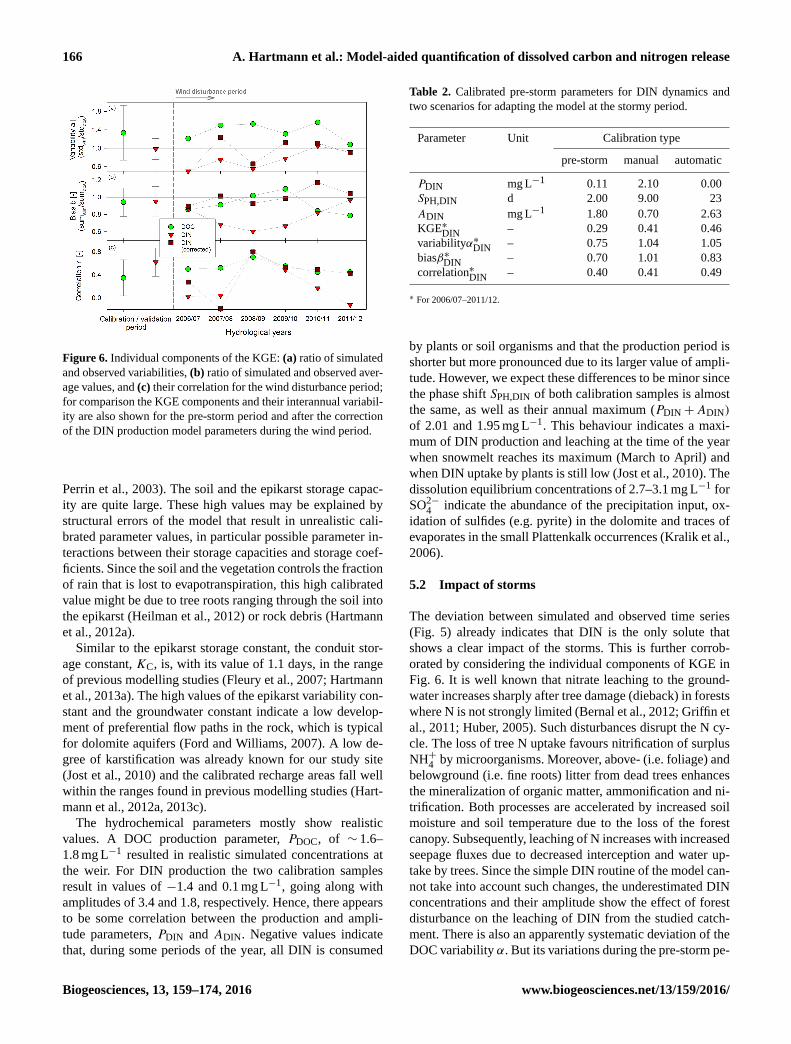
Figure 6. Individual components of the KGE: (a) ratio of simulated

and observed variabilities, (b) ratio of simulated and observed aver-

age values, and (c) their correlation for the wind disturbance period;

for comparison the KGE components and their interannual variabil-

ity are also shown for the pre-storm period and after the correction

of the DIN production model parameters during the wind period.

Perrin et al., 2003). The soil and the epikarst storage capac-

ity are quite large. These high values may be explained by

structural errors of the model that result in unrealistic cali-

brated parameter values, in particular possible parameter in-

teractions between their storage capacities and storage coef-

ficients. Since the soil and the vegetation controls the fraction

of rain that is lost to evapotranspiration, this high calibrated

value might be due to tree roots ranging through the soil into

the epikarst (Heilman et al., 2012) or rock debris (Hartmann

et al., 2012a).

Similar to the epikarst storage constant, the conduit stor-

age constant, KC, is, with its value of 1.1 days, in the range

of previous modelling studies (Fleury et al., 2007; Hartmann

et al., 2013a). The high values of the epikarst variability con-

stant and the groundwater constant indicate a low develop-

ment of preferential flow paths in the rock, which is typical

for dolomite aquifers (Ford and Williams, 2007). A low de-

gree of karstification was already known for our study site

(Jost et al., 2010) and the calibrated recharge areas fall well

within the ranges found in previous modelling studies (Hart-

mann et al., 2012a, 2013c).

The hydrochemical parameters mostly show realistic

values. A DOC production parameter, PDOC, of ∼ 1.6–

1.8 mg L−1 resulted in realistic simulated concentrations at

the weir. For DIN production the two calibration samples

result in values of −1.4 and 0.1 mg L−1, going along with

amplitudes of 3.4 and 1.8, respectively. Hence, there appears

to be some correlation between the production and ampli-

tude parameters, PDIN and ADIN. Negative values indicate

that, during some periods of the year, all DIN is consumed

Table 2. Calibrated pre-storm parameters for DIN dynamics and

two scenarios for adapting the model at the stormy period.

Parameter Unit Calibration type

pre-storm manual automatic

PDIN mg L−1 0.11 2.10 0.00

SPH,DIN d 2.00 9.00 23

ADIN mg L−1 1.80 0.70 2.63

KGE∗DIN – 0.29 0.41 0.46

variabilityα∗DIN – 0.75 1.04 1.05

biasβ∗DIN – 0.70 1.01 0.83

correlation∗DIN – 0.40 0.41 0.49

∗ For 2006/07–2011/12.

by plants or soil organisms and that the production period is

shorter but more pronounced due to its larger value of ampli-

tude. However, we expect these differences to be minor since

the phase shift SPH,DIN of both calibration samples is almost

the same, as well as their annual maximum (PDIN+ADIN)

of 2.01 and 1.95 mg L−1. This behaviour indicates a maxi-

mum of DIN production and leaching at the time of the year

when snowmelt reaches its maximum (March to April) and

when DIN uptake by plants is still low (Jost et al., 2010). The

dissolution equilibrium concentrations of 2.7–3.1 mg L−1 for

SO2−4 indicate the abundance of the precipitation input, ox-

idation of sulfides (e.g. pyrite) in the dolomite and traces of

evaporates in the small Plattenkalk occurrences (Kralik et al.,

2006).

5.2 Impact of storms

The deviation between simulated and observed time series

(Fig. 5) already indicates that DIN is the only solute that

shows a clear impact of the storms. This is further corrob-

orated by considering the individual components of KGE in

Fig. 6. It is well known that nitrate leaching to the ground-

water increases sharply after tree damage (dieback) in forests

where N is not strongly limited (Bernal et al., 2012; Griffin et

al., 2011; Huber, 2005). Such disturbances disrupt the N cy-

cle. The loss of tree N uptake favours nitrification of surplus

NH+4 by microorganisms. Moreover, above- (i.e. foliage) and

belowground (i.e. fine roots) litter from dead trees enhances

the mineralization of organic matter, ammonification and ni-

trification. Both processes are accelerated by increased soil

moisture and soil temperature due to the loss of the forest

canopy. Subsequently, leaching of N increases with increased

seepage fluxes due to decreased interception and water up-

take by trees. Since the simple DIN routine of the model can-

not take into account such changes, the underestimated DIN

concentrations and their amplitude show the effect of forest

disturbance on the leaching of DIN from the studied catch-

ment. There is also an apparently systematic deviation of the

DOC variability α. But its variations during the pre-storm pe-

Biogeosciences, 13, 159–174, 2016 www.biogeosciences.net/13/159/2016/

A. Hartmann et al.: Model-aided quantification of dissolved carbon and nitrogen release 167

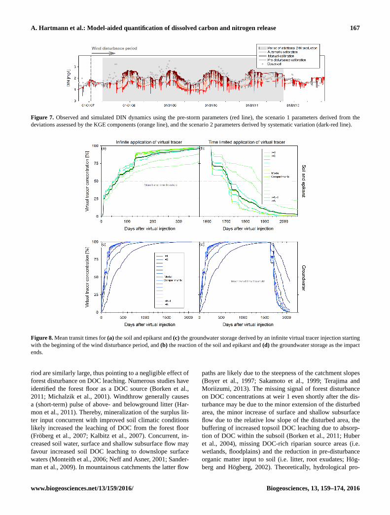
Figure 7. Observed and simulated DIN dynamics using the pre-storm parameters (red line), the scenario 1 parameters derived from the

deviations assessed by the KGE components (orange line), and the scenario 2 parameters derived by systematic variation (dark-red line).

Figure 8. Mean transit times for (a) the soil and epikarst and (c) the groundwater storage derived by an infinite virtual tracer injection starting

with the beginning of the wind disturbance period, and (b) the reaction of the soil and epikarst and (d) the groundwater storage as the impact

ends.

riod are similarly large, thus pointing to a negligible effect of

forest disturbance on DOC leaching. Numerous studies have

identified the forest floor as a DOC source (Borken et al.,

2011; Michalzik et al., 2001). Windthrow generally causes

a (short-term) pulse of above- and belowground litter (Har-

mon et al., 2011). Thereby, mineralization of the surplus lit-

ter input concurrent with improved soil climatic conditions

likely increased the leaching of DOC from the forest floor

(Fröberg et al., 2007; Kalbitz et al., 2007). Concurrent, in-

creased soil water, surface and shallow subsurface flow may

favour increased soil DOC leaching to downslope surface

waters (Monteith et al., 2006; Neff and Asner, 2001; Sander-

man et al., 2009). In mountainous catchments the latter flow

paths are likely due to the steepness of the catchment slopes

(Boyer et al., 1997; Sakamoto et al., 1999; Terajima and

Moriizumi, 2013). The missing signal of forest disturbance

on DOC concentrations at weir 1 even shortly after the dis-

turbance may be due to the minor extension of the disturbed

area, the minor increase of surface and shallow subsurface

flow due to the relative low slope of the disturbed area, the

buffering of increased topsoil DOC leaching due to absorp-

tion of DOC within the subsoil (Borken et al., 2011; Huber

et al., 2004), missing DOC-rich riparian source areas (i.e.

wetlands, floodplains) and the reduction in pre-disturbance

organic matter input to soil (i.e. litter, root exudates; Hög-

berg and Högberg, 2002). Theoretically, hydrological pro-

www.biogeosciences.net/13/159/2016/ Biogeosciences, 13, 159–174, 2016

168 A. Hartmann et al.: Model-aided quantification of dissolved carbon and nitrogen release

cesses such as a decrease in transpiration or an increase of

groundwater recharge may also occur. But these superficial

changes are probably minor considering the typically high

karstic infiltration capacities that remove surface water quite

rapidly (Hartmann et al., 2014b, 2015). Therefore, hydrolog-

ical impacts of windthrow on karst systems (for instance on

transpiration) may not be as pronounced as in non-karstic do-

mains because a large fraction of the infiltration during high

flow periods will not be available for transpiration anyway.

Consequently, a disturbance-caused impact on DOC avail-

ability could also be hidden because increased infiltration

and DOC leaching during strong rainfall events may just not

be detectable considering the weekly to monthly sampling

of DOC. For a better understanding of disturbance-induced

changes in DOC, more sampling in high temporal resolution

of DOC concentrations at the weir (Fig. 1) should be under-

taken to elucidate the effect of forest disturbance on DOC

dynamics and to improve the simulation of DOC production

and transport within the studied ecosystem

5.2.1 N leaching from the soil

Adapting the DIN solute transport parameters through use

of an automatic calibration scheme resulted in an increased

KGEDIN (Fig. 7). However, it did not resolve the bias of sim-

ulated and observed DIN concentrations during the wind dis-

turbance period since the overall improvement of KGEDIN

was reached by an improvement of r and α (Table 2). Ad-

justing the DIN parameters manually resulted in a more ac-

ceptable decrease in the bias β that also went along with

an increase of the overall KGEDIN. An increase of the DIN

production rate of ∼ 2 mg L−1 indicates a massive mobiliza-

tion of DIN and a reduction in its seasonal amplitude by

∼ 1.1 mg L−1. Even though there may be some correlation

between mean annual production and amplitude (see previ-

ous section), the annual maximum of 2.80 mg L−1 (PDIN+

ADIN) indicates an increase of the DIN concentrations in the

soil of at least∼ 0.8 mg L−1 (from 1.95 to 2.01 mg L−1 at the

pre-disturbance period).

We identified the beginning of the impact at 1 May 2007

and its end by the end of the hydrological year 2010/11.

This is more than 2 years after the last storm in 2008,

which indicates how long the ecosystem takes to recover

from the disturbance. Other studies have shown compara-

ble recovery times (Katzensteiner, 2003; Weis et al., 2006)

or longer (Huber, 2005). Considering the deviations between

DIN simulations by the pre-disturbance calibration and the

DIN simulations obtained by the manual adjustment, they

sum up to an additional release of 9.9 kg ha−1 of DIN over

the whole period of ∼ 3.7 years, or 2.7 kg ha−1 a−1 in addi-

tion to 5.8 kg ha−1 a−1 that would have been released without

the wind disturbance. These values only correspond to inor-

ganic N. Other studies showed that dissolved organic N can

also contribute to vertical percolation but only in small ra-

tios from 2 to 5 % (Solinger et al., 2001; Wu et al., 2009).

The apparent shift of SPH,DIN towards an earlier maximum

of DIN release (7 days) is most probably be due to the ear-

lier onset of snowmelt in open areas as compared to forests

because snowmelt is a major driver of DIN leaching from

the soils in our study area (Jost et al., 2010). However, due

to the rather slow melting rates, most of the melting water

will slowly/diffusively enter the groundwater system rather

than flowing rapidly through the karst conduits. Therefore, a

slightly earlier beginning of snowmelt may not be visible at

the system outlet due to the slow reaction of the groundwater

storage.

5.2.2 N propagation through the hydrological system

The virtual tracer injections that we applied with the begin-

ning of the disturbance period elaborate the hydrological sys-

tem’s filter and retardation capacity. Due to their higher dy-

namics, the soil and the epikarst system adapt more rapidly to

the change within weeks and months. Similar behaviour was

also found in previous studies (Hartmann et al., 2012a; Kralik

et al., 2009). The majority of the simulated flow paths adapt

to the virtual tracer signal within a few months, which is in

accordance with water isotope studies at the weir (Humer and

Kralik, 2008; Kralik et al., 2009). However, using age dating

(CFC and SF6) and artificial tracer experiments at individual

springs within the study area, Kralik et al. (2009) also found

ages from several days to several decades. Hence, the ma-

jority of transit times found by the virtual tracer experiment

reflect the average behaviour of the sub-catchment drained

by the weir, which can be regarded as more dominant than

observations at individual the springs that rather represent

fast and slow flow paths of minor importance. The retarda-

tion is also visible from the dynamics of the DIN concentra-

tions just after the end of the disturbance period (beginning of

2011/12, Fig. 7). Even though DIN production is set to pre-

disturbance conditions, it takes almost 4 months for the DIN

simulations (by manual calibration) to adapt to their undis-

turbed concentrations (pre-disturbance calibration). Due to

their small contribution (< 5 %), the slower flow paths do not

have a significant impact on the retardation capacity of the

hydrological system.

5.3 Implications

Our results corroborate findings from many other studies that

extreme events such as during the wind disturbance period

in our study can result in a significant increase in DIN in

the runoff, despite the area impacted being relatively small

(5–10 % of the watershed). Particularly in karst catchments,

such changes can happen quickly and prevail for a significant

duration, in our case more than 2 years after the last storm.

Due to subsurface heterogeneity, the impact did not travel

uniformly through the system. Instead, it split into different

pathways and mixed with old water that percolated prior to

the impact. In our system, large parts of the water travelled

Biogeosciences, 13, 159–174, 2016 www.biogeosciences.net/13/159/2016/

A. Hartmann et al.: Model-aided quantification of dissolved carbon and nitrogen release 169

rapidly through the system. However, a smaller number of

pathways had large storages of old water and slow flow ve-

locities, resulting in significant retardation. Taking into ac-

count that forest disturbances will most probably increase

with climate change (Seidl et al., 2014), DIN mobilization

as observed in our study may occur more often and become

more intense. The hydrological system may dilute and de-

lay rapid shifts of N concentration, and it will “memorize”

the impacts for some time. However, our present analysis

showed that the timescale of the wind disturbance on DIN

production and leaching from the soil exceeds the timescale

of transit of the disturbance through the system. This is most

probably due to the small size and the subsurface karstic

behaviour of our study site favouring faster flow paths and

lower system storage than hydrological systems with larger

extent or with other types of geology.

6 Conclusions

In our study we used a process-based semi-distributed karst

model to simulate DOC, DIN and SO2−4 transport through a

dolomite karst system in Austria. We calibrated and validated

our model during a 4-year time period just before a series of

heavy storms caused strong wind disturbance to the study

site’s ecosystem. To quantify its impact we ran the model for

the entire disturbance period using the parameters we found

at the pre-storm period. The deviations between the simula-

tions and the observations gave us an indication that there

was a significant shift in DIN mobilization, its seasonal am-

plitude and its timing. In estimating the beginning and end of

the disturbance period we applied a continuous virtual tracer

injection to obtain the mean transit times of the karst system.

The transit time distributions showed us how the hydrologi-

cal system filtered and retarded the impact of the disturbance

at the system outlet.

Even though our study is only considering one site and one

wind disturbance period, it provides some generally applica-

ble conclusions: (1) hydroclimatic extremes such as storms

not only create droughts or floods but can also affect water

quality; (2) a hydrological system can filter and delay surface

impacts, but it may also memorize past impacts, although

only at a limited timescale; and (3) water quality models that

have been calibrated without consideration of such external

impacts will provide poor predictions. For these reasons we

believe that future large-scale simulations of water resources

need to include water quality simulations that take into ac-

count the impact of ecosystem disturbances. Even without

anthropogenic contamination, climate change will strongly

affect water quality in our aquifers and streams, and we need

to understand processes that affect water quality and prepare

ourselves in order to avoid threats to future water supply.

www.biogeosciences.net/13/159/2016/ Biogeosciences, 13, 159–174, 2016

170 A. Hartmann et al.: Model-aided quantification of dissolved carbon and nitrogen release

Appendix A

The variability in soil depths in the model is expressed by

a mean soil depth, Vmean,S [mm], and a distribution coeffi-

cient, aSE [–]. The soil storage capacity, VS,i [mm], for every

compartment i is calculated by

VS,i =(1− fvar, S

)·Vmean, S+Vmax, S ·

(i

Z

)aSE

, (A1)

where the maximum soil storage capacity Vmax,S [mm] is de-

rived from (fvar,S × Vmean,S) as described in Hartmann et

al. (2013c). fvar,S [–] is the fraction of the soil that shows

variable thicknesses, while (1− fvar,S) has a uniform value.

The same distribution coefficient, aSE, is used to define the

epikarst storage distribution by the mean epikarst depth,

Vmean,E [mm] (derivation of Vmax,E identical to Vmean,S):

VE,i = Vmax,E ·

(i

Z

)aSE

. (A2)

Actual evapotranspiration from each soil compartment at

time step t , Eact,i , is found by

Eact,i(t)= Epot(t)

·min[VSoil,i(t)+P(t)+QSurface,i(t), VS,i]

VS,i

, (A3)

where Qsurface,i [mm d−1] is the surface inflow originating

from compartment i− 1 (see Eq. A7), Epot [mm d−1] the

potential evaporation, and P [mm d−1] the precipitation at

time t . Epot is calculated by the Penman–Wendling approach

(Wendling et al., 1991; DVWK, 1996). To account for the

solid fraction of precipitation, a snowmelt routine was set

at the top of the model. We used the same routine that

was applied to 148 other catchments in Austria by Para-

jka et al. (2007) and explained in Hartmann et al. (2012b).

Recharge to the epikarst, REpi,i [mm d−1], is defined as

REpi,i(t)=max[VSoil,i(t)+P(t)+QSurface,i(t)

−Eact,i(t)−VS,i,0], (A4)

where the storage coefficients KE,i [d] control the outflow of

the epikarst:

QEpi,i(t)=

min[VEpi,i(t)+REpi,i(t)+QSurface,i(t),VE,i]

KE,i

·1t (A5)

KE,i =Kmax, E ·

(Z− i+ 1

Z

)aSE

. (A6)

Kmax,E is derived by a mean epikarst storage coefficient,

Kmean,E (see Hartmann et al., 2013c). Excess water from the

soil and epikarst that produces surface flow to the next model

compartment, QSurf,i+1 [mm d−1], is calculated by

QSurf,i+1(t)=max[VEpi,i(t)+REpi,i(t)−VE,i,0]. (A7)

The lower outflow of each epikarst compartment is separated

into diffuse (Rdiff,i [mm d−1]) and concentrated groundwater

recharge (Rconc,i [mm d−1]) by the recharge separation fac-

tor, fC,i [–]:

Rconc,i(t)= fC,i ·QEpi,i(t), (A8)

Rdiff,i(t)= (1− fC,i) ·QEpi,i(t). (A9)

The distribution of fC,i among the different compartments is

defined by the distribution coefficient, afsep:

fC,i =

(i

Z

)afsep

. (A10)

Diffuse recharge reaches the groundwater compartment be-

low, while concentrated recharge is routed to the conduit

system (compartment i = Z). The variable contributions of

the groundwater compartments that represent diffuse flow

through the matrix (1. . .Z− 1) are given by

QGW,i(t)=VGW,i(t)+Rdiff,i(t)

KGW,i

. (A11)

KGW,i is calculated by

KGW,i =KC ·

(Z− i+ 1

Z

)−aGW

, (A12)

whereKC is the conduit storage coefficient. The groundwater

contribution of the conduit system originates from compart-

ment Z:

QGW,Z(t)=

min

[VGW,Z(t)+

Z∑i=1

Rconc,i(t),Vcrit, OF

]KC

.

(A13)

With the recharge area Amax [km2] known and the dimen-

sions [L s−1] rescaled, the discharge of the entire system Q

[L s−1] is calculated by

Q(t)=Amax

Z·

Z∑i=1

QGW,i(t). (A14)

Biogeosciences, 13, 159–174, 2016 www.biogeosciences.net/13/159/2016/

A. Hartmann et al.: Model-aided quantification of dissolved carbon and nitrogen release 171

Acknowledgements. Financial support is gratefully acknowledged

from the Transnational Access to Research Infrastructures activity

in the 7th Framework Programme of the EC as part of the ExpeER

project and the South East Europe Transnational Cooperation

Programme OrientGate for conducting the research. This work was

supported by a fellowship within the postdoc programme of the

German Academic Exchange Service (DAAD).

Edited by: M. Tzortziou

References

Andreo, B., Ravbar, N., and Vías, J. M.: Source vulnerability map-

ping in carbonate (karst) aquifers by extension of the COP

method: application to pilot sites, Hydrogeol. J., 17, 749–758,

doi:10.1007/s10040-008-0391-1, 2008.

Aquilina, L., Ladouche, B., and Doerfliger, N.: Water storage and

transfer in the epikarst of karstic systems during high flow peri-

ods, J. Hydrol., 327, 472–485, 2006.

Bakalowicz, M.: Karst groundwater: a challenge for new resources,

Hydrogeol. J., 13, 148–160, 2005.

Bernal, S., Hedin, L. O., Likens, G. E., Gerber, S., and Buso, D. C.:

Complex response of the forest nitrogen cycle to climate change,

109, 3406–411, doi:10.1073/pnas.1121448109, 2012.

Beven, K. J.: A manifesto for the equifinality thesis, J. Hydrol., 320,

18–36, 2006.

Borken, W., Ahrens, B., Schulz, C., and Zimmermann, L.: Site-to-

site variability and temporal trends of DOC concentrations and

fluxes in temperate forest soils, Glob. Chang. Biol., 17, 2428–

2443, doi:10.1111/j.1365-2486.2011.02390.x, 2011.

Boyer, E. W., Hornberger, G. M., Bencala, K. E., and McK-

night, D. M.: Response characteristics of DOC flushing

in an alpine catchment, Hydrol. Process., 11, 1635–1647,

doi:10.1002/(SICI)1099-1085(19971015)11:12< 1635::AID-

HYP494>3.0.CO;2-H, 1997.

Butscher, C. and Huggenberger, P.: Intrinsic vulnerability assess-

ment in karst areas: A numerical modeling approach, Water Re-

sour. Res., 44, W03408, doi:10.1029/2007WR006277, 2008.

Butterbach-Bahl, K., Gundersen, P., Ambus, P., Augustin, J., Beier,

C., Boeckx, P., Dannenmann, M., Sanchez Gimeno, B., Ibrom,

A., and Kiese, R.: Nitrogen processes in terrestrial ecosystems,

in The European nitrogen assessment: sources, effects and pol-

icy perspectives, edited by: Sutton, M. A., Howard, C. M., Eris-

man, J. W., Billen, G., Bleeker, A., Grennfelt, P., van Grisven,

H., and Grizzetti, B., Cambridge University Press, Cambridge,

United Kingdom and New York, NY, USA, 99–125, 2011.

Charlier, J.-B., Bertrand, C., and Mudry, J.: Conceptual hydroge-

ological model of flow and transport of dissolved organic car-

bon in a small Jura karst system, J. Hydrol., 460–461, 52–64,

doi:10.1016/j.jhydrol.2012.06.043, 2012.

Christensen, J. H., Hewitson, B., Busuioc, A., Chen, A., Gao,

X., Held, I., Jones, R., Kolli, R. K., Kwon, W.-T., Laprise, R.,

Rueda, V. M., Mearns, L., Menéndez, C. G., Räisänen, J., Rinke,

A., Sarr, A., and Whetton, P.: Regional Climate Projections, in

Climate Change 2007: The Physical Science Basis. Contribution

of Working Group I to the Fourth Assessment Report of the In-

tergovernmental Panel on Climate Change, edited by: Solomon,

S., Qin, D., Manning, M., Chen, Z., Marquis, M., Averyt, K.

B., Tignor, M., and Miller, H. L., Cambridge University Press,

Cambridge, United Kingdom and New York, NY, USA, 996

pp., available at: http://www.ipcc.ch/publications_and_data/

publications_ipcc_fourth_assessment_report_wg1_report_the_

physical_science_basis.htm (last access: 22 December 2015),

2007.

COST: COST 65: Hydrogeological aspects of groundwater protec-

tion in karstic areas, Final report (COST action 65), edited by:

Directorat-General XII Science, European Comission Research

and Development, Report EUR, 446 pp., 1995.

Dai, A.: Increasing drought under global warming in ob-

servations and models, Nature Climate Change, 3, 52–58,

doi:10.1038/nclimate1633, 2012.

Doerfliger, N., Jeannin, P.-Y., and Zwahlen, F.: Water vulnerabil-

ity assessment in karst environments: a new method of defining

protection areas using a multi-attribute approach and GIS tools

(EPIK method), Environ. Geol., 39, 165–176, 1999.

DVWK: Ermittlung der Verdunstung von Land- und Wasser-

flaechen (Estimating the evaporation of land and water surfaces),

Merkblaetter zur Wasserwirtschaft, Dtsch. Verband fuer Wasser-

wirtschaft und Kult. e.V., 238 pp., 1996.

Einsiedl, F., Maloszewski, P., and Stichler, W.: Estimation of

denitrification potential in a karst aquifer using the 15N

and 18O isotopes of NO3−, Biogeochemistry, 72, 67–86,

doi:10.1007/s10533-004-0375-8, 2005.

Erisman, J. W. and Vries, W. de: Nitrogen deposition and effects on

European forests, Environ. Rev., 8, 65–93, doi:10.1139/a00-006,

2000.

Fenicia, F., Kavetski, D., Savenije, H. H. G., Clark, M. P., Schoups,

G., Pfister, L., and Freer, J.: Catchment properties, function, and

conceptual model representation: is there a correspondence?, Hy-

drol. Process., 28, 2451–2467, doi:10.1002/hyp.9726, 2014.

Feyen, L., Vrugt, J. A., Nualláin, B. Ó., van der Knijff, J., and De

Roo, A.: Parameter optimisation and uncertainty assessment for

large-scale streamflow simulation with the LISFLOOD model,

J. Hydrol., 332, 276–289, doi:10.1016/j.jhydrol.2006.07.004,

2007.

Fleury, P., Plagnes, V., and Bakalowicz, M.: Modelling of the func-

tioning of karst aquifers with a reservoir model: Application to

Fontaine de Vaucluse (South of France), J. Hydrol., 345, 38–49,

2007.

Ford, D. C. and Williams, P. W.: Karst Hydrogeology and Geomor-

phology, Wiley, Chichester, 562 pp., 2007.

Fröberg, M., Jardine, P. M., Hanson, P. J., Swanston, C. W., Todd,

D. E., Tarver, J. R., and Garten, C. T.: Low Dissolved Organic

Carbon Input from Fresh Litter to Deep Mineral Soils, Soil Sci.

Soc. Am. J., 71, 347–354, doi:10.2136/sssaj2006.0188, 2007.

Goldscheider, N. and Drew, D.: Methods in Karst Hydrogeology,

edited by: International Association of Hydrogeologists, Taylor

& Francis Group, Leiden, NL, 264 pp., 2007.

Gough, R., Holliman, P. J., Heard, T. R., and Freeman, C.: Dis-

solved organic carbon and trihalomethane formation potential

removal during coagulation of a typical UK upland water with

alum, PAX-18 and PIX-322, J. Water Supply Res. Technol., 63,

650–660, 2014.

Griffin, J. M., Turner, M. G., and Simard, M.: Nitrogen cycling

following mountain pine beetle disturbance in lodgepole pine

forests of Greater Yellowstone, For. Ecol. Manage., 261, 1077–

1089, doi:10.1016/j.foreco.2010.12.031, 2011.

www.biogeosciences.net/13/159/2016/ Biogeosciences, 13, 159–174, 2016

172 A. Hartmann et al.: Model-aided quantification of dissolved carbon and nitrogen release

Gundersen, P., Schmidt, I. K., and Raulund-Rasmussen, K.: Leach-

ing of nitrate from temperate forests – effects of air pollution and

forest management, Environ. Rev., 14, 1–57, doi:10.1139/a05-

015, 2006.

Gupta, H. V, Kling, H., Yilmaz, K. K., and Martinez, G. F.: Decom-

position of the mean squared error and NSE performance criteria:

Implications for improving hydrological modelling, J. Hydrol.,

377, 80–91, doi:10.1016/j.jhydrol.2009.08.003, 2009.

Hagedorn, F., Schleppi, P., Waldner, P., and Flühler, H.: Export of

dissolved organic carbon and nitrogen from Gleysol dominated

catchments – the significance of water flow paths, Biogeochem-

istry, 50, 137–161, 2000.

Harmon, M. E., Bond-Lamberty, B., Tang, J., and Vargas, R.: Het-

erotrophic respiration in disturbed forests: A review with exam-

ples from North America, J. Geophys. Res.-Biogeosci., 116, 1–

17, doi:10.1029/2010JG001495, 2011.

Hartmann, A., Kralik, M., Humer, F., Lange, J., and Weiler, M.:

Identification of a karst system’s intrinsic hydrodynamic param-

eters: upscaling from single springs to the whole aquifer, Envi-

ron. Earth Sci., 65, 2377–2389, doi:10.1007/s12665-011-1033-9,

2012a.

Hartmann, A., Lange, J., Weiler, M., Arbel, Y., and Greenbaum, N.:

A new approach to model the spatial and temporal variability of

recharge to karst aquifers, Hydrol. Earth Syst. Sci., 16, 2219–

2231, doi:10.5194/hess-16-2219-2012, 2012b.

Hartmann, A., Barberá, J. A., Lange, J., Andreo, B., and Weiler,

M.: Progress in the hydrologic simulation of time variant

recharge areas of karst systems – Exemplified at a karst

spring in Southern Spain, Adv. Water Resour., 54, 149–160,

doi:10.1016/j.advwatres.2013.01.010, 2013a.

Hartmann, A., Wagener, T., Rimmer, A., Lange, J., Brielmann,

H. and Weiler, M.: Testing the realism of model struc-

tures to identify karst system processes using water quality

and quantity signatures, Water Resour. Res., 49, 3345–3358,

doi:10.1002/wrcr.20229, 2013b.

Hartmann, A., Weiler, M., Wagener, T., Lange, J., Kralik, M.,

Humer, F., Mizyed, N., Rimmer, A., Barberá, J. A., Andreo, B.,

Butscher, C., and Huggenberger, P.: Process-based karst mod-

elling to relate hydrodynamic and hydrochemical characteristics

to system properties, Hydrol. Earth Syst. Sci., 17, 3305–3321,

doi:10.5194/hess-17-3305-2013, 2013c.

Hartmann, A., Goldscheider, N., Wagener, T., Lange, J., and Weiler,

M.: Karst water resources in a changing world: Review of hy-

drological modeling approaches, Rev. Geophys., 52, 218–242,

doi:10.1002/2013rg000443, 2014a.

Hartmann, A., Mudarra, M., Andreo, B., Marín, A., Wagener,

T., and Lange, J.: Modeling spatiotemporal impacts of hy-

droclimatic extremes on groundwater recharge at a Mediter-

ranean karst aquifer, Water Resour. Res., 50, 6507–6521,

doi:10.1002/2014WR015685, 2014b.

Hartmann, A., Gleeson, T., Rosolem, R., Pianosi, F., Wada, Y.,

and Wagener, T.: A large-scale simulation model to assess

karstic groundwater recharge over Europe and the Mediter-

ranean, Geosci. Model Dev., 8, 1729–1746, doi:10.5194/gmd-8-

1729-2015, 2015.

Heilman, J. L., Litvak, M. E., McInnes, K. J., Kjelgaard, J.

F., Kamps, R. H., and Schwinning, S.: Water-storage capac-

ity controls energy partitioning and water use in karst ecosys-

tems on the Edwards Plateau, Texas, Ecohydrology, 7, 127–138,

doi:10.1002/eco.1327, 2012.

Hirabayashi, Y., Mahendran, R., Koirala, S., Konoshima, L., Ya-

mazaki, D., Watanabe, S., Kim, H., and Kanae, S.: Global flood

risk under climate change, Nature Climate Change, 3, 816–821,

doi::10.1038/nclimate1911, 2013.

Högberg, M. N. and Högberg, P.: Extramatrical ectomycorrhizal

mycelium contributes one-third of microbial biomass and pro-

duces, together with associated roots, half the dissolved or-

ganic carbon in a forest soil, New Phytol., 154, 791–795,

doi:10.1046/j.1469-8137.2002.00417.x, 2002.

Huber, C.: Long lasting nitrate leaching after bark beetle attack in

the highlands of the Bavarian Forest National Park., J. Environ.

Qual., 34, 1772–1779, doi:10.2134/jeq2004.0210, 2005.

Huber, C., Baumgarten, M., Göttlein, A., and Rotter, V.: Ni-

trogen turnover and nitrate leaching after bark beetle at-

tack in mountainous spruce stands of the Bavarian Forest

National Park, Water, Air, Soil Pollut. Focus, 4, 391–414,

doi:10.1023/B:WAFO.0000028367.69158.8d, 2004.

Humer, F. and Kralik, M.: Integrated Monitoring Zöbelboden: Hy-

drologische und hydrochemische Untersuchungen, Unpubl. Rep.

Environ. Agency, Vienna, 34 pp., 2008.

Johnson, M. S., Billett, M. F., Dinsmore, K. J., Wallin, M.,

Dyson, K. E., and Jassal, R. S.: Direct and continuous mea-

surement of dissolved carbondioxide in freshwater aquatic sys-

tems — method and applications, Ecohydrology, 159, 145–159,

doi:10.1002/eco.95, 2010.

Jost, G., Dirnböck, T., Grabner, M.-T., and Mirtl, M.: Nitrogen

Leaching of Two Forest Ecosystems in a Karst Watershed, Wa-

ter, Air, & amp, Soil Pollut., 218, 633–649, doi:10.1007/s11270-

010-0674-8, 2010.

Jourde, H., Mazzilli, N., Lecoq, N., Arfib, B., and Bertin, D.:

KARSTMOD: A Generic Modular Reservoir Model Dedicated

to Spring Discharge Modeling and Hydrodynamic Analysis in

Karst, in: Hydrogeological and Environmental Investigations in

Karst Systems SE – 38, vol. 1, edited by: Andreo, B., Carrasco,

F., J. Durán, J., Jiménez, P., and LaMoreaux, J. W., 339–344,

Springer Berlin Heidelberg., 2015.

Kaiser, K. and Kalbitz, K.: Cycling downwards – dissolved

organic matter in soils, Soil Biol. Biochem., 52, 29–32,

doi:10.1016/j.soilbio.2012.04.002, 2012.

Kalbitz, K., Meyer, A., Yang, R., and Gerstberger, P.: Response of

dissolved organic matter in the forest floor to long-term manipu-

lation of litter and throughfall inputs, Biogeochemistry, 86, 301–

318, doi:10.1007/s10533-007-9161-8, 2007.

Katz, B. G., Böhlke, J. K., and Hornsby, H. D.: Timescales for

nitrate contamination of spring waters, northern Florida, USA,

Chem. Geol., 179, 167–186, 2001.

Katz, B. G., Chelette, A. R., and Pratt, T. R.: Use of chemical

and isotopic tracers to assess nitrate contamination and ground-

water age, Woodville Karst Plain, USA, J. Hydrol., 289, 36–61,

doi:10.1016/j.jhydrol.2003.11.001, 2004.

Katzensteiner, K.: Effects of harvesting on nutrient leaching in a

Norway spruce (Picea), Plant Soil, 250, 59–73, 2003.

Kiese, R., Heinzeller, C., Werner, C., Wochele, S., Grote, R.,

and Butterbach-Bahl, K.: Quantification of nitrate leaching

from German forest ecosystems by use of a process ori-

ented biogeochemical model, Environ. Pollut., 159, 3204–14,

doi:10.1016/j.envpol.2011.05.004, 2011.

Biogeosciences, 13, 159–174, 2016 www.biogeosciences.net/13/159/2016/

A. Hartmann et al.: Model-aided quantification of dissolved carbon and nitrogen release 173

Klemeš, V.: Dilettantism in Hydrology: Transition or Destiny, Water

Resour. Res., 22, 177S–188S, 1986.

Kobler, J., Jandl, R., Dirnböck, T., Mirtl, M., and Schindlbacher,

A.: Effects of stand patchiness due to windthrow and bark beetle

abatement measures on soil CO2 efflux and net ecosystem pro-

ductivity of a managed temperate mountain forest, Eur. J. For.

Res., 13, 683–692, doi:10.1007/s10342-015-0882-2, 2015.

Kordilla, J., Sauter, M., Reimann, T., and Geyer, T.: Simulation

of saturated and unsaturated flow in karst systems at catchment

scale using a double continuum approach, Hydrol. Earth Syst.

Sci., 16, 3909–3923, doi:10.5194/hess-16-3909-2012, 2012.

Kralik, M., Humer, F., Grath, J., Numi-Legat, J., Hanus-Illnar, A.,

Halas, S., and Jelenc, M.: Impact of long distance air pollution

on sensitive karst groundwater resources estimated by means of

Pb-, S-, O- and Sr-isotopes, in: Karst, cambio climático y aguas

subterráneas, edited by: Duran, J. J., Andreo, B., and Carrasco,

F., Publicaciones del Instituto Geológico y Minero de España,

Serie: Hydrogeología y Aguas Subterráneas No 18, Madrid, 311–

317, 2006.

Kralik, M., Humer, F., Papesch, W., Tesch, R., Suckow, A., Han,

L. F., and Groening, M.: Karstwater-ages in an alpine dolomite

catchment, Austria: 18O , 3H , 3H/3He , CFC and dye tracer

investigations, Geophys. Res. Abstr., 11, 11403, European Geo-

sciences Union, General Assembly, 2009.

Le Moine, N., Andréassian, V., and Mathevet, T.: Confronting

surface- and groundwater balances on the La Rochefoucauld-

Touvre karstic system (Charente, France), Water Resour. Res.,

44, W03403, doi:10.1029/2007WR005984, 2008.

Lindroos, A. J., Derome, J., Mustajärvi, K., Nöjd, P., Beuker, E., and

Helmisaari, H. S.: Fluxes of dissolved organic carbon in stand

throughfall and percolation water in 12 boreal coniferous stands

on mineral soils in Finland, Boreal Environ. Res., 13, 22–34,

2008.

Löfgren, S., Fröberg, M., Yu, J., Nisell, J., and Ranneby, B.: Water

chemistry in 179 randomly selected Swedish headwater streams

related to forest production, clear-felling and climate, Environ.

Monit. Assess., 186, 8907–8928, doi:10.1007/s10661-014-4054-

5, 2014.

Mahler, B. J. and Garner, B. D.: Using Nitrate to Quantify

Quick Flow in a Karst Aquifer, Ground Water, 47, 350–360,

doi:10.1111/j.1745-6584.2008.00499.x, 2009.

Meyer, J. L., Tate, C. M., and Feb, N.: The Effects of Watershed Dis-

turbance on Dissolved Organic Carbon Dynamics of a Stream,

64, 33–44, 1983.

Michalzik, B., Kalbitz, K., Park, J., Solinger, S., and Matzner,

E.: Fluxes and concentrations of dissolved organic carbon and

nitrogen–a synthesis for temperate forests, Biogeochemistry, 52,

173–205, doi:10.1023/A:1006441620810, 2001.

Mikkelson, K. M., Bearup, L. A., Maxwell, R. M., Stednick, J. D.,

McCray, J. E., and Sharp, J. O.: Bark beetle infestation impacts

on nutrient cycling, water quality and interdependent hydrolog-

ical effects, Biogeochemistry, 115, 1–21, doi:10.1007/s10533-

013-9875-8, 2013.

Monteith, S. S., Buttle, J. M., Hazlett, P. W., Beall, F. D., Semkin,

R. G., and Jeffries, D. S.: Paired-basin comparison of hydro-

logic response in harvested and undisturbed hardwood forests

during snowmelt in central Ontario: II, Streamflow sources and

groundwater residence times, Hydrol. Process., 20, 1117–1136,

doi:10.1002/hyp.6073, 2006.

Neff, J. C. and Asner, G. P.: Dissolved organic carbon in terres-

trial ecosystems: Synthesis and a model, Ecosystems, 4, 29–48,

doi:10.1007/s100210000058, 2001.

Parajka, J., Merz, R., and Blöschl, G.: Uncertainty and multiple

objective calibration in regional water balance modelling: case

study in 320 Austrian catchments, Hydrol. Process., 21, 435–

446, doi:10.1002/hyp.6253, 2007.

Perrin, J., Jeannin, P.-Y., and Zwahlen, F.: Epikarst storage in a karst

aquifer: a conceptual model based on isotopic data, Milandre test

site, Switzerland, J. Hydrol., 279, 106–124, 2003.

Pinault, J.-L., Pauwels, H., and Cann, C.: Inverse modeling of the

hydrological and the hydrochemical behavior of hydrosystems:

Application to nitrate transport and denitrification, Water Resour.

Res., 37, 2179–2190, 2001.

Raymond, P. A. and Saiers, J. E.: Event controlled DOC ex-

port from forested watersheds, Biogeochemistry, 100, 197–209,

doi:10.1007/s10533-010-9416-7, 2010.

Rimmer, A. and Salingar, Y.: Modelling precipitation-streamflow

processes in karst basin: The case of the Jordan River sources,

Israel, J. Hydrol., 331, 524–542, 2006.

Rogora, M., Mosello, R., Arisci, S., Brizzio, M. C., Barbieri, A.,

Balestrini, R., Waldner, P., Schmitt, M., Stähli, M., Thimonier,

A., Kalina, M., Puxbaum, H., Nickus, U., Ulrich, E., and Probst,

A.: An Overview of Atmospheric Deposition Chemistry over the

Alps: Present Status and Long-term Trends, Hydrobiologia, 562,

17–40, doi:10.1007/s10750-005-1803-z, 2006.

Sakamoto, T., Takahashi, M., Terajima, T., Nakai, Y., and Mat-

suura, Y.: Comparison of the effects of rainfall and snowmelt

on the carbon discharge of a small, steep, forested watershed

in Hokkaido, northern Japan., Hydrol. Process., 13, 2301–2314,

doi:10.1016/j.rse.2007.01.011, 1999.

Sanderman, J., Lohse, K. A., Baldock, J. A., and Amundson, R.:

Linking soils and streams: Sources and chemistry of dissolved

organic matter in a small coastal watershed, Water Resour. Res.,

45, 1–13, doi:10.1029/2008WR006977, 2009.

Seidl, R., Schelhaas, M., Rammer, W., and Verkerk, P. J.: Increasing

forest disturbances in Europe and their impact on carbon stor-

age, Nature Climate Change, 4, 1–6, doi:10.1038/nclimate2318,

2014.

Solinger, S., Kalbitz, K., and Matzner, E.: Controls on the dynamics

of dissolved organic carbon and nitrogen in a Central European

deciduous forest, Biogeoch, 55, 327–349, 2001.

Terajima, T. and Moriizumi, M.: Temporal and spatial changes in

dissolved organic carbon concentration and fluorescence inten-

sity of fulvic acid like materials in mountainous headwater catch-

ments, J. Hydrol., 479, 1–12, doi:10.1016/j.jhydrol.2012.10.023,

2013.

Tissier, G., Perrette, Y., Dzikowski, M., Poulenard, J., Hobléa, F.,

Malet, E., and Fanget, B.: Seasonal changes of organic mat-

ter quality and quantity at the outlet of a forested karst system

(La Roche Saint Alban, French Alps), J. Hydrol., 482, 139–148,

doi:10.1016/j.jhydrol.2012.12.045, 2013.

Tritz, S., Guinot, V., and Jourde, H.: Modelling the be-

haviour of a karst system catchment using non-linear

hysteretic conceptual model, J. Hydrol., 397, 250–262,

doi:10.1016/j.jhydrol.2010.12.001, 2011.

Verstraeten, A., De Vos, B., Neirynck, J., Roskams, P., and

Hens, M.: Impact of air-borne or canopy-derived dis-

solved organic carbon (DOC) on forest soil solution DOC

www.biogeosciences.net/13/159/2016/ Biogeosciences, 13, 159–174, 2016

174 A. Hartmann et al.: Model-aided quantification of dissolved carbon and nitrogen release

in Flanders, Belgium, Atmos. Environ., 83, 155–165,

doi:10.1016/j.atmosenv.2013.10.058, 2014.

Vrugt, J. A., Gupta, H. V, Bouten, W., and Sorooshian, S.: A Shuf-

fled Complex Evolution Metropolis algorithm for optimization

and uncertainty assessment of hydrologic model parameters, Wa-

ter Resour. Res., 39, 1201, doi:10.1029/2002WR001642, 2003.

Vrugt, J. A., Gupta, H. V, Dekker, S. C., Sorooshian, S., Wagener,

T., and Bouten, W.: Application of stochastic parameter opti-

mization to the Sacramento Soil Moisture Accounting model,

J. Hydrol., 325, 288–307, doi:10.1016/j.jhydrol.2005.10.041,

2006.

Weis, W., Rotter, V., and Göttlein, A.: Water and element fluxes dur-

ing the regeneration of Norway spruce with European beech: Ef-

fects of shelterwood-cut and clear-cut, For. Ecol. Manage., 224,

304–317, doi:10.1016/j.foreco.2005.12.040, 2006.

Weishaar, J. L., Aiken, G. R., Bergamaschi, B. A., Fram, M. S.,

Fujii, R., and Mopper, K.: Evaluation of Specific Ultraviolet Ab-

sorbance as an Indicator of the Chemical Composition and Reac-

tivity of Dissolved Organic Carbon, Environ. Sci. Technol., 37,

4702–4708, doi:10.1021/es030360x, 2003.

Wendling, U., Schellin, H.-G., and Thomä, M.: Bereitstellung von

täglichen Informationen zum Wasserhaushalt des Bodens für die

Zwecke der agrarmeteorologischen Beratung – The supply of

daily information on the water budget of the soil as a contribu-

tion to the agrometeorological adviso, Zeitschrift für Meteorol.,

41, 468–475, 1991.

WRB: World reference base for soil resources, edited by: FAO,

IUSS Working Group, Rome, available at: http://www.fao.org/

ag/agl/agll/wrb/doc/wrb2006final.pdf (last access: 22 December

2015), 2006.

Wu, H., Peng, C., Moore, T. R., Hua, D., Li, C., Zhu, Q., Peichl, M.,

Arain, M. A., and Guo, Z.: Modeling dissolved organic carbon in

temperate forest soils: TRIPLEX-DOC model development and

validation, Geosci. Model Dev., 7, 867–881, doi:10.5194/gmd-7-

867-2014, 2014.

Wu, Y., Clarke, N., and Mulder, J.: Dissolved Organic Nitrogen

Concentrations and Ratios of Dissolved Organic Carbon to Dis-

solved Organic Nitrogen in Throughfall and Soil Waters in Nor-

way Spruce and Scots Pine Forest Stands Throughout Norway,

Water, Air, Soil Pollut., 210, 171–186, doi:10.1007/s11270-009-

0239-x, 2009.

Biogeosciences, 13, 159–174, 2016 www.biogeosciences.net/13/159/2016/