Habitat Selection by American Martens (Martes americana) in

Coastal Northwestern California

by

Keith M. Slauson

A THESIS

submitted to

Oregon State University

in partial fulfillment of the requirements for the

degree of

Master of Science

Presented April 25, 2003 Commencement June 2003

©Copyright by Keith M. Slauson April 25, 2003

All Rights Reserved

iii

AN ABSTRACT OF THE THESIS OF

Keith M. Slauson for the degree of Master of Science in Forest Science presented on April 25, 2003. Title: Habitat Selection by American Martens (Martes americana) in Coastal Northwestern California. Abstract approved: __________________________________________________

John P. Hayes The Humboldt marten, Martes americana humboldtensis, has undergone a dramatic

decline throughout its historical distribution in coastal Northwestern California. There

is currently only one known population occupying an area occurring in <5% of the

historical distribution of the subspecies. Conservation and management efforts to

benefit this population are hampered by lack of information on the habitat ecology of

martens in the coastal forest of northwestern California. Furthermore there have been

no investigations of the habitat ecology of marten populations anywhere in the coastal

forests of the Pacific States.

I investigated habitat relationships of the only known population of martens within

the historical distribution of M. a. humboldtensis at three spatial scales (microhabitat,

stand, and home range) and in relation to four forest management regimes (industrial

timberlands, and U. S. Forest Service (USFS) matrix lands, late-successional reserves,

and wilderness). Over 12 months of fieldwork during 2000 and 2001, I detected

iv

martens at 26 of 159 track plate sample units distributed on a systematic grid located

over the region known to be occupied by the population. I used an information-

theoretic approach to rank 56 a priori candidate models that described hypothesized

habitat relationships at each spatial scale.

Marten detections occurred in two distinct habitat types, those with forests on

serpentine soils and forests associated with more productive soil types, which are more

common in the region. At the microhabitat scale in serpentine habitats, martens were

detected at sites with dense shrub cover, sparse tree cover, and abundant surface rocks.

Dense shrub cover and abundant surface rocks may provide key overhead and escape

cover for martens in serpentine habitats. At the microhabitat scale in non-serpentine

habitats martens were detected at sites having the most mesic aspects, with dense tree

and shrub cover, and with a higher abundance of large diameter snags. At the stand

scale martens selected conifer-dominated stands with dense shrub cover in the latest

seral stages (old growth and late-mature) in non-serpentine habitats and variable seral

stages in serpentine habitats. At the home-range scale the probability of detecting a

marten decreased with increasing amounts of logging within 1-km of the sample unit

and increased with increasing maximum patch size of old growth, old growth plus

late-mature, or serpentine habitat within 1-km of the sample unit. Martens were

detected significantly more frequently in USFS lands than in private industrial

timberlands. Within USFS lands, martens were detected most frequently in matrix

and late-successional reserves, and least frequently in the wilderness area.

v

This study provides new information on the habitat ecology of martens in the

coastal forests of northwestern California. It demonstrates the importance of

investigating marten habitat at multiple spatial scales and provides insights to linkages

among scales and how martens respond to forest management. It also provides

information to aid conservation and restoration of martens in northwestern California

through identification of areas currently occupied or with suitable habitat, information

to identify suitable habitat in areas outside the study area, and information to guide

conservation planning for martens and site-specific habitat restoration.

vi

Master of Science thesis of Keith M. Slauson presented on April 25, 2003.

APPROVED:

________________________________________________________________ Major Professor, representing Forest Science ________________________________________________________________ Head of the Department of Forest Science ________________________________________________________________ Dean of the Graduate School

I understand that my thesis will become part of the permanent collection of Oregon State University libraries. My signature below authorizes release of my thesis to any reader upon request. _________________________________________________________________

Keith M. Slauson, Author

vii

ACKNOWLEDGEMENTS

Many individuals are deserving of recognition for their contributions to this project.

I must first thank Bill Zielinski for giving me the opportunity to challenge myself with

this project and for the guidance and friendship he provided throughout. Next I must

thank my major professor, John Hayes, for his support and guidance throughout the

design of the project and development of this thesis. I would also like to thank my

committee members John Tappeiner and Richard Schmitz for their insight and

suggestions during the development of the project and their thoughtful comments on

this thesis.

I want to especially thank and acknowledge the contributions and personal

sacrifices made by those who assisted me both as crew members and as friends in the

coastal mountains: Lisa Cross, Jessica Flayer, Jessie Grossman, Heather Lessig,

Julian Mangas, Giovanni Manghi, Ben Marckmann, Brit O’Brien, Jody Pennycook,

David Prins, Nick Polato, Jonothan Storm, Noel Soucy.

Many people made important contributions along the way. I must thank Quentin

Youngblood, Brenda Devlin, Kristin Schmidt, and especially Tony Hacking of the Six

Rivers National Forest for logistical and field support. Rick Schlexer, Chet Ogan, and

Rick Truex of the Redwood Sciences Lab provided important field and logistical

support. Jan Werren also of the Redwood Sciences Lab provided important GIS

support and training. Thomas Jimerson and Jeff Jones of the Ecology Program of the

Six Rivers National Forest provided important contributions and support in the use of

viii

the vegetation information for the study region. Lisa Gaino and Manuela Huso of the

Department of Forest Science provided important statistical advice and support.

I wish to thank the Simpson Timber Company and Keith Hamm, Lowell Diller, and

Chris Howard for assisting us with access and logistics on company lands.

And finally I must acknowledge the individuals and organizations who helped to

provide the financial support: Esther Burkett, California Department of Fish and

Game; Department of Forest Science, Oregon State University; Ruskin Hartley, Save-

The-Redwoods League; Redwood Sciences Lab, U.S.D.A. Forest Service-Pacific

Southwest Research Station; Six Rivers National Forest, U.S.D.A. Forest Service;

Amedee Brickey, Arcata Office of the U.S.D.I. Fish and Wildlife Service.

And of course I need to acknowledge the lean beasts who left little more than paw

prints as evidence of their presence, but from which we’ve begun to understand a bit

of their fascinating ecology in the coastal forests of California.

ix

TABLE OF CONTENTS

Page

INTRODUCTION.......................................................................……………………..1 METHODS..............................................................................………………………10 Study Area………………………………………………………………........10 Detection Methods…………………...……………………………………… 13 Sampling Design…………………..………………………………… 13 Track Plates.......................................................................................... 13 Live Trapping………………………..………………………………. 15 Multi-scale Habitat Classification and Sampling………………………......... 15

Microhabitat Scale…………………………………………………... 15 Stand and Home Range scales………………………………………. 18 Stand Scale…………………………………………………... 19

Home Range Scale……………………………………..……. 22 Mixed Scale…………………………………………………. 24 Management Units…………………………………………………... 24

Statistical Analysis…………………………………………………………... 26

Microhabitat Analysis……………………………………………...... 26 Stand, Home Range, and Mixed Scale Analysis…………………...... 26 Management Unit Comparison.……………………………………... 31 RESULTS………………………………………...…………………………………. 33 Sample Unit Results……………………………………………...………….. 33 Live Trapping Results.……………………………………………...……….. 33 Multi-scale Habitat Analysis………………………………………..……….. 35

Microhabitat Scale…………………………………………………... 36 Stand Scale…………………………………………………………... 44

Home Range Scale…………………………………………………... 49 Mixed Scale……………………………………...……………….….. 54 Management Unit Comparison……………………………………….……... 58

x

TABLE OF CONTENTS (Continued)

Page DISCUSSION……………………………………………………………………….. 60 Multi-scale Habitat Characteristics………………………………………….. 60 Microhabitat Characteristics…………………………………….…... 61 Stand Scale Habitat Selection……………………………………….. 63 Home Range Scale Habitat Selection……………………….………. 67 Management Units…………………………………………………………... 69 Conservation and Management Implications………….….............................. 70 Scope of Inference………………………………………………….……….. 73 Research Needs……………………………………………………………… 75 LITERATURE CITED……………………………………...………………………. 78 APPENDICES………………………………………………………………….…… 88

xi

LIST OF FIGURES

Figure Page 1. Study area, ownership, preexisting marten detections and new sampling grid..………...................................................................................... 11 2. Composition of old growth, serpentine and percent logged area for each management unit……………………………………………………..…..….. 25 3. Relative vegetation series composition for each management unit……......... 26 4. Sample units completed and marten detections within the study grid….…… 34

5. Marten detection results and the distribution of serpentine and non-serpentine habitats……………………..………...……………..………. 35

6. Proportions of stations in 8 macro-aspect categories for all used and unused stations..…………………………………….……………………….. 37 7. Use and availability of seral stages for non-serpentine stands where martens were and were not detected………….............................................................. 48 8. Use and availability of seral stages for serpentine stands where martens

were and were not detected………….............................................................. 48 9. Classification success for the best stand scale model………….…..…........... 49 10. The relative proportion by size classes for the maximum contiguous old growth, old growth plus late mature, or serpentine patch within a 1-km radius for each sample unit………………..………...……..………... 53 11. Classification success for the best home range scale model………...………. 54 12. Classification success for the best mixed scale model……..…...…………… 57 13. Marten detection results and management units……………...……..………. 59

xii

LIST OF TABLES

Table Page 1. Description of the habitat variables measured at the microhabitat scale...….. 16 2. Description of the habitat variables measured at the stand scale….……….... 19 3. Description of the habitat variables measured within 1-km radius circles around each grid point…………………………..………………….... 23 4. Variable screening criteria………………..………..………………………... 29 5. Micro-slope position for each track plate station…………...………….......... 36 6. Macro-aspect for each track plate station…...……………………….……..... 37 7. Canopy closure characteristics for all used and unused stations……….…..... 38

8. Declining rank-order tree species dominance for 0.49 Ha plots where martens were detected……………………………………………….….…… 39 9. Basal area (m2 / ha) estimated using a 20-factor prism, with each track plate station as plot center……………………………………………............ 40 10. Number of snags included in the 20-factor prism sample and their mean diameters at breast height (dbh)……………………………..…..…..... 41 11. Rank-order shrub species dominance for 0.49 Ha plots where martens were detected………………………………………………………………… 42 12. Mean percent ground cover values for microhabitat (0.49 ha) plots centered on track plate stations…………………………...…………….…… 43 13. Summary of variables characterizing sites where martens were detected at the microhabitat scale. All variables listed represent those with large differences between sites where martens were and were not detected………………………………………………………………............ 44 14. Resource selection probability function (RSPF) results for the stand scale………………………………………………………………………….. 45 15. Normalized importance weights for stand scale variables……...……...……. 46

xiii

LIST OF TABLES (Continued)

Table Page 16. Variable coefficients and odds ratios for the best stand model (Model 1, Table 14)…………………………………………………………. 47 17. Resource selection probability function (RSPF) results for the home-range scale……………………………………………………….......... 50 18. wi corrected for model redundancy for the 95% confidence set of home-range scale models…………………………………………………… 51 19. Normalized importance weights for all home-range scale variables….…….. 52 20. Resource selection probability function (RSPF) results for the mixed scale……………………………………………………………........... 55 21. Normalized importance weights for all mixed scale variables……..…...…... 56 22. Variable coefficients and odds ratios for the best mixed scale RSPF.............. 56

xiv

LIST OF APPENDICES

Appendix Page A. Animal handling and immobilization procedure……………..……………... 89 B. List and descriptions for all GIS coverages used……………...…………….. 93 C. Selected descriptive variables, log and snag data for seral stages in the Tanoak and Douglas-fir vegetation series……………………………….…... 94 D. CWHR classification results for micro-habitat sites……………...…………. 97 E. SAS Code for AIC Calculation, ∆AIC…………...…………………………. 99 F. Univariate results for all stand and home range scale variables.................... 107 G. Results and characteristics of vegetation series and subseries where martens were detected………………………………………………..…….. 109

xv

LIST OF APPENDIX TABLES

Table Page D-1 CWHR results for all stations where martens were detected .……………… 98 F-1 Univariate descriptive statistics for stand scale variables………...………... 107 F-2 Univariate descriptive statistics for home-range scale

variables…………………………………………………………….……… 108

xvi

LIST OF APPENDIX FIGURES

Figure Page

G-1 Percent used and available for the five most frequently sampled vegetation series…………………………...………………………...…………………. 111 G-2 Seral stage distribution by vegetation series for all 159 sampled stands………………..……………………………………..……………….. 112

1

Habitat Selection by American Martens (Martes americana) in Coastal

Northwestern California

INTRODUCTION

The American marten (Martes americana) is composed of 14 recognized

subspecies and is broadly distributed throughout boreal and coastal coniferous forests

in North America (Hall 1981). In the western United States the distribution is highly

peninsularized, tracking the distribution of coniferous forests on interior (e.g., Rocky

Mountains, Cascades, and Sierra Nevadas) and coastal (e.g., Olympic Peninsula, and

Oregon and California coast ranges) mountain ranges. The contemporary distribution

of American martens has declined from that of pre-settlement period of European

peoples (Giblisco 1994) and the most dramatic declines have occurred in the maritime

regions of both the Atlantic and Pacific coasts (Bergerud 1969, Dodds and Martell

1971, Giblisco 1994, Zielinski and Golightly 1996, Zielinski et al. 2001). Of the 14

subspecies of American martens recognized by Hall (1981), M. a. atrata on the island

of Newfoundland has received the most conservation attention and has been

designated a red list species by the Canadian Fish and Wildlife Service. Recently,

Zielinski et al. (2001) documented a substantial decline in the distribution of another

recognized subspecies, the Humboldt marten, (M. a. humboldtensis, Grinnell and

Dixon 1926). The Humboldt marten is endemic to the coastal forests of northwestern

California and was originally described as occurring in “the narrow northwest humid

coast strip, chiefly within the redwood belt” from the Oregon border to northern

Sonoma county (Grinnell et al. 1937). In the early 1900s the Humboldt marten was

2

already declining due to intense trapping pressure (Grinnell et al. 1937). Despite

closure of the trapping season for martens in California in the late 1940s, populations

of the Humboldt marten apparently have never recovered. During the same period

that efforts were taken to conserve the remaining martens through the cessation of

trapping for their fur, the region’s primary forests were logged at an accelerating rate

(Bolsinger and Waddell 1993). During the 1900’s, roughly 95% of the redwood

forests were converted from mature and old-growth stands to structurally and

compositionally different stands of 80 years or less (Thornburg et al. 2000). Adjacent

near-coast coniferous forest types, such as those dominated by Douglas-fir, have

undergone a similar pattern of loss of mature and old- growth stands (Bolsinger and

Waddell 1993).

Currently there is only one known population of martens that occupies less than 5%

of the historical range of the Humboldt subspecies (Zielinski et al. 2001, Slauson et al.

2002). Conservation efforts or management alternatives favoring marten populations

are hampered by a lack of information on their habitat ecology and their response to

forest management in the coastal forests of California. There have been no

investigations of the habitat ecology of the Humboldt marten or within coastal forest

habitats occupied by M. a. caurina in Oregon or Washington. The only published

studies on the habitat ecology of martens in Pacific coastal forests were conducted by

Baker (1992) on Vancouver Island, British Columbia and Schumacher (1999) in

southeast Alaska.

3

Habitat selection occurs hierarchically at each of the scales to which a species

responds. Individual animals respond to their environment over several spatial scales,

with the smallest scale corresponding to the grain of the animal, and the largest scale

being at least its home range (Kotliar and Wiens 1990). Different aspects of an

animal’s life history (e.g., daily resting, winter foraging, finding mates) motivate

selection at each of these scales (Bissonette et al. 1997). Investigations of habitat

selection must carefully determine which habitat characteristics are important to

consider and at what spatial scale they should be measured (Johnson 1980). Multi-

scale investigations are generally superior to single-scale investigations because

studies conducted over several spatial scales facilitate a greater understanding of how

animals assimilate information and make decisions that influence habitat selection

(Ritchie 1997). To reach valid conclusions in studies of habitat selection, used habitat

characteristics should be compared to available or unused habitat characteristics

(Manly et al. 1993). When habitat characteristics are used disproportionate to their

availability, use is said to be selective (Manly et al. 1993). The development of an

understanding for the characteristics of forest habitats selected by martens at multiple

spatial scales in coastal northwestern California can provide a strong foundation from

which conservation and management alternatives favoring martens can be developed.

The American marten is considered one of the most habitat-specific mammals

in North America (Harris 1984, Buskirk and Ruggiero 1994). Throughout most

of their distribution martens are associated with closed-canopy, late-successional

stands of mesic conifers with complex structure on or near the ground (Buskirk

4

and Ruggiero 1994, Buskirk and Powell 1994). Martens avoid open areas lacking

overhead cover or vertical tree boles that provide vertical escape routes from predators

(Drew 1995).

Martens are highly mobile animals and have home ranges that are 3-4 times larger

than predicted for a 1 kg terrestrial mammalian carnivore (Buskirk and Ruggiero

1994). Bissonette et al. (1997) demonstrated that martens select habitat at three spatial

scales and that a fourth scale operates as an upper-level constraint to habitat selection.

These include the micro or sub-stand (several square meters), stand (several hectares),

home range (one half to several square kilometers), and landscape scales (tens to

hundreds of square kilometers).

At the microhabitat scale, martens select specific habitat features that provide

foraging, resting, and denning opportunities. Martens likely choose foraging locations

where prey species are abundant and where the habitat structure at the site renders

prey vulnerable to capture (Buskirk and Powell 1994). Martens are considered dietary

generalists, but show strong seasonal variation with respect to the types of food items

taken (Strickland and Douglas 1987, Martin 1994). Martens take advantage of

seasonally abundant foods, such as fruits and insects during the summer and fall

(Koehler and Hornocker 1977, Simon 1980). Several mammal species including,

voles (Clethrionomys, Microtus), pine squirrels (Tamaisciurus.), ground squirrels

(Spermophilus), and chipmunks (Tamias) are important components of the diet of

martens in the western United States (Martin 1994). Voles and pine squirrels are most

important during the winter months when prey options are most limited (Buskirk and

5

Ruggiero 1994), and ground squirrels and chipmunks become important during the

summer months (Zielinski et al. 1983). This seasonal variation in diet likely results in

seasonal variation in the selection of microhabitat for foraging to match that of the

prey species.

Martens use rest sites between periods of activity and females use natal dens to

give birth to their kits in the spring and later move them to one or more maternal dens

until they are old enough to disperse on their own. Martens select structures for

resting and denning that will provide both thermal refugia (Taylor 1993) and refugia

from predators. Seasonal variation in use of rest structure types occurs, with above-

ground structures used more during summer and fall and below-ground or subnivien

structures used more during winter (Wilbert 1992, Gilbert et al. 1997, Raphael and

Jones 1997, Chapin et al. 1998). Rest structures typically include cavities or platforms

in live trees or snags, cavities in logs, and, to a lesser extent, rock piles, slash piles,

and subterranean cavities (e.g., those created by rotting root wads) (Raphael and Jones

1997, Gilbert et al. 1997, Ruggiero et al. 1998, Bull and Heater 2000). Den structures

typically include arboreal cavities in live trees, snags (Gilbert et al. 1997, Raphael and

Jones 1997, Bull and Heater 2000) and logs, rock crevices and red squirrel middens

(Ruggiero et al. 1998). Resting and denning sites are most commonly located in

woody structures (live trees, snags, logs) that tend to be in the largest available size

classes and are used disproportionate to their availability (Wilbert 1992, Gilbert et al.

1997, Raphael and Jones 1997, Ruggiero et al. 1998).

6

At the stand scale, martens select stands with the structural features that provide for

one or more life-history requirements (e.g., prey populations, resting structures). Most

studies have found that martens use mid- or late-successional stands of mesic conifers

with complex physical structure near the ground and dense canopy closure (Buskirk

and Powell 1994). Clear-cut and heavily logged stands generally are not used for

several decades following logging, however this varies by location, and is most likely

dependent on the time to development of a closed canopy and structural complexity

near and on the ground return to the stand (Buskirk and Powell 1994). Two key prey

species in the winter diet of martens in the western U.S., red-backed voles

(Clethrionomys californicus and C. gapperi) and Douglas squirrels (Tamaisciurus

douglasii), are closely associated with elements of late successional forest structure.

Both are more abundant in mature coniferous forests, with the former being most

closely associated with abundant large diameter downed woody debris and logs

(Hayes and Cross 1987, Raphael 1989, Tallmon and Mills 1994) and the latter with

cone-producing stages, especially in late-successional stages (Flyger and Gates 1982).

Moreover, several studies have found that there are seasonal differences in the ages of

stands used by martens, with a selection for older forests during the winter (Buskirk

and Ruggiero 1994).

Martens forage over portions of their home ranges sequentially, resting in trees and

snags in close proximity to the locations of their foraging areas and most recent kill

sites (Marshall 1946, Spencer 1981). Low rates (< 25%) of re-use of rest sites indicate

that numerous suitable resting structures need to be available within each individual

7

marten’s home range (Raphael and Jones 1997, Zielinski et al. 1996). This, combined

with seasonal shift in the use of above- and below-ground resting structures, indicates

the need for stands included in marten home ranges to contain multiple suitable resting

structures within each structure type (e.g., snags, logs). In western forests, large live

trees, snags, and downed logs are most abundant in stands that are in late successional

stages.

At the home-range scale, martens position their home ranges to include forest

stands that provide for year round life history needs (e.g., seasonal prey bases, access

to mates) while avoiding same-sex conspecifics (Katnik et al. 1994). Home range size

has been shown to vary depending on prey abundance and habitat type (Soutiere 1979,

Thompson and Colgan 1987). Mean home range estimated from reviewed nine

studies ranged from 0.8 km2 to 15.7 km2 for male martens whereas female martens

used home ranges that averaged about one-half that size (Buskirk and McDonald

1989). Home ranges in landscapes with clearcuts can be from 1.5 to 3.1 times greater

than those from landscapes without clearcuts (Thompson and Colgan 1987). Katnik

(1992) found that in an industrial forest site, martens occupied home ranges that

included more mature forest and less clearcut and regenerating forest relative to their

availability. In an adjacent forest reserve, where clearcuts and regenerating forest

were not present, martens did not exhibit selection at the home-range scale (Chapin et

al. 1998). Martens appear to consider habitat heterogeneity, interspersion, and

juxtaposition when establishing a home range, but at some threshold suitable habitat

8

becomes too dispersed to be adequate for an individual to maintain a home range that

meets its energetic and ecological needs (Bissonette et al. 1997).

At the landscape scale, dispersing individuals select from suitable portions of the

landscape unoccupied by same-sex conspecifics to establish home ranges. Loss and

fragmentation of mature forest and the resulting changes in landscape pattern constrain

animal movement (Bissonette et al.1989, Chapin 1995, Hargis 1996) and demography

(Fredrickson 1990, Hargis 1996). Studies conducted in Maine, Utah, and Quebec

found that martens appear to avoid landscapes with more than 25-30% of mature

forest removed (Bissonette et al. 1997, Potvin et al. 2000). Landscape characteristics,

such as distance between small and large patches have been shown to influence the

use of patches by martens (Chapin et al. 1998). Phillips (1994) demonstrated that

martens used only 33% of the available landscape in the industrial forest site, while

they occupied >80% of the landscape in a nearby forest preserve. Marten responses to

landscape-level changes in forest area and configuration of mature forest patches have

not been previously studied in coastal forests of the Pacific states, despite the fact that

most of these forests are currently intensively managed for timber production, with

much of the landscape already exceeding the 25-30% mature forest-loss threshold

(United States Department of Agriculture 1992, Bolsinger and Waddell 1993,

Thornburg et al. 2000).

The purpose of this study is to investigate habitat selection at multiple spatial scales

by the only known population of American martens within the historical range of M.

a. humboldtensis. The objectives of this study are to determine: 1) the microhabitat

9

characteristics at sites used by Humboldt martens, 2) the characteristics of the habitat

selected by martens at the stand and home-range scales, and 3) whether the number or

proportion of marten detections vary by forest management regime. This study will

provide important new information on the habitat ecology of martens within the

historical range of the Humboldt subspecies and is the first study of the habitat

ecology of martens in the coastal forests of the Pacific states. This information will be

important for developing conservation, restoration, and management options that will

favor martens in coastal northwestern California.

10

METHODS

Study Area

My study area is approximately 800 km2 (300 mi2) and is located in coastal

northwestern California (123° 45’ 00’’, 41° 30’ 00’’). It includes portions of

southern Del Norte, northern Humboldt, and western Siskiyou counties.

The majority (78.3%) falls within the Smith River National Recreation Area

(SMNRA) and the Orleans Ranger District (ORD) of the Six Rivers National Forest

and the Ukonom Ranger District (URD) of the Klamath National Forest. The

remainder of the study area is within lands owned and managed by the Simpson

Timber Company (STC) (Figure 1). There are 4 different management units within

the study area: Siskiyou Wilderness (18.2%), National Forest-Late Successional

Reserves (39.7%) (USDA 1995), National Forest-matrix (20.2%), and private

industrial timberlands (21.7%). Elevation in the study area ranges from about 10 m

(33 ft) near the mouth of Blue Creek to 1581 m (5188 ft) at the summit of Peak 8. The

study area ranges from 10.9 km (6.8 mi) from the ocean on the western edge to 38.5

km (24.0 mi) on the eastern edge.

The climate is an inland expression of the maritime regime, characterized by

moderate temperatures, distinct wet and dry periods throughout the year, and high

rainfall during the winter months (Jimerson et al. 1996). Precipitation in the

study area comes largely as rainfall, totaling between 200 to 300 cm (80 to 120

inches) annually. Snowfall occurs sporadically during the winter months and

11

rarely persists long on the ground below 900 meters in elevation. Summer fog is

Figure 1. Study area, ownership, preexisting marten detections, and the new sampling grid.

present within the western edge of the study area and moves further eastward within

the major stream drainages (e.g., Blue Creek, Goose Creek) providing an important

source of moisture for plants during the driest portions of the year.

12

The study area is in the Klamath-Siskiyou and Northern California

Coastal Forest ecoregions (Ricketts et al. 1999). The combination of a strong

west-to-east moisture gradient, an elevational gradient, and different soil types

influence the distribution of plant communities within the study area. Douglas-fir

(Psuedotsuga menziesii) associated forest types dominate the study area, with

redwood (Sequoia sempervirens) types becoming important to the west and white

fir (Abies concolor) types to the east at upper elevations. The presence of

serpentine soil types have fostered several structurally and compositionally unique

forest types, hereafter referred to as serpentine habitats, which also harbor a rich

diversity of plant species (Kruckeberg 1984). Serpentine habitats have an insular

distribution within northwestern California and comprise 13.8% of the study area.

Because of low levels of essential nutrients and high concentrations of detrimental

elements, serpentine soils offer a harsh growing environment for plants (Jenny 1980).

As a result, forest stands growing on serpentine soils are typically open and rocky with

slow growing woody plants and often stunted trees (Jimerson et al. 1995). Forest

communities growing in the other more productive soil types that are much more

common in the region, tend to have closed canopies, larger diameter trees, and have

comparably little surface rock (Jimerson et al. 1996).

Following the Potential Natural Vegetation (PNV) classification system of

Jimerson et al. (1996), the study area is composed of tanoak (Lithocarpous densiflora)

series (45%), Douglas-fir series (22%), white fir series (11%), redwood (9%), and

other series (13%). Different management histories for portions of the study area have

13

had strong effects on the degree to which the seral stage distribution resembles that of

the pre-logging period. STC lands have the most altered seral stage distribution due to

extensive logging (>80%), whereas the Siskiyou Wilderness portion of the study area

has been unaltered by logging.

Detection Methods

Sampling design

I established a 12 by 14 point grid with 2 km spacing between grid points and a

random point of origin for sampling (Figure 1). The grid was designed to extend at

least 2 km beyond the outermost locations at which martens were detected during

surveys conducted in the region from 1996 to 1999 (Figure 1; Zielinski et al. 2001).

The grid spacing was a compromise between maximizing the detection of as many

different individuals as possible and covering the largest geographical area possible.

The southwestern portion of the grid (5 grid points) fell in the Klamath river and was

excluded, resulting in 163 grid points. Five of the original 163 sample units in the

Siskiyou wilderness were not sampled due to inaccessibility and one sample unit was

added to the grid. Eleven of the 159 sample units completed were moved from their

intended grid locations due to either inaccessibility or placement error. Sample unit

elevations ranged from 52 to 1457 meters (170 – 4770 ft) with an average of 911 m

(SE = 22.5; x = 2990 ft, SE = 83.9).

Track plates

I used sooted track plates (Barrett 1983, Zielinski and Kucera 1995) to determine

presence of martens at each point on the grid. Each sample unit consisted of two

14

track-plate stations. The first track-plate station was established at the grid point. The

second track-plate station was placed 200 meters from the first on a random bearing,

but within the stand encompassing the grid point. Stands were defined by vegetation

series and seral stage using the classification system of Jimerson et al. (1996). I

attempted to place all track plate stations at least 50 meters from the edge of stands,

however the irregular shapes of many stands made this impossible in approximately

10% of the stands. Each station was baited with chicken and was checked every other

day for 16 consecutive days. A commercial trapping lure (Gusto, Minnesota Trapline

Products, Pennock, Minnesota), was placed at each station when it was established and

reapplied on the eighth survey day if no marten detection had occurred at the sample

unit.

I used systematic sampling to investigate habitat selection for a combination of

practical and analytical reasons. At the design phase of this project all that was known

was that a small number of haphazardly placed remote camera and track plate stations

had detected martens in limited portions of the study area. No previous studies of

martens had been conducted within the coastal forests of the Pacific States to help

guide design considerations. A systematic grid-based design using track plates

allowed sampling of the largest possible area and gave an unbiased sample of the

locations and vegetation types where martens were likely to occur. A benefit of this

approach over a more intensive telemetry-based approach was that I was likely to

include more individuals distributed over a larger sample of the study area in the

sample using this approach. This design also allowed me to simultaneously sample

15

locations where martens did and did not occur and is an accepted design for resource

selection studies (sampling design I, sampling protocol C, Manly et al. 1993).

Live trapping

I attempted to live-capture martens at every sample unit where they were

detected. The objectives of live-capturing individual martens were to gather genetic

samples for future analysis and to determine how many individuals are present at

samples units where they are detected using track plates. At stations where martens

were detected, at the conclusion of the 16-day track session I placed a Tomahawk live-

trap (Model 205, 22.8 x 22.8 x 66 cm) in the same location as each track-plate station.

Each live-trap was modified with two pieces of masonite covering the wire mesh floor

and a wooden cubby box attached to the end opposite the trap door (Wilbert 1992).

Both modifications are believed to reduce the chance of injury and stress. Once

opened, each trap was checked at least daily for 16 consecutive days. A detailed

description of the animal immobilization and handling procedure is in Appendix A.

All animal handling procedures were approved by the Oregon State University

Institutional Animal Use and Care Committee.

Multi-scale Habitat Classification and Sampling

Microhabitat Scale

I defined the microhabitat scale as the area within 12.5 m radius of each track plate

station. A combination of variable-radius plot and transect methods, similar to those

used by Zielinski et al. (2000), were used to describe composition and structure of

vegetation at each track plate station in each sample unit (Table 1). Topographic

16

Table 1. Description of the habitat variables measured at the microhabitat scale. _____________________________________________________________________ Variable Description _____________________________________________________________________ *CWHR Type General forest or shrub habitat type using CWHR Classification system *CWHR Size Class 6 tree size classes, based on mean DBH of dominant overstory layer *CWHR Canopy Classes of canopy cover of tree layer Canopy Cover Spherical densiometer used to estimate percent canopy closure Slope Clinometer used to estimate mean percent slope Distance to Water Visually estimated distance to surface water, < or > 100m Macro Aspect General aspect of site, 0-360o Micro Slope Visually classified, Draw bottom, Concave slope, Mid Slope,

Convex Slope, Ridge Top Slope Position Over 1-3 Visually classified, 3 most dominant overstory tree species Under 1-3 Visually classified, 3 most dominant understory tree species Shrub 1-3 Visually classified, 3 most dominant shrub species %Shrub Visually estimated, percent cover for entire layer and for each of 3 most dominant shrub species Ground cover Visually estimated, percent cover of rocks, soil, herbs, litter BA Total Basal area estimated using a 20 factor prism BA Conifers Basal area of conifer trees using a 20 factor prism BA Hardwoods Basal area of hardwood trees using a 20 factor prism BA Snags Basal area of snags using a 20 factor prism ____________________________________________________________________ *CWHR = California Wildlife Habitat Relationships classification system.

17

variables included elevation, percent slope, macro aspects, topographic position, and

presence of surface water within 100m. Basal area was estimated using a 20-factor

prism and the trees selected by the prism were used to characterize species diversity,

size, and condition class. The tree layer within a 0.49 Ha plot (12.5 m radius) centered

prism and the trees selected by the prism were used to characterize species diversity,

size, and condition class. Shrub species composition and total shrub cover was also

ocularly assessed within the on each track plate station was further described using

assessments of the presence of 1 or 2 distinct layers, visual estimation of the most

dominant species in each layer, and visual estimates of canopy closure of each layer

(maximum canopy closure ≤100%). The total tree canopy closure was measured using

a spherical densiometer in each cardinal direction at both ends of each 25 m transect

centered on the station, for a total of 16 estimates per station. Each site was classified

using to the California Wildlife Habitat Relationships (CWHR) system to determine a

habitat type, size class, and canopy cover for the area surrounding each track plate

using guidelines by Mayer and Laudenslayer (1988). The CWHR classification

system was developed to identify broad-scale existing vegetation types and associated

structural classes important to wildlife in California. For forest and shrub dominated

habitats, the CWHR system identifies habitat types (e.g., Douglas-fir, montane

chaparral), tree or shrub sizes (e.g., tree size 5 = >24” mean DBH, shrub size 4 =

decadent shrub with >25% crown decadence), and canopy closure (e.g., dense = 60-

100% closure).

18

Because of significant differences between forest communities on sites with

serpentine and non-serpentine soils, I summarized their use by martens separately for

the microhabitat scale results. However, for the stand, home-range, and mixed-scale

analysis sites with serpentine and non-serpentine soils were analyzed together.

Stand and Home Range Scales

I measured habitat characteristics using GIS for all variables used to develop

models of habitat selection for the stand and home range scales. For both scales I used

the vegetation coverage developed by the Six Rivers National Forest Ecology Program

(EP) during the mid-1990s (see Jimerson et al. 1996). The EP coverage describes the

potential natural vegetation communities (PNV) in a hierarchical manner (Allen 1987)

consistent with the classification systems of other federal agencies within the United

States. The EP classification system was derived from extensive ecological plot

sampling of over 1200 plots distributed across the Six Rivers National Forest. The EP

vegetation layer was developed through a combination of air photo interpretation,

polygon typing based on the classification system, and ground truthing of most

polygons. Hereafter I refer to these polygons as stands, differentiated by the

combination of their seral stage and existing vegetation type. The STC portion of the

study area was not included in the original EP coverage. This area was mapped and

added to the EP coverage using the same techniques by the original Six Rivers

National Forest mapper in 2001. For analysis at the home-range scale I also used a

streams and serpentine soils coverage (Appendix B).

19

Stand Scale

The stand scale is defined by the size and shape of each stand that encompassed a

grid point in the study area. Stands that encompassed grid points ranged from 1 to 137

ha in size ( x = 24 ha, SD = 23). The explanatory variables included at this scale

described structural, compositional, and topographic characteristics of each stand.

Three structural variables (seral stage, tree canopy closure, and shrub cover)

were measured at the stand scale (Table 2). I selected the seral stage variable

(SERAL) because it describes the stage of stand development and corresponds closely

to the level of structural diversity for each stand. Martens shown close association

Table 2. Description of the habitat variables measured at the stand scale. __________________________________________________________________ Variable Description ________________________________________________________________ SERAL Seral stage for each stand. There are 6 seral stages: shrub

(S), pole (P), early-mature (E), mid-mature (M), late- mature (L), and old growth (O).

TREE_COV Percent tree canopy closure. Estimated by 5% increments

from aerial photographic interpretation. CONIF Relative percent conifer cover. Estimated by dividing the

percent conifer canopy cover by the percent total (conifer and hardwood) canopy cover for each stand.

SHRUB_C Percent shrub cover. Estimated for the entire stand by

averaging the total percent shrub cover from the two 0.49 Ha plots within each stand.

ASP/MSP Macro aspect and macro slope position combination. Macro

aspect of the stand at one of three macro slope positions (bottom, mid, and upper).

_____________________________________________________________________

20

with later seral stages (e.g., Lensink 1953, Cambell 1979, Buskirk 1984, Snyder and

Bissonette 1987, Slough 1989, Buskirk and Powell1994) and have several life history

needs (foraging, resting, denning) that are directly linked to the presence of large live

trees, snags, and logs typically most abundant in the later seral stages. The EP

coverage defined 6 seral stages (Shrub, Pole, Early-mature, Mid-mature, Late-mature,

Old growth) with up to 4 distinct sub-groups. Sub-groups for seral stages provide

information on the logging history as well as the presence of large residual trees. For

the analysis I only used the 6 seral stage groups for the SERAL variable. Descriptive

variables and log and snag data for each seral stage within dominant vegetation series

are provided in Appendix C. I selected tree canopy closure (TREE_COV) because

martens require overhead cover and are reluctant to enter areas devoid of it (e.g.,

Lensink 1953, Bateman 1986, Spencer et al. 1983, Drew 1995). Tree canopy closure

was also available in the EP coverage and was visually estimated by 5% increments

through interpretation of aerial photographs. I also included total percent shrub cover

(SHRUB_C) for each stand because of the importance of this structural layer in

coastal forests of northern California. The shrub layer also provides overhead cover

and food in the form of fruits and vegetative matter that I hypothesized would be

important to martens and their prey. Shrub patches have been shown to be important

for martens as foraging areas (Magoun and Vernam 1986, Martin 1987). Information

on the shrub layer was not available from the EP coverage but was estimated for each

stand by taking the mean of the two plot level 0.49 ha estimates for each stand to

generate an index of total shrub cover for the stand. In general, the characteristics of

21

the shrub layer within a stand were fairly uniform and their presence and vigor is

directly related to the canopy characteristics and site conditions of the stand (pers.

obs.). Therefore, the combination of the two 0.49 ha plot level estimates of shrub

cover should represent a good index of shrub cover for the stand. I included relative

conifer composition (CONIF) for each stand because martens have been shown to be

positively associated with conifer-dominated stands (e.g., Simon 1980, Cambell 1979,

Spencer et al. 1983, Bateman 1986, Katnik 1992) and negatively associated with

hardwood stands (Thomasma 1996). Relative conifer composition was estimated by

dividing percent canopy closure of conifer by percent canopy closure of all trees; both

values were available in the EP coverage. The CONIF variable was a better

representation of the tree species composition (coniferous or hardwood species) for the

stand than using either the PNV series or series-subseries also available in the EP

coverage. I used a single topographic variable (ASP/MSP) to describe the importance

of macro-aspect relative to three possible slope positions (bottom, mid, and upper

slope positions). This was chosen because the combination of slope position and

macro-aspect has a strong influence on the microclimate conditions and ultimately the

productivity found within each stand. I hypothesized that martens select stands in the

most mesic slope-aspect positions. Stands at mid slope positions and north-facing

aspects are the most mesic, stands at bottom slope positions are typically uniformly

mesic due to their proximity to streams, and stands on upper slope positions are

typically more xeric regardless of macro-aspect.

22

Home-range Scale

I defined the home-range scale as the area within 1 km (314 ha) of each point on

the grid, an area slightly smaller than the mean home range sizes estimated for 6 male

(388 ha) and 5 female (324 ha) martens in the northern Sierra Nevada mountains

(Simon 1980, Spencer 1981). Although a 1-km radius circle covers a similar area as

the average size of a marten home range, it will probably not have the same habitat

composition as actual home ranges. However 1-km radius circles provide an

opportunity to investigate home-range scale characteristics associated with locations

where martens are and are not detected.

Explanatory variables at the home-range scale include compositional, spatial

arrangement, and management-related variables (Table 3). Four compositional

variables were measured at the home-range scale: total area in the old-growth seral

stage, in the old-growth and late-mature seral stages, and in serpentine soil types, and

total linear distance of streams. I chose to use two versions of seral stage composition

variables because I was interested in whether the oldest seral stage (old growth) or the

combination of the two oldest seral stages (old-growth and late-mature) was more

important for martens. Later seral stages comprised major portions of marten home

ranges in three studies (Wilbert 1992, Chapin et al. 1998, Phillips 1994). I selected

the serpentine soil type variable (SERP) as a surrogate for total amount of forest

habitat whose structure and composition is determined by the presence of these harsh

soil types. I hypothesized that these unique habitat types were important for martens

in particular portions of the study area where they occur, and that larger amounts of

23

Table 3. Description of the habitat variables measured within 1-km radius circles around each grid point. _____________________________________________________________________ Variable Description _____________________________________________________________________ OG_COMP Area (ha) of old-growth seral stage. OLM_COMP Area (ha) of old-growth and late-mature seral stages. SERP Area (ha) of serpentine soils types. This is a surrogate for the amount of serpentine habitat. STREAM Sum of the linear distance of streams. This is a surrogate

for riparian habitat. OG_PATCH Area (ha) of the largest contiguous patch composed of old-

growth seral stage. OLM_PATCH Area (ha) of the largest contiguous patch composed of both old-

growth and late-mature seral stages. LOGGED Percent area that has been logged. Clearcutting was the dominant silvicultural method in the study area, thus all types of logging were lumped for this variable. All logged stands were typically <50 years old and included post logging stands mostly in the shrub, pole, and early-mature stages. _____________________________________________________________________

these habitat types increase suitability of the site for martens. I chose the STREAM

variable as a surrogate for riparian habitat. Two studies demonstrated that riparian

areas are important for foraging sites and harbor important resting structures (Spencer

et al. 1983, Raphael and Jones 1997). I selected two spatial arrangement variables, the

area of the largest contiguous patch composed entirely of the old-growth seral stage

(OG_PATCH) and the area of the largest contiguous patch composed of the old-

growth plus late-mature seral stages (OLM_PATCH). Chapin et al. (1998) found that

24

marten home ranges contained significantly larger maximum patch sizes of mature

forest than would be expected by chance. I measured a single variable related to

management, the total percentage of the 1-km radius circle that had been logged

(LOGGED). I included this variable because martens have been shown to have

negative associations with logging at the home-range scale (Campbell 1979,

Fredrickson 1990, Thompson and Colgan 1994, Paragi et al. 1996, Chapin et al.

1998). Clearcutting was the dominant silvicultural method in the study area and for

the LOGGED variable I combined all areas that had been logged together. The

majority of stands that had been logged within the study area were typically <50 years

old.

Mixed Scale

To investigate the importance of variables at both spatial scales I developed a

set of mixed-scale models which had at least one variable from both the stand and

home-range scales. The objective of including mixed-scale models is to

investigate whether the probability that a marten will select a site is more

dependent on the combination of variables from different scales than from

variables at a single scale.

Management Unit

Within my study area the intensity with which logging has impacted the pattern of

distribution and abundance of late-successional forest varies depends on the past and

current management goals of the owner (STC) or administrator (USFS) of the land. I

partitioned the study area into four management units, Private Industrial Timberlands

25

(PIT), U.S. Forest Service Matrix (FSM), U.S. Forest Service Late-successional

Reserves (LSR), and U. S. Forest Service Wilderness (WILD). These represent a

gradient of past logging intensity, from no logging in the WILD unit, low levels in the

FSM (16%) and LSR (13%) units, and a high level (83%) on the PIT unit (Figure 2).

These four units also differ in their vegetation series compositions (Figure 3).

Figure 2. Relative composition of old growth, serpentine and percent logged area for each management unit.

26

Figure 3. Relative vegetation series composition for each management unit.

Statistical Analysis

Microhabitat Analysis

I compared microhabitat characteristics between stations where martens

were and were not detected using descriptive statistics. I compared categorical

variables using rank sums and continuous variables using means and their standard errors. Results for CWHR classification for each station where martens were detected

are presented in Appendix D.

Stand, Home-Range, and Mixed-Scale Analysis

For stand, home-range, and mixed-scale analyses a sample unit was

considered used if a marten detection occurred at one or both stations within the

sample unit. I used resource selection functions (Manly et al. 2002) to investigate

habitat selection at the stand, home-range, and mixed-scales. In this study, used and

27

unused resources were identified at the population level, and a random sample of each

was simultaneously collected. This conforms to sampling design I, sampling protocol

C in Manly et al. (1993) and involved estimating resource selection probability

functions (RSPF). This analysis assumes that the probability of a marten visiting a

track plate sample unit is constant across all sample units and that if a marten home

range includes a track plate sample unit there is a high probability that the marten will

visit it, given it is present for a sufficient period of time. Detection uncertainty was

evaluated using a maximum likelihood estimate of the probability that a marten will be

detected using the 2-station per stand, 16-day, 8 visit protocol in this study (Zielinski

and Baldwin unpubl. data).

Due to use of prospective sampling and a response variable with a binomial

distribution (marten present or absent) , the RSPF conforms to standard logistic

regression. The mathematical model for the RSPF takes the form:

W(x) = exp(β0 + β1 x1 + β2 x 2 + βn xn) ------------------------------------------ 1 + exp(β0 + β1 x1 + β2 x2 + βn xn) where W(x) is the predicted probability of resource use for the given combination

of covariates (Xi), and slopes (β1), and the intercept (β0) are maximum likelihood

estimates.

I used PROC GENMOD (SAS Institute 1999) to estimate RSPF’s to determine the

probability of resource selection of forest characteristics measured at two spatial scales

(stand and home-range).

28

For the stand, home-range, and mixed-scale analysis I used an information-

theoretic method of data analysis, which is based on Kullback-Leibler information, an

equation describing the information lost when a model is used to approximate truth

(Burnham and Anderson 1998). This method involves development of a small set of a

priori models based on the careful consideration of biological information. I used a

two-stage approach to limit the number of variables included in model development

and guide the development of individual models for each spatial scale.

First, I reviewed 29 published studies on the habitat ecology of American martens

to determine a set of characteristics that are likely to be important in determining the

use or selection of a site at the stand and home range scales. I then added variables

that I hypothesized to have unique ecological importance to martens in the study

region. Second to limit the number of variables, and thus the number of candidate

models, each potential variable was screened using five criteria (Table 4). Variables

that did not meet these criteria were excluded from further consideration.

All variables meeting the screening criteria were used to develop competing

models representing alternative hypotheses for habitat selection at each spatial scale.

The first stage in this process involved the development of conceptual models

describing marten habitat selection based on existing information and my own

hypotheses about habitat selection in coastal forests of northwestern California.

29

Table 4. Variable screening criteria. __________________________________________________________________ 1. The variable is relevant to the study region and coastal forest types of northwestern

California. 2. The variable is easy to measure, has a high level of precision, and was measured in

the field or is available in existing GIS coverages. 3. The variable is clearly interpretable and of likely biological importance to martens. 4. The variable was identified to be important in a previously published study on martens or hypothesized to be an important characteristics of coastal forests in the study region. 5. The variable is evaluated at the appropriate scale given the study design and scales used for this study. __________________________________________________________________ Conceptual models were then translated into logistic regression models using the

selected variables for each scale. The resulting models sets represented competing

hypotheses about scale-specific characteristics that drive marten habitat selection.

During model development I limited the total number of variables per model to 4 to

maintain interpretability of the results for each variable. I also constrained the number

of parameters per model to ≤15, to allow a minimum of 10 observations per variable

and to maintain interpretability of the process involved. Most models had fewer than

10 parameters.

I ranked each set of models from the stand, home-range, and mixed-spatial scales

separately using Akaike’s Information Criterion (AIC, Appendix E). AIC is an

equation that estimates Kullback-Liebler information. AIC has two components, one

that assesses lack of fit and a second that penalizes for each additional parameter by

30

increasing the AIC value. Therefore, when comparing a set of candidate models,

models with the lowest AIC values provide strongest inference given the data and the

set of a priori models (Anderson et al. 2000). I used the Akaike’s information

criterion for small sample sizes, AICc, recommended for use when the sample size

divided the total number of parameters is <40 (Burnham and Anderson 1998).

Models were interpreted by the comparison of ∆AICc values, where

∆AICc = AICc – minimum AICc

Using ∆AICc values provides a measure of strength of evidence and a scaled ranking

for candidate models (Anderson et al. 2000). Models with ∆AICc <2 are strongly

supported and should be considered when making inferences about the data. Models

with ∆AICc values between 2 and 7 have less support, and those with ∆AICc >10 have

little or no support (Burnham and Anderson 1998).

To further interpret the relative importance of a model, given the a priori model

set, Akaike’s weights (w) are used. ∆AICc values are used to compute wi, which is

considered the weight of evidence in favor of a model being the best approximating

model given the model set (Burnham and Anderson 2001). Unless the model with the

lowest AICc value has a wi of >0.9, then other models should be considered when

drawing inferences about the data (Burnham and Anderson 1998). I created a 95%

confidence set of models by summing all the wi until 0.95 is reached. wi can also be

used to assess the relative importance of each variable by summing normalized wi

values for every model in which the variable appears (Anderson et al. 2001). Because

31

of the differences in the numbers of models in which different variables occurred, I

calculated the adjusted importance weights of all parameters using the formula:

Adjusted wi = (#models * wi) / ((#models with variable) * (total #variables))

A null model that only included an intercept term was included to assess if the

variables considered were relevant to the data. For models at the stand (15 models),

home-range (25 models), and mixed (15 models) scales and the null model I

calculated AICc, ∆AICc, and wi. I also calculated relative weights for individual

parameters. Because I considered more than one model when making inferences

about the data I also assessed the importance and interpretation of each parameter by

examining the range and direction of response of coefficient values for parameters in

the best models for each spatial scale.

To evaluate the performance of the models, I used the best model for each spatial

scale to assess the classification success of the original 159 sample units. This

assessment provides a diagnostic tool to determine how well each model distinguishes

between sites where marten were and were not detected using the original data. It

does not represent a model validation effort.

Management Unit Comparison

I used Chi-squared tests to compare the differences between the proportions of

sample units where martens were detected on private industrial timberlands (PIT) and

all U.S. Forest Service lands (USFS) as well as for U. S. Forest Service matrix (FSM)

32

and reserves (FSR). FSR represents both U. S. Forest Service wilderness and late-

successional reserves.

33

RESULTS

Sample Unit Results

In 2000 and 2001 I sampled 159 sample units within the study grid (Figure 4).

American martens were detected at 26 (16.3%) of the sample units (Figure 4). Mean

latency to first detection at the sample units was 9.1 days (SE = 3.2; range = 2 to16).

Martens were detected at both stations of a sample unit at 8 of 26 sample units.

Martens were detected in 2 sample units on private timberlands and 24 on lands

administered by the U. S. Forest Service; 7 on the Smith River National Recreation

Area, 3 on the Ukonom Ranger District, and 14 on the Orleans Ranger District.

The mean probability of detecting a marten at a sample unit, given that one was

present within the sample unit and the sampling design and survey protocol used in

this study, was 88% (95% C.I. = 64 – 97%; Zielinski and Baldwin unpubl. data).

Live Trapping

Live-traps were established at 18 of the 26 sample units where martens were

detected. Eight sample units were not trapped due to logistical constraints. Fourteen

martens (8M : 6F) were captured at 10 of the 18 units. Martens were captured after a

mean latency of 5.2 days (SE = 1.0; range = 1 to 16). The highest latency to first

capture values were for the three martens that were the second individuals captured at

their trap site; the latency to the first marten capture for each sample unit was 3.1 days

(SE = 0.6; range = 1 to 8). No martens captured in 2000 were recaptured, however 3

34

animals captured in 2001 were recaptured in 2001. No individual martens were

trapped at more than one sample unit.

Figure 4. Sample units completed and marten detections within the study grid.

35

Multi-scale Habitat Analysis

Martens were detected at 8 sample units (10 stations) located on serpentine soils

and at 18 sample units (24 stations) located on non-serpentine soil types (Figure 5).

Non-serpentine stations where martens were detected ranged from 456 to 1166 meters

Figure 5. Marten detection results and the distribution of serpentine and non-serpentine habitats.

36

and had an average elevation of 848 m (SE = 12.4). Serpentine stations where

martens were detected ranged from 440 to 1196 meters and had an average elevation

of 1091 m (SD = 33.5).

Microhabitat Scale

The mean percent slope for microhabitat sites where martens were ( x = 47%, SE =

4.2) and were not ( x = 52%, SE = 1.3) detected were similar. Of the 5 possible slope

positions, most microhabitat sites were located in mid-slope positions (253), with the

draw bottom, concave, ridge top, and convex positions found at 14, 11, 12, and 18

sites respectively (Table 5). Martens were most often detected at sites in mid slope

positions (27), however this was the most frequently sampled slope position.

Table 5. Micro-slope position for each track plate station. _________________________________________________________________

Micro-slope Non-Detections Marten Detections Position Non-serpentine Serpentine Non-serpentine Serpentine __________________________________________________________________ Ridge Top 11 0 0 1 Convex Slope 14 1 0 3 Mid-slope 223 15 21 6 Concave slope 9 1 1 0

Draw bottom 10 2 2 0 __________________________________________________________________

Marten detections occurred most frequently at mesic microhabitat sites within the

study area. Twenty-two of 34 stations where martens were detected were in the most

37

mesic macro-aspect positions (Table 6, Figure 6). Martens were detected

proportionately higher at sites <100 from surface water (15 of 34, 44.1%) relative to

Table 6. Macro-aspect for each track plate station. ____________________________________________________________________ Micro-slope Non-Detections Marten Detections Position Non-serpentine Serpentine Non-serpentine Serpentine ____________________________________________________________________ Mesic NW 270-360o 47 4 6 1 NE 0 to 90 o 51 7 10 5 Xeric SW 181 to 270 o 75 2 5 2 SE 91 to 180 o 92 6 3 2 ____________________________________________________________________

Figure 6. Proportions of stations with and without marten detections in 8 macro-aspect categories.

38

their availability (106 of 318, 33.3%) and proportionately lower at sites >100 m from

water (19 of 34, 55.8%) relative to their availability (212 of 318, 66.6%).

Tree canopy closure at non-serpentine sites where martens were ( x = 94.5%, SE =

1.2) and were not ( x = 88.6%, SE = 3.0) detected was similar. In contrast, serpentine

sites where martens were detected had a lower mean tree canopy closure ( x =31.0%,

SE = 8.2) than serpentine sites where they were not detected ( 61.5% (SE = 61.5%;

Table 7). A total of 254 of the 318 sampled sites and 26 of the 34 sites where martens

were detected had two distinct tree layers.

Douglas-fir was the most, and the second most, dominant overstory species at 22

and 6 sites where martens were detected, respectively (Table 8). Port-Orford cedar

was the dominant, and the second most dominant overstory species at 2 and 3 non-

serpentine detection sites, respectively. Douglas-fir and western white pine were the

dominant tree layer species at all four of the serpentine sites with a distinct tree layer.

Table 7. Canopy closure means for all used and unused stations. Standard errors are in parenthesis.

__________________________________________________________________

Tree Canopy Non-Detections Marten Detections Closure Non-serpentine Serpentine Non-serpentine Serpentine __________________________________________________________________ Total 88.6% (1.1) 61.5% (6.9) 94.5% (1.2) 31.0% (8.2) Overstory 43.0% (1.5) 26.3% (4.9) 39.8% (4.2) 19.1% (5.0) Understory 28.0% (1.4) 21.6% (3.5) 39.4% (4.4) * __________________________________________________________________ *Only 2 serpentine stations where martens were detected had 2 distinct tree layers.

39

Tanoak was the most dominant, and the second most, dominant understory tree

species at 14 and 4 sites, respectively. Chinquapin was the dominant or second

dominant at 4 and 2 sites, while Port-Orford cedar was the dominant or the second

dominant understory tree species at 3 and 3 sites, respectively.

Table 8. Declining rank-order tree species dominance for 0.49 Ha plots where martens were detected. For each species the sum of the ranks and the number of sites it was present at, in parenthesis, are presented.

__________________________________________________________________

Non-serpentine (n=24) Serpentine (n=10)

__________________________________________________________________

*Overstory

Douglas-fir 61 (22) 13 (5)

Port-Orford Cedar 13 (6)

Tanoak 7 (4)

Western White Pine 12 (4)

Knobcone Pine 7 (3)

Sugar Pine 6 (2)

**Understory

Tanoak 36 (13)

Douglas-fir 16 (9)

Chinquapin 14 (8)

Bigleaf maple 11 (5)

Port-Orford cedar 10 (4)

_________________________________________________________________ *Present in non-serpentine overstory but with ≤6 ranks or occurring at ≤4 sites: Western Hemlock, Sugar Pine, Red fir, Brewer’s Spruce, Incense cedar, Jeffrey pine, Chinquapin, Bigleaf maple. Present in serpentine overstory but with ≤3 ranks or occurring at ≤2 sites: Lodgepole pine.

**Present in non-serpentine understory but with ≤3 ranks or occurring at ≤2 sites: Western Hemlock, Sugar Pine, Red fir, Brewer’s Spruce, Incense cedar, Jeffrey pine, Canyon live-oak, Red alder, California bay, and Pacific madrone. Present in serpentine understory but with ≤3 ranks or occurring at1 site: Douglas-fir, Lodgepole pine, Tanoak, Canyon live-oak, Pacific madrone.

40

Mean basal area was similar at non-serpentine stations where martens were

detected ( x = 42.4 m2 / ha, SE = 3.4) than at stations where they were not detected ( x

= 47.9 m2 / ha, SE = 7.5) (Table 9). Mean basal area was much lower at serpentine

stations where martens were detected ( x = 19.1 m2 / ha, SE = 4.1) than at serpentine

stations where martens were not detected ( x = 34.6 m2 / ha, SE = 4.6) and at all non-

serpentine sites (Table 9). The mean basal area of snags was higher at non-serpentine

sites where martens were detected ( x = 5.8 m2 / ha, SE = 1.8) than at stations where

martens were not detected ( x = 3.4 m2 / ha, SE = 0.2) and serpentine stations where

martens were ( x = 3.0 m2 / ha, SE = 0.9) and were not ( x = 2.7 m2 / ha, SE = 1.3).

Table 9. Basal area (m2 / ha) estimated using a 20-factor prism, with each track plate station as plot center. Standard errors are in parenthesis. _____________________________________________________________________ Basal Area Non-Detections Marten Detections Non-serpentine Serpentine Non-serpentine Serpentine _____________________________________________________________________ Total 47.9 (1.4) 34.6 (4.6) 42.4 (3.4) 19.1 (4.1) Conifer 29.8 (1.2) 31.8 (4.3) 23.5 (3.8) 16.0 (3.1) Hardwood 14.7 (1.2) 0 (0) 13.2 (2.2) 0 (0)

Snags 3.4 (0.2) 2.7 (1.3) 5.8 (1.8) 3.0 (0.9) _________________________________________________________________

41

The mean diameter at breast height (dbh) for conifer snags at non-serpentine

stations where martens were detected ( x = 77 cm, SE = 6.6) was slightly higher than

at stations where martens were not detected ( x = 66 cm, SE = 3.3; Table 10). The

Table 10. Number of snags included in the 20-factor prism sample and their mean diameters at breast height (dbh). Standard errors are in parenthesis. __________________________________________________________________ Snags Non-Detections Marten Detections Non-serpentine Serpentine Non-serpentine Serpentine _________________________________________________________________ Conifer Number 221 13 32 4 Mean DBH 68.5 (2.9) 59.5 (19.1) 83.8 (6.5) 26.0 (6.5)

Hardwood Number 33 0 5 0 Mean DBH 24.0 (3.4) 0 39.2 (4.0) 0

__________________________________________________________________

mean diameter at breast height (dbh) for conifer snags at serpentine sites where

martens were detected was lower ( x = 26.0 cm, SE = 6.5) than serpentine sites where

martens were not detected ( x = 59.5 cm, SE = 19.1).

The mean percent shrub cover for non-serpentine sites was higher where martens

were detected ( x = 75.5%, SE = 4.1) than non-serpentine sites where martens were

not detected ( x = 49.5%, SE = 1.8). Mean shrub cover at serpentine sites where

martens were ( x = 83.3%, SE = 2.5) and were not detected ( x = 80.2%, SE = 2.9)

was similar. In descending rank-order, evergreen huckleberry, salal, rhododendron,

42

tanoak, and Oregon grape were the five most common shrub layer species across all

non- serpentine sites where martens were detected (Table 11). For serpentine sites

only, huckleberry oak, dwarf tanbark, and evergreen huckleberry were the most

dominant shrub layer species.

Table 11. Rank-order shrub species dominance for 0.49 Ha plots where martens were detected. For each species the sum of the ranks and the number of sites it was present, in parenthesis, are presented.

_____________________________________________________________________

Non-serpentine (n=24) Serpentine (n=10)

*Shrub Species

_____________________________________________________________________

Evergreen huckleberry 27 (11) 8 (3)

Salal 27 (10)

Rhododendron 19 (9) Tanoak 14 (6) Huckleberry oak 17 (6) Dwarf tanbark 11 (5) Oregon grape 12 (8) Vine maple 9 (4) _____________________________________________________________________ *Present in non-serpentine shrub layers but with ≤6 ranks or occurring at ≤4 sites: California hazelnut, Thin-leaf huckleberry, California red huckleberry, Oceanspray, Saddler oak, Pinemat manzanita, Pacific dogwood, Western azalea, Huckleberry oak, White-leaf manzanita. Present at serpentine shrub layers but with ≤4 ranks or occurring at ≤3 sites: California hazelnut, California red huckleberry, Oceanspray, Pinemat manzanita, Dwarf California bay, Western Coffeeberry, California hazelnut, Oregon grape, Rhododendron, and White-leaf manzanita.

The only notable difference for any ground cover value was that percent

surface rock was much higher at all serpentine sites than at all non-serpentine sites

(Table 12) and it was higher at serpentine sites where martens were detected ( x =

43

27.5%, SE = 3.4) than at serpentine sites where martens were not detected ( x =

17.1%, SE = 3.3).

In summary, at the microhabitat scale, marten detections were associated

with characteristics of the topographic position, vegetation structure, and ground cover

(Table 13).

Table 12. Mean percent ground cover values for microhabitat (0.49 ha) plots centered on track plate stations. Standard errors are in parenthesis. __________________________________________________________________ Ground Cover Non-Detections Marten detections Type Non-serpentine Serpentine Non-serpentine Serpentine __________________________________________________________________ Litter 72.4 (1.3) 64.7 (4.5) 76.2 (5.1) 54.1 (3.4) Herb 19.1 (20) 21.3 (4.2) 19.8 (3.8) 16.6 (2.5) Rock 6.6 (0.8) 17.1 (3.3) 2.8 (3.2) 27.5 (3.4) Soil 1.4 (0.6) 1.0 (0.8) 1.0 (1.0) 1.6 (1.2)

__________________________________________________________________

44

Table 13. Summary of variables characterizing sites where martens were detected at the microhabitat scale. All variables listed represent those with large differences between sites where martens were and were not detected. __________________________________________________________________ Variable Non-serpentine Serpentine __________________________________________________________________ Macro-aspect Mesic Aspects Tree Canopy Cover Lower Understory Tree Cover Higher Absent Shrub Cover Higher Rock Cover Higher BA Snags Higher Snag Diameter Larger __________________________________________________________________

Stand Scale

Stand scale habitat selection was evaluated by comparing the relative fit of

multivariate models. The model with the lowest ∆AICc value (Model 1, Table 14)

contained the three variables with the highest importance weights (Table 15), shrub

45

Table 14. RSPFs at the stand scale are presented, the dashed line indicates the end of the 95% confidence set. X’s indicate that a variable is included within a model. K represents the number of parameters in a model. __________________________________________________________________ Variable __________________________ RSPF # K ∆AICc w Relative Weight ___________________________ ______________________________________

Sera

l Sta

ge

Shru

b C

over

R

elat

ive

% C

onife

r Tr

ee C

anop

y C

over

Sl

ope

Posi

tion

/

Asp

ect

1 X X X 2 X X 3 X X X 4 X X ---------------------------------------- 5 X X 6 X 7 X X 8 X X X 9 X X 10 X 11 X 12 X X 13 X 14 X X 15 X Null ___________________________cover, seral stage, and percent rel

times more likely than the model

14). All four models within the 9

stage variables, which also had th

_

8 0.00 0.535 1.00 7 1.68 0.230 2.32 8 2.63 0.143 3.74 X 11 4.41 0.059 9.06 ------------------------------------------------ X 10 6.50 0.020 26.7 2 9.98 0.003 178.3 3 10.62 0.002 276.5 8 11.34 0.001 535.0 X 10 11.77 0.001 535.0 X 5 15.21 0.000 >535.0 6 15.09 0.000 >535.0 X 6 16.00 0.000 >535.0 X 9 18.17 0.000 >535.0 3 29.97 0.000 >535.0 X 5 30.63 0.000 >535.0

1 30.99 0.000 >535.0 _______________________________________ ative conifer composition. This model was 2.32

with the next lowest ∆AICc value (Model 2, Table

5% confidence set had both the shrub cover and seral

e highest importance weights (Table 15). The odds

46

of marten occurrence increased with an increase in shrub cover and an increase in

relative conifer composition and within certain seral stages (Table 16). Specifically, a

10% increase in shrub cover was associated with a 43% increase in marten occurrence

(odds = 1.43, 95% CI = 1.13 to 1.81), after accounting for seral stage and relative

conifer composition. A 10% increase in relative conifer composition was associated

with a 27% increase in marten occurrence (odds = 1.27, 95% CI = 0.98 to 1.64), after

accounting for seral stage and shrub cover. Relative to the old growth seral stage, the

shrub seral stage was associated with a 21% increase (odds ratio = 1.21, 95% CI 0.21

to 7.05), the pole stage an 89% decrease (odds ratio = 0.11, 95% CI 0.02 to 0.66), the

early-mature stage a 92% decrease (odds ratio = 0.08, 95% CI = 0.009 to 0.87), the

mid-mature a 96% decrease (odds ratio = 0.048, 95% CI = 0.008 to 0.27), and the late-

mature stage an 81% decrease in marten occurrence after accounting for shrub cover

and relative conifer composition (Table 16). Shrub cover and percent relative conifer

Table 15. Normalized importance weights for stand scale variables. _________________________________________________ Shrub Cover 0.199 Seral Stage 0.169 Relative Percent Conifer 0.119 Tree Canopy Cover 0.029 Slope Position / Aspect 0.016 _________________________________________________

47

Table 16. Coefficients and odds ratios for the variables in the best stand model (Model 1, Table 14). Variable Estimate 95% CL Odds ratio* __________________________________________________________________ Shrub Cover 0.036 0.01 to 0.06 1.43 Relative % Conifer 2.411 0.01 to 5.22 1.27 Intercept -4.360 -7.13 to -2.05 Seral Stage Shrub 0.198 -1.58 to 1.99 1.21 Pole -2.166 -4.21 to -0.55 0.11 Early-mature -2.447 -5.49 to -0.45 0.08 Mid-mature -3.040 -5.08 to -1.44 0.04 Late-mature -1.635 -3.13 to -0.25 0.19 Old Growth Reference __________________________________________________________________ *Odds ratios are based on 10% increase in the continuous variables shrub cover and relative conifer composition.

composition were similar for both serpentine and non-serpentine stands (Appendix F).

Selection patterns for seral stages differed between non-serpentine and serpentine

stands. In non-serpentine stands martens appear to use the old growth seral stage

highly disproportionate to availability, used late-mature stage similar to availability

and made little or no use of all other seral stages (Figure 7). Although sample size is

small for serpentine sites used by martens (n= 8), the shrub and old growth seral stages

were used disproportionate to availability, however every seral stage except the pole

stage was used at least once (Figure 8).

Classification success using the best stand model (Model 1, Table 14) is presented

in Figure 9.

48

Figure 7. Use and availability of seral stages for non-serpentine stands where martens were and were not detected.

Figure 8. Use and availability of seral stages for serpentine stands where martens were and were not detected.

49

Figure 9. Classification success using the best stand scale model.

Home-Range Scale

At the home-range scale 8 models are included within the 95% confidence set,

three (Models 1, 2, 3, Table 17) of which are highly competing for the best model

based on ∆AICc values and relative weights. Each of these models is ≥1.84 times as

likely as the next model (Model 4, Table 17). However, model pairs 2 and 3, and 5

and 6, appear almost identical suggesting that the OLM patch and OLM composition

variables are highly correlated and that model redundancy is a concern for these

models. Using the methods described by Burnham and Anderson (1998) to adjust for

model redundancy, the corrected the wi for the 95% confidence set of models are

presented in Table 18.

50

Table 17. RSPFs at the home-range scale are presented, the dashed line indicates the end of the 95% confidence set. X’s indicate that a variable is included within a model. K represents the number of parameters in a model. __________________________________________________________________ Variable _______________________________ RSPF # K ∆AIC w Relative Weights _________________________ ________________________________________ Se

rpen

tine

OG

Pat

ch

OLM

Pat

ch

os

ition

A

mou

nt L

ogge

d O

G C

ompo

sitio

n St

ream

1 X X 2 X X 3 X X4 X X 5 X X 6 X X7 X 8 X X -------------------------------------9 X 10 X X 11 X 12 X 13 14 15 X 16 X 17 X 18 X19 X20 XNull 21 22 X 23 X24 X25 X _________________________

_O

LM C

omp

3 0.00 0.206 1.00 3 0.07 0.198 1.04 3 0.08 0.198 1.04

X 4 1.26 0.109 1.88 X 4 2.07 0.073 2.82 X 4 2.16 0.069 2.98

X 3 3.01 0.045 4.12 X X 5 3.39 0.037 5.56 ----------------------------------------------------------- X X 4 4.10 0.026 7.9 X X 5 4.20 0.025 8.2 X 3 9.57 0.001 208.0 2 10.31 0.001 208.0 X 2 10.46 0.001 208.0 X X 3 11.55 0.000 >208.0 X X 4 11.65 0.000 >208.0 X 3 11.77 0.000 >208.0 2 12.00 0.000 >208.0 X 3 12.38 0.000 >208.0 2 12.42 0.000 >208.0 2 12.51 0.000 >208.0

1 13.42 0.000 >208.0 X X X 4 13.62 0.000 >208.0 X X 4 13.82 0.000 >208.0 X X 4 14.38 0.000 >208.0 X 3 14.44 0.000 >208.0

X 3 14.56 0.000 >208.0 _________________________________________

51

Table 18. wi corrected for model redundancy for the 95% confidence set of home-range scale models. __________________________________________________________________ Variable _______________________________ RSPF # K w* Relative Weights* ___________________________

Serp

entin

e O

G P

atch

O

LM P

atch

O

LM C

ompo

sitio

n A

mou

nt L

ogge

d O

G C

ompo

sitio

n St

ream

1 X X 2 X X 3 X X 4 X X 5 X X 6 X X 7 X 8 X X ___________________________*corrected for model redundancy

The serpentine variable had the

associated with marten occurrenc

serpentine area was associated wi

occurrence (odds ratio = 1.18, 95

of three late-successional forest a

associated with the probability of

the old growth patch size was ass

(odds ratio = 1.26, 95% CI = 1.05

_______________________________________

3 0.29 1.00 3 0.14 2.07 3 0.14 2.07 X 4 0.15 1.93 X 4 0.05 5.80 X 4 0.04 7.25 X 3 0.06 4.83 X X 5 0.05 5.80 _______________________________________ .

highest importance weight and was positively

e (Table 19). Specifically, a 20 ha increase in

th an 18% increase in the probability of marten

% CI = 1.07 to 1.29). The top four models had one

ssociated variables, which were all positively

marten occurrence. In model 1, a 20 ha increase in

ociated with a 26% increase in marten occurrence

to 1.51), after accounting for the amount of

52

serpentine habitat. In model 2, a 20 ha increase in the old growth and late mature

patch size was associated with a 19% increase in marten occurrence (odds ratio = 1.19,

95% CI = 1.03 to 1.37), after accounting for the amount of serpentine habitat. In

model 3, a 20 ha increase in the total composition of old growth or late-mature forest

was associated with a 21% increase in marten occurrence (odds ratio = 1.21, 95% CI =

1.03 to 1.41; Table 20), after accounting for the amount of serpentine habitat. The top

three models suggest that the largest patch size of either old growth, old growth plus

Table 19. Normalized importance weights for all home-range scale variables based on wi corrected for model redundancy . _________________________________________________ Serpentine 0.328 OG Patch 0.291 OLM Composition 0.128 OLM Patch 0.113 Amount Logged 0.069 OG Composition 0.053 Stream 0.035 _________________________________________________ late mature, or serpentine habitat within a 1-km radius of each sample unit is important

for martens. Martens disproportionately used sample units within these largest patch

sizes (Figure 10). The mean maximum patch size within a 1-km radius of sample

units where martens were detected and were not detected was 181 Ha (SD = 73) and

101 Ha (SD = 75), respectively. The smallest maximum patch sizes of either old

growth, old growth plus late-mature, or serpentine habitat for sample units used by

martens was 83.4, 89.4, and 88.9 Ha, respectively. Many of the patches in this

53

Figure 10. Percent used and available for size classes of the maximum contiguous old growth, old growth plus late mature, or serpentine patch within a 1-km radius for each sample unit.

analysis were actually larger, but sizes were truncated by perimeter of the 1-km radius

circle used to characterize the home-range area.

Classification success using the best home range model (Model 1, Table 17) is

presented in Figure 11.

54

Figure 11. Classification success for the best home range scale model.

Mixed Scale

Although the 95% confidence set of models at the mixed scale contained 4 models,

the model with the lowest ∆AICc value (Model 1, Table 20) was 44.5 times more

likely than the next model (Model 2) and had a w of 0.89. Model 1 contained two

stand variables describing the seral stage (SERAL) and amount of shrub cover

(SHRUB_C) and one home-range scale variable relating to the amount of area within

a 1-km radius that had been logged (LOGGED). The seral stage variable had the most

importance (Table 21) and represented the same pattern shown in Figures 7 and 8.

Specifically, relative to the old-growth seral stage, the shrub stage was associated with

a 35% increase (odds ratio = 1.35, 95% CI = 0.24 to 7.61), the pole stage a 73%

55

decrease (odds ratio = 0.27, 95% CI = 0.03 to 1.96), the early-mature stage a 90%

decrease (odds ratio = 0.10, 95% CI = 0.01 to 0.99), the mid-mature stage a 95%

Table 20. RSPFs at the mixed scale are presented, the dashed line indicates the end of the 95% confidence set. X’s indicate that a variable is included within a model. K represents the number of parameters in a model. __________________________________________________________________ Variable _________________________________ RSPF # ________________________

Shru

b C

over

Se

ral S

tage

Tr

ee C

over

A

mou

nt L

ogge

d ition

on

1 X X X 2 X 3 X 4 X X----------------------------------- 5 X X 6 X X 7 X 8 X X 9 X X10 X X 11 X 12 X X13 X X 14 X X15 X X Null ________________________*The following X variables waspect/slope position, Stream

K ∆AIC w Relative Weights __________________________________________

OLM

Pat

ch

OLM

Com

pos

OG

Pat

ch

OG

Com

posi

ti

8 0.00 0.890 1.0 X 3 7.30 0.023 44.5 X 3 8.32 0.013 89.0 X 4 8.51 0.012 89.0 ---------------------------------------------------------------- 3 9.14 0.009 98.8 X 4 9.20 0.008 111.2 X 3 9.58 0.007 127.1 X 4 9.77 0.006 148.3 X 4 9.77 0.006 148.3 X 4 10.18 0.005 180.0 X 3 10.86 0.003 296.6 X 4 10.91 0.003 296.6 X 4 11.20 0.003 296.6 3 11.39 0.002 445.0 X 4 12.20 0.001 890.0 1 30.89 0.000 >890.0 __________________________________________ ere not included in this set of models: %Conifer, macro-

, Serpentine.

56

decrease (odds ratio = 0.05, 95% CI = 0.01 to 0.30), and the late-mature stage a 75%

decrease (odds ratio = 0.25, 95% CI = 0.06 to 0.99) in marten occurrence after

accounting for shrub cover and amount logged (Table 22). The variable for amount of

area logged within 1-km had the second-most importance (Table 21). A 10% increase

in the amount of area logged was associated with a 23% decrease in the odds of

Table 21. Normalized importance weights for all mixed scale variables. _________________________________________________ Seral Stage 0.837 Amount Logged 0.249 Shrub Cover 0.133 OLM Patch 0.027 OLM Composition 0.016 OG Patch 0.010 Tree Canopy Cover 0.009 OG Composition 0.006 _________________________________________________

Table 22. Variable coefficients and odds ratios for the best mixed scale RSPF.

Variable Estimate 95% CL odds ratio ____________________________________________________________ Shrub Cover 0.038 0.017 to 0.063 1.47 % Logged -2.560 -5.789 to 0.010 0.77 Intercept -1.997 -4.350 to 0.141 Seral Stage Shrub 0.30 -1.445 to 2.073 1.35 Pole -1.30 -3.492 to 0.610 0.27 Early-mature -2.72 -5.302 to -0.319 0.10 Mid-mature -2.90 -4.915 to -1.353 0.05 Late-mature -1.36 -2.779 to -0.043 0.25 Old Growth Reference _____________________________________________________________

57

marten occurrence (odds ratio = 0.77, 95% CI = 0.58 to 1.03; Table 22), after

accounting for seral stage and shrub cover. Shrub cover had the third highest

importance weight (Table 21) and a 10% increase in shrub cover was associated with a

47% increase in the odds of marten occurrence (odds ratio = 1.47, 95% CI = 1.16 to

1.85), after accounting for seral stage and amount of area logged.

Classification success using the best mixed scale model (Model 1, Table 19) is

presented in Figure 12.

Figure 12. Classification success for the best mixed scale model.

58

Management Unit Comparison

Martens were detected at 2 of 36 (5.5%) sample units located on the Private

Industrial Timberlands (PIT) and 24 of 123 (19.5%) sample units located on U. S.

Forest Service lands. Of the sample units on U. S. Forest Service lands, martens were

detected at 8 of 31 sample units (25.8%) in matrix lands (FSM), 13 of 66 (19.6%) in

late-successional reserves (LSR), and 3 of 23 (13.0%) in wilderness (Figure 13). The

59

Figure 13. Marten detection results and management units.

proportion of sample units where martens were detected on PIT was significantly less

than that on USFS lands (χ2 = 3.95, df = 1, p = 0.049). On USFS lands, the proportion

of sample units where martens were detected was nearly significantly less on FSM

versus USFS reserves (LSR and wilderness; χ2 = 2.98, df = 1, p = 0.088).

60

DISCUSSION

Multi-scale Habitat Characteristics

Martens used two structurally distinct forest habitat types, those with serpentine

soil types and those on more productive soil types. Serpentine habitats used by

martens have open tree canopies, dense shrub cover, an abundance of boulder piles

and are in various seral stages, while non-serpentine habitats have closed, multi-

layered tree canopies, dense shrub cover and are in the oldest seral stages. The

locations where martens were detected in serpentine habitats occurred on a single

ridge complex (Rattlesnake-Red Mountain complex) on the western side of the study

area and were within close proximity (13 - 20 km) of the ocean (Figure 5). These

locations, combined with several detection locations on the western Siskiyou National

Forest in southwestern Oregon, comprise the only areas of serpentine habitats known

to be occupied by martens (Zielinski et al. 2001, Slauson and Zielinski 2002) and

appear to be restricted to the most mesic and near-coast vegetation series, the western

white pine series, of those found in serpentine habitats (Jimerson et al. 1995). Non-

serpentine forest types where martens were detected in my study area are typical of the

dominant forest types found in coastal Northwestern California as well as

southwestern Oregon (Franklin and Dyrness 1988, Barbour and Majors 1988). In

general non-serpentine forest types used by martens were similar to typical marten

habitat described in other geographical areas (e.g., Buskirk and Powell 1994, Buskirk

and Ruggiero 1994), while serpentine forest types were not.

61

Microhabitat Characteristics

Martens detected in serpentine habitat sites were at higher elevations and occupied

mid- and upper-slope positions with no clear trend in macro-aspect, reflecting the

ridge-top distribution of serpentine habitats within the study area whereas in non-

serpentine communities martens were generally detected in mid and lower slope

positions and often in the most mesic macro-aspects. Mesic aspects generally provide

a more productive environment for plants to grow. Vegetation structure on mesic

aspect sites tends to be conifer-dominated and, at mid- and lower elevations, support

dense shrub layers composed of mesic site species (e.g., salal, evergreen huckleberry;

Jimerson et al. 1996). Mesic aspects may also provide more moderate thermal

environments, which become especially important for martens during the summer

when mean temperatures can exceed 32o C (Jimerson et al. 1996).

The forest structure at non-serpentine sites where martens were detected consisted

of dense, multi-layered tree canopies. Overhead cover, especially in the form of dense

tree cover is known to be important for martens and they will often avoid entering

areas without it (e.g. Drew 1995). Overhead cover provides both protection from

avian predators and escape routes (e.g. vertical boles) from terrestrial predators

(Bissonette et al. 1997). The vegetative structure at non-serpentine sites where

martens were detected supports both of these features as well as a well-developed

understory often dominated by mast-producing hardwoods (e.g. tanoak and

chinquapin) and a dense shrub layer. Serpentine sites with detections sometimes

lacked trees altogether, suggesting that dense shrub layers may provide the necessary

62

element of overhead cover for martens to enter them. Furthermore, serpentine sites

where martens were detected had large amounts of boulder-sized surface rocks, a

structural feature not present at non-serpentine sites. These surface rocks create

interstitial spaces that may be used for escape cover where tree boles are sparse or

absent. In addition, the abundance of rocks provides suitable resting locations for

martens (Slauson and Zielinski in prep.(a)) and habitat for prey species such as

chipmunks and golden-mantled ground squirrels (pers. obs.). Although hardwood

trees are typically absent from serpentine sites, acorn-producing shrub species (e.g.,

dwarf tanbark, huckleberry oak) often dominated the shrub layers in these sites.

Conifer and hardwood snags had a higher basal area and larger mean diameters

at non-serpentine sites where martens were detected than at non-serpentine sites where

martens were not detected. Large diameter snags are known to be important for use as

resting structures (Raphael and Jones 1997, Ruggiero et al. 1998) and as habitat for

prey species. Availability of suitable resting structures in close proximity to foraging

locations likely increases the suitability of a site by reducing the energetic costs

associated traveling between different areas to meet both needs (Marshall 1946, Simon

1981). Conversely, martens were detected at serpentine sites with a lower mean

diameter of snags than at serpentine sites where they were not detected, further

suggesting that the presence of large woody structures may not be as important for

martens in serpentine habitats.

63

Stand Scale Habitat Selection

At the stand scale martens selected conifer-dominated stands with dense shrub

cover in the oldest seral stages in non-serpentine areas and in various seral stages in

serpentine areas. The non-serpentine results are consistent with the paradigm that

martens are specialists for late-successional stands of mesic coniferous forest in the

western United States, especially those with complex physical structure near the

ground (Buskirk and Powell 1994). Stands with these characteristics typically provide

the key structural elements and prey populations required by martens. Late-mature

and old-growth seral stages in the tanoak and Douglas-fir vegetation series in

northwestern California have the highest mean densities of large diameter (mean >80

cm), tall (mean > 30m) snags relative to all other seral stages (Jimerson et al. 1996).

In Douglas-fir associated forest stands in the coast ranges of the Pacific states, large

downed logs are most abundant in the old-growth seral stage (Franklin et al. 1981,

Spies et al. 1988). Thus, the non-serpentine stands selected by martens likely provide

for key life history needs, which include providing overhead and escape cover,

suitable resting and denning structures, and supporting important prey populations. In

non-serpentine areas, all earlier seral stages were selected against, likely due to the

lack of one or more key structural elements. Of the 3 earlier-seral non-serpentine

stands used by martens, 2 were pole stage stands with dense shrub cover adjacent to

old growth stands and 1 was a mid-mature stand with large conifer predominants

present in the stand. My results for selection for the oldest seral stages and selection

against younger stages in non-serpentine habitats are differ from those of Baker

64

(1992), who found that martens in coastal forests of Vancouver Island selected for

second growth (10-40 years) and used mature (40-120 years) and old growth (>120

years) proportionally less than available. However, Baker’s second-growth stands

were unique in that they were highly structurally complex due to the presence of large

amounts of residual large wood left after logging, which provided suitable resting and

denning locations and abundant shrub and herb cover. Furthermore, comparisons of

habitat use in my study to those of Baker (1992) on Vancouver Island are complicated

due to the limited spatial extent of Baker’s study area (65 km2), small and highly

patchy amount of her study area composed of mature and old-growth forest (24%),

and to the depauperate small mammal fauna (e.g., lacking Clethrionomys sp.) resulting

in a habitat generalist (deer mouse, Peromyscus maniculatus) being a dominant prey

species.

The use of nearly treeless stages and lack of selection for any other seral stage in

serpentine habitats further suggests that an alternative structural element is likely

providing for the life history needs (e.g., resting structures) that large live and dead

woody structures typically provide. I hypothesize that the combination of interstitial

spaces created by abundant surface rocks and dense shrub cover allows martens to use

stands in highly developed shrub communities on serpentine sites. These cover

features may provide some of the life history needs provided elsewhere by cavities and

platforms in large diameter trees, snags, and logs.

Shrub cover has been reported to be used by martens as resting locations (Martin

1987), foraging locations (Buskirk and McDonald 1984), and as important overhead

65

cover following disturbances from fire (Magoun and Vernam 1986, Paragi et al.

1996), spruce budworm defoliation (Chapin et al. 1997), and partial harvesting (Fuller

and Harrison 2000). Dense shrub cover was a consistent feature for both serpentine

and non-serpentine stands selected by martens and represents a distinct layer that

continues throughout entire stands and often continues unbroken into adjacent stands.

Shrub layers were typically dominated by mast-producing ericaceous and oak species

and not by early-seral Ceanothus species (e.g., C. veluntinus, C. thyrsiflorus). Dense,

extensive shrub cover is an endemic structural feature in the coastal forests of

northwestern California (Jimerson et al. 1995, Jimerson et al. 1996, Mahony 1999,

Sawyer et al. 2000). In mesic near-coast non-serpentine forest types, development,

persistence, and productivity of shrubs are closely related to the amount of

competition from the tree canopy for light (Tappeiner et al. 2001). As a consequence,

shrubs are most developed in either early or late seral stages. In the most common

serpentine vegetation series in which martens are found, the western white pine series,

the shrub layer is the most dominant structural layer (Appendix G; Jimerson et al.

1995).

Dense shrub layers provide direct overhead cover from avian predators and a

highly complex environment for terrestrial pursuit by other mammalian predators. Of

the 26 sample units where martens were detected, potential predators and competitors

of martens were detected at only at 4 sample units (fisher 1, gray fox 3) despite their

abundance elsewhere in the study area (fisher 11, gray fox 5) and in nearby forest

types with sparse shrub layers (Carroll et al. 1999, Klug 1997, Zielinski et al. 2000,

66

Slauson and Zielinski 2003). Fishers and gray foxes were only detected at 12 (7.5%)

and 8 (5.0%) of the 159 sample units within my study area, respectively. Systematic

track plate surveys conducted throughout areas adjacent to the study area detected

fishers at 54.2% and gray foxes 54.2% of sample units (n = 35) on USFS lands

(Zielinski et al. 2000), fishers at 65.0% of sample units (n = 40) on Simpson

timberlands (Klug 1997), and fishers at 30.4% and gray foxes at 30.4% of sample

units (n = 23) on Redwood National and State Park lands (Slauson and Zielinski

2003). Krohn et al. (1995) hypothesized that high fisher populations can limit marten

populations and that dense snowfall can limit fisher populations. Most of my study

area and the locations where martens were detected remain snow-free or receive

limited, often ephemeral snowfall. Weir and Harestad (2003) found that fishers in

Douglas-fir forests of British Columbia selected against stands with dense (>80%) low

shrub cover and hypothesized that overly complex structure near the ground may

reduce the likelihood of capturing prey. The presence of a dense shrub layer as a

landscape feature may help explain why martens in the study area occupy highly

productive coastal forests that receive little or no snowfall, while fairly common

larger-bodied terrestrial predators and competitors apparently do not. The results from

recent surveys conducted in Redwood National and State Parks further support this

hypothesis as both fishers and gray foxes were detected most commonly in second

growth stands with sparse or moderate shrub cover and were rarely detected in old

growth stands with dense shrub cover (Slauson and Zielinski 2003).

67

Shrubs also provide food for martens directly, through production of berries, and

indirectly, by supporting prey populations that consume berries, seeds, and vegetative

parts of these shrubs. Berries have been found in marten scats from June until late

November and were present in over 80% of >200 marten scats collected in the study

area (unpubl. data). Although snowfall in my study area can be highly ephemeral, the

shrub layers may also provide subnivien access in high elevation stands where

snowfall may persist.

Home-range Scale Habitat Selection

Using the best mixed-scale model, the probability of martens selecting a 1-km

radius area was inversely related to the amount of area logged at the home-range scale.

Sixty percent of the sample units where martens were detected had ≤13% of the 1-km

radius logged and no marten was detected at a sample unit with >50% of the total area

within a 1-km radius logged. The dominant method of logging within the study area

has been clear-cut logging. Logging causes both loss and fragmentation of habitat for

martens. Within U.S. Forest Service lands in the study area logging has mostly

removed old-growth stands in the tanoak vegetation series (Jimerson et al. 1996) and

>80% of all stands have been logged on Simpson Timber Company lands. The

negative effect of logging on martens is consistent with results from several studies

conducted at different spatial scales in different ecoregions across the marten’s

distribution (e.g., Campbell 1979, temperate coniferous forest, Wyoming; Snyder and

Bissonette 1987, boreal taiga forest, Newfoundland; Thompson and Colgan 1994,

boreal taiga forest Ontario; Chapin et al. 1998, temperate broadleaf mixed forest,

68

Maine; Hargis et al. 1999, temperate coniferous forest, Utah). Studies conducted at

the stand scale have found that martens make little use of recent clearcuts and may not

use them for several decades until suitable conditions develop (for review, see Buskirk

and Ruggiero 1994). In areas with clear-cut logging in Maine, martens occupy home

ranges that maximize the area of mature residual forest and minimize the area of

recent clearcuts (Katnik 1992). Studies conducted in Maine, Utah, and Quebec suggest

that martens avoid landscapes with more than 25-30% of mature forest removed from

logging (Bissonette et al. 1997, Potvin et al. 2000).

Using the best home-range scale models developed here, the probability that a

marten will be detected increases: (1) as the size of the largest contiguous patch of old

growth or old growth plus late-mature increases, (2) as the total amount of old growth

and late-mature increases, and (3) as the total area of serpentine habitat increases.

Mean differences for univariate results for both the largest contiguous old growth

patch and amount of serpentine habitat are among the largest for all home-range

variables (Appendix F). Apparent selection for larger contiguous patch sizes of

suitable habitat at the home- range scale is consistent with the results of other studies.

For example, Chapin et al. (1998) found that martens in an industrial forest landscape

in Maine incorporated the largest residual forest patches into their home ranges and

that larger patches were used significantly more than small patches. In this study,

martens showed greater proportional use of sample units with large patch sizes (Figure

10). These results suggest that martens visited sample units within larger maximum

patch sizes composed either of old growth, old growth plus late-mature, or serpentine

69

habitat. Chapin et al. (1998) found that the largest residual patch composed a median

of 75% (range 30-90%) of the home ranges of 13 male martens and a median of 80%

(range 51-93%) of 14 female martens. I found similar results in my study where the

largest maximum patch comprised a median of 50% (range 26-100%) of the 1-km

radius circles around sample units where martens were detected. Further research will

be necessary to confirm the relationships of these patches to the composition of marten

home ranges of martens in coastal Northwestern California.

Management Units

Martens were detected proportionally more frequently on lands managed by the

USFS than on private industrial timberlands. Martens were only detected at 2 sample

units on private industrial timberlands, both of which were within 200 m of USFS

lands and adjacent to or within unlogged serpentine stands located on both PIT and

USFS lands. Studies conducted in Maine, Utah, and Quebec found that martens

appear to avoid landscapes with more than 25-30% of mature forest removed

(Bissonette et al. 1997, Potvin et al. 2000). Within the PIT portion of the study area,

>80% of all stands have been logged and martens appear to avoid all but the edge of

this landscape. Although PIT lands within the study area contained a large proportion

of redwood associated forest types, this probably is not a factor explaining the rarity of

marten detections as the majority of the historical range of the Humboldt marten and

most verifiable historical records for the subspecies occur in redwood-associated

forest types (Grinnell et al. 1937). Phillips (1994) reported that martens occupied

<33% of an industrial forest landscape and >80% of an adjacent forest preserve in

70

Maine. In my study area martens occupied 5.8% of the sample units in industrial

forest landscape and 19.5% of the sample units in a landscape composed of reserves

and lightly logged (<15%) areas.

Martens were likely detected proportionately more frequently in Forest Service

matrix lands than in Forest Service reserves due to the disproportionate availability of

serpentine habitats and old growth stands in these two management units (Figure 2).

USFS matrix lands and LSRs within the study area contain >80% of all the available

old growth and >75% of all available serpentine habitat. The portion of the Siskiyou

Wilderness within the study area was composed mostly of higher elevation vegetation

series, such as white fir, and hardwood dominated stands, which were not used by

martens in this study. The absence of martens from white fir forest types in this study

is interesting because martens are widely distributed in white fir- associated forests in

their distributions in the southern Cascade and Sierra Nevada mountains of California

(Zielinski et al . 2000). White fir forest types were only found in the higher elevations

of the northeastern portion of the study area and in these areas they contained very

little shrub cover. Further study will be necessary to determine whether martens do

not make use of white fir forest types in the Klamath mountains of northwestern

California.

Conservation and Management Implications

A significant number of marten detections (38%) occurred on lands (PIT and USFS

matrix lands) that are available for logging currently and lack strategies to maintain

suitable marten habitat and are currently. Both martens and their habitat are patchily

71

distributed in the area, and further loss or degradation of limited suitable habitat could

decrease the chances for the persistence of this remnant population. Results at the

stand and home-range scales provide important information that can be applied within

and outside the study area to evaluate habitat suitability and to identify areas to survey

for martens in order to avoid further negative impacts to this population.

A conservation strategy based solely on measures to maintain current conditions

for this population is unlikely to ensure its long-term persistence. The two major

challenges for persistence and restoration of the coastal California marten population

are: 1) the longer a population remains small, the greater the chance that it will lose its

genetic variation (Nei et al. 1975) or that it will be eliminated due to stochastic

demographic or environmental events (e.g., wildfire; Fager 1991), and 2) restoration

of forest habitats with the structural characteristics necessary to be suitable for martens

may take many decades. Results from my study provide useful information that can

inform conservation planning and site specific-restoration efforts. First, these

characteristics can be used collectively to identify suitable habitat patches or areas of

connectivity outside the study area in non-serpentine and serpentine habitats. In non-

serpentine habitats, conifer-dominated late-successional stands with dense shrub cover

in patches of 180 ha should be a minimum criterion to identify potential home range

areas. The largest suitable, but unoccupied habitat patches should be evaluated for the

potential for dispersing individuals to reach them. Second, where restoration efforts

are needed to increase suitable habitat or restore habitat connectivity to facilitate

dispersal and recolonization, the stand-scale structural elements identified (dense

72

shrub cover, large trees, snags, and logs) should be used to develop site specific

prescriptions. Specifically, early-seral stands in non-serpentine habitats could be

managed with lower tree densities to encourage maintenance or regeneration of a

productive shrub layer and to increase growth rates for the individual trees. For

example Veirs (1986) summarized the results of a thinning experiment conducted in

Redwood National Park where young (~30 year old) stands were thinned at spacings

of 3 to 3.6 m and 4.8 to 5.4 m. Within 10-15 years a dense shrub understory

resembling that of adjacent old growth stands had returned to the site. Opportunities

for restoration efforts such as these currently exist both within the study area and on

adjacent lands administered by the U.S. Forest Service, National Park Service, and

California State Parks and those owned and managed by the Simpson Timber

Company.

Although some habitat characteristics were similar between serpentine and non-

serpentine areas used by martens, such as dense shrub cover and conifer dominance,

non-serpentine areas should not be managed to create tree canopy structure (sparse

canopy, low basal area of conifer) similar to serpentine sites. It is likely the

combination of dense shrub layers and the presence of the large rocky features in the

serpentine communities used by martens that provide the types of cover necessary to

meet key life history needs (e.g., resting locations). While thinning early-seral stands

in non-serpentine areas may produce similar tree densities as some serpentine sites, the

goals of these management actions are to: 1. restore or maintain dense and productive

shrub layers in the short term and 2. accelerate the growth of remaining trees to hasten

73

the development of large live trees, a multi-layered canopy, and to recruit large snags

and logs over the long-term.

Dense shrub cover is important to martens and likely many other species of wildlife

that inhabit coastal forests and benefit from their use as food and or cover. While

there are compelling ecological reasons to maintain and restore this important

structural element, it does play a role in fuel loading and fire dynamics in coastal

forests. Due to strong political and social forces becoming increasingly focused on

reducing the potential for large scale fires, especially in the vicinity of communities, it

is important to consider both the ecological importance of the shrub layer, the long

fire-return interval in coastal forest ecosystems, and the lower chances for natural fire

ignition due to the maritime influence (Agee 1993).

Scope of Inference

The results of this study are applicable to the coastal forests of northwestern

California and southwestern Oregon. Within the study area, my sampling design

provided an unbiased sample of microhabitat, stand, and home-range scale

characteristics. An advantage of using resource selection probability functions to

investigate selection at the stand and home-range scales is that the RSPFs are scaled

such that the probability of use of a resource unit is calculated (Boyce and McDonald

1999). Thus these RSPFs can be applied to areas outside the study area for vegetation

series that were adequately represented within the sample (Tanoak, Douglas-fir,

Western white pine; Appendix G) to predict marten occurrence at the stand or home-

range scale. Martens are typically more strongly associated with structural

74

characteristics of forests than with vegetation types or vegetation composition

(Buskirk and Powell 1994). Furthermore, martens in coastal northwestern California

should be expected to use any mesic forest type within the historical distribution that

provides the important structural elements described in this study and potentially those

types with novel structural elements that provide the necessary life requirements.

The results of this study apply directly to habitat use during the summer to late

autumn period (June to November). In several studies it has been demonstrated that

martens show patterns of habitat use that differ with season, with increasing use of

late-successional forest stands during the winter (for review see Buskirk and Ruggiero

1994). Thus the results for serpentine habitats should be considered applicable only to

the seasons of the study until we better understand the use of these habitats by martens

during the winter. In non-serpentine habitats, martens selected stands in the latest

successional stages during the summer and fall and continued use of these stands

during the winter and spring would be consistent with other studies of habitat use by

martens during these seasons.

I have assumed that track plate stations are visited by actively foraging animals,

however I do not know the similarity between these sites where martens are detected

and the sites where they search for and kill prey. The attraction distance from the use

of the small amounts of bait and olfactory lure is also unknown. Baited track plate

stations do, however, help us understand the habitat characteristics of the micro-

habitats martens are willing to visit. They can help us answer the question “of the

collection of sample units where small baits are placed, what are the micro-habitat

75

characteristics at locations that are visited compared to those that are not visited or,

perhaps are avoided?” The use of baited track plate stations is one of the only ways to

determine the exact locations of active martens. Direct observation is difficult,

unpredictable, and unlikely if martens are foraging underneath dense shrub layers.

Snow-tracking is the least biased method for gathering information on active animals

(e.g. Powell 1994), but this information is seasonal and is unavailable for much of the

study area. Many of the sample units where martens were detected occurred at

elevations that remain largely snow-free during winter. Remote telemetry is

unreliable due to the uncertainty of the animal’s true location in relation to specific

habitat characteristics.

Research Needs

Although there are several obvious benefits of the shrub structural layer for

overhead cover and for providing seasonal fruits for martens, its relationship to prey

populations, relationship to the distributions of other mesocarnivores, and its

developmental dynamics are poorly understood. Specifically, further understanding of

how the presence of the shrub layer affects the abundance and species composition of

prey populations is needed. In this study few other mammalian competitors or

predators, such as the fisher and gray fox, were detected in stands with dense shrub

layers that martens selected. This pattern has also been observed in other regions

(Zielinski et al. 2000, Slauson and Zielinski 2002, Slauson and Zielinski in prep.).

Understanding the relationships of shrub density to potential competitors and

predators of martens has important implications for regional conservation and

76

restoration efforts and will increase our understanding of other mesocarnivore-habitat

relationships in coastal forests. Further research is necessary to better understand the

important factors (e.g canopy cover, aspect-slope position) for shrub layer

development, persistence, and productivity to aid in both directing how and where

stand restoration efforts should occur.

While martens were not detected in any of the logged stands composed of redwood

associated forest types, further research will be necessary to develop a better

understanding of the habitat associations of martens in un-logged or redwood forest

types. This will benefit both the understanding of elements that may be lacking in

logged redwood stands and provide additional guidance to their restoration for

martens.

The serpentine habitats used by martens in this study are distinctly different than

non-serpentine habitats. A better understanding of the available prey species and their

habitat-relationships in these habitats will increase the understanding of how they

relate to more typical habitats used by martens in the region. Furthermore,

development of a better understanding of how or why martens use these unusual

serpentine habitats may provide insight into causal mechanisms underlying habitat

selection for this species.

Further research will be necessary to evaluate how well the relationships of the

home-range scale results in this study relate to actual home range habitat compositions

for martens in the study population. A radio-telemetry based study to determine home

77

range habitat composition began in 2002 to address this issue (Slauson and Zielinski

in prep(b)).

78

LITERATURE CITED Agee, J. K. 1993. Fire ecology of Pacific Northwest forests. Island Press. Covelo, CA. 493 p. Allen, B. H. 1987. Ecological type classification for California: the Forest Service approach. Berkeley, CA, USDA Forest Service, Pacific Southwest Research Station. Anderson, D. R., K. P. Burnham, W. L. Thompson. 2000. Null hypothesis testing: problems, prevalence, and an alternative. Journal of Wildlife Management 64(4): 912-923. Anderson, D. R., W. A. Link, D. H. Johnson, and K. P. Burnham. 2001. Suggestions for presenting the results of data analyses. Journal of Wildlife Management 65(3): 373-378. Baker, J.M. 1992. Habitat use and spatial organization of pine marten on southern Vancouver Island, British Columbia. Burnaby, British Columbia: Simon Frasier University. M.S. thesis. 119 p. Barbour, M. G. and J. Majors. 1988. Terrestrial vegetation of California. New York, NY: John Wiley and Sons. Barrett, R. 1983. Smoked aluminum track plots for determining furbearer distribution and relative abundance. California Fish and Game 69:188-190. Bateman, M. C. 1968. Winter habitat use, food habits and home range size of the

marten, Martes americana, in Western Newfoundland. Canadian Field-Naturalist 100(1): 58-62.

Bergerud, A. T. 1969 The status of pine marten in Newfoundland. Canadian

Field Naturalist 83:128-131. Bissonette, J.A., D.J. Harrison, C.D. Hargis, and T.G. Chapin. 1997. The influence of

spatial scale and scale-sensitive properties on habitat selection by American marten. Pages 368-385 in J.A. Bissonette, ed., Wildlife and Landscape Ecology. Springer-Verlag , NY. 368-385.

Bolsinger, C. L. and K. L. Waddell. 1993. Area of old-growth forests in California,

Oregon, and Washington. U. S. Department of Agriculture, Forest Service. Research Bulletin. PNW-RB-197. 29 p.

79

Bull, E. L. and T. W. Heater. 2000. Resting and denning sites of American martens

in northeastern Oregon. Northwest Science, 74(3): 179-185. Burnham, K. P., and D. R. Anderson. 1998. Model selection and inference: an information theoretic approach. Springer-Verlag, New York. Burnham, K. P., and D. R. Anderson. 2002. Model selection and multi-model

inference: A practical information-theoretic approach. 2nd Edition. Springer- Verlag, New York.

Buskirk, S. W. 1984. Seasonal use of resting sites by marten in southcentral Alaska.

Journal of Wildlife Management. 48:(3) 950-953. Buskirk, S. W. and L. L. McDonald. 1989. Analysis of variability in home-range size

of the American marten. Journal of Wildlife Management. 53: 997-1004. Buskirk, S. W. and R. A. Powell (1994). Habitat ecology of fishers and American

martens. Martens, sables, and fishers. S. W. Buskirk, A. S. Harestad, M. G. Raphael and R. A. Powell. Ithaca, NY, Comstock Publishing Associates, Cornell University Press: 283-296.

Buskirk, S. W. and L. F. Ruggiero. 1994. The American marten. Pages in:

Ruggiero, L.F., K.B. Aubry, S.W. Buskirk, L.J. Lyon, and W.J. Zielinski, (eds.), American marten, fisher, lynx, and wolverine in the western United States. General Technical Report, RM-254. Fort Collins, CO: U.S. Department of Agriculture, Forest Service, Rocky Mountain Forest and Range Experiment Station.

Campbell, T. M. 1979. Short-term effects of timber harvests on pine marten ecology. M.S. thesis. Colorado State University, Ft. Collins. 71 p. Carroll, C., W. J. Zielinski, et al. 1999. Using presence-absence data to build and test

spatial habitat models for the fisher in the Klamath Region, U.S.A. Conservation Biology 13(6): 1344-1359.

Chapin, T. G. 1995. Influence of landscape pattern and forest type on use of habitat by marten in Maine. M.S. thesis. University of Maine, Orono. 100 p. Chapin, T. G., D. J. Harrison, and D. D. Katnik. 1998. Influence of landscape pattern

on habitat use by American marten in an industrial forest. Conservation Biology 12:96-227.

80

Dodds, D. and A. Martell. 1971. The recent status of marten in Nova Scotia. Canadian Field Naturalist. 85: 61-62.

Drew, G. S. 1995. Winter habitat selection by American marten (Martes americana) In Newfoundland: Why old growth? Dissertation, Utah State University.

Logan. 83 p. Fager, C. W. 1991. Harvest dynamics and winter habitat use of the pine marten in

southwest Montana. M.S. thesis, Montana State University, Bozeman. 73 p. Flyger, V. and J. E. Gates. 1982. Pine squirrels. In: Chapman, J. A. and G. A.

Feldhamer (eds). Wild mammals of North America. Baltimore, MD: Johns Hopkins Univ. Press: 230-238.

Franklin, J. F., K. Cromack, Jr., W. Denison, A. McKee, C. Maser, J. Sedell, F.

Swanson, and G. Juday. 1981. Ecological characteristics of old-growth Douglas-fir forests, USDA Forest Service.

Franklin, J. F. and C. T. Dyrness. 1988. Natural vegetation of Oregon and

Washington. Oregon State University Press, Corvallis. Fredrickson, R.J. 1990. The effects of disease, prey fluctuation, and clearcutting on

American marten in Newfoundland, Canada. M.S. thesis. Utah State University, Logan. 76 p.

Frost, H. C., E. C. York, W. B Krohn, K. D. Elowe, T. A. Decker, Shawn M. Powell,

T. K. Fuller. 1999. An evaluation of parturition indices in fishers. Wildlife Society Bulletin, 27(1):221-230.

Fuller, A. K. and D. J. Harrison. 2000. Influence of partial harvesting on habitat

selection by American martens in an industrial forest landscape. In: 3rd International Martes Symposium, Martes 2000. 13-16 August, 2000. Cornerbrook, Newfoundland, Canada.

Giblisco, C. J. 1994. Distributional dynamics of modern Martes in North America.

In: Buskirk et al. (eds) Martens, Sables, and Fishers: Biology and Conservation. Cornell University Press, Ithaca, NY. 484 p.

Gilbert, J. H., J. L. Wright, D. J. Lauten, and J. R. Probst. 1997. Den and rest-site

characteristics of American marten and fisher in Northern Wisconsin. In: Proulx, G., H. N. Bryant, and P. M. Woodard (eds). Martes: taxonomy, ecology, techniques, and management. Provincial Museum of Alberta, Edmington, Alberta, Canada. Pages 135-145.

81

Grinnell, J., and J. S. Dixon. 1926. Two new races of the pine marten from the Pacific Coast of North America. Zoology 21(16):411-417.

Grinnell, J., J. S. Dixon, and J.M. Linsdale. 1937. Fur-bearing mammals of

California. Vol. 1. University of California Press, Berkeley, CA.375 pp. Hall, E. R. 1981. The mammals of North America. 2nd ed. New York: John Wiley

and Sons. 1181 p. Hargis, C. D. 1996. The influence of forest fragmentation and landscape pattern on

American marten and their prey. Ph. D. dissertation. Utah State University, Logan.

Hargis, C. D., J. A. Bissonette, and D. L. Turner. 1999. The influence of forest

fragmentation and landscape pattern on American martens. Journal of Applied Ecology, 36:157-172.

Harris, L. D. 1994. The fragmented forest. University of Chicago Press, Chicago, Il.

211 p. Hayes, J. P. and S. P. Cross. 1987. Characteristics of logs used by western red-

backed voles, Clethrionomys californicus, and deer mice, Peromyscus maniculatus. Canadian Field-Naturalist. 101: 543-546.

Jenny, H. H. 1980. The soil resource: origin and behavior. Springer-Verlag, New York, NY. Jimerson, T. M., L. D. Hoover, E. A McGee, G. DeNitto, and R. M. Creasy. 1995. A field guide to serpentine plant associations and sensitive plants in northwestern California. U.S. Department of Agriculture, Forest Service, Pacific Southwest Region. R5-ECOL-TP-006. Jimerson, T. M., E. A McGee, D. W. Jones, R. J. Svilich, E. Hotalen, G. DeNitto, T

Laurent, J. D. Tenpas, M. E. Smith, K. Henfner-McClelland, J. Mattison. 1996. A field guide to the tanoak and Douglas-fir plant associations in northwestern California. U.S. Department of Agriculture, Forest Service, Pacific Southwest Region. R5-ECOL-TP-009.

Johnson, D. H. 1980. The comparison of usage and availability measurements for

evaluating resource preference. Ecology 61: 65-71. Katnick, D. D. 1992. Spatial use, territoriality, and summer-autumn selection of habitat in an intensively harvested population of martens on commercial forestland in Maine. M.S. thesis, University of Maine, Orono. 137 p.

82

Katnik, D. D., D. J. Harrison, and T. P. Hodgman. 1994. Spatial relations in a harvested population of marten in Maine. Journal of Wildlife Management 58(4): 600-607.

Khoeler, G. H. and M. G. Hornocker. 1977. Fire effects on marten habitat in the

Selway-Bitteroot Wilderness. Journal of Wildlife Management. 41: 500-505. Klug, R. R. 1997. Occurrence of Pacific fisher (Martes pennanti pacifica) in the

Redwood Zone of northern California and the habitat attributes associated with their detections. M.S. thesis. Humboldt State University, Arcata, CA. 50 p.

Kotliar, N. B. and J. A. Wiens. 1990. Multiple scales of patchiness and patch structure: a hierarchical framework for the study of heterogeneity. Oikos 59: 253-260. Krohn, W.B., K. D. Elowe, and R. B. Boone. 1995. Relations among fishers, snow, and martens: Development and evaluation of two hypothesis. Forestry Chronicle 71(1) 97-105. Kruckeberg, A. R. 1984. California serpentines: flora, vegetation, geology, soils, and management problems. University of California publications in otany, Vol. 78. University of California Press, Berkeley, CA. Lensink, C. J., R. O. Skoog, and J. L. Buckley. 1955. Food habits of marten in interior Alaska and their significance. Journal of Wildlife Management. 19: 364-368. Magoun, A. J. and D. J. Vernam. 1986. An evaluation of the Bear Creek burn as marten (Martes americana) habitat in interior Alaska. Unpublished report. Fairbanks, AK: U.S. Department of Interior, Bureau of Land Management, Special Project AK-950-CAH-0. 58 p. Mahony, T. M. 1999. Old-growth forest associations in the northern range of the redwoods. M. S. thesis. Humboldt State University, Arcata, CA. Manly, B. F. J., L. L. McDonald, and D. L. Thomas. 1993. Resource selection by

animals: statistical design and analysis for field studies. Chapman and Hall, London.

Manly, B. F. J., L. L. McDonald, and D. L. Thomas. 2002. Resource selection by

animals: statistical design and analysis for field studies. 2nd edition. Kluwer Academic Publishers, New York. 240 p.

83

Marshall, W. H. 1946. Winter food habits of the pine marten in Montana. Journal of Mammalogy. 27: 83-84. Martin, S. K. 1987. Ecology of the pine marten (Martes americana) at Sagehen Creek, California. Ph.D. dissertation. University of California, Berekley. 223 p. Martin, S. K. 1994. Feeding ecology of American martens and fishers. In: Martens,

sables, and fishers. S. W. Buskirk, A. S. Harestad, M. G. Raphael and R. A. Powell (eds.). Ithaca, NY, Comstock Publishing Associates, Cornell University Press: 297-315.

Mayer, K. E. and W. F. Laudenslayer, Jr. 1988. A guide to wildlife habitats of

California. Sacramento, CA, California Department of Forestry and Fire Protection: 166.

Nei, M., T. Marayama, and R. Chakraborty. 1975. The bottleneck effect and genetic variability on populations. Evolution 29:1-10. Paragi, T. F., W. N. Johnson, D. D. Katnick, and A. J. Magoun. 1996. Marten selection of postfire seres in the Alaskan taiga. Canadian Journal of Zoology 74: 2226-2237. Phillips, D. M. 1994. Social and spatial characteristics, and dispersal of marten in a

forest preserve and industrial forest. M.S. thesis. University of Maine, Orono. 112 p.

Potvin, F., L. Belanger, and K. Lowell. 1999. Marten habitat selection in a clearcut boreal landscape. Cons. Bio. 14: 844-857. Powell, R. A. 1993. The fisher: life history, ecology, and behavior. Second edition.

University of Minnesota Press, Minneapolis, USA. Raphael, M. G. 1989. Habitat associations of small mammals in a subalpine forest, southeastern Wyoming. In: Szaro, R. C., K. E. Severson, D. R. Patton (tech. cords). Management of amphibians, reptile, and small mammals in North America. Gen. Tech. Report RM-166. Ft. Collins, CO: U.S. Department of Agriculture, Rocky Mountain Forest and Range Experiment Station. 359-367. Raphael, M. G. and L. C. Jones. 1997. Characteristics of resting and denning sites of

American martens in Central Oregon and Western Washington. In: Proulx, G., H. N. Bryant, and P. M. Woodard (eds). Martes: taxonomy, ecology, techniques, and management. Provincial Museum of Alberta, Edmington, Alberta, Canada. Pages 146-165.

84

Ricketts, T. H., E. Dinerstein, D. M. Olson, C. J. Loucks, W. Eichenbaum, D. DellaSala, K. Kavanaugh, P. Hedao, P. Hurley, K. M. Carney, R. Abell, and S. Walters. 1999. Terrestrial ecoregion of North America: A conservation assessment. Island Press, Covelo, CA. 485 p. Ritchie, Mark E. 1997. Populations in a landscape context: sources, sinks, and

metapopulations. In: Bissonette, John A. (ed.). Wildlife and landscape ecology: effects of pattern and scale. Springer - Verlag, New York. 410 pp.

Ruggiero, L. F., D. E. Pearson, et al. 1998. Characteristics of American marten

densites in Wyoming. Journal of Wildlife Management 62(2): 663-673. Sawyer, J. O., S. C. Silett, J. H. Popenoe, A. LaBanca, T. Sholars, D. L. Largent, F.

Euphrat, R. F. Noss, R. Van Pelt. 2000. Characteristics of redwood forests. In: R. F. Noss (ed.). The Redwood Forest: History, ecology, and conservation of the Coast Redwoods. Island Press, Covelo, CA. 339 pp.

Schumacker, T. V. 1999. A multi-scale analysis of habitat selection at dens and resting sites of American martens in southeast Alaska. M. S. thesis, University of Wyoming, Laramie. 90 p. Simon, T. L. 1980. An ecological study of the pine marten in the Tahoe National Forest. M.S. thesis. California State University, Sacramento, CA. 143 p. Slauson, K. M., W. J. Zielinski, and J. P. Hayes. 2002. Ecology of American

martens in coastal northwestern California: Progress Report II. 5 June 2000 - 10 December 2001.

Slauson, K. M., and W. J. Zielinski. 2002. Distribution and habitat ecology of American martens and Pacific fishers in southwestern Oregon. Unpublished Progress Report I, July 1-November 15, 2001. USDA Forest Service, Pacific Southwest Research Station 17p.

Slauson, K. M. and W. J. Zielinski. 2003. Distribution and habitat associations of the Humboldt marten and Pacific Fisher in Redwood National and State Parks. Final Report. USDAFS, Pacific Southwest Research Station, Arcata, CA. 29 p. Slauson, K. M. and W. J. Zielinski. In prep. (a) Rest site characteristics for American

martens in coastal California. Slauson, K. M. and W. J. Zielinski. In prep. (b) Summer-autumn home range compositions for American martens in coastal California.

85

Slough, B. G. 1989. Movements and habitat use by transplanted marten in the Yukon territory. Journal of Wildlife Management 53(4): 991-997.

Snyder, J. E. and J. A. Bissonette. 1987. Marten use of clear-cuttings and residual

forest stands in western Newfoundland. Canadian Journal of Zoology 65: 169-174.

Soutiere, E. C. 1979. Effects of timber harvesting on marten in Maine. Journal of

Wildlife Management 43(4): 850-860. Spencer, W. D. 1981. Pine marten habitat preferences at Sagehen Creek, California. .

M. S. thesis. University of California, Berkeley. 121 p. Spencer, W. D., R. H. Barrett, et al. 1983. Marten habitat preferences in the northern

Sierra Nevada. Journal Wildlife Management 47(4): 1181-1186. Spies, T. A., J. F. Franklin, T. B. Thomas. 1988. Coarse woody debris in Douglas-fir

forests of western Oregon and Washington. Ecology, 69(6): 1689-1702. Spies, T. A. and J. F. Franklin. 1991. The structure of young, mature, and old growth

Douglas-fir forests in Oregon and Washington. Pages: 91-109 in: Wildlife and vegetation of unmanaged Douglas-fir forests. U.S. Forest Service, General technical report, PNW-GTR-285.

Strickland, M. A. and C. W. Douglas. 1987. Marten. In: Novak, M., J. A. Baker, M.

E. Obbard (comps. eds). Wild furbearer management and conservation in North America. North Bay, Ontario: Ontario Trappers Association. 530-546.

Tallmon, D. and S. Mills. 1994. Use of logs within home ranges of California red-

backed voles on a remnant of forest. Journal of Mammalogy 75(1): 97-101. Tappeiner, J. C., J. C. Zasada, D. W. Huffman, and L. M. Gaino. Salmonberry and salal annual aerial stem production: the maintenance of shrub cover in forest stands. Canadian Journal of Forest Research 31:1629-1638. Taylor, S. L. 1993. Thermodynamics and energetics of resting site use by the

American marten (Martes americana). M.S. thesis. University of Wyoming, Laramie. 84 p.

Thomasma, L. E. 1996. Winter habitat selection and interspecific interactions of

American martens (Martes americana) and fishers (Martes pennanti) in the McCormick wilderness and surrounding area. Dissertation. Michigan Technological University.

86

Thompson, I. D. and P. W. Colgan. 1987. Numerical responses of martens to food a shortage in northcentral Ontario. Journal of Wildlife Management. 51: 824-835.

Thornburg, D. A., R. F. Noss, D. P. Angelides, C. M. Olson, F. Euphrat, and H. W.

Welsh. 2000. Managing redwoods. In: R. F. Noss (ed.). The Redwood Forest: History, ecology, and conservation of the Coast Redwoods. Island Press,

Covelo, CA. 339 pp. United States Department of Agriculture. 1992. Final Environmental Impact

Statement (FEIS) on management of the northern spotted owl in the national forests. States of Washington, Oregon, and California. Portland, Oregon.

Veirs, S.D. 1986. Redwood second-growth forest stand rehabilitation study, Redwood National Park: Evaluation of 1978-79 thinning experiments. Redwood National Park, Arcata, CA. Weir, R. D. and A. S. Harestad. 2003. Scale-dependent habitat selectivity by fishers

in South-central British Columbia. J. Wildl. Manage. 67(1): 73-82. Wilbert, C. J. 1992. Spatial scale and seasonality of habitat selection by martens in

southeastern Wyoming. M.S. Thesis, University of Wyoming, Laramie. Zielinski, W. J., W. D. Spencer, R. D. Barrett. 1983. Relationship between food habits and activity patterns of pine martens. Journal of Mammalogy. 64: 387- 396. Zielinski, W. J., and T. E. Kucera. 1995. Track plates. American Marten, fisher, lynx, and wolverine: Survey methods for their detection. Pacific Southwest Research Station, United States Department of Agriculture, Forest Service, General Technical Report, PSW-GTR-157. Zielinski, W.J., and R.T. Golightly. 1996. The status of marten in redwoods: is

the Humboldt marten extinct? Pages 115-119 in: LeBlanc, John, ed., Conference on Coast Redwood Forest Ecology and Management, 1996 June 18-20, Humboldt State University, Arcata, CA.

Zielinski, W. J., R. H. Barrett, and R. L. Truex. 1996. Southern Sierra Nevada Fisher and Marten Study: Progress Report IV. 15 May 1994 to 2 October 1996. USFS, Pacific Southwest Research Station, Redwood Sciences Lab. Unpublished progress report. 27 p. Zielinski, W.J., R.L. Truex, L.A. Campbell, C.R. Carroll, and F.V. Schlexer. 2000. Systematic surveys as a basis for the conservation of carnivores in California

87

forests. USFS, Pacific Southwest Research Station, Redwood Sciences Lab. Unpublished Report. 23 p. Zielinski, W.J., K. M. Slauson, C. R. Carroll, C. J. Kent, and D. K. Kudrna. 2001.

Status of American marten populations in the coastal forests of the Pacific States. J. Mammalogy 82(2):478-490.

88

APPENDICES

89

APPENDIX A. ANIMAL HANDLING PROTOCOL. Trap Modifications Each Tomahawk live trap has been modified to decrease the potential for injury

and stress to the animals. A piece of masonite has been fitted onto the bottom of each

trap to discourage digging and the potential for toe and claw damage. A wooden

‘cubby box’ will be attached to the back of each live trap. This will provide trapped

animals with a dark enclosed area to seek refuge in. This may decrease the stress the

animal endures while in the trap before it is checked, especially if other species

discover the trap before the observers do. The cubby boxes also provide a convenient

way to begin the handling procedure or release non-target species.

Trap Monitoring Traps were checked twice daily, once in the early morning and once in the late

afternoon. This was not be practical in extremely remote locations, however every

effort was taken to adhere to this checking schedule. Bait (chicken) will be replaced

daily or as needed. Gusto will be placed near each trap on the first day of the trapping

duration and reapplied on the eighth day. Once near the trap location observers will

approach the site slowly and as quietly as possible. If the trap is closed and an animal

is present, the actions detailed below will ensue.

American Martens Once a marten has been confirmed to be in the trap, a burlap cover is placed over

the wire portion of the trap to calm and quiet the animal. If the animal is already in

the cubby box then the sliding door on the front of the cubby is shut, isolating the

90

animal in the box. If the animal has not entered the cubby after a few minutes with the

burlap over the trap then the animal will be unagressively coaxed into the box and the

sliding door shut. A suitable site is then chosen as the processing location. The mat

and equipment to use are laid out in a systematic configuration. At this time the

appropriate concentration (see Animal Use Form for concentrations and dosage) and

maximum dosage of the Ketamine-Diazepam mixture is drawn into the syringe. The

loaded syringe is then placed in a protective cylinder and placed on the capture mat.

At this time the capture team moves the entire trap to the edge of the processing area.

A canvas bag attached to a cylindrical steel-handling cone is secured onto the end of

the cubby box. The bag and handling cone are spread out such that the animal can see

light through the cone once the door on the cubby box is opened. At this time the

syringe is placed near the handling cone and a large stick (8-10 centimeters in

diameter) is gathered to assist in directing the animal into the cone. Once in position,

the rear sliding door of the cubby box is opened. Once the animal has left the cubby,

the stick is used to block off the trap end of the canvas bag and the sliding door on the

cubby is shut. The bag is then detached from the cubby and the stick is then gently

rolled up in the canvas bag toward the cone to guide the animal into the cone if it

hasn’t gone in already. The bag and stick are complete rolled up so the animal is

isolated in the handling cone. The size of the animal is then assessed and any excess

volume of drug is expelled. The animal is then injected in one of the hind leg muscles.

It should take approximately 60 to 90 seconds for the animal to go down. Once it is

clear that the animal is down it is removed from the cone and placed on the processing

91

mat. The animal’s vital signs (rectal temperature, respiration, heart rate) are checked

and recorded; these will be checked about every five minutes. Ointment is then placed

over the eyes of the animal since the drug inhibits the blinking ability of the animal.

The animal’s head and teeth will be inspected. Photographs of the wear of the

dentition will be taken and the animal will be placed into a general age class (juvenile,

adult middle, adult old). Then a small cover will be placed over the animal’s eyes for

the duration of the processing to reduce visual stimuli. At this time a PIT tag (each

PIT tag has a unique number which can be scanned with a hand held reader) will be

inserted beneath the skin between the scapulae so recaptured individuals may be

identified. Next the sex of the animal will be determined by inspection of external

genitalia. Females will be examined for signs of reproductive activity (e.g. teats will

be examined and measured, see Frost et al. 1999). Bacculum size will be measured in

males as a secondary aging criterion. Genetic samples consisting of hair clumps with

follicles will be extracted from the tail of each animal. Each sample will be placed in

an individually labeled (labeled with the PIT tag number) tube with a silicone

desiccant. The animal will then be placed in a bag and measured using a Pezola scale.

Additional body measurements (e.g. total length, rostral measures) and detailed pad

measurements (e.g. total length, total width, interior/exterior distance from each toe to

the interdigital pad, length and width if the interdigital pad) will be made, the latter

measurements will be made with calipers. A series of photographs of the gular and

groin coloration as well as photos of unique features will then be taken. At this point a

check will be done to make sure all the data has been collected. Then the animal will

92

be placed back in the cubby box and give at least one hour to recover. The animal is

checked on periodically during the recovery period in order to detect complications. If

the animal appears coherent and responsive at that time it will be released. Before the

door is opened on the cubby box, two track plate boxes (without screens) are placed

together with two track plates (the first completely sooted and the second completely

covered with contact paper) are placed in front of it. Thus when the animal leaves it

will leave its tracks, which will be used to investigate intra-sexual track size

differences as well as compared to the pad measurements of each individual.

Other species Once a non-target species has been confirmed to be in the trap, a burlap cover will

be placed over the trap and the animal will be left for several minutes to clam while

the necessary equipment is gathered. The animal will then be compressed in the rear

of the trap with a plunger (the end of the plunger will have a rigid square piece

covered with padding) and given a unique mark (sharpie mark or small clip of fur

taken in an obvious location on the animal) so that recaptured animals can be

identified. Skunks will simply be released to reduce the chance of the traps being

coated with their spray.

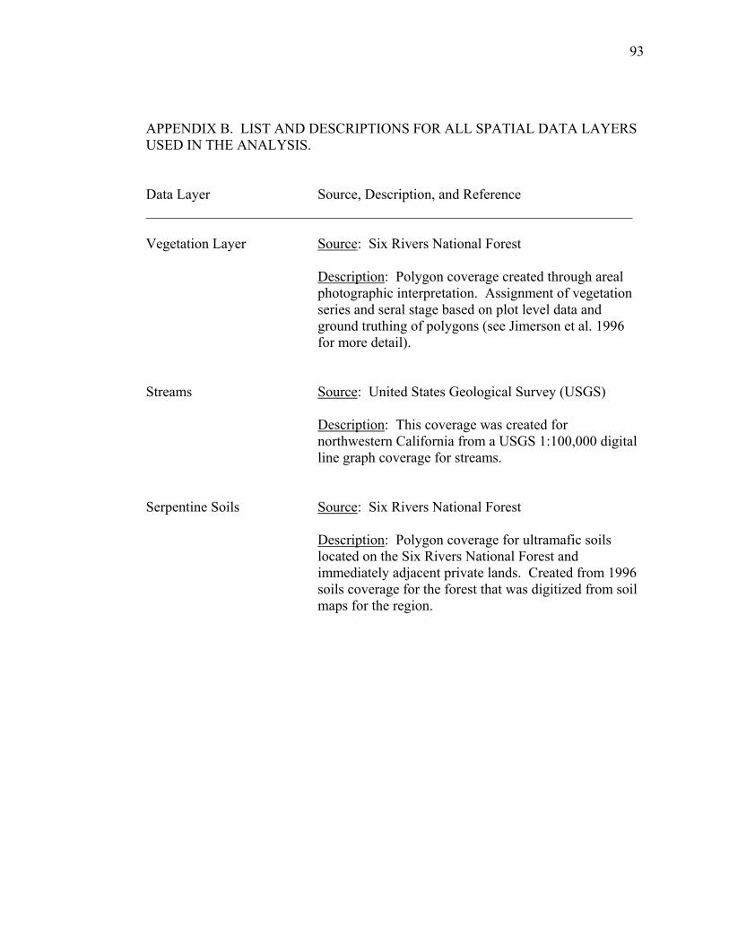
93

APPENDIX B. LIST AND DESCRIPTIONS FOR ALL SPATIAL DATA LAYERS USED IN THE ANALYSIS. Data Layer Source, Description, and Reference ____________________________________________________________________ Vegetation Layer Source: Six Rivers National Forest Description: Polygon coverage created through areal photographic interpretation. Assignment of vegetation series and seral stage based on plot level data and ground truthing of polygons (see Jimerson et al. 1996 for more detail). Streams Source: United States Geological Survey (USGS)

Description: This coverage was created for northwestern California from a USGS 1:100,000 digital line graph coverage for streams.

Serpentine Soils Source: Six Rivers National Forest Description: Polygon coverage for ultramafic soils located on the Six Rivers National Forest and immediately adjacent private lands. Created from 1996 soils coverage for the forest that was digitized from soil maps for the region.

94

APPENDIX C. SELECTED DESCRIPTIVE VARIABLES, LOG AND SNAG DATA FOR SERAL STAGES IN THE TANOAK AND DOUGLAS-FIR VEGETATION SERIES. ALL INFORMATiON PRESENTED IS FROM JIMERSON ET AL. 1996. SNAG AND LOG CLASSES ARE DEFINED BY DIAMETER (CM) AND HEIGHT OR LENGTH (M) COMBINATIONS, IN PARENTHESIS. MEANS AND STANDARD DEVIATIONS, IN PARENTHESIS, ARE PRESENTED. SERAL STAGE Vegetation Series Shub Pole Early-mature Mid-mautre Late-mature Old growth Variable ____________________________________________________________________________________________________________ Tanoak Series Snag Density (snags/hectare) _________________________________________________________________________________________________________ (>50.8 cm & 15.2 m) 0 0 0.24 (0.1) 0.64 (0.2) 0.24 (0.0) 0.64 (0.0) (>50.8 cm & 6 -15 m) 0 0 0.56 (0.2) 0.76 (0.3) 0.32 (0.1) 0.72 (0.0) (>50.8 & >6 m) 0 0 0.80 (0.2) 1.33 (0.4) 0.48 (0.1) 1.37 (0.1) _________________________________________________________________________________________________________ Snag Diameter (cm) __________________________________________________________________________________________________________ (>50.8 cm & 15.2 m) 0 0 76.7 (6.7) 71.1 (4.5) 110.9 (21.3) 92.9 (2.2) ((>50.8 cm & 6 -15 m ) 0 0 102.8 (11.1) 57.6 (4.8) 87.1 (1.5) 81.0 (2.7) (>50.8 & >6 m ) 0 0 86.6 (6.6) 66.8 (3.8) 105.6 (16.7) 88.9 (1.7) _________________________________________________________________________________________________________

95

SERAL STAGE Vegetation Series Shub Pole Early-mature Mid-mautre Late-mature Old growth Variable ____________________________________________________________________________________________________________ Douglas fir Series Snag Density (snags/hectare) __________________________________________________________________________________________________________ (>50.8 cm & 15.2 m) 0 0 0.24 (0.1) 0.12 (0.0) 0.36 (0.2) 0.97 (0.1) (>50.8 cm & 6 -15 m) 0 0 1.25 (0.6) 0.28 (0.2) 0.22 (0.1) 0.52 (0.1) (>50.8 & >6 m) 0 0 1.49 (0.6) 0.40 (0.2) 0.60 (0.2) 1.45 (0.1) __________________________________________________________________________________________________________ Snag Diameter (cm) __________________________________________________________________________________________________________ (>50.8 cm & 15.2 m) 0 0 82.5 (12.1) 61.4 (8.8) 84.5 (13.2) 86.6 (3.5) (>50.8 cm & 6 -15 m) 0 0 106.6 (5.8) 92.7 (11.1) 86.8 (7.8) 92.7 (9.3) (>50.8 & >6 m) 0 0 98.5 (6.0) 82.2 (9.3) 81.1 (11.4) 87.1 (3.3) __________________________________________________________________________________________________________

96

SERAL STAGE Vegetation Series Shub Pole Early-mature Mid-mautre Late-mature Old growth Variable ____________________________________________________________________________________________________________ Tanoak Series Log Density (logs/hectare) __________________________________________________________________________________________________________ (>76.2 cm) 2.26 (0.8) 3.27 (1.1) 2.14 (0.8) 0.72 (0.3) 0.08 (0.0) 1.74 (0.2) (>50.8 to 76.2 cm) 3.60 (1.1) 4.41 (1.2) 2.18 (0.7) 1.94 (0.8) 0.72 (0.3) 2.63 (0.2) __________________________________________________________________________________________________________ Douglas fir Series Log Density (logs/hectare) __________________________________________________________________________________________________________ (>76.2 cm) 3.28 (1.0) 1.98 (0.8) 4.86 (2.3) 0.85 (0.4) 0.28 (0.2) 1.54 (0.4) (>50.8 to 76.2 cm) 7.20 (1.7) 2.99 (1.2) 4.57 (1.9) 1.66 (0.5) 2.55 (0.7) 2.79 (0.7) __________________________________________________________________________________________________________

97

APPENDIX D. CALIFORNIA WILDLIFE HABITAT RELATIONSHIPS CLASSIFICATION RESULTS FOR EACH STATION. Eleven different CWHR habitat types were sampled, with marten detections

occurring in only 6 of these (Table 1). The majority of marten detections (24)

occurred in the Douglas-fir (9) and mixed hardwood-conifer (15) types. The highest

proportion of detections (2 of 3) occurred in the montane chaparral type. All 6 tree

size classes (1-6) and one shrub size class (3) were sampled, with marten detections

occurring in 5 of the six tree size classes and in the single shrub size class (Table 1).

Marten detections occurred most often in the larger tree size classes (3-6). All 4 tree

and 1 shrub canopy closure class were sampled, with marten detections occurring in

every class (Table 1). Marten detections in non-serpentine sites occurred almost

exclusively (27 of 28) in the dense (≥60%) tree canopy closure class, while detections

in serpentine sites occurred in all tree canopy closure classes.

98

Table D-1. California Wildlife Habitat Relationships results for all stations where martens were detected. Sample Unit- Ultramafic

Parent WHR Habitat WHR Size WHR Canopy

Station Material (Y/N) Type Class Closure

008-2 N DFR 6 Dense 018-1 N MHC 5 Dense 018-2 N MHC 5 Dense 032-1 N MRI 4 Dense 044-1 Y KMC 2 Sparse 045-1 N MHC 2 Dense 056-1 N MRI 3 Dense 058-2 Y MCP 3 Dense 059-1 Y KMC 3 Moderate 074-2 Y KMC 3 Open 077-1 N DFR 5 Dense 077-2 N MHC 4 Dense 078-1 N MHC 4 Dense 078-2 N MHC 4 Dense 084-1 N MHC 5 Dense 088-2 Y MCP 3 Dense 096-1 N MHC 6 Dense 098-1 N MHC 4 Dense 108-1 N DFR 5 Dense 109-1 N DFR 3 Dense 109-2 N MHC 3 Moderate 118-2 Y MHW 3 Dense 119-1 Y MHW 3 Dense 122-1 N MHC 6 Dense 122-2 N DFR 5 Dense 132-1 Y MHC 4 Dense 132-2 Y MHC 3 Dense 134-1 N MHC 5 Dense 150-1 N DFR 6 Dense 152-1 N DFR 4 Dense 152-2 N DFR 5 Dense 164-1 Y DFR 4 Dense 974-1 Y KMC 3 Open 995-1 N MHC 6 Dense

99

APPENDIX E. SAS CODE FOR AIC CALCULATION, ∆AIC, AND CHECK RESIDUALS FOR MODEL FIT. Adapted from SAS code written by J. Dunham and R. Reiman, Department of Fisheries and Wildlife, Oregon State University. OPTIONS LS=85 PS=60; *Read in data set; DATA Multi; INFILE 'K:\wild\carny\Slauson\Multi.csv' delimiter=','; INPUT SYSNO MAAM_det SHRUB_C SERAL_ST $ TREE_COV CONIF MASP MSP $ OG_COMP OLM_COMP OG_PCH OLM_PCH STREAM LOGGED SERP ; RUN; *Transform Aspect Data; DATA Multi; SET Multi; RETAIN pi 3.14159; aspect=MASP; radasp=((aspect+45)/360)*2*pi; cosasp=cos(radasp); RUN; *Print and review data for accuracy; PROC PRINT DATA=Multi; RUN; *Model Statement and AIC Calculation; %MACRO AIC (MODEL, CLASSVARS, XVARS); TITLE "&MODEL, &CLASSVARS, &XVARS"; *SPECIFY GENERAL STRUCTURE OF LOGISTIC REGRESSION MODEL OUTPUTING RELEVANT METRICS-MACRO REPLACES & WITH SPECIFIED VARIABLES WHEN CALLING MACRO ; PROC GENMOD DATA=Multi DESCENDING; CLASS MSP SERAL_ST; MODEL MAAM_det= &CLASSVARS &XVARS / DIST=BINOMIAL LINK=LOGIT LRCI; ODS OUTPUT MODELFIT=FITSTAT PARAMETERESTIMATES=PARMS MODELINFO=NUMOBS; OUTPUT OUT=OBSTAT PRED=PREDICT ; RUN; *SPECIFY LENGTH AND TYPE OF VARIABLES FROM ODS OUTPUT; DATA PARMS2 (DROP=df ChiSq ProbChiSq LowerCL UpperCL); LENGTH MODEL $8 XVARS $20 PARAMETER $20; *NOTE-- KEEP PARAMETER NAMES TO <= 20 CHARACTERS;

100

MODEL="&MODEL"; XVARS="&XVARS"; SET PARMS; IF ESTIMATE=0 AND STDERR=0 THEN DELETE; DROP LEVEL1; RUN; DATA NUMOBS2; LENGTH MODEL $8 XVARS $20; MODEL="&MODEL"; SET NUMOBS; *"GRABS" NOBS INFO FROM ODS OUTPUT (PROC PRINT ODS OUTPUT TO SEE THIS); IF LABEL1= 'Observations Used' then nobs=cVALUE1; IF NOBS NE . ; KEEP MODEL nobs; RUN; DATA FITSTAT2 (DROP=VALUEDF); LENGTH MODEL $8 XVARS $20 PARAMETER $20; MODEL="&MODEL"; XVARS="&XVARS"; SET FITSTAT; RUN; DATA TEMP; MERGE NUMOBS2 FITSTAT2; BY MODEL; RUN; *COMPUTE AICC FOR EACH MODEL; DATA MODELSUM; SET TEMP; IF CRITERION = 'Pearson Chi-Square' then k=NOBS-DF; RETAIN K; IF CRITERION='Log Likelihood' then AICC=-2*VALUE +2*K + (2*K*(K+1))/(NOBS-K-1); IF CRITERION='Log Likelihood'; DROP VALUE DF CRITERION XVARS; RUN; *FOR EACH ITERATION (i.e. MODEL SPECIFIED IN CALL STATEMENT) ADD RESULTS OF ABOVE TO A FILE (BASE=AICC) THAT KEEPS TRACK OF ALL ITERATIONS); PROC APPEND DATA=MODELSUM BASE=AICC FORCE; RUN; PROC APPEND DATA=PARMS2 BASE=PARAMEST FORCE; RUN;

101

*TO SEE WHAT THE ABOVE STEPS COMPLETED DO A PROC PRINT STATEMENT FOR THE ABOVE BASE FILES; *ENDS MACRO; %MEND; *Clear any previous output; PROC DATASETS LIBRARY=work MEMTYPE=ALL; DELETE AIC RP1-RP50; RUN; *CALL MACRO; SELECT EACH SCALE SET PLUS NULL MODEL AND RUN SEPARATELY %AIC (NULL, , ); %AIC (ST1_LTM, SERAL_ST cosasp*MSP, CONIF SHRUB_C ); %AIC (ST2_RLIT1, SERAL_ST cosasp*MSP, CONIF ); %AIC (ST3_RLIT2, cosasp*MSP, CONIF SHRUB_C ); %AIC (ST4_HSI, SERAL_ST , TREE_COV CONIF ); %AIC (ST5_COAST_S, SERAL_ST , SHRUB_C ); %AIC (ST6_2COAST_SC, SERAL_ST , CONIF SHRUB_C ); %AIC (ST7_3COAST_SCT, SERAL_ST cosasp*MSP, SHRUB_C ); %AIC (ST8_PAR_SHRUB, , SHRUB_C ); %AIC (ST9_2PAR_SERAL, SERAL_ST , ); %AIC (ST10_PURE_S, SERAL_ST , TREE_COV SHRUB_C ); %AIC (ST11_MESIC_CONIF, cosasp*MSP, CONIF ); %AIC (ST12_2MESIC_SHRUB, cosasp*MSP, SHRUB_C ); %AIC (ST13_3MESIC_SERAL, SERAL_ST cosasp*MSP, ); %AIC (ST14_TOTAL_COVER, , TREE_COV SHRUB_C ); %AIC (ST15_CLOSED_CONIF, , TREE_COV CONIF ); %AIC (LS1_PAR_SERALCOMP1, , OG_COMP ); %AIC (LS2_PAR_SERALCOMP2, , OLM_COMP ); %AIC (LS3_SERALC1_STREAM, , OG_COMP STREAM ); %AIC (LS4_SERALC2_STREAM, , OLM_COMP STREAM ); %AIC (LS5_SERALC1_SERPENTINE, , OG_COMP SERP ); %AIC (LS6_SERALC2_SERPENTINE, , OLM_COMP SERP ); %AIC (LS7_PAR_PATCH1, , OG_PCH ); %AIC (LS8_PAR_PATCH2, , OLM_PCH ); %AIC (LS9_LOGGING, , LOGGED ); %AIC (LS10_SERALC1_LOGGING, , OG_COMP LOGGED ); %AIC (LS11_SERALC2_LOGGING, , OLM_COMP LOGGED ); %AIC (LS12_PATCH1_LOGGING, , OG_PCH LOGGED ); %AIC (LS13_PATCH2_LOGGING, , OLM_PCH LOGGED ); %AIC (LS14_SERALC1_LOG_SERP, , OG_COMP LOGGED SERP ); %AIC (LS15_SERALC2_LOG_SERP, , OLM_COMP LOGGED SERP ); %AIC (LS16_SERALC1_LOG_STREAM, , OG_COMP LOGGED STREAM ); %AIC (LS17_SERALC2_LOG_STREAM, , OLM_COMP LOGGED STREAM ); %AIC (LS18_PATCH1_LOG_STREAM, , OG_PCH LOGGED STREAM ); %AIC (LS19_PATCH2_LOG_STREAM, , OLM_PCH LOGGED STREAM ); %AIC (LS20_PATCH1_LOG_SERP, , OG_PCH LOGGED SERP ); %AIC (LS21_PATCH2_LOG_SERP, , OLM_PCH LOGGED SERP );

102

%AIC (LS22_PATCH1_LOG_SERP_STREAM, , OG_PCH LOGGED SERP STREAM ); %AIC (LS23_PATCH2_LOG_SERP_STREAM, , OLM_PCH LOGGED SERP STREAM ); %AIC (LS24_PATCH1_SERPENTINE, , OG_PCH SERP ); %AIC (LS25_PATCH2_SERPENTINE, , OLM_PCH SERP ); %AIC (MS1_SHRUB_SERALC1, , OG_COMP SHRUB_C ); %AIC (MS2_SHRUB_SERALC2, , OLM_COMP SHRUB_C ); %AIC (MS3_SHRUB_PATCH1, , OG_PCH SHRUB_C ); %AIC (MS4_SHRUB_PATCH2, , OLM_PCH SHRUB_C ); %AIC (MS5_SHRUB_TREECOV_SERALC1, , OG_COMP TREE_COV SHRUB_C ); %AIC (MS6_SHRUB_TREECOV_SERALC2, , OLM_COMP TREE_COV SHRUB_C ); %AIC (MS7_SHRUB_TREECOV_PATCH1, , OG_PCH TREE_COV SHRUB_C ); %AIC (MS8_SHRUB_TREECOV_PATCH2, , OLM_PCH TREE_COV SHRUB_C ); %AIC (MS9_SHRUB_LOGGED, , SHRUB_C LOGGED ); %AIC (MS10_SERAL_LOGGED, SERAL_ST, LOGGED ); %AIC (MS11_SERAL_SHRUB_LOGGED, SERAL_ST, SHRUB_C LOGGED ); %AIC (MS12_SHRUB_SERALC1_LOG, , OG_COMP SHRUB_C LOGGED ); %AIC (MS13_SHRUB_SERALC2_LOG, , OLM_COMP SHRUB_C LOGGED ); %AIC (MS14_SHRUB_PATCH1_LOG, , OG_PCH SHRUB_C LOGGED ); %AIC (MS15_SHRUB_PATCH2_LOG, , OLM_PCH SHRUB_C LOGGED ); *THE BELOW STEPS TAKE SUMMARY INFO ON EACH MODEL TO GET AICC DIFFERENCES AND AKAIKE'S WEIGHTS; PROC SORT DATA=AICC; BY MODEL; RUN; PROC SORT DATA=PARAMEST; BY MODEL; RUN; DATA ALLTEST; MERGE AICC PARAMEST ; BY MODEL; IF PARAMETER= "Scale" THEN DELETE ; *A CLUNKY WAY TO GET THE MERGE STATEMENT TO ADD A VARIABLE TO EACH RECORD IS TO SET A DUMMY VARIABLE THAT YOU LATER "MERGE BY"; DUMMY=1; drop NOBS ; RUN; *FIND MIN AICC FROM SET OF MODELS AND OUTPUT IT FOR LATER MERGE; PROC MEANS DATA=ALLTEST MIN NOPRINT; VAR AICC; OUTPUT OUT=MINAKAIKE MIN=MINAICC; RUN; *GET PRELIMIMARY DATA FOR WEIGHTS WITH 1 RECORD PER MODEL; DATA MODELSUM; SET ALLTEST;

103

BY MODEL; *KEEPS ONLY THE FIRST RECORD OF EACH MODEL-- RECORDS PREVIOUSLY EXISTED FOR ALL PARAMETERS IN EACH MODEL; IF FIRST.MODEL; RUN; DATA MINAKAIKE; SET MINAKAIKE; *AGAIN, CLUNKY WAY OF SETTING UP MERGE; DUMMY=1; RUN; *INCLUDE MINAICC VALUE TO EACH RECORD OF SUMMARY OF AICC VALUES FOR EACH MODEL; DATA MODELSUM2; MERGE MINAKAIKE MODELSUM; BY DUMMY; *COMPUTE AICC DIFFERENCES; AICCDIF=AICC-MINAICC; *GET NUMERATOR OF EQUATION TO COMPUTE MODEL WEIGHTS (B&A PAGE 124); expdif= exp(-.5 * AICCDIF); DROP _TYPE_ _FREQ_ ; RUN; *GET DENOMINATOR OF EQUATION; PROC MEANS DATA=MODELSUM2 SUM NOPRINT; VAR EXPDIF; OUTPUT OUT=SUMEXPON SUM=SUMEXPD; RUN; DATA SUMEXPON; SET SUMEXPON; DUMMY=1; RUN; * COMPUTE AKAIKE'S WEIGHTS;

DATA MODELSUM3; MERGE MODELSUM2 SUMEXPON; BY DUMMY; w=expdif/sumexpd; run; DATA MODELSUM4; MERGE MODELSUM3 ALLTEST; BY MODEL; DROP _TYPE_ _FREQ_ EXPDIF SUMEXPD;

104

RUN; PROC PRINT DATA=MODELSUM4; RUN; * PRINT MODEL SUMMARY;

DATA MODELSUM_FINAL; SET MODELSUM4; BY MODEL; IF FIRST.MODEL; PROC PRINT ; VAR MODEL K AICC AICCDIF W; RUN; *TO GET AICC AND MODEL WEIGHTS FOR EACH MODEL AND THE PAR EST (SE)FOR EACH PARAM FROM EACH MODEL; PROC PRINT DATA=MODELSUM4; RUN; *Residual check for all models; %MACRO RESCHECK (MODEL, CLASSVARS, XVARS); TITLE "Model, &CLASSVARS, &XVARS"; TITLE2 "Multi"; PROC GENMOD DATA=Multi DESCENDING; *CLASS &CLASSVARS; CLASS MSP SERAL_ST; MODEL MAAM_det= &CLASSVARS &XVARS / DIST=BINOMIAL LINK=LOGIT LRCI obstats residuals; *OUTPUT OUT=predout; ods output obstats=obstats2 residuals=RESID; RUN; PROC PRINT DATA=OBSTATS2; RUN; proc plot data=obstats2 vpercent=50; plot RESID*(PRED &XVAR)/VREF=0; RUN; %MEND; GOPTIONS NODISPLAY COLORS=(BLACK) GOUTMODE=APPEND; PROC GPLOT DATA=predout GOUT=RP; PLOT RESID*(PRED &XVARS); RUN; QUIT; GOPT ONS DISI PLAY; PROC GREPLAY IGOUT=RP NOFS TEMPLATE=twoxtwo TC=template; TDEF twoxtwo

105

1/ ULX=0 ULY=100 URX=50 URY=100 LLX=0 LLY=50 LRX=50 LRY=50 2/ COPY=1 XLATEX=50 3/ COPY=1 XLATEY=-50 4/ COPY=3 XLATEX=50; TREPLAY 1:1 2:2 3:3 4:4; RUN; QUIT; %MEND; *Submit this for all models in the set; *%RESCHECK (POS.SERAL.SHRUB, SERAL_STAND , SHRUB_COV ); %RESCHECK (NULL, , ); %RESCHECK (ST1_LTM, SERAL_ST cosasp*MSP, CONIF SHRUB_C ); %RESCHECK (ST2_RLIT1, SERAL_ST cosasp*MSP, CONIF ); %RESCHECK (ST3_RLIT2, cosasp*MSP, CONIF SHRUB_C ); %RESCHECK (ST4_HSI, SERAL_ST , TREE_COV CONIF ); %RESCHECK (ST5_COAST_S, SERAL_ST , SHRUB_C ); %RESCHECK (ST6_2COAST_SC, SERAL_ST , CONIF SHRUB_C ); %RESCHECK (ST7_3COAST_SCT, SERAL_ST cosasp*MSP, SHRUB_C ); %RESCHECK (ST8_PAR_SHRUB, , SHRUB_C ); %RESCHECK (ST9_2PAR_SERAL, SERAL_ST , ); %RESCHECK (ST10_PURE_S, SERAL_ST , TREE_COV SHRUB_C ); %RESCHECK (ST11_MESIC_CONIF, cosasp*MSP, CONIF ); %RESCHECK (ST12_2MESIC_SHRUB, cosasp*MSP, SHRUB_C ); %RESCHECK (ST13_3MESIC_SERAL, SERAL_ST cosasp*MSP, ); %RESCHECK (ST14_TOTAL_COVER, , TREE_COV SHRUB_C ); %RESCHECK (ST15_CLOSED_CONIF, , TREE_COV CONIF ); %RESCHECK (LS1_PAR_SERALCOMP1, , OG_COMP ); %RESCHECK (LS2_PAR_SERALCOMP2, , OLM_COMP ); %RESCHECK (LS3_SERALC1_STREAM, , OG_COMP STREAM ); %RESCHECK (LS4_SERALC2_STREAM, , OLM_COMP STREAM ); %RESCHECK (LS5_SERALC1_SERPENTINE, , OG_COMP SERP ); %RESCHECK (LS6_SERALC2_SERPENTINE, , OLM_COMP SERP ); %RESCHECK (LS7_PAR_PATCH1, , OG_PCH ); %RESCHECK (LS8_PAR_PATCH2, , OLM_PCH ); %RESCHECK (LS9_LOGGING, , LOGGED ); %RESCHECK (LS10_SERALC1_LOGGING, , OG_COMP LOGGED ); %RESCHECK (LS11_SERALC2_LOGGING, , OLM_COMP LOGGED ); %RESCHECK (LS12_PATCH1_LOGGING, , OG_PCH LOGGED ); %RESCHECK (LS13_PATCH2_LOGGING, , OLM_PCH LOGGED ); %RESCHECK (LS14_SERALC1_LOG_SERP, , OG_COMP LOGGED SERP ); %RESCHECK (LS15_SERALC2_LOG_SERP, , OLM_COMP LOGGED SERP ); %RESCHECK (LS16_SERALC1_LOG_STREAM, , OG_COMP LOGGED STREAM ); %RESCHECK (LS17_SERALC2_LOG_STREAM, , OLM_COMP LOGGED STREAM ); %RESCHECK (LS18_PATCH1_LOG_STREAM, , OG_PCH LOGGED STREAM ); %RESCHECK (LS19_PATCH2_LOG_STREAM, , OLM_PCH LOGGED STREAM ); %RESCHECK (LS20_PATCH1_LOG_SERP, , OG_PCH LOGGED SERP ); %RESCHECK (LS21_PATCH2_LOG_SERP, , OLM_PCH LOGGED SERP ); %RESCHECK (LS22_PATCH1_LOG_SERP_STREAM, , OG_PCH LOGGED SERP STREAM );

106

%RESCHECK (LS23_PATCH2_LOG_SERP_STREAM, , OLM_PCH LOGGED SERP STREAM ); %RESCHECK (LS24_PATCH1_SERPENTINE, , OG_PCH SERP ); %RESCHECK (LS25_PATCH2_SERPENTINE, , OLM_PCH SERP ); %RESCHECK (MS1_SHRUB_SERALC1, , OG_COMP SHRUB_C ); %RESCHECK (MS2_SHRUB_SERALC2, , OLM_COMP SHRUB_C ); %RESCHECK (MS3_SHRUB_PATCH1, , OG_PCH SHRUB_C ); %RESCHECK (MS4_SHRUB_PATCH2, , OLM_PCH SHRUB_C ); %RESCHECK (MS5_SHRUB_TREECOV_SERALC1, , OG_COMP TREE_COV SHRUB_C ); %RESCHECK (MS6_SHRUB_TREECOV_SERALC2, , OLM_COMP TREE_COV SHRUB_C ); %RESCHECK (MS7_SHRUB_TREECOV_PATCH1, , OG_PCH TREE_COV SHRUB_C ); %RESCHECK (MS8_SHRUB_TREECOV_PATCH2, , OLM_PCH TREE_COV SHRUB_C ); %RESCHECK (MS9_SHRUB_LOGGED, , SHRUB_C LOGGED ); %RESCHECK (MS10_SERAL_LOGGED, SERAL_ST, LOGGED ); %RESCHECK (MS11_SERAL_SHRUB_LOGGED, SERAL_ST, SHRUB_C LOGGED ); %RESCHECK (MS12_SHRUB_SERALC1_LOG, , OG_COMP SHRUB_C LOGGED ); %RESCHECK (MS13_SHRUB_SERALC2_LOG, , OLM_COMP SHRUB_C LOGGED ); %RESCHECK (MS14_SHRUB_PATCH1_LOG, , OG_PCH SHRUB_C LOGGED ); %RESCHECK(MS15_SHRUB_PATCH2_LOG, , OLM_PCH SHRUB_C LOGGED );

107

APPENDIX F. UNIVARIATE DESCRIPTIVE STATISTICS FOR EACH CONTINUOUS STAND AND HOME RANGE SCALE VARIABLE. Table F-1. Univariate descriptive statistics for stand scale variables. ___________________________________________________________________ Variable Mean (SD) Detection (n=26) Non-detection (n=133) ___________________________________________________________________ % Shrub Cover 74.4% (21.3) 47.4% (26.8) Non-serpentine 73.5% (22.3) 43.8% (25.5) Serpentine 76.1% (20.3) 75.6% (19.5) Tree Canopy Closure 72.6% (27.6) 72.0% (23.4) Non-serpentine 85.8% (9.0) 74.4% (22.0) Serpentine 47.7% (33.9) 53.3% (26.0) % Relative Conifer 82.0% (17.2) 70.2% (29.1) Non-serpentine 74.7% (16.4) 67.1% (29.2) Serpentine 96.0% (7.4) 94.3% (11.9) ___________________________________________________________________ *Sample sizes for detections and non-detections at non-serpentine (n = 15, n = 118) and serpentine (n = 9, n = 17) stands.

108

Table F-2. Univariate descriptive statistics for home-range scale variables. ___________________________________________________________________ Variable Mean (SD) Detection (n=26) Non-detection (n=133) ___________________________________________________________________ Old Growth Composition 75.2 Ha (54.5) 55.5 Ha (51.3) Non-serpentine 91.2 Ha (48.6) 56.0 Ha (51.3) Serpentine 45.0 Ha (54.8) 50.9 Ha (53.2) OG and LM Composition 139.0 Ha (58.1) 113.3 Ha (71.3) Non-serpentine 166.6 Ha (42.5) 115.2 Ha (74.1) Serpentine 86.7 Ha (47.4) 97.8 Ha (41.2) Largest OG Patch 64.3 Ha (49.8) 41.2 Ha (43.5)

Non-serpentine 78.1 Ha (43.2) 42.4 Ha (45.5) Serpentine 38.3 Ha (53.4) 31.3 Ha (20.5) Largest OG and LM Patch 113.5 Ha (64.8) 86.3 Ha (67.5) Non-serpentine 141.6 Ha (51.1) 88.2 Ha (70.1) Serpentine 60.5 Ha (55.4) 70.9 Ha (40.2) Amount of Serpentine 95.9 Ha (124.7) 31.4 Ha (64.8) Non-serpentine 9.6 Ha (22.9) 13.1 Ha (31.3) Serpentine 258.8 Ha (43.3) 174.9 Ha (81.1) Amount of Riparian 2293 m (1355) 2186 m (1438) Non-serpentine 2570 m (1410) 2125 m (1462) Serpentine 1770 m (1135) 2669 m (1155) Amount Logged 15.6 % (15.8) 30.7 % (36.3) Non-serpentine 18.2 % (18.3) 33.4 % (37.5) Serpentine 10.6 % (8.2) 9.2 % (12.4) __________________________________________________________________

109

APPENDIX G. SUMMARY OF POTENTIAL NATURAL VEGETATION (PNV) SERIES AND SUBSERIES FOR STANDS SAMPLED. PNV Type (Code) Total # Sampled Marten Detections Subseries (Code) ________________________________________________________________

Tanoak Series (00) 76 16 ____________________________________________________________ LIDE2-CHLA (0001) 3 1 LIDE2-QUCH2 (0017) 14 2 LIDE2-CACH2 (0019) 21 4 LIDE2-ACER (0023) 2 1 LIDE2-VAOV (0038) 22 5 LIDE2-GASH (0039) 12 2 LIDE2-DRY SHRUB (0041) 2 1 ____________________________________________________________

Port-Orford Cedar Series (01) 1 0

_________________________________________________________________ CHLA-ABC0 (0102) 1 ____________________________________________________________

White Fir Series (02) 20 0 ____________________________________________________________ ABCO-ABCO (0202) 1 ABCO-ABMAS (0203) 2 ABCO-PSME (0205) 14 ABCO-LIDE3 (0216) 1 ABCO-PIBR (0218) 1 ABCO-CACH2 (0219) 1 ____________________________________________________________

Red Fir Series (03) 2 0

_________________________________________________________________ ABMAS-PIMO3 (0315) 1 ABMAS-PIBR (0318) 1 ____________________________________________________________

110

PNV Type (Code) Total # Sampled Marten Detections Subseries (Code) ________________________________________________________________

Jeffrey Pine Series (04) 5 0

_________________________________________________________________ PIJE-PSME (0405) 1 PIJE-LIDE3 (0416) 4 ___________________________________________________________

Douglas-fir Series (05) 35 5 ___________________________________________________________

PSME-QUCH2 (0517) 5 0

PSME-CACH2 (0519) 19 4 PSME/QUVA (0542) 11 1 ___________________________________________________________

Sugar Pine Series (09) 1 0 ___________________________________________________________ PILA-PIMO3 (0915) 1 ___________________________________________________________

Redwood Series (14) 13 0

________________________________________________________________ Unknown (1400) 8 SESE2-XXX (1401) 3 SESE2-PSME (1405) 2 ___________________________________________________________

Western White Pine (15) 9 5

________________________________________________________________ PIMO3-PSME (1505) 3 1 PIMO3-PICO1 (1506) 6 4 ___________________________________________________________

Riparian (28) 1 0

________________________________________________________________ UNKNOWN (2899) 1 ___________________________________________________________

111

Species Codes: ABCO: white fir, ABMAS: red fir, ACER: maple sp., CACH2: chinquapin, CHLA: Port-Orford Cedar, GASH: salal, LIDE2: tanoak, LIDE3: Incense cedar, PIBR: Brewer’s spruce, PICO1: lodgepole pine, PIJE: Jeffrey pine, PILA: sugar pine, PIMO3: Western white pine, PSME: Douglas-fir, QUCH2: canyon live oak, QUVA: huckleberry oak, SESE2: redwood, VAOV Figure G-1. Percent used and available for the five most frequently sampled vegetation series.

112

Figure G-2. Seral stage distribution by vegetation series for all 159 sampled stands.