Growth and Trade with Frictions:

A Structural Estimation Framework∗

James E. Anderson Mario Larch

Boston College and NBER University of Bayreuth

Yoto V. Yotov

Drexel University

February 8, 2016

Abstract

We build and estimate a structural dynamic general equilibrium model of growth andtrade. Gravity is combined with a capital accumulation mechanism driving transitionbetween steady states. Trade aects growth through changes in consumer and producerprices that stimulate or impede physical capital accumulation. Simultaneously, growthaects trade, directly through changes in country size and indirectly through changesin the incidence of trade costs. Theory maps to an econometric system that identiesthe structural parameters of the model. Counterfactual trade liberalization magniesstatic gains on the discounted path to the steady state by a dynamic path multiplier ofaround 1.6.

JEL Classication Codes: F10, F43, O40

Keywords: Trade, Growth, Income, Trade Liberalization, Capital Accumulation.

∗Contact information: Andersonjames.anderson@bc.edu; Larchmario.larch@uni-bayreuth.de; Yotovyotov@drexel.edu.

Acknowledgements: We thank Costas Arkolakis, Eric Bond, Holger Breinlich, SvetlanaDemidova, Klaus Desmet, Jonathan Eaton, Markus Eberhardt, Carsten Eckel, HartmutEgger, Giovanni Facchini, Gabriel Felbermayr, Joseph Francois, Gene Grossman, BurkhardHeer, Benedikt Heid, Marten Hillebrand, Richard Hule, Giammario Impullitti, Oleg Itskhoki,Dalia Marin, Xenia Matschke, Thierry Mayer, Daniel Millimet, Eduardo Morales, JulianEmami Namini, Peter Neary, Douglas Nelson, Dennis Novy, Ezra Obereld, Thomas Os-ang, Veronica Rappoport, Stephen Redding, Raymond Riezman, Esteban Rossi-Hansberg,Thomas Sampson, Serge Shikher, Michael Sposi, David Stadelmann, Andrey Stoyanov,Costas Syropoulos, Felix Tintelnot, Klaus Wälde, Kei-Mu Yi, and participants at the SIREWorkshop on Theory and Estimation of Gravity Equations 2013, Glasgow, the Allied So-cial Science Associations Annual Meeting 2014, Philadelphia, the Midwest InternationalEconomics Group Spring 2014 Meeting, Indianapolis, the SIRE Workshop on Country Sizeand Border Eects in a Globalised World 2014, Edinburgh, the CESifo Workshop on Re-gional Mega Deals: New Trends, New Models, New Insights 2014, Venice, the Conferenceon Research on Economic Theory and Econometrics 2014, Milos, the 29th Annual Congressof the European Economic Association 2014, Toulouse, the 16th Annual Congress of the Eu-ropean Trade Study Group 2014, Munich, the Annual Meeting of the Society for EconomicDynamics 2015, Warsaw, the Panel Data Workshop on International Trade, University ofAmsterdam 2015, the Annual Congress of the Research Committee on International Eco-nomics of the German Economic Society 2015, Tübingen, the CESifo Area Conference onGlobal Economy 2015, Munich, the XX. Conference on Dynamics, Economic Growth, andInternational Trade 2015, Geneva, and seminars at Drexel University, Temple University,the Centre for Trade and Economic Integration at the Graduate Institute, Geneva, theEconomics Research Institute at the Bulgarian Academy of Sciences, the World Trade Or-ganization, Princeton University, Ludwig-Maximilian University in Munich, University ofBayreuth, McMaster University, York University, the U.S. International Trade Commission,University of Trier, University of Salzburg, CEP/LSE, University of Mainz, the AustrianInstitute of Economic Research (WIFO), Vienna, and the Vienna University of Economicsand Business for valuable comments and suggestions. Mario Larch is grateful for nancialsupport under the Fritz Thyssen Stiftung grant No. Az. 50.14.0.013.

1 Introduction

The relationship of trade and growth has been a central concern of economists since Adam

Smith. More than two centuries later debate continues about an empirically strong rela-

tionship between trade and growth, in contrast to professional consensus about static gains

from trade.1 Despite academic doubts, policy analysts and negotiating parties on both sides

of trade mega deals such as the Transatlantic Trade and Investment Partnership (TTIP)

between the United States and the European Union expect that TTIP will result in more

jobs and growth.2 These observations motivate our development of a dynamic model of

trade and transitional capital accumulation that allows structural estimation. Accumulation

eects are big. Counterfactual simulations of two dierent trade liberalization experiments

with the tted model yield discounted dynamic gains over the path to the steady state that

are more than 60% larger than static gains, a dynamic path multiplier around 1.6. Multi-

pliers do not vary much with economy size, in contrast to the static gains that are larger in

smaller economies.

The model features many countries that are asymmetric in size, in bilateral trade frictions

and in capital accumulation frictions. The CES Armington trade gravity model is combined

with a Lucas and Prescott (1971) capital accumulation model of transition between steady

states. Two frictions interact on stage: costly trade and costly capital adjustment. Capital

1In order to motivate their famous paper, Frankel and Romer (1999) note that [d]espite the great eortthat has been devoted to studying the issue, there is little persuasive evidence concerning the eect of tradeon income. Similarly, Baldwin (2000) conrms that [t]he relationships between trade and growth have longbeen a subject of [study and] controversy among economists. This situation continues today.Better models could help, but Head and Mayer (2014) note that the best tting trade model (gravity) is

static, and This raises the econometric problem of how to handle the evolution of trade over time in responseto changes in trade costs. (Head and Mayer, 2014, p. 189). Similarly, Desmet and Rossi-Hansberg (2014b)note that introducing dynamics to static multi-country trade models adds considerable complexity because:(i) consumers care about the distribution of their economic activities not only over countries, but also overtime; and (ii) the clearance of goods and factor markets is dicult, as prices depend on international trade.These two diculties typically make spatial dynamic models intractable, both analytically and numerically.(Desmet and Rossi-Hansberg, 2014b, p. 1212).

2Press release, Brussels, 28 January 2014, http://trade.ec.europa.eu/doclib/press/index.cfm?id=1020.President Obama of U.S. and Minister Rajoy of Spain also agreed that there is enormous potential forTTIP to increase trade and growth between two of the largest economic actors in the world. (Oceof the Press Secretary, White House, January, 2014, http://iipdigital.usembassy.gov/st/english/texttrans/2014/01/20140114290784.html#axzz2u59pirmD.)

1

stock adjustment in each country is subject to iceberg trade costs because capital requires

imports, but in addition costly adjustment cost and depreciation act essentially like iceberg

frictions on the intertemporal margin. Forbidding complexity is reduced by our choice of

structure. At each point in time bilaterally varying iceberg trade frictions are consistently

aggregated into productivity shifters in the form of national multilateral resistances. Over

time, the log-linear utility and log-linear capital transition function setup of Lucas and

Prescott (1971) and Hercowitz and Sampson (1991) applied here yields a closed-form solution

for optimal accumulation by innitely lived representative agents with perfect foresight.3 The

closed-form solution for accumulation is the bridge to structural estimation of a log-linear

econometric system.4

The estimated model allows quantication of the causal eect of openness on income

and growth. It also provides all the key structural parameters needed to simulate coun-

terfactuals with the model.5 Counterfactual liberalization experiments with the estimated

model decompose and quantify the various channels through which trade aects growth and

through which growth impacts trade. To compare dynamic gains from liberalization with

a static alternative, we follow Lucas (1987) to calculate the constant fraction of aggregate

consumption in each year that consumers would need to be paid in the baseline case to give

them the same utility they obtain from the consumption stream in the counterfactual.

Our model adds dynamics to the family of new quantitative static trade models, such

as Eaton and Kortum (2002) and Anderson and van Wincoop (2003) (as summarized in

3More recently, the log-linear capital transition function was, for example, used by Eckstein et al. (1996)to synthesize exogenous and endogenous sources of economic growth, by Kocherlakota and Yi (1997) toinvestigate whether permanent changes in government policies have permanent eects on growth rates, andby Abel (2003) to investigate the eects of a baby boom on stock prices and capital accumulation.

4In contrast, no closed-form solution is available for models in the spirit of the dynamic, stochastic,general equilibrium (DSGE) open economy macroeconomics literature, such as Backus et al. (1992, 1994).In our robustness analysis (see online Appendix C.3) we experiment with alternative specications for capitalaccumulation. While these do not lead to the convenient and tractable closed-form solution from our mainanalysis, they do generate qualitatively identical and quantitatively similar results.

5The internal consistency of parameter estimates with the data basis of counterfactual exercises is a keyadvantage of our approach: we test for the hypothesized link's signicance and use reasonably precise pointestimates to quantify the links in simulations. Our system delivers estimates of the trade elasticity, of thecapital (labor) share in production, of the capital depreciation rate, and of bilateral trade costs, which areall comparable to corresponding values from the existing literature.

2

Costinot and Rodríguez-Clare, 2014).6 Our model is also related to two notable eorts to

introduce dynamics within a heterogeneous spatial framework. First, Krusell and Smith,

Jr. (1998) show that in macroeconomic models with heterogeneity features, aggregate vari-

ables (i.e., consumption, capital stock, and relative prices) can be approximated very well

as a function of the mean of the wealth distribution and an aggregate productivity shock.

Second, Desmet and Rossi-Hansberg (2014b) deliver a tractable dynamic framework, where

the rm's dynamic decision to innovate reduces to a sequence of static prot-maximization

problems, by imposing structure that disciplines the mobility of labor, land-ownership by

the rm, and the diusion of technology.7 Similar to Desmet and Rossi-Hansberg (2014b),

we oer an analytical solution to the consumer's dynamic decision to invest. An important

dierence between these models and ours is that the models of Krusell and Smith, Jr. (1998)

and Desmet and Rossi-Hansberg (2014b) are stochastic whereas ours is deterministic. With-

out stochastic shocks, our optimization problem boils down to solving a non-linear equation

system between the steady states. Added tractability comes from gravity structure that

consistently aggregates bilateral trade frictions for each country into multilateral resistance

indexes. This second feature is similar to Krusell and Smith, Jr. (1998), but replaces an

approximation with an exact ideal index based on the structure of the system. We abstract

from non-zero steady-state growth for simplicity.8 We also abstract from endogenous tech-

nological change, but changes in multilateral resistance are eectively a type of endogenous

6In doing so, we extend an earlier literature (i.e., Solow, 1956; Acemoglu and Zilibotti, 2001; Acemoglu andVentura, 2002; Alvarez and Lucas, Jr., 2007), and we complement some new inuential papers (i.e., Sampson,2014; Eaton et al., 2015) that study the dynamics of trade. These studies calibrate their models in arguablymore complex environments. In contrast, we deliver a structural econometric system that allows us to testand establish causal relationships between trade, income, and growth and delivers the key parameters thatwe employ in our counterfactual analysis. The price of this estimatability is a focus on capital accumulationas the single channel for transmitting dynamic eects along with convenient functional form assumptions.

7The usefulness of this approach is shown by Desmet and Rossi-Hansberg (2014a) who apply it to studythe geographic impact of climate change, and Desmet et al. (2015) who develop a dynamic spatial growththeory with realistic geography to study the eects of migration and of a rise in the sea level.

8Growth in our framework is exclusively driven by capital accumulation. Please see the literature reviewSection 2 for motivation of this choice. Further, consistent with the description of the role of capital accu-mulation in transitional dynamics in Grossman and Helpman (1991), our framework generates transitionalbut not steady-state growth. Thus, if not mentioned explicitly otherwise, when we use the term growthwe have in mind capital accumulation between steady states.

3

technological change.

The structural gravity setup of Anderson and van Wincoop (2003) based on constant

elasticity of substitution (CES) preferences over products dierentiated by place of origin

(Armington, 1969) forms the trade module of the model.9 Recent work by Arkolakis et al.

(2012, henceforth also ACR) argues that gains from trade measures in such models represent

a general class of models for which the key parameter is a single trade elasticity. This class

of models readily integrates with our model of capital accumulation. Capital itself is an

alternative use of the consumable bundle. In the steady state, the accumulation ow osets

depreciation, essentially equivalent to a composite intermediate good. In this sense the model

is isomorphic to Eaton and Kortum (2002) but with substitution on the intensive margin. An

extension to incorporate intermediate goods following Eaton and Kortum (2002) conrms

that qualitative properties are the same while quantitative results shift signicantly.

We implement the dynamic structural gravity model on a sample of 82 countries over

the period 19902011. First, we translate the model into a structural econometric system

that oers a theoretical foundation to and expands the famous reduced-form specication

of Frankel and Romer (1999). In addition, we complement Frankel and Romer (1999) and

a series of other studies by proposing a novel structural instrument in order to identify

the eects of trade openness on income.10 Similar to Frankel and Romer (1999) and other

related studies, we identify a signicant causal eect of trade on income. In addition, we

complement the trade-and-income system of Frankel and Romer with a structural equation

9The gravity model is the workhorse in international trade. Anderson (1979) is the rst to build a gravitytheory of trade based on CES preferences with products dierentiated by place of origin. Bergstrand (1985)embeds this setup in a monopolistic competition framework. More recently, Eaton and Kortum (2002),Helpman et al. (2008), and Chaney (2008) derived structural gravity based on selection (hence substitutionon the extensive margin) in a Ricardian framework. Thus, as noted by Eaton and Kortum (2002) andArkolakis et al. (2012), a large class of models generate isomorphic gravity equations. Anderson (2011) andCostinot and Rodríguez-Clare (2014) summarize the alternative theoretical foundations of economic gravity.

10Notable studies that propose alternative instruments for trade/trade openness in Frankel-Romer settingsinclude Redding and Venables (2004), that uses a version of their market access index, Feyrer (2009b), thatproposes a new time-varying geographic instrument which capitalizes on the fact that country pairs withrelatively short air routes have beneted more from improvements in technology, Feyrer (2009a), that exploitsthe closing of the Suez canal as a natural experiment, Lin and Sim (2013), that constructs a new measureof trade cost based on the Baltic Dry Index, and Felbermayr and Gröschl (2013), that uses natural disastersas an instrument. See Sections 4.1.2 and 4.3.2 for further details and performance of our instrument.

4

that captures the eects of trade openness on capital accumulation. The estimation of our

structural system yields estimates of all but one of the model parameters.

Two counterfactual liberalization experiments quantify and decompose the relationships

between growth and trade, each based on the newly constructed trade costs combined with

data on the rest of the variables in our model. These experiments reveal that the dynamic

eects of trade liberalization lead to an over 60 percent increase in the corresponding static

eects, implying a dynamic path multiplier of around 1.6.

In the NAFTA experiment, average welfare for the North American Free Trade Agreement

(NAFTA) members increases from 1.265% to 2.056%. Following Estevadeordal and Taylor

(2013), we calculate a yearly growth rate eect of NAFTA for the rst 15 years of adjustment

of about 0.368%, while for the non-NAFTA countries we nd a small negative eect of

−0.002%. Hence, our framework implies an acceleration in growth rates of real gross domestic

product (GDP) in NAFTA countries compared to non-NAFTA countries of about 0.3693%

per year for the rst 15 years after the implementation of NAFTA.11 The dynamic channels

in our framework (increased country size and changes in the multilateral resistances) imply

that preferential trade liberalization (e.g. a Regional Trade Agreement, RTA) may benet

non-members eventually, despite the initial negative eect of trade diversion. RTAs benet

members and stimulate growth by making investment more attractive. This will normally

lead to lower sellers' incidence for member countries, but also to lower buyers' incidence in

non-members. Furthermore, the increased income in member countries will translate into

an increase of imports from all trading partners, including non-members. Consistent with

that logic, our simulation of NAFTA shows that its formation had small and non-monotonic

negative trade eects on non-member countries and even some small net trade-creation eects

11Estevadeordal and Taylor (2013) use a small open developing economy model to motivate their empiricaldierence equation. They use a treatment-and-control approach to compare the acceleration in growthrates of real GDP in liberalizing countries compared to non-liberalizing countries. The main nding is adierence in the two groups' trends of about 1% per year. Our comparable nding of 0.37% is based on astructural model taking care of all general equilibrium eects which is not possible with a treatment-and-control approach and potentially biasing the results substantially (see Heckman and Taber, 1998). Sampson(2014) nds in a setting with heterogeneous rms that the dynamic eects of trade liberalization triple.

5

for several non-members (e.g. the Netherlands). A battery of sensitivity checks conrms the

robustness of our results.

A globalization experiment examines the eect of a uniform fall in international trade

costs of 6.4%. All countries gain, smaller ones gain more, and the dynamic path multiplier

is around 1.6 for all countries despite the big dierences in size.

The rest of the paper is organized as follows. In section 2 we present our contributions in

relation to existing studies. Section 3 develops the theoretical foundation and discusses the

structural links between growth and trade in our model. In Section 4, we translate our the-

oretical framework into an econometric model. Section 5 oers counterfactual experiments.

Section 6 concludes with some suggestions for future research. All derivations, technical

discussions and robustness experiments can be found in the online Appendix.

2 Relation to Literature

Our work contributes to several inuential strands of the literature. First, we build a bridge

between the empirical and theoretical literature on the links between growth and trade. The

seminal work of Frankel and Romer (1999) uses a reduced-form framework to study the

relationships between income and trade.12 Wacziarg (2001) investigates the links between

trade policy and economic growth employing a panel of 57 countries for the period of 1970 to

1989. A key nding is that physical capital accumulation accounts for about 60% of the total

positive impact of openness on economic growth. Baldwin and Seghezza (2008) and Wacziarg

and Welch (2008) conrm these ndings for up to 39 countries for two years (1965 and 1989)

and a set of 118 countries over the period 1950 to 1998, respectively. Cuñat and Maezzoli

(2007) demonstrate the role of factor accumulation to reproduce the large observed increases

in trade shares after modest tari reductions. These studies motivate our focus on capital

accumulation as the source of growth in our model.13 We extend this literature in three

12In order to account for the endogeneity problems that plague the relationships between income andtrade, Frankel and Romer (1999) draw from the early, a-theoretical gravity literature (see Tinbergen, 1962)and propose to instrument for trade ows with geographical characteristics and country size.

13The correlation in our sample between changes in trade openness (measured as exports plus imports asshare of gross domestic product) and changes in capital accumulation is about 0.38 (p-value 0.002).

6

ways. First, we oer a theoretical equation that corresponds directly to the reduced-form

specication of Frankel and Romer (1999). Second, we propose a novel structural instrument

for trade openness. Third, we introduce a theoretically-motivated equation that captures the

eects of trade on capital accumulation and hence growth.

On the structural trade-and-growth side, our paper is related to a series of inuential

papers by Jonathan Eaton and Samuel Kortum (see Eaton and Kortum, 2001, 2002, 2005),14

who study the links between trade, production and growth via technological spill-overs.

We abstract from the random productivity draws setup of Eaton and Kortum (EK) for

simplicity, since the EK model is observationally equivalent to the structural gravity model

we estimate. This simplicity allows our addition of capital accumulation in transition. The

steady state of our model is equivalent to EK if we add a ow use of intermediate goods to

the ow of capital to oset depreciation. While the relationships between growth and trade

are of central interest in this paper and in Eaton and Kortum's work, we view our study as

complementary to Eaton and Kortum's agenda because the dynamic relationships between

trade and production in our model are generated via capital accumulation.15

Our approach is related to recent inuential work by Eaton et al. (2015), EKNR hereafter.

We share with EKNR the common elements of a gravity structure and capital accumulation

specied as a perfect foresight Cobb-Douglas adjustment process as in Lucas and Prescott

(1971). We dier in imposing the polar case of nancial autarky in contrast to the complete

markets polar case of EKNR and, less essentially, in assuming one good in contrast to the

four goods of EKNR. Our strategy of simplication attains an estimable system focused

14The work of Eaton and Kortum that is most closely related to our study is thoroughly summarized in theirmanuscript Eaton and Kortum (2005). Most relevant to our work are their chapters ten and eleven, whichstudy how trade in capital goods possibly transmits technological advances and investigate the geographicalscope of technological progress in a multi-country (semi)endogenous growth framework, respectively. Fora thorough review of the earlier theoretical literature on trade and (endogenous) technology, we refer thereader to Grossman and Helpman (1995). More recent developments include Acemoglu and Zilibotti (2001),Acemoglu and Ventura (2002), Alvarez and Lucas, Jr. (2007), Sampson (2014), and Eaton et al. (2015).

15Even though technology is exogenous in our model, our framework has implications for TFP calculationsand estimations. In particular, the introduction of a structural trade costs term in the production functionreveals potential biases in the existing estimates of technology. In addition, our model can be used to simulatethe eects of exogenous technological changes.

7

on the contribution of transitional growth on a trend line of trade policy. EKNR focus on

a real business cycle decomposition of the sources of the Great Recession trade collapse,

where key parameter values are assumed and trade friction and investment eciency shocks

are inferred using the wedges technique of Chari et al. (2007). Another dierence is that

EKNR's sectoral setting allows for the capturing of structural changes in response to trade

liberalization while our framework is aggregate. Our approach is suited to thinking about

the impact of a trade policy shift such as a big regional trade agreement starting in the

neighborhood of an economy-wide steady state, using estimated parameters that best t the

model to the panel data of that steady state for the countries and years chosen.

Our model is also related to Acemoglu and Ventura (2002), who develop an AK-model

with trade in intermediates and without capital depreciation in continuous time to show

that even without diminishing returns in production of capital, international trade leads to a

stable world income distribution due to terms-of-trade adjustments. Note that in Acemoglu

and Ventura (2002) the optimal policy is ...to consume a xed fraction of wealth. (p.

667). This is similar to our optimal policy rule in the case of a log-linear intertemporal

utility function and a log-linear capital transition function. Besides the dierences in the

model structure (continuous time, trade in intermediates, no capital depreciation, and no

diminishing returns to capital), the focus of Acemoglu and Ventura (2002) is to provide a

framework with a stable world income distribution in an AK-setting. Our goal is to develop

an estimable dynamic gravity framework suitable for ex-post and ex-ante policy evaluation.

From a modeling perspective, the model in the main part of our paper (with Cobb-

Douglas capital accumulation) can be viewed as a Solow model because, as in Solow, con-

sumption and investment are constant shares of real GDP in our setting with the log-linear

capital accumulation function. However, there are two important dierences. The rst dier-

ence is that, in our case, the investment/consumption share is not just a single exogenously

given parameter, but it rather consists of a combination of several structural parameters in

the model. The second dierence is that once we use linear capital accumulation (in our

8

robustness analysis), we depart further from Solow as consumption and expenditure are no

longer constant shares of real GDP, even with a log-linear intertemporal utility function.

We also contribute to the literature on the eects of RTAs with a framework to study their

dynamic eects. Three results stand out. First, we nd that the dynamic eects of RTAs are

strong for member countries and relatively week for outsiders. Second, in terms of duration,

we nd that the dynamic eects of RTAs on members are long-lasting, while the dynamic

eects on outsiders are short-lived. Finally, our NAFTA counterfactual experiment reveals

the possibility for non-monotonic eects of preferential trade liberalization on non-member

countries. As discussed earlier, the reason is a combination of the trade-driven growth of

member countries and the fact that the falling incidence of trade costs for the producers in

the growing member economies is shared with buyers in outside countries. These ndings

oer encouraging support in favor of ongoing trade liberalization and integration eorts.

A useful by-product of our model is a direct estimate of the trade elasticity, which has

gained recent popularity as the single most important trade parameter (see ACR). The

estimator is due to a structural trade term in the production function of our model and the

fact that the trade elasticity is related to the elasticity of substitution σ by 1−σ. With values

of the elasticity of substitution between 4.1 and 11.3 (implying trade elasticities between

−10.3 and −3.1) from alternative specications and robustness experiments, our estimates

of the elasticity of substitution are comparable to the ones from the existing literature, which

usually vary between 2 and 12.16

Finally, in broader context, using the gravity model as a vehicle to study the empirical re-

lationships between growth and trade is pointed as an important direction for future research

by Head and Mayer (2014). On the theoretical side, we extend the family of static gravity

models (see footnote 9) by a structural dynamic model of trade, production and growth.

On the empirical side, we build on leading static empirical gravity frameworks, e.g. Waugh

16 See Eaton and Kortum (2002), Anderson and van Wincoop (2003), Broda et al. (2006) and Simonovskaand Waugh (2014). Costinot and Rodríguez-Clare (2014) and Head and Mayer (2014) each oer a summaryand discussion of the available estimates of the elasticity of substitution and trade elasticity parameter.

9

(2010), that investigates the role of asymmetric trade costs for dierences in standards of

living and total factor productivity across countries, and Redding and Venables (2004), who

structurally estimate a new economic geography model to evaluate the cross-country dier-

ences in income per capita and manufacturing wages, and we complement Olivero and Yotov

(2012) and Campbell (2010), who build estimating dynamic gravity equations, by testing

and establishing the causal relationships between trade, income, and growth.17

3 Theoretical Foundation

The theoretical foundation used here to quantify the relationships between growth and trade

combines the static structural trade gravity setup of Anderson and van Wincoop (2003) with

dynamically endogenous production and capital accumulation in the spirit of the models

developed by Lucas and Prescott (1971) and Hercowitz and Sampson (1991). Goods are

dierentiated by place of origin and each of the N countries in the world is specialized in the

production of a single good j. Total nominal output in country j at time t (Yj,t) is produced

subject to the following constant returns to scale (CRS) Cobb-Douglas production function:

Yj,t = pj,tAj,tL1−αj,t Kα

j,t α ∈ (0, 1), (1)

where pj,t denotes the factory-gate price of good (country) j at time t and Aj,t denotes

technology in country j at time t. Lj,t is the inelastically supplied amount of labor in country

j at time t and Kj,t is the stock of capital in j at t. Capital and labor are country-specic

(internationally immobile), and capital accumulates according to:

Kj,t+1 = Ωδj,tK

1−δj,t , (2)

where Ωj,t denotes the ow of investment in j at time t and δ ∈ (0, 1] is the depreciation

rate. This transition function reects the costs in adjustments of the volume of capital.18

17There is also a literature that explains export dynamics (see for example Das et al., 2007; Morales et al.,2015) and one that focuses on adjustment dynamics and business cycle eects of trade liberalization (see forexample Artuç et al., 2010; Cacciatore, 2014; Dix-Carneiro, 2014). Export dynamics and adjustment andbusiness cycle dynamics are beyond the scope of this paper.

18Alternatively, one could view it as incorporating diminishing returns in research activity or as qualitydierences between old capital as compared to new investment goods. Note that this formulation does notallow for zero investment Ωj,t in any period. Further, in the long-run steady-state, the transition functionimplies full depreciation. Despite these limitations, we prefer this function over the more standard linear

10

Representative agents in each country work, invest and consume. Consumer preferences

are identical and represented by a logarithmic utility function with a subjective discount fac-

tor β ∈ (0, 1). At every point in time consumers in country j choose aggregate consumption

(Cj,t) and aggregate investment (Ωj,t) to maximize the present discounted value of lifetime

utility subject to a sequence of constraints:

maxCj,t,Ωj,t

∞∑t=0

βt ln(Cj,t) (3)

Kj,t+1 = Ωδj,tK

1−δj,t , ∀t (4)

Yj,t = pj,tAj,tL1−αj,t Kα

j,t, ∀t (5)

Ej,t = Pj,tCj,t + Pj,tΩj,t, ∀t (6)

Ej,t = φj,tYj,t, ∀t (7)

Kj,0 given. (8)

Equations (4) and (5) dene the law of motion for the capital stock and the value of pro-

duction, respectively. The budget constraint (6) states that aggregate spending in country j,

Ej,t, has to equal the sum of spending on both consumption and investment goods. Equation

(7) relates aggregate spending to the value of production by allowing for exogenous trade

imbalances, expressed as a factor of the value of production φj,t > 0. Aggregate consumption

and investment are both comprised by domestic and foreign goods, cij,t and Iij,t:

Cj,t =

(∑i

γ1−σσ

i cσ−1σ

ij,t

) σσ−1

, (9)

Ωj,t =

(∑i

γ1−σσ

i Iσ−1σ

ij,t

) σσ−1

. (10)

Equation (9) denes the consumption aggregate (Cj,t) as a function of consumption from

capital accumulation function for our main analysis. The benets are: (i) a tractable closed-form solutionof our model; and (ii) a self-sucient structural system that can be estimated. In online Appendices Kand C.3, respectively, we re-derive our model and we perform sensitivity experiments with a linear capitalaccumulation function. Even though this function no longer allows for a closed-form solution and requiresthe use of external calibrated parameters, we do nd qualitatively identical and quantitatively similar results.

11

each region i (cij,t), where γi is a positive distribution parameter, and σ > 1 is the elasticity

of substitution across goods varieties from dierent countries. Equation (10) presents a CES

investment aggregator (Ωj,t) that describes investment in each country j as a function of

domestic components (Ijj,t) and imported components from all other regions i 6= j (Iij,t).19

Let pij,t = pi,ttij,t denote the price of country i goods for country j consumers, where tij,t

is the variable bilateral trade cost factor on shipment of commodities from i to j at time t.

Technologically, a unit of distribution services required to ship goods uses resources in the

same proportions as does production. The units of distribution services required on each link

vary bilaterally. Trade costs can be interpreted by the standard iceberg melting metaphor;

it is as if goods melt away so that 1 unit shipped becomes 1/tij,t < 1 units on arrival.

System (3)-(8) decomposes into a nested two-level optimization problem. The lower level

problem obtains the optimal demand of cij,t and Iij,t, for given Cj,t, Ωj,t, and Yj,t. The

upper level dynamic optimization problem solves for the optimal sequence of Cj,t and Ωj,t.

Consider the lower level rst. Let Xij,t denote country j's total nominal spending on goods

from country i at time t. The agents' optimization of (9)-(10), subject to Ej,t = φj,tYj,t =∑iXij,t =

∑i pij,t(cij,t + Iij,t), taking Cj,t and Ωj,t as given, and using (6) yields:

Xij,t =

(γipi,ttij,tPj,t

)1−σ

Ej,t, (11)

where Pj,t =[∑

i (γipi,ttij,t)1−σ]1/(1−σ)

is the CES price aggregator index for country j at time

t. Note that equation (11) implies that the partial elasticity of relative imports (Xij,t/Xjj,t)

with respect to variable trade costs, referred to as trade elasticity (see Arkolakis et al.,

2012), is given by (1− σ). Market clearance, Yi,t =∑

j Xij,t, implies:

Yi,t =∑j

(γipi,t)1−σ(tij,t/Pj,t)

1−σEj,t. (12)

19The assumption that consumption and investment goods are both a combination of all world varietiessubject to the same CES aggregation is very convenient analytically. In addition, it is also consistent withour aggregate approach in this paper. Allowing for heterogeneity in preferences and prices between andwithin consumption and investment goods will open additional channels for the interaction between tradeand growth which require sectoral treatment. This is beyond the scope of this paper, and we refer the readerto Osang and Turnovsky (2000), Mutreja et al. (2014), and Eaton et al. (2015) for eorts in that direction.

12

(12) simply tells us that, at delivered prices, the output in each country should equal

total expenditures on this nation's goods in the world, including i itself. Dene Yt ≡∑

i Yi,t

and divide the preceding equation by Yt to obtain:

(γipi,tΠi,t)1−σ = Yi,t/Yt, (13)

where Πi,t ≡[∑

j

(tij,tPj,t

)1−σEj,tYt

]1/(1−σ)

. Using (13) to substitute for the power transform

of factory-gate prices, (γipi,t)1−σ in equation (11) above and in the CES consumer price

aggregator following (11), delivers the gravity system of Anderson and van Wincoop (2003):

Xij,t =Yi,tEj,tYt

(tij,t

Πi,tPj,t

)1−σ

, (14)

Pj,t =

[∑i

(tij,tΠi,t

)1−σYi,tYt

] 11−σ

, Πi,t =

[∑j

(tij,tPj,t

)1−σEj,tYt

] 11−σ

. (15)

Equation (14) intuitively links bilateral exports to market size (the rst term on the

right-hand side) and trade frictions (the second term on the right-hand side). Coined by

Anderson and van Wincoop (2003), Πi,t and Pj,t are the multilateral resistance terms (MRs,

outward and inward, respectively), which consistently aggregate bilateral trade costs and

decompose their incidence on the producers and the consumers in each region (Anderson and

Yotov, 2010). The multilateral resistances are key to our analysis because they represent

the endogenous structural link between the lower level trade analysis and the upper level

production and growth equilibrium. The MRs translate changes in bilateral trade costs at the

lower level into changes in factory-gate prices, which stimulate or discourage investment and

growth at the upper level. At the same time, by changing output shares in the multilateral

resistances, capital accumulation and growth alter the incidence of trade costs in the world.

The upper level dynamic optimization problem solves for sequence Cj,t,Ωj,t. As dis-

cussed in Heer and Mauÿner (2009, chapter 1), this specic set-up with logarithmic utility

and log-linear adjustment costs has the advantage of delivering an analytical solution. The

solution for the policy function of capital is given by (see for details online Appendix A):

13

Kj,t+1 =

[αβδφj,tpj,tAj,tL

1−αj,t

(1− β + βδ)Pj,t

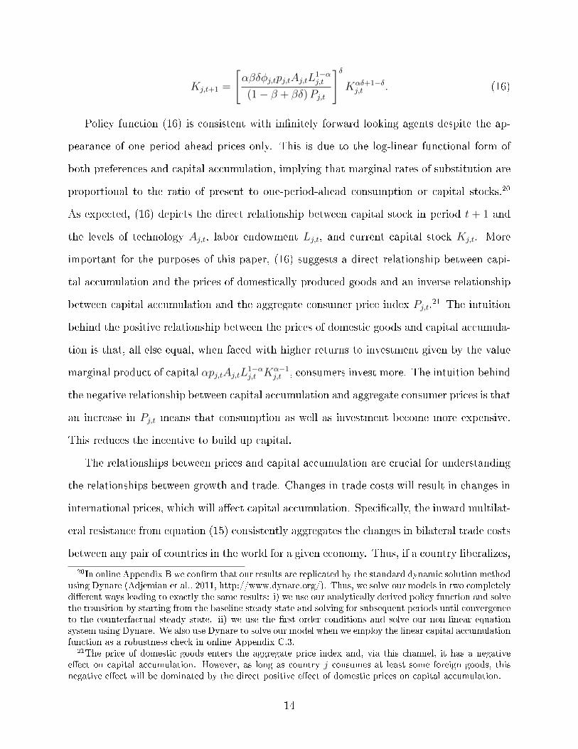
]δKαδ+1−δj,t . (16)

Policy function (16) is consistent with innitely forward looking agents despite the ap-

pearance of one period ahead prices only. This is due to the log-linear functional form of

both preferences and capital accumulation, implying that marginal rates of substitution are

proportional to the ratio of present to one-period-ahead consumption or capital stocks.20

As expected, (16) depicts the direct relationship between capital stock in period t + 1 and

the levels of technology Aj,t, labor endowment Lj,t, and current capital stock Kj,t. More

important for the purposes of this paper, (16) suggests a direct relationship between capi-

tal accumulation and the prices of domestically produced goods and an inverse relationship

between capital accumulation and the aggregate consumer price index Pj,t.21 The intuition

behind the positive relationship between the prices of domestic goods and capital accumula-

tion is that, all else equal, when faced with higher returns to investment given by the value

marginal product of capital αpj,tAj,tL1−αj,t Kα−1

j,t , consumers invest more. The intuition behind

the negative relationship between capital accumulation and aggregate consumer prices is that

an increase in Pj,t means that consumption as well as investment become more expensive.

This reduces the incentive to build up capital.

The relationships between prices and capital accumulation are crucial for understanding

the relationships between growth and trade. Changes in trade costs will result in changes in

international prices, which will aect capital accumulation. Specically, the inward multilat-

eral resistance from equation (15) consistently aggregates the changes in bilateral trade costs

between any pair of countries in the world for a given economy. Thus, if a country liberalizes,

20In online Appendix B we conrm that our results are replicated by the standard dynamic solution methodusing Dynare (Adjemian et al., 2011, http://www.dynare.org/). Thus, we solve our models in two completelydierent ways leading to exactly the same results: i) we use our analytically derived policy function and solvethe transition by starting from the baseline steady state and solving for subsequent periods until convergenceto the counterfactual steady state. ii) we use the rst order conditions and solve our non-linear equationsystem using Dynare. We also use Dynare to solve our model when we employ the linear capital accumulationfunction as a robustness check in online Appendix C.3.

21The price of domestic goods enters the aggregate price index and, via this channel, it has a negativeeect on capital accumulation. However, as long as country j consumes at least some foreign goods, thisnegative eect will be dominated by the direct positive eect of domestic prices on capital accumulation.

14

its inward MR falls and this triggers investment. However, if liberalization takes place in

the rest of the world, this will result in an increase in the MRs for outsiders, and therefore

lower investment. Equation (16) reveals a direct relationship between factory-gate prices and

investment. Similar to the inward MRs, factory-gate prices consistently aggregate the eects

of changes in bilateral trade costs in the world on investment decisions in a given country.

The intuition is that when a country opens to trade, producers in this country enjoy lower

outward MR, which, according to equation (13), translates into higher factory-gate prices.

Outsiders face higher outward MR, their factory-gate prices fall, and investment falls.

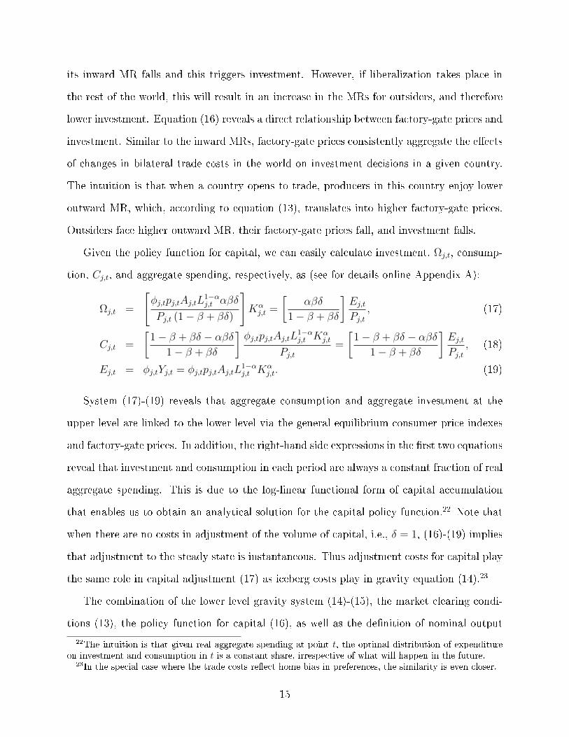
Given the policy function for capital, we can easily calculate investment, Ωj,t, consump-

tion, Cj,t, and aggregate spending, respectively, as (see for details online Appendix A):

Ωj,t =

[φj,tpj,tAj,tL

1−αj,t αβδ

Pj,t (1− β + βδ)

]Kαj,t =

[αβδ

1− β + βδ

]Ej,tPj,t

, (17)

Cj,t =

[1− β + βδ − αβδ

1− β + βδ

]φj,tpj,tAj,tL

1−αj,t Kα

j,t

Pj,t=

[1− β + βδ − αβδ

1− β + βδ

]Ej,tPj,t

, (18)

Ej,t = φj,tYj,t = φj,tpj,tAj,tL1−αj,t Kα

j,t. (19)

System (17)-(19) reveals that aggregate consumption and aggregate investment at the

upper level are linked to the lower level via the general equilibrium consumer price indexes

and factory-gate prices. In addition, the right-hand side expressions in the rst two equations

reveal that investment and consumption in each period are always a constant fraction of real

aggregate spending. This is due to the log-linear functional form of capital accumulation

that enables us to obtain an analytical solution for the capital policy function.22 Note that

when there are no costs in adjustment of the volume of capital, i.e., δ = 1, (16)-(19) implies

that adjustment to the steady state is instantaneous. Thus adjustment costs for capital play

the same role in capital adjustment (17) as iceberg costs play in gravity equation (14).23

The combination of the lower level gravity system (14)-(15), the market clearing condi-

tions (13), the policy function for capital (16), as well as the denition of nominal output

22The intuition is that given real aggregate spending at point t, the optimal distribution of expenditureon investment and consumption in t is a constant share, irrespective of what will happen in the future.

23In the special case where the trade costs reect home bias in preferences, the similarity is even closer.

15

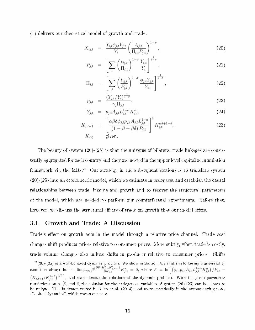
(1) delivers our theoretical model of growth and trade:

Xij,t =Yi,tφj,tYj,t

Yt

(tij,t

Πi,tPj,t

)1−σ

, (20)

Pj,t =

[∑i

(tij,tΠi,t

)1−σYi,tYt

] 11−σ

, (21)

Πi,t =

[∑j

(tij,tPj,t

)1−σφj,tYj,tYt

] 11−σ

, (22)

pj,t =(Yj,t/Yt)

11−σ

γjΠj,t

, (23)

Yj,t = pj,tAj,tL1−αj,t Kα

j,t, (24)

Kj,t+1 =

[αβδφj,tpj,tAj,tL

1−αj,t

(1− β + βδ)Pj,t

]δKαδ+1−δj,t , (25)

Kj,0 given.

The beauty of system (20)-(25) is that the universe of bilateral trade linkages are consis-

tently aggregated for each country and they are nested in the upper level capital accumulation

framework via the MRs.24 Our strategy in the subsequent sections is to translate system

(20)-(25) into an econometric model, which we estimate in order test and establish the causal

relationships between trade, income and growth and to recover the structural parameters

of the model, which are needed to perform our counterfactual experiments. Before that,

however, we discuss the structural eects of trade on growth that our model oers.

3.1 Growth and Trade: A Discussion

Trade's eect on growth acts in the model through a relative price channel. Trade cost

changes shift producer prices relative to consumer prices. More subtly, when trade is costly,

trade volume changes also induce shifts in producer relative to consumer prices. Shifts

24(20)-(25) is a well-behaved dynamic problem. We show in Section A.2 that the following transversality

condition always holds: limt→∞ βt∂F (K∗

j,t,K∗j,t+1)

∂Kj,tK∗j,t = 0, where F ≡ ln

[ (φj,tpj,tAj,tL

1−αj,t Kα

j,t

)/Pj,t −(

Kj,t+1/K1−δj,t

)1/δ ], and stars denote the solutions of the dynamic problem. With the given parameter

restrictions on α, β, and δ, the solution for the endogenous variables of system (20)-(25) can be shown tobe unique. This is demonstrated in Allen et al. (2014), and more specically in the accompanying note,Capital Dynamics, which covers our case.

16

in relative prices aect accumulation, and accumulation aects next period trade. Higher

producer prices increase accumulation because they imply higher returns to investment.

Higher investment and consumer prices, in contrast, reduce accumulation due to higher costs

of investment and due to higher opportunity costs of consumption. Importantly, due to the

general equilibrium forces in our model, changes in trade costs or trade volumes between any

two trading partners potentially aect producer prices and consumer prices in any nation in

the world. In the empirical results, such third-party eects are signicant.

Growth aects trade via two channels, direct and indirect. The direct eect of growth on

trade is strictly positive, acting through country size. Growth in one economy results in more

exports and in more imports with all of its trading partners. The indirect eect of growth

on trade arises because changes in country size translate into changes in the multilateral

resistance for all countries, with knock on changes in trade ows. Importantly, the indirect

channel through which growth aects trade is also a general equilibrium one, i.e., growth

in one country aects trade costs and impacts welfare in every other country in the world.

Work done on other data (e.g. Anderson and Yotov, 2010; Anderson and van Wincoop, 2003)

reveals that a higher income is strongly associated with lower sellers' incidence of trade costs

and thus a real income increase, a correlation replicated here. Closing the loop, growth-led

changes in the incidence of trade costs leads to additional changes in capital stock.

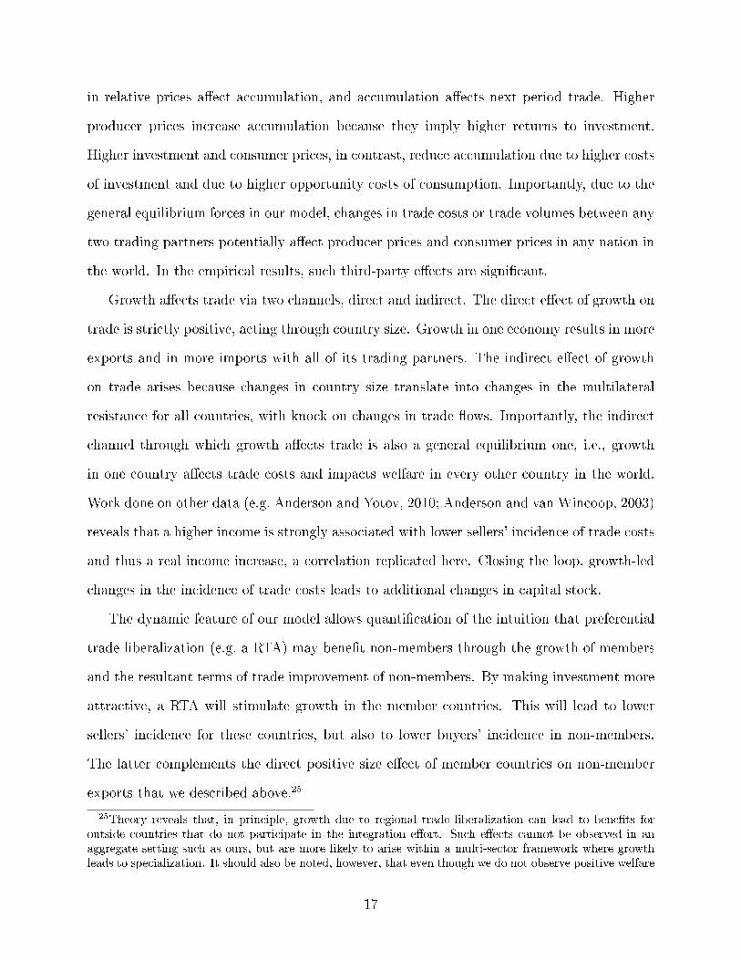
The dynamic feature of our model allows quantication of the intuition that preferential

trade liberalization (e.g. a RTA) may benet non-members through the growth of members

and the resultant terms of trade improvement of non-members. By making investment more

attractive, a RTA will stimulate growth in the member countries. This will lead to lower

sellers' incidence for these countries, but also to lower buyers' incidence in non-members.

The latter complements the direct positive size eect of member countries on non-member

exports that we described above.25

25Theory reveals that, in principle, growth due to regional trade liberalization can lead to benets foroutside countries that do not participate in the integration eort. Such eects cannot be observed in anaggregate setting such as ours, but are more likely to arise within a multi-sector framework where growthleads to specialization. It should also be noted, however, that even though we do not observe positive welfare

17

The long-run eects of trade costs on growth are captured by the comparative statics of

the steady states. Steady-state capital is Kj = Ωj = (αβδφjYj)/[(1− β + βδ)Pj]. The ratio

of steady-state capital stocks between the counterfactual steady state, Kcj , and the baseline

steady state, Kbj , can be expressed as (see online Appendix D for a detailed derivation): Kj =

Kcj/K

bj = P

−σσ(1−α)+αj Π

1−σσ(1−α)+αj Y

1σ(1−α)+α . This expression is intuitive. First, if Pj increases,

capital accumulation becomes more expensive and investment decreases, because Pj captures

the price of investment as well as consumption. Second, increases in sellers' incidence Πj

reduce capital accumulation because Πj aects pj inversely, so the value marginal product

of capital falls with Πj, decreasing the incentive to invest. Third, as the world gets richer,

measured by an increase of world GDP (Y ), capital accumulation in j increases to eciently

serve the larger world market.

In a recent inuential paper, ACR demonstrate that the welfare eects of trade liberaliza-

tion in a wide range of trade models can be summarized by the following sucient statistics:

Wj = λ1

1−σjj , where λjj denotes the share of domestic expenditure and hat denotes the ratio

of the counterfactual and baseline value. Motivated by ACR, we show (in online Appendix E)

that the change in capital can directly aect welfare by deriving an extended ACR formula:

Wj = Kαj λ

11−σjj . (26)

Equation (26) implies that an increase of steady-state capital will, ceteris paribus, in-

crease welfare. The extended ACR formula given in (26) holds in and out-of steady state.

Furthermore, as demonstrated in online Appendix E, we can express Kj in terms of λjj in

steady state, leading to Wj = λ1

(1−α)(1−σ)jj . This expression nicely highlights the similarity of

introducing capital or intermediates in the steady state (compare with ACR, p. 115).

We are also able to derive an ACR-like welfare formula, which only depends on λjj,t and

parameters when taking into account the transition (see online Appendix E.2). However,

we will typically not observe changes in λjj,t over time solely driven by the counterfactual

eects for outside countries in our sample, we do nd non-monotonic trade diversion eects. In some cases(e.g. Austria), the dynamic forces in our framework lead to trade creation eects that are stronger than theinitial static trade diversion eects. Details are available in Table A4 of online Appendix J.

18

under consideration. While the standard approach in a static setting is to measure welfare in

terms of real GDP, our dynamic capital-accumulation framework requires some adjustments

to this standard approach for the following reasons: (i) Transition between steady states

is not immediate due to the gradual adjustment of capital stocks. Given our upper level

equilibrium, we are able to solve the transition path for capital accumulation simultaneously

in each of the N -countries in our sample.26 (ii) Consumers in our setting divide their income

between consumption and investment. Thus, only part of GDP is used to derive utility. In

order to account for these features of our model, we follow Lucas (1987) and calculate the

constant fraction ζ of aggregate consumption in each year that consumers would need to be

paid in the baseline case to give them the same utility they obtain from the consumption

stream in the counterfactual (Ccj,t). Specically, we calculate:

∞∑t=0

βt ln(Ccj,t

)=

∞∑t=0

βt ln

[(1 +

ζ

100

)Cbj,t

]⇒

ζ =

(exp

[(1− β)

( ∞∑t=0

βt ln(Ccj,t

)−

∞∑t=0

βt ln(Cbj,t

))]− 1

)× 100. (27)

4 Empirical Analysis

Our model is straightforward to implement empirically. It simultaneously enables us to

test and establish the causal relationships between trade, income, and growth, and it also

delivers all the key parameters needed to perform counterfactuals. The parameter estimates

that we obtain are compared to standard values from the existing literature to establish the

credibility of our methods. The econometric framework includes as a special case the reduced-

form income-and-trade specication from Frankel and Romer (1999), but also expands on

it by proposing a novel instrument for trade openness and by introducing an additional

estimating equation for capital accumulation while highlighting important contributions of

26Given our closed-form solution of the policy function for capital and an initial capital stock Kj,0, thisboils down to solving system (20)-(25) for all countries at each point of time. Alternatively, we used Dynare(http://www.dynare.org/) and the implied rst-order conditions of our dynamic system to solve the transitionpath. Both lead to identical results. For further computational details see online Appendix B.

19

our structural approach. Section 4.1 presents the estimation strategy and some econometric

challenges. Section 4.2 describes the data and Section 4.3 presents the estimates.

4.1 Econometric Specication

We translate our theoretical model into estimating equations in two steps. We begin with the

estimation strategy for the lower level, the gravity model of trade ows. Then, we describe

the estimation strategy for the upper level equations for income and for capital.

4.1.1 Lower Level Econometric Specication: Trade

To obtain sound econometric estimates of bilateral trade costs and, subsequently, of the

multilateral resistances that enter the income and capital equations, several econometric

challenges must be met. First, we follow Santos Silva and Tenreyro (2006) in the use of

the Poisson Pseudo-Maximum-Likelihood (PPML) estimator to account for the presence of

heteroskedasticity and zeros in trade data. Second, we use time-varying, directional (exporter

and importer), country-specic xed eects to account for the unobservable multilateral

resistances. Importantly, in addition to controlling for the multilateral resistances, the xed

eects in our econometric specication also absorb national output and expenditure and,

therefore, control for all dynamic forces from our theory. Third, to avoid the critique from

Cheng and Wall (2005) that [f]ixed-eects estimation is sometimes criticized when applied to

data pooled over consecutive years on the grounds that dependent and independent variables

cannot fully adjust in a single year's time. (footnote 8, p. 52), we use 3-year intervals.27

The nal step, which completes the econometric specication of our trade system, is to

provide structure behind the unobservable bilateral trade costs tij,t. We employ a exible

country-pair xed eects approach in order to account for all (observable and unobservable)

time-invariant trade costs. In addition, we use RTAs to capture the eects of trade policy.28

27Treer (2004) also criticizes trade estimations pooled over consecutive years. He uses three-year intervals.Baier and Bergstrand (2007) use 5-year intervals. Olivero and Yotov (2012) provide empirical evidence thatgravity estimates obtained with 3-year and 5-year lags are very similar, but the yearly estimates producesuspicious trade cost parameters. Here, we use 3-year intervals in order to improve eciency, but we alsoexperiment with 4- and 5-year lags to obtain qualitatively identical and quantitatively very similar results.

28We chose to focus exclusively on RTAs in order emphasize the methodological contributions of our work.

20

Econometrically, we have to address the potential endogeneity of RTAs. The issue of RTA

endogeneity is well-known in the trade literature29 and to address it, we adopt the method

from Baier and Bergstrand (2007) and use country-pair xed eects in order to account for

the unobservable linkages between the RTAs and the error term in our trade regressions.

Taking all of the above considerations into account, we employ PPML to estimate the

following econometric specication of the Trade equation (20) from our structural system:

Xij,t = exp[η1RTAij,t + χi,t + πj,t + µij] + εij,t, (28)

where RTAij,t is a dummy variable equal to 1 when i and j have a RTA in place at time

t, and zero elsewhere. χi,t denotes the time-varying source-country dummies, which control

for the outward multilateral resistances and countries' output shares. πj,t encompasses the

time varying destination country dummy variables that account for the inward multilateral

resistances and total expenditure. µij denotes the set of country-pair xed eects that should

absorb the linkages between RTAij,t and the remainder error term εij,t in order to control for

potential endogeneity of the former. Importantly, µij will absorb all time-invariant gravity

covariates, such as bilateral distance, contiguous borders, common language and colonial ties,

along with any other time-invariant determinants of trade costs that are not observable. We

use the estimates of the country-pair xed eects µij from equation (28) to measure directly

international trade costs in the absence of RTAs (for details please see online Appendix F):(tNORTAij

)1−σ= exp [µij] . (29)

In principle, we also may introduce taris and other time-varying trade costs in the estimating gravityequation (28). However, bringing tari revenues fully into the model opens Pandora's Box, because muchof their distortionary eect (and much of the diculty of negotiating regional trade agreements) is due todispersion of rates across sectors within countries. Moreover, a proper treatment of eects of trade agreementsvia government revenue should in principle include eects on domestic distortionary tax collections, eectslikely to be much larger (because tax rates are higher) than those from trade tax revenues. We refer theinterested reader to Anderson and van Wincoop (2001) and to Egger et al. (2011) for modeling and empiricalinvestigation of the role of heterogeneous tari revenues in gravity models. Instead, here we choose to abstractfrom modeling such time-varying trade costs and potential tari revenues and rents in order to be able toclearly isolate the pure dynamic eects of a single one-time trade shock, such as the introduction or theremoval of an RTA, which will enable us to focus on and emphasize our methodological contributions.

29See for example Treer (1993), Magee (2003) and Baier and Bergstrand (2002, 2004).

21

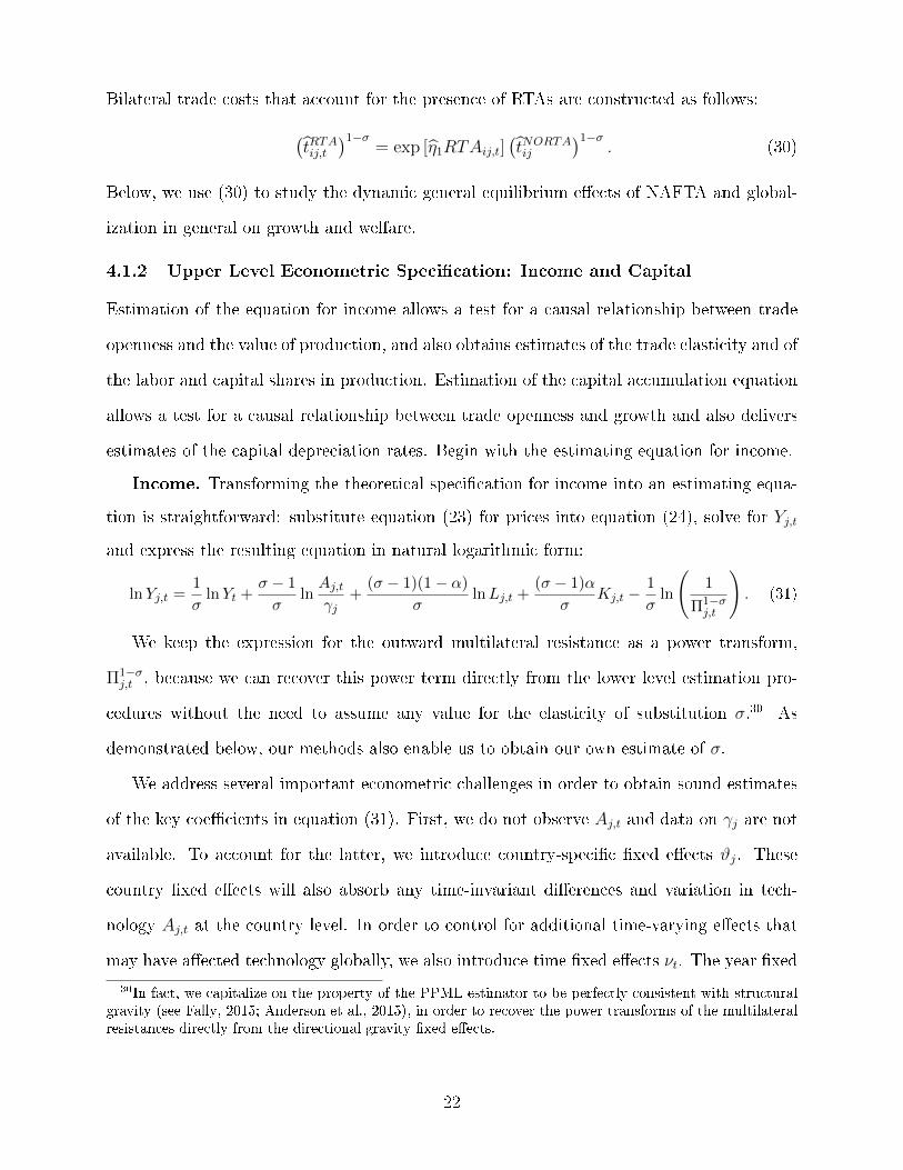
Bilateral trade costs that account for the presence of RTAs are constructed as follows:

(tRTAij,t

)1−σ= exp [η1RTAij,t]

(tNORTAij

)1−σ. (30)

Below, we use (30) to study the dynamic general equilibrium eects of NAFTA and global-

ization in general on growth and welfare.

4.1.2 Upper Level Econometric Specication: Income and Capital

Estimation of the equation for income allows a test for a causal relationship between trade

openness and the value of production, and also obtains estimates of the trade elasticity and of

the labor and capital shares in production. Estimation of the capital accumulation equation

allows a test for a causal relationship between trade openness and growth and also delivers

estimates of the capital depreciation rates. Begin with the estimating equation for income.

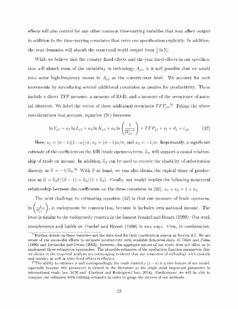
Income. Transforming the theoretical specication for income into an estimating equa-

tion is straightforward: substitute equation (23) for prices into equation (24), solve for Yj,t

and express the resulting equation in natural logarithmic form:

lnYj,t =1

σlnYt +

σ − 1

σlnAj,tγj

+(σ − 1)(1− α)

σlnLj,t +

(σ − 1)α

σKj,t −

1

σln

(1

Π1−σj,t

). (31)

We keep the expression for the outward multilateral resistance as a power transform,

Π1−σj,t , because we can recover this power term directly from the lower level estimation pro-

cedures without the need to assume any value for the elasticity of substitution σ.30 As

demonstrated below, our methods also enable us to obtain our own estimate of σ.

We address several important econometric challenges in order to obtain sound estimates

of the key coecients in equation (31). First, we do not observe Aj,t and data on γj are not

available. To account for the latter, we introduce country-specic xed eects ϑj. These

country xed eects will also absorb any time-invariant dierences and variation in tech-

nology Aj,t at the country level. In order to control for additional time-varying eects that

may have aected technology globally, we also introduce time xed eects νt. The year xed

30In fact, we capitalize on the property of the PPML estimator to be perfectly consistent with structuralgravity (see Fally, 2015; Anderson et al., 2015), in order to recover the power transforms of the multilateralresistances directly from the directional gravity xed eects.

22

eects will also control for any other common time-varying variables that may aect output

in addition to the time-varying covariates that enter our specication explicitly. In addition,

the year dummies will absorb the structural world output term 1σ

lnYt.

While we believe that the country xed eects and the year xed eects in our specica-

tion will absorb most of the variability in technology Aj,t, it is still possible that we would

miss some high-frequency moves in Aj,t at the country-year level. We account for such

movements by introducing several additional covariates as proxies for productivity. These

include a direct TFP measure, a measure of R&D, and a measure of the occurrence of natu-

ral disasters. We label the vector of these additional covariates TFPj,t.31 Taking the above

considerations into account, equation (31) becomes:

lnYj,t = κ1 lnLj,t + κ2 lnKj,t + κ3 ln

(1

Π1−σj,t

)+ TFPj,t + νt + ϑj + εj,t. (32)

Here, κ1 = (σ−1)(1−α)/σ, κ2 = (σ−1)α/σ, and κ3 = −1/σ. Importantly, a signicant

estimate of the coecient on the MR/trade openness term, κ3, will support a causal relation-

ship of trade on income. In addition, κ3 can be used to recover the elasticity of substitution

directly as σ = −1/κ3.32 With σ at hand, we can also obtain the capital share of produc-

tion as α = κ2σ/(σ − 1) = κ2/(1 + κ3). Finally, our model implies the following structural

relationship between the coecients on the three covariates in (32), κ1 + κ2 = 1 + κ3.

The next challenge to estimating equation (32) is that our measure of trade openness,

ln

(1

Π1−σj,t

), is endogenous by construction, because it includes own national income. The

issue is similar to the endogeneity concern in the famous Frankel and Romer (1999). Our work

complements and builds on Frankel and Romer (1999) in two ways. First, in combination,

31Further details on these variables and the data used for their construction appear in Section 4.2. We areaware of the successful eorts to estimate productivity with available rm-level data, cf. Olley and Pakes(1996) and Levinsohn and Petrin (2003). However, the aggregate nature of our study does not allow us toimplement those estimation approaches. The plausible estimates of the production function parameters thatwe obtain in the empirical analysis are encouraging evidence that our treatment of technology with controlsand country as well as time xed eects is eective.

32The ability to estimate σ and correspondingly the trade elasticity (1− σ) is a nice feature of our model,especially because this parameter is viewed in the literature as the single most important parameter ininternational trade (see ACR and Costinot and Rodríguez-Clare, 2014). Furthermore, we will be able tocompare our estimates with existing estimates in order to gauge the success of our methods.

23

equations (28) and (32) deliver a structural foundation for the reduced-form trade-and-

income specication from Frankel and Romer (1999). Frankel and Romer use a version of

Trade equation (28) to instrument for international trade, which enters their Income equation

corresponding to equation (32) directly, to replace our structural term ln(1/Π1−σ

j,t

). Instead,

in our specication, the eects of trade and trade openness on income are channeled via the

structural trade term ln(1/Π1−σ

j,t

). Importantly, this will enable us not only to test for a

causal relationship between trade openness and income, but also to recover an estimate for

the elasticity of substitution σ = −1/κ3.33

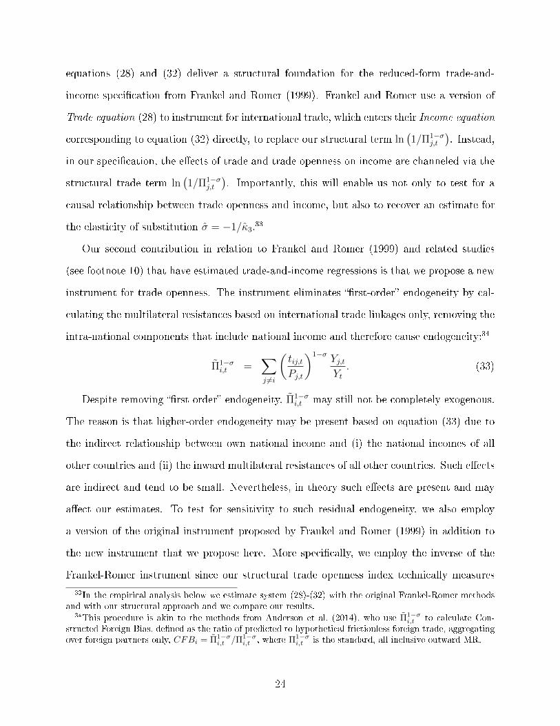
Our second contribution in relation to Frankel and Romer (1999) and related studies

(see footnote 10) that have estimated trade-and-income regressions is that we propose a new

instrument for trade openness. The instrument eliminates rst-order endogeneity by cal-

culating the multilateral resistances based on international trade linkages only, removing the

intra-national components that include national income and therefore cause endogeneity:34

Π1−σi,t =

∑j 6=i

(tij,tPj,t

)1−σYj,tYt. (33)

Despite removing rst-order endogeneity, Π1−σi,t may still not be completely exogenous.

The reason is that higher-order endogeneity may be present based on equation (33) due to

the indirect relationship between own national income and (i) the national incomes of all

other countries and (ii) the inward multilateral resistances of all other countries. Such eects

are indirect and tend to be small. Nevertheless, in theory such eects are present and may

aect our estimates. To test for sensitivity to such residual endogeneity, we also employ

a version of the original instrument proposed by Frankel and Romer (1999) in addition to

the new instrument that we propose here. More specically, we employ the inverse of the

Frankel-Romer instrument since our structural trade openness index technically measures

33In the empirical analysis below we estimate system (28)-(32) with the original Frankel-Romer methodsand with our structural approach and we compare our results.

34This procedure is akin to the methods from Anderson et al. (2014), who use Π1−σi,t to calculate Con-

structed Foreign Bias, dened as the ratio of predicted to hypothetical frictionless foreign trade, aggregatingover foreign partners only, CFBi = Π1−σ

i,t /Π1−σi,t , where Π1−σ

i,t is the standard, all-inclusive outward MR.

24

the inverse of trade openness. We oer further details on these instruments in Section 4.3.

The nal challenge with the estimation of Specication (32) is that the labor and capital

covariates are potentially endogenous as well. In Section 4.3 we account for these endogeneity

concerns sequentially and we also treat all regressors from specication (32) simultaneously

as endogenous by using a series of instruments that pass all relevant econometric IV tests.

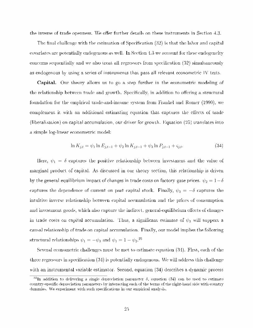
Capital. Our theory allows us to go a step further in the econometric modeling of

the relationship between trade and growth. Specically, in addition to oering a structural

foundation for the empirical trade-and-income system from Frankel and Romer (1999), we

complement it with an additional estimating equation that captures the eects of trade

(liberalization) on capital accumulation, our driver for growth. Equation (25) translates into

a simple log-linear econometric model:

lnKj,t = ψ1 lnEj,t−1 + ψ2 lnKj,t−1 + ψ3 lnPj,t−1 + ςj,t. (34)

Here, ψ1 = δ captures the positive relationship between investment and the value of

marginal product of capital. As discussed in our theory section, this relationship is driven

by the general-equilibrium impact of changes in trade costs on factory-gate prices. ψ2 = 1−δ

captures the dependence of current on past capital stock. Finally, ψ3 = −δ captures the

intuitive inverse relationship between capital accumulation and the prices of consumption

and investment goods, which also capture the indirect, general-equilibrium eects of changes

in trade costs on capital accumulation. Thus, a signicant estimate of ψ3 will support a

causal relationship of trade on capital accumulation. Finally, our model implies the following

structural relationships ψ1 = −ψ3 and ψ1 = 1− ψ2.35

Several econometric challenges must be met to estimate equation (34). First, each of the

three regressors in specication (34) is potentially endogenous. We will address this challenge

with an instrumental variable estimator. Second, equation (34) describes a dynamic process

35In addition to delivering a single depreciation parameter δ, equation (34) can be used to estimatecountry-specic depreciation parameters by interacting each of the terms of the right-hand side with countrydummies. We experiment with such specications in our empirical analysis.

25

where capital stock in the current period is a function of capital stock in past periods,

i.e., the dependent variable is determined by its past realizations. As discussed in detail in

Roodman (2009), this gives rise to dynamic panel bias since the dependent variable is clearly

correlated with the xed eects in the error term. A straightforward approach to mitigate

the dynamic panel bias is to explicitly control for the country xed eects in our panel with

the Least Squares Dummy Variables (LSDV) estimator. Specically, we add to equation (34)

country xed eects (ϑj) and year xed eects (νt) in order to control for any unobserved

and omitted time-varying global eects that may aect capital accumulation. Additionally,

νt and ϑj control for variation in the parameters δ ln [(αβδ)/(1− β + βδ)]. In combination

with the year dummies, the country xed eects will not only mitigate the dynamic bias

but also will control for any time-invariant country-specic characteristics that may aect

capital accumulation but are omitted from our model, thus alleviating endogeneity concerns.

The rich set of xed eects may not fully absorb all possible causes for endogeneity.

Furthermore, the country xed eects do not completely absorb the correlation between the

dependent variable and the dynamic error term and our estimates are still subject to the

Nickell (1981) dynamic bias. In order to address these concerns we use a series of instrumental

variables and we employ the Arellano and Bond (1991) linear generalized method of moments

(GMM) estimator. Further details on our empirical strategy are presented in Section 4.3.

In combination, equations (28), (32), and (34), deliver the econometric version of our

structural system of growth and trade. With these three estimating equations we obtain

estimates of the key parameters needed to calibrate our model of trade and growth. In

addition, the system will enable us to isolate and identify the causal eect of trade on

income and growth via the estimates of κ3 and ψ3 on the trade terms ln

(1

Π1−σj,t

)and lnPj,t−1

in our Income equation (32) and Capital equation (34), respectively. We demonstrate below.

Before that we describe our data.

26

4.2 Data

Our sample covers 82 countries over the period 1990-2011.36 These countries account for

more than 98 percent of world GDP during that period. The data include trade ows,

GDP, employment, capital and RTAs. Bilateral trade cost proxies are data on standard

gravity variables including distance, common language, contiguity and colonial ties along

with regional trade agreements in eect.

Data on GDP, employment, capital stocks, and total factor productivity (TFP) are from

the Penn World Tables 8.0.37 The Penn World Tables 8.0 oer several GDP variables.

Following the recommendation of the data developers, we employ Output-side real GDP

at current PPPs (CGDP o), which compares relative productive capacity across countries

at a single point in time, as the initial level in our counterfactual experiments, and we

use Real GDP using national-accounts growth rates (CGDP na) for our output-based cross-

country income regressions. The Penn World Tables 8.0 include data that enables us to

measure employment in eective units. To do this we multiply the Number of persons

engaged in the labor force with the Human capital index, which is based on average years of

schooling. Capital stocks (at constant 2005 national prices in mil. 2005USD) in the Penn

World Tables 8.0 are constructed based on cumulating and depreciating past investment

using the perpetual inventory method. As a main measure for total factor productivity we

use TFP level at current PPPs. For more detailed information on the construction and the

original sources for the Penn World Tables 8.0 series see Feenstra et al. (2013). In addition,

we also employ a measure for research and development (R&D) spending, which is taken

from the World Development Indicators. Finally, we experiment with an instrument for

occurrence of natural disasters, which comes from EM-DAT - The International Disaster

Database.38

Aggregate trade data come from the United Nations Statistical Division (UNSD) Com-

36The list of countries and their respective labels can be found in online Appendix G.37These series are now maintained by the Groningen Growth and Development Centre and reside at

http://www.rug.nl/research/ggdc/data/pwt/.38http://www.emdat.be/database.

27

modity Trade Statistics Database (COMTRADE). The trade data in our sample includes

only 5.8 percent of zeroes due to its aggregate nature. The RTA-dummy is constructed based

on information from the World Trade Organization. A detailed description of the RTA data

used and the data set itself can be found at http://www.ewf.uni-bayreuth.de/en/research/

RTA-data/index.html. Finally, data on the standard gravity variables, i.e., distance, com-

mon language, colonial ties, etc., are from the CEPII's Distances Database.

4.3 Estimation Results and Analysis

4.3.1 Trade Costs

Specication (28) delivers an estimate of the average treatment eect of RTAs that is equal

to 0.827 (std.err. 0.135), which is readily comparable to the corresponding index of 0.76

from Baier and Bergstrand (2007).39 This gives us condence to use our estimate of the

RTA eects to proxy for the eects of trade liberalization in the counterfactual experiments.

Without going into details, we briey discuss several properties of the bilateral trade

costs, which are constructed as tij = exp(µij)1/(1−σ), where we use a conventional value of

the elasticity of substitution, σ = 6 (see for details online Appendix F).40 All estimates of

tij are positive and greater than one. The mean estimate of bilateral trade costs is 5.569

(std.dev. 4.216). Estimates of the bilateral xed eects vary widely but intuitively across

the country pairs in our sample. For example, we obtain the lowest estimates of tij for

countries that are geographically and culturally close and economically integrated. The

smallest estimate of bilateral trade costs is for the pair Malaysia-Singapore (1.184), followed

by Belgium-Netherlands (1.327). While more than 95% of our estimates of bilateral trade

costs are smaller than 12, we also obtain some very large estimates of tij for countries that

are isolated economically and geographically. The largest estimate is for the pair Uzbekistan-

39Our RTA estimate suggest a partial equilibrium increase of 129% (100 × [exp(0.827) − 1]) in bilateraltrade ows among member countries.

40Head and Mayer (2014) survey the related literature and report average values and standard deviationsof 744 elasticity estimates obtained from a sample of 32 papers. The mean estimate of σ from Head andMayer (2014) when the selection criteria is structural gravity estimation, as in our analysis, is σ = 6.13.Importantly, below we obtain our own structural estimate of σ = 5.847 (std.err. 0.620), which is remarkablyclose to (and, in fact, not statistically dierent from) Head and Mayer's index.

28

Dominican Republic (132.7). Most other pairs with very large bilateral trade cost estimates

also include as one partner one of the less developed former Soviet republics. This result is

consistent with the ndings of Waugh (2010) that trade ows in less developed countries are

subject to larger trade costs. Another outlier pair is Israel-Iran (30.21). We note that these

estimates are obtained directly from the pair xed eects as a very exible proxy for trade

costs. This suggests that the standard set of proxies for trade costs that are routinely used

in gravity estimations may miss to account for some important obstacles to international

trade, especially among less developed pairs.

4.3.2 Income

Estimates from various specications of Income equation (32) are reported in Table 1. All

specications include year xed eects and country xed eects, and we report standard

errors that are robust or bootstrapped when a generated regressor enters the estimating

equation directly. We begin with two benchmark specications. In columns (1) and (2)

of Table 1, respectively, we oer results from an unconstrained and from a constrained

estimation of a standard Cobb-Douglas production function. As can be seen from the table,

both the labor and the capital shares in each specication are within the theoretical bounds

[0; 1] even though the capital share is a bit higher than the standard corresponding value

from the literature.41

Column (3) of Table 1 reports estimates of a Frankel-Romer type specication, where

we introduce the log of international trade/total exports, ln∑

j 6=iXij,t, as an additional

regressor in the unconstrained Cobb-Douglas estimation from column (1). As correctly

noted by Frankel and Romer (1999), the trade regressor is endogenous. Therefore, we follow

Frankel and Romer's strategy and perform an IV estimation, where bilateral exports are

predicted in a rst-stage gravity model by the standard gravity regressors (see for details

online Appendix F) and by the logarithms of exporter and importer populations. Our rst-

stage gravity regression follows the recommendation of Feyrer (2009b) not to use exporter

41Below, we oer some validity checks with respect to the estimated capital share. Moreover, in thesensitivity analysis for our counterfactuals we experiment with alternative values for α.

29

and importer xed eects in a Frankel-Romer setting because the directional xed eects

will contaminate the IV estimation since they implicitly account for income and expenditure.

Results from the IV experiment are presented in column (3) of Table 1. Consistent with

the ndings of Frankel and Romer (1999), our estimates conrm that the eect of trade on

income/growth is positive and statistically signicant. In addition, our instruments pass the

underidentication and the weak identication test that we also report in the bottom of

panel A. Overall, the results from the Frankel-Romer experiment are consistent with those

from the literature.

In columns (4) and (5) of Table 1, we replace the trade variable from the reduced-form

Frankel-Romer specication with our structural trade openness measure. The estimates in

column (4) are unconstrained, while the specication in column (5) imposes the structural

restrictions of our theory. The constrained and the unconstrained results are very similar,

and not statistically dierent from each other. This is encouraging preliminary evidence in

support of our model. It also enables us to focus interpretation on the constrained estimates

from column (5), where we see that estimates have expected signs and are statistically

signicant at any conventional level. Importantly, we nd that trade openness leads to

higher income. This is captured by the negative and signicant estimate of the coecient

of our inverse theoretical measure of trade openness ln(

1/Π1−σj,t

). Thus, our model and

estimates oer evidence for a causal relationship between trade and income.

The structural properties of the model yield estimates of the elasticity of substitution, σ,

and of the capital share, α, which are reported at the bottom of column (5). The inferred

value of σ = −1/κ3 = 4.084 falls comfortably within the distribution of the existing (Arm-

ington) elasticity numbers from the trade literature, which usually vary between 2 and 12.

(See footnote 16). The inferred estimate of the capital share α = 0.572 is a bit higher than

expected but falls within the theoretically required interval [0;1].

The specication in column (6) addresses potential high-frequency (country-year) tech-

nology changes not controlled for with the set of country and year xed eects in the econo-

30

metric model. We introduce a direct TFP measure as a covariate, taken from the Penn World

Tables. We obtain a positive and signicant estimate on the coecient of TFPj,t. The addi-

tion of the TFP measure does not aect our ndings qualitatively, as all estimates are still

statistically signicant at any level and with signs as expected. However, the magnitudes

of the eects of labor, capital, and trade openness are changed. Specically, controlling for

TFP decreases the eects of eective labor and trade openness and leads to a higher esti-

mate of the eect of capital. The reduction in importance of trade openness is attributable

to the fact that multilateral resistance is part of TFP. The structural estimate of the elas-

ticity of substitution increases to σ = −1/κ3 = 10.114, which is now on the higher end of

the distribution of corresponding estimates from the literature. In online Appendix C.1 we

also add R&D and the occurrence of natural disasters as possible candidates that may aect

productivity and income. None of the eects of these variables is signicant and they do not

aect the estimates of the eects of the other covariates in our specication. We capitalize

on this result below, where we use the occurrence of natural disasters as an instrument in

the IV specications of our Income equation.

We account for endogeneity of trade openness in columns (7) and (8) of Table 1. First, in

column (7), we use the new structural instrument that we proposed in Section 4.1.2, which

is constructed after explicitly removing the endogenous components from the OMR/trade

openness index. In addition, we also employ the lag of our openness regressor in order to

mitigate simultaneity concerns. The IV results in column (7) are encouraging. All variables

retain their signs and statistical signicance. In addition, as evident from the test statistics

reported at the bottom of panel A, our instruments pass the underidentication, the weak

identication, and also the overidentication tests. Inspection of the rst stage IV estimates

reveals that both of our instruments are highly statistically signicant and contribute signif-

icantly to explain the variability in the endogenous trade openness regressor. The estimates

from panel B reveal that the structural parameters that we recover are also within the the-

oretical limits and are comparable to the estimates from column (6). In sum, our results

31

suggest that the new instrument proposed here performs well. Nevertheless, in column (8) of

Table 1, we also add the inverse of the Frankel-Romer instrument that we used to obtain the

results from column (3). As noted earlier, we use the inverse of this instrument because our

structural trade term is an inverse measure of trade openness by construction. The estimates

in column (8) are virtually identical to those from column (7). In addition, once again, the

instruments pass all IV tests.

Next, we control for endogenous capital, endogenous labor, and endogenous TFP in

columns (9), (10), and (11), respectively, of Table 1. Our approach is to endogenize one

additional variable at a time while still treating all variables that already have been endo-

genized in previous specications as endogenous. As a result, the estimates in column (11)

are obtained with all covariates from equation (32) being treated as endogenous. In column

(9), we use lagged capital stocks and occurrence of natural disasters to instrument for cur-

rent capital stock. Then, in column (10), we also allow for endogenous labor in addition

to endogenous capital and endogenous trade openness, and we add the log of population

to instrument for labor in addition to the instruments for capital and those for openness.

Finally, in column (11), we add lagged and 2-period lagged TFP as instruments for current

TFP. The estimates from column (11), where trade openness, capital, labor, and TFP are

all treated as endogenous, are very similar to those from column (8), where only trade open-

ness was treated as endogenous. The values of the structural parameters from column (11)

are also similar to the corresponding estimates from column (8). Finally, we note that the

instruments that we use in each of specications (9)-(11) pass all IV tests.

The last column of Table 1 presents our main results, obtained after controlling for en-

dogeneity of all covariates (as in column (11)), while simultaneously imposing the structural

constraints of our model (as in column (5)). Estimates of all covariates have expected signs,

reasonable magnitudes, and are signicant at any conventional level. The structurally esti-

mated capital share is a bit higher than expected, but it is still within the theoretical bounds.

With a value of 5.847, our estimate of elasticity of substitution is right in the middle of the

32

standard range from the literature and it is not statistically dierent from the summary

measure of σ = 6.13 reported in Head and Mayer (2014).42

Overall, the parameter estimates of α and σ that we obtain in this section are plausible.

Furthermore, we view the stable and robust performance of our results across all the speci-

cations in Table 1, which range from a very basic unconstrained OLS model (column (4)) to

a constrained IV specication that allows for all structural terms to be endogenous (column

(12)), as encouraging evidence in support of our model.

4.3.3 Capital

To estimate the capital accumulation equation (34) we use the main estimate of the elasticity

of substitution σ = 5.847 from our income regressions to construct lnPj,t−1 from the power

transform of the inward multilateral resistance.43 Equation (34) will enable us to recover

capital depreciation rates (δ's) subject to the following relationships: ψ1 = δ; ψ2 = 1 − δ;

and ψ3 = −δ. In addition, the estimate of the coecient ψ3 on lnPj,t−1 will enable us to

test our theory for a positive relationship between trade and capital accumulation.

Begin with a simple OLS regression based on (34). Results are presented in column

(1) of Table 2. The estimates of all three covariates are statistically signicant at any

conventional level and with expected signs. The estimate on the lagged capital stock variable

is very close to one and very precisely estimated, capturing strong persistence as expected.

Importantly, the estimate of the coecient on the trade openness term lnPj,t−1 is negative

and statistically signicant, suggesting a positive causal relationship between trade openness

and capital accumulation. The intuition is that, in accordance with our theory, the estimate

42Our estimates reveal that the elasticity of income with respect to the Frankel-Romer measure of openness,which we obtain in column (3), is higher as compared to the elasticity with respect to our structural measureof openness. We oer two possible explanations. First, gravity theory may explain part of the dierences.Specically, we note that our structural measure of trade openness represents only one component of thetheoretically predicted trade variable from Frankel and Romer. Second, we add as a control in the incomeregression a direct TFP measure. Comparison between the results from columns (4) and (5) reveal that,while all of our estimates remain signicant and with expected signs, the introduction of TFP aects themagnitude of our results and they become smaller.

43Results are robust to using alternative values for σ. For example, below we will use our structuralspecication with σ = 5.847 to recover a capital depreciation rate δ = 0.061. This estimate varies between0.054 and 0.063 for corresponding values of σ equal to 3 and 12.

33

of ψ3 captures the inverse relationship between investment and the costs of investment (both

direct and opportunity costs). Finally, we obtain a positive and signicant estimate of the

coecient on the expenditure term lnEj,t−1, which, as suggested by our model, captures the

positive relationship between the value of marginal product of capital and investment.

The estimates in column (2) of Table 2 are obtained from the same specication as in

column (1) under the structural constraints of our model. All estimates are statistically

signicant at any conventional level and have expected signs. The capital depreciation rate

is relatively low at 1.6 percent. Possible reasons for the downward bias in our estimate of the

depreciation include (i) endogenous regressors and (ii) Nickell dynamic panel bias (Nickell,

1981) due to the use of the lagged dependent variable as a regressor in specication (34).

In columns (3), (4), and (5) of Table 2, respectively, we sequentially treat the lags of trade

openness, expenditure, and the stock of capital as endogenous. Our approach is to endogenize

one additional variable at a time while still treating all variables that have been endogenized

in previous specications as endogenous. In column (3), we use two instruments for trade

openness. These instruments include the second lag of the endogenous variable lnPj,t−1 and

the second lag of the openness variable but, as discussed in section 4.1.2, constructed without

intra-national components. In column (4), we instrument for lagged expenditure with the

second lags of this variable and of the variable for occurrence of natural disasters. Finally,

in column (5) we also instrument for the lagged capital stock variable with its second lag.

The results from columns (3)-(5) are similar and in accordance with our ndings from the

simple baseline OLS specication from column (1). In addition, our instruments pass the IV

tests of underidentication, weak identication, and overidentication.

The estimates in column (6) of Table 2 are obtained with the Least Squares Dummy

Variables (LSDV) estimator with country and year xed eects added to specication (34),

while all covariates are still treated as endogenous. As noted in Roodman (2009), this is a

natural rst step to mitigate (but not to eliminate) the dynamic panel bias by purging the

country xed eects out of the error term. The estimates in column (6) are qualitatively

34

identical and quantitatively similar to those from the previous specications. The main

dierence is the increase in the magnitude of the estimate on the lagged value of expenditure.

In addition, we see that the estimates on lagged capital stock and on trade openness are a

bit smaller, the latter still statistically signicant but marginally so. Once again, we note

that the instruments from the LSDV specication pass all IV tests. Finally, we nd that

two of the three structural constrains of our theory are satised in this specication.

Our main estimates of the Capital equation are presented in column (7) of Table 2. To

obtain these results we treat all regressors as endogenous and we use the full set of xed

eects, as in column (6), but under the structural constraints of our model. The eects of all

structural terms are highly signicant and with expected signs. The estimate of the capital

depreciation rate is 6.1 percent, suggesting that the depreciation rate δ = 0.016 from column

(2) was indeed biased due to endogeneity and dynamic panel biases.

Next, we employ the dynamic panel-data estimator proposed by Arellano and Bond

(1991) and rened by Arellano and Bover (1995) and Blundell and Bond (1998) in order to

account for the remaining Nickell bias, which may still be present in our sample even after

the inclusion of the country xed eects because the lagged dependent variable may still be

correlated with the unobserved panel eects within each country group. Since the expendi-

ture and trade openness regressors are also functions of capital, we treat those covariates as

potentially subject to dynamic bias concerns as well. Thus, our set of instruments includes

all lags of all three endogenous regressors. In addition, we add as level instruments our struc-

tural trade openness instrument, the occurrence of natural disasters and the second lags of

the logarithms of capital and expenditure. As in all previous specications, the estimates in

column (8) are obtained with robust standard errors and year and country xed eects.

The results from column (8) of Table 2 reveal that, as in our main specication from

column (7), the estimates of all regressors in the Capital equation are statistically signicant

and have signs as expected. In addition, even though we do not impose any structural con-

straints, we see that the magnitudes of the estimates are comparable to those from previous

35

specications. Importantly, the test statistics for rst and second order zero autocorrelation

in rst-dierenced errors, which are reported in the bottom of Table 2, suggest that the null

hypothesis of no-autocorrelation is not rejected. Finally, we note that while our instruments

clearly pass any weak identication test, they do not pass the Sargan overidentication test

by a large margin. We oer two explanations for this result. First, it is natural to expect

that the Sargan test, which cannot identify separately the contribution of the good instru-

ments that we employed in previous specications, will be weakened by the inclusion of lags

and lagged dierences of the endogenous regressors.44 Second, while the estimates in column

(8) are obtained with robust errors, the Sargan statistic is obtained without controlling for

possible heteroskedasticity, which weakens the test further.

Despite the fact that our results do not pass the overidentication test, we nd the

estimates from column (8) encouraging because (i) they are not subject to the dynamic

Nickell bias, and (ii) they are readily comparable to the estimates from all previous speci-

cations, which range from a very basic unconstrained OLS model (column (1)), through an

unconstrained IV-LSDV specication with all endogenous regressors (column (6)), through

a constrained IV-LSDV specication that allows for all structural terms to be endogenous

(column (7)). In combination with the estimates from our income regressions, our capital

regression results demonstrate that the theoretical model and its structural econometric sys-

tem perform well empirically. The results provide evidence for the substantial causal impact

of trade on income and capital accumulation. We obtain plausible estimates for all but one of

the parameters needed for counterfactual experiments. The lone parameter that we borrow

from the literature is the consumer depreciation rate.45 Minimum values, maximum values,

and (when appropriate) standard errors for each of the parameters in our model are reported

in Table 3. The good empirical results validate our parameter estimates for use in the trade

44We experimented by using longer lags as instruments and the Sargan statistic that we report in Table2 decreased by orders of magnitude. However, no set of lags that we experimented with passed the Sargantest. Therefore, we decided to report the specication that includes all lags.

45We note that the consumer discount factor is only relevant for discounting the welfare eects in oursetting. This can be seen in online Appendix H, where we solve our system in changes using the methodsfrom Dekle et al. (2008).

36

liberalization counterfactual experiments that follow.

5 Counterfactual Experiments

Counterfactual experiments reveal the implications of the estimated model for the eect of

trade liberalization shocks on growth. The trade liberalization shocks are NAFTA and a 6.4%

fall in international trade costs for all countries (globalization). We also perform a series of

sensitivity experiments using a dierent functional form for capital accumulation (derived

in online Appendix K), allowance for intermediate goods (derived in online Appendix L),

using a dierent functional form for the intertemporal utility function (derived in online

Appendix M), and alternative values for the parameters of our model and study the eect of

growth shocks on trade, where the growth shock is a 20% change of the capital stock in the

United States (discussed in Section C of the online Appendix). Additionally we compare our

calculated theory-consistent, steady-state capital stocks with the observed capital stocks for

1994, showing a correlation coecient of 0.98 (see for details online Appendix C.2).

The tted model data includes (i) the observed data on labor endowments (Lj,t) and

GDPs (Yj,t) for our sample of 82 countries; (ii) constructed trade costs t1−σij,t from estimates

of equation (30); (iii) theory-consistent steady-state capital stocks according to the capital

accumulation equation (25); and (iv) baseline preference-adjusted technology Aj/γj accord-

ing to the market-clearing equation (23) and the production function equation (24). Online

Appendix I oers a detailed description of our counterfactual setup and procedures. Pa-

rameter estimates in the baseline case include our estimates of the elasticity of substitution

σ = 5.847 and the share of capital in the Cobb-Douglas production function α = 0.545 from

column (12) of Table 1, and the capital depreciation rate δ = 0.061 from column (7) of Table

2. The consumers' discount factor is set equal to β = 0.98, a standard in the literature.46

Trade imbalances are consistent with the data and the model. To obtain counterfac-

tual eects uncontaminated by trade imbalances, we rst calculate baseline values of all

46Alternatively, we could solve our system in changes following Dekle et al. (2007, 2008). The results areidentical to the results from the system in levels. For details please see online Appendix H.

37

endogenous variables using the data and parameters described above with the tted model

constrained to multilateral trade balance: φj,t = 1 for all j and t (in the spirit of Dekle et al.

(2007) and Ossa (2014)). These baseline values are then compared with the counterfactual

values from the scenario of interest, where we also assume multilateral trade balance.

5.1 Dynamic Eects of NAFTA

Our rst counterfactual experiment evaluates the welfare eects of NAFTA, extending the

static eects literature to include the dynamic eects of NAFTA on member and non-member

countries (see for recent examples Romalis, 2007; Treer, 2004; Anderson and Yotov, 2015;

Caliendo and Parro, 2015). Results reported in Table 4 are decomposed into three stages of

increasing general equilibrium adjustment. The rst column of Table 4 lists country names.

The next three columns present the NAFTA eects on welfare, where reported numbers are

percentage changes in welfare due to the implementation of NAFTA. Column (2) reports the

Conditional General Equilibrium (Cond. GE) eects of NAFTA, which include the direct

eects of the bilateral changes in trade costs with resulting changes in the MRs (20)-(22)

at constant GDPs. These indexes correspond to the Modular Trade Impact (MTI) eects

from Head and Mayer (2014). Column (3) also allows for static GDP changes in response

to formation of NAFTA. We label this scenario Full Static GE and it corresponds to the

General Equilibrium Trade Impact (GETI) eects from Head and Mayer (2014). Finally, in

columns (4) and (5), we turn on the capital accumulation channel to estimate the eects of

NAFTA in Full Dynamic GE scenarios, one for the steady state and one for the transition.47

The main takeaway of our paper is that dynamic eects are big. Column (4) of Table 4

reports estimates from the Full Dynamic GE, SS scenario, which compares the initial steady

state (SS) to the new steady state, where all capital is fully adjusted to take into account

the introduction of NAFTA. Focusing on the NAFTA countries, steady state welfare is more

47Discussion of ndings from related NAFTA studies and estimates of the eects of NAFTA on tradeows, the multilateral resistances, and the capital eects can be found in online Appendix J. Since the directeects of NAFTA on bilateral trade are conned to members only, we devote the analysis in this section tothe GE eects of NAFTA. According to our estimates NAFTA will increase members' trade by 129%.

38

than doubled by the dynamic capital accumulation forces in our framework. The additional

dynamic gains are on average almost 1.5 percentage points. Turning to non-members of

NAFTA, the dynamic eects are negative but small.

Properly discounted welfare eects on the transition path48 are reported in column (5),

labeled Full Dynamic GE, trans. of Table 4. The dynamic gains to NAFTA members

increase the static gains by over 60% (63% for Canada and Mexico, 62% for the U.S.).

Hence, the additional dynamic gains for Canada, Mexico and the U.S. do not vary much.

This is in contrast to the static gains from trade liberalization, which lead to bigger gains for

the smaller economies. We label the magnifying eect of the dynamic channel the dynamic

path multiplier, which takes a value of around 1.6 here. The discounted dynamic welfare

eects on members are smaller than the welfare changes from column (4), but still big. As

a share of initial welfare, the discounted dynamic eects increase the welfare for NAFTA

members by about 2.06 percent. The negative eects of non-members increase by only 0.005

percentage points compared to the static eects.

In terms of income growth eects, we nd a growth rate eect of NAFTA for the rst

15 years of adjustment of about 0.368% per year. For the non-NAFTA countries we nd

a slight negative eect of −0.002% per year, resulting in an overall acceleration in growth

rates of real GDP in NAFTA countries compared to non-NAFTA countries of about 0.370%

per year. This is about a third of the corresponding nding of Estevadeordal and Taylor

(2013), which is based on a treatment-and-control approach.

Our approach permits tracing the eects of trade liberalization on capital accumulation.

Figure 1 depicts the transition path for capital stocks in four countries, the NAFTA members

plus Singapore. Singapore is the outside country with the strongest negative impact of

NAFTA. Figure 1 reveals that the eects on NAFTA members are large and long-lived. The

largest eect of about 13 percent increase in capital stock is for Canada, followed by about 8

48We follow Lucas (1987) and calculate the constant fraction ζ of aggregate consumption in each year thatconsumers would need to be paid in the baseline case to give them the same utility they obtain from theconsumption stream in the counterfactual (Ccj,t) as specied in equation (27) from Section 3.1.

39

percent for Mexico and 1.4 percent for U.S.49 Most of the dynamic gains accrue initially, but

there remain signicant transitional dynamic gains more than 50 years after the formation

of NAFTA. In contrast, our results suggest that the transitional eects on non-members are

small and relatively short-lived. On average, we nd that capital stock in the non-member

countries would have been about 0.02 percent lower without NAFTA, ranging between -0.105

percent for Singapore to nearly zero for Uzbekistan, Iran and Turkmenistan.50 According to

Figure 1, there are no additional negative eects on Singapore after about 50 years after the

implementation of NAFTA. We estimate that on average non-members reach a new steady

state after about 10 years after the formation of NAFTA.

5.2 Dynamic Eects of Globalization

A second counterfactual experiment sheds more light on the eects of trade on growth in our

model. Uniform globalization is assumed to increase t1−σij for all i 6= j by 38% (the estimate

of the eects of globalization over a period of 12 years from Bergstrand et al., 2015).51 The

globalization eects in the four scenarios of columns (2)-(5) are presented in columns (6)-

(9) of Table 4. All countries in the world benet from globalization. Intuitively, through

lowering trade costs globalization improves eciency in the world, and since bilateral trade

costs decrease for every country, the eciency gains are shared among all countries too.

Second, the benets vary across countries with the biggest gains to relatively small countries

in close proximity to large markets. For example, Belgium, Ireland and Singapore are among

the big winners in all scenarios. Third, comparison between the Full Static GE scenario

49The large increase in the capital stock for Canada is explained by the fact that many of the gains fromtrade between Canada and the U.S. have already been exploited due to the Canada-US FTA from 1989. Thiscould be captured in our framework with a gravity specication that allows for pair-specic NAFTA eects.However, we use a common NAFTA estimate in order to emphasize our methodological contributions.

50The net negative eect on non-members is the result of three forces: i) Trade diversion due to NAFTAleads to increased trade resistance which translates into higher producer and consumer prices in the non-member countries; ii) At the same time, improved eciency in NAFTA members would lead to trade creationbetween NAFTA and non-NAFTA members and lower the consumer prices in the latter; iii) Finally, largerincome in NAFTA members will lead to more imports for those countries from all other countries in theworld. The fact that we obtain negative net eects of capital accumulation in all our non-member countriesreveals that the rst, trade diversion, eect dominates the latter two, trade creation, eects. However, inprinciple, it is possible for the trade creation eect to dominate the negative impact of trade liberalization.

51With our estimated σ of 5.847, this corresponds to a decrease of tij by 6.43% for all i 6= j.

40

and the Cond. GE scenario reveal that the additional general equilibrium forces in the

Full Static GE case lead on average to doubling of the gains. Finally, we estimate strong

dynamic eects of globalization. The Full Static GE gains increase by more than 60% in

the dynamic scenario, implying a dynamic path multiplier of 1.6.

6 Conclusions

The simplicity of our dynamic structural estimating gravity model derives from severe ab-

straction: each country produces one good only and there is no international lending or

borrowing. Dicult but important extensions of the model entail relaxing each restriction

while preserving the closed-form solution for accumulation. This may be feasible because

either relaxation implies a contemporaneous allocation of investment across sectors and/or

countries with an equilibrium that can nest in the intertemporal allocation of the dynamic

model. A multi-good model will bring in the important force of specialization. An interna-

tional borrowing model will bring in another dynamic channel magnifying dierential growth

rates. Success in the extension can quantify how important these forces are.

References

Abel, Andrew B., The Eects of a Baby Boom on Stock Prices and Capital Accumulation in thePresence of Social Security, Econometrica, 2003, 71 (2), 551578.

Acemoglu, Daron and Fabrizio Zilibotti, Productivity Dierences, Quarterly Journal ofEconomics, 2001, 116 (2), 563606.

and Jaume Ventura, The World Income Distribution, Quarterly Journal of Economics, 2002,117 (2), 659694.

Adjemian, Stéphane, Houtan Bastani, Michel Juillard, Frédéric Karamé, Junior Maih,

Ferhat Mihoubi, George Perendia, Johannes Pfeifer, Marco Ratto, and Sébastien

Villemot, Dynare: Reference Manual, Version 4, Dynare Working Papers, 1., 2011.

Allen, Treb, Costas Arkolakis, and Yuta Takahashi, Universal Gravity, Manuscript, 2014.

Alvarez, Fernando and Robert E. Lucas, Jr., Capital Accumulation and International Trade,Manuscript, 2007.

Anderson, James E., A Theoretical Foundation for the Gravity Equation, American EconomicReview, 1979, 69 (1), 106116.

41

, The Gravity Model, Annual Review of Economics, 2011, 3, 133160.

and Eric van Wincoop, Borders, Trade and Welfare, Brookings Trade Forum, 2001, pp. 20730.

and , Gravity with Gravitas: A Solution to the Border Puzzle, American Economic Review,2003, 93 (1), 170192.

and Yoto V. Yotov, The Changing Incidence of Geography, American Economic Review,2010, 100 (5), 21572186.

and , Terms of Trade and Global Eciency Eects of Free Trade Agreements, 1990-2002,Journal of International Economics, forthcoming, doi:10.1016/j.jinteco.2015. 10.006, 2015.

, Catherine A. Milot, and Yoto V. Yotov, How Much Does Geography Deect ServicesTrade, International Economic Review, forthcoming, 2014.

, Mario Larch, and Yoto V. Yotov, Estimating General Equilibrium Trade Policy Eects:GE PPML, CESifo Working Paper No. 5592, 2015.

Arellano, Manuel and Olympia Bover, Another Look at the Instrumental Variable Estimationof Error-Components Models, Journal of Econometrics, 1995, 68 (1), 2951.

and Stephen Bond, Some Tests of Specication for Panel Data: Monte Carlo Evidence andan Application to Employment Equations, Review of Economic Studies, 1991, 58 (2), 277297.

Arkolakis, Costas, Arnaud Costinot, and Andrés Rodríguez-Clare, New Trade Models,Same Old Gains?, American Economic Review, 2012, 102 (1), 94130.

Armington, Paul S., A Theory of Demand for Products Distinguished by Place of Production,IMF Sta Papers, 1969, 16, 159176.

Artuç, Erhan, Shubham Chaudhuri, and John McLaren, Trade Shocks and Labor Adjust-ment: A Structural Empirical Approach, American Economic Review, 2010, 100 (3), 100845.

Backus, David K., Patrick J. Kehoe, and Finn E. Kydland, International Real BusinessCycles, Journal of Political Economy, 1992, 100 (4), 745775.

, , and , Dynamics of the Trade Balance and the Terms of Trade: the J-curve, AmericanEconomic Review, 1994, 84 (1), 84103.

Baier, Scott L. and Jerey H. Bergstrand, On the Endogeneity of International Trade Flowsand Free Trade Agreements, Manuscript, 2002.

and , The Economic Determinants of Free Trade Agreements, Journal of InternationalEconomics, 2004, 64 (1), 2963.

and , Do Free Trade Agreements Actually Increase Members' International Trade?, Journalof International Economics, 2007, 71 (1), 7295.

Baldwin, Richard E., Trade and Growth: Still Disagreement about the Relationships, OECDEconomics Department Working Papers No. 264, 2000.

42

and Elena Seghezza, Testing for Trade-Induced Investment-Led Growth, Economia Inter-nazionale / International Economics, 2008, 61 (2-3), 507537.

Bergstrand, Jerey H., The Gravity Equation in International Trade: Some MicroeconomicFoundations and Empirical Evidence, Review of Economics and Statistics, 1985, 67, 474481.

, Mario Larch, and Yoto V. Yotov, Economic Integration Agreements, Border Eects, andDistance Elasticities in the Gravity Equation, European Economic Review, 2015, 78, 307327.

Blundell, Richard and Stephen Bond, Initial Conditions and Moment Restrictions in DynamicPanel Data Models, Journal of Econometrics, 1998, 87 (1), 115143.

Broda, Christian, Joshua Greeneld, and David E. Weinstein, From Groundnuts to Glob-alization: A Structural Estimate of Trade and Growth, NBER Working Paper No. 12512, 2006.

Cacciatore, Matteo, International Trade and Macroeconomic Dynamics with Labor Market Fric-tions, Journal of International Economics, 2014, 93 (1), 1730.

Caliendo, Lorenzo and Fernando Parro, Estimates of the Trade and Welfare Eects ofNAFTA, Review of Economic Studies, 2015, 82 (1), 144.

Campbell, Douglas L., History, Culture, and Trade: A Dynamic Gravity Approach, Manuscript,2010.

Chaney, Thomas, Distorted Gravity: The Intensive and Extensive Margins of InternationalTrade, American Economic Review, 2008, 98 (4), 17071721.

Chari, V. V., Patrick J. Kehoe, and Ellen R. McGrattan, Business Cycle Accounting,Econometrica, 2007, 75 (3), 781836.

Cheng, I-Hui and Howard J. Wall, Controlling for Heterogeneity in Gravity Models of Tradeand Integration, Federal Reserve Bank of St. Louis Review, 2005, 87 (1), 4963.

Costinot, Arnaud and Andrés Rodríguez-Clare, Trade Theory with Numbers: Quantifyingthe Consequences of Globalization, Chapter 4 in the Handbook of International Economics Vol.4, eds. Gita Gopinath, Elhanan Helpman, and Kenneth S. Rogo,, 2014, pp. 197261.

Cragg, John C. and Stephen G. Donald, Testing Identiability and Specication in Instru-mental Variables Models, Econometric Theory, 1993, 9 (2), 222240.

Cuñat, Alejandro and Marco Maezzoli, Can Comparative Advantage Explain the Growthof US Trade?, Economic Journal, 2007, 117 (520), 583602.

Das, Sanghamitra, Mark J. Roberts, and James R. Tybout, Market Entry Costs, ProducerHeterogeneity, and Export Dynamics, Econometrica, 2007, 75 (3), 837873.

Dekle, Robert, Jonathan Eaton, and Samuel Kortum, Unbalanced Trade, American Eco-nomic Review: Papers and Proceedings, 2007, 97 (2), 351355.

, , and , Global Rebalancing with Gravity: Measuring the Burden of Adjustment, IMFSta Papers, June 2008, 55 (3), 511540.

43

Desmet, Klaus and Esteban Rossi-Hansberg, On the Spatial Economic Impact of GlobalWarming, Manuscript, 2014.

and , Spatial Development, American Economic Review, 2014, 104 (4), 12111243.

, Dávid Krisztián Nagy, and Esteban Rossi-Hansberg, The Geography of Development:Evaluating Migration Restrictions and Coastal Flooding, Manuscript, 2015.

Dix-Carneiro, Rafael, Trade Liberalization and Labor Market Dynamics, Econometrica, 2014,82 (3), 825885.

Eaton, Jonathan and Samuel Kortum, Trade in Capital Goods, European Economic Review,2001, 45 (7), 11951235.

and , Technology, Geography and Trade, Econometrica, 2002, 70 (5), 17411779.

and , Technology and the Global Economy: A Framework for Quantitative Analysis, Princeton,New Jersey: manuscript in progress for Princeton University Press, 2005.

, , B. Neiman, and J. Romalis, Trade and the Global Recession, Manuscript, 2015.

Eckstein, Zvi, Costas Foulides, and Tryphon Kollintzas, On the Many Kinds of Growth: ANote, International Economic Review, 1996, 37 (2), 487496.

Egger, P., M. Larch, and K. Staub & R. Winkelmann, The Trade Eects of EndogenousPreferential Trade Agreements, American Economic Journal: Economic Policy, 2011, 3, 11343.

Estevadeordal, A. and A. Taylor, Is the Washington Consensus Dead? Growth, Openness, andthe Great Liberalization, 1970s-2000s, Review of Economics and Statistics, 2013, 95, 166990.

Fally, Thibault, Structural Gravity and Fixed Eects, Journal of International Economics, 2015,97 (1), 7685.

Feenstra, Robert C., Robert Inklaar, and Marcel P. Timmer, The Next Generation of thePenn World Table, available for download at http://www.ggdc.net/pwt, 2013.

Felbermayr, Gabriel and Jasmin Gröschl, Natural Disasters and the Eect of Trade onIncome: A New Panel IV Approach, European Economic Review, 2013, 58 (C), 1830.

Feyrer, James, Distance, Trade, and Income The 1967 to 1975 Closing of the Suez Canal as aNatural Experiment, Manuscript, 2009.

, Trade and Income Exploiting Time Series in Geography, Manuscript, 2009.

Frankel, Jerey A. and David H. Romer, Does Trade Cause Growth?, American EconomicReview, 1999, 89 (3), 379399.

Grossman, Gene M. and Elhanan Helpman, Innovation and Growth in the Global Economy,Cambridge, Massachusetts: The MIT Press, 1991.

and , Technology and Trade, Chapter 25 in the Handbook of International Economics Vol.3, eds. Gene M. Grossman and Kenneth Rogo, North Holland, Amsterdam, 1995.

44

Head, Keith and Thierry Mayer, Gravity Equations: Workhorse, Toolkit, and Cookbook,Chapter 3 in the Handbook of International Economics Vol. 4, eds. Gita Gopinath, ElhananHelpman, and Kenneth S. Rogo, Elsevier Ltd., Oxford, 2014, pp. 131195.

Heckman, J. and L. Lochner & Taber, General-Equilibrium Treatment Eects: A Study ofTuition Policy, American Economic Review: Papers and Proceedings, 1998, 88 (2), 38186.

Heer, Burkhard and Alfred Mauÿner, Dynamic General Equilibrium Modeling: ComputationalMethods and Applications, 2 ed., Berlin: Springer, 2009.

Helpman, Elhanan, Marc Melitz, and Yona Rubinstein, Trading Partners and TradingVolumes, Quarterly Journal of Economics, 2008, 123 (2), 441487.

Hercowitz, Zvi and Michael Sampson, Output Growth, the Real Wage, and EmploymentFluctuations, American Economic Review, 1991, 81 (5), 12151237.

Kleibergen, Frank and Richard Paap, Generalized Reduced Rank Tests Using the SingularValue Decomposition, Journal of Econometrics, 2006, 133 (1), 97126.

Kocherlakota, N. and K. Yi, Is There Endogenous Long-Run Growth? Evidence from the U.S. and the U.K., Journal of Money, Credit and Banking, 1997, 29, 23562.

Krusell, Per and Anthony A. Smith, Jr., Income and Wealth Heterogeneity in the Macroe-conomy, Journal of Political Economy, 1998, 106 (5), 867896.

Levinsohn, James and Amil Petrin, Estimating Production Functions Using Inputs to Controlfor Unobservables, Review of Economic Studies, 2003, 70 (2), 317341.

Lin, Faqin and Nicholas C.S. Sim, Trade, Income and the Baltic Dry Index, European Eco-nomic Review, 2013, 59 (C), 118.

Lucas, Robert E. Jr., Models of Business Cycles, New York: Basil Blackwell, 1987.

and Edward C. Prescott, Investment Under Uncertainty, Econometrica, 1971, 39 (5), 659681.

Magee, Christopher S., Endogenous Preferential Trade Agreements: An Empirical Analysis,Contributions to Economic Analysis & Policy, 2003, 2, Articel 15.

Morales, Eduardo, Gloria Sheu, and Andrés Zahler, Extended Gravity, Manuscript, 2015.

Mutreja, Piyusha, B. Ravikumar, and Michael J. Sposi, Capital Goods Trade and EconomicDevelopment, Federal Reserve Bank of St. Louis Working Paper 2014-12, 2014.

Nickell, S., Biases in Dynamic Models with Fixed Eects, Econometrica, 1981, 49 (6), 141726.

Olivero, María Pía and Yoto V. Yotov, Dynamic Gravity: Endogenous Country Size andAsset Accumulation, Canadian Journal of Economics, 2012, 45 (1), 6492.

Olley, G. Steven and Ariel Pakes, The Dynamics of Productivity in the TelecommunicationsEquipment Industry, Econometrica, 1996, 64 (6), 12631297.

45

Osang, Thomas and Stephen J. Turnovsky, Dierential Taris, Growth, and Welfare in aSmall Open Economy, Journal of Development Economics, 2000, 62 (2), 315342.

Ossa, Ralph, Trade Wars and Trade Talks with Data, American Economic Review, 2014, 104(12), 41044146.

Redding, Stephen J. and Anthony J. Venables, Economic Geography and InternationalInequality, Journal of International Economic, 2004, 62 (1), 5382.

Romalis, John, NAFTA's and CUSTFA's Impact on International Trade, Review of Economicsand Statistics, 2007, 89 (3), 416435.

Roodman, David, How to Do xtabond2: An Introduction to Dierence and System GMM inStata, Stata Journal, 2009, 9 (1), 86136.

Sampson, Thomas, Dynamic Selection: An Idea Flows Theory of Entry, Trade and Growth,Quarterly Journal of Economics, forthcoming, 2014.

Santos Silva, João M.C. and Silvana Tenreyro, The Log of Gravity, Review of Economicsand Statistics, 2006, 88 (4), 641658.

Simonovska, Ina and Michael Waugh, The Elasticity of Trade: Estimates and Evidence,Journal of International Economics, 2014, 92 (1), 3450.

Solow, Robert M., A Contribution to the Theory of Economic Growth, Quarterly Journal ofEconomics, 1956, 70 (1), 6594.

Stock, J. and M. Yogo, Testing for Weak Instruments in Linear IV Regression, in D. Andrewsand J. Stock, eds., Identication and Inference for Econometric Models: Essays in Honor ofThomas Rothenberg, Cambridge University Press, 2005, pp. 80108.

Tinbergen, Jan, Shaping the World Economy: Suggestions for an International Economic Policy,New York: The Twentieth Century Fund, 1962.

Treer, Daniel, Trade Liberalization and the Theory of Endogeneous Protection: An EconometricStudy of U.S. Import Policy, Journal of Political Economy, 1993, 101 (1), 138160.

, The Long and Short of the Canada-U.S. Free Trade Agreement, American Economic Review,2004, 94 (4), 870895.

Wacziarg, Romain, Measuring the Dynamic Gains from Trade, World Bank Economic Review,2001, 15 (3), 393425.

and Karen Horn Welch, Trade Liberalization and Growth: New Evidence, World BankEconomic Review, 2008, 22 (2), 187231.

Waugh, Michael E., International Trade and Income Dierences, American Economic Review,2010, 100 (5), 20932124.

46

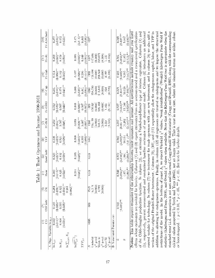
Table1:

TradeOpennessandIncome,1990-2011

(1)

(2)

(3)

(4)

(5)

(6)

(7)

(8)

(9)

(10)

(11)

(12)

CD

CDCnstr

FR

Base

BaseCnstr

TFP

IV-IMR

IV-IMR1

IV-Cap

IV-Lab

IV-All

IV-All-Cnstr

A.Dep.Variable

lnyj,t

lnLj,t

0.332

0.495

0.264

0.283

0.323

0.236

0.212

0.212

0.231

0.314

0.269

0.377

(0.041)∗∗

(0.035)∗∗

(0.038)∗∗

(0.044)∗∗

(0.037)∗∗

(0.033)∗∗

(0.045)∗∗

(0.045)∗∗

(0.044)∗∗

(0.066)∗∗

(0.060)∗∗

(0.025)∗∗

lnKj,t

0.460

0.505

0.322

0.425

0.432

0.524

0.507

0.507

0.474

0.442

0.459

0.452

(0.035)∗∗

(0.035)∗∗

(0.050)∗∗

(0.032)∗∗

(0.039)∗∗

(0.038)∗∗

(0.046)∗∗

(0.046)∗∗

(0.045)∗∗

(0.052)∗∗

(0.050)∗∗

(0.023)∗∗

ln∑ j6=iXij

0.264

(0.062)∗∗

ln(Πσ−1

j,t

)-0.214

-0.245

-0.099

-0.089

-0.089

-0.099

-0.107

-0.085

-0.171

(0.026)∗∗

(0.020)∗∗

(0.034)∗∗

(0.029)∗∗

(0.029)∗∗

(0.029)∗∗

(0.029)∗∗

(0.030)∗∗

(0.018)∗∗

TFPj,t

0.303

0.307

0.307

0.301

0.296

0.340

0.303

(0.088)∗∗

(0.097)∗∗

(0.097)∗∗

(0.099)∗∗

(0.101)∗∗

(0.081)∗∗

(0.026)∗∗

N1606

1606

1579

1579

1579

1447

1380

1380

1380

1380

1322

1322

UnderId

16.519

156.439

156.921

158.530

153.488

147.666

χ2p-val

(0.000)

(0.000)

(0.000)

(0.000)

(0.000)

(0.000)

WeakId

14.782

510.75

345.439

213.842

229.508

153.673

χ2p-val

(0.000)

(0.000)

(0.000)

(0.000)

(0.000)

(0.000)

Over

Id0.351

1.465

1.234

4.782

7.737

χ2p-val

(0.554)

(0.481)

(0.745)

(0.189)

(0.102)

B.StructuralParameters

α0.505

0.540

0.572

0.582

0.557

0.557

0.525

0.495

0.501

0.545

(0.035)**

(0.050)**

(0.046)**

(0.052)**

(0.054)**

(0.054)**

(0.054)**

(0.060)**

(0.053)**

(0.027)**

σ4.674

4.084

10.114

11.282

11.180

10.128

9.385

11.812

5.847

(0.580)**

(0.394)**

(2.817)**

(3.701)**

(3.632)**

(2.929)**

(2.547)**

(4.173)**

(0.620)**

Notes:Thistablereportsestimatesoftherelationship

betweentradeopennessandincome.

Allspecicationsincludecountryandyearxed

eects

whose

estimatesare

omittedforbrevity.

Columns(1)and(2)report

estimatesfrom

anunconstrained

andaconstrained

specication

oftheCobb-Douglasproductionfunction.In

column(3),

weestimate

aFrankel-and-Romer

typeofincomeregression.Columns(4)and

(5),

respectively,presentunconstrained

andconstrained

baselineestimatesofourstructuralmodel.Column(6)introducesanadditional

controlvariablefortechnology.

Incolumn(7)weinstrumentfortradeopennesswithournew

instrument,andin

column(8)wealsoadda

versionoftheoriginalFrankel-Romer

instrument.

Columns(9),(10),and(11)sequentiallyallow

forendogeneouscapital,labor,andTFPin

additionto

allow

ingforendogenousopenness.

Finally,in

column(12)allregressors

aretreatedasendogenousandweim

pose

thestructural

restrictionsofthemodel.In

thebottom

ofpanel

A,wereport

UnderIdχ2values,weakidentication(W

eakId)Kleibergen-PaapWald

Fstatistics(K

leibergen

andPaap,2006),andOverIdχ2values

when

available.Note

thattheKleibergen-PaapWald

testisappropriate

when

the

standard

errori.i.d.assumptionisnotmet

andtheusualCragg-Donald

Wald

statistic(C

raggandDonald,1993),alongwiththecorresponding

criticalvalues

proposedbyStock

andYogo(2005),are

nolonger

valid.Thisistruein

ourcase,wherethestandard

errors

are

either

robust

orbootstrapped.+p<

0.10,*p<.0

5,**p<.0

1.See

textforfurther

details.

47

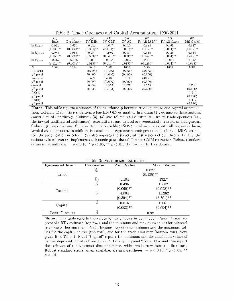
Table 2: Trade Openness and Capital Accumulation, 1990-2011(1) (2) (3) (4) (5) (6) (7) (8)Base BaseCnstr IV-IMR IV-GDP IV-All IV-All-LSDV IV-All-Cnstr Di-GMM

lnEj,t−1 0.011 0.016 0.012 0.007 0.010 0.083 0.061 0.047(0.003)∗∗ (0.003)∗∗ (0.004)∗∗ (0.004)+ (0.004)∗∗ (0.012)∗∗ (0.004)∗∗ (0.012)∗∗

lnKj,t−1 0.984 0.984 0.983 0.986 0.983 0.948 0.939 0.934(0.003)∗∗ (0.003)∗∗ (0.003)∗∗ (0.003)∗∗ (0.003)∗∗ (0.008)∗∗ (0.004)∗∗ (0.009)∗∗

lnPj,t−1 -0.052 -0.016 -0.047 -0.064 -0.065 -0.043 -0.061 -0.164(0.012)∗∗ (0.003)∗∗ (0.013)∗∗ (0.013)∗∗ (0.013)∗∗ (0.026)+ (0.004)∗∗ (0.083)∗

N 1684 1684 1602 1602 1602 1602 1602 1684UnderId 197.088 197.406 197.512 255.859χ2 p-val (0.000) (0.000) (0.000) (0.000)Weak Id 6899 4007 3190 243.210χ2 p-val (0.000) (0.000) (0.000) (0.000)OverId 0.388 4.559 2.921 1.553 3919χ2 p-val (0.533) (0.103) (0.232) (0.460) (0.000)AR(1) -1.210χ2 p-val (0.226)AR(2) -0.412χ2 p-val (0.680)

Notes: This table reports estimates of the relationship between trade openness and capital accumula-tion. Column (1) reports results from a baseline OLS estimator. In column (2), we impose the structuralconstraints of our theory. Columns (3), (4) and (5) report IV estimates, where trade openness (i.e.,the inward multilateral resistances), expenditure, and capital are sequentially treated as endogenous.Column (6) reports Least Squares Dummy Variable (LSDV) panel estimates with all regressors beingtreated as endogenous. In addition to treating all regressors as endogenous and using an LSDV estima-tor, the specication in column (7) also imposes the structural restrictions of our theory. Finally, theestimates in column (8) implements a dynamic panel-data dierence GMM estimator. Robust standarderrors in parentheses. + p < 0.10, * p < .05, ** p < .01. See text for further details.

Table 3: Parameter EstimatesRecovered From Parameter Min. Value Max. Value

η1 0.827Trade (0.135)**

tij 1.184 132.7α 0.495 0.582

(0.060)** (0.052)**Income

σ 4.084 11.282(0.394)** (3.701)**

δ 0.016 0.061Capital

(0.003)** (0.004)**

Cons. Discount β 0.98

Notes: This table reports the values for parameters in our model. Panel Trade re-ports the RTA estimate (top row), and the minimum and maximum values for bilateraltrade costs (bottom row). Panel Income reports the minimum and the maximum val-ues for the capital shares (top row), and for the trade elasticity (bottom row), frompanel B of Table 1. Panel Capital reports the minimum and the maximum values ofcapital depreciation rates from Table 2. Finally, in panel Cons. Discount we reportthe estimate of the consumer discount factor, which we borrow from the literature.Robust standard errors, when available, are in parentheses. + p < 0.10, * p < .05, **p < .01.

48

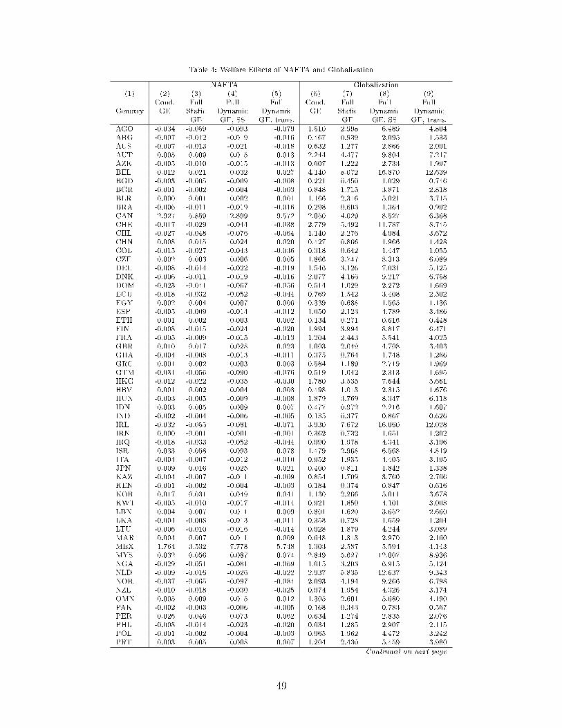
Table 4: Welfare Eects of NAFTA and Globalization

NAFTA Globalization(1) (2) (3) (4) (5) (6) (7) (8) (9)

Cond. Full Full Full Cond. Full Full FullCountry GE Static Dynamic Dynamic GE Static Dynamic Dynamic

GE GE, SS GE, trans. GE GE, SS GE, trans.AGO -0.034 -0.059 -0.093 -0.079 1.510 2.998 6.489 4.804ARG -0.007 -0.012 -0.019 -0.016 0.467 0.939 2.095 1.533AUS -0.007 -0.013 -0.021 -0.018 0.632 1.277 2.866 2.091AUT -0.005 -0.009 -0.015 -0.013 2.244 4.477 9.804 7.217AZE -0.005 -0.010 -0.015 -0.013 0.607 1.222 2.733 1.997BEL -0.012 -0.021 -0.032 -0.027 4.140 8.072 16.870 12.639BGD -0.003 -0.005 -0.009 -0.008 0.221 0.450 1.029 0.746BGR -0.001 -0.002 -0.004 -0.003 0.848 1.715 3.871 2.818BLR 0.000 -0.001 -0.002 -0.001 1.166 2.316 5.021 3.715BRA -0.006 -0.011 -0.019 -0.016 0.298 0.603 1.364 0.992CAN 2.927 5.859 12.899 9.572 2.050 4.029 8.527 6.368CHE -0.017 -0.029 -0.044 -0.038 2.779 5.492 11.787 8.745CHL -0.027 -0.048 -0.076 -0.064 1.140 2.276 4.984 3.672CHN -0.008 -0.015 -0.024 -0.020 0.427 0.866 1.966 1.428COL -0.015 -0.027 -0.043 -0.036 0.318 0.642 1.447 1.055CZE -0.002 -0.003 -0.006 -0.005 1.866 3.747 8.313 6.089DEU -0.008 -0.014 -0.022 -0.019 1.546 3.126 7.031 5.125DNK -0.006 -0.011 -0.019 -0.016 2.077 4.166 9.217 6.758DOM -0.023 -0.041 -0.067 -0.056 0.514 1.029 2.272 1.669ECU -0.018 -0.032 -0.052 -0.044 0.769 1.542 3.408 2.502EGY -0.002 -0.004 -0.007 -0.006 0.339 0.688 1.565 1.136ESP -0.005 -0.009 -0.014 -0.012 1.050 2.123 4.789 3.486ETH -0.001 -0.002 -0.003 -0.002 0.134 0.271 0.616 0.448FIN -0.008 -0.015 -0.024 -0.020 1.994 3.994 8.817 6.471FRA -0.005 -0.009 -0.015 -0.013 1.204 2.443 5.541 4.025GBR -0.010 -0.017 -0.028 -0.023 1.003 2.049 4.708 3.403GHA -0.004 -0.008 -0.013 -0.011 0.375 0.764 1.748 1.266GRC -0.001 -0.002 -0.003 -0.003 0.584 1.189 2.719 1.969GTM -0.031 -0.056 -0.090 -0.076 0.519 1.042 2.313 1.695HKG -0.012 -0.022 -0.035 -0.030 1.780 3.535 7.644 5.661HRV -0.001 -0.002 -0.004 -0.003 0.498 1.013 2.315 1.676HUN -0.003 -0.005 -0.009 -0.008 1.879 3.769 8.347 6.118IDN -0.003 -0.005 -0.009 -0.007 0.477 0.972 2.216 1.607IND -0.002 -0.004 -0.006 -0.005 0.185 0.377 0.867 0.626IRL -0.032 -0.055 -0.081 -0.071 3.930 7.672 16.060 12.028IRN 0.000 -0.001 -0.001 -0.001 0.362 0.732 1.651 1.202IRQ -0.018 -0.033 -0.052 -0.044 0.990 1.978 4.341 3.196ISR -0.033 -0.058 -0.093 -0.078 1.479 2.968 6.568 4.819ITA -0.004 -0.007 -0.012 -0.010 0.952 1.935 4.405 3.195JPN -0.009 -0.016 -0.025 -0.021 0.400 0.811 1.842 1.338KAZ -0.004 -0.007 -0.011 -0.009 0.854 1.709 3.760 2.766KEN -0.001 -0.002 -0.004 -0.003 0.184 0.374 0.847 0.616KOR -0.017 -0.031 -0.049 -0.041 1.130 2.266 5.011 3.678KWT -0.005 -0.010 -0.017 -0.014 0.921 1.850 4.101 3.008LBN -0.004 -0.007 -0.011 -0.009 0.801 1.620 3.652 2.660LKA -0.004 -0.008 -0.013 -0.011 0.358 0.728 1.659 1.204LTU -0.006 -0.010 -0.016 -0.014 0.928 1.879 4.244 3.089MAR -0.004 -0.007 -0.011 -0.009 0.648 1.313 2.970 2.160MEX 1.764 3.532 7.778 5.748 1.303 2.587 5.594 4.143MYS -0.032 -0.056 -0.087 -0.074 2.849 5.627 12.007 8.936NGA -0.029 -0.051 -0.081 -0.069 1.615 3.203 6.915 5.124NLD -0.009 -0.016 -0.026 -0.022 2.937 5.835 12.637 9.343NOR -0.037 -0.065 -0.097 -0.084 2.093 4.194 9.266 6.798NZL -0.010 -0.018 -0.030 -0.025 0.974 1.954 4.326 3.174OMN -0.005 -0.009 -0.015 -0.012 1.305 2.601 5.680 4.190PAK -0.002 -0.003 -0.006 -0.005 0.168 0.343 0.783 0.567PER -0.026 -0.046 -0.073 -0.062 0.634 1.274 2.835 2.076PHL -0.008 -0.014 -0.023 -0.020 0.634 1.285 2.907 2.115POL -0.001 -0.002 -0.004 -0.003 0.965 1.962 4.472 3.242PRT -0.003 -0.005 -0.008 -0.007 1.204 2.430 5.459 3.980

Continued on next page

49

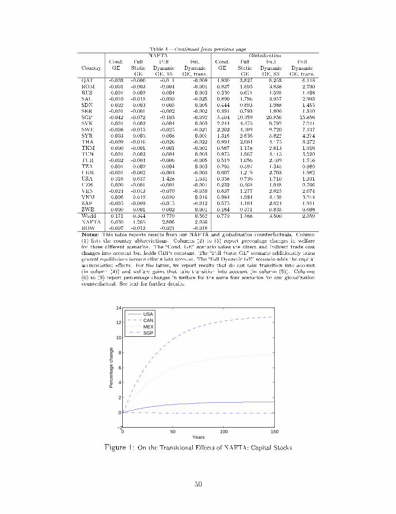
Table 4 Continued from previous page

NAFTA GlobalizationCond. Full Full Full Cond. Full Full Full

Country GE Static Dynamic Dynamic GE Static Dynamic DynamicGE GE, SS GE, trans. GE GE, SS GE, trans.

QAT -0.003 -0.006 -0.011 -0.009 1.930 3.827 8.253 6.118ROM -0.001 -0.003 -0.004 -0.004 0.837 1.695 3.838 2.790RUS -0.001 -0.002 -0.004 -0.003 0.330 0.671 1.528 1.108SAU -0.010 -0.018 -0.030 -0.025 0.890 1.786 3.957 2.903SDN -0.002 -0.003 -0.005 -0.005 0.444 0.893 1.988 1.455SER -0.001 -0.001 -0.002 -0.002 0.391 0.793 1.806 1.310SGP -0.042 -0.072 -0.105 -0.092 5.404 10.359 20.856 15.856SVK -0.001 -0.002 -0.004 -0.003 2.244 4.475 9.792 7.211SWE -0.008 -0.015 -0.025 -0.021 2.202 4.409 9.720 7.137SYR -0.003 -0.005 -0.008 -0.007 1.316 2.636 5.822 4.274THA -0.009 -0.016 -0.026 -0.022 0.994 2.004 4.475 3.272TKM 0.000 -0.001 -0.001 -0.001 0.587 1.178 2.613 1.916TUN -0.001 -0.002 -0.004 -0.003 0.975 1.967 4.415 3.220TUR -0.002 -0.004 -0.006 -0.005 0.519 1.056 2.409 1.746TZA -0.001 -0.002 -0.004 -0.003 0.295 0.597 1.345 0.980UKR -0.001 -0.002 -0.003 -0.003 0.607 1.219 2.703 1.982USA 0.316 0.637 1.428 1.031 0.358 0.736 1.710 1.231UZB 0.000 -0.001 -0.001 -0.001 0.232 0.468 1.048 0.766VEN -0.024 -0.043 -0.070 -0.059 0.637 1.277 2.825 2.074VNM -0.006 -0.012 -0.020 -0.016 0.984 1.984 4.438 3.244ZAF -0.005 -0.009 -0.015 -0.012 0.575 1.164 2.624 1.911ZWE 0.000 -0.001 -0.002 -0.001 0.184 0.371 0.835 0.608World 0.171 0.344 0.770 0.562 0.779 1.568 3.500 2.559NAFTA 0.630 1.265 2.806 2.056ROW -0.007 -0.013 -0.021 -0.018Notes: This table reports results from our NAFTA and globalization counterfactuals. Column(1) lists the country abbreviations. Columns (2) to (5) report percentage changes in welfarefor three dierent scenarios. The Cond. GE scenario takes the direct and indirect trade costchanges into account but holds GDPs constant. The Full Static GE scenario additionally takesgeneral equilibrium income eects into account. The Full Dynamic GE scenario adds the capitalaccumulation eects. For the latter, we report results that do not take transition into account(in column (4)) and welfare gains that take transition into account (in column (5)). Columns(6) to (9) report percentage changes in welfare for the same four scenarios for our globalizationcounterfactual. See text for further details.

0 50 100 150−2

0

2

4

6

8

10

12

14

Years

Per

cent

age

chan

ge

USACANMEXSGP

Figure 1: On the Transitional Eects of NAFTA: Capital Stocks

50