greenhouse gas Emissions from - BIOEN FAPESPbioenfapesp.org/scopebioenergy/images/chapters/bioen-scope_chapte… · greenhouse gas Emissions from ... The GHG Protocol Product Standard,

greenhouse gas Emissions from

Bioenergy

Isaias de Carvalho Macedo*a†, André M. Nassar*b‡, Annette L. Cowiec, Joaquim E.A. Seabraa, Luisa Marellid, Martina Ottoe, Michael Q. Wangf, and Wallace E. Tynerg

*Lead Authors Responsible SAC: Jeremy Woods

Associate Editor: Paulo Eduardo Artaxo Netto Contact: †[email protected]; ‡[email protected]

aUniversidade Estadual de Campinas, Brazil; bAgroicone, Brazil;

cUniversity of New England, Australia; dEuropean Commission, Italy;

eUnited Nations Environmental Programme, France; fArgonne National Laboratory, USA;

gPurdue University, USA

chapter 17

583Bioenergy & Sustainability

highlights ● Biofuels in suitable conditions can provide substantial levels of GHG mitigation.

Co- and by-product utilization can improve this effect

● Second generation biofuels may show higher GHG mitigation, to be demonstrated in full scale commercial operation

● LUC studies for better biofuels evidence the great improvement potential for the whole agriculture / forestry system

● Further development of GHG LCA methodologies is needed to quantify the influence of timing of emissions and removals, albedo change, and short-lived climate forcing agents. New data will be required in order to apply these methods

● Tools to help provide technical support for public policies have been developed and are being implemented.

SummaryRecent advances in modeling and access to new data have enabled advances in greenhouse gas (GHG) emissions estimation. Current methodological issues (e.g., treatment of indirect land use change (iLUC) and co-products) are presented, as well as current knowledge on climate change impacts other than GHGs (timing of GHG emissions / removals; albedo changes; aerosols emissions). Commercial biofuels in suitable conditions can provide moderate levels of GHG mitigation, and second generation biofuels may show higher GHG mitigation. Ethanol from sugarcane shows the largest “average” net GHG mitigation today; biodiesel (many sources; Europe) provides 30 – 60% mitigation (no LUC considered) compared with diesel; commercial biopower from solid biomass produces emissions typically ranging from 26 to 48 gCO2e / kWh (systems > 10 MWe), providing substantial net GHG mitigation. There is still considerable uncertainty surrounding the quantification of emissions associated to iLUC but recent studies tend to converge toward the lower level of the range of estimates. At the time of the prior SCOPE report (SCOPE 2009), the magnitude of LUC emissions was felt to be large enough to negate the GHG emission benefits of an otherwise low-emitting biomass-based fuel supply chain. Five years later, this is no longer the case for ethanol crops as illustrated in this document. LUC emissions can be avoided if land demand for biofuels expansion is managed, if yield increase exceeds increase in demand and as

584

chapter 17 Greenhouse Gas Emissions from Bioenergy

Bioenergy & Sustainability

long as deforestation rates are decreasing. Implementation of methods to provide the data needed to support policies and strategic decisions is discussed. Recommendations include continued support i) for technology development, and data acquisition for GHG evaluation; ii) to clarify some GHG emissions issues; iii) to implement methodologies and policies to maximize biofuels GHG emissions benefits such as zoning systems, policies for deforestation control and monitoring; good practices in agriculture; intensification of land use (discussed in Chapter 9, this volume).

17.1 IntroductionThe implementation of efficient bioenergy has been considered essential to reduce and stabilize GHG emission levels in the next decades. The last five years have seen important efforts to improve models and obtain more reliable data on key parameters (e.g., soil carbon stocks and N2O emission coefficients) (JRC 2010a; Winrock 2009a; Winrock 2009b, FAO/IIASA/ISRIC/ISS-CAS/JRC 2008), both globally and for specific regions (Galdos et al. 2009; Mello et al, 2014), as well as the estimation of unobservable phenomena such as indirect land use changes (JRC 2010b; JRC 2011; Dunn et al. 2013), and to support and help improve the contribution of bioenergy to GHG mitigation, and guide policy decisions.

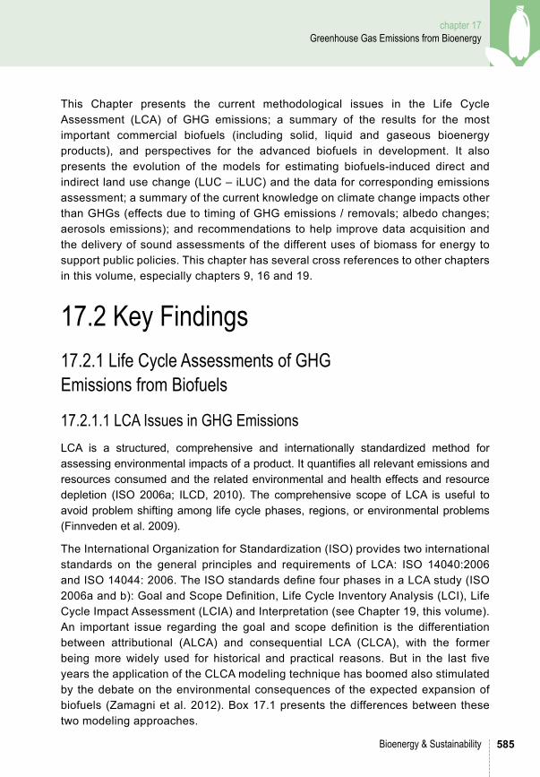
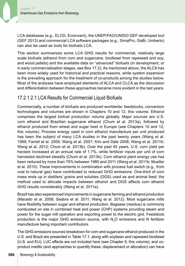
Figure 17.1. Mass flows and life cycle GEE emissions in production of ethanol from sugarcane.

585



This Chapter presents the current methodological issues in the Life Cycle Assessment (LCA) of GHG emissions; a summary of the results for the most important commercial biofuels (including solid, liquid and gaseous bioenergy products), and perspectives for the advanced biofuels in development. It also presents the evolution of the models for estimating biofuels-induced direct and indirect land use change (LUC – iLUC) and the data for corresponding emissions assessment; a summary of the current knowledge on climate change impacts other than GHGs (effects due to timing of GHG emissions / removals; albedo changes; aerosols emissions); and recommendations to help improve data acquisition and the delivery of sound assessments of the different uses of biomass for energy to support public policies. This chapter has several cross references to other chapters in this volume, especially chapters 9, 16 and 19.

17.2 Key Findings17.2.1 life Cycle Assessments of ghg Emissions from Biofuels

17.2.1.1 lCA Issues in ghg EmissionsLCA is a structured, comprehensive and internationally standardized method for assessing environmental impacts of a product. It quantifies all relevant emissions and resources consumed and the related environmental and health effects and resource depletion (ISO 2006a; ILCD, 2010). The comprehensive scope of LCA is useful to avoid problem shifting among life cycle phases, regions, or environmental problems (Finnveden et al. 2009).

The International Organization for Standardization (ISO) provides two international standards on the general principles and requirements of LCA: ISO 14040:2006 and ISO 14044: 2006. The ISO standards define four phases in a LCA study (ISO 2006a and b): Goal and Scope Definition, Life Cycle Inventory Analysis (LCI), Life Cycle Impact Assessment (LCIA) and Interpretation (see Chapter 19, this volume). An important issue regarding the goal and scope definition is the differentiation between attributional (ALCA) and consequential LCA (CLCA), with the former being more widely used for historical and practical reasons. But in the last five years the application of the CLCA modeling technique has boomed also stimulated by the debate on the environmental consequences of the expected expansion of biofuels (Zamagni et al. 2012). Box 17.1 presents the differences between these two modeling approaches.

586



ALCA and CLCA, from their logic, represent the two fundamentally different situations of modeling the analyzed system (ILCD, 2010). ALCA focuses on the environmentally relevant physical flows to and from a life cycle and its subsystems, to describe the impacts of the average unit of a product, while CLCA describes how environmentally relevant flows will change in response to decisions (Finnveden et al. 2009). In attributional modeling the system is modeled as it is or was (or is forecast to be), whereas CLCA models a hypothetic generic supply-chain prognosticated along market-mechanisms, and potentially including political interactions and consumer behavior changes (ILCD 2010). CLCA first appeared as a discussion in Weidema (1993), which broadly outlined the need to consider market information in life cycle inventory data.

The different focuses of attributional and consequential LCA are reflected in several methodological choices in LCA, for instance, when discussing system boundaries, data collection and allocation (Finnveden et al. 2009). The approach for solving multifunctional processes is one of the most critical issues in LCA. According to the ISO (2006b) hierarchy, wherever possible, allocation should be avoided by process subdivision, or by expanding the product system to include the additional functions related to the co-products for solving multifunctionality (ILCD 2010).

Where allocation cannot be avoided, the ISO standards (ISO 2006b) advise that the “inputs and outputs of the system should be partitioned between its different products or functions in a way that reflects underlying physical relationships between them”. Lastly, (ISO 2006c) “where physical relationship alone cannot be established or used as the basis for allocation, the inputs should be allocated between the products and functions in a way that reflects other relationships between them” (e.g., economic value of the products).

LCA considers aspects of environment, human health and resource use, but the challenges posed by climate change have brought special attention to the emissions of GHGs in the life cycle of products. New standards and methods over the last years focused on the assessment of the life cycle GHG emissions and removals (also referred to as carbon footprint) of products. The GHG Protocol Product Standard, PAS 2050:2011 and ISO/TS 14067:2013 are examples of these new standards, while the Roundtable on Sustainable Biomaterials GHG Calculation Methodology (RSB 2011)

Box 17.1. Attributional lCA (AlCA) versus Consequential lCA (ClCA)

587



is an example of a specific method developed in the context of biofuels certification. In general, these standards are founded on the same basic principles set in the ISO LCA standards, with the difference that they address only one impact category (climate change), and provide more specific guidance for some methodological aspects (e.g., how to deal with land use change). Figure 17.1 exemplifies the topics in the evaluation of life cycle GHG emissions for a commercial biofuel.

In the context of biofuels policies, regional regulatory schemes have used different approaches based on the LCA technique to estimate GHG emissions. For example, the impact assessment developed by the U.S. Environmental Protection Agency (EPA) for the Renewable Fuel Standard – RFS2 (EPA 2010) and the analysis performed by the California Air Resources Board (CARB) for the Low Carbon Fuel Standard (CARB 2009) vary greatly between themselves, and also in comparison with the European Commission’s Renewable Energy Directive (EU-RED), (EC 2009). Agricultural aspects, allocation procedures and economic modeling approaches for iLUC assessments are the major areas where methodological divergences exist (Khatiwada et al. 2012). In terms of the modeling approach, EU-RED is largely consistent with ALCA methodology, with the exception of the treatment of excess electricity from cogeneration. However, inconsistencies may be created in the future if the European Commission develops a method for indirect effects, a consequential issue (Brander et al. 2009). The EPA assessment is fully based on consequential modeling, while the CARB analysis includes some elements of ALCA.

17.2.1.2 lCA Results of greenhouse gas Emissions for BiofuelsMany LCA studies address energy use and greenhouse gas (GHG) emissions of biofuels vs. conventional petroleum fuels. In 1990s and early 2000s, studies addressed energy balance (or energy ratio) of biofuels. Biofuels usually have a positive energy balance (energy ratio greater than one) (e.g., see Wang et al. 2012 for ethanol energy results).

Biofuel GHG LCA results vary considerably among different biofuel types and regions; the GHG benefit of biofuel use depends on the actual fossil fuel displacement and on the life cycle GHG emissions of the displaced fossil fuel. Biofuel LCA GHG results also are affected by LCA methodology, including technology modeling and data availability. The issues include LCA approach, LCA system boundary, treatment of biofuel co-products, modeling of LUC, and how to include technology advancement over time (Menichetti 2008; Gnansounou et al. 2009; Cherubini et al. 2009).

Regional biofuel regulations such as the EU Renewable Fuel Directive (RED), the U.K. Renewable Transport Fuel Obligation (RTFO), the California Low Carbon Fuel Standard (LCFS), and the U.S. EPA Renewable Fuel Standard (RFS) require estimation of life cycle GHG emissions of biofuels. Several LCA models are available for this estimation, including the Argonne National Laboratory GREET model (GREET 2012) and the U. C. Davis Model (Delucchi 2003) in the U.S., the GHGenius model in Canada, and the E3 Database and Biograce (LBSM 2013; BioGrace 2013) in Europe.

588



LCA databases (e.g., ELCD, Ecoinvent), the UNEP/FAO/UNIDO GEF developed tool (GEF 2013) and commercial LCA software packages (e.g., SimaPro, GaBi, Umberto) can also be used as tools for biofuels LCA.

This section summarizes some LCA GHG results for commercial, relatively large scale biofuels (ethanol from corn and sugarcane, biodiesel from rapeseed and soy, and wood pellets) and the available data on “advanced” biofuels (in development, or in early commercialization stages, see Box 17.2). As mentioned above, the ALCA has been more widely used for historical and practical reasons, while system expansion is the prevailing approach for the treatment of co-products among the studies below. Most of the analyses have employed elements of ALCA and CLCA as the discussion and differentiation between these approaches became more evident in the last years.

17.2.1.2.1 lCA Results for Commercial liquid BiofuelsCommercially, a number of biofuels are produced worldwide; feedstocks, conversion technologies and volumes are shown in Chapters 10 and 12, this volume. Ethanol comprises the largest biofuel production volume globally. Major sources are U.S. corn ethanol and Brazilian sugarcane ethanol (Chum et al. 2013a), followed by ethanol produced from wheat and sugar beet in Europe (see Chapters 10 and 12, this volume). Process energy used in corn ethanol manufacture per unit produced has been the subject of many LCA studies in the past twenty years (Wang et al. 1999; Farrell et al. 2006; Wang et al. 2007; Kim and Dale 2008; Wang et al. 2011b; Wang et al. 2012; Chum et al. 2013b). Over the past 40 years, U.S. corn yield per hectare increased at an annual rate of 1.7%, while fertilizer inputs per unit of corn harvested declined steadily (Chum et al. 2013b). Corn ethanol plant energy use has been reduced by more than 70% between 1980 and 2011 (Wang et al. 2011b; Mueller et al. 2010). These improvements in combination with process fuel switch (e.g., from coal to natural gas) have contributed to reduced GHG emissions. One-third of corn mass ends up in distillers’ grains and solubles (DGS) used as and animal feed; the method used to allocate impacts between ethanol and DGS affects corn ethanol GHG results considerably (Wang et al. 2011a).

Brazil has also experienced improvements in sugarcane farming and ethanol production (Macedo et al. 2008; Seabra et al. 2011; Wang et al. 2012). Most sugarcane mills have flexibility between sugar and ethanol production. Bagasse (residue) is commonly combusted on site in combined heat and power (CHP) systems providing steam and power for the sugar mill operation and exporting power to the electric grid. Feedstock production is the major GHG emission source, with N2O emissions and N fertilizer manufacture being important contributors.

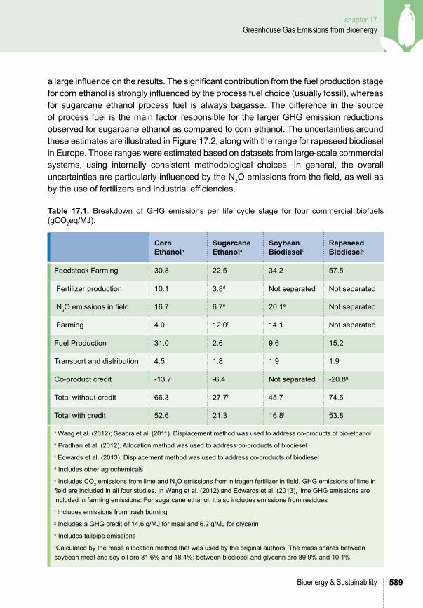
The GHG emissions sources breakdown for corn and sugarcane ethanol produced in the U.S. and Brazil are presented in Table 17.1, along with soybean and rapeseed biodiesel (U.S. and EU); LUC effects are not included here (see Chapter 9, this volume); and co-product credits (and approaches to quantify these: displacement or allocation) can have

589



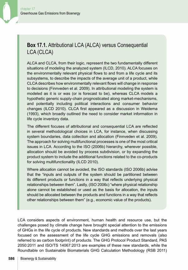
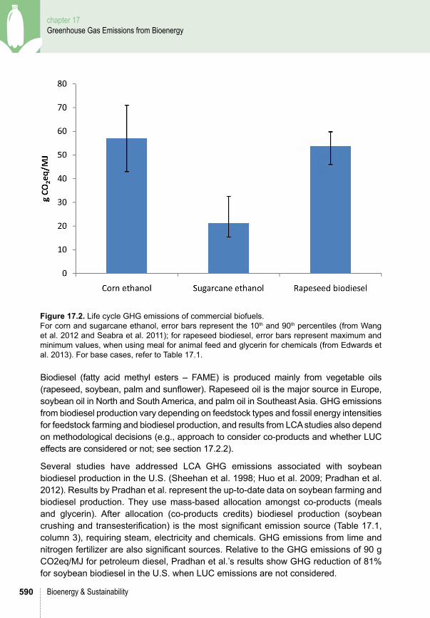
a large influence on the results. The significant contribution from the fuel production stage for corn ethanol is strongly influenced by the process fuel choice (usually fossil), whereas for sugarcane ethanol process fuel is always bagasse. The difference in the source of process fuel is the main factor responsible for the larger GHG emission reductions observed for sugarcane ethanol as compared to corn ethanol. The uncertainties around these estimates are illustrated in Figure 17.2, along with the range for rapeseed biodiesel in Europe. Those ranges were estimated based on datasets from large-scale commercial systems, using internally consistent methodological choices. in general, the overall uncertainties are particularly influenced by the N2O emissions from the field, as well as by the use of fertilizers and industrial efficiencies.

Table 17.1. Breakdown of GHG emissions per life cycle stage for four commercial biofuels (gCO2eq/MJ).

Corn Ethanola

Sugarcane Ethanola

Soybean Biodieselb

Rapeseed Biodieselc

Feedstock Farming 30.8 22.5 34.2 57.5

Fertilizer production 10.1 3.8d Not separated Not separated

N2O emissions in field 16.7 6.7e 20.1e Not separated

Farming 4.0 12.0f 14.1 Not separated

Fuel Production 31.0 2.6 9.6 15.2

Transport and distribution 4.5 1.8 1.9 1.9

Co-product credit -13.7 -6.4 Not separated -20.8g

total without credit 66.3 27.7h 45.7 74.6

total with credit 52.6 21.3 16.8i 53.8

a Wang et al. (2012); Seabra et al. (2011). Displacement method was used to address co-products of bio-ethanolb Pradhan et al. (2012). Allocation method was used to address co-products of biodieselc Edwards et al. (2013). Displacement method was used to address co-products of biodieseld includes other agrochemicalse Includes CO2 emissions from lime and N2O emissions from nitrogen fertilizer in field. GHG emissions of lime in field are included in all four studies. In Wang et al. (2012) and Edwards et al. (2013), lime GHG emissions are included in farming emissions. For sugarcane ethanol, it also includes emissions from residuesf Includes emissions from trash burningg Includes a GHG credit of 14.6 g/MJ for meal and 6.2 g/MJ for glycerinh includes tailpipe emissionsi Calculated by the mass allocation method that was used by the original authors. The mass shares between soybean meal and soy oil are 81.6% and 18.4%; between biodiesel and glycerin are 89.9% and 10.1%

590



Biodiesel (fatty acid methyl esters – FAME) is produced mainly from vegetable oils (rapeseed, soybean, palm and sunflower). Rapeseed oil is the major source in Europe, soybean oil in North and South America, and palm oil in Southeast Asia. GHG emissions from biodiesel production vary depending on feedstock types and fossil energy intensities for feedstock farming and biodiesel production, and results from LCA studies also depend on methodological decisions (e.g., approach to consider co-products and whether LUC effects are considered or not; see section 17.2.2).

Several studies have addressed LCA GHG emissions associated with soybean biodiesel production in the U.S. (Sheehan et al. 1998; Huo et al. 2009; Pradhan et al. 2012). Results by Pradhan et al. represent the up-to-date data on soybean farming and biodiesel production. They use mass-based allocation amongst co-products (meals and glycerin). After allocation (co-products credits) biodiesel production (soybean crushing and transesterification) is the most significant emission source (Table 17.1, column 3), requiring steam, electricity and chemicals. GHG emissions from lime and nitrogen fertilizer are also significant sources. Relative to the GHG emissions of 90 g CO2eq/MJ for petroleum diesel, Pradhan et al.’s results show GHG reduction of 81% for soybean biodiesel in the U.S. when LUC emissions are not considered.

Figure 17.2. Life cycle GHG emissions of commercial biofuels. For corn and sugarcane ethanol, error bars represent the 10th and 90th percentiles (from Wang et al. 2012 and Seabra et al. 2011); for rapeseed biodiesel, error bars represent maximum and minimum values, when using meal for animal feed and glycerin for chemicals (from Edwards et al. 2013). For base cases, refer to Table 17.1.

591



Edwards et al. (2013) assessed biodiesel produced from rapeseed, sunflower and soybean, using the substitution method to consider meal and glycerin co-produced. Rapeseed farming is by far the largest GHG emission source, 68% higher than that of soybean farming in the U.S.. Excluding LUC emissions, Edwards et al. (2013) estimated average GHG emissions of biodiesel at 37-59, 46, 55-60, and 31-63 g CO2eq/MJ for rapeseed, sunflower, soybean and palm oil, respectively, leading to GHG emission reductions of 33-58%, 48%, 32-38%, 29-65% if displacing petroleum diesel (GHG emission rate of 88.6 g CO2eq/MJ). The range for each option reflects different uses for meals and glycerin; the low-end value for each option represents the case where glycerin is used in anaerobic digestion, which might be the only option if other glycerin markets become saturated as biodiesel production grows.

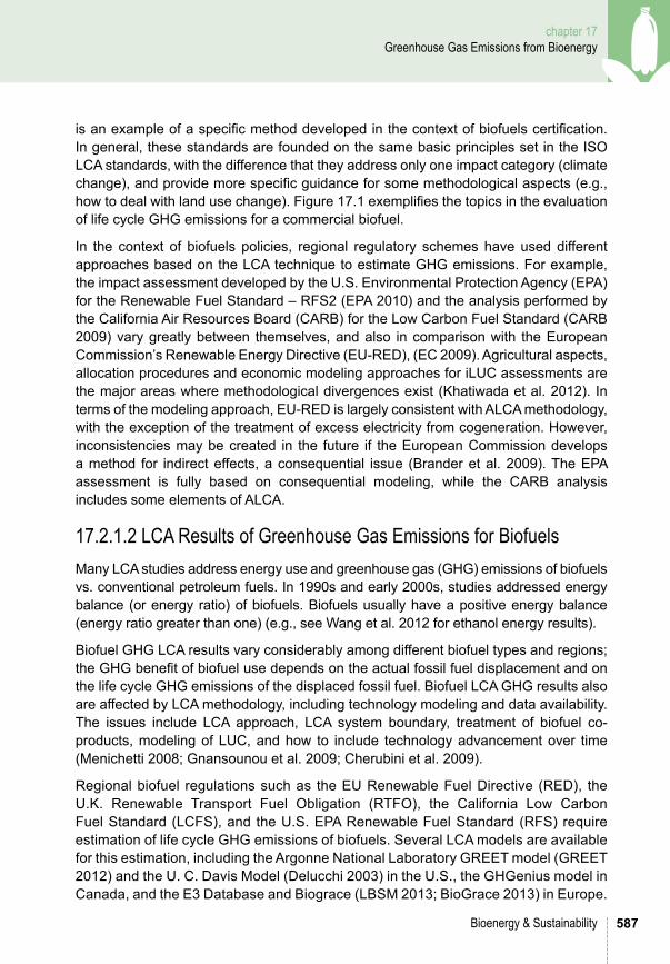
Advanced biofuels have not yet reached commercial, large scale production and LCA of GHG emissions are estimates based on projections from different stages of development, technical data, and methodology choices (Box 17.2). Recent results for cellulosic ethanol are shown in Wang et al. (2012); and reviews are presented, among others, in Borrion et al. (2012) and Wiloso et al. (2012). Results from a meta regression analysis based on published data for cellulosic ethanol and BtL (synthetic diesel) emissions are shown in Figure 17.3 (Menten et al. 2013).

Figure 17.3. Meta-regression analysis based on projected second generation (2G) biofuels literature data for cellulosic ethanol and BtL (diesel) routes (after Menten et al. 2013); see Box 17.2. First two columns for EU results; columns 3 and 4 for North America results. -Data Base: 516 observations (G2) in 47 selected studies, 2003 – 2012; 314 ethanol, 202 synthetic diesel; 51% including LUC (less than 10% including iLUC); 97% using CLCA, 3% ALCA; 53% from EU, 45% from North America. -Vertical bars: 95% confidence interval - Reference fossil fuel emissions: EU (83.8 g CO2eq/MJ for both gasoline and diesel); U.S. (92.5 g CO2eq / MJ, average of gasoline and diesel references, for both).

592



Box 17.2. Estimated lCA results for advanced biofuelsAdvanced biofuels here refer to biofuels in development or early commercialization stages; sometimes called “second generation” (G2) biofuels (cellulosic based, thermochemical or biochemical processing) and “third generation” (oils produced by algae). Research and development efforts are helping advance cellulosic biofuels technology and economics. Pilot and commercial scale plants recently began to come online in the U.S., Europe and Brazil. Cellulosic feedstocks with large potentials are crop residues, bagasse in sugar mills, perennial grasses, woody plants, and forest residues. Feedstock supply, including collection, transportation, and storage cause different levels of GHG emissions depending on feedstock type, location and system design. Processes for feedstock pre-treatment and conversion also lead to significant differences in GHG emissions. Cellulosic ethanol plants can use residues such as lignin to generate steam and electricity with CHP; and electricity export to electric grid can help improve plant economics and reduce GHG footprint. Results from Wang et al. (2012) suggest that cellulosic ethanol is projected to have larger GHG emission reductions compared to gasoline than the current commercial biofuels. Since there is no commercial scale production, almost all results come from estimates projected for different processes and feedstocks, at pilot plant (and even laboratory) scale. A meta regression analysis of the literature results on cellulosic ethanol and biomass to synthetic diesel (thermochemical, BtL) processes support these projected higher decreases in GHG emissions (Menten et al. 2013), Figure 17.3; however the systematic difference between North American and European estimates, and ethanol and BtL, remains to be fully explained.

17.2.1.2.2 lCA Results for Solid BiofuelsCommercial solid biomass utilization (e.g., power production and indoor heating using household or district heating systems) has grown significantly in the last decade; estimated consumption of wood pellets in EU alone was 12 million t/year, in 2012 (NREL 2013). In 2011, the EU started evaluating binding EU-wide Standards, including GHG emissions.Table 17.2 shows the results of a recent, comprehensive analysis using data from 387 references; GHG emissions vary according to scale, feedstock and technology.

593



Table 17.2. LCA GHG emissions (excluding LUC): commercial biopower generation technologiesa.

Feedstock Development stage

Lifecycle GHG Emissions, gCO2eq/kWh c

>10 MWe avg

>10 MWe range

0.01-10 MWe avg

0.01-10 MWe range

Electrical efficiencyb Electrical efficiencyb

31.5% 27-36% 20% 10-30%

Wood waste and forest residues

Commercial 26 23-30 40 27-80

Agriculture residues

Commercial and developing with respect to logistics collection and preprocessing

48 42-56 75 50-151

Short rotation woody crops

Commercial and developing with respect to crops and logistics

35 31-40 55 37-109

Herbaceous crops developing 56 49-64 40 59-173

a Courtesy of the Sustainability Information Exchange Database, Ethan Warner, NREL (2013). Data sources and meta-model: Warner et al (2013) including 387 references through June 2011 of which 117 LCAs passed quality and relevance screens in the harmonization process. Efficiency data for biopower systems from Bruckner et al. (2011) and IEA Bioenergy (2010)b Ranges represent electrical efficiency end point values c As references, the fossil fuel combustion GHG emissions in thermo-electric power plants, with their variation due to different technology levels, are: i) coal: 1000 g CO2eq / kWhe; (800 – 1300) g CO2eq / kWhe; ii) oil: 800 g CO2eq / kWhe; iii) natural gas: 550 g CO2eq / kWhe; (400 – 800) g CO2eq / kWhe (Weisser 2007)

For any form of bioenergy – current or advanced, solid or liquid – the avoidance of GHG emissions on a life cycle basis increases as the efficiency of feedstock production and conversion improves, and as the penetration of renewables increases in the overall energy matrix. With respect to the latter point, consider for example a biofuel pathway with process energy provided by unfermented residues, as it is the current case for sugarcane ethanol and is anticipated for most cellulosic biofuels. Such pathway has greater than zero life cycle GHG emissions today in good part because of the fossil energy used in the ancillary processes involved in the production cycle: fertilizer manufacture, feedstock cultivation, harvesting and transport, and product distribution. As the energy matrix progresses toward being low-carbon, the emissions associated with these ancillary processes is reduced proportionately and the life cycle GHG emissions will be lower. In Brazil, for instance, the increasing biodiesel blend in diesel (6% volume today) and the increasing substitution of bagasse generated energy for thermo electricity (in the margin) is expected to substantially reduce sugarcane ethanol life cycle GHG emissions.

594



17.2.2 land Use Changes and ghg EmissionsLUC has been the most contentious issue in evaluating GHG effects of biofuels. LUCs can lead to a reduction or an increase of C stocks in biomass and soil, thus affecting the net GHG emissions from the bioenergy system. The causes behind LUC are multiple, complex, interlinked, and change over time. This makes quantification of GHG emissions and C sequestration associated with LUC inherently uncertain and studies report widely different results. Bioenergy projects may also indirectly reduce LUC pressures, such as when the ethanol co-product DGS displaces soy as animal feed, reducing the direct LUC (dLUC) pressure associated with increasing soy demand.

Especially the inclusion of iLUC adds greatly to the uncertainty in quantifications of LUC effects. Because agricultural markets are integrated and supply response to shocks in demand can take place in various producing regions, LUC estimates have to be calculated globally. LUC estimates, therefore, can only be determined using global models, which are highly uncertain, because the available models are based on unobservable and unverifiable parameters and are dependent on assumed policy, economic contexts, and exogenous inputs. Models results, therefore, can only be verifiable if all conditions are also met in the reality.

For conceptual reasons, it is important to distinguish between dLUC and iLUC. Direct LUC accounts for changes in land used associated with the direct expansion of biofuel feedstock production, such as the displacement of food or fiber crops, pastures and commercial forests or the conversion of natural ecosystems. Indirect LUC comprises induced effects of biofuel feedstock expansion promoting land use changes elsewhere than where the expansion has taken place. For example, natural ecosystems can be displaced elsewhere in order to re-establish market equilibrium compensating for the losses in food/fiber production caused by the bioenergy project.

Bioenergy emissions associated to LUC are measured through three steps: dLUC and iLUC are accounted in area amount through global models; dLUC in area amount is translated into total emissions and total emissions are converted to an iLUC factor dividing it by bioenergy production. Emissions are estimated for the direct displacement caused by the biofuel crop and the direct displacement caused by another land use but as a result of the bioenergy crop expansion.

Although dLUC and iLUC are conceptually different, models capture both effects together. An iLUC factor, therefore, is a result of a combination between dLUC and iLUC. Differently than iLUC, dLUC patterns can theoretically be established through satellite images or secondary data and used as evidences for calibrating models. When measured in projections, however, both are determined by models scenarios. iLUC not being empirically observable, the estimation of an iLUC factor depends on assumptions of cause-effect relations that will attribute responsibility of land conversion to individual agricultural land uses.

595



Most of the attempts to quantify LUC and associated GHG emissions have used general or partial equilibrium models of varying scope concerning geography and spatial resolution, sectors covered and detail in their characterization (Keeney and Hertel 2009; Kretschmer and Peterson 2010; Lapola et al. 2010; Taheripour et al. 2011; Laborde 2011; Khanna and Crago 2012; Havlik et al. 2013). Alternative approaches include statistical analyses (Barona et al. 2010; Arima et al. 2011) and quantifications based on pre-defined causal-effect chains, where specific LUC patterns are assigned to specific biofuels/feedstocks grown on specified land types (Tipper and Brander 2009; Bauen et al. 2010; Fritsche et al. 2010; Kim and Dale 2009; Moreira et al. 2012). A stylized way of grouping modeling approaches for assessing LUC is to divide them in four families (Wicke et al. 2014), namely, computable general equilibrium models (CGE), partial equilibrium models (PE), bottom-up analysis and integrated assessment models (IAM).

Net GHG emissions associated with LUC are obtained by combining the LUC quantification outcome with data on GHG emissions associated with the specific types of LUC that are obtained. Equilibrium models with detailed biofuel features, incorporation of animal feeds, and revision of economic parameters (price elasticities of crop yields and demand) have been developed in the last years. Databases and models to quantify GHG emissions associated with LUC are continuously improved (Dunn et al. 2013; JRC 2010b; JRC 2011). Yet, limitations in methodology and data make quantification of iLUC emissions and identification of causal mechanisms behind iLUC highly contentious issues (Gao et al. 2011; Mathews and Tan 2009; Nassar et al. 2011; Prins et al. 2010). Equilibrium models, unless explicitly represented in scenarios, are not capable of capturing certain long-term changes, particularly considering innovation and paradigm shifts within agriculture systems. One strong example is the double crops systems that are still not represented in CGE models.

Nevertheless, considering the global nature of iLUC effects, global models, both general and partial, are up to now the most suitable methodology available for quantifying land use effects. The main weakness of the models, besides the methodological issues already mentioned, is that they are not friendly for policy makers and they give responses to specific conditions rather than generalized situations as expected by governments and legislators. Therefore, in general, policy makers are not confident in using their results for policy decisions.

17.2.2.1 models Results: ilUC FactorsEstimated LUC emissions are usually presented in two formats: iLUC factors, i.e., CO2e per unit of energy output, and area amount, i.e., hectares per unit of energy output. The majority of the studies present results in iLUC factors but due to the additional uncertainty that is added in the simulations related to the methodology used to translate area amount changes into emissions, some studies only present results in area amount (Taheripour and Tyner 2013; Elobeid et al. 2011).

596



Available model-based studies have found changes in land use as a result of biofuels feedstocks expansion, therefore resulting in positive iLUC factors. A comprehensive sample of iLUC factors results is presented in Table 17.3, which was inspired by and is an update of Figure 1 in Wicke et al. (2012). There are two main underlying reasons for models to estimate positive net LUC: they are not calibrated to allow productivity increase to compensate higher demand for biofuels and they assume that any expansion in production will require additional conversion of native vegetation land.

Table 17.3 shows results from a selection of studies of ethanol from corn, sugarcane and sugarbeet and biodiesel from palm, rape and soy. Results show that uncertainties are high and strongly associated to the methodology used. Although not described in Table 17.3, differences are also associated to scenario assumptions, as presented in ranges of some studies.

The more recent iLUC factors for corn and sugarcane ethanol have found much lower figures than reported in the initially published studies. iLUC factors for biodiesel crops are considerably higher and subjected to higher uncertainty levels than ethanol crops. Several reasons justify those findings: lower energy production rates per producing area, evidences of direct displacement of native vegetation by oil crops, no accounting for co-products and vegetable oil substitution patterns in economic models.

Collaboration, including model comparison and data and information exchange can result in less divergence of quantification outcomes from different research groups when similar cases are modeled. However, modeling outcomes are not valid beyond the specific conditions for which the model is calibrated. Since LUC depends on many factors that can develop in different directions, it should not be expected that methodology development and improved empirical databases will bring convergence towards narrow LUC-GHG ranges that are valid for the full range of possible future conditions.

Concerning LUC GHG emissions associated with cellulosic ethanol, Dunn et al. (2013) report low values. However, the outcome is sensitive to assumptions about whether ethanol is produced from organic waste and residues or from cultivated feedstocks and – if so – the LUC effects of expanding cellulosic feedstock cultivation.

At the time of the prior SCOPE report (SCOPE 2009), the magnitude of iLUC was felt to be large enough to negate the GHG emission benefits of an otherwise low-emitting biomass-based fuel supply chain. Five years later, this is no longer the case for ethanol crops as illustrated in Table 17.3. This change is a result of the reduction in the estimated magnitude of iLUC-induced emissions over time. Current trends relevant to iLUC observable in most parts of the world include ongoing improvements in the efficiency of feedstock production and conversion processes, decreased rates of deforestation, and more stringent regulation of agricultural practices. Each of these trends will reduce the magnitude of iLUC calculated using current models. Thus there appears to be a strong basis for expecting continuing reduction in the importance of iLUC-induced emissions in the future. Nevertheless, planning the expansion of biofuels with the objective to concentrate direct and indirect effects on less carbon rich soils continues to be very relevant.

597



Corn Sugarcane Sugar beet

Palm oil

Rape oil Soy oil Methodology

Searchinger et al. 2008

104.0 111.0 n.a. n.a. n.a. n.a. FAPRi

CARB 2009 30.0 46.0 n.a. n.a. n.a. 62.0 GTAP

EPA 2010 26.3 4.1 n.a. n.a. n.a. 43.0 FAPRI w/ Brazilian model, FASOM

Hertel et al. 2010

27.0 n.a. n.a. n.a. n.a. n.a. GTAP

E4Tech 2010 n.a. 8.0-27.0 n.a. 8.0-80.0

15.0-35.0

9.0-67.0

Causal-descriptive approach

tyner et al. 2010

15.2-19.7

n.a. n.a. n.a. n.a. n.a. GTAP

Al-Riffai et al. 2010

n.a. 17.8-18.9 16.1-65.5

44.6-50.1

50.6-53.7

67.0-75.4

MIRAGE

Laborde 2011 10.0 13.0-17.0 4.0-7.0

54.0-55.0

54.0-55.0

56.0-57.0

MIRAGE

Marelli et al. 2011

13.9-14.4

7.7-20.3 3.7-6.5

36.4-50.6

51.6-56.6

51.5-55.7

MIRAGE and JRC emissions model

Moreira et al. 2012

n.a. 7.6 n.a. n.a. n.a. n.a. Causal-descriptive approach

GREET1_2013 9.2 n.a. n.a. n.a. n.a. n.a. GREET

CARB 2014 23.2 26.5 n.a. n.a. n.a. 30.2 GTAP

Laborde 2014 13.0 16.0 7.0 63.0 56.0 72.0 MIRAGE and JRC emissions models

Elliott et al. 2014

5.9 n.a. n.a. n.a. n.a. n.a. PEEL

Harfuch et al. 2014

n.a. 13.9 n.a. n.a. n.a. n.a. BLUM

Table 17.3. Summary of iLUC factors.

598



17.2.2.2 Biofuels ilUCiLUC comes about via market mediated responses to added commodity demands. As an example, the U.S. government policy of supporting corn ethanol causes an increase in demand for corn to produce ethanol; this induces several changes in the market (market mediated changes). First, the additional demand, everything else staying the same, will cause the price of corn to increase; this causes additional production of corn and corn substitutes anywhere in the world. It can also cause a reduction in corn consumption in response to the higher price. the added production of corn can come, first, from crop switching: more corn is produced, and less of some other crops is produced. In this case, the total cropland area might not change; there is just a reallocation of land towards more corn. The second change that can occur is that more land is needed for crops; and land can be converted from pasture or forest to cropland. this conversion can occur anywhere in the world.

The next question is how to determine how much land might be converted, where the conversion would occur, and to what extent it could be forest or pasture. These are complicated issues. One approach has been to use a global computable general equilibrium model, the Global Trade Analysis Project (GTAP) that has been adopted for handling biofuels and land use change (Hertel 1997; Hertel et al. 2009; Hertel and Tyner 2013; Hertel et al. 2010). As a general equilibrium model, all sectors and factors of production (land, labor, and capital) are represented in the model for each region. In simple terms, everything is related to everything else. For example, an increase in the price of corn not only affects corn markets, but can also affect other agricultural crops, inputs to corn production like machinery and labor, land rent, etc. GTAP has up to 113 regions and 57 commodity groups. However, it is normally run with aggregations that collapse the regions to around 18 and likewise for sectors. The sectorial and regional aggregations can be tailored to the specific problem being addressed.

The added demand for corn for ethanol is called a shock on the system. This shock can cause changes in any sector or region. The model, like most general equilibrium models, uses nests of production and consumption possibilities that govern how the shocks play out in the model. There are elasticities of substitution for different commodity groups that determine the extent of substitution possible. For biofuels, on the demand side, biofuels first substitute with petroleum products. Then this combination substitutes with other energy products and the combination of energy products finally substitutes with non-energy products. A similar structure is used on the supply side. Key parameters in GTAP help determine how the biofuel demand shock plays out:

● A yield price elasticity, which determines the extent to which crop yield increases over the medium term due to an increase in crop price.

● A whole set of land transformation elasticities that help determine the extent of forest and pasture conversion in each region (Taheripour and Tyner 2013).

599



● Parameters regarding the expected productivity of natural land converted to crops, estimated using a Terrestrial Ecosystems Model (Taheripour et al. 2012).

● The livestock sector in GTAP accounts for biofuel byproducts (Taheripour et al. 2011; Taheripour et al. 2010).

The important output is land use change. To the extent that land is converted from pasture or forest to annual crops such as corn, there is a loss of stored carbon and possibly also foregone future C sequestration, depending on characteristics and future fate of the land had it not been converted to feedstock cultivation. Models parameters, however, when empirically calculated, are calibrated based on historical trends or expert opinion. All models predicting pasture conversion to crops also have forest conversion as output. Such a result would not necessarily occur if pasture yield response was able to compensate the higher land demand for crops.

17.2.2.3 Translating land Use Changes into ghg EmissionsIncreased demand of bioenergy is likely to cause both direct and indirect land use change. Converting land cover types with high biomass and soil carbon stocks (e.g. forests) into cropland usually results in an immediate loss of carbon store in above and belowground biomass (vegetation), and a more gradual decline of carbon in the soil organic matter (SOM).

The carbon released from biomass is emitted to the atmosphere as CO2, while other non-CO2 gases will be emitted under particular circumstances (i.e. if biomass burning is involved in land clearing). SOM contains both nitrogen and carbon and a decline of SOM releases both CO2 and N2O.

Land use change may also cause an increase in soil carbon stock over the existing level (e.g. through changes in crop management) or in biomass (e.g. if grassland is replaced by permanent woody crops or sugarcane).

In the case of direct land use change, the calculation of GHG emissions is usually implemented using simplified methods based on default emissions factors for soil and biomass carbon stocks. Although straightforward, this method is subjected to debate given that it may not capture local variations accurately.

The first aspect of the GHG impact, for correct estimate of size and location of emissions, is the characteristic of the land that would be converted to evaluate how much carbon would be released as a result. Therefore, global maps of soil organic carbon levels under different land uses are needed in order to estimate the effects of changes in soil carbon associated with scenarios of change in cropping systems under demand for biofuels. Furthermore, N2O emissions due to the mineralization of nitrogen accompanying soil carbon stock decrease must be considered, together with CO2 emissions which result from change in above and belowground biomass carbon stocks, due to changes in cropland area.

600



Precise rules for the calculation of land carbon stocks changes due to land conversion for biofuel production are established in EU legislation, following the Tier 1 approach described (IPCC 2006). It is based on the definition of default values of carbon stocks for a set of soil, land cover and climate conditions. The default carbon stocks are modified according to changes in land use, management practices and inputs, which form a management system. Explicit data on cropland categories and a breakdown on crop types (e.g. perennial or annual) are also included in the methodology (EC 2010; JRC 2010a).

However, quantifying the indirect effects of bioenergy policies is a complex exercise that requires a combination of energy, agro-economic, global land use and emission modeling approaches.

Agro-economic models provide estimates of the total change in crop area for a given increase of biofuel demand and of how much extra crop would be produced in different countries or world regions as a result of biofuels policies. Some models also predict the area of land converted from pasture, forest, or natural land into cropland within each region, but in most cases they do not specify where in the economic regions the extra-production will take place. To calculate carbon stock changes resulting from land conversion, economic models must be combined with biophysical or other land use models. One crucial issue is to identify those areas within a certain economic region where the expansion of biofuels production is most likely to occur, and how the additional (marginal) cropland required in different bioenergy policy scenarios can be spatially distributed (see Chapter 9, this volume). Since GHG emissions from land use change vary depending on soil, climate, management factors, status of converted land etc., the level of spatial disaggregation used is important to capture the pattern of agricultural expansion and related GHG emissions within an economic region.

One relevant example of geographically explicit “biophysical” models is the AEZ-EF model, which was developed to be applied to the GTAP economic model (Plevin et al. 2011). With AEZ-EF, average values for carbon stocks are calculated and aggregated to the same combination of 19 regions and 18 Agro-ecological Zones (AEZ) used in the GTAP–BIO-ADV economic model (Tyner et al. 2010). No specific criteria for land allocation were applied to compute weighted average, which means that land selection is random and that carbon stocks are assumed to vary little across the landscape.

However, applying generic regional emissions factors cannot capture the differences in terms of GHG emitted between two crops with different soil or climatic needs expanding in two distinct areas of a same country. Spatially explicit models capable to calculate the emissions at grid cell level are more suitable for this purpose; results can be aggregated to the economical regions of interest afterwards (which also may facilitate the comparison between models which do not use the same economic regions). These models are more sophisticated, but certainly also data-challenging.

An example of “spatially resolved” models is the CSAM (Cropland Spatial Allocation Model) developed by the JRC (JRC 2010b; JRC 2011). It allows for the computation of

601



GHG emissions and CO2 removals due to changes in soil organic matter, and above- and below-ground biomass carbon stocks. Such a method can potentially be applied to the outcome of any economic model; easing comparison of iLUC emissions estimated from different models (CSAM accepts results of AGLINK-COSIMO, FAPRI-CARD, GTAP and IFPRI-MIRAGE).

17.2.2.4 Options for mitigating ilUC from a Policy making PerspectiveIndirect LUC derived GHG emissions are associated to the indirect conversion of carbon rich areas as a consequence of bioenergy production expansion. There is a growing consensus that policies stimulating biofuels adoption should also encompass options for mitigating iLUC (Wicke et al. 2012).

The first option for mitigating iLUC is, therefore, reducing deforestation through national policies, monitoring systems, environmental zoning and landscape management. National policies for deforestation control, however, are out of the scope of any renewable energy policy, which challenges policy makers, especially the ones from supplying regions. Deforestation is showing consistent decreasing rates in some regions in the world, indicating that iLUC have a great potential to also decrease over time. Increasing the amount of bioenergy produced per unit of land is the second mitigation option. Increasing crop yields is one alternative but more limited than using the residual biomass for producing lignocellulosic ethanol. In some crops the use of the biomass combined with the ethanol produced from sugar or starch can strongly increase productivity leading to potential positive impacts in iLUC reduction.

Making land more productive is a third option. Yields gaps are still high in agricultural systems of regions with very low yields compared to big agricultural producers such as the U.S., Canada, Brazil, Argentina, and some European countries. Increasing double crop and crop-livestock integration systems can also increase agricultural production with no impacts on additional demand for land. Nevertheless, the large potential for increasing land productivity is in pasture systems (see Chapter 9, this volume). Some regions are facing strong pasture intensification processes helping reduce deforestation and natural vegetation land conversion.

Developing crops suitable for marginal, degraded or erratic precipitation lands is the fourth option. Large amounts of marginal land are occupied with degraded pastures with low potential to increase cattle productivity. Either for some regions in the world or for tackling specific regional conditions, growing bioenergy crops in marginal lands can be a viable option for mitigating iLUC (see Chapter 18, this volume). The use of such lands can be one way of mitigating iLUC and can in some instances result in C sequestration into soil and biomass. Even when they are available it might be more favorable to cultivate the better soils. This depends on economic and policy context where the feedstock cultivation expands.

602



17.2.3. Bioenergy Systems, Timing of ghg Emissions and Removals, and non-ghg Climate Change EffectsBioenergy is effectively carbon neutral, as long as there is no decline in the average carbon stock in the areas supplying the biomass, except for emissions from biomass production, transport and processing. However, the timing of CO2 sequestration and emissions influences the warming impact over a given time period. In long rotation forestry, carbon is sequestered by the growing stand for many decades before harvest takes place; emissions occur when biomass is used for bioenergy. Emissions are delayed when biomass is stored as forest products, before the final use for bioenergy.

In single forest stands when biomass is extracted for bioenergy an initial increase in net GHG emissions is found unless the biomass use displaces very emissions-intensive fossil carbon sources. However, stand level quantification is not sufficient for determining how the deployment of forest based bioenergy influences climate; the induced effect on the carbon stock across the whole forest landscape must be considered.

Bioenergy demand may induce changes in forest management regimes, changing rates and timing of carbon sequestration and/or release. Re-establishing a stand through planting instead of relying on natural regeneration, or skipping pre-commercial thinning to produce a larger bioenergy harvest in later thinning, result in increased sequestration at least during the time preceding the thinning. Conversely, the use of felling residues for bioenergy expedites carbon releases that would occur as residues decay. Changes in forest management to enhance biomass production may lead to gains in forest carbon stocks in some circumstances.

If bioenergy demand leads to forest management and harvesting regimes that increase the forest carbon stock across the whole forest landscape, the GHG mitigation is enhanced. If the forest carbon stock is reduced, there may be a delay until the savings from avoided fossil fuel emissions lead to a net reduction in atmospheric CO2 (e.g. Walker et al. 2010, McKechnie et al. 2011, Hudiburg et al. 2011); and the temporary increase in atmospheric CO2 will cause increased global warming. Also, in some situations the forest carbon stock may increase, but at a slower rate compared to the absence of harvesting for bioenergy; bioenergy is in this case associated with foregone carbon sequestration, to be taken into account when evaluating the net GHG effect. In assessing foregone sequestration it should be recognized that sequestration rate slows as forests approach maturity (Cowie et al. 2013).

Several authors have proposed metrics to account for the timing of GHG emissions and removals, to be incorporated in LCA (Brandão et al. 2012). Levasseur et al. (2010) developed the “dynamic LCA” approach, which quantifies the radiative forcing resulting from an emission during a finite assessment period, and assigns a reduced impact if emissions are delayed within this period. Applying a similar approach to bioenergy, Cherubini and others have proposed (Cherubini et al. 2011) and demonstrated (e.g. Guest et al. 2013) a method that quantifies the radiative forcing over the assessment

603



period due to combined effects of a pulse emission followed by regrowth. They define a modified characterization factor “GWPbio” that reflects this temporal profile of radiative forcing in comparison with a pulse emission of fossil CO2, and varies with rotation length of the forest system. Cherubini et al. (2013) assessed bioenergy systems based on global temperature potential (GTP), which is more directly related to surface temperature change than GWP, and demonstrated that GTP indicates greater positive contribution from long rotation forest systems than GWP does.

Berndes et al. (2010) proposed “GHG emissions space” as a complementary concept to encourage consideration of longer-term temperature targets. Focusing on the accumulated emissions up to a given year (which is relevant for CO2 in relation to temperature targets), society may decide to invest a portion of the emission space allowed within the GHG target on the establishment of renewable energy systems. For equilibrium temperature targets (e.g. 2 degrees), the exact timing of CO2 emissions and removals is not important; but if systematic changes in carbon stocks occur, they need to be considered. Cowie et al. (2013) argue that some level of - possibly temporary - carbon stock reductions due to bioenergy expansion can be viewed as an investment in establishing the renewable system.

Besides the impact on fluxes of GHGs, bioenergy systems can affect climate through additional forcing processes, including direct impact on albedo (e.g. Georgescu et al. 2011; Loarie et al. 2011). Harvest of forests in high latitudes or altitudes with snow cover can increase albedo, reducing global warming (Bright et al. 2013). In some circumstances this effect is substantial, even counteracting negative impacts of a reduction in forest carbon stock (Bright et al. 2011). Similarly, changes in albedo and evapotranspiration due to conversion of crop and pasture land to sugarcane in the Brazilian Cerrado are found to have a localized cooling effect, adding to the climate mitigation benefit of biofuels (Loarie et al. 2011). In contrast, where evergreen biomass crops are planted into high-albedo landscapes (snow covered or arid) this can decrease the albedo (Schwaiger and Bird, 2010). Cherubini et al. (2012) included the temporal imbalance in CO2 emissions and removals and change in albedo for a range of biomass sources, concluding that they can be important in case-specific assessments. Bioenergy systems may also influence climate through emissions of aerosols, or black carbon, in different ways (Box 17.3).

17.2.4. Funding Innovation: data Needed to Support Policies and Strategic decisions Harnessing innovation capacity and investments of the private sector requires policy frameworks that provide long-term investor security and that set investments on a sustainable trajectory. Policy frameworks must be based on integrated planning on the national policy and individual project levels, considering different end uses of biomass within the planetary boundaries, and their GHG emissions mitigation. Data are required both for developing and evaluating these frameworks. Challenges related to land use and water require particular attention (see Box 17.4; UNEP GEO-5 2012; Chapter 18, this volume).

604



Land use Mapping and Agro-Environmental Zoning have been successfully used by a number of countries to formulate policies and designate production areas, with the aim of addressing cumulative effects of projects on land and water, and curbing direct and indirect effects of land use change.

UNEP has identified variables that should be considered for a bioenergy mapping methodology (UNEP 2010); they include agro-climatic variables (e.g., water balance and edaphic variables), environmental screening of sensitive areas, screening of other land use (e.g., cultural, medicinal and food production), and infrastructure / logistics. The level of detail in terms of scale and accuracy of data for each variable is important for planners to consider; often there is a tradeoff between availability and cost of data. For example, often only annual rainfall data are available, whereas at least seasonal variations would be needed, complemented by measurements of impacts on the watershed level. In many developing countries data availability is a concern, and institutional strengthening is needed to improve the capacities to gather and analyze data.

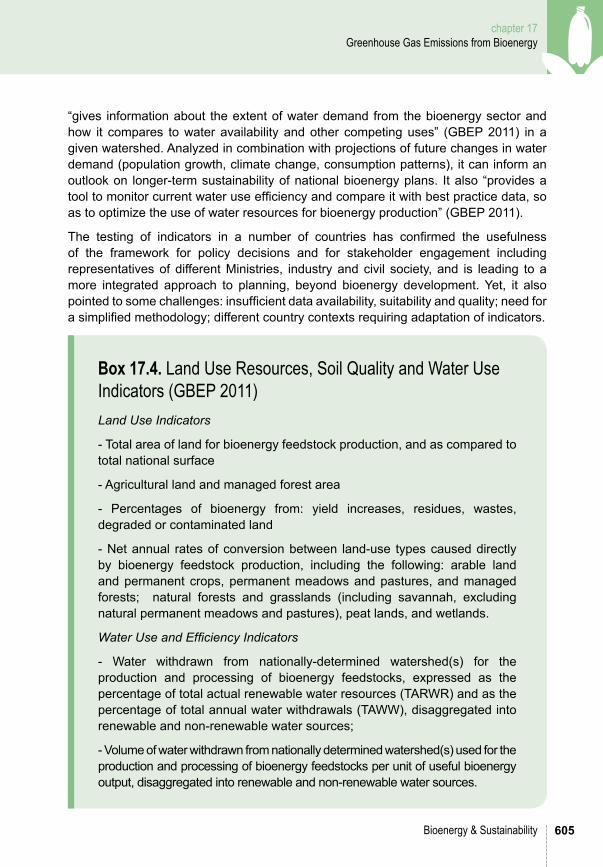
The Global Bioenergy Partnership (GBEP 2011) agreed on 24 sustainability indicators to provide a framework for collecting data. The indicators are value neutral, “do not feature directions, thresholds or limits and do not constitute a standard, nor are they legally binding. Measured over time, these indicators will show progress towards or away from a nationally-defined sustainable development path” (GBEP 2011), and inform any corrective measures. For example, the four components of the indicator ‘Land use’ (Box 17.4) allow an evaluation of the role bioenergy plays in land use and LUC, and the LUC implications of different bioenergy feedstocks. With the “measurement of the share of land used for bioenergy feedstock that has been subject to some land suitability assessment, it will indicate how bioenergy expansion is part of official land use planning” (GBEP 2011). The indicator on Water use and efficiency (Box 17.4)

Box 17.3. Advanced bioenergy systems may reduce emissions of black carbon and aerosolsBlack carbon emitted through incomplete combustion of biomass is a short-lived but powerful climate forcing agent: it absorbs radiation, influences cloud formation, and when deposited on snow and ice it reduces albedo (Forster et al. 2007). The net effect is complex and site dependent; so there is high uncertainty over the absolute estimates of the impact of black carbon. Organic carbon particles released through biomass combustion scatter radiation, offsetting global warming caused by black carbon (Forster et al. 2007). Increased use of bioenergy in developed countries may increase emissions of black carbon and organic carbon; but replacing traditional fuel wood uses in developing countries with improved biomass cook stoves and advanced bioenergy technologies is critical to reducing black carbon emissions (UNEP 2011).

605



“gives information about the extent of water demand from the bioenergy sector and how it compares to water availability and other competing uses” (GBEP 2011) in a given watershed. Analyzed in combination with projections of future changes in water demand (population growth, climate change, consumption patterns), it can inform an outlook on longer-term sustainability of national bioenergy plans. It also “provides a tool to monitor current water use efficiency and compare it with best practice data, so as to optimize the use of water resources for bioenergy production” (GBEP 2011).

The testing of indicators in a number of countries has confirmed the usefulness of the framework for policy decisions and for stakeholder engagement including representatives of different Ministries, industry and civil society, and is leading to a more integrated approach to planning, beyond bioenergy development. Yet, it also pointed to some challenges: insufficient data availability, suitability and quality; need for a simplified methodology; different country contexts requiring adaptation of indicators.

Box 17.4. land Use Resources, Soil Quality and Water Use Indicators (gBEP 2011)Land Use Indicators

- Total area of land for bioenergy feedstock production, and as compared to total national surface

- Agricultural land and managed forest area

- Percentages of bioenergy from: yield increases, residues, wastes, degraded or contaminated land

- Net annual rates of conversion between land-use types caused directly by bioenergy feedstock production, including the following: arable land and permanent crops, permanent meadows and pastures, and managed forests; natural forests and grasslands (including savannah, excluding natural permanent meadows and pastures), peat lands, and wetlands.

Water Use and Efficiency Indicators

- Water withdrawn from nationally-determined watershed(s) for the production and processing of bioenergy feedstocks, expressed as the percentage of total actual renewable water resources (TARWR) and as the percentage of total annual water withdrawals (TAWW), disaggregated into renewable and non-renewable water sources;

- Volume of water withdrawn from nationally determined watershed(s) used for the production and processing of bioenergy feedstocks per unit of useful bioenergy output, disaggregated into renewable and non-renewable water sources.

606



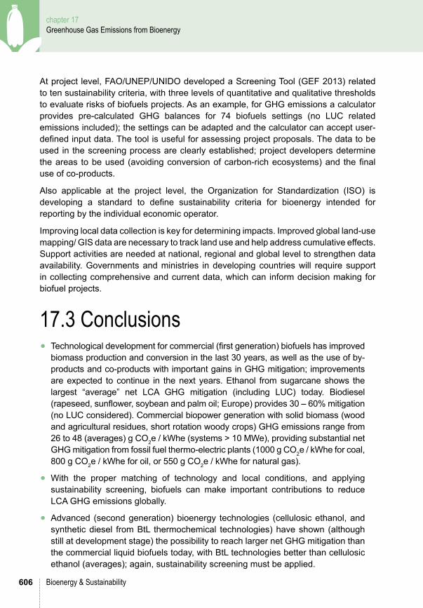
At project level, FAO/UNEP/UNIDO developed a Screening Tool (GEF 2013) related to ten sustainability criteria, with three levels of quantitative and qualitative thresholds to evaluate risks of biofuels projects. As an example, for GHG emissions a calculator provides pre-calculated GHG balances for 74 biofuels settings (no LUC related emissions included); the settings can be adapted and the calculator can accept user-defined input data. The tool is useful for assessing project proposals. The data to be used in the screening process are clearly established; project developers determine the areas to be used (avoiding conversion of carbon-rich ecosystems) and the final use of co-products.

Also applicable at the project level, the Organization for Standardization (ISO) is developing a standard to define sustainability criteria for bioenergy intended for reporting by the individual economic operator.

Improving local data collection is key for determining impacts. Improved global land-use mapping/ GIS data are necessary to track land use and help address cumulative effects. Support activities are needed at national, regional and global level to strengthen data availability. Governments and ministries in developing countries will require support in collecting comprehensive and current data, which can inform decision making for biofuel projects.

17.3 Conclusions ● Technological development for commercial (first generation) biofuels has improved

biomass production and conversion in the last 30 years, as well as the use of by-products and co-products with important gains in GHG mitigation; improvements are expected to continue in the next years. Ethanol from sugarcane shows the largest “average” net LCA GHG mitigation (including LUC) today. Biodiesel (rapeseed, sunflower, soybean and palm oil; Europe) provides 30 – 60% mitigation (no LUC considered). Commercial biopower generation with solid biomass (wood and agricultural residues, short rotation woody crops) GHG emissions range from 26 to 48 (averages) g CO2e / kWhe (systems > 10 MWe), providing substantial net GHG mitigation from fossil fuel thermo-electric plants (1000 g CO2e / kWhe for coal, 800 g CO2e / kWhe for oil, or 550 g CO2e / kWhe for natural gas).

● With the proper matching of technology and local conditions, and applying sustainability screening, biofuels can make important contributions to reduce LCA GHG emissions globally.

● Advanced (second generation) bioenergy technologies (cellulosic ethanol, and synthetic diesel from BtL thermochemical technologies) have shown (although still at development stage) the possibility to reach larger net GHG mitigation than the commercial liquid biofuels today, with BtL technologies better than cellulosic ethanol (averages); again, sustainability screening must be applied.

607



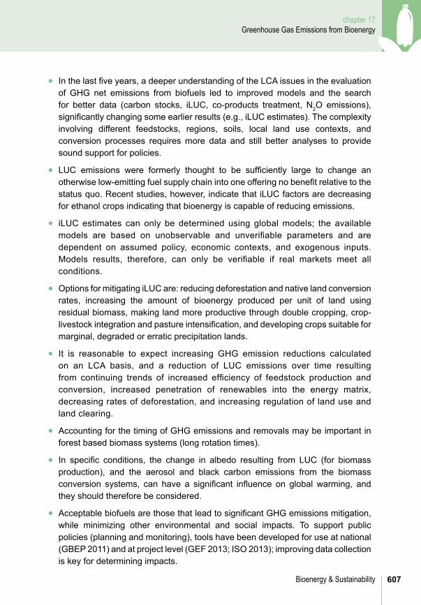
● In the last five years, a deeper understanding of the LCA issues in the evaluation of GHG net emissions from biofuels led to improved models and the search for better data (carbon stocks, iLUC, co-products treatment, N2O emissions), significantly changing some earlier results (e.g., iLUC estimates). The complexity involving different feedstocks, regions, soils, local land use contexts, and conversion processes requires more data and still better analyses to provide sound support for policies.

● LUC emissions were formerly thought to be sufficiently large to change an otherwise low-emitting fuel supply chain into one offering no benefit relative to the status quo. Recent studies, however, indicate that iLUC factors are decreasing for ethanol crops indicating that bioenergy is capable of reducing emissions.

● iLUC estimates can only be determined using global models; the available models are based on unobservable and unverifiable parameters and are dependent on assumed policy, economic contexts, and exogenous inputs. Models results, therefore, can only be verifiable if real markets meet all conditions.

● Options for mitigating iLUC are: reducing deforestation and native land conversion rates, increasing the amount of bioenergy produced per unit of land using residual biomass, making land more productive through double cropping, crop-livestock integration and pasture intensification, and developing crops suitable for marginal, degraded or erratic precipitation lands.

● It is reasonable to expect increasing GHG emission reductions calculated on an LCA basis, and a reduction of LUC emissions over time resulting from continuing trends of increased efficiency of feedstock production and conversion, increased penetration of renewables into the energy matrix, decreasing rates of deforestation, and increasing regulation of land use and land clearing.

● Accounting for the timing of GHG emissions and removals may be important in forest based biomass systems (long rotation times).

● In specific conditions, the change in albedo resulting from LUC (for biomass production), and the aerosol and black carbon emissions from the biomass conversion systems, can have a significant influence on global warming, and they should therefore be considered.

● Acceptable biofuels are those that lead to significant GHG emissions mitigation, while minimizing other environmental and social impacts. To support public policies (planning and monitoring), tools have been developed for use at national (GBEP 2011) and at project level (GEF 2013; ISO 2013); improving data collection is key for determining impacts.

608



17.4 Recommendations The experience with commercial biofuels development, the successful results (aiming at GHG emissions mitigation), the great improvements in co- and by-product utilization, and the potential for advanced biofuels indicate the paths to follow towards more efficient and sustainable biofuels. Technical challenges include methodological difficulties in evaluating GHG emissions, and the need for reliable data. Institutional challenges include support for implementing adequate policies. To address the needs, we recommend:

● Support programs to improve local data for soil conditions, SOM stock changes, and N2O emissions; and to improve the knowledge of the impacts on climate of timing of GHG emissions and removals, and of biomass production / conversion (processes that affect albedo and aerosols).

● Continued efforts towards harmonization in outstanding GHG quantification issues (by-products, co-products and residues treatment; iLUC consideration and interpretation).

● Actions are needed both at national policy and at project levels to enhance GHG benefits from biofuels. The main points are: establishing of specific zoning systems to manage LUC emissions; policies for deforestation control and monitoring; implementation of good practices in agriculture and forestry; programs for increasing land productivity (see Chapter 9, this volume). New governance structures supported by technical understanding and effective monitoring may be needed. Bioenergy could lead the development of such structures, with benefits that would spill over the whole (much larger) land use sector, including agriculture and forestry.

17.5 The much Needed Science ● New technologies for advanced biofuels production;

● Search for a higher level of (scientific) consensus on the treatment of net emissions for co-products and by-products;

● N2O emissions data in bioenergy systems;

● Local data on SOM change with LUC;

● Search for a higher level of (scientific) consensus on the iLUC evaluation;

● Global land use data and monitoring system (including agriculture, silviculture, and pastures); see Chapter 16, this volume.

609



literature CitedAl-Riffai, P, Dimaranan, B and Laborde, D 2010. Global Trade and Environmental Impact Study of

the EU Biofuels Mandate. Specific Contract No SI2.537.787 implementing Framework Contract No TRADE/07/A2, Final report March 2010.

Arima, E.Y., Richards, P., Walker, R., Caldas, M.M., 2011. Statistical confirmation of indirect land use change in the Brazilian Amazon. Environmental Research Letters 6.

Barona, E., Ramankutty, N., Hyman, G., Coomes, O.T., 2010. The role of pasture and soybean in deforestation of the Brazilian Amazon. Environmental Research Letters 5.

Bauen A., Chudziak C.,Vad K.,Watson P., 2010. A causal-descriptive approach to modelling the GHG emissions associated with the indirect land-use impacts of biofuels. A study for the UK Department for Transport, E4tech.

Berndes, G., Bird, N., Cowie, A. 2010. Bioenergy, land use change and climate change mitigation: Report for policy advisors and policy makers. IEA Bioenergy:ExCo:2010:03

BioGrace 2013. Available at: http://www.biograce.net/home - accessed September 2014

Borrion AL, McManus MC, Hammond GP, 2012. Environmental life cycle assessment of lignocellulosic conversion to ethanol: A review. Renewable and Sustainable Energy Reviews 2012;16:4638–50.

Brandão M, Levasseur A, Kirschbaum MUF, Weidema BP, Cowie AL, Jørgensen SV, Hauschild MZ, Pennington DW & Chomkhamsri K 2012 Key issues and options in accounting for carbon sequestration and temporary storage in life cycle assessment and carbon footprinting. Int J Life Cycle Assess 18:230-240.

Brander, M., Tipper, R., Hutchison, C., Davis, G. 2009. Consequential and Attributional Approaches to LCA: a Guide to Policy Makers with Specific Reference to Greenhouse Gas LCA of Biofuels. Econometrica Press: April 2008.

Bright RM, Astrup R and Strømman AH. 2013. Empirical models of monthly and annual albedo in managed boreal forests of interior Norway. Climatic Change September, Volume 120, Issue 1-2, pp 183-196.

Bright RM, Strømman AH and Peters GP 2011 Radiative Forcing Impacts of Boreal Forest Biofuels: A Scenario Study for Norway in Light of Albedo Environ. Sci. Technol. 45, 7570–7580

Bruckner, T., Chum, H., Jäger-Waldau, A., Killingtveit, Å., Gutiérrez-Negrín, L., Nyboer, J., Musial, W., Verbruggen, A., Wiser, R. 2011. Annex III: Cost Table. In Edenhofer, O., Pichs-Madruga, R., Sokona, Y., Seyboth, K., Matschoss, P., Kadner, S., Zwickel, T., Eickemeier, P., Hansen, G., Schlömer, S., von Stechow, C. (eds) IPCC Special Report on Renewable Energy Sources and Climate Change Mitigation, Cambridge University Press, Cambridge, United Kingdom and New York, NY, USA.

CARB 2009. CARB Staff Report: Proposed Regulation to Implement the Low Carbon Fuel Standard. California Air Resources Board: March 5, 2009.

CARB 2009. CARB Staff Report: Proposed Regulation to Implement the Low Carbon Fuel Standard. California Air Resources Board: March,, 2009.

CARB 2014. iLUC Analysis for the Low Carbon Fuel Standard (Update). California Air Resources Board: March, 2014.

Cherubini F et al 2013 Global climate impacts of forest bioenergy: what, when and how to measure? Environ. Res. Lett. 8 014049

http://www.biograce.net/home

http://link.springer.com/journal/10584

http://link.springer.com/journal/10584/120/1/page/1

http://iopscience.iop.org/1748-9326/8/1/014049

610



Cowie AL, Berndes, G and Smith CT 2013 On the timing of Greenhouse Gas Mitigation Benefits of Forest-Based Bioenergy. IEA Bioenergy ExCo 2013:04 http://www.ieabioenergy.com/wp-content/uploads/2013/10/On-the-Timing-of-Greenhouse-Gas-Mitigation-Benefits-of-Forest-Based-Bioenergy.pdf - accessed September 2014

Cherubini F, Bird ND, Cowie A, Jungmeier G, Schlamadinger B, Woess-Gallasch S.2009. Energy- and greenhouse gas-based LCA of biofuel and bioenergy systems: Key issues, ranges and recommendations. Resources, Conservation and Recycling 2009;53:434–47

Cherubini, Bright RM and Strømman AH 2012 Site-specific global warming potentials of biogenic CO2 for bioenergy: contributions from carbon fluxes and albedo dynamics. Environ. Res. Lett. 7 (2012) 045902 (11pp)

Cherubini, F., G. B. Peters, T. Bernsten, A. H. Strømman, and E. Hertwich. 2011. CO2 emissions from biomass combustion for bioenergy: Atmospheric decay and contribution to global warming. GCB Bioenergy 3(5): 413–426.

Chum, H.L., Warner, E., Seabra, J.E.A., Macedo I.C. 2013a. A comparison of commercial ethanol production systems from Brazilian sugarcane and U.S. corn. Biofuels Bioproducts & Biorefining. doi:10.1002bbb.1448.

Chum, H.L., Zhang, Y., Hill, J., Tiffany, D.G., Morey, R.V., Eng, A.G., Haq, Z. 2013b. Understanding the evolution of environmental and energy performance of the U.S. corn ethanol industry: evaluation of selected metrics. Biofuels Bioproducts & Biorefing, doi:10.1002/bbb.1449.

Delucchi, M. 2003. A Lifecycle Emissions Model (LEM): Lifecycle Emissions from Transportation Fuels, Motor Vehicles, Transportation Modes, Electricity Use, Heating and Cooking Fuels, and Materials. Report UCD-ITS-RR-03-17. Davis, California.

Dunn, J. B.; Mueller, S.; Kwon, H,; Wang, M. Q. 2013. Land-use change and greenhouse gas emissions from corn and cellulosic ethanol. Biotechnology for Biofuels 2013, 6:51. (doi:10.1186/1754-6834-6-51).

E4Tech 2010. A Causal Descriptive Approach to Modeling the GHG Emissions Associated with the Indirect Land Use Impacts of Biofuels. Final report. A study for the UK Department for Transport, October 2010.

EC 2009. Directive 2009/28/EC of the European Parliament and of the Council of 23 April 2009 on the promotion of the use of energy from renewable sources and amending and subsequently repealing Directives 2001/77/EC and 2003/ 30/EC.

EC 2010. European Commission decision of 10 June 2010 on guidelines for the calculation of land carbon stocks for the purpose of Annex V to Directive 2009/28/EC. In: Official Journal of the European Union, L151/19-41, 2010

Ecoinvent 2013. Ecoinvent database, Swiss Centre for Life Cycle Inventories. http://www.ecoinvent.ch/ - accessed September 2014

Edwards, R., Larivé, J.F., Rickeard, D., Weindorf, W. 2013. Well-to-tank report version 4.0, JEC Well-to-Wheels Analysis of Future Automotive Fuels and Powertrains in the European Context, Italy, doi:10.2788/40526.

ELCD 2013. European reference Life Cycle Database. Available at: http://lct.jrc.ec.europa.eu/assessment/data Accessed October 17, 2013.

Elliot, J.; Sharma, B.; Best, N.; Glotter, M.; Dunn, J. B.; Foster, I.; Miguez, F.; Mueller, S.; Wang, M. A Spatial Modeling Framework to Evaluate Domestic Biofuel-Induced Potential Land Use Changes and Emissions. Environmental Science and Technology, 2014, 48 (4), pp 2488–2496 (DOI: 10.1021/es404546r).

http://www.ieabioenergy.com/wp-content/uploads/2013/10/On-the-Timing-of-Greenhouse-Gas-Mitigation-Benefits-of-Forest-Based-Bioenergy.pdf

http://www.ieabioenergy.com/wp-content/uploads/2013/10/On-the-Timing-of-Greenhouse-Gas-Mitigation-Benefits-of-Forest-Based-Bioenergy.pdf

http://www.ecoinvent.ch/

http://lct.jrc.ec.europa.eu/assessment/data

http://lct.jrc.ec.europa.eu/assessment/data

611



Elobeid, A.; Carriquiry, M.; Fabiosa, J. F. 2011. Global Biofuel Expansion and the Demand for Brazilian Land: Intensification versus Expansion. Selected Paper prepared for presentation at the Agricultural and Applied Economics Association’s 2011 AAEA & NAREA Joint Annual Meeting, Pittsburg, Pennsylvania, July 24-26, 2011.

EPA 2010. Renewable Fuel Standard Program (RFS2) Regulatory Impact Analysis. Assessment and Standards Division, Office of Transportation and Air Quality, U.S. Environmental Protection Agency: February, 2010.

FAO/IIASA/ISRIC/ISS-CAS/JRC 2008. Harmonized World Soil Database (version 1.0). FAO, Rome, Italy and IIASA, Laxenburg, Austria.

Farrell, A.E., Plevin, R.J., Turner, B.T., Jones, A.D., O’Hare, M., Kammen, D.M. 2006. Ethanol can contribute to energy and environmental goals. Science 311: 506-508.

Finnveden, G., Hauschild, M.Z., Ekvall, T., Guinée, J., Heijungs, R., Hellweg, S., Koehler, A., Pennington, D., Suh, S. 2009. Recent developments in Life Cycle Assessment. Journal of Environmental Management 91:1-21.

Forster, P., V. Ramaswamy, P. Artaxo, T. Berntsen, R. Betts, D.W. Fahey, J. Haywood, J. Lean, D.C. Lowe, G. Myhre, J. Nganga, R. Prinn, G. Raga, M. Schulz and R. Van Dorland, 2007: Changes in Atmospheric Constituents and in Radiative Forcing. In: Climate Change 2007: The Physical Science Basis. Contribution of Working Group I to the Fourth Assessment Report of the Intergovernmental Panel on Climate Change [Solomon, S., D. Qin, M. Manning, Z. Chen, M. Marquis, K.B. Averyt, M.Tignor and H.L. Miller (eds.)]. Cambridge University Press, Cambridge, United Kingdom and New York, NY, USA.

Fritsche U, Hennenberg K, Hunecke K. 2010. The ‘iLUC Factor’ as a Means to Hedge Risks of GHG Emissions from Indirect Land Use Change. Darmstadt: Oeko Institute.

GaBi 2013. GaBi Software, PE International. http://www.gabi-software.com/index/ - accessed September 2014

Galdos, M.V. et al. 2009. Simulation of Soil Carbon Dynamics under Sugarcane with the CENTURY Model. Science Society of America Journal Vol. 73 No. 3, p. 802-811

Gao, Y, Skutsch, O., Masera, o, Pacheco, P. 2011. A global analysis of deforestation due to biofuel development. Working Paper 68. CIFOR. Available at: http://www.cifor.org/publications/pdf_files/WPapers/WP68Pacheco.pdf - accessed September 2014

GBEP 2011. The Global Bioenergy Partnership. Sustainability Indicators for Bioenergy, 2011. http://www.globalbioenergy.org/?id=25880 - accessed September 2014

GEF Targeted Project 2013. Global Assessment and Guidelines for Sustainable Liquid Biofuel Production in developing Countries.

Georgescu M, Lobell DB, Field CB. 2011. Direct climate effects of perennial bioenergy crops in the United States. Proc Natl Acad Sci U S A, 108:4307– 4312.

GHG Protocol 2011. Product Life Cycle Accounting and Reporting Standard. World Resources Institute and World, Business Council for Sustainable Development.

Gnansounou E, Dauriat A, Villegas J, Panichelli L. 2009. Life cycle assessment of biofuels: energy and greenhouse gas balances. Bioresource Technology 2009;100:4919–30.

GREET 2012. The Greenhouse Gases, Regulated Emissions, and Energy Use in Transportation (GREET) Model. Available at: http://greet.es.anl.gov/main - accessed September 2014

GREET1 2013. GREET Model: The Greenhouse Gases, Regulated Emissions, and Energy Use in Transportation Model. Argonne National Laboratory.

http://www.gabi-software.com/index/

http://www.cifor.org/publications/pdf_files/WPapers/WP68Pacheco.pdf

http://www.globalbioenergy.org/?id=25880

http://greet.es.anl.gov/main

612



Guest, G., Cherubini, F., Strømman, A.H. 2013. Global Warming Potential of Carbon Dioxide Emissions from Biomass Stored in the Anthroposphere and Used for Bioenergy at End of Life Journal of Industrial Ecology, 17 (1), pp. 20-30.

Harfuch, L.; Bachion, L.C.; Moreira M.M.R.; Nassar, A.M.; Carriquiry, M. 2014. Agricultural Expansion and Land Use Changes in Brazil: Using Empirical Evidence. In: Handbook of Bioenergy Economics and Policy (in press). Springer

Havlik, P.; Valin, H.; Mosnier, A.; Obersteiner, M.; Baker, J. S.; Herrero, M.; Rufino, M. C.; Schmid, E. 2013. Crop productivity and the global livestock sector: Implications for land use change and greenhouse gas emissions. American Journal of Agricultural Economics, 95(2):442-448 (http://dx.doi.org/10.1093/ajae/aas085).

Hertel, T. W. , S. Rose, and R. Tol. 2009. “Land Use in Computable General Equilibrium Models: An Overview.” In Economic Analysis of Land Use in Global Climate Change Policy, edited by T.W. Hertel, S. Rose and R. Tol. UK: Routledge Press.

Hertel, T.; Golub, A. A.; Jones, A. D; O’Hare M.; Plevin, R. J.; Kammen, D. M. Global land use and greenhouse gas emissions impacts of U.S. maize ethanol: estimating market mediated responses. Biosci. 2010, 60 (3), 223–231; DOI: 10.1525/bio.2010.60.3.8.

Hertel, Thomas W. , ed. 1997. Global Trade Analysis: Modeling and Applications. New York: Cambridge University Press.

Hertel, Thomas W., and Wallace E. Tyner. 2013. “Market-mediated environmental impacts of biofuels.” Global Food Security no. 2:131-37.

Hertel, Thomas W., W.E. Tyner, and Dileep K. Birur. 2010. “The Global Impacts of Biofuel Mandates.” The Energy Journal no. 30 (1):75-100.

Hudiburg T., Law B.E., Wirth C., Luyssaert S. 2011. Regional carbon dioxide implications of forest bioenergy production. Nature Climate Change, 1, 419-423.

Huo, H., Wang, M., Bloyd, C., Putsche, V. 2009. Life-Cycle Assessment of Energy and Greenhouse Gas Effects of Soybean-Derived Biodiesel and Renewable Fuels. Environmental Science & Technology 43:750-756.

IEA Bioenergy 2010. Minutes of the workshop State of the art technologies for small biomass co-generation. International Energy Agency Bioenergy Agreement Task 32, Joint workshop with Task 33. 7 October, 2010, Copenhagen, Denmark.

ILCD 2010. ILCD Handbook: General guide for Life Cycle Assessment – Detailed guidance. Joint Research Centre, Institute for Environment and Sustainability.

IPCC 2006. IPCC Guidelines for National Greenhouse Gas Inventories. The National Greenhouse Gas Inventories Programme, The Intergovernmental Panel on Climate Change, H.S. Eggleston, L. Buendia, K. Miwa, T. Ngara, and K. Tanabe (eds.). Hayama, Kanagawa, Japan.IRP Land Report 2013. Assessing Global Land Use: Balancing Consumption with Sustainable Supply, UNEP 2013

ISO 2006a. ISO 14040:2006(E), Environmental management – Life cycle assessment – Principles and framework.

ISO 2006b. ISO 14044:2006(E), Environmental management – Life cycle assessment – Requirements and guidelines.

ISO 2006c. ISO 14041:2006, Procedure, clause 6.5.3.

ISO 2013. ISO/TS:2013(E), Greenhouse gases – Carbon footprint of products – Requirements and guidelines for quantification and communication.

613



ISO/CD 13065 2013. Sustainability criteria for bioenergy. http://www.iso.org/iso/catalogue_detail?csnumber=52528 - accessed September 2014

JRC 2010a. Carré F., R. Hiederer, V. Blujdea, R. Koeble. Background guide for the calculation of land carbon stocks in the biofuels sustainability scheme: drawing on the 2006 IPCC guidelines for national greenhouse gas inventories; Joint Research Centre of European Commission. EUR 24573 EN, 2010; http://eusoils.jrc.ec.europa.eu/ESDB_Archive/eusoils_docs/other/EUR24573.pdf - accessed September 2014

JRC 2010b. Hiederer R., F. Ramos , C. Capitani, R. Koeble, V. Blujdea, O. Gomez, D. Mulligan and L. Marelli. Biofuels: a New Methodology to Estimate GHG Emissions Due to Global Land Use Change. JRC Scientific and Technical Reports: EUR 24483 EN, 2010. Available at http://iet.jrc.ec.europa.eu/bf-ca/publications - accessed September 2014

JRC 2011. Marelli, L., F. Ramos, R. Hiederer and R. Koeble. Estimate of GHG emissions from global land use change scenarios. Joint Research Centre of European Commission. EUR 24817 EN, 2011. Available at http://iet.jrc.ec.europa.eu/bf-ca/publications - accessed September 2014

Keeney, R. and Hertel, T.W. 2009. The indirect land use impacts of United States biofuel policies: The importance of acreage, yield, and bilateral trade responses, American Journal of Agricultural Economics 91(4): 895-909

Khanna, M and Crago C.L. 2012. Measuring Indirect Land Use Change with Biofuels: Implications for Policy, Annual Review of Resource Economics, 4: DOI: 10.1146/annurev-resource-110811-114523

Khatiwada, D., Seabra, J., Silveira, S., Walter, A. 2012. Accounting greenhouse gas emissions in the lifecycle of Brazilian sugarcane bioethanol: Methodological references in European and American regulations. Energy Policy 47:384-397.

Kim, S., Dale, B.E. 2008. Life cycle assessment of fuel ethanol derived from corn grain via dry milling. Bioresource Technology 99: 5250-5260.

Kim, S., Dale, B.E., 2009. Regional variations in greenhouse gas emissions of biobased products in the United States-corn-based ethanol and soybean oil. International Journal of Life Cycle Assessment 14, 540-546

Kretschmer B, Peterson S. Integrating bioenergy into computable general equilibrium models – a survey. Energy Econ 2010(32): 673-686

Laborde, D. 2011. Assessing the Land Use Change Consequences of European Biofuel Policies. Final Report, IFPRI, October 2011.

Laborde, D.; Padella, M.; Edwards, R.; Marelli, L. 2014 Progress in Estimates of iLUC with Mirage Model. Joint Research Center, Report EUR 26106 EN.

Lapola, D.M., Schaldach, R., Alcamo, J., Bondeau, A., Koch, J., Koelking, C., Priess, J.A.,2010. Indirect land-use changes can overcome carbon savings from biofuels in Brazil. Proc. Natl. Acad. Sci. USA. (doi/10.1073/pnas.0907318107)

LBSM 2013. Ludwig-Bölkow-Systemtechnik-GMBH (LBSM) E3 database. http://www.e3database.com/ - accessed September 2014

Levasseur, A., P. Lesage, M. Margni, L. Deschenes, and R. Samson. 2010. Considering time in LCA: Dynamic LCA and its application to global warming impact assessments. Environmental Science and Technology 44(8): 3169–3174.

Loarie S R, Lobel DB, Asner GP, Mu Q, Field CB. 2011. Direct impacts on local climate of sugar-cane expansion in Brazil. Nat Climate Change 2011, 1:105–109.

Macedo, I.C., Seabra, J.E.A., Silva, J.E.A.R. 2008. Green house gas emissions in the production and use of ethanol from sugarcane in Brazil: the 2005/2006 averages with a prediction of 2020. Biomass and Bioenergy 32: 582-595.

http://www.iso.org/iso/catalogue_detail?csnumber=52528

http://www.iso.org/iso/catalogue_detail?csnumber=52528

http://eusoils.jrc.ec.europa.eu/ESDB_Archive/eusoils_docs/other/EUR24573.pdf

http://www.e3database.com/

614



Marelli, L.; Ramos, F.; Hiederer, R.; Koeble, R. 2011 Estimate of GHG emissions from global land use change scenarios. JRC Technical Notes. EUR 24817 EN - 2011

Mathews, J., Tan, H. 2009. Biofuels and indirect land use change effects: the debate continues. Biofuels, Bioprod. Bioref. DOI: 10.1002/bbb.147

McKechnie J, Colombo S, Cheng J, Mabee W, MacLean HL. 2011. Forest bioenergy or forest carbon? Assessing trade-offs in greenhouse gas mitigation with wood-based fuels. Environmental Science and Technology, 45, 2, 789-95.

Mello, F.C., C. E. P. Cerri, C. A. Davies, N. M. Holbrook, K. Paustian, S. M. F. Maia, M.V. Galdos, M. Bernoux, and Carlos C. Cerri. 2014. Payback time for soil carbon and sugar-cane ethanol. Nature Climate Change, DOI: 10.1038/NCLIMATE2239 June 2014

Menichetti E, O M. 2008. Energy balance and greenhouse gas emissions of biofuels from a life-cycle perspective. In: Howarth RW, Bringezu S, editors. Biofuels: Environmental Consequences and Interactions with Changing Land Use. Proceedings of the Scientific Committee on Problems of the Environment (SCOPE) International Biofuels Project Rapid Assessment, Ithaca NY: University of Cornell; 2008, p. 81–109

Menten, F., Chèze, B., Patouillard, L., Bouvart, F. 2013. A review of LCA greenhouse gas emissions results for advanced biofuels: The use of meta-regression analysis. Renewable and Sustainable Energy Reviews 26: 108-134.

Moreira, M.; Nassar, A.; Antoniazzi, L.; Bachion, L. C.; Harfuch, L. 2012. Direct and indirect land use change assessment. In: Poppe, M. K.; Cortez, L. A. B. Sustainability of sugarcane bioenergy. Center for Strategic Studies and Management (CGEE), 2012.

Mueller, S. 2010. 2008 national dry mill corn ethanol survey. Biotechnology Letters (May), doi:10.1007/s10529-010-0296-7.

Nassar, A. M.; Harfuch L.; Bachion, L. C.; Moreira M. M. R. 2011 “Biofuels and land-use changes: searching for the top model.” Interface Focus 1 (2): 224–232. (doi:10.1098/rsfs.2010.0043)

NREL, 2013. Energy Analysis: International Trade of Wood Pellets. NREL/BR-6A20-56791, May 2013. http://www.nrel.gov/docs/fy13osti/56791.pdf - accessed September 2014

PAS 2050 2011. PAS 2050:2011, Specification for the assessment of the life cycle greenhouse gas emissions of goods and services.

Plevin, R. H. K. Gibbs, J. Duffy, S. Yeh, and S. Yui. 2011. Updated Emissions Factor Model for GTAP. Report for the California Air Resources Board

Pradham, A., Shrestha, D.S., Van Gerpen, J., McAloon, A., Yee, W., Hass, M., Duffield, J.A. 2012. Reassessment of life cycle greenhouse gas emissions for soybean biodiesel. Transactions of teh American Socieity of Agricultural and Biological Engineers 55(6): 2257-2264.

Prins, A., Stehfest, E., Overmars, K., and Ros, J. 2010. Are models suitable for determining iluc factors? Bilthoven: Netherlands Environmental Assessment Agency. Publication number 500143006. Available at: http://www.pbl.nl/en

RSB 2011. RSB GHG Calculation Methodology. RSB reference code: RSB-STD-01-003-01 (Version 2.0). Roundtable on Sustainable Biofuels.

Schwaiger HP and Bird DN 2010). Integration of albedo effects caused by land use change into the climate balance: Should we still account in greenhouse gas units? Forest Ecology and Management 260, 278-286

SCOPE 2009. Biofuels: Environmental Consequences and Interactions with Changing Land Use, edited by R.W. Howarth and S. Bringezu. Proceedings of the Scientific Committee on Problems of the Environment (SCOPE) International Biofuels Project Rapid Assessment. 22-25 September 2008. Gummersbach, Germany

http://www.nrel.gov/docs/fy13osti/56791.pdf

615



Seabra J.E.A., Macedo, I.C., Chum, H.L., Faroni, C.E., Sarto, C.A. 2011. Life cycle assessment of Brazilian sugarcane products: GHG emissions and energy use. Biofuels, Bioproducts and Biorefining 5: 519–32.

Searchinger, T.; Heimlich, R.; Houghton R. A.; Dong, F.; Elobeid, A.; Fabiosa J. Use of U.S. croplands for biofuels increases greenhouse gases through emissions from land-use change. Science v. 319, p. 1238–1240. 2008.

Sheehan, J., Camobreco, V., Duffield, J., Graboski, M., Shapouri, M. 1998. Life-cycle inventory of biodiesel and petroleum diesel for use in an urban bus, prepared for U.S. Department of Energy, Office of Fuels Development, Washington, D.C.

SimaPro 2013. SimaPro LCA Software, PRé. http://www.pre-sustainability.com/ - accessed September 2014

Taheripour, F., Thomas W. Hertel, W.E. Tyner, Jason Beckman, and Dileep K. Birur. 2010. “Biofuels and their by-products: Globla economic and environmental implications.” Biomass and Bioenergy no. 34 (3):278-289.

Taheripour, Farzad, and Wallace E. Tyner. 2013. “Biofuels and Land Use Change: Applying Recent Evidence to Model Estimates” Applied Sciences no. 3:14-38.

Taheripour, Farzad, Qianlai Zhuang, Wallace E. Tyner, and Xiaoliang Lu. 2012. “Biofuels, cropland expansion, and the extensive margin.” Energy, Sustainability and Society no. 2 (25).

Taheripour, Farzad, T. W. Hertel, and Wallace E. Tyner. 2011. “Implications of biofuels mandates for the global livestock industry: a computable general equilibrium analysis.” Agricultural Economics no. 42:325–342.

Tipper R, Hutchison C, Brander M. 2009. A Practical Approach for Policies to Address GHG Emissions from Indirect Land Use Change Associated with Biofuels. Technical Paper - TP- 080212-A. Ecometrica and Greenenergy

Tyner, W. E.; Taheripour, F.; Zhuang, Q.; Birur, D.; Baldos, U. Land use changes and consequent CO2 emissions due to U.S. corn ethanol production: a comprehensive analysis; Purdue University, West Lafayette, Indiana, 2010; https://www.gtap.agecon.purdue.edu/resources/download/5200.pdf - accessed September 2014

Umberto 2013. Umberto NXT LCA, ifu Hamburg. http://www.umberto.de/en/ - accessed September 2014

UNEP 2010. Bioenergy Issue Paper Series no.1; Land Use, Land Use Change and Bioenergy . http://www.unep.org/bioenergy/Portals/48107/doc/issues/issuespaper/Issue%20Paper%201.pdf - accessed September 2014

UNEP 2011. Near-term Climate Protection and Clean Air Benefits: Actions for Controlling Short-Lived Climate Forcers, United Nations Environment Programme (UNEP), Nairobi, Kenya, 78pp

UNEP GEOS-5 2012. The Fifth Global Environmental Outlook, UNEP, 2012

Walker, T., Cardellichio, P., Colnes, A., Gunn, J., Kittler, B., Perschel, R., Recchia, C., Saah, D., 2010. Biomass Sustainability and Carbon Policy Study: Report to the Commonwealth of Massachusetts Department of Energy Resources. Manomet Center for Conservation Sciences. Report No.: NCI-2010-03.

Wang, M., Han, J., Dunn, J., Cai, H., Elgowainy, A. 2012. Well-to-Wheels Energy Use and Greenhouse Gas Emissions of Ethanol from Corn, Sugarcane, Corn Stover, Switchgrass, and Miscanthus. Environmental Research Letters, 7, 045905 (13pp).

Wang, M., Han, J., Haq, Z., Tyner, W., Wu, M., Elgowainy, A. 2011b. Energy and Greenhouse Gas Emission Effects of Corn and Cellulosic Ethanol with Technology Improvements and Land Use Changes. Biomass and Bioenergy 35: 1885-1896.

https://www.gtap.agecon.purdue.edu/resources/download/5200.pdf

http://www.unep.org/bioenergy/Portals/48107/doc/issues/issuespaper/Issue%20Paper%201.pdf

616



Wang, M., Huo, H., Arora, S. 2011a. Methodologies of Dealing with Co-Products of Biofuels in Life-Cycle Analysis and Consequent Results within the U.S. Context. Energy Policy 39: 5726-5736.

Wang, M., Wu, M., Hong, H. 2007. Life-Cycle Energy and Greenhouse Gas Emission Impacts of Different Corn Ethanol Plant Types. Environmental Research Letters 2, 024001 (13 pages).

Wang, M.Q., Saricks, C.L., Wu, M. 1999. Fuel Ethanol Produced from U.S. Midwest Corn: Help or Hindrance to the Vision of Kyoto? Journal of the Air and Waste Management Association 49:756-772.

Warner, E., Mann, M., Heath, G. 2013. Literature Review and Sensitivity Analysis of Biopower Life-Cycle Assessments and Greenhouse Gas Emission. EPRI, Palo Alto, CA.

Weidema, B.P. 1993. Market aspects in product life cycle inventory methodology. Journal of Cleaner Production 1(3-4):161-166.

Weisser, D. 2007. A guide to life-cycle greenhouse gas (GHG) emissions from electric supply Technologies. Energy 32 (2007) 1543–1559.

Wicke, B.; van der Hilst, F.; Daioglou, V.; Banse, M.; Beringer,T.; Gerssen-Gondelach, S.; Heijnen, S.; Karssenberg, D.; Laborde, D., Lippe, M.; van Meijl, H.; Nassar, A.; Powell, J.; Prins, A. G.; Rose, S.; Smeets, E. M. W.; Stehfest, E.; Tyner, W. E.; Verstegen, J. A.; Valin, H.; van Vuuren, D. P., Yeh, S.; Faaij, A. P. C.; 2014. Model collaboration for the improved assessment of biomass supply, demand and impacts. Global Change Biology Bioenergy (doi: 10.1111/gcbb.12176).

Wicke, B.; Verweij, P.; van Meijl, H.; van Vuuren, D. P.; Faaij, A. P. C. 2012. Indirect land use change: review of existing models and strategies for mitigation. Biofuels, 3(1), 2012(doi: 10.4155/BFS.11.154).

Wiloso EI, Heijungs R, De Snoo GR. 2012. LCA of second generation bioethanol: A review and some issues to be resolved for good LCA practice. Renewable and Sustainable Energy Reviews 2012;16:5295–308.

Winrock 2009a. Harris, NL, S. Grimland and S. Brown. 2009. Land Use Change and Emission Factors: Updates since Proposed RFS Rule. Report submitted to EPA.

Winrock 2009b. Winrock Emissons Factors Docket; annex to Winrock 2009

Zamagni, A., Guinée, J., Heijungs, R., Masoni, P., Raggi, A. 2012. Lights and shadows in consequential LCA. International Journal of Life Cycle Assessment 17:904-918.

Documents

greenhouse gas Emissions from - BIOEN FAPESPbioenfapesp.org/scopebioenergy/images/chapters/bioen-scope_chapte… · greenhouse gas Emissions from ... The GHG Protocol Product Standard,