Embed Size (px)
Citation preview
GRAVITY AND MAGNETIC DATA REDUCTION SOFTWARE (GraMag2DCon) FOR SITES
CHARACTERIZATION
NOER EL HIDAYAH ISMAIL
UNIVERSITI SAINS MALAYSIA
2015
ii
GRAVITY AND MAGNETIC DATA REDUCTION SOFTWARE (GraMag2DCon) FOR SITES
CHARACTERIZATION
by
NOER EL HIDAYAH ISMAIL
Thesis submitted in fulfilment of the requirements for the degree of
Doctor of Philosophy
OCTOBER 2015
ii
ACKNOWLEDGEMENT
Alhamdulillah, all praise to Allah SWT for the good health and wellbeing that
were necessary to complete this thesis. My sincerest gratitude to my main supervisor,
Associate Professor Dr. Rosli Saad, for his guide while monitoring and helping me
from beginning till the thesis is completed. Moreover, I would like to thank Professor
Dr. Mohd Mokhtar Saidin and Dr. Nordiana Mohd Muztaza for their ideas and
advices given while preparing this thesis. All of the advices from my supervisors
have been priceless. Loads of thanks go to Mr. Yaakub Othman, Mr. Mydin Jamal,
Mr. Shahil Ahmad Khosaini and Mr. Azmi Abdullah, laboratory assistants, who had
assisted and helped me during data acquisitions. To my colleagues, you guys are the
greatest team and supporters. Thank you all, Nur Azwin Ismail, Andy Anderson
Bery, Nur Aminuda Kamaruddin, Teh Saufia Abu Hasim Ajau’ubi, Khairunnisa’
Mohd Ali, Kiu Yap Chong, Mark Jinmin and Shyeh Sahibul Karamah Masnan. Last
but not the least, my beloved parents who always got my back no matter what my
decision is, Ismail Morad and Rukiah Ramli. Thank you for always trusting this
daughter of yours. Not forgotten to my precious sisters who I look up to and
influenced me whether they realized it or not, Ida Fara Fieza Ismail, Rina Farafienar
Ismail and Noer El Huda Ismail. I love you all and thank you so much for all of the
supports and advices you all have given me. And to whom I did not mention their
names here, whether you involved directly or indirectly, I thank you all. Without all
of you, I won’t be able to finish or even start this journey. Thank you.
Lots of love,
Noer El Hidayah Ismail
iii
TABLE OF CONTENTS
Page
Acknowledgement ii
Table of contents iii
List of Tables vii
List of figures viii
List of symbols xi
List of abbreviations xiii
Abstrak xv
Abstract xvii
CHAPTER 1 INTRODUCTION 1
1.0 Background 1
1.1 Problem statements 6
1.2 Objectives 7
1.3 Significance and novelties 7
1.4 Thesis layout 8
CHAPTER 2 LITERATURE REVIEW 10
2.0 Introduction 10
2.1 Gravity method 11
2.1.1 Basic theory 13
2.1.2 Gravity and rock types 16
iv
2.1.3 Measuring gravity 17
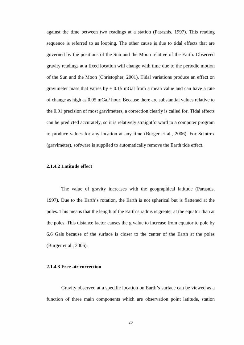
2.1.4 Gravity reduction 18
2.1.4.1 Drift and tidal effect 19
2.1.4.2 Latitude effect 20
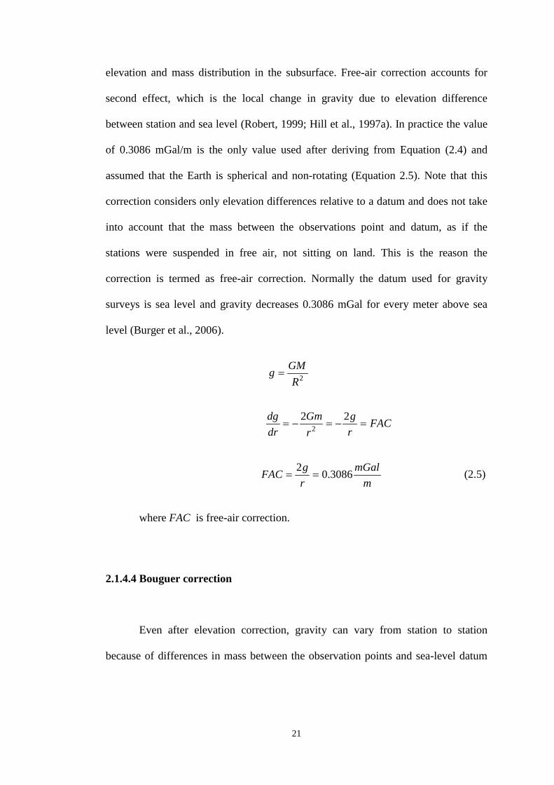
2.1.4.3 Free-air correction 20
2.1.4.4 Bouguer correction 21
2.1.4.5 Terrain correction 23
2.2 Magnetic method 24
2.2.1 Basic Theory 25
2.2.2 Magnetic field 27
2.2.3 Magnetic properties of rocks 28
2.2.4 Measuring magnetic 30
2.2.5 Magnetic reduction/correction 31
2.2.5.1 Diurnal correction 33
2.2.5.2 Geomagnetic correction 34
2.3 Comparison between gravity and magnetic method 34
2.4 Previous studies 35
2.4.1 Data reduction 35
2.4.2 Gravity method application 36
2.4.3 Magnetic method application 39
2.4.4 Potential field methods with other geophysical methods application 44
2.5 Present software limitations 48
2.6 Chapter summary 49
CHAPTER 3 METHODOLOGY 50
3.0 Foreword 50
v
3.1 Research methodology 50
3.2 Computing software 51
3.3 General geology of study areas 54
3.4 Data processing 64
3.5 Data acquisitions 68
3.5.1 Gravity method 69
3.5.2 Magnetic method 70
3.5.3 Instrumentation 72
3.5.4 Survey lines 74
3.6 Chapter summary 80
CHAPTER 4 SOFTWARE DEVELOPMENT 81
4.0 Introduction 81
4.1 GraMag2DCon software 81
4.1.1 GraMag2DCon features 82
4.1.2 Codes 86
4.1.3 Software protection 87
4.2 Chapter summary 89
CHAPTER 5 RESULTS AND DISCUSSIONS 90
5.0 Introduction 90
5.1 Results 90
5.1.1 Granitic geology 91
5.1.2 Sedimentary geology 92
5.1.3 Limestone geology 92
5.1.4 Case studies 94
5.1.4.1 Archaeology 94
vi
5.1.4.2 Meteorite impact 97
5.1.5 Discussions 103
5.2 Chapter summary 107
CHAPTER 6 CONCLUSION AND RECOMMENDATION 108
6.0 Conclusion 108
6.1 Recommendations 110
REFERENCES 111
APPENDIX A – Borehole records in Universiti Sains Malaysia, Pulau Pinang and Lenggong, Perak
APPENDIX B – Photos taken during data acquisition
APPENDIX C – Examples of calculated gravity and magnetic data reduction using Microsoft Excel
APPENDIX D – List of Awards
PUBLICATIONS
vii
LIST OF TABLES
Page
Table 1.1 Common geophysical methods and its physical properties 2
Table 2.1 Measured parameter and operative physical property of potential field methods 11
Table 2.2 Specific gravity of various rock types 17
Table 2.3 Low-field magnetic susceptibilities of rocks and minerals 29
Table 2.4 Similarities, common and differences between gravity and magnetic methods 35
Table 2.5 Examples of present potential field methods software and its limitations 48
Table 3.1 Magnetic reductions and formulae included in GraMag2DCon software 53
Table 3.2 Gravity reductions and formulae included in GraMag2DCon software 54
Table 3.3 Lists of equipment and tools for gravity survey 73
Table 3.4 Lists of equipment and tools for magnetic survey 74
Table 5.1 Summary of all Bouguer anomaly values for all study areas 104
Table 5.2 Summary of all magnetic residual values for all study areas 105
viii
LIST OF FIGURES
Page
Figure 2.1 Lines of force for the gravity 12
Figure 2.2 Newton’s Law of Universal Gravitational Attraction 13
Figure 2.3 Three main factors responsible for the difference in acceleration at the equator compared to the pole 15
Figure 2.4 Gravity at the poles 16
Figure 2.5 Bouguer correction 22
Figure 2.6 Ground above the observation point (hills) tends to attract a mass upwards and lack of ground below the observation point (valley) reduces the downward attraction 23
Figure 2.7 Magnetic field shows strong variations in both magnitude and direction 24
Figure 2.8 Earth’s magnetic field and magnetic lines of force produced by a simple bar magnet 26
Figure 2.9 Magnetic inclination and declination 28
Figure 2.10 Typical diurnal variations in mid-northern, mid-southern and equatorial latitudes 31
Figure 2.11 Typical micro-pulsations 32
Figure 2.12 Typical magnetic storm signals 32
Figure 3.1 Flowchart of methodology 52
Figure 3.2 Study areas location in Peninsular Malaysia 55
Figure 3.3 Geological map of Pulau Pinang with USM study area 56
Figure 3.4 Geology map of Perlis with study area in Kaki Bukit 57
Figure 3.5 Geological map of Kuala Lumpur and study area in Batu Caves 58
Figure 3.6 Typical geological section through Kuala Lumpur 59
Figure 3.7 Locations of archaeological sites and river in Lembah Bujang 60
ix
Figure 3.8 Geological map of Kedah Darul Aman and study area location 61
Figure 3.9 Geology map of Lenggong valley area with study area 63
Figure 3.10 Suevite boulders found in study area, Bukit Bunuh, Perak 64
Figure 3.11 Close up of suevite boulder found in Bukit Bunuh, Perak 64
Figure 3.12 Example of gravity data reduction using GraMag2DCon software 66
Figure 3.13 Example of magnetic data reduction using GraMag2DCon software 67
Figure 3.14 Equipment and tools for gravity data acquisition 72
Figure 3.15 Equipments and tools for magnetic data acquisition 73
Figure 3.16 Magnetic stations conducted in USM, Pulau Pinang 75
Figure 3.17 Survey stations in Kaki Bukit, Perlis 76
Figure 3.18 Measuring gravity using gravimeter in Kaki Bukit, Perlis 76
Figure 3.19 Magnetic survey on site with outcrop of metasediment in Kaki Bukit 77
Figure 3.20 Survey stations in Batu Caves, Wilayah Persekutuan Kuala Lumpur 77
Figure 3.21 Survey stations of gravity (purple icon) and magnetic (white icon) methods in Lembah Bujang 78
Figure 3.22 Gravity and magnetic survey stations in Bukit Bunuh 79
Figure 4.1 GraMag2DCon user interface 82
Figure 4.2 New file of gravity calculation sheet 83
Figure 4.3 Final results calculated for gravity calculation 84
Figure 4.4 New file of magnetic calculation sheet 85
Figure 4.5 Editing mode in magnetic calculation 85
Figure 4.6 Coding for gravity data reduction for a single row of data 86
Figure 4.7 Coding for magnetic data reduction for a single row of data 87
Figure 4.8 GraMagKey.exe 88
Figure 5.1 Magnetic residual map of USM, Pulau Pinang 91
x
Figure 5.2 Processed contour map of sedimentary area, Kaki Bukit, Perlis 93
Figure 5.3 Bouguer anomaly map of Batu Caves, Selangor 94
Figure 5.4 Bouguer anomaly map of Lembah Bujang, Kedah 95
Figure 5.5 Magnetic residual map of regional study in Lembah Bujang, Kedah 96
Figure 5.6 Magnetic residual map of detail study in Lembah Bujang, Kedah 97
Figure 5.7 Bouguer anomaly map of regional study in Bukit Bunuh, Perak 98
Figure 5.8 Bouguer anomaly map of detail study in Bukit Bunuh, Perak 99
Figure 5.9 Bouguer anomaly map of Bukit Bunuh, Perak 100
Figure 5.10 Magnetic residual map of regional study in Bukit Bunuh, Perak 101
Figure 5.11 Magnetic residual map of detail study in Bukit Bunuh, Perak 102
Figure 5.12 Magnetic residual map of Bukit Bunuh, Perak 103
xi
LIST OF SYMBOLS
F Force of attraction between two mass bodies
m Mass
r Distance between the centre of mass
G Universal Gravitational Constant
a Acceleration of object with mass due to the gravitational attraction of
the object with mass
g Gravitational acceleration
M Mass of the Earth
R Distance from the observation point to Earth’s center of mass
~ Approximately
≈ Approximately
± Plus-minus
h Thickness/elevation
ρ Density
mGal milliGal
nT Nano Tesla
T Tesla
B Flux density
H Magnetizing field strength
I Current
μ Magnetic permeability
N Absolute magnetic permeability
J Intensity of magnetization
θ Angle (theta)
xii
k Constant
i Magnetic inclination
δ Magnetic declination
ĸ Magnetic susceptibility
π Pi (3.14159265358979323846)
% Percent
° Degree
∆g Delta g
Basef Base final
Basei Base initial
xiii
LIST OF ABBREVIATION
IP Induced Polarization
SP Self Potential
GPR Ground Penetrating Radar
2-D Two Dimensional
3-D Three Dimensional
4-D Four Dimensional
SI The International System of Units
m meter
m3 cubic meter
m2 meter squared
BC Bouguer Correction
c.g.s Centimeter-gram-second
emu/g Magnetization unit in Gaussian & cgs emu
NW Northwest
SE Southeast
N North
SW Southwest
NE Northeast
ERT Electrical Resistivity Tomography
m/s Unit meter per second
mGal/m Unit milliGal per meter
mGal/ hour Unit milliGal per hour
FAC Free-air Correction
IGRF International Geomagnetic Reference Field

xiv
Obs Observe
USM Universiti Sains Malaysia
Sg. Sungai
GUI Graphical User Interface
xv
PERISIAN PENAPISAN DATA GRAVITI DAN MAGNETIK
(GraMag2DCon) UNTUK PENCIRIAN KAWASAN
ABSTRAK
Perisian kaedah medan keupayaan masa kini lebih menumpukan kepada
pentafsiran dan analisis data yang menyebabkan kurangnya perisian kaedah medan
keupayaan untuk pemprosesan data. Ini telah menyebabkan pemprosesan data untuk
kaedah graviti dan magnetik menjadi satu tugas yang renyah kerana perlu memilih
samada untuk memproses data secara manual atau menggunakan perisian yang rumit
yang memberi tumpuan lebih kepada pemodelan data dan penapisan data. Dengan
membangunkan perisian baharu yang dinamakan GraMag2DCon di mana kombinasi
pemprosesan data kedua-dua graviti dan magnetik dimasukkan, pemprosesan data
untuk kaedah medan keupayaan akan menjadi lebih mudah. Perisian GraMag2DCon
merangkumi pengimportan dan pengeksportan data, dan juga mampu mengubah
sebarang data semasa pemprosesan data. Perisian ini juga mampu untuk memberi
isyarat kepada pengguna sekiranya berlaku kesilapan atau kesalahan semasa
pemprosesan data yang boleh menjimatkan banyak masa. Sebagaimana objektif
kajian ini adalah untuk mengenalpasti dan mencirikan nilai graviti dan magnetik
untuk tetapan geologi yang berbeza, perolehan data menggunakan kedua-dua kaedah
graviti dan magnetik telah dilakukan di kawasan granit (Universiti Sains Malaysia,
Pulau Pinang), kawasan sedimen (Kaki Bukit, Perlis), kawasan batu kapur (Batu
Caves, Kuala Lumpur), tapak arkeologi (Lembah Bujang, Kedah) dan kawasan
impak meteorit (Bukit Bunuh, Perak). Menggunakan perisian GraMag2DCon, semua
data yang dikumpul telah diproses supaya nilai graviti dan magnetik untuk pelbagai
jenis kawasan geologi boleh dikenalpasti dan dicirikan. Secara teorinya, kawasan
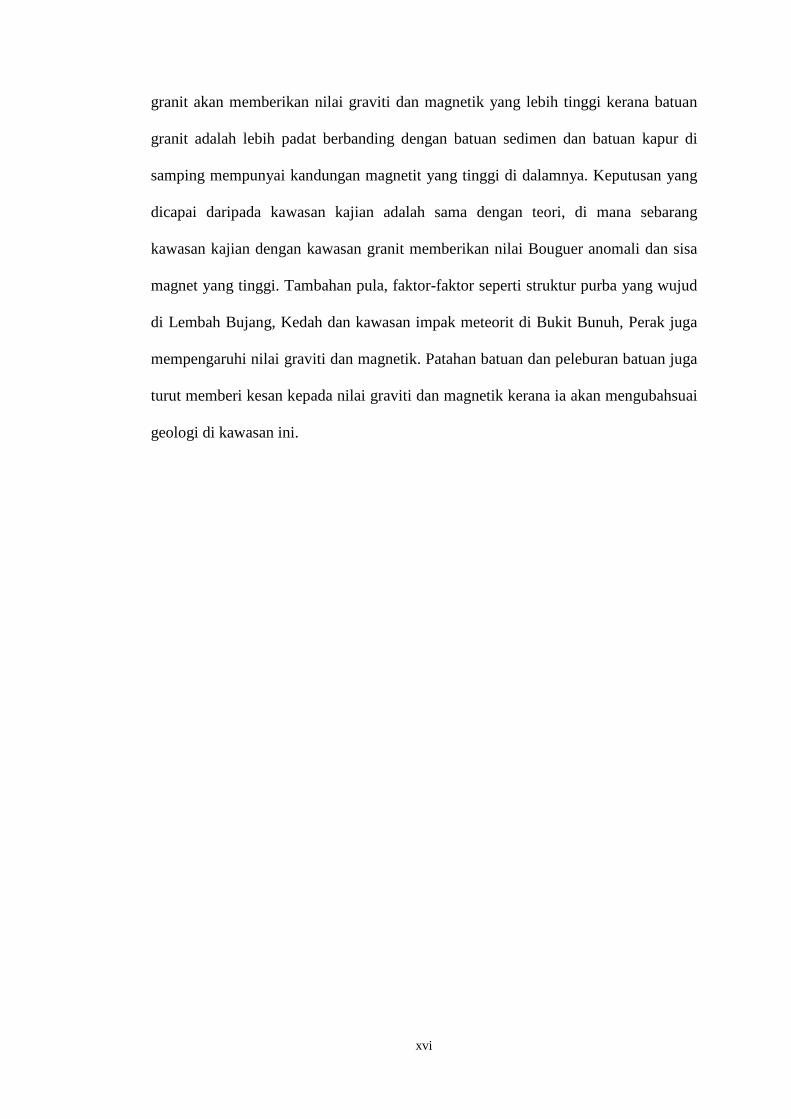
xvi
granit akan memberikan nilai graviti dan magnetik yang lebih tinggi kerana batuan
granit adalah lebih padat berbanding dengan batuan sedimen dan batuan kapur di
samping mempunyai kandungan magnetit yang tinggi di dalamnya. Keputusan yang
dicapai daripada kawasan kajian adalah sama dengan teori, di mana sebarang
kawasan kajian dengan kawasan granit memberikan nilai Bouguer anomali dan sisa
magnet yang tinggi. Tambahan pula, faktor-faktor seperti struktur purba yang wujud
di Lembah Bujang, Kedah dan kawasan impak meteorit di Bukit Bunuh, Perak juga
mempengaruhi nilai graviti dan magnetik. Patahan batuan dan peleburan batuan juga
turut memberi kesan kepada nilai graviti dan magnetik kerana ia akan mengubahsuai
geologi di kawasan ini.
xvii
GRAVITY AND MAGNETIC DATA REDUCTION SOFTWARE
(GraMag2DCon) FOR SITES CHARACTERIZATION
ABSTRACT
Present potential field methods software are focuses more on data
interpretation and analysis which resulted in the lack of data processing software for
potential field methods. This caused processing gravity and magnetic methods
become a tedious task as one will opted either to manually process the data or used
the complicated software which focuses more on data modeling and filtering. By
developing new software named GraMag2DCon which include the combination of
both gravity and magnetic data processing, data processing for potential field
methods will be much easier. GraMag2DCon software includes importing and
exporting the data, as well as able to edit any data during data processing. This
software also able to alert the user if any error or mistakes occur during data
processing which can save a lot of time. As the objectives of the study is to identify
and characterized gravity and magnetic values of different geological settings, data
acquisition of both gravity and magnetic methods are done in granitic area
(Universiti Sains Malaysia, Pulau Pinang), sedimentary area (Kaki Bukit, Perlis),
limestone area (Batu Caves, Kuala Lumpur), archaeological sites (Lembah Bujang,
Kedah) and meteorite impact region (Bukit Bunuh, Perak). Using GraMag2DCon
software, all of the data collected were processed so that gravity and magnetic values
for different types of geological area can be identified and characterized.
Theoretically, granitic area will give higher values of both gravity and magnetic
values as granitic rocks is much denser compare to sedimentary and limestone rock
and has high magnetite contents in it. The results achieved from the study areas are

xviii
similar to the theory, where any study area with granitic area gives high values of
Bouguer anomaly and magnetic residual. Furthermore, factors such as ancient
structures exist in Lembah Bujang, Kedah and meteorite impact region in Bukit
Bunuh, Perak also influenced the gravity and magnetic values. Rock fracturing and
rock melting also affect the gravity and magnetic values as it will modify the
geology of the area.
1
CHAPTER 1
INTRODUCTION
1.0 Background
Geophysical methods provide a relatively rapid and cost-effective in
acquiring information about the subsurface over a substantial area. Geophysics is the
application of physics principles to study the Earth subsurface properties. The aim of
pure geophysics is to deduce physical properties of the Earth and its internal
constitution from physical phenomena associated with it such as gravity force and
geomagnetic field (Burger et al., 2006). Geophysics essentially is the measurement
of contrasts in physical properties of materials beneath the Earth’s surface and
attempt to deduce the nature and distribution of materials responsible for these
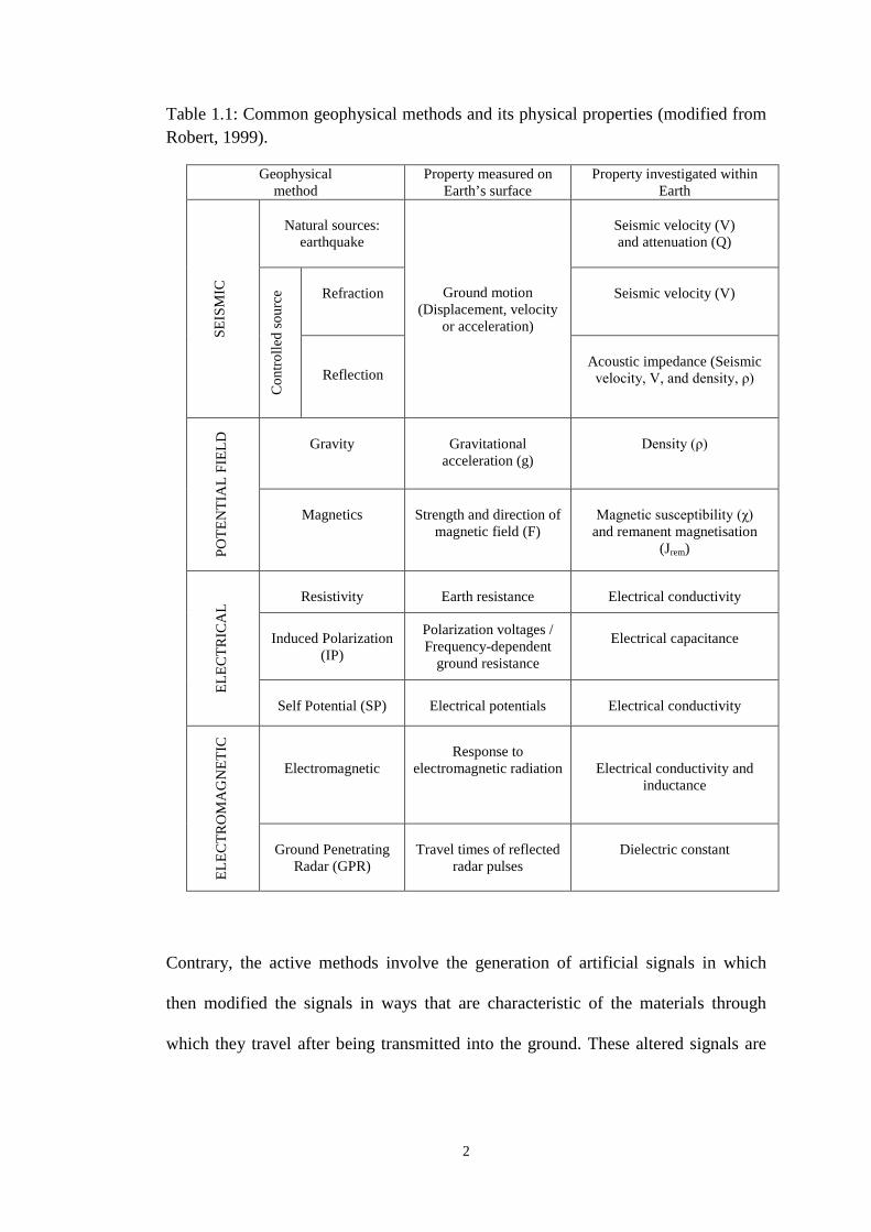
observations. Four types of common geophysical methods and its physical properties
are lists in the Table 1.1.
It is proven that geophysical methods are able to detect and delineate local
features of potential interest which could not be discovered by any drilling method
although sometimes it is prone to major ambiguities or uncertainties of
interpretations. The uncertainties can be overcome by having a good geological
background and full knowledge of the area. This will lead to correct interpretation
and reduced the uncertainties.
Geophysical methods are classified into two types, passive and active
methods. Those methods that detect variations within the natural fields associated
with the Earth such as the gravitational and magnetic fields are passive methods.
2
Table 1.1: Common geophysical methods and its physical properties (modified from Robert, 1999).
Geophysical method
Property measured on Earth’s surface
Property investigated within Earth
SE
ISM
IC
Natural sources:
earthquake
Ground motion (Displacement, velocity
or acceleration)
Seismic velocity (V) and attenuation (Q)
C
ontro
lled
sour
ce
Refraction
Seismic velocity (V)
Reflection
Acoustic impedance (Seismic
velocity, V, and density, ρ)
PO
TEN
TIA
L FI
ELD
Gravity
Gravitational
acceleration (g)
Density (ρ)
Magnetics
Strength and direction of
magnetic field (F)
Magnetic susceptibility (χ)
and remanent magnetisation (Jrem)
EL
ECTR
ICA
L
Resistivity
Earth resistance
Electrical conductivity
Induced Polarization
(IP)
Polarization voltages / Frequency-dependent
ground resistance
Electrical capacitance
Self Potential (SP)
Electrical potentials
Electrical conductivity
EL
ECTR
OM
AG
NET
IC
Electromagnetic
Response to
electromagnetic radiation
Electrical conductivity and inductance
Ground Penetrating
Radar (GPR)
Travel times of reflected
radar pulses
Dielectric constant
Contrary, the active methods involve the generation of artificial signals in which
then modified the signals in ways that are characteristic of the materials through
which they travel after being transmitted into the ground. These altered signals are
3
then measured by appropriate instruments where the output displayed and interpreted
(Edet, 2010). Geophysical methods are one of the fastest, most effective, least costly
and an indirect method to perform shallow subsurface study for maintaining
infrastructure and geo-environment (Muztaza, 2013).
Seismic method commonly applies to determine rock velocities and quality,
stratigraphy, general geologic structure, overburden thickness and bedrock depth. It
manipulates energy sources created by shot, hammer, weight drop or some other
comparable sources by putting impulsive energy into the ground (Burger et al.,
2006). Generally, 2-D resistivity method measures an apparent resistivity of
subsurface including soil type effects, bedrock fractures, groundwater and
contaminants. Ground Penetrating Radar (GPR) provides a cross-sectional
measurement of the shallow subsurface and used to pinpoint the location of buried
objects as well as mapping stratigraphy. It also allows registration of such fine
archaeological objects that are hard to see by naked eye and can be missed during
archaeological excavation (Conyers, 2004).
Gravity and magnetic methods also known as potential field method are very
useful and popular in geological case studies. By manipulating density variation of
subsurface and magnetic susceptibilities, the methods lead to variations in
gravitational acceleration at surface instrument stations and produce measurable
differences of magnetic field at observation sites (Burger et al., 2006). The methods
provide a low cost way to screen large areas as well as construct important
alternative models to delineate subsurface structures and reach a better understanding
of geology (Rivas, 2009). Mapping the Earth’s subsurface using potential field
method is common and widely use around the world including in Malaysia. Fault
4
and fractures, basin, bedrock topography, geological structure and boundaries as well
as meteorite impact crater can be map by utilizing gravity and magnetic methods.
The gravity method depends on a high-density contrast between the geologic
bodies of interest and that of the surrounding sediment (Jacques et al., 2003).
Natural variations in subsurface density include lateral changes of soil or rock
density, buried channels, large fractures, faults and cavities. A good processing
method can provide a good estimate of depth, size and nature of anomaly. Irregular
topography will produce artefacts in the data, unless it is accounted for in the
processing. As the microgravimeter is very sensitive, interference can be produce by
external factors such as local sources of vibrations, wind, storms, atmospheric
pressure, station elevation and distance earthquakes (Seigel, 1995). Thus, data
assessment is very important to eliminate such artefacts. Gravity method applications
include fault mapping, groundwater inventories, basin studies and mineral
exploration.
Magnetic data can be analyzed in a number of ways, with enhanced
techniques and imaging, hence making it an increasingly valuable tool. The basic
geophysical concept behind this is that different rock types having different magnetic
responses. The magnetic method does not give exact depth determination (Grauch
and Lindrith, 2005). It can be apply to both, deep and shallow structures which
measurements can be obtained for both local and regional studies (Burger et al.,
2006). This method is typically applied to locate abandoned steel well casings,
buried tanks and pipes, map basement faults and basic igneous intrusive, investigate
archaeological sites and map old waste sites and landfill boundaries (Mariita, 2007).
5
Although geophysical methods are useful and provide valuable information
about the subsurface, it is important to recognize their limitations (Burger et al.,
2006). The lack of sufficient contrast in physical properties is common as one of the
limitation and a good instrument can determine the effects. The presence of nearby
bodies of great contrasts creates effects that mask those created by the targeted
object frequently cause problems. The second limitation is the non uniqueness of the
interpretation. For example in gravity method, ambiguity tends to happen when it is
often difficult to differentiate the effect of a small body near the surface from that of
a larger body at very deep. The third limitation is resolution. All methods are
afflicted with this restriction. The last limitation is noise. All geophysical data
contain some undesired signal (or noise) to a greater or lesser extent.
Each of geophysical method has its own advantages and disadvantages. The
limitations can be overcome by integrating two or more methods for each
study/research. A careful survey planning, desk study, a good geological
background and knowledge of the area are the key for good data acquisition and
essential for good interpretation.
Gravity and magnetic methods need to be corrected for all of its raw data
before interpretation step. This step is called processing step and involves a lot of
corrections. Most of the software existed in the market are focuses more on
interpretation step which involves modeling and more on quantitative interpretations.
Most of these software are also very expensive and complicated to use.
6
1.1 Problem statements
The potential field methods markets are flooded with software that focuses
more on interpretations rather than processing step. The lack of data processing
software triggered the start of this research. With little choices to choose from the
present software, it is best to develop new processing software that are not
complicated and focuses on processing step. Data processing plays a very crucial
part in geophysics methods especially in potential field methods. It has many
corrections to be made depending on the objectives of the survey. The problem lies
as different people processed the same data with the same objective but getting
different results. It can be consider as systematic error. Having to do all the data
correction manually using Microsoft Excel with all hundreds or thousands of data,
mistakes are bound to happen. To go through one by one of those hundreds of data to
find the mistake is one tedious task and wasting time.
To overcome this problem, it is useful to develop the new processing
software. Other additional corrections can be done depending on the objective and
types of survey (ground, air or marine) with this basic processing. The new software
will be compute in such a way that the final results can be obtain by input or
exporting raw data, elevation and coordinates (latitude and longitude) of the survey
stations. By computing this new software, it is hoped that it can be beneficiary for
basic magnetic and gravity data processing.
7
1.2 Objectives
The objectives of the research are:
i. To develop a new gravity and magnetic data reduction processing
software.
ii. To identify gravity and magnetic values of different bedrock geological
settings in Peninsular Malaysia.
iii. To characterize the gravity and magnetic data for different geological
settings.
1.3 Significance and novelties
The study mainly aims to produce data reduction processing software for
potential field methods since many data corrections/reductions need to be done.
Using the newly developed software, systematic error which usually happened
during data reduction processing can be minimized. Unlike any other potential
software processing, this new software is only for ground survey and is only for data
reduction where else other potential field software mainly focus on modelling and
filtering. The software will indicate the error or mistake if it encounters any
mistakes. Furthermore, the software is time effective, user friendly and not
complicated like other existed software. One can operate it without reading the
software manual. Thus, by using the software in different geological settings of the
study areas, value range for bedrock from different geological settings can be
identified and characterized.
8
1.4 Thesis layout
Chapter 1 introduce background of geophysical methods which focuses more
on gravity and magnetic methods, stating problem statements and ways to overcome
the problems. Objectives and novelties of the research are also pointed out in this
chapter.
Chapter 2 discusses on theory of potential field methods (gravity and
magnetic method), the similarities and the differences between the two methods as
well as some previous study of both methods and other geophysical methods with
application in geological cases, archaeology and meteorite impact. Some previous
studies on other existed potential field software are also included.
Chapter 3 focuses on methodology where it discusses on the research
methodology of potential field method, geological settings of study areas besides
data acquisition execution. The research involves developing processing software for
potential field methods.
Chapter 4 elaborate more on the software development. From how it is
developed to step by step in using the new software are explained in this chapter.
Chapter 5 discusses on the potential field methods applications in different
geological settings. The acquired gravity and magnetic data were processed using the
newly developed processing software. Results of the research will be presented in
this chapter as well as more discussions on the results and the advantages of the
newly developed software.
9
Chapter 6 as the final chapter in the thesis concludes the findings done
including some recommendations for future findings.
10
CHAPTER 2
LITERATURE REVIEW
2.0 Introduction
Potential field methods measure natural fields of the Earth which are
gravitational and magnetic fields. Both methods utilized natural occurring fields and
provide information on Earth properties to significantly greater depth. Gravity and
magnetic methods detect only lateral contrasts in density or magnetization. Density
and magnetization change significantly from one soil or rock types to another.
Knowledge of the distribution of any of these properties within the ground would
presumably convey information of great potential value about subsurface geology,
even if the soil/rocks themselves could not be otherwise identified (Grant and West,
1965).
Both gravity and magnetic methods have been employed in diversified ways
for mineral exploration, oil and gas exploration, environmental and engineering,
education and research, earthquake prediction, geotechnical and mining related
airborne geophysical surveys. Gravity data can be used to model the shape of a basin
containing young sedimentary rocks compared to higher density basement rocks.
On the other hand, magnetic data can provide complementary information if
there is a magnetic contrast between the sedimentary rocks and the basement. To
understand the movement of subsurface water, mapping of sediment/basement is
important. By mapping offsets of both gravity and magnetic source bodies faults can
11
be traced (Ken et al., 2001). Dykes, faults and lava flows, finding abandoned wells
and buried drum, and locating and mapping waste dumps are amongst the common
causes of magnetic anomalies. The survey can be carried out on land, marine and in
the air. The methods were widely used as both methods are relatively cheap, non-
invasive and non-destructive towards the environment. Potential fields are those in
which the strength and direction of the field depend on the position within the field;
the strength of a potential field decreases with distance from the source (Robert,
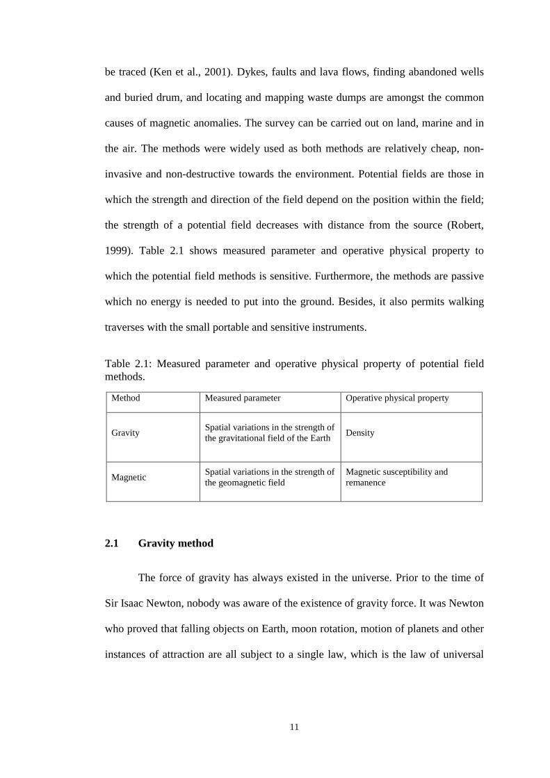
1999). Table 2.1 shows measured parameter and operative physical property to
which the potential field methods is sensitive. Furthermore, the methods are passive
which no energy is needed to put into the ground. Besides, it also permits walking
traverses with the small portable and sensitive instruments.
Table 2.1: Measured parameter and operative physical property of potential field methods.
Method Measured parameter Operative physical property
Gravity Spatial variations in the strength of the gravitational field of the Earth Density
Magnetic Spatial variations in the strength of the geomagnetic field
Magnetic susceptibility and remanence
2.1 Gravity method
The force of gravity has always existed in the universe. Prior to the time of
Sir Isaac Newton, nobody was aware of the existence of gravity force. It was Newton
who proved that falling objects on Earth, moon rotation, motion of planets and other
instances of attraction are all subject to a single law, which is the law of universal
12
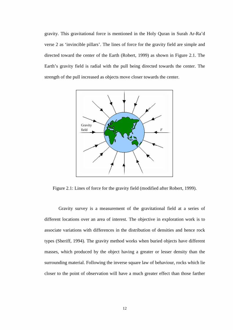
gravity. This gravitational force is mentioned in the Holy Quran in Surah Ar-Ra’d
verse 2 as ‘invincible pillars’. The lines of force for the gravity field are simple and
directed toward the center of the Earth (Robert, 1999) as shown in Figure 2.1. The
Earth’s gravity field is radial with the pull being directed towards the center. The
strength of the pull increased as objects move closer towards the center.
Figure 2.1: Lines of force for the gravity field (modified after Robert, 1999).
Gravity survey is a measurement of the gravitational field at a series of
different locations over an area of interest. The objective in exploration work is to
associate variations with differences in the distribution of densities and hence rock
types (Sheriff, 1994). The gravity method works when buried objects have different
masses, which produced by the object having a greater or lesser density than the
surrounding material. Following the inverse square law of behaviour, rocks which lie
closer to the point of observation will have a much greater effect than those farther
Gravity field F
13
away even though all materials in the Earth influence gravity (Grant and West,
1965).
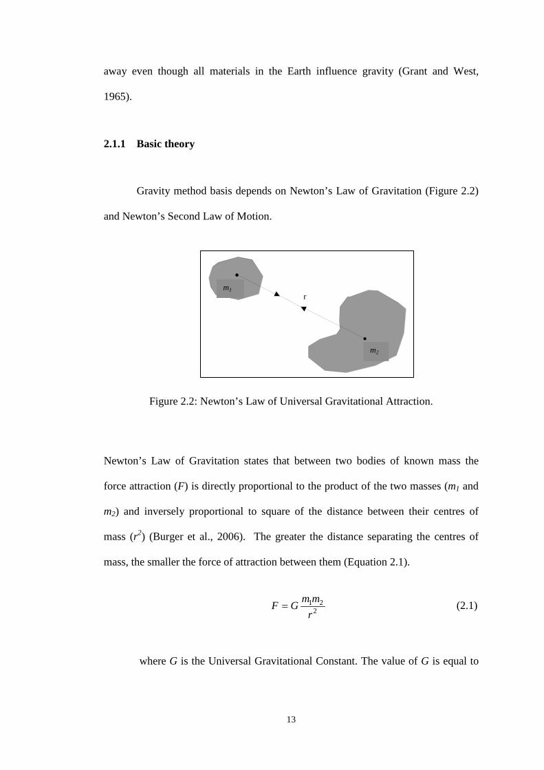
2.1.1 Basic theory
Gravity method basis depends on Newton’s Law of Gravitation (Figure 2.2)
and Newton’s Second Law of Motion.
M1
M2
r
F =GM1M2
r 2
Figure 2.2: Newton’s Law of Universal Gravitational Attraction.
Newton’s Law of Gravitation states that between two bodies of known mass the
force attraction (F) is directly proportional to the product of the two masses (m1 and
m2) and inversely proportional to square of the distance between their centres of
mass (r2) (Burger et al., 2006). The greater the distance separating the centres of
mass, the smaller the force of attraction between them (Equation 2.1).
221
rmmGF = (2.1)
where G is the Universal Gravitational Constant. The value of G is equal to
r
m2
m1
14
6.67× 10⁻¹¹ Nm2/kg2 in SI units. Newton’s Second Law of Motion (Robert, 1999)
shows that the force (F) exerted on the object with mass m1 by the body with mass
m2 (Equation 2.2),
amF 1= (2.2)
where a is acceleration of object with mass m1 due to the gravitational
attraction of the object with mass m2 (m/s2).
The combination of Equation 2.1 and 2.2 produced Equation 2.3.
221
11
1
r
mGm
mmFa ==
22
rGma = (2.3)
If the acceleration (a) is in a vertical direction, then it is due to gravity (g)
which gives a=g then it can be write as;
2RGMg = (2.4)
where M is mass of the Earth (M = m2) and R is distance from the observation
point to Earth’s center of mass (R = r).
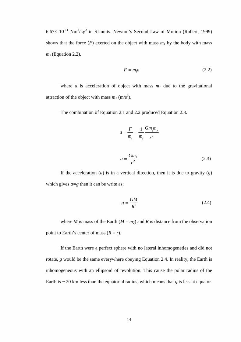
If the Earth were a perfect sphere with no lateral inhomogeneties and did not
rotate, g would be the same everywhere obeying Equation 2.4. In reality, the Earth is
inhomogeneous with an ellipsoid of revolution. This cause the polar radius of the
Earth is ~ 20 km less than the equatorial radius, which means that g is less at equator
15
than pole. At the equator, the value of gravitational acceleration on Earth’s surface
varies from 9.78 m/s2 to about 9.83 m/s2 at the poles (Figure 2.3).
Figure 2.3: Three main factors responsible for the difference in gravitational acceleration at the equator compared to the poles (modified after Robert, 1999).
The smaller acceleration at an equator, compared to the poles, is because of
the combination of three factors (Robert, 1999). The first factor is due to outward
acceleration caused by rotation of the Earth, there is less inward acceleration. The
rotation is greatest at the equator but reduces to zero at the poles. Second factor is
less acceleration at the equator because of the Earth’s outward bulging, thereby
increasing the radius (R) to the center of mass. Third factor is the added mass of the
bulge creates more acceleration. Notice that the first two factors lessen the
acceleration at the equator, while the third increases it. Gravitational acceleration
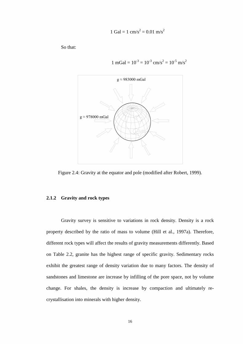
(gravity) is commonly expressed in miligals (mGal). Gravity increases from about
978 000 mGal at the equator, to about 983 000 mGal at the poles and varies by about
5000 mGal from equator to pole (Figure 2.4).
g ≈ 9.78 ms-2
g ≈ 9.83 ms-2
Increased Radius -∆g
Earth’s Rotation -∆g
Excess Mass
+∆g
R (equator)
R (p
ole)
16
1 Gal = 1 cm/s2 = 0.01 m/s2
So that:
1 mGal = 10-3 = 10-3 cm/s2 = 10-5 m/s2
Figure 2.4: Gravity at the equator and pole (modified after Robert, 1999).
2.1.2 Gravity and rock types
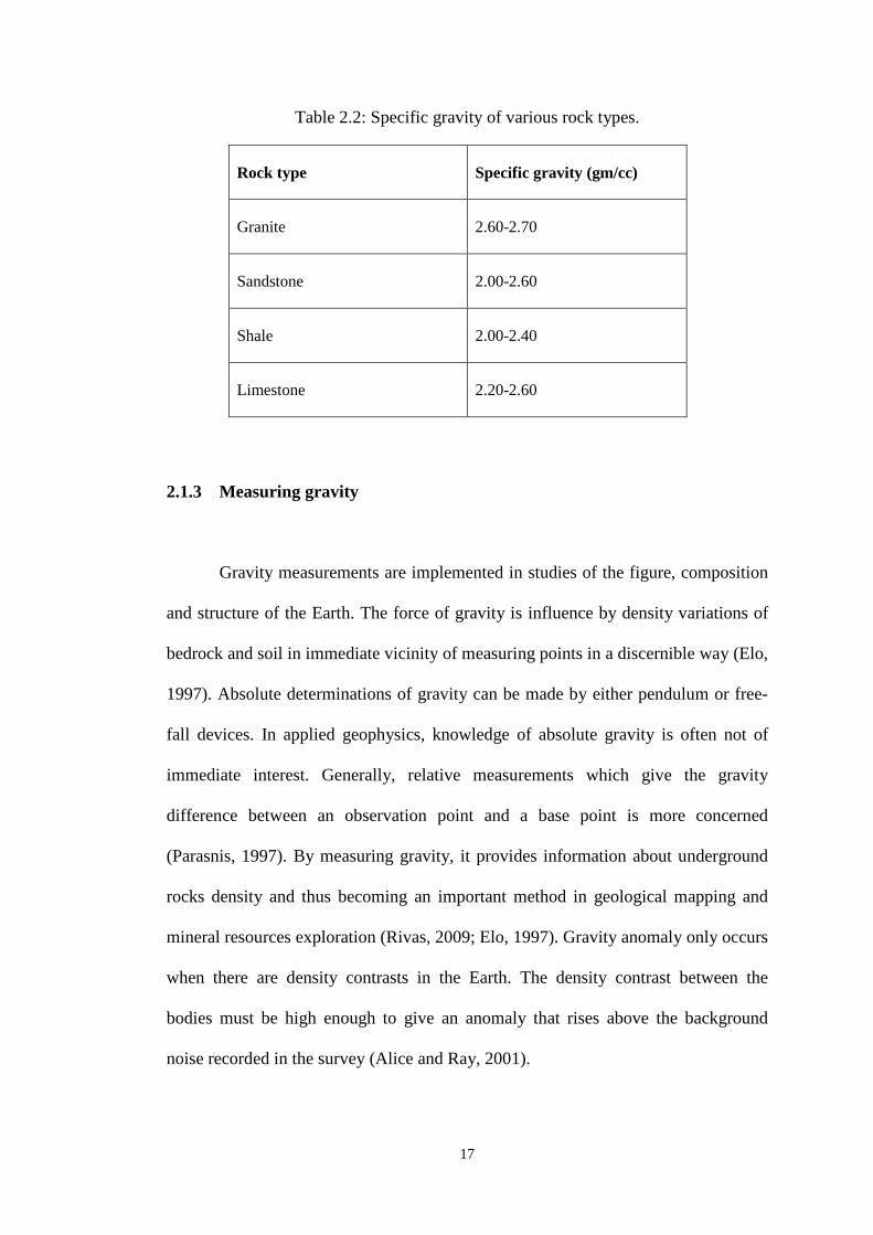
Gravity survey is sensitive to variations in rock density. Density is a rock
property described by the ratio of mass to volume (Hill et al., 1997a). Therefore,
different rock types will affect the results of gravity measurements differently. Based
on Table 2.2, granite has the highest range of specific gravity. Sedimentary rocks
exhibit the greatest range of density variation due to many factors. The density of
sandstones and limestone are increase by infilling of the pore space, not by volume
change. For shales, the density is increase by compaction and ultimately re-
crystallisation into minerals with higher density.
g ≈ 983000 mGal
g ≈ 978000 mGal
17
Table 2.2: Specific gravity of various rock types.
Rock type Specific gravity (gm/cc)
Granite 2.60-2.70
Sandstone 2.00-2.60
Shale 2.00-2.40
Limestone 2.20-2.60
2.1.3 Measuring gravity
Gravity measurements are implemented in studies of the figure, composition
and structure of the Earth. The force of gravity is influence by density variations of
bedrock and soil in immediate vicinity of measuring points in a discernible way (Elo,
1997). Absolute determinations of gravity can be made by either pendulum or free-
fall devices. In applied geophysics, knowledge of absolute gravity is often not of
immediate interest. Generally, relative measurements which give the gravity
difference between an observation point and a base point is more concerned
(Parasnis, 1997). By measuring gravity, it provides information about underground
rocks density and thus becoming an important method in geological mapping and
mineral resources exploration (Rivas, 2009; Elo, 1997). Gravity anomaly only occurs
when there are density contrasts in the Earth. The density contrast between the
bodies must be high enough to give an anomaly that rises above the background
noise recorded in the survey (Alice and Ray, 2001).
18
To determine acceleration due to gravity at various sites around the world,
instruments are designed and it is called gravity meters, also known as gravimeters.
Neither pendulum nor free-fall devices are suitable for field survey as it is not as
convenient as gravimeters and both of it measure absolute gravity. The gravimeters
are sensitive to 0.01 mGal ≈ 10-8 of the Earth’s total value. Instruments are designed
to measure gravity directly perform absolute measurements (Burger et al., 2006).
The field gravity survey conducted using relative gravimeters because it would be
impossible to get the accuracy required in absolute gravity measurements quickly
with any device. The gravimeter measures relative changes in between two locations
(Rivas, 2009).
Gravity prospecting can be conducted over land (ground), water (marine) and
air (airborne) using different techniques and equipment. Ground survey conducted
by walking traverses or using vehicle while marine survey used the meter onboard
ship and an aircraft is used for airborne survey. The airborne survey is always used
when confronting an inaccessible terrain and large survey area. The small portable
instrument makes gravity method can quickly cover large areas (Rivas, 2009).
2.1.4 Gravity reduction
In reality, the Earth is slightly irregular oblate ellipsoid which means that the
gravity field at its surface is stronger at the poles than the equator. The density
distribution is also uneven, particularly in the rigid crust, which causes gravity to
vary from the expected value as the measurement position changes. These variations
are expressed as gravity anomalies. By mapping the gravity anomalies, it gives an
19
insight structure of the Earth (Alice and Ray, 2001). Therefore, it is essential to
identify the reasons that gravity varies so it can be corrected while using gravity
method in exploring the subsurface (Burger et al., 2006). Gravity observations can
be used to interpret changes in mass below different regions of the Earth (Robert,
1999). The observed gravity readings obtained from the gravity survey reflect the
gravitational field due to all masses in the Earth and the effect of the Earth’s rotation.
To interpret gravity data, one must remove all known gravitational effects that are
not related to the subsurface density changes (Mickus, 2003). These include
latitudinal variations, elevation changes, topographic changes, building effects, the
Earth’s shape and rotation, and Earth tides (LaFehr, 1991). It is necessary to correct
for all of the factors that are not due to density contrasts in the subsurface
(Christopher, 2001). Raw gravity data were corrected for drift, height, free-air,
Bouguer, absolute gravity, terrain, theoretical gravity correction and finally obtaining
Bouguer anomaly value for mapping and interpretation.
2.1.4.1 Drift and tidal effect
If a gravimeter is placed in one position and readings are taken every hour or
so, the values obtained would vary. This variation is due to two causes. One is
instrument drift, which is caused by small changes in the physical constants of
gravimeter components (Burger et al., 2006). Due to elastic creep in the springs, the
readings of gravimeters drift more or less with time (Parasnis, 1997). This
instrument drift affects cannot be ignored due to an extreme sensitivity of
gravimeters (Burger et al., 2006). In order to correct for it, the measurements at a set
of stations are repeated after 1 to 2 hour and the differences obtained are plotted
20
against the time between two readings at a station (Parasnis, 1997). This reading
sequence is referred to as looping. The other cause is due to tidal effects that are
governed by the positions of the Sun and the Moon relative of the Earth. Observed
gravity readings at a fixed location will change with time due to the periodic motion
of the Sun and the Moon (Christopher, 2001). Tidal variations produce an effect on
gravimeter mass that varies by ± 0.15 mGal from a mean value and can have a rate
of change as high as 0.05 mGal/ hour. Because there are substantial values relative to
the 0.01 precision of most gravimeters, a correction clearly is called for. Tidal effects
can be predicted accurately, so it is relatively straightforward to a computer program
to produce values for any location at any time (Burger et al., 2006). For Scintrex
(gravimeter), software is supplied to automatically remove the Earth tide effect.
2.1.4.2 Latitude effect
The value of gravity increases with the geographical latitude (Parasnis,
1997). Due to the Earth’s rotation, the Earth is not spherical but is flattened at the
poles. This means that the length of the Earth’s radius is greater at the equator than at
the poles. This distance factor causes the g value to increase from equator to pole by
6.6 Gals because of the surface is closer to the center of the Earth at the poles
(Burger et al., 2006).
2.1.4.3 Free-air correction
Gravity observed at a specific location on Earth’s surface can be viewed as a
function of three main components which are observation point latitude, station
21
elevation and mass distribution in the subsurface. Free-air correction accounts for
second effect, which is the local change in gravity due to elevation difference
between station and sea level (Robert, 1999; Hill et al., 1997a). In practice the value
of 0.3086 mGal/m is the only value used after deriving from Equation (2.4) and
assumed that the Earth is spherical and non-rotating (Equation 2.5). Note that this
correction considers only elevation differences relative to a datum and does not take
into account that the mass between the observations point and datum, as if the
stations were suspended in free air, not sitting on land. This is the reason the
correction is termed as free-air correction. Normally the datum used for gravity
surveys is sea level and gravity decreases 0.3086 mGal for every meter above sea
level (Burger et al., 2006).
2RGMg =
FACrg
rGm
drdg
=−=−=22
2
m
mGalrgFAC 3086.02== (2.5)
where FAC is free-air correction.
2.1.4.4 Bouguer correction
Even after elevation correction, gravity can vary from station to station
because of differences in mass between the observation points and sea-level datum
22
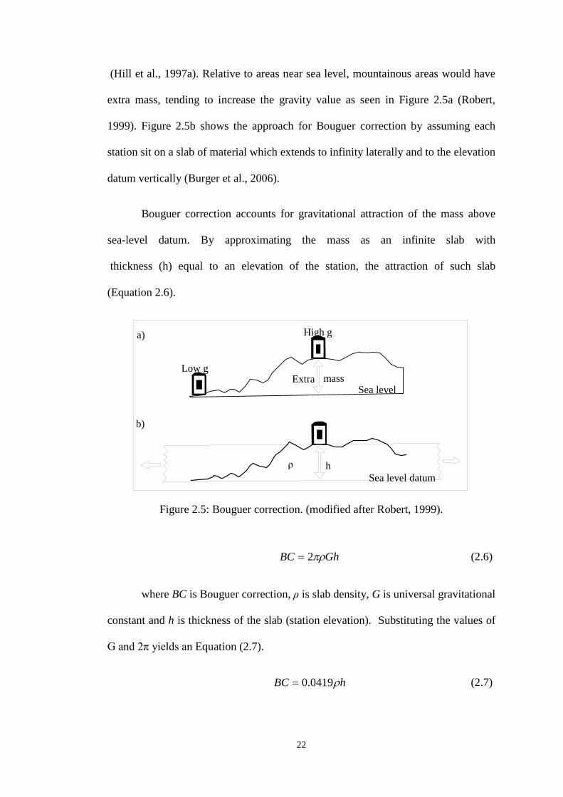
(Hill et al., 1997a). Relative to areas near sea level, mountainous areas would have
extra mass, tending to increase the gravity value as seen in Figure 2.5a (Robert,
1999). Figure 2.5b shows the approach for Bouguer correction by assuming each
station sit on a slab of material which extends to infinity laterally and to the elevation
datum vertically (Burger et al., 2006).
Bouguer correction accounts for gravitational attraction of the mass above
sea-level datum. By approximating the mass as an infinite slab with
thickness (h) equal to an elevation of the station, the attraction of such slab
(Equation 2.6).
Figure 2.5: Bouguer correction. (modified after Robert, 1999).
GhBC πρ2= (2.6)
where BC is Bouguer correction, ρ is slab density, G is universal gravitational
constant and h is thickness of the slab (station elevation). Substituting the values of
G and 2π yields an Equation (2.7).
hBC ρ0419.0= (2.7)
a)
b)
Low g
High g
Extra mass Sea level
Sea level datum ρ h
23
where BC is in mGal (10-5 m/s2); ρ in g/cm3 (103 kg/m3); h in m.
Using the Nettleton’s approach, gravity data were to reduce by using 2.67
g/cm density. This is because this value caused the least influence of relief features
which is a few ten meters on the resulting gravity data (Rybakov et al., 2010).
2.1.4.5 Terrain correction
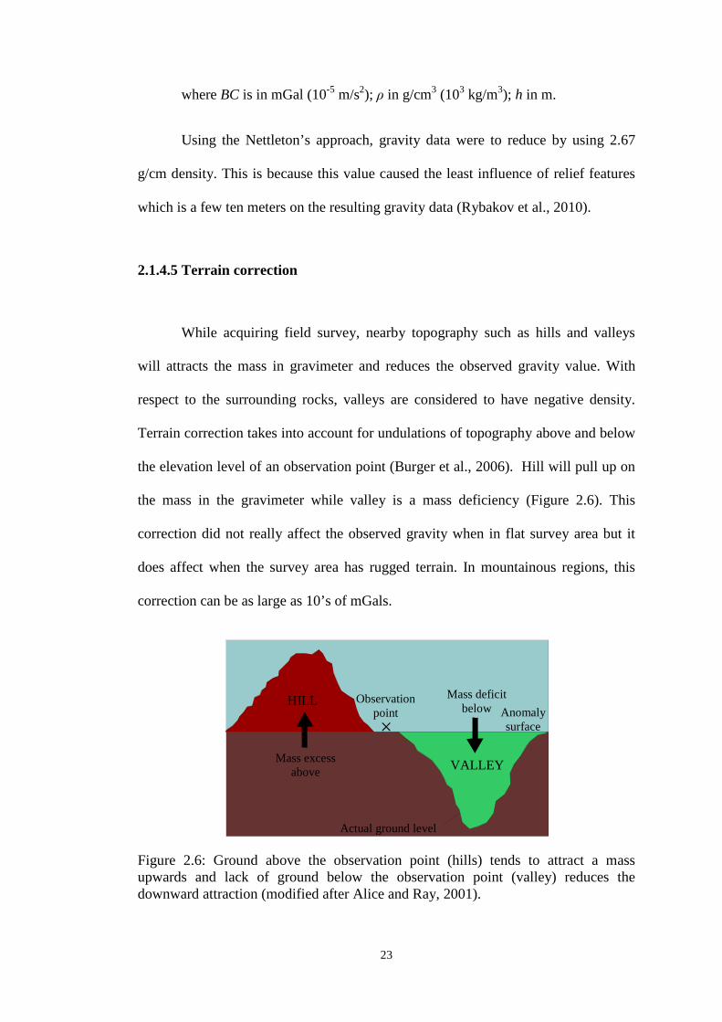
While acquiring field survey, nearby topography such as hills and valleys
will attracts the mass in gravimeter and reduces the observed gravity value. With
respect to the surrounding rocks, valleys are considered to have negative density.
Terrain correction takes into account for undulations of topography above and below
the elevation level of an observation point (Burger et al., 2006). Hill will pull up on
the mass in the gravimeter while valley is a mass deficiency (Figure 2.6). This
correction did not really affect the observed gravity when in flat survey area but it
does affect when the survey area has rugged terrain. In mountainous regions, this
correction can be as large as 10’s of mGals.
Figure 2.6: Ground above the observation point (hills) tends to attract a mass upwards and lack of ground below the observation point (valley) reduces the downward attraction (modified after Alice and Ray, 2001).
HILL
VALLEY
Observation point
Mass deficit below Anomaly
surface
Mass excess above
Actual ground level
24
2.2 Magnetic method
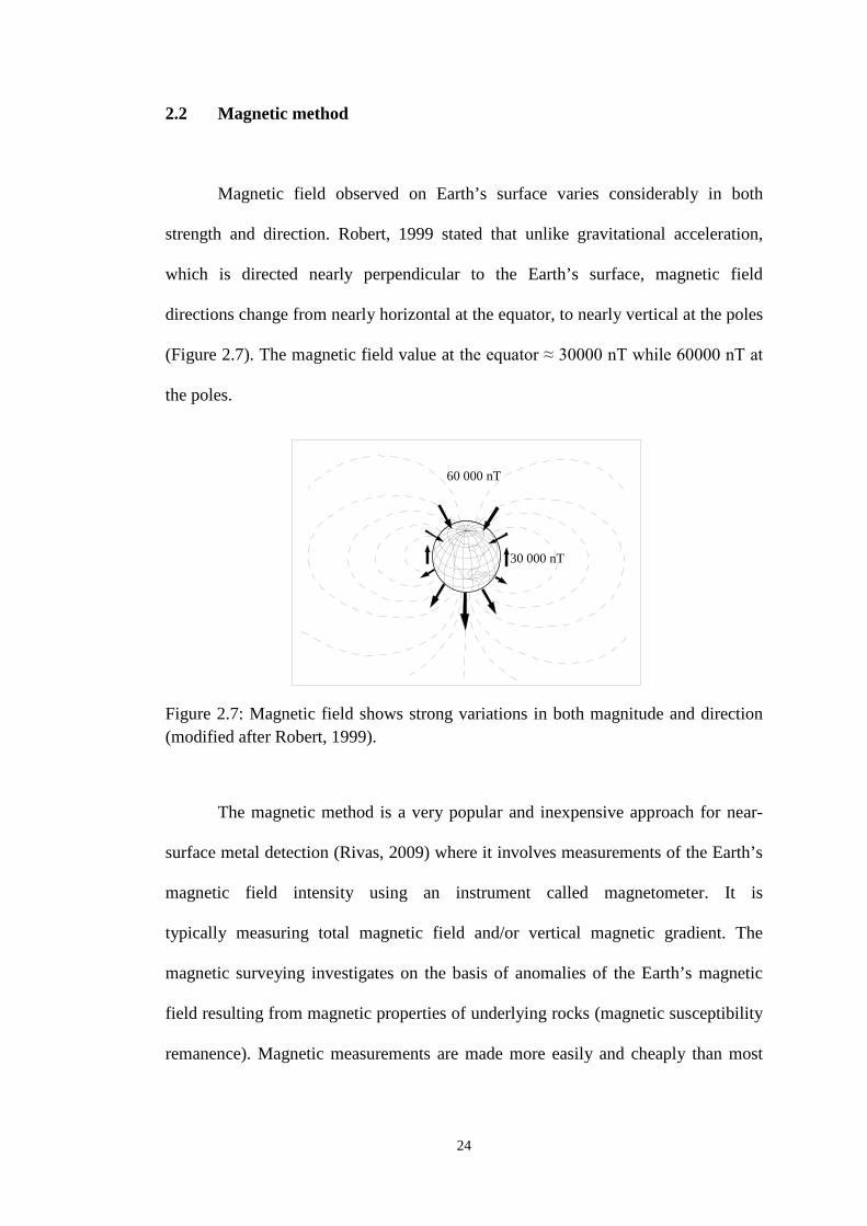
Magnetic field observed on Earth’s surface varies considerably in both
strength and direction. Robert, 1999 stated that unlike gravitational acceleration,
which is directed nearly perpendicular to the Earth’s surface, magnetic field
directions change from nearly horizontal at the equator, to nearly vertical at the poles
(Figure 2.7). The magnetic field value at the equator ≈ 30000 nT while 60000 nT at
the poles.
Figure 2.7: Magnetic field shows strong variations in both magnitude and direction (modified after Robert, 1999).
The magnetic method is a very popular and inexpensive approach for near-
surface metal detection (Rivas, 2009) where it involves measurements of the Earth’s
magnetic field intensity using an instrument called magnetometer. It is
typically measuring total magnetic field and/or vertical magnetic gradient. The
magnetic surveying investigates on the basis of anomalies of the Earth’s magnetic
field resulting from magnetic properties of underlying rocks (magnetic susceptibility
remanence). Magnetic measurements are made more easily and cheaply than most
30 000 nT
60 000 nT