Graph-Based Object Classification for Neuromorphic Vision Sensing

Yin Bi, Aaron Chadha, Alhabib Abbas, Eirina Bourtsoulatze and Yiannis Andreopoulos

Department of Electronic & Electrical Engineering

University College London, London, U.K.

{yin.bi.16, aaron.chadha.14, alhabib.abbas.13, e.bourtsoulatze, i.andreopoulos}@ucl.ac.uk

Abstract

Neuromorphic vision sensing (NVS) devices represent

visual information as sequences of asynchronous discrete

events (a.k.a., “spikes”) in response to changes in scene re-

flectance. Unlike conventional active pixel sensing (APS),

NVS allows for significantly higher event sampling rates at

substantially increased energy efficiency and robustness to

illumination changes. However, object classification with

NVS streams cannot leverage on state-of-the-art convolu-

tional neural networks (CNNs), since NVS does not pro-

duce frame representations. To circumvent this mismatch

between sensing and processing with CNNs, we propose

a compact graph representation for NVS. We couple this

with novel residual graph CNN architectures and show that,

when trained on spatio-temporal NVS data for object clas-

sification, such residual graph CNNs preserve the spatial

and temporal coherence of spike events, while requiring less

computation and memory. Finally, to address the absence

of large real-world NVS datasets for complex recognition

tasks, we present and make available a 100k dataset of NVS

recordings of the American sign language letters, acquired

with an iniLabs DAVIS240c device under real-world condi-

tions.

1. Introduction

Object classification finds numerous applications in vi-

sual surveillance, human-machine interfaces, image re-

trieval and visual content analysis systems. Following the

prevalence and advances of CMOS active pixel sensing

(APS), deep convolutional neural networks (CNNs) have

already achieved good performance in APS-based object

classification problems [28, 24]. However, APS-based sens-

ing is known to be cumbersome for machine learning sys-

tems because of limited frame rate, high redundancy be-

tween frames, blurriness due to slow shutter adjustment un-

der varying illumination, and high power requirements [18].

Inspired by the photoreceptor-bipolar-ganglion cell infor-

mation flow in low-level mammalian vision, researchers

Figure 1: Examples of objects captured by APS and neu-

romorphic vision sensors. Left: Conventional APS im-

age. Right: Events stream from NVS sensor (Red:ON,

Blue:OFF).

have devised cameras based on neuromorphic vision sens-

ing (NVS) [18, 51, 42]. NVS hardware outputs a stream

of asynchronous ON/OFF address events (a.k.a., “spikes”)

that indicate the changes in scene reflectance. An exam-

ple is shown in Fig 1, where the NVS-based spike events

correspond to a stream of coordinates and timestamps of re-

flectance events triggering ON or OFF in an asynchronous

manner. This new principle significantly reduces the mem-

ory usage, power consumption and redundant information

across time, while offering low latency and very high dy-

namic range.

However, it has been recognized that current NVS-

based object classification systems are inferior to APS-

based counterparts because of the limited amount of work

on NVS object classification and the lack of NVS data with

reliable annotations to train and test with [18, 42, 60]. In

this work, we improve on these two issues by firstly propos-

ing graph-based object classification method for NVS data.

Previous approaches have either artificially grouped events

into frame forms [65, 16, 13, 12] or derived complex fea-

ture descriptors [57, 15, 29], which do not always provide

for good representations for complex tasks like object clas-

sification. Such approaches dilute the advantages of com-

pactness and asynchronicity of NVS streams, and may be

sensitive to the noise and change of camera motion or view-

point orientation. To the best of our knowledge, this is the

1491

first attempt to represent neuromorphic spike events as a

graph, which allows us to use residual graph CNNs for end-

to-end task training and reduces the computation of the pro-

posed graph convolutional architecture to one-fifth of that

of ResNet50 [24], while outperforming or matching the re-

sults of the state-of-the-art.

With respect to benchmarks, most neuromorphic

datasets for object classification available to date are gen-

erated from emulators [40, 6, 23], or recorded from APS

datasets via recordings of playback in standard monitors

[53, 33, 25]. However, datasets acquired in this way can-

not capture scene reflectance changes as recorded by NVS

devices in real-world conditions. Therefore, creating real-

world NVS datasets is important for the advancement of

NVS-based computer vision. To this end, we create and

make available a dataset of NVS recordings of 24 letters

(A-Y, excluding J) from the American sign language. Our

dataset provides more than 100K samples, and to our best

knowledge, this is the largest labeled NVS dataset acquired

under realistic conditions.

We summarize our contributions as follows:

1. We propose a graph-based representation for neuro-

morphic spike events, allowing for fast end-to-end task

training and inference.

2. We introduce residual graph CNNs (RG-CNNs) for

NVS-based object classification. Our results show that

they require less computation and memory in compar-

ison to conventional CNNs, while achieving superior

results to the state-of-the-art in various datasets.

3. We source one of the largest and most challenging neu-

romorphic vision datasets, acquired under real-world

conditions, and make it available to the research com-

munity.

In Section 2 we review related work. Section 3 details

our method for NVS-based object classification and is fol-

lowed by the description of our proposed dataset in Section

4. Experimental evaluation is presented in Section 5 and

Section 6 concludes the paper.

2. Related Work

We first review previous work on NVS-based object clas-

sification, followed by a review of recent developments in

graph convolutional neural networks.

2.1. Neuromorphic Object Classification

Feature descriptors for object classification have been

widely used by the neuromorphic vision community. Some

of the most common descriptors are corner detectors and

line/edge extraction [14, 61, 39, 40]. While these efforts

were promising early attempts for NVS-based object clas-

sification, their performance does not scale well when con-

sidering complex datasets. Inspired by their frame-based

counterparts, optical flow methods have been proposed as

feature descriptors for NVS [15, 5, 3, 4, 10, 45]. For a

high-accuracy optical flow, these methods have very high

computational requirements, which diminishes their usabil-

ity in real-time applications. In addition, due to the inherent

discontinuity and irregular sampling of NVS data, deriving

compact optical flow representations with enough descrip-

tive power for accurate classification and tracking still re-

mains a challenge [15, 5, 10, 45]. Lagorce proposed event-

based spatio-temporal features called time-surfaces [29].

This is a time oriented approach to extract spatio-temporal

features that are dependent on the direction and speed of

motion of the objects. Inspired by time-surfaces, Sironi pro-

posed a higher-order representation for local memory time

surfaces that emphasizes the importance of using the infor-

mation carried by past events to obtain a robust representa-

tion [57]. A drawback of these methods is their sensitivity

to noise and their strong dependencies on the type of motion

of the objects in each scene.

Another avenue for NVS-based object classification is

via frame-based methods, i.e., converting the neuromorphic

events to into synchronous frames of spike events, on which

conventional computer vision techniques can be applied.

Zhu [65] introduced a four-channel image form with the

same resolution as the neuromorphic vision sensor: the first

two channels encode the number of positive and negative

events that have occurred at each pixel, while last two chan-

nels as the timestamp of the most recent positive and neg-

ative event. Inspired by the functioning of Spiking Neural

Networks (SNNs) to maintain memory of past events, leaky

frame integration has been used in recent work [16, 13, 12],

where the corresponding position of the frame is incre-

mented by a fixed amount when an event occurs at that

event address. Peng [48] proposed bag-of-events (BOE)

feature descriptors, which is a statistical learning method

that firstly divides the event streams into multiple segments

and then relies on joint probability distribution of the con-

secutive events to represent feature maps. However, these

methods do not offer the compact and asynchronous nature

of NVS, as the frame sizes that need to be processed are

substantially larger than those of the original NVS streams.

The final type of neuromorphic object classification is

event-based methods. The most commonly used architec-

ture is based on spiking neural networks (SNNs) [1, 19, 7,

30, 41]. While SNNs are theoretically capable of learn-

ing complex representations, they have still not achieved

the performance of gradient-based methods because of lack

of suitable training algorithms. Essentially, since the acti-

vation functions of spiking neurons are not differentiable,

SNNs are not able to leverage on popular training methods

492

Graph

Construction

Non-uniform

SamplingEvents Sampling

Graph

Convolution Nets

Label

Graph

G(0)G(1)cluster

Pooling Layer

***

Full

yC

onnec

ted

Conv (K=1) Batch Norm

Conv (K=5) Batch Norm

ReL

U

Graph Residual Block

So

ftM

ax

***

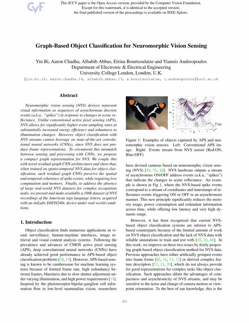
Figure 2: Framework of graph-based object classification for neuromorphic vision sensing.

such as backpropagation. To address this, researchers cur-

rently follow an intermediate step [44, 20, 49, 58]: a neu-

ral network is trained off-line using continuous/rate-based

neuronal models with state-of-the-art supervised training al-

gorithms and then the trained architecture is mapped to an

SNN. However, until now, despite their substantial imple-

mentation advantages at inference, the obtained solutions

are complex to train and have typically achieved lower per-

formance than gradient-based CNNs. Therefore, the pro-

posed graph-based CNN approach for NVS can be seen as

a way to bridge the compact, spike-based, asynchronous

nature of NVS with the power of well-established learning

methods for graph neural networks.

2.2. Graph CNNs

Generalizing neural networks to data with graph struc-

tures is an emerging topic in deep learning research. The

principle of constructing CNNs on graph generally follows

two streams: the spectral perspective [27, 32, 17, 62, 11,

52, 54] and the spatial perspective [21, 2, 8, 22, 36, 38].

Spectral convolution applies spectral filters on the spectral

components of signals on vertices transformed by a graph

Fourier transform, followed by spectral convolution. Def-

ferrard [17] provided efficient filtering algorithms by ap-

proximating spectral filters with Chebyshev polynomials

that only aggregate local K-neighborhoods. This approach

was further simplified by Kipf [27], who consider only the

one-neighborhood for single-filter operation. Levie [32]

proposed a filter based on the Caley transform as an al-

ternative for the Chebyshev approximation. As to spatial

convolution, convolution filters are applied directly on the

graph nodes and their neighbors. Several research groups

have independently dealt with this problem. Duvenaud [21]

proposed to share the same weights among all edges by

summing the signal over neighboring vertices followed by

a weight matrix multiplication, while Atwood [2] proposed

to share weights based on the number of hops between two

vertices. Finally, recent work [38, 22] makes use of the

pseudo-coordinates of nodes as input to determine how the

features are aggregated during locally aggregating feature

values in a local patch. Spectral convolution operations re-

quire an identical graph as input, as well as complex nu-

merical computations because they handle the whole graph

simultaneously. Therefore, to remain computationally effi-

cient, our work follows the spirit of spatial graph convolu-

tion approaches and extends them to NVS data for object

classification.

3. Methodology

Our goal is to represent the stream of spike events from

neuromorphic vision sensors as a graph and perform con-

volution on the graph for object classification. Our model

is visualized in Fig. 2: a non-uniform sampling strategy

is firstly used to obtain a small set of neuromorphic events

for computationally and memory-efficient processing; then

sampling events are constructed into a radius neighborhood

graph, which is processed by our proposed residual-graph

CNNs for object classification. The details will be described

in the following section.

3.1. Non­uniform Sampling & Graph Construction

Given a NVS sensor with spatial address resolution of

H × W , we express a volume of events produced by an

NVS camera as a tuple sequence:

{ei}N = {xi, yi, ti, pi}N (1)

493

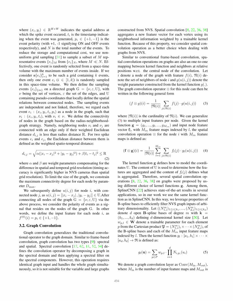
where (xi, yi) ∈ RH×W indicates the spatial address at

which the spike event occured, ti is the timestamp indicat-

ing when the event was generated, pi ∈ {+1,−1} is the

event polarity (with +1, -1 signifying ON and OFF events

respectively), and N is the total number of the events. To

reduce the storage and computational cost, we use non-

uniform grid sampling [31] to sample a subset of M rep-

resentative events {ei}M from {ei}N , where M ≪ N . Ef-

fectively, one event is randomly selected from a space-time

volume with the maximum number of events inside. If we

consider s{ei}ki=1 to be such a grid containing k events,

then only one event ei (i ∈ [1, k]) is randomly sampled

in this space-time volume. We then define the sampling

events {ei}{m} on a directed graph G = {ν, ε,U}, with

ν being the set of vertices, ε the set of the edges, and Ucontaining pseudo-coordinates that locally define the spatial

relations between connected nodes. The sampling events

are independent and not linked, therefore, we regard each

event ei : (xi, yi, ti, pi) as a node in the graph, such that

νi : (xi, yi, ti), with νi ∈ ν. We define the connectivity

of nodes in the graph based on the radius-neighborhood-

graph strategy. Namely, neighboring nodes νi and νj are

connected with an edge only if their weighted Euclidean

distance di,j is less than radius distance R. For two spike

events ei and ej , the Euclidean distance between them is

defined as the weighted spatio-temporal distance:

di,j =√

α(|xi − xj |2 + |yi − yj |2) + β|ti − tj |2 ≤ R

(2)

where α and β are weight parameters compensating for the

difference in spatial and temporal grid resolution (timing ac-

curacy is significantly higher in NVS cameras than spatial

grid resolution). To limit the size of the graph, we constrain

the maximum connectivity degree for each node by param-

eter Dmax.

We subsequently define u(i, j) for node i, with con-

nected node j, as u(i, j) = [|xi − xj | , |yi − yj |] ∈ U.After

connecting all nodes of the graph G = {ν, ε,U} via the

above process, we consider the polarity of events as a sig-

nal that resides on the nodes of the graph G. In other

words, we define the input feature for each node i, as

f (0)(i) = pi ∈ {+1,−1}.

3.2. Graph Convolution

Graph convolution generalizes the traditional convolu-

tional operator to the graph domain. Similar to frame-based

convolution, graph convolution has two types [9]: spectral

and spatial. Spectral convolution [17, 62, 11, 52, 54] de-

fines the convolution operator by decomposing a graph in

the spectral domain and then applying a spectral filter on

the spectral components. However, this operation requires

identical graph input and handles the whole graph simulta-

neously, so it is not suitable for the variable and large graphs

constructed from NVS. Spatial convolution [8, 22, 36, 38]

aggregates a new feature vector for each vertex using its

neighborhood information weighted by a trainable kernel

function. Because of this property, we consider spatial con-

volution operation as a better choice when dealing with

graphs from NVS.

Similar to conventional frame-based convolution, spa-

tial convolution operations on graphs are also an one-to-one

mapping between kernel function and neighbors at relative

positions w.r.t. the central node of the convolution. Let

i denote a node of the graph with feature f(i), N(i) de-

note the set of neighbors of node i and g(u(i, j)) denote the

weight parameter constructed from the kernel function g(.).The graph convolution operator ⊗ for this node can then be

written in the following general form

(f ⊗ g)(i) =1

|N(i)|

∑

j∈N(i)

f(j) · g(u(i, j)) (3)

where |N(i)| is the cardinality of N(i). We can generalize

(3) to multiple input features per node. Given the kernel

function g = (g1, ..., gl, ..., gMin) and input node feature

vector fl, with Min feature maps indexed by l, the spatial

convolution operation ⊗ for the node i with Min feature

maps is defined as:

(f ⊗ g)(i) =1

|N(i)|

Min∑

l=1

∑

j∈N(i)

fl(j) · gl(u(i, j)) (4)

The kernel function g defines how to model the coordi-

nates U. The content of U is used to determine how the fea-

tures are aggregated and the content of fl(j) defines what

is aggregated. Therefore, several spatial convolution op-

erations [8, 22, 36, 38] on graphs were proposed by us-

ing different choice of kernel functions g. Among them,

SplineCNN [22] achieves state-of-the-art results in several

applications, so in our work we use the same kernel func-

tion as in SplineCNN. In this way, we leverage properties of

B-spline bases to efficiently filter NVS graph inputs of arbi-

trary dimensionality. Let ((Nm1,i)1≤i≤k1

, ..., (Nmd,i)1≤i≤kd

)denote d open B-spline bases of degree m with k =(k1, ..., kd) defining d-dimensional kernel size [50]. Let

wp,l ∈ W denote a trainable parameter for each element

p from the Cartesian product P = (Nm1,i)i×·· ·× (Nm

d,i)i of

the B-spline bases and each of the Min input feature maps

indexed by l. Then the kernel function gl : [a1, b1]× · · · ×[ad, bd] → R is defined as:

gl(u) =∑

p∈P

wp,l ·

d∏

i=1

Ni,pi(ui) (5)

We denote a graph convolution layer as Conv(Min,Mout),where Min is the number of input feature maps and Mout is

494

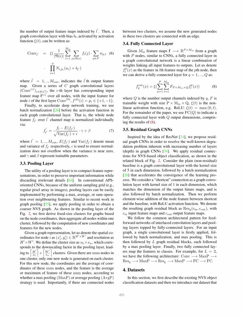
the number of output feature maps indexed by l′

. Then, a

graph convolution layer with bias bl, activated by activation

function ξ(t), can be written as:

Convl′ = ξ(1

|N(i)|

Min∑

l=1

∑

j∈N(i)

fl(j) ·∑

p∈P

wp,l (6)

·

d∏

i=1

Ni,pi(ui) + bl′ )

where l′

= 1, ..,Mout, indicates the l′

th output feature

map. Given a series of C graph convolutional layers

(Conv(c))c∈[0,C], the c-th layer has corresponding input

feature map f (c) over all nodes, with the input feature for

node i of the first layer Conv(0), f (0)(i) = pi ∈ {+1,−1}.

Finally, to accelerate deep network training, we use

batch normalization [26] before the activation function in

each graph convolutional layer. That is, the whole node

feature fl′ over l′

channel map is normalized individually

via:

f′

l′ =

fl − E(fl′ )√

Var(fl′ ) + ǫ· γ + β (7)

where l′

= 1, ..,Mout, E(fl′ ) and Var(fl′ ) denote mean

and variance of fl′ respectively, ǫ is used to ensure normal-

ization does not overflow when the variance is near zero,

and γ and β represent trainable parameters.

3.3. Pooling Layer

The utility of a pooling layer is to compact feature repre-

sentations, in order to preserve important information while

discarding irrelevant details [64]. In conventional APS-

oriented CNNs, because of the uniform sampling grid (e.g.,

regular pixel array in images), pooling layers can be easily

implemented by performing a max, average, or sum opera-

tion over neighbouring features. Similar to recent work in

graph pooling [55], we apply pooling in order to obtain a

coarser NVS graph. As shown in the pooling layer of the

Fig. 2, we first derive fixed-size clusters for graphs based

on the node coordinates, then aggregate all nodes within one

cluster, followed by the computation of new coordinates and

features for the new nodes.

Given a graph representation, let us denote the spatial co-

ordinates for node i as (x′i, y

′i) ∈ R

H′×W ′

and resolution as

H ′×W ′. We define the cluster size as sh×sw, which corre-

sponds to the downscaling factor in the pooling layer, lead-

ing to⌈

H′

sh

⌉

×⌈

W ′

sw

⌉

clusters. Given there are num nodes in

one cluster, only one new node is generated on each cluster.

For this new node, the coordinates are the average of coor-

dinates of these num nodes, and the feature is the average

or maximum of feature of these num nodes, according to

whether a max pooling (MaxP) or average pooling (AvgP)strategy is used. Importantly, if there are connected nodes

between two clusters, we assume the new generated nodes

in these two clusters are connected with an edge.

3.4. Fully Connected Layer

Given Min feature maps f −→ RP×Min from a graph

with P nodes, similar to CNNs, a fully connected layer in

a graph convolutional network is a linear combination of

weights linking all input features to outputs. Let us denote

fpl (x) as the feature in lth feature map of the pth node, then

we can derive a fully connected layer for q = 1, ..., Q as:

foutq (x) = ξ(

P∑

p=1

Min∑

l=1

FP×Min×Qfpl (x)) (8)

where Q is the number output channels indexed by q, F is

trainable weight with size P×Min ×Q, ξ(t) is the non-

linear activation function, e.g. ReLU: ξ(t) = max (0, t).For the remainder of the paper, we use FC(Q) to indicate a

fully connected layer with Q output dimensions, compris-

ing the results of (8).

3.5. Residual Graph CNNs

Inspired by the idea of ResNet [24], we propose resid-

ual graph CNNs in order to resolve the well-known degra-

dation problem inherent with increasing number of layers

(depth) in graph CNNs [34]. We apply residual connec-

tions for NVS-based object classification, as shown in the

related block of Fig. 2. Consider the plain (non-residual)

baseline is a graph convolutional layer with the kernel size

of 5 in each dimension, followed by a batch normalization

[26] that accelerates the convergence of the learning pro-

cess. We consider a “shortcut” connection as a graph convo-

lution layer with kernel size of 1 in each dimension, which

matches the dimension of the output future maps, and is

also followed by batch normalization. Then we perform

element-wise addition of the node feature between shortcut

and the baseline, with ReLU activation function. We denote

the resulting graph residual block as Resg(cin, cout), with

cin input feature maps and cout output feature maps.

We follow the common architectural pattern for feed-

forward networks of interlaced convolution layers and pool-

ing layers topped by fully-connected layers. For an input

graph, a single convolutional layer is firstly applied, fol-

lowed by batch normalization, and max pooling. This is

then followed by L graph residual blocks, each followed

by a max pooling layer. Finally, two fully connected lay-

ers map the features to classes. For example, for L = 2,

we have the following architecture: Conv −→ MaxP −→Resg −→ MaxP −→ Resg −→ MaxP −→ FC −→ FC.

4. Datasets

In this section, we first describe the existing NVS object

classification datasets and then we introduce our dataset that

495

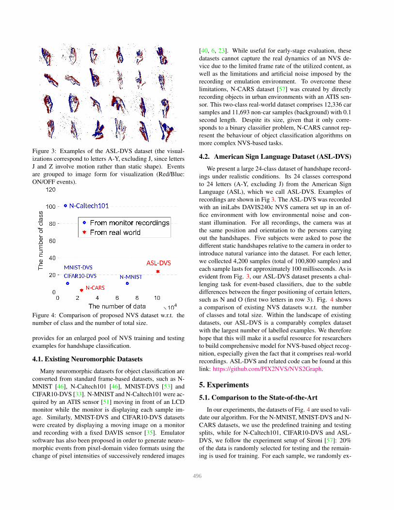
Figure 3: Examples of the ASL-DVS dataset (the visual-

izations correspond to letters A-Y, excluding J, since letters

J and Z involve motion rather than static shape). Events

are grouped to image form for visualization (Red/Blue:

ON/OFF events).

Figure 4: Comparison of proposed NVS dataset w.r.t. the

number of class and the number of total size.

provides for an enlarged pool of NVS training and testing

examples for handshape classification.

4.1. Existing Neuromorphic Datasets

Many neuromorphic datasets for object classification are

converted from standard frame-based datasets, such as N-

MNIST [46], N-Caltech101 [46], MNIST-DVS [53] and

CIFAR10-DVS [33]. N-MNIST and N-Caltech101 were ac-

quired by an ATIS sensor [51] moving in front of an LCD

monitor while the monitor is displaying each sample im-

age. Similarly, MNIST-DVS and CIFAR10-DVS datasets

were created by displaying a moving image on a monitor

and recording with a fixed DAVIS sensor [35]. Emulator

software has also been proposed in order to generate neuro-

morphic events from pixel-domain video formats using the

change of pixel intensities of successively rendered images

[40, 6, 23]. While useful for early-stage evaluation, these

datasets cannot capture the real dynamics of an NVS de-

vice due to the limited frame rate of the utilized content, as

well as the limitations and artificial noise imposed by the

recording or emulation environment. To overcome these

limitations, N-CARS dataset [57] was created by directly

recording objects in urban environments with an ATIS sen-

sor. This two-class real-world dataset comprises 12,336 car

samples and 11,693 non-car samples (background) with 0.1

second length. Despite its size, given that it only corre-

sponds to a binary classifier problem, N-CARS cannot rep-

resent the behaviour of object classification algorithms on

more complex NVS-based tasks.

4.2. American Sign Language Dataset (ASL­DVS)

We present a large 24-class dataset of handshape record-

ings under realistic conditions. Its 24 classes correspond

to 24 letters (A-Y, excluding J) from the American Sign

Language (ASL), which we call ASL-DVS. Examples of

recordings are shown in Fig 3. The ASL-DVS was recorded

with an iniLabs DAVIS240c NVS camera set up in an of-

fice environment with low environmental noise and con-

stant illumination. For all recordings, the camera was at

the same position and orientation to the persons carrying

out the handshapes. Five subjects were asked to pose the

different static handshapes relative to the camera in order to

introduce natural variance into the dataset. For each letter,

we collected 4,200 samples (total of 100,800 samples) and

each sample lasts for approximately 100 milliseconds. As is

evident from Fig. 3, our ASL-DVS dataset presents a chal-

lenging task for event-based classifiers, due to the subtle

differences between the finger positioning of certain letters,

such as N and O (first two letters in row 3). Fig. 4 shows

a comparison of existing NVS datasets w.r.t. the number

of classes and total size. Within the landscape of existing

datasets, our ASL-DVS is a comparably complex dataset

with the largest number of labelled examples. We therefore

hope that this will make it a useful resource for researchers

to build comprehensive model for NVS-based object recog-

nition, especially given the fact that it comprises real-world

recordings. ASL-DVS and related code can be found at this

link: https://github.com/PIX2NVS/NVS2Graph.

5. Experiments

5.1. Comparison to the State­of­the­Art

In our experiments, the datasets of Fig. 4 are used to vali-

date our algorithm. For the N-MNIST, MNIST-DVS and N-

CARS datasets, we use the predefined training and testing

splits, while for N-Caltech101, CIFAR10-DVS and ASL-

DVS, we follow the experiment setup of Sironi [57]: 20%

of the data is randomly selected for testing and the remain-

ing is used for training. For each sample, we randomly ex-

496

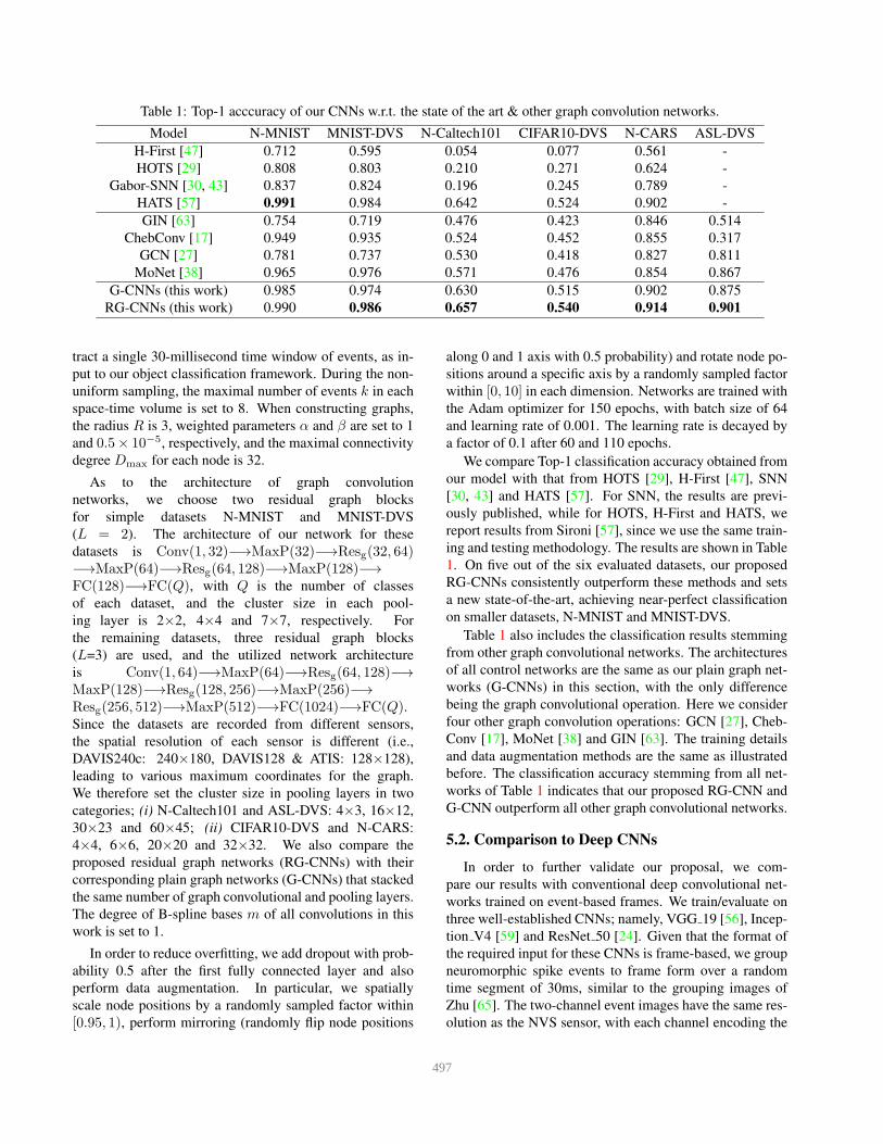
Table 1: Top-1 acccuracy of our CNNs w.r.t. the state of the art & other graph convolution networks.

Model N-MNIST MNIST-DVS N-Caltech101 CIFAR10-DVS N-CARS ASL-DVS

H-First [47] 0.712 0.595 0.054 0.077 0.561 -

HOTS [29] 0.808 0.803 0.210 0.271 0.624 -

Gabor-SNN [30, 43] 0.837 0.824 0.196 0.245 0.789 -

HATS [57] 0.991 0.984 0.642 0.524 0.902 -

GIN [63] 0.754 0.719 0.476 0.423 0.846 0.514

ChebConv [17] 0.949 0.935 0.524 0.452 0.855 0.317

GCN [27] 0.781 0.737 0.530 0.418 0.827 0.811

MoNet [38] 0.965 0.976 0.571 0.476 0.854 0.867

G-CNNs (this work) 0.985 0.974 0.630 0.515 0.902 0.875

RG-CNNs (this work) 0.990 0.986 0.657 0.540 0.914 0.901

tract a single 30-millisecond time window of events, as in-

put to our object classification framework. During the non-

uniform sampling, the maximal number of events k in each

space-time volume is set to 8. When constructing graphs,

the radius R is 3, weighted parameters α and β are set to 1

and 0.5× 10−5, respectively, and the maximal connectivity

degree Dmax for each node is 32.

As to the architecture of graph convolution

networks, we choose two residual graph blocks

for simple datasets N-MNIST and MNIST-DVS

(L = 2). The architecture of our network for these

datasets is Conv(1, 32)−→MaxP(32)−→Resg(32, 64)−→MaxP(64)−→Resg(64, 128)−→MaxP(128)−→FC(128)−→FC(Q), with Q is the number of classes

of each dataset, and the cluster size in each pool-

ing layer is 2×2, 4×4 and 7×7, respectively. For

the remaining datasets, three residual graph blocks

(L=3) are used, and the utilized network architecture

is Conv(1, 64)−→MaxP(64)−→Resg(64, 128)−→MaxP(128)−→Resg(128, 256)−→MaxP(256)−→Resg(256, 512)−→MaxP(512)−→FC(1024)−→FC(Q).Since the datasets are recorded from different sensors,

the spatial resolution of each sensor is different (i.e.,

DAVIS240c: 240×180, DAVIS128 & ATIS: 128×128),

leading to various maximum coordinates for the graph.

We therefore set the cluster size in pooling layers in two

categories; (i) N-Caltech101 and ASL-DVS: 4×3, 16×12,

30×23 and 60×45; (ii) CIFAR10-DVS and N-CARS:

4×4, 6×6, 20×20 and 32×32. We also compare the

proposed residual graph networks (RG-CNNs) with their

corresponding plain graph networks (G-CNNs) that stacked

the same number of graph convolutional and pooling layers.

The degree of B-spline bases m of all convolutions in this

work is set to 1.

In order to reduce overfitting, we add dropout with prob-

ability 0.5 after the first fully connected layer and also

perform data augmentation. In particular, we spatially

scale node positions by a randomly sampled factor within

[0.95, 1), perform mirroring (randomly flip node positions

along 0 and 1 axis with 0.5 probability) and rotate node po-

sitions around a specific axis by a randomly sampled factor

within [0, 10] in each dimension. Networks are trained with

the Adam optimizer for 150 epochs, with batch size of 64

and learning rate of 0.001. The learning rate is decayed by

a factor of 0.1 after 60 and 110 epochs.

We compare Top-1 classification accuracy obtained from

our model with that from HOTS [29], H-First [47], SNN

[30, 43] and HATS [57]. For SNN, the results are previ-

ously published, while for HOTS, H-First and HATS, we

report results from Sironi [57], since we use the same train-

ing and testing methodology. The results are shown in Table

1. On five out of the six evaluated datasets, our proposed

RG-CNNs consistently outperform these methods and sets

a new state-of-the-art, achieving near-perfect classification

on smaller datasets, N-MNIST and MNIST-DVS.

Table 1 also includes the classification results stemming

from other graph convolutional networks. The architectures

of all control networks are the same as our plain graph net-

works (G-CNNs) in this section, with the only difference

being the graph convolutional operation. Here we consider

four other graph convolution operations: GCN [27], Cheb-

Conv [17], MoNet [38] and GIN [63]. The training details

and data augmentation methods are the same as illustrated

before. The classification accuracy stemming from all net-

works of Table 1 indicates that our proposed RG-CNN and

G-CNN outperform all other graph convolutional networks.

5.2. Comparison to Deep CNNs

In order to further validate our proposal, we com-

pare our results with conventional deep convolutional net-

works trained on event-based frames. We train/evaluate on

three well-established CNNs; namely, VGG 19 [56], Incep-

tion V4 [59] and ResNet 50 [24]. Given that the format of

the required input for these CNNs is frame-based, we group

neuromorphic spike events to frame form over a random

time segment of 30ms, similar to the grouping images of

Zhu [65]. The two-channel event images have the same res-

olution as the NVS sensor, with each channel encoding the

497

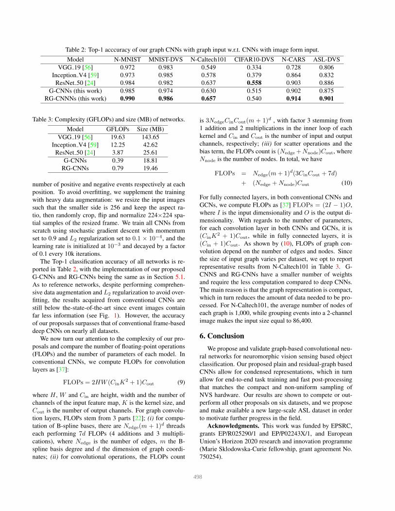
Table 2: Top-1 acccuracy of our graph CNNs with graph input w.r.t. CNNs with image form input.

Model N-MNIST MNIST-DVS N-Caltech101 CIFAR10-DVS N-CARS ASL-DVS

VGG 19 [56] 0.972 0.983 0.549 0.334 0.728 0.806

Inception V4 [59] 0.973 0.985 0.578 0.379 0.864 0.832

ResNet 50 [24] 0.984 0.982 0.637 0.558 0.903 0.886

G-CNNs (this work) 0.985 0.974 0.630 0.515 0.902 0.875

RG-CNNNs (this work) 0.990 0.986 0.657 0.540 0.914 0.901

Table 3: Complexity (GFLOPs) and size (MB) of networks.

Model GFLOPs Size (MB)

VGG 19 [56] 19.63 143.65

Inception V4 [59] 12.25 42.62

ResNet 50 [24] 3.87 25.61

G-CNNs 0.39 18.81

RG-CNNs 0.79 19.46

number of positive and negative events respectively at each

position. To avoid overfitting, we supplement the training

with heavy data augmentation: we resize the input images

such that the smaller side is 256 and keep the aspect ra-

tio, then randomly crop, flip and normalize 224×224 spa-

tial samples of the resized frame. We train all CNNs from

scratch using stochastic gradient descent with momentum

set to 0.9 and L2 regularization set to 0.1 × 10−4, and the

learning rate is initialized at 10−3 and decayed by a factor

of 0.1 every 10k iterations.

The Top-1 classification accuracy of all networks is re-

ported in Table 2, with the implementation of our proposed

G-CNNs and RG-CNNs being the same as in Section 5.1.

As to reference networks, despite performing comprehen-

sive data augmentation and L2 regularization to avoid over-

fitting, the results acquired from conventional CNNs are

still below the-state-of-the-art since event images contain

far less information (see Fig. 1). However, the accuracy

of our proposals surpasses that of conventional frame-based

deep CNNs on nearly all datasets.

We now turn our attention to the complexity of our pro-

posals and compare the number of floating-point operations

(FLOPs) and the number of parameters of each model. In

conventional CNNs, we compute FLOPs for convolution

layers as [37]:

FLOPs = 2HW (CinK2 + 1)Cout (9)

where H , W and Cin are height, width and the number of

channels of the input feature map, K is the kernel size, and

Cout is the number of output channels. For graph convolu-

tion layers, FLOPs stem from 3 parts [22]; (i) for compu-

tation of B-spline bases, there are Nedge(m + 1)d threads

each performing 7d FLOPs (4 additions and 3 multipli-

cations), where Nedge is the number of edges, m the B-

spline basis degree and d the dimension of graph coordi-

nates; (ii) for convolutional operations, the FLOPs count

is 3NedgeCinCout(m + 1)d , with factor 3 stemming from

1 addition and 2 multiplications in the inner loop of each

kernel and Cin and Cout is the number of input and output

channels, respectively; (iii) for scatter operations and the

bias term, the FLOPs count is (Nedge +Nnode)Cout, where

Nnode is the number of nodes. In total, we have

FLOPs = Nedge(m+ 1)d(3CinCout + 7d)

+ (Nedge +Nnode)Cout (10)

For fully connected layers, in both conventional CNNs and

GCNs, we compute FLOPs as [37] FLOPs = (2I − 1)O,

where I is the input dimensionality and O is the output di-

mensionality. With regards to the number of parameters,

for each convolution layer in both CNNs and GCNs, it is

(CinK2 + 1)Cout, while in fully connected layers, it is

(Cin + 1)Cout. As shown by (10), FLOPs of graph con-

volution depend on the number of edges and nodes. Since

the size of input graph varies per dataset, we opt to report

representative results from N-Caltech101 in Table 3. G-

CNNS and RG-CNNs have a smaller number of weights

and require the less computation compared to deep CNNs.

The main reason is that the graph representation is compact,

which in turn reduces the amount of data needed to be pro-

cessed. For N-Caltech101, the average number of nodes of

each graph is 1,000, while grouping events into a 2-channel

image makes the input size equal to 86,400.

6. Conclusion

We propose and validate graph-based convolutional neu-

ral networks for neuromorphic vision sensing based object

classification. Our proposed plain and residual-graph based

CNNs allow for condensed representations, which in turn

allow for end-to-end task training and fast post-processing

that matches the compact and non-uniform sampling of

NVS hardware. Our results are shown to compete or out-

perform all other proposals on six datasets, and we propose

and make available a new large-scale ASL dataset in order

to motivate further progress in the field.

Acknowledgments. This work was funded by EPSRC,

grants EP/R025290/1 and EP/P02243X/1, and European

Union’s Horizon 2020 research and innovation programme

(Marie Sklodowska-Curie fellowship, grant agreement No.

750254).

498

References

[1] Filipp Akopyan, Jun Sawada, Andrew Cassidy, Rodrigo

Alvarez-Icaza, John Arthur, Paul Merolla, Nabil Imam, Yu-

taka Nakamura, Pallab Datta, Gi-Joon Nam, et al. Truenorth:

Design and tool flow of a 65 mw 1 million neuron pro-

grammable neurosynaptic chip. IEEE Transactions on

Computer-Aided Design of Integrated Circuits and Systems,

34(10):1537–1557, 2015. 2

[2] James Atwood and Don Towsley. Diffusion-convolutional

neural networks. In Advances in Neural Information Pro-

cessing Systems, pages 1993–2001, 2016. 3

[3] Francisco Barranco, Cornelia Fermuller, and Yiannis Aloi-

monos. Contour motion estimation for asynchronous event-

driven cameras. Proceedings of the IEEE, 102(10):1537–

1556, 2014. 2

[4] Francisco Barranco, Cornelia Fermuller, and Yiannis Aloi-

monos. Bio-inspired motion estimation with event-driven

sensors. In International Work-Conference on Artificial Neu-

ral Networks, pages 309–321. Springer, 2015. 2

[5] Ryad Benosman, Charles Clercq, Xavier Lagorce, Sio-Hoi

Ieng, and Chiara Bartolozzi. Event-based visual flow.

IEEE transactions on neural networks and learning systems,

25(2):407–417, 2014. 2

[6] Yin Bi and Yiannis Andreopoulos. Pix2nvs: Parameterized

conversion of pixel-domain video frames to neuromorphic

vision streams. In 2017 IEEE International Conference on

Image Processing (ICIP), pages 1990–1994. IEEE, 2017. 2,

6

[7] Olivier Bichler, Damien Querlioz, Simon J Thorpe, Jean-

Philippe Bourgoin, and Christian Gamrat. Extraction of

temporally correlated features from dynamic vision sensors

with spike-timing-dependent plasticity. Neural Networks,

32:339–348, 2012. 2

[8] Davide Boscaini, Jonathan Masci, Emanuele Rodola, and

Michael Bronstein. Learning shape correspondence with

anisotropic convolutional neural networks. In Advances in

Neural Information Processing Systems, pages 3189–3197,

2016. 3, 4

[9] Michael M Bronstein, Joan Bruna, Yann LeCun, Arthur

Szlam, and Pierre Vandergheynst. Geometric deep learning:

going beyond euclidean data. IEEE Signal Processing Mag-

azine, 34(4):18–42, 2017. 4

[10] Tobias Brosch, Stephan Tschechne, and Heiko Neumann.

On event-based optical flow detection. Frontiers in neuro-

science, 9:137, 2015. 2

[11] Joan Bruna, Wojciech Zaremba, Arthur Szlam, and Yann Le-

Cun. Spectral networks and locally connected networks on

graphs. arXiv preprint arXiv:1312.6203, 2013. 3, 4

[12] Marco Cannici, Marco Ciccone, Andrea Romanoni, and

Matteo Matteucci. Attention mechanisms for object

recognition with event-based cameras. arXiv preprint

arXiv:1807.09480, 2018. 1, 2

[13] Marco Cannici, Marco Ciccone, Andrea Romanoni, and

Matteo Matteucci. Event-based convolutional networks for

object detection in neuromorphic cameras. arXiv preprint

arXiv:1805.07931, 2018. 1, 2

[14] Xavier Clady, Sio-Hoi Ieng, and Ryad Benosman. Asyn-

chronous event-based corner detection and matching. Neural

Networks, 66:91–106, 2015. 2

[15] Xavier Clady, Jean-Matthieu Maro, Sebastien Barre, and

Ryad B Benosman. A motion-based feature for event-based

pattern recognition. Frontiers in neuroscience, 10:594, 2017.

1, 2

[16] Gregory Kevin Cohen. Event-based feature detection, recog-

nition and classification. PhD thesis, Paris 6, 2016. 1, 2

[17] Michael Defferrard, Xavier Bresson, and Pierre Van-

dergheynst. Convolutional neural networks on graphs with

fast localized spectral filtering. In Advances in neural infor-

mation processing systems, pages 3844–3852, 2016. 3, 4,

7

[18] Tobi Delbruck. Neuromorphic vision sensing and process-

ing. In Europ. Solid-State Dev. Res. Conf, pages 7–14, 2016.

1

[19] Peter U Diehl and Matthew Cook. Unsupervised learning

of digit recognition using spike-timing-dependent plasticity.

Frontiers in computational neuroscience, 9:99, 2015. 2

[20] Peter U Diehl, Daniel Neil, Jonathan Binas, Matthew Cook,

Shih-Chii Liu, and Michael Pfeiffer. Fast-classifying, high-

accuracy spiking deep networks through weight and thresh-

old balancing. In 2015 International Joint Conference on

Neural Networks (IJCNN), pages 1–8. IEEE, 2015. 3

[21] David K Duvenaud, Dougal Maclaurin, Jorge Iparraguirre,

Rafael Bombarell, Timothy Hirzel, Alan Aspuru-Guzik, and

Ryan P Adams. Convolutional networks on graphs for learn-

ing molecular fingerprints. In Advances in neural informa-

tion processing systems, pages 2224–2232, 2015. 3

[22] Matthias Fey, Jan Eric Lenssen, Frank Weichert, and Hein-

rich Muller. Splinecnn: Fast geometric deep learning with

continuous b-spline kernels. In Proceedings of the IEEE

Conference on Computer Vision and Pattern Recognition,

pages 869–877, 2018. 3, 4, 8

[23] Garibaldi Pineda Garcıa, Patrick Camilleri, Qian Liu, and

Steve Furber. pydvs: An extensible, real-time dynamic

vision sensor emulator using off-the-shelf hardware. In

2016 IEEE Symposium Series on Computational Intelligence

(SSCI), pages 1–7. IEEE, 2016. 2, 6

[24] Kaiming He, Xiangyu Zhang, Shaoqing Ren, and Jian Sun.

Deep residual learning for image recognition. In Proceed-

ings of the IEEE conference on computer vision and pattern

recognition, pages 770–778, 2016. 1, 2, 5, 7, 8

[25] Yuhuang Hu, Hongjie Liu, Michael Pfeiffer, and Tobi Del-

bruck. Dvs benchmark datasets for object tracking, action

recognition, and object recognition. Frontiers in neuro-

science, 10:405, 2016. 2

[26] Sergey Ioffe and Christian Szegedy. Batch normalization:

Accelerating deep network training by reducing internal co-

variate shift. ICML, 2015. 5

[27] Thomas N Kipf and Max Welling. Semi-supervised classi-

fication with graph convolutional networks. ICLR, 2017. 3,

7

[28] Alex Krizhevsky, Ilya Sutskever, and Geoffrey E Hinton.

Imagenet classification with deep convolutional neural net-

works. In Advances in neural information processing sys-

tems, pages 1097–1105, 2012. 1

499

[29] Xavier Lagorce, Garrick Orchard, Francesco Galluppi,

Bertram E Shi, and Ryad B Benosman. Hots: a hierarchy

of event-based time-surfaces for pattern recognition. IEEE

transactions on pattern analysis and machine intelligence,

39(7):1346–1359, 2017. 1, 2, 7

[30] Jun Haeng Lee, Tobi Delbruck, and Michael Pfeiffer. Train-

ing deep spiking neural networks using backpropagation.

Frontiers in neuroscience, 10:508, 2016. 2, 7

[31] KH Lee, H Woo, and T Suk. Point data reduction using 3d

grids. The International Journal of Advanced Manufacturing

Technology, 18(3):201–210, 2001. 4

[32] Ron Levie, Federico Monti, Xavier Bresson, and Michael M

Bronstein. Cayleynets: Graph convolutional neural networks

with complex rational spectral filters. IEEE Transactions on

Signal Processing, 67(1):97–109, 2017. 3

[33] Hongmin Li, Hanchao Liu, Xiangyang Ji, Guoqi Li, and

Luping Shi. Cifar10-dvs: an event-stream dataset for ob-

ject classification. Frontiers in neuroscience, 11:309, 2017.

2, 6

[34] Qimai Li, Zhichao Han, and Xiao-Ming Wu. Deeper insights

into graph convolutional networks for semi-supervised learn-

ing. In Thirty-Second AAAI Conference on Artificial Intelli-

gence, 2018. 5

[35] Patrick Lichtsteiner, Christoph Posch, and Tobi Delbruck.

A 128x128, 120 db 30mw latency asynchronous temporal

contrast vision sensor. IEEE journal of solid-state circuits,

43(2):566–576, 2008. 6

[36] Jonathan Masci, Davide Boscaini, Michael Bronstein, and

Pierre Vandergheynst. Geodesic convolutional neural net-

works on riemannian manifolds. In Proceedings of the

IEEE international conference on computer vision work-

shops, pages 37–45, 2015. 3, 4

[37] Pavlo Molchanov, Stephen Tyree, Tero Karras, Timo Aila,

and Jan Kautz. Pruning convolutional neural networks for

resource efficient inference. ICLR, 2017. 8

[38] Federico Monti, Davide Boscaini, Jonathan Masci,

Emanuele Rodola, Jan Svoboda, and Michael M Bronstein.

Geometric deep learning on graphs and manifolds using

mixture model cnns. In Proceedings of the IEEE Confer-

ence on Computer Vision and Pattern Recognition, pages

5115–5124, 2017. 3, 4, 7

[39] Elias Mueggler, Chiara Bartolozzi, and Davide Scaramuzza.

Fast event-based corner detection. In British Machine Vis.

Conf.(BMVC), volume 1, 2017. 2

[40] Elias Mueggler, Henri Rebecq, Guillermo Gallego, Tobi Del-

bruck, and Davide Scaramuzza. The event-camera dataset

and simulator: Event-based data for pose estimation, visual

odometry, and slam. The International Journal of Robotics

Research, 36(2):142–149, 2017. 2, 6

[41] Emre Neftci, Srinjoy Das, Bruno Pedroni, Kenneth Kreutz-

Delgado, and Gert Cauwenberghs. Event-driven contrastive

divergence for spiking neuromorphic systems. Frontiers in

neuroscience, 7:272, 2014. 2

[42] E Neftci, C Posch, E Chicca, and H Ishibuchi. Neuromorphic

engineering. Computational Intelligence, 2:278, 2015. 1

[43] Daniel Neil, Michael Pfeiffer, and Shih-Chii Liu. Phased

lstm: Accelerating recurrent network training for long or

event-based sequences. In Advances in Neural Information

Processing Systems, pages 3882–3890, 2016. 7

[44] Peter O’Connor, Daniel Neil, Shih-Chii Liu, Tobi Delbruck,

and Michael Pfeiffer. Real-time classification and sensor fu-

sion with a spiking deep belief network. Frontiers in neuro-

science, 7:178, 2013. 3

[45] Garrick Orchard and Ralph Etienne-Cummings. Bioin-

spired visual motion estimation. Proceedings of the IEEE,

102(10):1520–1536, 2014. 2

[46] Garrick Orchard, Ajinkya Jayawant, Gregory K Cohen, and

Nitish Thakor. Converting static image datasets to spiking

neuromorphic datasets using saccades. Frontiers in neuro-

science, 9:437, 2015. 6

[47] Garrick Orchard, Cedric Meyer, Ralph Etienne-Cummings,

Christoph Posch, Nitish Thakor, and Ryad Benosman.

Hfirst: a temporal approach to object recognition. IEEE

transactions on pattern analysis and machine intelligence,

37(10):2028–2040, 2015. 7

[48] Xi Peng, Bo Zhao, Rui Yan, Huajin Tang, and Zhang Yi. Bag

of events: an efficient probability-based feature extraction

method for aer image sensors. IEEE transactions on neural

networks and learning systems, 28(4):791–803, 2017. 2

[49] Jose Antonio Perez-Carrasco, Bo Zhao, Carmen Serrano,

Begona Acha, Teresa Serrano-Gotarredona, Shouchun Chen,

and Bernabe Linares-Barranco. Mapping from frame-driven

to frame-free event-driven vision systems by low-rate rate

coding and coincidence processing–application to feedfor-

ward convnets. IEEE transactions on pattern analysis and

machine intelligence, 35(11):2706–2719, 2013. 3

[50] Les Piegl and Wayne Tiller. The NURBS book. Springer

Science & Business Media, 2012. 4

[51] Christoph Posch, Daniel Matolin, and Rainer Wohlgenannt.

A qvga 143 db dynamic range frame-free pwm image sensor

with lossless pixel-level video compression and time-domain

cds. IEEE Journal of Solid-State Circuits, 46(1):259–275,

2011. 1, 6

[52] Aliaksei Sandryhaila and Jose MF Moura. Discrete signal

processing on graphs. IEEE transactions on signal process-

ing, 61(7):1644–1656, 2013. 3, 4

[53] Teresa Serrano-Gotarredona and Bernabe Linares-Barranco.

Poker-dvs and mnist-dvs. their history, how they were made,

and other details. Frontiers in neuroscience, 9:481, 2015. 2,

6

[54] David I Shuman, Sunil K Narang, Pascal Frossard, Anto-

nio Ortega, and Pierre Vandergheynst. The emerging field

of signal processing on graphs: Extending high-dimensional

data analysis to networks and other irregular domains. arXiv

preprint arXiv:1211.0053, 2012. 3, 4

[55] Martin Simonovsky and Nikos Komodakis. Dynamic edge-

conditioned filters in convolutional neural networks on

graphs. In Proceedings of the IEEE Conference on Computer

Vision and Pattern Recognition, pages 3693–3702, 2017. 5

[56] Karen Simonyan and Andrew Zisserman. Very deep convo-

lutional networks for large-scale image recognition. arXiv

preprint arXiv:1409.1556, 2014. 7, 8

[57] Amos Sironi, Manuele Brambilla, Nicolas Bourdis, Xavier

Lagorce, and Ryad Benosman. Hats: histograms of aver-

500

aged time surfaces for robust event-based object classifica-

tion. In Proceedings of the IEEE Conference on Computer

Vision and Pattern Recognition, pages 1731–1740, 2018. 1,

2, 6, 7

[58] Evangelos Stromatias, Daniel Neil, Francesco Galluppi,

Michael Pfeiffer, Shih-Chii Liu, and Steve Furber. Scal-

able energy-efficient, low-latency implementations of trained

spiking deep belief networks on spinnaker. In 2015 Interna-

tional Joint Conference on Neural Networks (IJCNN), pages

1–8. IEEE, 2015. 3

[59] Christian Szegedy, Sergey Ioffe, Vincent Vanhoucke, and

Alexander A Alemi. Inception-v4, inception-resnet and the

impact of residual connections on learning. In Thirty-First

AAAI Conference on Artificial Intelligence, 2017. 7, 8

[60] Cheston Tan, Stephane Lallee, and Garrick Orchard. Bench-

marking neuromorphic vision: lessons learnt from computer

vision. Frontiers in neuroscience, 9:374, 2015. 1

[61] Valentina Vasco, Arren Glover, and Chiara Bartolozzi. Fast

event-based harris corner detection exploiting the advantages

of event-driven cameras. In 2016 IEEE/RSJ International

Conference on Intelligent Robots and Systems (IROS), pages

4144–4149. IEEE, 2016. 2

[62] Chu Wang, Babak Samari, and Kaleem Siddiqi. Local spec-

tral graph convolution for point set feature learning. In Pro-

ceedings of the European Conference on Computer Vision

(ECCV), pages 52–66, 2018. 3, 4

[63] Keyulu Xu, Weihua Hu, Jure Leskovec, and Stefanie Jegelka.

How powerful are graph neural networks? ICLR, 2019. 7

[64] Fan Yang, Wongun Choi, and Yuanqing Lin. Exploit all the

layers: Fast and accurate cnn object detector with scale de-

pendent pooling and cascaded rejection classifiers. In Pro-

ceedings of the IEEE conference on computer vision and pat-

tern recognition, pages 2129–2137, 2016. 5

[65] Alex Zihao Zhu, Liangzhe Yuan, Kenneth Chaney, and

Kostas Daniilidis. Ev-flownet: self-supervised optical

flow estimation for event-based cameras. arXiv preprint

arXiv:1802.06898, 2018. 1, 2, 7

501