Sampling-free Epistemic Uncertainty Estimation Using Approximated Variance

Propagation

Janis Postels1,2 Francesco Ferroni2 Huseyin Coskun1 Nassir Navab1 Federico Tombari1,3

1Technical University Munich 2Autonomous Intelligent Driving GmbH 3Google

{janis.postels, huseyin.coskun, nassir.navab}@tum.de francesco.ferroni@aid-driving.eu

tombari@in.tum.de

Abstract

We present a sampling-free approach for computing the

epistemic uncertainty of a neural network. Epistemic uncer-

tainty is an important quantity for the deployment of deep

neural networks in safety-critical applications, since it rep-

resents how much one can trust predictions on new data.

Recently promising works were proposed using noise in-

jection combined with Monte-Carlo (MC) sampling at in-

ference time to estimate this quantity (e.g. MC dropout).

Our main contribution is an approximation of the epistemic

uncertainty estimated by these methods that does not re-

quire sampling, thus notably reducing the computational

overhead. We apply our approach to large-scale visual

tasks (i.e., semantic segmentation and depth regression) to

demonstrate the advantages of our method compared to

sampling-based approaches in terms of quality of the un-

certainty estimates as well as of computational overhead.

1. Introduction

Quantifying the uncertainty associated with the predic-

tion of neural networks is a prerequisite for their deploy-

ment and use in safety-critical applications. Whether used

to detect road users and make driving decisions in an au-

tonomous vehicle, or in a medical setting within a surgical

robot, neural networks must be able not just to predict ac-

curately, but also to quantify how certain they are regarding

predictions. Moreover, it is important that uncertainty is

provided during inference in real-time, so that the uncer-

tainty can be exploited by a real-time safety-critical system.

One can estimate two types of uncertainty of a machine

learning model [8]: aleatoric and epistemic. Aleatoric un-

certainty is inherent to the data itself, e.g. uncertainty re-

sulting from noisy sensors. This type of uncertainty can

be incorporated into the deep model itself by applying e.g.

mixture density networks [2]. Epistemic uncertainty is the

uncertainty in the chosen model parameters. In order to

detect situations which are unfamiliar for a given machine

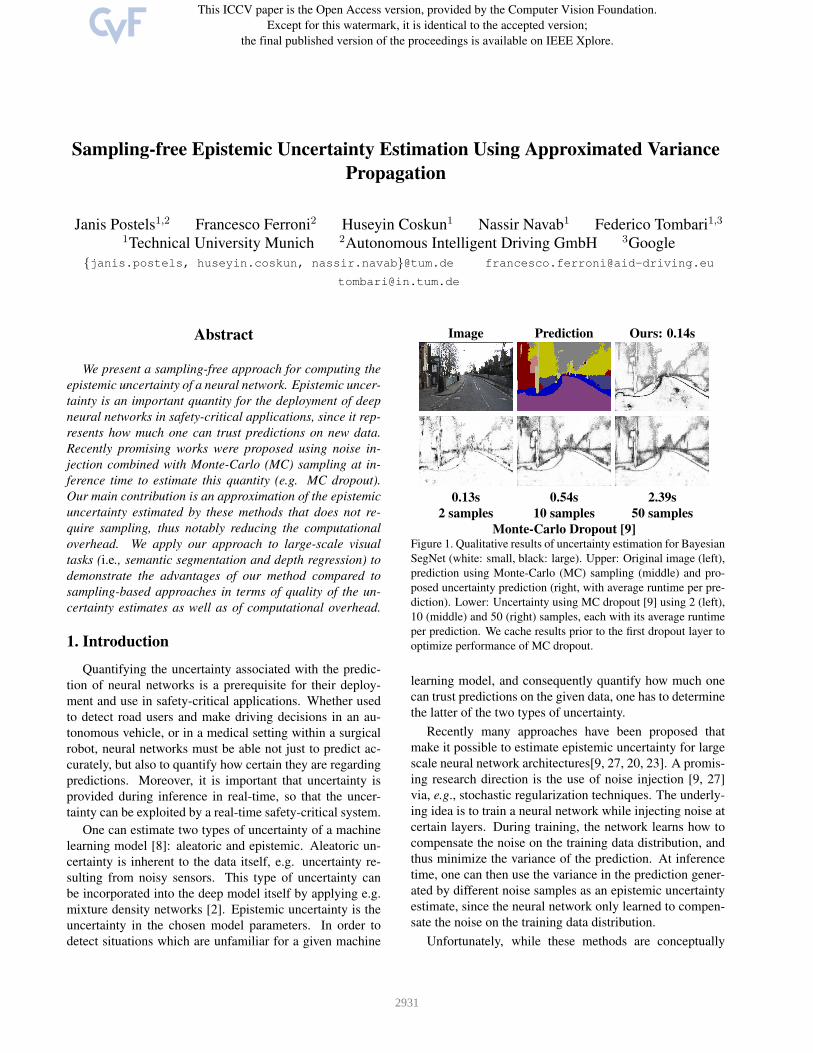
Image Prediction Ours: 0.14s

0.13s 0.54s 2.39s

2 samples 10 samples 50 samples

Monte-Carlo Dropout [9]Figure 1. Qualitative results of uncertainty estimation for Bayesian

SegNet (white: small, black: large). Upper: Original image (left),

prediction using Monte-Carlo (MC) sampling (middle) and pro-

posed uncertainty prediction (right, with average runtime per pre-

diction). Lower: Uncertainty using MC dropout [9] using 2 (left),

10 (middle) and 50 (right) samples, each with its average runtime

per prediction. We cache results prior to the first dropout layer to

optimize performance of MC dropout.

learning model, and consequently quantify how much one

can trust predictions on the given data, one has to determine

the latter of the two types of uncertainty.

Recently many approaches have been proposed that

make it possible to estimate epistemic uncertainty for large

scale neural network architectures[9, 27, 20, 23]. A promis-

ing research direction is the use of noise injection [9, 27]

via, e.g., stochastic regularization techniques. The underly-

ing idea is to train a neural network while injecting noise at

certain layers. During training, the network learns how to

compensate the noise on the training data distribution, and

thus minimize the variance of the prediction. At inference

time, one can then use the variance in the prediction gener-

ated by different noise samples as an epistemic uncertainty

estimate, since the neural network only learned to compen-

sate the noise on the training data distribution.

Unfortunately, while these methods are conceptually

2931

simple and have been successful in delivering a measure

of epistemic uncertainty for neural networks (even large

architectures, e.g. [18, 10, 1]), they rely on MC sam-

pling at inference time in order to determine the variance of

the prediction as an uncertainty estimate. This means that

computation time scales linearly with the number of sam-

ples, and therefore, can become prohibitively expensive for

performance-critical or compute-limited applications, such

as autonomous vehicles, robots and mobile devices. In such

cases, obtaining epistemic uncertainty as part of a model

prediction can be a functional safety requirement, but the

need to perform real-time inference from sensor data makes

MC dropout a difficult proposition.

In this work, we side-step these issues and produce epis-

temic uncertainty estimates of a neural network’s prediction

which are at the same time accurate and computationally in-

expensive. Our contributions are specifically:

• A sampling-free approach to approximate uncertainty

estimates that rely on noise injection at training time.

• Further simplification specifically for convolutional

neural networks using ReLU activation functions.

Subsequently, we will first outline relevant work, sec-

ondly present our sampling-free framework and finally

show experimental results. Specifically, we compare the

quality of our approximation to Bayesian SegNet [18] on

CamVid dataset [4], and show the ability of our approx-

imation to detect out-of-distribution samples by training

Bayesian SegNet only on a subset of classes. We further

apply our approximation in a common regression task for

computer vision, i.e. monocular depth estimation [12].

We release all code used for this work1.

2. Related Work

Recently there has been a wealth of proposals regarding

epistemic uncertainty estimation for large-scale neural net-

works [3, 14, 23, 20, 9, 27, 31, 22, 24]. The common goal is

to approximate the full posterior distribution of the param-

eters of a neural network.

Some works aim to directly learn the parameters of a

family of distributions within back-propagation [31, 3, 14].

Another line of research approximates the posterior by

training ensembles of neural networks via random changes

in the training setup [23, 20] estimating the target distribu-

tion by an ensemble of sample distributions [6].

A different research avenue utilizes stochastic regular-

ization methods to estimate epistemic uncertainty at infer-

ence time [9, 27, 31]. The most prominent example is MC

dropout [9] - train a dropout regularized neural network, and

then, at inference time, keep dropout turned on to estimate

1https://github.com/janisgp/Sampling-free-Epistemic-Uncertainty

the epistemic uncertainty via the variance of the prediction.

These approaches have gained popularity due to the sim-

plicity with which they integrate into the current training

methodology. Consequently they have been applied to a va-

riety of tasks [10, 1, 18, 7, 17]. Despite their achievements,

they still suffer from large computational overhead at infer-

ence time due to sampling, which makes them prohibitively

expensive in applications that demand real-time inference

from large neural networks.

[15] optimizes the application of MC dropout on videos.

Therefore the authors treat images which are close in time

as constant, and thus samples of the same scene. Conse-

quently each image only has to be processed once while

performing approximate MC sampling.

Sampling-free estimation of epistemic uncertainty has

been only partially covered in literature. [5] incorpo-

rates sampling-free epistemic uncertainty into mixture den-

sity networks, which, following [21], suffers from non-

convergence for high dimensional problems. Natural Pa-

rameter Networks [28, 16] can be considered related to our

work. Instead of processing point estimates through a neu-

ral network, the authors adjust the transformations at each

layer to propagate the natural parameters of a pre-defined

distribution, e.g. mean and standard deviation of a Gaus-

sian. Our approach mainly differs from [28] due to the fol-

lowing two points. Firstly, [28] requires all operations to

preserve (approximately) the exponential family of distri-

butions. This constraints the architecture (e.g. one cannot

apply batch normalization/softmax due to inverse distribu-

tions). On the contrary, we explicitly do not alter the train-

ing procedure and the Jacobian-based propagation of un-

certainty allows practically every transformation. Secondly,

[28] assumes independent activations which our general ap-

proach does not. Thus we will not compare against this

work, as we are interested in approaches applicable to arbi-

trary neural networks without altering the training process.

[30] concurrently proposed sampling-free variational in-

ference. Our work differs by leaving the training unchanged

and only propagating uncertainties at test time. Hence, it

can be applied to any network with any loss function using

a stochastic process at training time, compared with [30],

which thus far only implements a simple regression setting.

We stress that our results on the UCI regression datasets are

not comparable with [30], since we only approximate sam-

pling at test time. Thus, our performance is upper bounded

by the corresponding MC method (e.g. MC dropout).

3. Method

Our goal is to estimate the epistemic uncertainty of a

neural network trained with injected noise at inference time

to quantify the level of trust in the predictions, in a single

shot. Note, that our method (OUR) leaves the training un-

changed. At its core OUR uses error propagation [26], com-

2932

A (A,B)f

1

C

D

E

B (A,B)f

2

(C,D)f

3

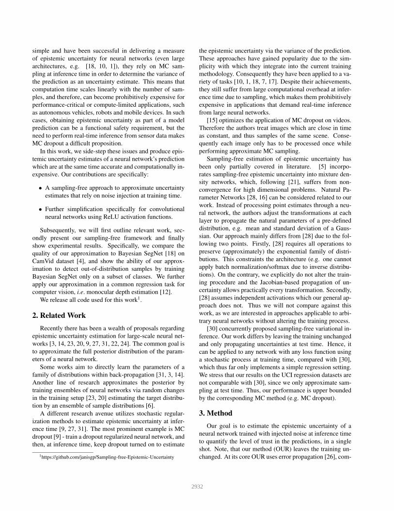
Figure 2. Computational graph for illustrating error propagation.

monly used in physics, where the error is equivalent to the

variance. We treat the noise injected in a neural network as

errors on the activation values. By training with noise in-

jection, the network implicitly learns to minimize the accu-

mulated errors on the training data distribution, since larger

errors correspond to large loss signals. To give an intuition

for this, we consider a simple computational graph (see Fig.

2). Let A and B be independent random variables and let

C = f1(A,B) and D = f2(A,B) be, possibly non-linear,

functions of A and B. Knowing the mean and the variance

σ2

A/B of A and B, we want to compute the variance of C

and D. We apply error propagation, where:

σ2

C/D =

(

∂f1/2

∂A

)2

σ2

A +

(

∂f1/2

∂B

)2

σ2

B (1)

Note that the partial derivatives only approximate the

outcome given non-linear functions f1/2. Let us assume

now that we have another function E = f3(C,D). We

cannot apply Eq. 1 directly to determine the variance of

E because C and D, unlike A and B, are not statistically in-

dependent. Thus we have to consider the full covariance

matrix of C and D which we can obtain again by apply-

ing error propagation. We start with the covariance matrix

ΣA,B of A and B. This is a diagonal matrix with entries σ2

A

and σ2

B on its main diagonal. Then we can approximate the

covariance matrix over C and D by computing:

ΣC,D = JTΣA,BJ (2)

J is the Jacobian of the vector-valued function ~f =(f1(A,B), f2(A,B))T . The variance σ2

E of E is obtained

by applying Eq. 2 considering that f3 is not a vector-valued

function. Thus one can exchange the Jacobian with the gra-

dient J = ∇C,Df3(C,D) = ( ∂∂C , ∂

∂D )T f3(C,D).This minimal example already illustrates all the tools we

need to approximate the variance at the output layer of a

neural network given some noise layer, such as dropout or

batch-norm [27] by applying error propagation. In the fol-

lowing, we explain the propagation of covariance for spe-

cific parts of a neural network: noise layers, affine lay-

ers, and non-linearities. Afterwards, we simplify the above

equations for the common setup of a convolution and ReLU

activation. This is necessary for high dimensional feature

spaces due to the size of the covariance matrix (which scales

quadratically with the number of activations).

Note that the propagation of the mean is unchanged.

Thus, given e.g. dropout, we apply the usual inference

scheme by scaling activations. We explore variance prop-

agation using error progation and leave adjusting the mean

propagation to future work. The nature of the uncer-

tainty estimate produced by OUR is inherited from MC

dropout. Consequently, it mainly models epistemic uncer-

tainty (though partially also aleatoric uncertainty)[19].

In the following X and Z denote random variables and~X and ~Z denote random vectors. Superscripts correspond

to layers, thus ~Xi is the random vector representing the ac-

tivations at layer i. Further Σ ~X /V ar[ ~X] denote the covari-

ance matrix/variance (main diagonal of Σ ~X ) of ~X .

3.1. Noise Layer

We derive the covariance matrix of a noise layer’s acti-

vation values. The following is independent of the imple-

mentation of the noise layer. We assume independent noise

across the nodes of the noise layer which is not a necessity

but common practice. In the following, superscripts corre-

spond to layers and subscripts to nodes within a layer.

Consider a neural network with l layers and N noise lay-

ers at positions i ∈ [0, l], where l = 0 denotes the input. Let

the input to a noise layer be a random vector ~Xi−1 with

covariance matrix Σ ~Xi−1 at layer i-1. Furthermore, let the

random vector representing the noise be ~Z ∈ Rn with a di-

agonal covariance matrix Σ~Z , where the entries of ~Z are in-

dependent and the entries of ~Xi−1 are generally dependent.

There are two ways how the noise is commonly injected:

addition and element-wise multiplication of ~Xi−1 and ~Z.

When the noise is injected by adding the random vectors,

the resulting covariance at layer i is simply given by

Σ ~Xi = Σ ~Xi−1 +Σ~Z (3)

When the noise injection resembles an element-wise

multiplication of the random vectors ~Xi−1 and ~Z (e.g.

dropout), the covariance matrix at layer i is given by [13]

Σi = Σ~Z◦ ~Xi−1, ~Z◦ ~Xi−1 = Σ~Z ◦ Σ ~Xi−1

+ E[~Z]E[~Z]T ◦ Σ ~Xi−1 + E[ ~Xi−1]E[ ~Xi−1]T ◦ Σ~Z (4)

where ◦ is the Hadamard product. We refer to the supple-

mentary material for a detailed derivation of this formula.

For the special case of the first noise layer in the network,

we can either model the input noise from prior knowledge

(i.e. sensor noise) or simplify it by assuming zero noise.

In the latter case, the resulting covariance matrix will be

diagonal given independent noise, resulting in:

Σ ~Xi = diag(σ2

0, ..., σ2

n) (5)

where n is the dimensionality of the activation vector and σ2

i

is the variance of activation i. The variance introduced by

the regular dropout, which follows a Bernoulli distribution,

is given by p(1− p)a2i , with p defining the dropout rate and

ai the mean activation of node i.

2933

3.2. Affine Layers and Non­Linearities

After obtaining the covariance matrix of a noise layer,

we propagate it to the output layer. This means applying a

series of affine layers and non-linearities. Here, we detail

the case of a fully-connected and convolutional layer. It is

straightforward to apply Eq. 2, given that for the transfor-

mation of an affine layer the Jacobian J equals the weight

matrix W. The covariance matrix is therefore,

Σ ~Xi = WΣ ~Xi−1WT (6)

This is an exact transformation which does not depend on

the underlying distribution. For the non-linearities in a neu-

ral network we approximate the transformation by a first-

order Taylor expansion. The covariance transformation at a

non-linearity is then given by:

Σ ~Xi ≈ JΣ ~Xi−1JT (7)

The particular Jacobians of the activation functions used

in our experiments (ReLU, sigmoid and softmax) can be

found in the supplementary material where we also provide

an analysis of the error introduced by the first-order Taylor

expansion of the softmax activation function.

3.3. Special Case: Convolutional Layers combinedwith ReLU Activations

Though the proposed approach does not require sam-

pling, propagating the full covariance matrix may become

prohibitively expensive for very high dimensional prob-

lems, such as images. This can be understood by consid-

ering that our method requires the full covariance matrix

Σ ∈ RN×N at each layer with N nodes. This leads to

a memory complexity of O(N2). Since the many neural

network architecture contains iterative applications of con-

volutional layers and rectified linear units, we simplify the

above formulas for the sake of computational efficiency.

For a fully connected layer, since each of its output nodes

is a linear combination of all input nodes, modeling the full

covariance is a necessity. However, this is not the case for

a convolutional layer which strength comes from sharing

weights across the entire input space and consequently ap-

plying a linear transformation only to a local neighborhood

of each pixel. For the following approximation we assume

a convolutional layer with kernel K ∈ RW

′

×H′

×C′

and

an input to the convolutional layer I ∈ RW×H×C with

W′

≪ W and H′

≪ H . Given a diagonal covariance

matrix prior to the convolutional layer, by applying e.g. a

dropout layer, the output covariance would be a sparse ma-

trix with a few non-zero entries off the main diagonal for

local neighbourhoods in the input space. This is illustrated

in Fig. 3 using a convolutional architecture on CIFAR10.

Furthermore, given approximately symmetrical distributed

weights ReLU activation leads to a probability of roughly

0.5 with which a variance value is dropped. This results in

the observed decrease in the mean variance with the number

of convolutional layers using ReLU activation functions.

The observation that this architectural setup does not trans-

port significant mass to wide regions of the covariance ma-

trix motivates us to assume a diagonal covariance matrix.

As a result the computational complexity of propagating

the variance reduces to the same level of normal forward

propagation because one only needs to propagate the vector

of the main diagonal of the covariance matrix. Under this

assumption Eq. 4 simplifies to:

V ar[ ~Xi] = E[ ~Xi−1]2 ◦ V ar[~Z]+

E[~Z]2 ◦ V ar[ ~Xi−1] + V ar[ ~Xi−1] ◦ V ar[~Z] (8)

Here V ar[ ~Xi] denotes the variance of the random vec-

tor ~Xi, thus the main diagonal of its covariance matrix. A

derivation can be found in the supplementary material.

To determine variances under the transformation of

weight matrices and Jacobians of non-linearities using the

above simplification, we need to square the corresponding

matrix element-wise and multiply it with the vector repre-

senting the main diagonal of the covariance matrix:

V ar[ ~Xi] = (W 2)V ar[ ~Xi−1] (9)

and respectively

V ar[ ~Xi] ≈ (J2)V ar[ ~Xi−1] (10)

Assuming independent activations, it is straightforward

to improve upon the Jacobian approximation of ReLU by

explicitly computing the variance resulting from applying

ReLU to a Gaussian. Therefore we assume a Gaussian dis-

tribution of activations prior to ReLU. The respective for-

mulas can be found in the supplementary material.

By assuming Gaussian distributed activations we

follow[29]. The authors argue that the output of an

affine layer with weights, unimodal distributed and cen-

tered around 0, and incoming activations, either unimodal

or in a fixed interval, is approximately Gaussian. [30] draws

the same conclusion while explicitly extending it to weakly

correlated activations. According to [29] this assumption

breaks when individual summands dominate the sum in the

affine operation (e.g. unnormalized data with one dimen-

sion having much larger magnitude than the rest).

4. Experiments

In this section we provide experimental evidence that

OUR can produce fast and accurate uncertainty estimates

in a classification and regression setting.

2934

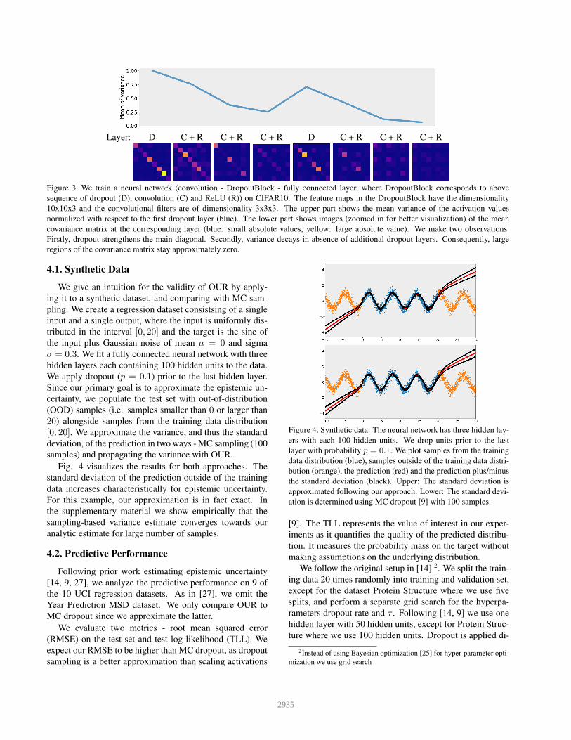
Layer: D C + R C + R C + R D C + R C + R C + R

Figure 3. We train a neural network (convolution - DropoutBlock - fully connected layer, where DropoutBlock corresponds to above

sequence of dropout (D), convolution (C) and ReLU (R)) on CIFAR10. The feature maps in the DropoutBlock have the dimensionality

10x10x3 and the convolutional filters are of dimensionality 3x3x3. The upper part shows the mean variance of the activation values

normalized with respect to the first dropout layer (blue). The lower part shows images (zoomed in for better visualization) of the mean

covariance matrix at the corresponding layer (blue: small absolute values, yellow: large absolute value). We make two observations.

Firstly, dropout strengthens the main diagonal. Secondly, variance decays in absence of additional dropout layers. Consequently, large

regions of the covariance matrix stay approximately zero.

4.1. Synthetic Data

We give an intuition for the validity of OUR by apply-

ing it to a synthetic dataset, and comparing with MC sam-

pling. We create a regression dataset consistsing of a single

input and a single output, where the input is uniformly dis-

tributed in the interval [0, 20] and the target is the sine of

the input plus Gaussian noise of mean µ = 0 and sigma

σ = 0.3. We fit a fully connected neural network with three

hidden layers each containing 100 hidden units to the data.

We apply dropout (p = 0.1) prior to the last hidden layer.

Since our primary goal is to approximate the epistemic un-

certainty, we populate the test set with out-of-distribution

(OOD) samples (i.e. samples smaller than 0 or larger than

20) alongside samples from the training data distribution

[0, 20]. We approximate the variance, and thus the standard

deviation, of the prediction in two ways - MC sampling (100

samples) and propagating the variance with OUR.

Fig. 4 visualizes the results for both approaches. The

standard deviation of the prediction outside of the training

data increases characteristically for epistemic uncertainty.

For this example, our approximation is in fact exact. In

the supplementary material we show empirically that the

sampling-based variance estimate converges towards our

analytic estimate for large number of samples.

4.2. Predictive Performance

Following prior work estimating epistemic uncertainty

[14, 9, 27], we analyze the predictive performance on 9 of

the 10 UCI regression datasets. As in [27], we omit the

Year Prediction MSD dataset. We only compare OUR to

MC dropout since we approximate the latter.

We evaluate two metrics - root mean squared error

(RMSE) on the test set and test log-likelihood (TLL). We

expect our RMSE to be higher than MC dropout, as dropout

sampling is a better approximation than scaling activations

Figure 4. Synthetic data. The neural network has three hidden lay-

ers with each 100 hidden units. We drop units prior to the last

layer with probability p = 0.1. We plot samples from the training

data distribution (blue), samples outside of the training data distri-

bution (orange), the prediction (red) and the prediction plus/minus

the standard deviation (black). Upper: The standard deviation is

approximated following our approach. Lower: The standard devi-

ation is determined using MC dropout [9] with 100 samples.

[9]. The TLL represents the value of interest in our exper-

iments as it quantifies the quality of the predicted distribu-

tion. It measures the probability mass on the target without

making assumptions on the underlying distribution.

We follow the original setup in [14] 2. We split the train-

ing data 20 times randomly into training and validation set,

except for the dataset Protein Structure where we use five

splits, and perform a separate grid search for the hyperpa-

rameters dropout rate and τ . Following [14, 9] we use one

hidden layer with 50 hidden units, except for Protein Struc-

ture where we use 100 hidden units. Dropout is applied di-

2Instead of using Bayesian optimization [25] for hyper-parameter opti-

mization we use grid search

2935

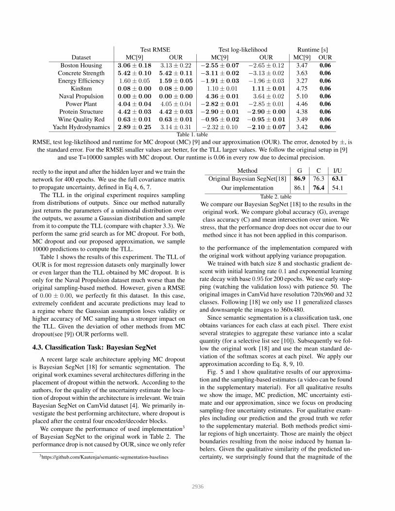
Test RMSE Test log-likelihood Runtime [s]

Dataset MC[9] OUR MC[9] OUR MC[9] OUR

Boston Housing 3.06± 0.18 3.13± 0.22 −2.55± 0.07 −2.65± 0.12 3.47 0.06

Concrete Strength 5.42± 0.10 5.42± 0.11 −3.11± 0.02 −3.13± 0.02 3.63 0.06

Energy Efficiency 1.60± 0.05 1.59± 0.05 −1.91± 0.03 −1.96± 0.03 3.27 0.06

Kin8nm 0.08± 0.00 0.08± 0.00 1.10± 0.01 1.11± 0.01 4.75 0.06

Naval Propulsion 0.00± 0.00 0.00± 0.00 4.36± 0.01 3.64± 0.02 5.10 0.06

Power Plant 4.04± 0.04 4.05± 0.04 −2.82± 0.01 −2.85± 0.01 4.46 0.06

Protein Structure 4.42± 0.03 4.42± 0.03 −2.90± 0.01 −2.90± 0.00 4.38 0.06

Wine Quality Red 0.63± 0.01 0.63± 0.01 −0.95± 0.02 −0.95± 0.01 3.49 0.06

Yacht Hydrodynamics 2.89± 0.25 3.14± 0.31 −2.32± 0.10 −2.10± 0.07 3.42 0.06Table 1. table

RMSE, test log-likelihood and runtime for MC dropout (MC) [9] and our approximation (OUR). The error, denoted by ±, is

the standard error. For the RMSE smaller values are better, for the TLL larger values. We follow the original setup in [9]

and use T=10000 samples with MC dropout. Our runtime is 0.06 in every row due to decimal precision.

rectly to the input and after the hidden layer and we train the

network for 400 epochs. We use the full covariance matrix

to propagate uncertainty, defined in Eq 4, 6, 7.

The TLL in the original experiment requires sampling

from distributions of outputs. Since our method naturally

just returns the parameters of a unimodal distribution over

the outputs, we assume a Gaussian distribution and sample

from it to compute the TLL (compare with chapter 3.3). We

perform the same grid search as for MC dropout. For both,

MC dropout and our proposed approximation, we sample

10000 predictions to compute the TLL.

Table 1 shows the results of this experiment. The TLL of

OUR is for most regression datasets only marginally lower

or even larger than the TLL obtained by MC dropout. It is

only for the Naval Propulsion dataset much worse than the

original sampling-based method. However, given a RMSE

of 0.00 ± 0.00, we perfectly fit this dataset. In this case,

extremely confident and accurate predictions may lead to

a regime where the Gaussian assumption loses validity or

higher accuracy of MC sampling has a stronger impact on

the TLL. Given the deviation of other methods from MC

dropout(see [9]) OUR performs well.

4.3. Classification Task: Bayesian SegNet

A recent large scale architecture applying MC dropout

is Bayesian SegNet [18] for semantic segmentation. The

original work examines several architectures differing in the

placement of dropout within the network. According to the

authors, for the quality of the uncertainty estimate the loca-

tion of dropout within the architecture is irrelevant. We train

Bayesian SegNet on CamVid dataset [4]. We primarily in-

vestigate the best performing architecture, where dropout is

placed after the central four encoder/decoder blocks.

We compare the performance of used implementation3

of Bayesian SegNet to the original work in Table 2. The

performance drop is not caused by OUR, since we only refer

3https://github.com/Kautenja/semantic-segmentation-baselines

Method G C I/U

Original Bayesian SegNet[18] 86.9 76.3 63.1

Our implementation 86.1 76.4 54.1

Table 2. table

We compare our Bayesian SegNet [18] to the results in the

original work. We compare global accuracy (G), average

class accuracy (C) and mean intersection over union. We

stress, that the performance drop does not occur due to our

method since it has not been applied in this comparison.

to the performance of the implementation compared with

the original work without applying variance propagation.

We trained with batch size 8 and stochastic gradient de-

scent with initial learning rate 0.1 and exponential learning

rate decay with base 0.95 for 200 epochs. We use early stop-

ping (watching the validation loss) with patience 50. The

original images in CamVid have resolution 720x960 and 32

classes. Following [18] we only use 11 generalized classes

and downsample the images to 360x480.

Since semantic segmentation is a classification task, one

obtains variances for each class at each pixel. There exist

several strategies to aggregate these variance into a scalar

quantity (for a selective list see [10]). Subsequently we fol-

low the original work [18] and use the mean standard de-

viation of the softmax scores at each pixel. We apply our

approximation according to Eq. 8, 9, 10.

Fig. 5 and 1 show qualitative results of our approxima-

tion and the sampling-based estimates (a video can be found

in the supplementary material). For all qualitative results

we show the image, MC prediction, MC uncertainty esti-

mate and our approximation, since we focus on producing

sampling-free uncertainty estimates. For qualitative exam-

ples including our prediction and the groud truth we refer

to the supplementary material. Both methods predict simi-

lar regions of high uncertainty. Those are mainly the object

boundaries resulting from the noise induced by human la-

belers. Given the qualitative similarity of the predicted un-

certainty, we surprisingly found that the magnitude of the

2936

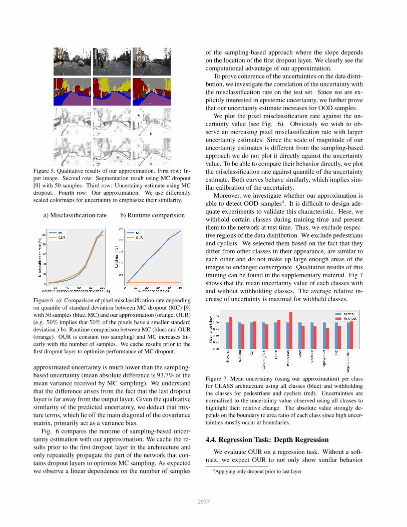
Figure 5. Qualitative results of our approximation. First row: In-

put image. Second row: Segmentation result using MC dropout

[9] with 50 samples. Third row: Uncertainty estimate using MC

dropout. Fourth row: Our approximation. We use differently

scaled colormaps for uncertainty to emphasize their similarity.

a) Misclassification rate b) Runtime comparision

Figure 6. a): Comparison of pixel misclassification rate depending

on quantile of standard deviation between MC dropout (MC) [9]

with 50 samples (blue, MC) and our approximation (orange, OUR)

(e.g. 50% implies that 50% of the pixels have a smaller standard

deviation.) b): Runtime comparison between MC (blue) and OUR

(orange). OUR is constant (no sampling) and MC increases lin-

early with the number of samples. We cache results prior to the

first dropout layer to optimize performance of MC dropout.

approximated uncertainty is much lower than the sampling-

based uncertainty (mean absolute difference is 93.7% of the

mean variance received by MC sampling). We understand

that the difference arises from the fact that the last dropout

layer is far away from the output layer. Given the qualitative

similarity of the predicted uncertainty, we deduct that mix-

ture terms, which lie off the main diagonal of the covariance

matrix, primarily act as a variance bias.

Fig. 6 compares the runtime of sampling-based uncer-

tainty estimation with our approximation. We cache the re-

sults prior to the first dropout layer in the architecture and

only repeatedly propagate the part of the network that con-

tains dropout layers to optimize MC sampling. As expected

we observe a linear dependence on the number of samples

of the sampling-based approach where the slope depends

on the location of the first dropout layer. We clearly see the

computational advantage of our approximation.

To prove coherence of the uncertainties on the data distri-

bution, we investigate the correlation of the uncertainty with

the misclassification rate on the test set. Since we are ex-

plicitly interested in epistemic uncertainty, we further prove

that our uncertainty estimate increases for OOD samples.

We plot the pixel misclassification rate against the un-

certainty value (see Fig. 6). Obviously we wish to ob-

serve an increasing pixel misclassification rate with larger

uncertainty estimates. Since the scale of magnitude of our

uncertainty estimates is different from the sampling-based

approach we do not plot it directly against the uncertainty

value. To be able to compare their behavior directly, we plot

the misclassification rate against quantile of the uncertainty

estimate. Both curves behave similarly, which implies sim-

ilar calibration of the uncertainty.

Moreover, we investigate whether our approximation is

able to detect OOD samples4. It is difficult to design ade-

quate experiments to validate this characteristic. Here, we

withhold certain classes during training time and present

them to the network at test time. Thus, we exclude respec-

tive regions of the data distribution. We exclude pedestrians

and cyclists. We selected them based on the fact that they

differ from other classes in their appearance, are similar to

each other and do not make up large enough areas of the

images to endanger convergence. Qualitative results of this

training can be found in the supplementary material. Fig 7

shows that the mean uncertainty value of each classes with

and without withholding classes. The average relative in-

crease of uncertainty is maximal for withheld classes.

Figure 7. Mean uncertainty (using our approximation) per class

for CLASS architecture using all classes (blue) and withholding

the classes for pedestrians and cyclists (red). Uncertainties are

normalized to the uncertainty value observed using all classes to

highlight their relative change. The absolute value strongly de-

pends on the boundary to area ratio of each class since high uncer-

tainties mostly occur at boundaries.

4.4. Regression Task: Depth Regression

We evaluate OUR on a regression task. Without a soft-

max, we expect OUR to not only show similar behavior

4Applying only dropout prior to last layer

2937

but also to be compellingly close to the sampling-based ap-

proach. We apply OUR to monocular depth regression [12].

The final activation of this architecture is a sigmoid func-

tion. Thus it is expected that OUR will not exaclty match

the sampling-based result. Following the original work,

we train on the KITTI dataset [11] and keep the setup un-

changed with exception of inserting a dropout layer prior

to the final convolution to estimate uncertainty. As uncer-

tainty estimate we choose the variance of the regression out-

put and we use Eq. 8, 9 and 10 to propagate variance. Note

that this setup does not require modeling the full covariance

matrix because sigmoid is an element-wise operation.

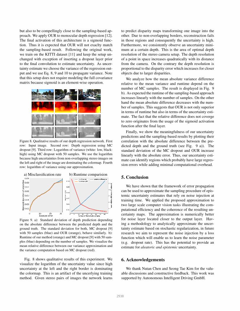
Figure 8. Qualitative results of our depth regression network. First

row: Input image. Second row: Depth regression using MC

dropout [9]. Third row: Logarithm of variance (white: low, black:

high) using MC dropout with 50 samples. We use the logarithm

because high uncertainties from non-overlapping stereo images on

the left and right of the image are dominating the colormap. Fourth

row: logarithm of variance using our approximation.

a) Misclassification rate b) Runtime comparision

Figure 9. a): Standard deviation of depth prediction depending

on the absolute difference between the predicted depth and the

ground truth. The standard deviation for both, MC dropout [9]

with 50 samples (blue) and OUR (orange), behave similarly. b):

Runtime of our method (orange) and MC dropout [9] with 50 sam-

ples (blue) depending on the number of samples. We visualize the

mean relative difference between our variance approximation and

the variance computation based on MC dropout (red).

Fig. 8 shows qualitative results of this experiment. We

visualize the logarithm of the uncertainty value since high

uncertainty at the left and the right border is dominating

the colormap. This is an artifact of the uncerlying training

method. Given stereo pairs of images the network learns

to predict disparity maps transforming one image into the

other. Due to non-overlapping borders, reconstruction fails

in those regions and consequently the uncertainty is high.

Furthermore, we consistently observe an uncertainty mini-

mum at a certain depth. This is the area of optimal depth

resolution of the stereo camera setup. The depth resolution

of a point in space increases quadratically with its distance

from the camera. On the contrary the depth resolution is

proportional to the disparity error which increases for closer

objects due to larger disparities.

We analyze how the mean absolute variance difference

relative to the mean variance and runtime depend on the

number of MC samples. The result is displayed in Fig. 9

b). As expected the runtime of the sampling-based approach

increases linearly with the number of samples. On the other

hand the mean absolute difference decreases with the num-

ber of samples. This suggests that OUR is not only superior

in terms of runtime but also in terms of the uncertainty esti-

mate. The fact that the relative difference does not coverge

to zero originates from the usage of the sigmoid activation

function after the final layer.

Finally, we show the meaningfulness of our uncertainty

predictions and the sampling-based results by plotting their

correlation with the absolute difference between the pre-

dicted depth and the ground truth (see Fig. 9 a)). The

standard deviation of the MC dropout and OUR increase

linearly with the absolute error. Thus, our uncertainty esti-

mate can identify regions which probably have large regres-

sion errors while adding minimal computational overhead.

5. Conclusion

We have shown that the framework of error propagation

can be used to approximate the sampling procedure of epis-

temic uncertainty estimates that rely on noise injection at

training time. We applied the proposed approximation to

two large scale computer vision tasks illustrating the com-

putational efficiency and the coherence of the resulting un-

certainty maps. The approximation is numerically better

for noise layer located closer to the output layer. Hav-

ing a methodology to analytically approximate the uncer-

tainty estimate based on stochastic regularization, in future

research we aim to represent the noise injection by a loss

function which will enable us to learn the noise parameter

(e.g. dropout rate). This has the potential to provide an

estimate for aleatoric and epistemic uncertainty.

6. Acknowledgements

We thank Nutan Chen and Seong Tae Kim for the valu-

able discussions and constructive feedback. This work was

supported by Autonomous Intelligent Driving GmbH.

2938

References

[1] Apratim Bhattacharyya, Mario Fritz, and Bernt Schiele.

Long-term on-board prediction of people in traffic scenes

under uncertainty. In Proceedings of the IEEE Conference

on Computer Vision and Pattern Recognition, pages 4194–

4202, 2018.

[2] Christopher M Bishop. Mixture density networks. Technical

report, Citeseer, 1994.

[3] Charles Blundell, Julien Cornebise, Koray Kavukcuoglu,

and Daan Wierstra. Weight uncertainty in neural network.

In International Conference on Machine Learning, pages

1613–1622, 2015.

[4] Gabriel J Brostow, Julien Fauqueur, and Roberto Cipolla.

Semantic object classes in video: A high-definition ground

truth database. Pattern Recognition Letters, 30(2):88–97,

2009.

[5] Sungjoon Choi, Kyungjae Lee, Sungbin Lim, and Songhwai

Oh. Uncertainty-aware learning from demonstration using

mixture density networks with sampling-free variance mod-

eling. In 2018 IEEE International Conference on Robotics

and Automation (ICRA), pages 6915–6922. IEEE, 2018.

[6] Bradley Efron and Robert J Tibshirani. An introduction to

the bootstrap. CRC press, 1994.

[7] Di Feng, Lars Rosenbaum, and Klaus Dietmayer. Towards

safe autonomous driving: Capture uncertainty in the deep

neural network for lidar 3d vehicle detection. In 2018 21st

International Conference on Intelligent Transportation Sys-

tems (ITSC), pages 3266–3273. IEEE, 2018.

[8] Yarin Gal. Uncertainty in deep learning. PhD thesis, PhD

thesis, University of Cambridge, 2016.

[9] Yarin Gal and Zoubin Ghahramani. Dropout as a bayesian

approximation: Representing model uncertainty in deep

learning. In international conference on machine learning,

pages 1050–1059, 2016.

[10] Yarin Gal, Riashat Islam, and Zoubin Ghahramani. Deep

bayesian active learning with image data. In Proceedings

of the 34th International Conference on Machine Learning-

Volume 70, pages 1183–1192. JMLR. org, 2017.

[11] Andreas Geiger, Philip Lenz, Christoph Stiller, and Raquel

Urtasun. Vision meets robotics: The kitti dataset. The Inter-

national Journal of Robotics Research, 32(11):1231–1237,

2013.

[12] Clement Godard, Oisin Mac Aodha, and Gabriel J Bros-

tow. Unsupervised monocular depth estimation with left-

right consistency. In Proceedings of the IEEE Conference on

Computer Vision and Pattern Recognition, pages 270–279,

2017.

[13] Leo A Goodman. On the exact variance of products. Journal

of the American statistical association, 55(292):708–713,

1960.

[14] Jose Miguel Hernandez-Lobato and Ryan Adams. Prob-

abilistic backpropagation for scalable learning of bayesian

neural networks. In International Conference on Machine

Learning, pages 1861–1869, 2015.

[15] Po-Yu Huang, Wan-Ting Hsu, Chun-Yueh Chiu, Ting-Fan

Wu, and Min Sun. Efficient uncertainty estimation for se-

mantic segmentation in videos. In Proceedings of the Euro-

pean Conference on Computer Vision (ECCV), pages 520–

535, 2018.

[16] Seong Jae Hwang, Ronak Mehta, and Vikas Singh.

Sampling-free uncertainty estimation in gated recurrent units

with exponential families. arXiv preprint arXiv:1804.07351,

2018.

[17] Michael Kampffmeyer, Arnt-Borre Salberg, and Robert

Jenssen. Semantic segmentation of small objects and mod-

eling of uncertainty in urban remote sensing images using

deep convolutional neural networks. In Proceedings of the

IEEE conference on computer vision and pattern recognition

workshops, pages 1–9, 2016.

[18] Alex Kendall, Vijay Badrinarayanan, and Roberto Cipolla.

Bayesian segnet: Model uncertainty in deep convolu-

tional encoder-decoder architectures for scene understand-

ing. CoRR, abs/1511.02680, 2015.

[19] Alex Kendall and Yarin Gal. What uncertainties do we need

in bayesian deep learning for computer vision? In Advances

in neural information processing systems, pages 5574–5584,

2017.

[20] Balaji Lakshminarayanan, Alexander Pritzel, and Charles

Blundell. Simple and scalable predictive uncertainty esti-

mation using deep ensembles. In Advances in Neural Infor-

mation Processing Systems, pages 6402–6413, 2017.

[21] Michael Truong Le, Frederik Diehl, Thomas Brunner, and

Alois Knol. Uncertainty estimation for deep neural object

detectors in safety-critical applications. In 2018 21st Inter-

national Conference on Intelligent Transportation Systems

(ITSC), pages 3873–3878. IEEE, 2018.

[22] Marcin Mozejko, Mateusz Susik, and Rafał Karczewski.

Inhibited softmax for uncertainty estimation in neural net-

works. arXiv preprint arXiv:1810.01861, 2018.

[23] Ian Osband, Charles Blundell, Alexander Pritzel, and Ben-

jamin Van Roy. Deep exploration via bootstrapped dqn. In

Advances in neural information processing systems, pages

4026–4034, 2016.

[24] Christian Rupprecht, Iro Laina, Robert DiPietro, Maximil-

ian Baust, Federico Tombari, Nassir Navab, and Gregory D

Hager. Learning in an uncertain world: Representing am-

biguity through multiple hypotheses. In Proceedings of the

IEEE International Conference on Computer Vision, pages

3591–3600, 2017.

[25] Jasper Snoek, Hugo Larochelle, and Ryan P Adams. Prac-

tical bayesian optimization of machine learning algorithms.

In Advances in neural information processing systems, pages

2951–2959, 2012.

[26] John Taylor. Introduction to error analysis, the study of un-

certainties in physical measurements. 1997.

[27] Mattias Teye, Hossein Azizpour, and Kevin Smith. Bayesian

uncertainty estimation for batch normalized deep networks.

In International Conference on Machine Learning, pages

4914–4923, 2018.

[28] Hao Wang, SHI Xingjian, and Dit-Yan Yeung. Natural-

parameter networks: A class of probabilistic neural net-

works. In Advances in Neural Information Processing Sys-

tems, pages 118–126, 2016.

2939

[29] Sida Wang and Christopher Manning. Fast dropout training.

In international conference on machine learning, pages 118–

126, 2013.

[30] Anqi Wu, Sebastian Nowozin, Edward Meeds, Richard E

Turner, Jose Miguel Hernandez-Lobato, and Alexander L

Gaunt. Deterministic variational inference for robust

bayesian neural networks. 2018.

[31] Guodong Zhang, Shengyang Sun, David Duvenaud, and

Roger Grosse. Noisy natural gradient as variational infer-

ence. In International Conference on Machine Learning,

pages 5847–5856, 2018.

2940