Supplementary MaterialDetails of the Model

Both DCP-v1 and DCP-v2 use DGCNN to embed pointclouds. In DGCNN, we use five EdgeConv layers. The num-bers of filters per layer are [64, 64, 128, 256, 512]. In eachEdgeConv layer, BatchNorm is used [2] with 0.1 momentum,followed by ReLU [4]. Following [9], we concatenate theoutputs from the first four layers and feed them into the lastone. Our local aggregation function is max, and no globalaggregation function is needed.

For DCP-v2, in the Transformer layer, the architecture isthe same as the one proposed in [8]. The only difference isthat we do not add positional encoding, because the positionof each point in R3 is not correlated with its index in thearray.

We use one encoder and one decoder. In both the encoderand decoder, we use multi-head attention with 4 heads and512 embedding dimensions, followed by a MLP with 1024hidden dimensions. ReLU [4] is also used in the MLP. Insidethe Transformer, LayerNorm [1] is used after MLP and multi-head attention and before the residual connection. Unlike[8], we do not use Dropout [7].

We use PyTorch’s [5] built-in SVD layer. Other numericalsolvers that support gradient backpropagation could also beused to recover the rigid transformation.

Adam [3] with initial learning rate 0.001 is used for train-ing. The coefficients used for computing running averagesof the gradient and its square are 0.9 and 0.999, resp.

We use weight decay 10−4 to regularize the model. Wetrain the model a total of 250 epochs, and at epochs 75, 150and 200, the learning rate is divided by 10.

The MLP we use in ablation study has 3 fully connectedlayers and the number of filters are [256, 128, 64] respec-tively. BatchNorm [3] and ReLU [4] are used after eachfully connected layer. Finally, another two fully connectedlayers are used to project the embeddings to quaternion andtranslation vector separately.

The architecture of PointNet in ablation study is the sameas the basic version in [6]. The number of filters in eachlayer are [64, 64, 64, 128, 512].

Additional Figures

We provide additional figures of results with DCP-v2tested on different objects in Figure 1. Figure 2 shows resultsin which we test with rotations in all of SE(3), meaningalong each axis, we randomly sample rotations in [0, 360◦].The model used here is still trained with rotations in [0, 45◦].As shown in Figure 2, our model generalizes reasonablywell to large motions. Figure 3 shows the results of DCP-v2 tested on noisy point clouds. The noise (sampled fromN (0, 0.01)) is added independently to each point of twoinput point clouds.

Model MSE(R) RMSE(R) MAE(R) MSE(t) RMSE(t) MAE(t)

ICP 2845.295 53.341 45.415 0.084 0.289 0.248Go-ICP 3778.314 61.468 35.032 0.004 0.066 0.033FGR 560.506 23.675 8.118 0.001 0.029 0.007PointNetLK 4826.940 69.476 44.307 0.006 0.080 0.047

DCP-v2 (ours) 225.736 15.025 2.260 0.000002 0.001 0.001

Table 1. ModelNet40: Test on unseen point clouds ([0, 90◦])

Model MSE(R) RMSE(R) MAE(R) MSE(t) RMSE(t) MAE(t)

ICP 11175.784 105.716 90.713 0.085 0.292 0.250Go-ICP 13169.908 114.760 92.941 0.013 0.115 0.080FGR 13808.102 117.508 87.678 0.008 0.090 0.047PointNetLK 13751.237 117.266 94.539 0.011 0.104 0.067

DCP-v2 (ours) 13152.160 114.683 78.333 0.000005 0.002 0.001

Table 2. ModelNet40: Test on unseen point clouds ([0, 180◦])

Model MSE(R) RMSE(R) MAE(R) MSE(t) RMSE(t) MAE(t)

ICP 1125.095 33.542 25.032 0.088 0.296 0.251Go-ICP 216.790 14.724 3.511 0.001 0.032 0.012FGR 130.621 11.429 2.960 0.001 0.032 0.008PointNetLK 374.948 19.364 7.389 0.003 0.053 0.029

DCP-v2 (ours) 23.471 4.845 2.486 0.001 0.033 0.024

Table 3. ModelNet40: Test on unseen partial point clouds ([0, 45◦])

# Iters MSE(R) RMSE(R) MAE(R) MSE(t) RMSE(t) MAE(t)

1 1.307329 1.143385 0.770573 0.000003 0.001786 0.0011953 0.568834 0.754211 0.223045 0.000001 0.000872 0.0005195 0.267259 0.516971 0.168858 0.000001 0.000870 0.0005187 0.163877 0.404817 0.145387 0.000001 0.000870 0.000517

Table 4. ModelNet40: Test on unseen point clouds (iterative infer-ence on testing, [0, 45◦])

Additional Ablation Studies

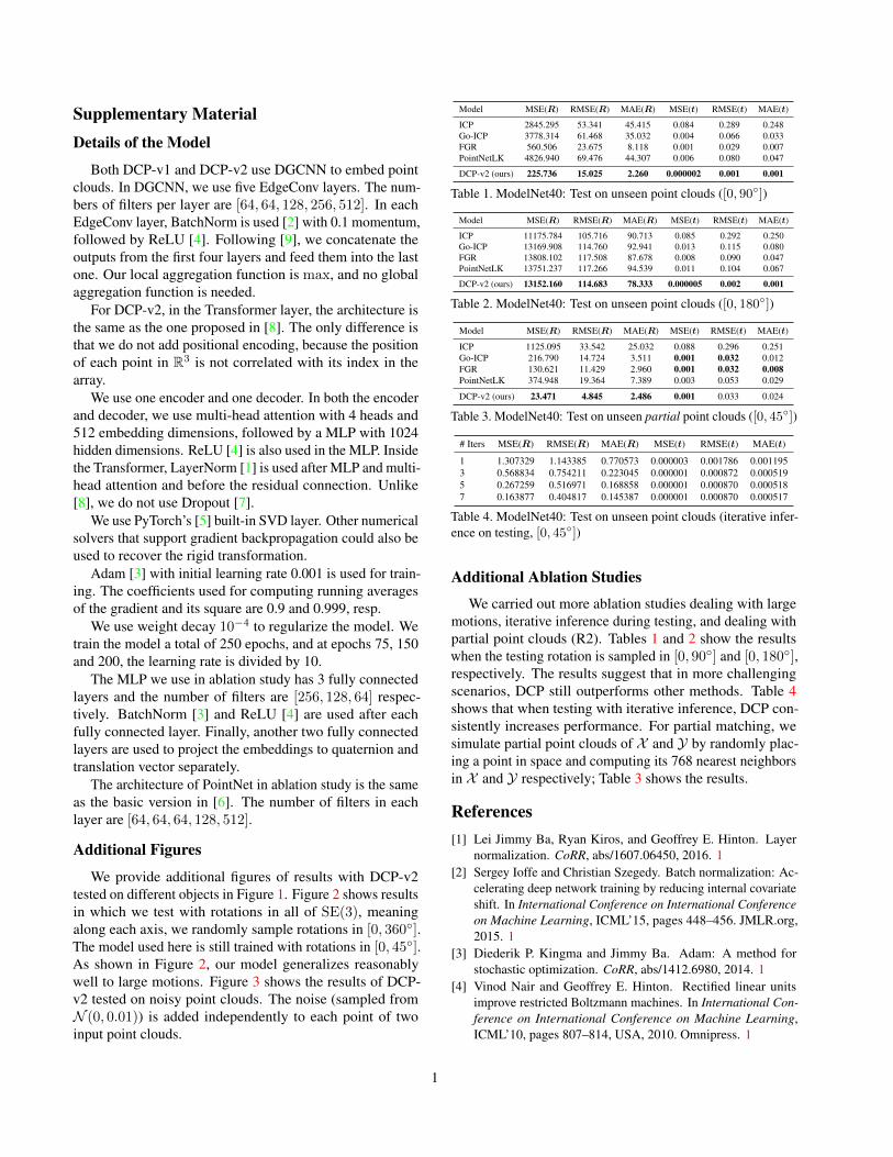
We carried out more ablation studies dealing with largemotions, iterative inference during testing, and dealing withpartial point clouds (R2). Tables 1 and 2 show the resultswhen the testing rotation is sampled in [0, 90◦] and [0, 180◦],respectively. The results suggest that in more challengingscenarios, DCP still outperforms other methods. Table 4shows that when testing with iterative inference, DCP con-sistently increases performance. For partial matching, wesimulate partial point clouds of X and Y by randomly plac-ing a point in space and computing its 768 nearest neighborsin X and Y respectively; Table 3 shows the results.

References[1] Lei Jimmy Ba, Ryan Kiros, and Geoffrey E. Hinton. Layer

normalization. CoRR, abs/1607.06450, 2016. 1[2] Sergey Ioffe and Christian Szegedy. Batch normalization: Ac-

celerating deep network training by reducing internal covariateshift. In International Conference on International Conferenceon Machine Learning, ICML’15, pages 448–456. JMLR.org,2015. 1

[3] Diederik P. Kingma and Jimmy Ba. Adam: A method forstochastic optimization. CoRR, abs/1412.6980, 2014. 1

[4] Vinod Nair and Geoffrey E. Hinton. Rectified linear unitsimprove restricted Boltzmann machines. In International Con-ference on International Conference on Machine Learning,ICML’10, pages 807–814, USA, 2010. Omnipress. 1

1

Input

Output

Input

Output

Input

Output

Figure 1. Results of DCP-v2. Top: inputs. Bottom: outputs of DCP-v2.

[5] Adam Paszke, Sam Gross, Soumith Chintala, Gregory Chanan,Edward Yang, Zachary DeVito, Zeming Lin, Alban Desmaison,Luca Antiga, and Adam Lerer. Automatic differentiation inPyTorch. 2017. 1

[6] Charles Ruizhongtai Qi, Hao Su, Kaichun Mo, and Leonidas J.Guibas. PointNet: Deep learning on point sets for 3D classi-fication and segmentation. In IEEE Conference on ComputerVision and Pattern Recognition (CVPR), pages 77–85. IEEEComputer Society, 2017. 1

[7] Nitish Srivastava, Geoffrey Hinton, Alex Krizhevsky, IlyaSutskever, and Ruslan Salakhutdinov. Dropout: A simple wayto prevent neural networks from overfitting. J. Mach. Learn.Res., 15(1):1929–1958, Jan. 2014. 1

[8] Ashish Vaswani, Noam Shazeer, Niki Parmar, Jakob Uszkoreit,Llion Jones, Aidan N Gomez, Łukasz Kaiser, and Illia Polo-sukhin. Attention is all you need. In I. Guyon, U. V. Luxburg,S. Bengio, H. Wallach, R. Fergus, S. Vishwanathan, and R.Garnett, editors, Advances in Neural Information ProcessingSystems 30, pages 5998–6008. Curran Associates, Inc., 2017.1

[9] Yue Wang, Yongbin Sun, Sanjay E. Sarma Ziwei Liu,Michael M. Bronstein, and Justin M. Solomon. Dynamic

graph CNN for learning on point clouds. ACM Transactionson Graphics, to appear, 2019. 1

2

Input

Output

Figure 2. Results of DCP-v2 tested with large motion. Top: inputs. Down: outputs of DCP-v2

3

Input

Output

Input

Output

Figure 3. Results of DCP-v2 tested on noisy point clouds. Top: inputs. Down: outputs of DCP-v2

4