Graduate Macroeconomics 2Lecture 1 - Introduction to Real Business Cycles

Zsofia L. Barany

Sciences Po

2014 January

About the course I.

I 2-hour lecture every week, Tuesdays from 10:15-12:15I 2 big topics covered:

1. economic fluctuations2. unemployment

I office hour by appointment, in office E.404

I email: zsofia.barany@sciencespo.fr

I lecture notes will become available weekly before the lecture

About the course II.

I besides the lectures, there will be classes every Mondayafternoon

I tutorials in 3 groups

I for most of the classes you will have to solve problem sets

I you will have to hand in 2 problem sets, these will constitute30 percent of your final grade

I you will receive the solution to the problem sets

Let’s start!

Why study business cycles?

I last term you studied long-run growth→ clearly a very important determinant of welfare

I now we will look at short-term fluctuationsI why do we care about these?

I fluctuations are unpleasantI especially increases in unemployment and inflation

I ⇒ governments tend to want to dampen these cycles

I we need to understand the driving forces behind thefluctuations of the economy

A very-very brief history 1.the Great Depression and Keynes

I Keynes: short-run rigidity of wages (and prices) ⇒ stableequilibrium with unemployment possibleaggregate demand is the key ⇒ government intervention

I others formalized his ideas:

I → the IS (investment and saving) – LM (money demand andsupply) modellater addition: Phillips curve - tradeoff between inflation andunemployment

I → similar much bigger models with several hundred equations

I these models are based on empirically observed relationshipsbetween: output and consumption, money demand, inflation,unemployment, etc

I the aim of these models was to predict the effects of policies

I they were pretty successful at it until the 1960s

A very-very brief history 2.

the Neo Classicals

I monetarism - FriedmanI permanent income hypothesis → small fiscal policy multipliersI bad monetary policy causes economic fluctuations (not ”animal

spirits”) → prescription: steady growth in monetary aggregatesI Phillips curve relationship does not hold in the long run ↔

money is neutralit appears in the short run due to unanticipated inflation andmoney illusion

I the rational expectations revolution - LucasI Keynesian empirical relationships estimated given a policy

for an alternative policy the relationship would be different dueto changes in expectations→ Keynesian models not suitable for policy evaluation

I monetary policy only matters if it surprises peopleI → systematic monetary policy aimed at stabilizing the

economy will not work

A very-very brief history 3.

the Neo Classical Real Business Cycle Theory

I prices adjust instantaneously to clear markets

I economic actors optimize, and are forward looking

I rational expectations

I cause of fluctuations: random shocks to technology

I key mechanism: intertemporal substitution in consumptionand leisure as a response to these shocks

today:

I methodological contribution is most emphasized

I important to assess how close reality is to a perfectly working,frictionless environment→ to understand the importance of market imperfections

A very-very brief history 4.the New Keynesians

I general disequilibriumI tools of general equilibrium to analyze the allocations of

resources when markets do not clearI how does the not clearing of one market influence supply and

demand in another marketI fixed prices and wagesI → different regimes can arise, i.e. ”Keynesian regime” excess

supply in goods and labor

I rational expectations without market clearingI systematic mon policy can stabilize the economy

I why don’t wages and prices clear the markets?I menu costsI efficiency wagesI wage and price setters aren’t perfectly rationalI market power → wedge between privately and socially optimal

price adjustment

Dynamic Stochastic General Equilibrium (DSGE) models

D some things don’t make sense in static models (forexample: investment)relatively short-term analysis

S shocks hit the economy, and force it off the balancedgrowth path (BGP) ⇒fluctuations do not mean dis-equilibrium, this is thereaction of the economy to an outside shock

G E this is macroI the models are based on

I perfectly/monopolistically competitive marketsI optimizing agents

⇒ the economy is in EQUILIBRIUMI micro-founded models

There are different schools of thought...

SUBSTANTIVE DIFFERENCES

ME

TH

OD

OL

OG

ICA

LD

IFF

ER

EN

CE

Ssupply demand shocksshocks rigidity

simple SALT WATER → aim:models/ A · LαK 1−α contributed what see thequalitative growth model is important mechanismsinsights RIGIDITY very clearly

complex FRESH WATER now there is →models contributed more harmony transparencyquantitative the in macro is the costmatching METHODOLOGY

↓we are goingto start here,because it is

easier

Path to get there:

1. real business cycle (RBC) models

2. introduce market power - New Keynesian (NK) model 1.

3. introduce money

4. introduce nominal rigidities - NK model 2.

The predictions in the end are not very different from the IS-LM.

However, better sense

I of the role of distortions

I of optimal policy

Business Cycle Facts I.

properties of quarterly detrended macro time series

xt = log(Xt)− log(X ∗t )

is the percentage deviation of variable X from its trend, X ∗

how is the trend defined? (you have seen this in class yesterday)

I first linear

I now more sophisticated bandpass filter

→ growth theory serves as a guidance

Business Cycle Facts II.

look at the highest correlation with GDP

ρ(xt , yt+k) k = −6,−5, ..., 0, ...5, 6

I if ρ > 0, then x is pro-cyclical

I if ρ < 0, then x is counter-cyclical

I if k < 0, then x lags behind output

I if k > 0, then x leads output

Business Cycle Facts III.

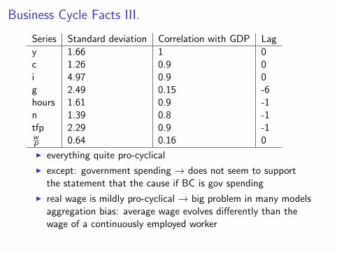
Series Standard deviation Correlation with GDP Lag

y 1.66 1 0c 1.26 0.9 0i 4.97 0.9 0g 2.49 0.15 -6hours 1.61 0.9 -1n 1.39 0.8 -1tfp 2.29 0.9 -1wP 0.64 0.16 0

I everything quite pro-cyclical

I except: government spending → does not seem to supportthe statement that the cause if BC is gov spending

I real wage is mildly pro-cyclical → big problem in many modelsaggregation bias: average wage evolves differently than thewage of a continuously employed worker

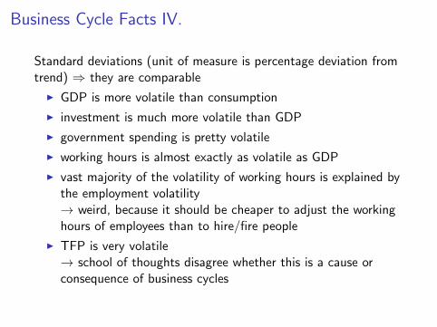
Business Cycle Facts IV.

Standard deviations (unit of measure is percentage deviation fromtrend) ⇒ they are comparable

I GDP is more volatile than consumption

I investment is much more volatile than GDP

I government spending is pretty volatile

I working hours is almost exactly as volatile as GDP

I vast majority of the volatility of working hours is explained bythe employment volatility→ weird, because it should be cheaper to adjust the workinghours of employees than to hire/fire people

I TFP is very volatile→ school of thoughts disagree whether this is a cause orconsequence of business cycles

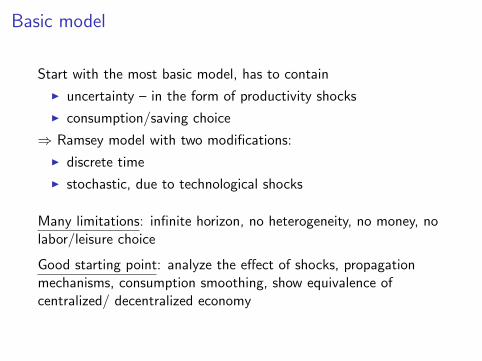
Basic model

Start with the most basic model, has to contain

I uncertainty – in the form of productivity shocks

I consumption/saving choice

⇒ Ramsey model with two modifications:

I discrete time

I stochastic, due to technological shocks

Many limitations: infinite horizon, no heterogeneity, no money, nolabor/leisure choice

Good starting point: analyze the effect of shocks, propagationmechanisms, consumption smoothing, show equivalence ofcentralized/ decentralized economy

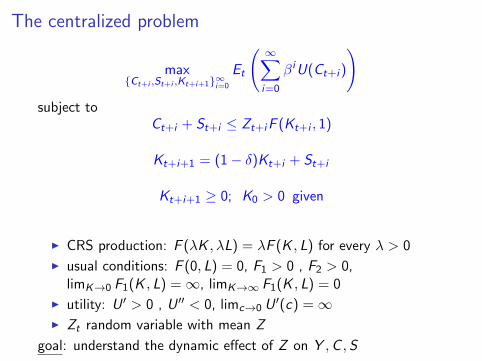
The centralized problem

max{Ct+i ,St+i ,Kt+i+1}∞i=0

Et

( ∞∑i=0

βiU(Ct+i )

)subject to

Ct+i + St+i ≤ Zt+iF (Kt+i , 1)

Kt+i+1 = (1− δ)Kt+i + St+i

Kt+i+1 ≥ 0; K0 > 0 given

I CRS production: F (λK , λL) = λF (K , L) for every λ > 0

I usual conditions: F (0, L) = 0, F1 > 0 , F2 > 0,limK→0 F1(K , L) =∞, limK→∞ F1(K , L) = 0

I utility: U ′ > 0 , U ′′ < 0, limc→0 U′(c) =∞

I Zt random variable with mean Z

goal: understand the dynamic effect of Z on Y ,C ,S

The first order conditions

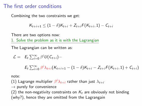
Combining the two constraints we get:

Kt+i+1 ≤ (1− δ)Kt+i + Zt+iF (Kt+i , 1)− Ct+i

There are two options now:1. Solve the problem as it is with the Lagrangian

The Lagrangian can be written as:

L = Et∑∞

i=0 βiU(Ct+i )−

Et∑∞

i=0 βiλt+i (Kt+i+1 − (1− δ)Kt+i − Zt+iF (Kt+i , 1) + Ct+i )

note:(1) Lagrange multiplier βiλt+i rather than just λt+i

→ purely for convenience(2) the non-negativity constraints on Kt are obviously not binding(why?), hence they are omitted from the Lagrangain

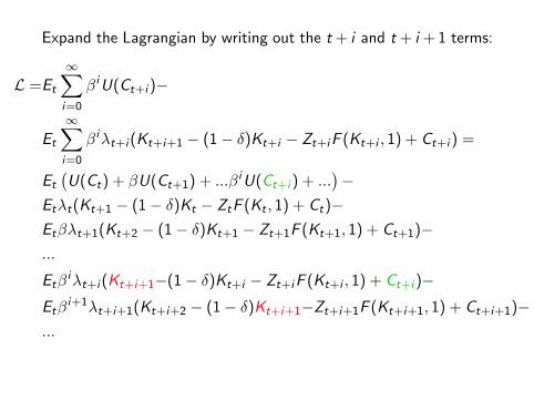
Expand the Lagrangian by writing out the t + i and t + i + 1 terms:

L =Et

∞∑i=0

βiU(Ct+i )−

Et

∞∑i=0

βiλt+i (Kt+i+1 − (1− δ)Kt+i − Zt+iF (Kt+i , 1) + Ct+i ) =

Et

(U(Ct) + βU(Ct+1) + ...βiU(Ct+i ) + ...

)−

Etλt(Kt+1 − (1− δ)Kt − ZtF (Kt , 1) + Ct)−Etβλt+1(Kt+2 − (1− δ)Kt+1 − Zt+1F (Kt+1, 1) + Ct+1)−...

Etβiλt+i (Kt+i+1−(1− δ)Kt+i − Zt+iF (Kt+i , 1) + Ct+i )−

Etβi+1λt+i+1(Kt+i+2 − (1− δ)Kt+i+1−Zt+i+1F (Kt+i+1, 1) + Ct+i+1)−

...

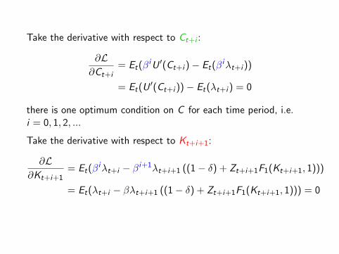
Take the derivative with respect to Ct+i :

∂L∂Ct+i

= Et(βiU ′(Ct+i )− Et(β

iλt+i ))

= Et(U′(Ct+i ))− Et(λt+i ) = 0

there is one optimum condition on C for each time period, i.e.i = 0, 1, 2, ...

Take the derivative with respect to Kt+i+1:

∂L∂Kt+i+1

= Et(βiλt+i − βi+1λt+i+1 ((1− δ) + Zt+i+1F1(Kt+i+1, 1)))

= Et(λt+i − βλt+i+1 ((1− δ) + Zt+i+1F1(Kt+i+1, 1))) = 0

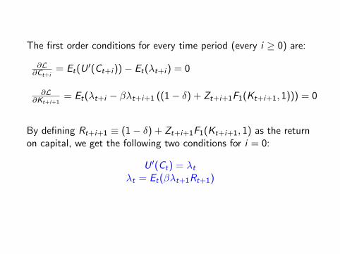
The first order conditions for every time period (every i ≥ 0) are:

∂L∂Ct+i

= Et(U′(Ct+i ))− Et(λt+i ) = 0

∂L∂Kt+i+1

= Et(λt+i − βλt+i+1 ((1− δ) + Zt+i+1F1(Kt+i+1, 1))) = 0

By defining Rt+i+1 ≡ (1− δ) + Zt+i+1F1(Kt+i+1, 1) as the returnon capital, we get the following two conditions for i = 0:

U ′(Ct) = λtλt = Et(βλt+1Rt+1)

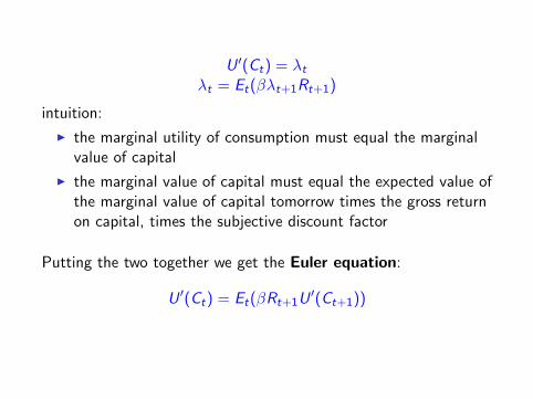
U ′(Ct) = λtλt = Et(βλt+1Rt+1)

intuition:

I the marginal utility of consumption must equal the marginalvalue of capital

I the marginal value of capital must equal the expected value ofthe marginal value of capital tomorrow times the gross returnon capital, times the subjective discount factor

Putting the two together we get the Euler equation:

U ′(Ct) = Et(βRt+1U′(Ct+1))

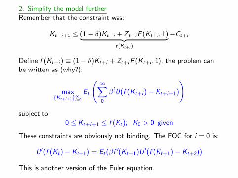
2. Simplify the model furtherRemember that the constraint was:

Kt+i+1 ≤ (1− δ)Kt+i + Zt+iF (Kt+i , 1)︸ ︷︷ ︸f (Kt+i )

−Ct+i

Define f (Kt+i ) ≡ (1− δ)Kt+i + Zt+iF (Kt+i , 1), the problem canbe written as (why?):

max{Kt+i+1}∞i=0

Et

( ∞∑0

βiU(f (Kt+i )− Kt+i+1)

)

subject to0 ≤ Kt+i+1 ≤ f (Kt); K0 > 0 given

These constraints are obviously not binding. The FOC for i = 0 is:

U ′(f (Kt)− Kt+1) = Et(βf′(Kt+1)U ′(f (Kt+1)− Kt+2))

This is another version of the Euler equation.

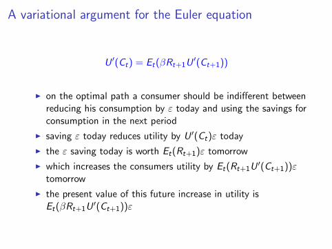
A variational argument for the Euler equation

U ′(Ct) = Et(βRt+1U′(Ct+1))

I on the optimal path a consumer should be indifferent betweenreducing his consumption by ε today and using the savings forconsumption in the next period

I saving ε today reduces utility by U ′(Ct)ε today

I the ε saving today is worth Et(Rt+1)ε tomorrow

I which increases the consumers utility by Et(Rt+1U′(Ct+1))ε

tomorrow

I the present value of this future increase in utility isEt(βRt+1U

′(Ct+1))ε

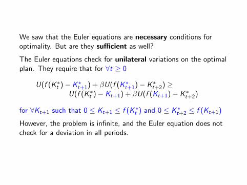
We saw that the Euler equations are necessary conditions foroptimality. But are they sufficient as well?

The Euler equations check for unilateral variations on the optimalplan. They require that for ∀t ≥ 0

U(f (K ∗t )− K ∗t+1) + βU(f (K ∗t+1)− K ∗t+2) ≥U(f (K ∗t )− Kt+1) + βU(f (Kt+1)− K ∗t+2)

for ∀Kt+1 such that 0 ≤ Kt+1 ≤ f (K ∗t ) and 0 ≤ K ∗t+2 ≤ f (Kt+1)

However, the problem is infinite, and the Euler equation does notcheck for a deviation in all periods.

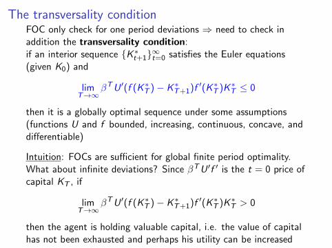
The transversality conditionFOC only check for one period deviations ⇒ need to check inaddition the transversality condition:if an interior sequence {K ∗t+1}∞t=0 satisfies the Euler equations(given K0) and

limT→∞

βTU ′(f (K ∗T )− K ∗T+1)f ′(K ∗T )K ∗T ≤ 0

then it is a globally optimal sequence under some assumptions(functions U and f bounded, increasing, continuous, concave, anddifferentiable)

Intuition: FOCs are sufficient for global finite period optimality.What about infinite deviations? Since βTU ′f ′ is the t = 0 price ofcapital KT , if

limT→∞

βTU ′(f (K ∗T )− K ∗T+1)f ′(K ∗T )K ∗T > 0

then the agent is holding valuable capital, i.e. the value of capitalhas not been exhausted and perhaps his utility can be increased

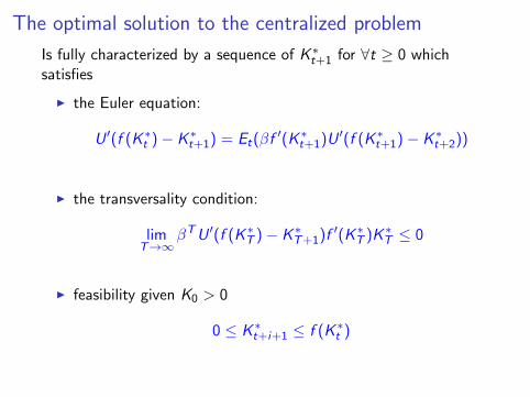
The optimal solution to the centralized problem

Is fully characterized by a sequence of K ∗t+1 for ∀t ≥ 0 whichsatisfies

I the Euler equation:

U ′(f (K ∗t )− K ∗t+1) = Et(βf′(K ∗t+1)U ′(f (K ∗t+1)− K ∗t+2))

I the transversality condition:

limT→∞

βTU ′(f (K ∗T )− K ∗T+1)f ′(K ∗T )K ∗T ≤ 0

I feasibility given K0 > 0

0 ≤ K ∗t+i+1 ≤ f (K ∗t )

The decentralized economy

To formulate the decentralized problem we have to decide

I whether firms rent or buy the capital

I how firms are financed (through retained earnings, bonds,equity)

Here I assume that the capital is owned by the consumers, whorent out the capital to firms.

main assumption: the goods, labor and capital markets areperfectly competitive

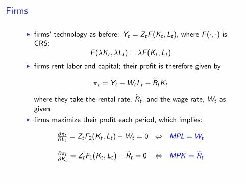
Firms

I firms’ technology as before: Yt = ZtF (Kt , Lt), where F (·, ·) isCRS:

F (λKt , λLt) = λF (Kt , Lt)

I firms rent labor and capital; their profit is therefore given by

πt = Yt −WtLt − RtKt

where they take the rental rate, Rt , and the wage rate, Wt asgiven

I firms maximize their profit each period, which implies:

∂πt∂Lt

= ZtF2(Kt , Lt)−Wt = 0 ⇔ MPL = Wt

∂πt∂Kt

= ZtF1(Kt , Lt)− Rt = 0 ⇔ MPK = Rt

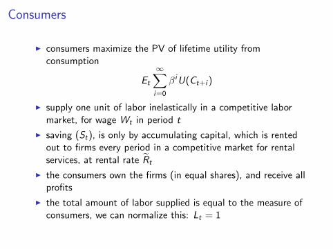
Consumers

I consumers maximize the PV of lifetime utility fromconsumption

Et

∞∑i=0

βiU(Ct+i )

I supply one unit of labor inelastically in a competitive labormarket, for wage Wt in period t

I saving (St), is only by accumulating capital, which is rentedout to firms every period in a competitive market for rentalservices, at rental rate Rt

I the consumers own the firms (in equal shares), and receive allprofits

I the total amount of labor supplied is equal to the measure ofconsumers, we can normalize this: Lt = 1

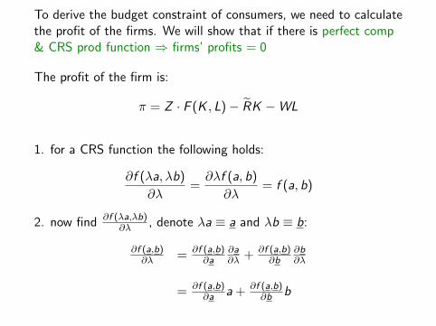
To derive the budget constraint of consumers, we need to calculatethe profit of the firms. We will show that if there is perfect comp& CRS prod function ⇒ firms’ profits = 0

The profit of the firm is:

π = Z · F (K , L)− RK −WL

1. for a CRS function the following holds:

∂f (λa, λb)

∂λ=∂λf (a, b)

∂λ= f (a, b)

2. now find ∂f (λa,λb)∂λ , denote λa ≡ a and λb ≡ b:

∂f (a,b)∂λ = ∂f (a,b)

∂a∂a∂λ + ∂f (a,b)

∂b∂b∂λ

= ∂f (a,b)∂a a + ∂f (a,b)

∂b b

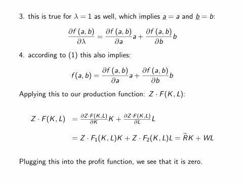
3. this is true for λ = 1 as well, which implies a = a and b = b:

∂f (a, b)

∂λ=∂f (a, b)

∂aa +

∂f (a, b)

∂bb

4. according to (1) this also implies:

f (a, b) =∂f (a, b)

∂aa +

∂f (a, b)

∂bb

Applying this to our production function: Z · F (K , L):

Z · F (K , L) = ∂Z ·F (K ,L)∂K K + ∂Z ·F (K ,L)

∂L L

= Z · F1(K , L)K + Z · F2(K , L)L = RK + WL

Plugging this into the profit function, we see that it is zero.

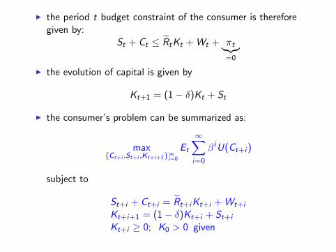
I the period t budget constraint of the consumer is thereforegiven by:

St + Ct ≤ RtKt + Wt + πt︸︷︷︸=0

I the evolution of capital is given by

Kt+1 = (1− δ)Kt + St

I the consumer’s problem can be summarized as:

max{Ct+i ,St+i ,Kt+i+1}∞i=0

Et

∞∑i=0

βiU(Ct+i )

subject to

St+i + Ct+i = Rt+iKt+i + Wt+i

Kt+i+1 = (1− δ)Kt+i + St+i

Kt+i ≥ 0; K0 > 0 given

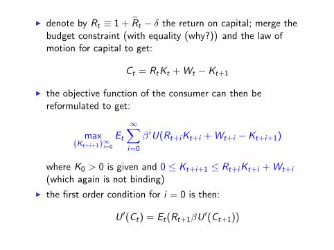
I denote by Rt ≡ 1 + Rt − δ the return on capital; merge thebudget constraint (with equality (why?)) and the law ofmotion for capital to get:

Ct = RtKt + Wt − Kt+1

I the objective function of the consumer can then bereformulated to get:

max{Kt+i+1}∞i=0

Et

∞∑i=0

βiU(Rt+iKt+i + Wt+i − Kt+i+1)

where K0 > 0 is given and 0 ≤ Kt+i+1 ≤ Rt+iKt+i + Wt+i

(which again is not binding)

I the first order condition for i = 0 is then:

U ′(Ct) = Et(Rt+1βU′(Ct+1))

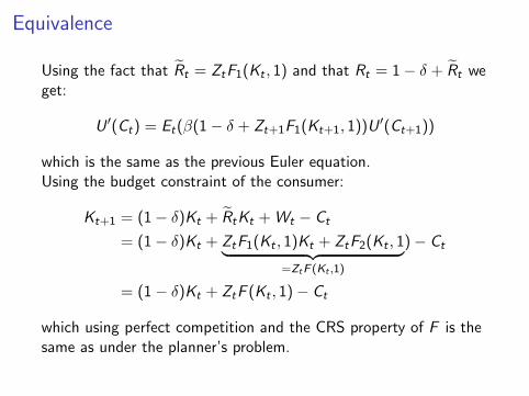
Equivalence

Using the fact that Rt = ZtF1(Kt , 1) and that Rt = 1− δ + Rt weget:

U ′(Ct) = Et(β(1− δ + Zt+1F1(Kt+1, 1))U ′(Ct+1))

which is the same as the previous Euler equation.Using the budget constraint of the consumer:

Kt+1 = (1− δ)Kt + RtKt + Wt − Ct

= (1− δ)Kt + ZtF1(Kt , 1)Kt + ZtF2(Kt , 1︸ ︷︷ ︸=ZtF (Kt ,1)

)− Ct

= (1− δ)Kt + ZtF (Kt , 1)− Ct

which using perfect competition and the CRS property of F is thesame as under the planner’s problem.

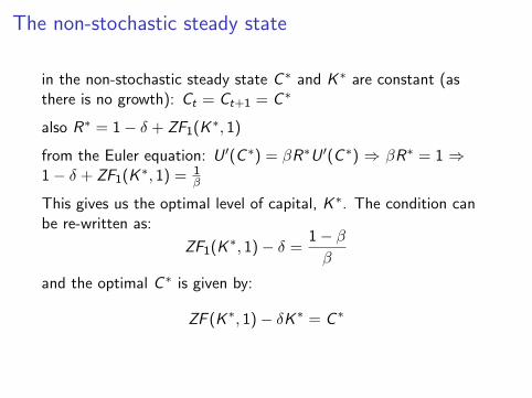
The non-stochastic steady state

in the non-stochastic steady state C ∗ and K ∗ are constant (asthere is no growth): Ct = Ct+1 = C ∗

also R∗ = 1− δ + ZF1(K ∗, 1)

from the Euler equation: U ′(C ∗) = βR∗U ′(C ∗) ⇒ βR∗ = 1 ⇒1− δ + ZF1(K ∗, 1) = 1

β

This gives us the optimal level of capital, K ∗. The condition canbe re-written as:

ZF1(K ∗, 1)− δ =1− ββ

and the optimal C ∗ is given by:

ZF (K ∗, 1)− δK ∗ = C ∗

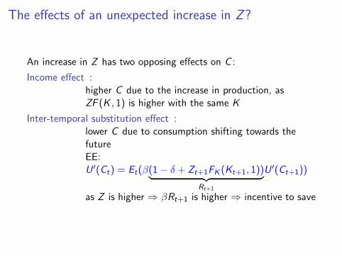
The effects of an unexpected increase in Z?

An increase in Z has two opposing effects on C :

Income effect :higher C due to the increase in production, asZF (K , 1) is higher with the same K

Inter-temporal substitution effect :lower C due to consumption shifting towards thefutureEE:U ′(Ct) = Et(β(1− δ + Zt+1FK (Kt+1, 1))︸ ︷︷ ︸

Rt+1

U ′(Ct+1))

as Z is higher ⇒ βRt+1 is higher ⇒ incentive to save

I net effect on C ambiguous, depends on the utility function

I S , I unambiguous increase

I Y increase, and further increase over time

I if increase in Z is transitory ⇒ C up less, I up more for lesstime

I good news: positive co-movements

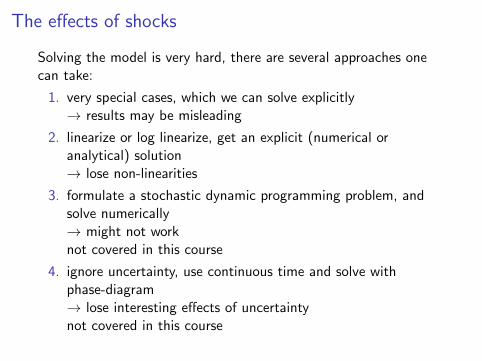
The effects of shocks

Solving the model is very hard, there are several approaches onecan take:

1. very special cases, which we can solve explicitly→ results may be misleading

2. linearize or log linearize, get an explicit (numerical oranalytical) solution→ lose non-linearities

3. formulate a stochastic dynamic programming problem, andsolve numerically→ might not worknot covered in this course

4. ignore uncertainty, use continuous time and solve withphase-diagram→ lose interesting effects of uncertaintynot covered in this course

1. A very special case

U(Ct) = logCt

ZtF (Kt , 1) = ZtKαt

δ = 1

HW: Find the solution to this problem, and give an intuition for itfor next week’s class.

2. Log-linearization

The first order conditions (FOCs) are a non-linear system ofequations. The main idea is that log-linearizing the model aroundits steady state gives a system of linear equations, which then canbe solved in many ways.Have to follow these steps:

1. write down the FOCs that govern the model

2. solve for the non-stochastic BGP

3. rewrite the model in terms of log deviations from thenon-stochastic BGP

4. study this alternative model, which is log-linear, and anapproximation of the original model around the non-stochasticBGP

We will go over this in detail two weeks from now.