Embed Size (px)
Citation preview

Graduate Macroeconomics I
Prof. Dietrich Vollrath
August 20th, 2007

ii
Contents
Graduate Macro in Fifteen Minutes or Less ix
1 The Consumption/Savings Decision 11.1 Properties of the Utility Function . . . . . . . . . . . . . . . . . . 2
1.1.1 Total Utility and Consumption Smoothing . . . . . . . . . 31.1.2 Uncertainty and Risk Aversion . . . . . . . . . . . . . . . 4
1.2 The Fisher Model . . . . . . . . . . . . . . . . . . . . . . . . . . . 61.2.1 Interest Rates . . . . . . . . . . . . . . . . . . . . . . . . . 81.2.2 Discount Rates . . . . . . . . . . . . . . . . . . . . . . . . 101.2.3 Modified Budget Constraints . . . . . . . . . . . . . . . . 111.2.4 Ricardian Equivalence . . . . . . . . . . . . . . . . . . . . 12
1.3 Uncertainty and Consumption . . . . . . . . . . . . . . . . . . . . 141.3.1 The Permanent Income Hypothesis . . . . . . . . . . . . . 141.3.2 Lifespan Uncertainty . . . . . . . . . . . . . . . . . . . . . 161.3.3 Precautionary Saving . . . . . . . . . . . . . . . . . . . . 16
1.4 Violations of Utility Assumptions . . . . . . . . . . . . . . . . . . 181.4.1 Habit Formation . . . . . . . . . . . . . . . . . . . . . . . 181.4.2 Intertemporal Consistency . . . . . . . . . . . . . . . . . . 19
1.5 Labor and Consumption Choices . . . . . . . . . . . . . . . . . . 191.5.1 The Basic Consumption/Leisure Problem . . . . . . . . . 201.5.2 Fluctuations and Consumption . . . . . . . . . . . . . . . 211.5.3 Labor, Consumption and Fluctuations . . . . . . . . . . . 22
2 The Mechanics of Economic Growth 252.1 Production Functions . . . . . . . . . . . . . . . . . . . . . . . . 252.2 The Solow Model . . . . . . . . . . . . . . . . . . . . . . . . . . . 28
2.2.1 Capital Accumulation . . . . . . . . . . . . . . . . . . . . 292.2.2 Golden Rule Saving . . . . . . . . . . . . . . . . . . . . . 312.2.3 Population Growth . . . . . . . . . . . . . . . . . . . . . . 322.2.4 Technical Change . . . . . . . . . . . . . . . . . . . . . . . 32
2.3 Human Capital . . . . . . . . . . . . . . . . . . . . . . . . . . . . 34
iii
iv CONTENTS
3 Essential Models of Dynamic Optimization 373.1 The T Period Fisher Model . . . . . . . . . . . . . . . . . . . . . 37
3.1.1 Infinitely Lived Agents . . . . . . . . . . . . . . . . . . . . 403.1.2 Dynamic Programming . . . . . . . . . . . . . . . . . . . 423.1.3 Lifespan Uncertainly and Insurance . . . . . . . . . . . . 453.1.4 Continuous Time Optimal Consumption . . . . . . . . . . 463.1.5 The Ramsey Model . . . . . . . . . . . . . . . . . . . . . . 493.1.6 Stochastic Income Shocks . . . . . . . . . . . . . . . . . . 553.1.7 Fixed Technological Growth . . . . . . . . . . . . . . . . . 58
3.2 The Overlapping Generations Model . . . . . . . . . . . . . . . . 593.2.1 The Basic Model . . . . . . . . . . . . . . . . . . . . . . . 593.2.2 Fixed Technological Growth . . . . . . . . . . . . . . . . . 633.2.3 Stochastic Income Shocks . . . . . . . . . . . . . . . . . . 64
4 Open Economy Macroeconomics 674.1 Open Economy Accounting . . . . . . . . . . . . . . . . . . . . . 674.2 Optimal Savings and the Interest Rate . . . . . . . . . . . . . . . 684.3 Growth in an Open Economy . . . . . . . . . . . . . . . . . . . . 70
4.3.1 Capital versus Assets . . . . . . . . . . . . . . . . . . . . 704.3.2 Non-tradable Human Capital . . . . . . . . . . . . . . . . 72
4.4 Optimal Consumption and Growth in an Open Economy . . . . . 73
5 Endogenous Growth Models 795.1 Empirics of Economic Development . . . . . . . . . . . . . . . . . 80
5.1.1 Growth and Development Accounting . . . . . . . . . . . 805.1.2 Growth Rates and Convergence . . . . . . . . . . . . . . . 815.1.3 Interest Rate Differentials . . . . . . . . . . . . . . . . . . 83
5.2 Basic Models . . . . . . . . . . . . . . . . . . . . . . . . . . . . . 845.2.1 The AK Model . . . . . . . . . . . . . . . . . . . . . . . . 845.2.2 Generalizing Endogenous Growth . . . . . . . . . . . . . . 865.2.3 Lucas’ Human Capital Model . . . . . . . . . . . . . . . . 90
5.3 Endogenous Technology Creation . . . . . . . . . . . . . . . . . . 915.3.1 Increasing Variety of Intermediate Goods . . . . . . . . . 925.3.2 Increasing Quality of Intermediate Goods . . . . . . . . . 96
5.4 Endogenous Population Growth . . . . . . . . . . . . . . . . . . . 1005.4.1 Lucas’ Malthusian Model . . . . . . . . . . . . . . . . . . 1015.4.2 Kremer’s Model of Long Run Population Growth . . . . . 1035.4.3 Optimal Fertility Choice . . . . . . . . . . . . . . . . . . . 104
A Solutions 107A.1 Solving for actual consumption (Example 4) . . . . . . . . . . . . 107A.2 Consumption Path in the Stochastic Ramsey Model . . . . . . . 108A.3 Social Security in the OLG Model (Example 17) . . . . . . . . . 109

CONTENTS v
B Problems 111B.1 Consumption/Savings . . . . . . . . . . . . . . . . . . . . . . . . 111B.2 Mechanical Growth . . . . . . . . . . . . . . . . . . . . . . . . . . 116B.3 Dynamic Optimization . . . . . . . . . . . . . . . . . . . . . . . . 118B.4 Open Economy . . . . . . . . . . . . . . . . . . . . . . . . . . . . 122B.5 Endogenous Growth . . . . . . . . . . . . . . . . . . . . . . . . . 124

vi CONTENTS

Preface
These notes are based mainly on the first-year graduate macro class of DavidWeil, with additional material from Sebnem Kalemli-Ozcan, Chris Carroll, andBrian Krauth that I’ve assimilated. There are sure to be errors and omissions,but those are mine alone.
vii

viii PREFACE

Graduate Macro in FifteenMinutes or Less
What Do We Care About?
Stuff. We care about how much stuff we have. Cars, boats, sandwiches,computers, clothes, and books among other things. The underlying assumptionin this class is that we derive all our utility from consuming things. So we careabout how much stuff we can consume at any given point in time. For themost part this is determined by the ability of the economy to produce stuff, andthat depends on things like the capital stock (things like factories and tools),the technology level (internal combustion engines versus horse-drawn carriages),and the efficiency of our financial system (how easy it is for people to get loansand invest in their businesses). In the long run these are all that matters forour standard of living.In intermediate macro, you would have learned how money gets used to buy
stuff. That is, money makes it easier for the right stuff to find the right personin the economy. However, for the purposes of this course, we’re going to ignoremoney (and all associated nominal concepts) completely. We will focus totallyon the real side of the economy - on how much stuff we can produce and howour consumption decisions today affect how much stuff we can have tomorrow.This doesn’t mean that we won’t be able to talk about business cycles, butthose cycles will have to be introduced through real shocks to the economy, asopposed being caused by the sluggish adjustment of the price level (a nominalthing).One could argue that only the long-run real aspect of the economy matters,
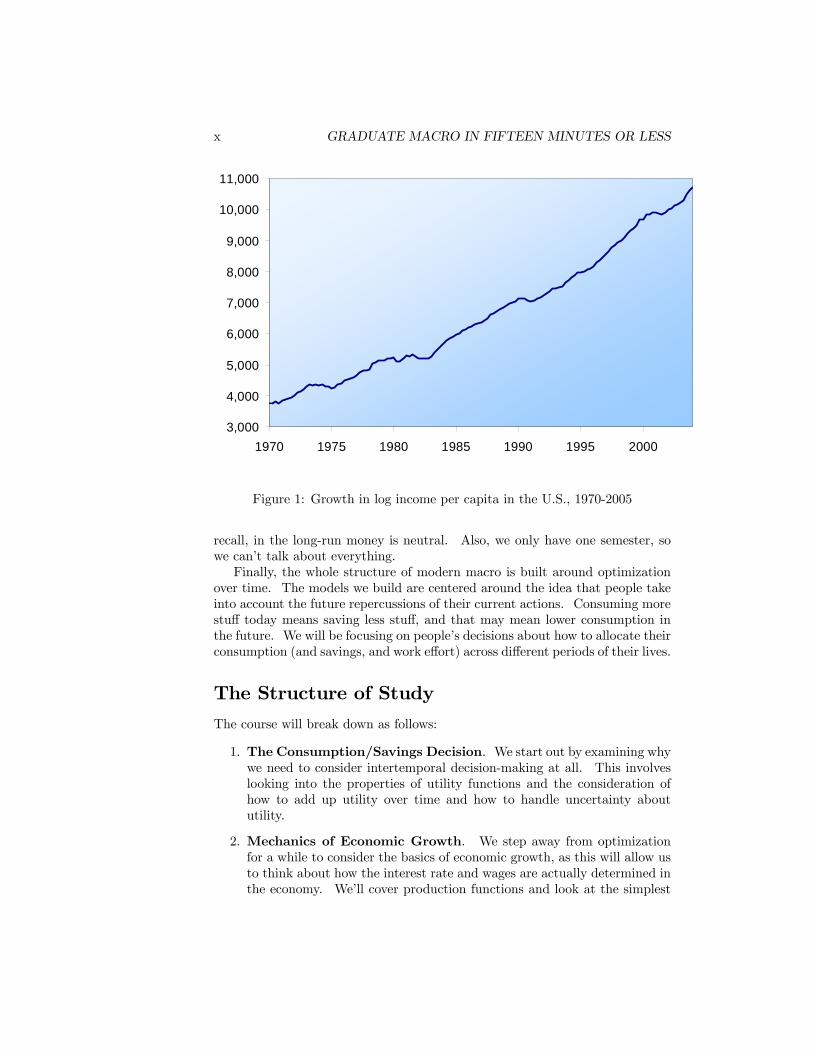
because it’s trend dominates the path of income. Figure 1 plots US real GDPsince 1970, and you can see that the trend growth swamps the cyclical move-ments. Understanding why the US trend growth was so big is arguably moreimportant that understanding why there were slight dips and surges in outputover the last 35 years. Across countries, the story seems much the same. Nige-ria isn’t poor because it has lots of recessions. Nigeria is poor because it’s longterm growth trend is essentially zero. This class will spend a lot of time talk-ing about the long-run growth trends of economies, and not very much aboutbusiness cycles. This is part of the reason why we ignore money, because if you
ix
x GRADUATE MACRO IN FIFTEEN MINUTES OR LESS
3,000
4,000
5,000
6,000
7,000
8,000
9,000
10,000
11,000
1970 1975 1980 1985 1990 1995 2000
Figure 1: Growth in log income per capita in the U.S., 1970-2005
recall, in the long-run money is neutral. Also, we only have one semester, sowe can’t talk about everything.Finally, the whole structure of modern macro is built around optimization
over time. The models we build are centered around the idea that people takeinto account the future repercussions of their current actions. Consuming morestuff today means saving less stuff, and that may mean lower consumption inthe future. We will be focusing on people’s decisions about how to allocate theirconsumption (and savings, and work effort) across different periods of their lives.
The Structure of StudyThe course will break down as follows:
1. The Consumption/Savings Decision. We start out by examining whywe need to consider intertemporal decision-making at all. This involveslooking into the properties of utility functions and the consideration ofhow to add up utility over time and how to handle uncertainty aboututility.
2. Mechanics of Economic Growth. We step away from optimizationfor a while to consider the basics of economic growth, as this will allow usto think about how the interest rate and wages are actually determined inthe economy. We’ll cover production functions and look at the simplest
xi
model of growth, the Solow model. These basics will then be useful forus in determining how individuals choose their consumption paths whenthey realize that their actions affect their future wages and interest rates.
3. Essential Models of Dynamic Optimization. This constitutes theheart of the class. We’ll look at the two workhorse model structures ofmodern macro: infinitely lived households and the overlapping generationsmodel. You’ll see how to mathematically set up these problems and whatthe results actually mean. We’ll cover solutions to these problems bothwith and without uncertainty about the future. Each model includes thepossibility of output growth over time.
4. The Open Economy Interpretation. The models we consider can beused to examine the external positions of economies in the world. We’llspend a short time showing how these positions come out of models thatare essentially identical to the previous models of dynamic optimization.As you’ll have plenty of chances for open economy macro later in yourtraining, this section won’t be terribly long.
5. Endogenous Growth Models. In these growth models, there areagain dynamically optimizing agents who take the mechanics of the growthprocess into account. In some cases, this won’t result in much of a dif-ference. The decisions that people make in these models are not simplybetween consumption versus savings, but also consumption versus researcheffort or consumption versus fertility. It also will introduce several com-mon ways of modelling firms in markets without perfect competition.
Goals of this Class
From my perspective, the goal is to teach you the important intuitions and me-chanics of modern macroeconomic research. This will allow you to start readingjournal articles - the medium through which you’ll actually teach yourself aboutmacroeconomic issues and facts. This subtle difference exists in all of your firstyear courses. A useful analogy for graduate school is this: first year coursesare similar to taking courses in a foreign language. You’ll learn syntax andgrammar, but you won’t be reading any great works of literature. Your upperlevel classes will introduce you to the ’classics’ in this new language. Finally,your own reading and research will be like finding a favorite author or genreand becoming fluent in this new language.This means that you might feel frustrated by this first year, because it focuses
a lot on mathematical techniques. This is not an indicator of how the professionfeels about research. Research economists are not impressed with technique.But you cannot speak about the important empirical issues of the day withouthaving this technique in place. So if you become frustrated, remind yourselfthat you are learning a new language, and you have to be patient.

xii GRADUATE MACRO IN FIFTEEN MINUTES OR LESS
From your perspective, the goals of this class are to learn enough macroeco-nomics to pass the comprehensive exams, and to understand the material wellenough that you can begin reading journal articles. I have several words ofadvice for you.
1. This is your job. You are a poorly paid or unpaid intern in the eco-nomics profession, but you are a member of this profession now. Actprofessionally and take this seriously.
2. This is not at all like your undergraduate classes. In those classes wewere trying to get across a small number of very general concepts. Ingraduate school we are trying to get across a large number of very spe-cific concepts. This requires you to study more evenly throughout thesemester, as opposed to cramming everything in just prior to tests.
3. Work with your classmates. You’ll all see different aspects of the problemsyou’ll be working on, and you’ll learn from their insights while they learnfrom yours. Also, it helps to have other people who like to make fun ofthe professor.
4. Ask questions and interrupt class. If you aren’t getting what I’m saying,stop me. Sometimes all it takes is for me to explain things in a slightlydifferent manner for things to click.
5. Don’t compare yourself to your classmates. You all have vastly differentbackgrounds and preparations for this. I am perfectly happy to giveall of you superior ratings on your comprehensive exams. There is nocompetition going on here.
6. Do not ask "will this be on the test?" The answer is always yes. If yourattitude is that you want to pass with as little effort as possible, then I’dsuggest you find another line of work. If you really want to get a PhD,you should want to know everything.
7. Do as many problems as possible. Do the homework problems I assign,and then do the extra problems you have access to. Do old midterm andfinal questions. Do old comprehensive questions. After you’ve done allthese problems, do them again. They are the best way to understand thismaterial and the best way to study for your comprehensive tests.
Chapter 1
The Consumption/SavingsDecision
In the beginning of macro, there was Keynes. And Keynes said that peopleconsumed according to the following function (roughly)
Ct = c0 + c1 (Yt − Tt) (1.1)
and that c1 represents the marginal propensity to consume. Notice that I’vewritten the Keynsian function with a time subscript, t. This is so that you cansee explicitly that consumption in period t is a function of disposable income inperiod t only. Future income, and expectations of future income, do not enterthe Keynsian consumption function. This generates several problems.
• Theoretical: It seems weird that future income doesn’t enter at all intosomeones decision to consume. Imagine that you know (with certainty)that you’ll receive $1,000,000 exactly one year from today. Wouldn’tyou consume more today? I would, but the Keynesian function in (1.1)says you won’t. It says that when you receive the million dollars, yourconsumption will rise, but not before. That seems weird, so we’re going towant to create a model of consumption that explicitly takes into accountfuture income.
• Empirical: The Keynsian consumption function implies that the savingsrate is affected by the income level
s =Y − T − C
Y − T= 1− C
Y − T= 1− c0
Y − T− c1 (1.2)
which shows that savings rates should rise with income. In the cross-section, this seems to work. Bill Gates saves a higher proportion of hisincome than you do, for example. But over time, this doesn’t seem tohold for countries or even necessarily for people. In Keynes defense, thedata didn’t exist at the time he was writing that could have showed himhis function didn’t work.
1
2 CHAPTER 1. THE CONSUMPTION/SAVINGS DECISION
So the basic Keynsian model of consumption is flawed, and this flaw comesprimarily from the fact that it does not account for the intertemporal nature ofthe savings decision. We want to construct a better model of savings, and todo so we’ll want to explicitly consider optimizing agents. That is, we want aneconomic model of savings in which someone is maximizing their utility subjectto a budget constraint. The budget constraint will involve the trade-off ofconsumption and savings, as opposed to the trade-off of good X and good Y.To start with, we’ll need to understand the nature of the utility function a littlebetter.
1.1 Properties of the Utility Function
Since we’ll be looking at an intertemporal utility function, we’ll need to dis-tinguish between overall utility and period-specific utility. The period specificutility function, call it U (ct), tells us how much the consumption you do inperiod t makes you happy. Sometimes the period specific utility is referred toas "felicity". We assume that U (ct) has the following properties
∂U (ct)
∂ct= U 0 (ct) > 0 (1.3)
∂2U (ct)
∂c2t= U 00 (ct) < 0 (1.4)
which are the basic properties that felicity is monotonically increasing in ct,and that felicity exhibits decreasing marginal utility. Without these properties,and especially without (1.4), there really isn’t anything interesting to say aboutdynamic optimization. The decreasing marginal utility of consumption hastwo important intepretations. First, a negative second derivative implies riskaversion - that is, people dislike uncertainty about consumption. Second, peoplelike to smooth their consumption over time - that is, they dislike jumps or spikesin consumption. These two properties are really just the same thing, and theyarise solely because of this negative second derivative.This might be easier to see in diagrams. If one maps utility against con-
sumption - U (c) versus c - then what we are assuming is that this is a concavefunction. Utility goes up with more consumption, but at a decreasing rate.Graphing the first derivative against c shows us a convex function, or marginalutility is large when c is low (and approaching infinity as c approaches zero) andmarginal utility is very low as c is high (and approaching zero as c approachesinfinity). Finally, graph the second derivative and you get a line that is alwaysnegative, and is close to negative infinity when c is close to zero and close tozero when c is very large.These graphs can give us the insight we need into why people are risk averse
and prefer smooth consumption. The essence of the intution is this: the averageof utilities is lower than the utility of the average. Take consumption of 10 andconsumption of 20, with an average of 15. The nature of the utility function
1.1. PROPERTIES OF THE UTILITY FUNCTION 3
tells us that the average of the utility of 10 and utility of 20 is less than theutility of 15. You can see this easily on the graph.
Definition 1 A way to measure the degree to which these effects bite is thecoefficient of relative risk aversion and it measures the curvature of theutility function. Relative risk aversion measures the elasticity of marginal utilitywith respect to consumption, or
−∂U0/∂C
U 0/C= −cU
00
U 0(1.5)
The larger is this value, the more rapidly marginal utility declines as consump-tion increases, or the utility curve "curves" more. The larger this curve, themore a person wants to smooth consumption and the more they’d pay to get ridof uncertainty.An alternate measure is the coefficient of absolute risk aversion, which isnot an elasticity. It is the percent change in utility given a unit change in c,or −U 00/U 0.
1.1.1 Total Utility and Consumption Smoothing
If U (ct) is felicity, or the utility of consumption in period t, what is lifetime, ortotal utlility? Let’s call this V . We will generally assume that V exhibits aproperty defined now as
Definition 2 Additive separability is a property of a utility function, andmeans that total utility V can be written as follows
V =TXt=0
U (ct) (1.6)
or in a continuous time situation that
V =
Z T
0
U (ct) dt (1.7)
The definition just given assumes that each period is just as important asany other. Later, we’ll introduce the idea of discounting to take into accountthe idea that you might not care about the future as much as today.Another way of looking at additive separability is that the marginal rate of
substitution between two periods is assumed to be independent of any otherperiod, or
MRSt,t+1 =U 0 (ct)
U 0 (ct+1)(1.8)
is independent of the marginal utility from any other period besides t and t+1.This makes the life of the dynamic optimizing much easier. However, it may
4 CHAPTER 1. THE CONSUMPTION/SAVINGS DECISION
not be a great assumption, and we’ll cover some situations later on where thisis violated1.So let’s think about what this additive separability means for how people
will allocate their consumption across periods. Let’s say you have $300 and twoperiods to spend it in. Your utility function is therefore V = U (c1) + U (c2).What is the optimal way to split up the $300? Given the additive nature, theanswer is to smooth it, or consume $150 in each period. To see this, considerwhat the marginal utility of consumption would look like in each period if youdidn’t smooth it. Let’s say you consume c1 = 200 and c2 = 100. Thenthe marginal utilities, given the properties we described above, relate like thisU 0 (200) < U 0 (100), or the marginal utility of first period consumption is lowerthan second period consumption. So you could move a dollar from period 1 toperiod 2 and have a net gain in utility. You could keep doing this until marginalutility was equalized across periods, which only happens when consumption is150 in each period.This shouldn’t be too surprising. The price of consumption in each period
is identical, so our intermediate microeconomist training tells us that the ratioof marginal utilities must equal the price ratio. In other words, the marginalutilities must be identical, and that can only happen when consumption is 150in each period.So one primary consequence of additive separability and the property of the
utility function is that people want to smooth consumption over time.
1.1.2 Uncertainty and Risk Aversion
Now let’s start over and consider utility only within one period, but there isuncertainly about what consumption might be. Suppose that I have a 50%chance of having $100 to consume and a 50% chance of having $200 to consume.How do I calculate my expected utility? There are two ways you could considerdoing this. One, you could take the utility of the expected level of consumptionwhich would look like this
V = U(0.5 ∗ 100 + 0.5 ∗ 200) (1.9)
and in this case you would be completely wrong. This is something thatpeople commonly make mistakes on, so stop and drill it into your head that thisis incorrect.The second method of computing expected utility is the right way and de-
serves its own definition.
Definition 3 The Von Neumann Mortgenstern (VNM) method of computingutility takes the expected utility of consumption, written as
V =NXi=1
piU (ci) (1.10)
1A simple example involves habit formation. If your utility depends not only on what youconsume today, but the size of this consumption relative to all your previous consumption,then additive separability doesn’t hold.
1.1. PROPERTIES OF THE UTILITY FUNCTION 5
where pi is the probability of situation i occuring (out of a possible N outcomes)and U (ci) is the utility of consumption in situation i. To make sense, we haveto have as well that
PNi=1 pi = 1. Note that VNM utility is very similar to the
simple additively separable utility function from the previous definition. Theyare both linear combinations of felicities.
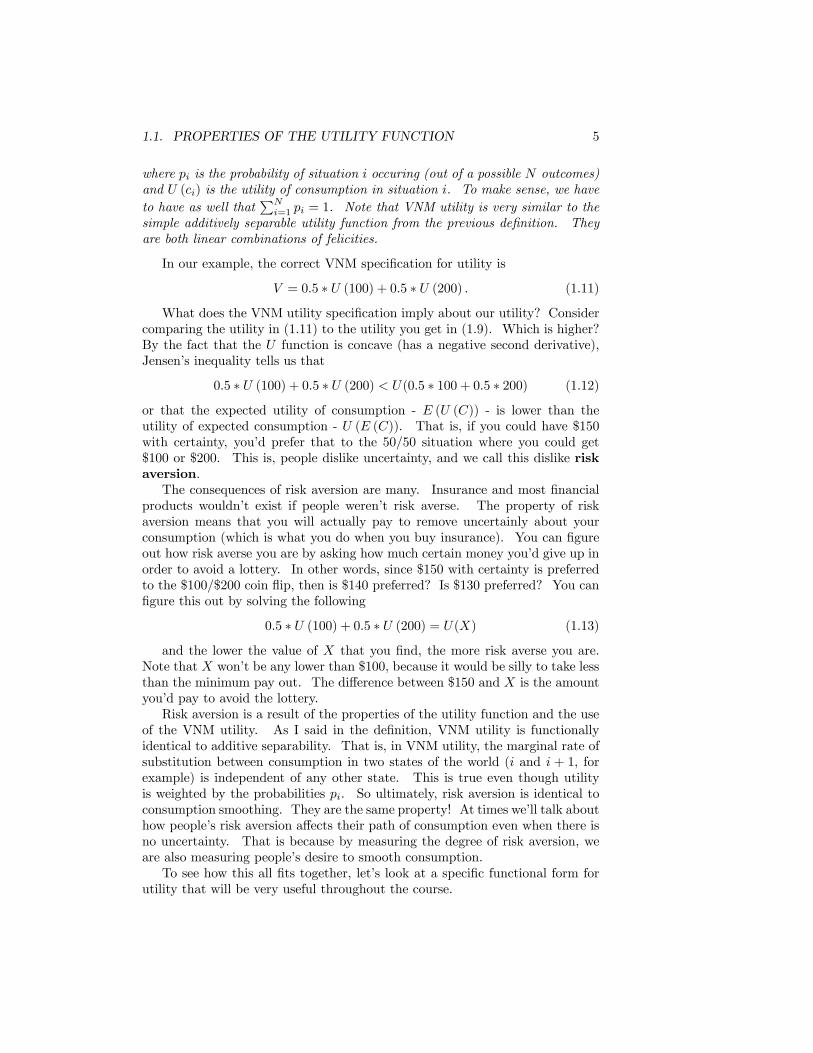
In our example, the correct VNM specification for utility is
V = 0.5 ∗ U (100) + 0.5 ∗ U (200) . (1.11)
What does the VNM utility specification imply about our utility? Considercomparing the utility in (1.11) to the utility you get in (1.9). Which is higher?By the fact that the U function is concave (has a negative second derivative),Jensen’s inequality tells us that
0.5 ∗ U (100) + 0.5 ∗ U (200) < U(0.5 ∗ 100 + 0.5 ∗ 200) (1.12)
or that the expected utility of consumption - E (U (C)) - is lower than theutility of expected consumption - U (E (C)). That is, if you could have $150with certainty, you’d prefer that to the 50/50 situation where you could get$100 or $200. This is, people dislike uncertainty, and we call this dislike riskaversion.The consequences of risk aversion are many. Insurance and most financial
products wouldn’t exist if people weren’t risk averse. The property of riskaversion means that you will actually pay to remove uncertainly about yourconsumption (which is what you do when you buy insurance). You can figureout how risk averse you are by asking how much certain money you’d give up inorder to avoid a lottery. In other words, since $150 with certainty is preferredto the $100/$200 coin flip, then is $140 preferred? Is $130 preferred? You canfigure this out by solving the following
0.5 ∗ U (100) + 0.5 ∗ U (200) = U(X) (1.13)
and the lower the value of X that you find, the more risk averse you are.Note that X won’t be any lower than $100, because it would be silly to take lessthan the minimum pay out. The difference between $150 and X is the amountyou’d pay to avoid the lottery.Risk aversion is a result of the properties of the utility function and the use
of the VNM utility. As I said in the definition, VNM utility is functionallyidentical to additive separability. That is, in VNM utility, the marginal rate ofsubstitution between consumption in two states of the world (i and i + 1, forexample) is independent of any other state. This is true even though utilityis weighted by the probabilities pi. So ultimately, risk aversion is identical toconsumption smoothing. They are the same property! At times we’ll talk abouthow people’s risk aversion affects their path of consumption even when there isno uncertainty. That is because by measuring the degree of risk aversion, weare also measuring people’s desire to smooth consumption.To see how this all fits together, let’s look at a specific functional form for
utility that will be very useful throughout the course.
6 CHAPTER 1. THE CONSUMPTION/SAVINGS DECISION
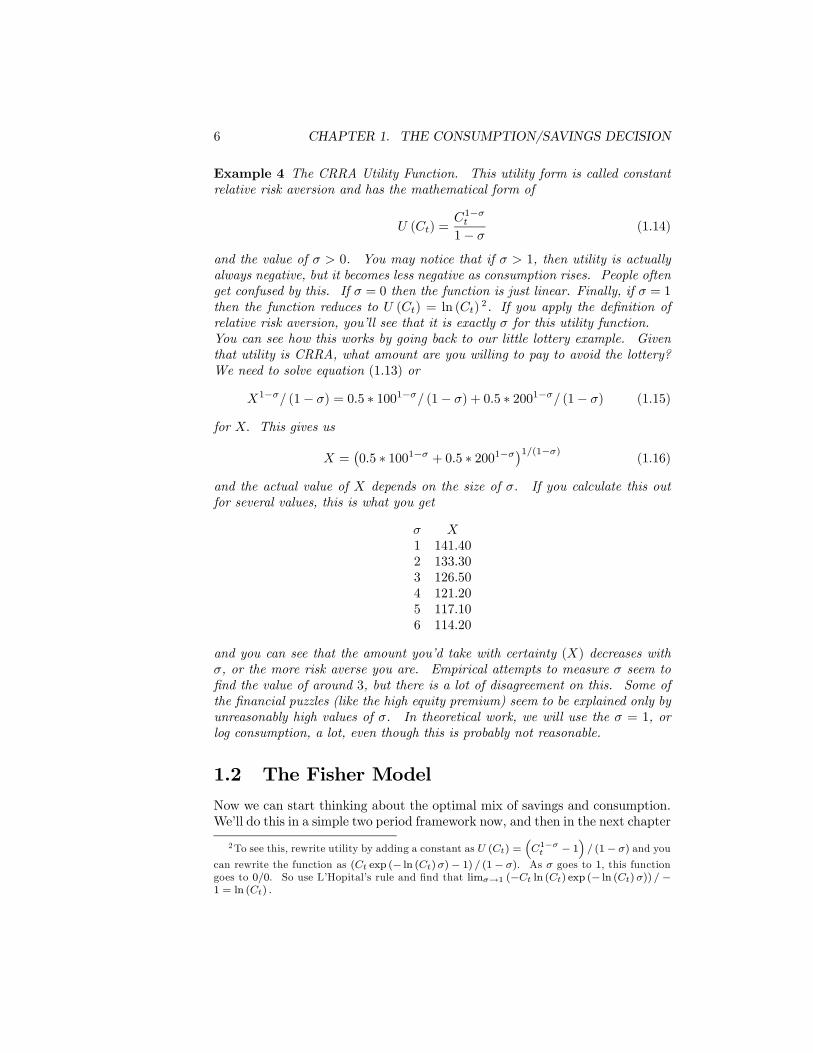
Example 4 The CRRA Utility Function. This utility form is called constantrelative risk aversion and has the mathematical form of
U (Ct) =C1−σt
1− σ(1.14)
and the value of σ > 0. You may notice that if σ > 1, then utility is actuallyalways negative, but it becomes less negative as consumption rises. People oftenget confused by this. If σ = 0 then the function is just linear. Finally, if σ = 1then the function reduces to U (Ct) = ln (Ct)
2 . If you apply the definition ofrelative risk aversion, you’ll see that it is exactly σ for this utility function.You can see how this works by going back to our little lottery example. Giventhat utility is CRRA, what amount are you willing to pay to avoid the lottery?We need to solve equation (1.13) or
X1−σ/ (1− σ) = 0.5 ∗ 1001−σ/ (1− σ) + 0.5 ∗ 2001−σ/ (1− σ) (1.15)
for X. This gives us
X =¡0.5 ∗ 1001−σ + 0.5 ∗ 2001−σ
¢1/(1−σ)(1.16)
and the actual value of X depends on the size of σ. If you calculate this outfor several values, this is what you get
σ X1 141.402 133.303 126.504 121.205 117.106 114.20
and you can see that the amount you’d take with certainty (X) decreases withσ, or the more risk averse you are. Empirical attempts to measure σ seem tofind the value of around 3, but there is a lot of disagreement on this. Some ofthe financial puzzles (like the high equity premium) seem to be explained only byunreasonably high values of σ. In theoretical work, we will use the σ = 1, orlog consumption, a lot, even though this is probably not reasonable.
1.2 The Fisher ModelNow we can start thinking about the optimal mix of savings and consumption.We’ll do this in a simple two period framework now, and then in the next chapter
2To see this, rewrite utility by adding a constant as U (Ct) = C1−σt − 1 / (1− σ) and you
can rewrite the function as (Ct exp (− ln (Ct)σ)− 1) / (1− σ). As σ goes to 1, this functiongoes to 0/0. So use L’Hopital’s rule and find that limσ→1 (−Ct ln (Ct) exp (− ln (Ct)σ)) /−1 = ln (Ct) .
1.2. THE FISHER MODEL 7
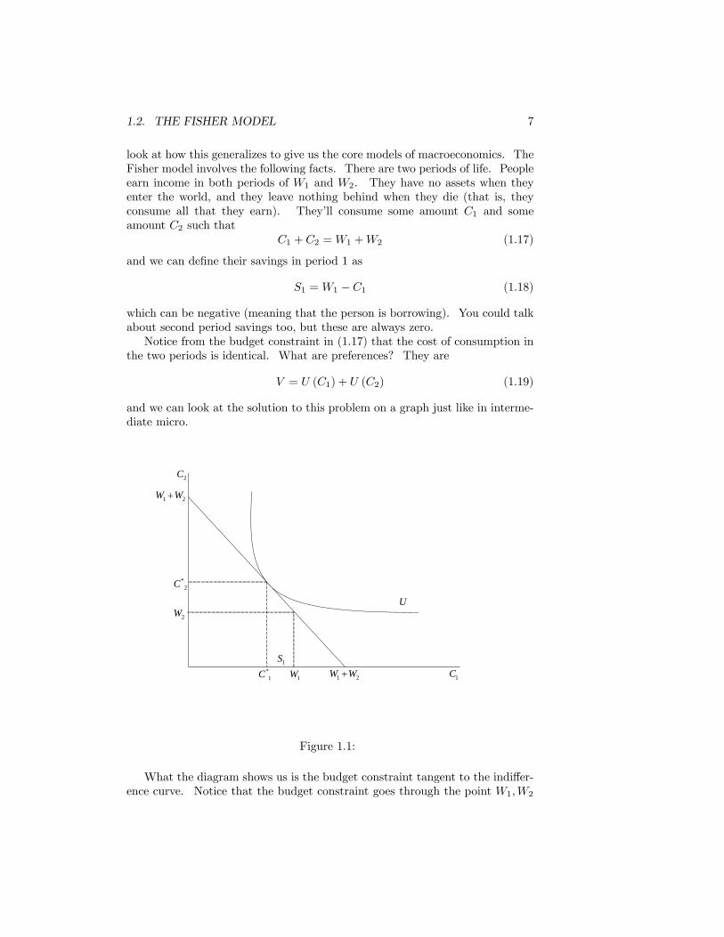
look at how this generalizes to give us the core models of macroeconomics. TheFisher model involves the following facts. There are two periods of life. Peopleearn income in both periods of W1 and W2. They have no assets when theyenter the world, and they leave nothing behind when they die (that is, theyconsume all that they earn). They’ll consume some amount C1 and someamount C2 such that
C1 + C2 =W1 +W2 (1.17)
and we can define their savings in period 1 as
S1 =W1 − C1 (1.18)
which can be negative (meaning that the person is borrowing). You could talkabout second period savings too, but these are always zero.Notice from the budget constraint in (1.17) that the cost of consumption in
the two periods is identical. What are preferences? They are
V = U (C1) + U (C2) (1.19)
and we can look at the solution to this problem on a graph just like in interme-diate micro.
1C
2C
1 2W W+
1 2W W+
U
*1C
*2C
1W
2W
1S
Figure 1.1:
What the diagram shows us is the budget constraint tangent to the indiffer-ence curve. Notice that the budget constraint goes through the point W1,W2
8 CHAPTER 1. THE CONSUMPTION/SAVINGS DECISION
because it is always feasible to just consume your endowment of income. It hasa slope of negative one, and it shows that you could consume all your incomein period 1 if you wanted to, or all income in period 2 if you wanted. There isno cost to moving income between periods here.The indifference curve (and you can confirm this shape is correct by looking
at how the marginal rate of substitution changes at different levels of C1 andC2), has the typical form. The tangency shows C1 < W1, which implies thatsavings is positive. So this person has large W1 relative to W2. and becausethey generally like to smooth consumption, they save something to consume inperiod 2. In fact, because the price of consumption is the same in each period,this person will consume exactly C1 = C2. The big kicker is that this doesn’tdepend at all on endowment, either its size or its distribution over time. Theabsolute size of C1 and C2 depends on the size of the total endowment, but noton the distribution of it.This is actually easier to see in math. So let’s set up the constrained
optimization problem for this person as a Lagrangian.
L = U (C1) + U (C2) + λ (W1 +W2 − C1 − C2) (1.20)
which has FOC of
∂L/∂C1 = U 0 (C1)− λ = 0 (1.21)
∂L/∂C2 = U 0 (C2)− λ = 0 (1.22)
∂L/∂λ = W1 +W2 − C1 − C2 = 0 (1.23)
and solving the first two FOC conditions together gives
U 0 (C1) = U 0 (C2) (1.24)
C1 = C2 (1.25)
or that consumption must be equal in both periods. Note that this part ofthe solution didn’t depend at all on using the budget constraint. Now combinethis with the budget constraint and you can get that
C1 = C2 =W1 +W2
2(1.26)
which is about what you’d expect.What happens to your consumption ifW2 goes up? Then C1 goes up and C2
goes up. Which is contrary to the Keynsian consumption function we startedthis chapter with. By taking the intertemporal nature of consumption intoaccount, we’ve found that the Keynsian version of the world doesn’t quite holdup. Consumption today depends crucially on income today and in the future.
1.2.1 Interest Rates
Now we start by adding some more realism. Let’s call r the real interest ratethat is earned on money saved in period 1 - or alternately the interest rate paid
1.2. THE FISHER MODEL 9
by people who borrow. Savings is still S1 = W1 − C1 but consumption in thesecond period is now C2 = S1 (1 + r)+W2 and we can combine this informationto get the new budget contraint which is
W1 +W2/ (1 + r) = C1 + C2/ (1 + r) (1.27)
and notice that now the price of consumption in the second period is actuallylower than that of consumption in the first period (because 1/ (1 + r) < 1).What does this do to consumption? Well, if we did another Lagrangian,
except with the new budget constraint, we’d get the following FOC
∂L/∂C1 = U 0 (C1)− λ = 0 (1.28)
∂L/∂C2 = U 0 (C2)− λ/ (1 + r) = 0 (1.29)
∂L/∂λ = W1 +W2/ (1 + r)− C1 − C2/ (1 + r) = 0 (1.30)
and solving the first two conditions together gives us
U 0 (C1) = (1 + r)U 0 (C2) (1.31)
C1 < C2 (1.32)
where the second step follows because 1 + r is greater than one, so that themarginal utility of C2 must be smaller than the marginal utility of C1, whichgiven the nature of the utility functions means that C1 < C2. So with interestinvolved, we see that now consumption tilts towards the second period. Noticeagain that this doesn’t depend on the size or distribution of the endowment.What about savings? Did savings rise or fall? This depends on what the
person was doing without interest rates.
• Person was saving. Recall that there are two effects of a price change: theincome and substitution effects. The decrease in price of C2 is like havinga higher income, so that this pushes up consumption in period one andperiod two. However, the substitution effect says that the person shouldstart consuming more C2 and less C1 (which we saw). So the effect on C1is ambiguous, and therefore the effect on S1 is ambiguous. This analysisholds in any case where the interest rate is increasing and the person is afirst period saver.
• Person was borrowing. In this case the income effect is negative for bothC1 and C2. The substitution effect is negative as well for C1 when rgoes up, so that it is unambiguous that C1 falls and savings goes up (orborrowing goes down).
Example 5 We can complicate things slightly more in macro because we actu-ally have that the price of one good (r) affects your actual income (think of thisas an endowment effect). So we can decompose the effects of a change in r
10 CHAPTER 1. THE CONSUMPTION/SAVINGS DECISION
into more parts. Let’s take a typical CRRA utility function and solve it with abudget constraint. The Euler equation we get is
C2 = (1 + r)1/σ
C1 (1.33)
and a budget constraint of
C1 +C21 + r
= Y1 +Y21 + r
(1.34)
yields the following answer for first period consumption.
C1 =1
1 + (1 + r)1/σ−1
∙Y1 +
Y21 + r
¸. (1.35)
First, notice that consumption in the first period is a constant fraction of totallifetime income. If we hold the total Y1 + Y2
1+r constant but move around thepattern of income, first period consumption doesn’t change. So back to thedecomposition. The tension in between the income and substitution effects isfound in the (1 + r)1/σ−1 term. If 1/σ − 1 > 0, or σ < 1, then the substitutioneffect dominates, and an increase in r will shift consumption towards period 2because people are really willing to substitute. If 1/σ − 1 < 0, then the incomeeffect dominates and an increase in r will raise current consumption. There isa third effect, though, that we can see from this equation. That is the wealtheffect - or the fact that 1 + r going up means that the PDV of lifetime earningsis now lower. So while the income effect might win out, and it normally willgiven that our assumption is that σ > 1, we still might have current consumptionfalling if income is mainly gained in the future.
1.2.2 Discount Rates
So far we’ve assumed that the utility of consuming in period 2 is just as good asthe utility of consuming in period 1. Except that you have to wait until period2 to do the consumption, and this delay might make it less satisfying today.That is, you are optimizing today, and delaying consumption means that youhave to wait, which may not be very fun. So let’s say that now we discountfuture utility by the factor of θ in the following manner.
V = U (C1) +U (C2)
1 + θ(1.36)
which affects the slope of the utility function (but does nothing to the budgetconstraint). As θ goes up, this makes utility in the second period less and lessdesirable, and the indifference curves start to slope more steeply, pushing theoptimal choice towards C1. If you set up the Lagrangian again, including theinterest rate and the discount rate, you get the following FOC
1.2. THE FISHER MODEL 11
∂L/∂C1 = U 0 (C1)− λ = 0 (1.37)
∂L/∂C2 = U 0 (C2) / (1 + θ)− λ/ (1 + r) = 0 (1.38)
∂L/∂λ = W1 +W2/ (1 + r)− C1 − C2/ (1 + r) = 0 (1.39)
which can be solved for
U 0 (C1) =(1 + r)
(1 + θ)U 0 (C2) (1.40)
C1 < C2 ⇐⇒(1 + r)
(1 + θ)> 1 (1.41)
C1 > C2 ⇐⇒(1 + r)
(1 + θ)< 1 (1.42)
and we see that the pattern of consumption depends on the relative sizes ofr and θ. Also, if r = θ, then we’re right back at having C1 = C2, although fora much different reason than we started with.
1.2.3 Modified Budget Constraints
So far we’ve assumed that the consumer can borrow and save at the identicalinterest rate. What if there are differential interest rates so that rb > rs orthe real interest rate to borrow exceeds that of savings. Then the budget setis kinked and there are three possible optima. The indifference curve couldbe tangent to one of the arms, so that the differential doesn’t matter. Or thesolution could be to cosume at the kink point. The interesting thing about thisis that if either interest rate changes, consumption and savings may not changeat all, meaning that savings are invariant to interest rates. You’ll have someproblems to do that involve this modification.Another possibility is that the consumer is liquidity constrained, and cannot
borrow but can only save (something like being a college student). Now thebudget set has a vertical section below the endowment point, and the individualcannot set C1 > W1. Does this constraint bind? Only if the person wouldhave borrowed in the first place. If so, then they’ll consume at the kink pointagain, and any increase in their W1 will translate one for one into increases inC1, giving something like a Keynsian relationship.This section seems really short, and you might be inclined to think that
this means that modified budget constraints are relatively unimportant. Thiscouldn’t be further from the truth. Much of what is added to consumptiontheory to make it match the facts involves limitations to peoples ability toborrow or save. This kind of problem requires you to think a lot about peoplesoptimization - and can’t always be solved in a straightforward Lagrangian orwith calculus. Which is why it makes for great problem sets and test questions.Be warned.
12 CHAPTER 1. THE CONSUMPTION/SAVINGS DECISION
1.2.4 Ricardian Equivalence
This is a concept that David Ricardo originally mentioned, and then dismissed.Robert Barro revived the discussion in modern times by asking whether gov-ernment debt actually constituted wealth. To see what they were both talkingabout, consider a two period Fisher world, but now you have to pay taxes ineach period (the government collects this money and throws it in the ocean, sothere is no affect of government spending here). Your budget constraint is now
C1 +C21 + r
=W1 − T1 +W2 − T21 + r
(1.43)
which is no different than saying that the actual size of your wages changed.From before, we know that this will have no effect on the optimal consumptionpath, and that we should still have U 0 (C1) /U 0 (C2) = (1 + r) / (1 + θ), whichshows that the size of your wages and their distribution doesn’t affect youroptimal path.What happens if we introduce a change in the tax collection scheme? We
will say that taxes change as follows
∆T1 = −Z∆T2 = (1 + r)Z
or that the present value of taxes collected is unchanged. If Z were positive,then taxes are being cut today, and raised in the future. Plug this into thebudget constraint and you get
C1 +C21 + r
=W1 − [T1 − Z] +W2 − [T2 + (1 + r)Z]
1 + r
and if you do the algebra you see that the Z0s cancel out completely and you’releft with the same exact budget constraint as before. What happens to first pe-riod savings? Well, the Euler equation is identical, and the budget constraint isidentical to before the change in taxes, so your consumption must be completelyunchanged by this change in taxes. Then
S1 =W1 − T1 − C1 (1.44)
and C1 is fixed. So any decrease in taxes must raise savings by the same amount.People do not choose to consume any of their tax break. Does this increase insavings have any effect on the capital stock? No. Because to finance the taxcut, the government has to issue bonds, on which it will pay an interest rateof r. So from an individuals perspective, these bonds are wealth, in that theyprovide a way of earning r on their savings. But from the aggregate perspectivethey are not wealth, because they are just government liabilities which have tobe paid back by the economy later.So the upshot is that if taxes go down today, that should have no effect on
consumption because people are far-sighted enough to understand that they’ll
1.2. THE FISHER MODEL 13
need to pay higher taxes in the future. Ricardian equivalence is about thetiming of taxes - it does not say that government spending will have no effecton consumption. So if the government raises spending, this will lower yourabsolute consumption levels as they take more money out of the system. Butit won’t matter to you whether this new spending is financed by direct taxesor by bonds. The optimal path of consumption will remain the same, only thelevel will change.There a host of objections to Ricardian equivalence:
1. Different interest rates for government borrowing and individual saving/borrowing
2. If people are liquidity constrained in the first period, then governmentborrowing (taxes going down) will raise their consumption
3. If people are myopic it doesn’t work. Probably true, but how exactly doyou model myopia?
4. If people will be dead before they have to pay back the taxes, then the taxdecrease will allow them to increase their consumption. Later generationswill pay the extra taxes and consume less. This has raised a lot ofdebate and runs into a whole long-winded debate about intergenerationalrelations. Before touching on that, note that most of the present valueof a tax cut will be paid back by people alive today, so RE should holdpretty close to absolutely.The intergenerational argument in defense of RE is that we see peoplegiving bequests when they die, so they must care about their children’sconsumption. The tax decrease is like taking money away from theirchildren and giving it to them, so they’ll just leave that as a bequest fortheir children and consumption won’t change in the current period.A lot of people attack this reasoning. Parents may not get utility fromtheir childrens consumption but from the actual giving of a bequest, andthen the bequest is kind of like consumption for the parent and when taxesfall they’ll increase both their bequest and their income. Alternately, youcould argue that most bequests are accidental, not intentional, becausepeople die before they expect to.
A last thought about RE. If people were completely myopic and neverexpected to pay back their tax cut, what would happen. If they followedour usual model of consumption smoothing, they would still only raise theirconsumption by a little, spreading the tax decrease out over their whole lives(remember that the timing of your income doesn’t matter). So RE would bevery close to true. Compare that to Keynsian consumption, where people wouldconsume almost the whole tax cut immediately.
14 CHAPTER 1. THE CONSUMPTION/SAVINGS DECISION
1.3 Uncertainty and ConsumptionWe now have the basic framework in place to analyze a lot of different prob-lems relating to the consumption/savings decision and how uncertainty changesthings.
1.3.1 The Permanent Income Hypothesis
The permanent income hypothesis of Milton Friedman developed two modernlines of thinking about consumption. First, he suggested that uncertain incomeshould be treated different from certain income. Second, he suggested thatpeople should take into account their whole lifetime path of income and con-sumption into their decision process (extending the Fisher model to T periods,and similar to Modigliani’s life-cycle hypothesis). In this section, we’ll con-sider the first point - the role of uncertainty in income. Friedman proposedthat you could divide income into two components: the permanent part and thetransitory part
Y = Y P + Y T .
The permanent component of income is what you could think of as averagelifetime income, or your expected income in any period. The transitory com-ponent is al those additional random factors that occur. So permanent incomemay be your expected salary (which can be rising, but is generally known andyou expect to receive it) while transitory income would be like winning a lotteryor having your car break down (the shock can be either positive or negative,but is not expected).What Friedman proposed was that only the permanent component of in-
come should matter for consumption. The transitory component has a meanof zero (if it didn’t, then it would have a permanent component to it), so thatyou expect over your life that the shocks to income will balance out. Whichmeans that if you recieve a positive shock, you’ll save it to cover yourself whenyou have a negative shock. So no transitory shock will ever affect your con-sumption. Any change in permanent income, though, will materially impactyour consumption because you are raising your expectation of all your futureincomes. So consumption looks like this
C = αY P
Over the long run, as income increases, so does consumption. So thisseems to match with Keynes. What about in the short run, or looking acrosshouseholds? If all the variation in income in the short run was from transitoryincome shocks, then there would be NO relationship between C and Y in theshort run. As more and more of the variation across households is explained bypermanent income differences, then C would start to show a positive relationshipwith Y .This matches the data much better than Keynes did, who predicted that the
short run and long run relationship between C and Y was the same. The data
1.3. UNCERTAINTY AND CONSUMPTION 15
shows that C is related to Y much more strongly in the long run than in theshort run. And this we attribute to the larger transitory component of incomein the short run. This type of thinking leads us into the uncertainty portionof consumption theory, and we’ll see how more variability in income leads todifferent savings behavior.Let’s think about a really simple two period model. In the first period you
earn W with certainty, and in the second your earn W + δ, where δ is somerandom variable (transitory income) with mean zero. Your expected utility is
EV = U (C1) +E (U (C2)) (1.45)
and the budget constraint can be written as
C2 = 2W − C1 + δ (1.46)
so that utility is now
EV = U (C1) +E¡U¡2W − C1 + δ
¢¢.
You can maximize this over C1 and you’ll find that you get
U 0 (C1) = EU 0¡2W − C1 + δ
¢= EU 0 (C2)
which tells us that you’ll equate marginal utility of consumption in period onewith the expected marginal utility of consumption in period 2. Not surpris-ing, really. Your income will vary in period 2, but you still want to smoothconsumption in the same manner as before. This is highly important to note.From this Euler equation - uncertainty has not changed anything fundamentalabout how you dynamically optimize. It doesn’t indicate that your behavioractually changes (we’ll get to if and why it might). All uncertainty shoulddo is reduce your overall utility, but it won’t necessarily change how much youconsume.Recall a handy rule from the world of statistics. Namely, that the actual
realization of a random variable can be written as follows
X = E (X) + ε (1.47)
where ε is a random variable with mean zero (and is different than the δ randomvariable). So we can write
U 0 (C2) = EU 0 (C2) + ε (1.48)
and then use (1.48) in (??) to show that
U 0 (C2) = U 0 (C1) + ε (1.49)
or that the marginal utility of consumption follows a random walk. If youactually have positive r and θ, then you’d get an expression that shows thatmarginal utility should follow a random walk with drift.
16 CHAPTER 1. THE CONSUMPTION/SAVINGS DECISION
So what does all this do for us? Well, equation (1.49) tells us that the changein marginal utility between periods - U 0 (C2)−U 0 (C1) - should be random. If thechange in actual marginal utility between periods is random, then the change inconsumption itself should be random. More specifically, there is no informationout there in the world that should be able to predict how your consumption willchange from period to period.This is the test of the PIH proposed by Robert Hall. Suppose you have a set
of variables Z that predict changes in income (things like past income, the stockmarket, consumer confidence, etc..). These Z items may also predict the levelof consumption in any period. But these Z factors should have no relationshipto the change in consumption between periods. If you had any Z variable thatpredicted changes in consumption, then the PIH would be violated.The great thing about Hall’s idea is that is doesn’t require the econometrician
to know much about how the consumption decision is being made. For example,we don’t have to know anything about how expectations of future income aremade.
1.3.2 Lifespan Uncertainty
So far, we’ve assumed that there was certain end date of someones life. Whatif we allow for the proabability of dying prior to period 2? Let’s start with areally simple example. Let’s say that I have a two period Fisher model, butthat I have a 1− p percent change of dying before I get to consume anything inperiod 2. Then what is my expected utility?
EV = U (C1) + p ∗ U (C2)1 + θ
(1.50)
which still has a pure time discount of θ, but has this 0.5 term to account for thefact that I only have half a chance of living to consume. Well, this is essentiallyjust a modification of the discount rate, so my answer should be that
U 0 (C1)
U 0 (C2)=
µ1 + r
1 + θ
¶p (1.51)
and what this tells me is that, holding r and θ constant, I should scale downU 0 (C1) /U
0 (C2) by the factor p. This means I should raise first period con-sumption (so that marginal utility falls) and lower second period consumption(so that marginal utility rises). Which isn’t surprising. If I might be dead nextyear, I don’t want to save too much money because I might not get to enjoy itat all.
1.3.3 Precautionary Saving
We know that uncertainty makes you worse off. That’s a result of havingU 00 < 0 which implies that E (U (C)) < U (E (C)). But the fact that you areworse off with uncertainty doesn’t necessarily mean you’ll make any different
1.3. UNCERTAINTY AND CONSUMPTION 17
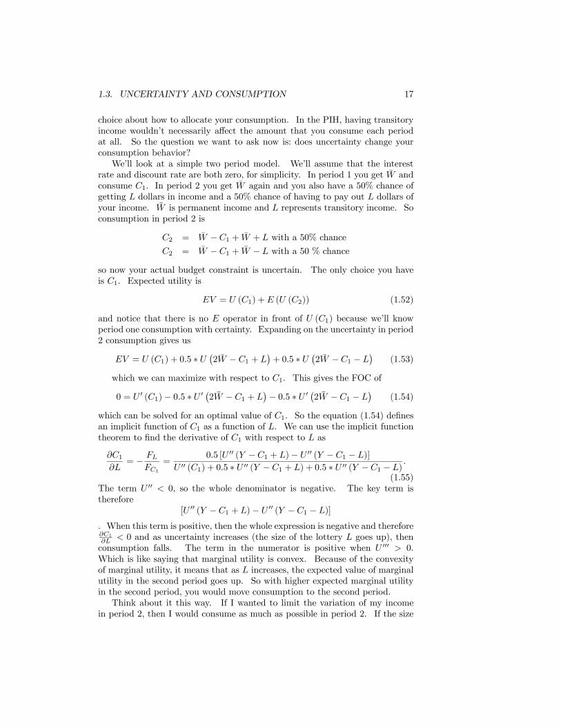
choice about how to allocate your consumption. In the PIH, having transitoryincome wouldn’t necessarily affect the amount that you consume each periodat all. So the question we want to ask now is: does uncertainty change yourconsumption behavior?We’ll look at a simple two period model. We’ll assume that the interest
rate and discount rate are both zero, for simplicity. In period 1 you get W andconsume C1. In period 2 you get W again and you also have a 50% chance ofgetting L dollars in income and a 50% chance of having to pay out L dollars ofyour income. W is permanent income and L represents transitory income. Soconsumption in period 2 is
C2 = W − C1 + W + L with a 50% chance
C2 = W − C1 + W − L with a 50 % chance
so now your actual budget constraint is uncertain. The only choice you haveis C1. Expected utility is
EV = U (C1) +E (U (C2)) (1.52)
and notice that there is no E operator in front of U (C1) because we’ll knowperiod one consumption with certainty. Expanding on the uncertainty in period2 consumption gives us
EV = U (C1) + 0.5 ∗ U¡2W − C1 + L
¢+ 0.5 ∗ U
¡2W − C1 − L
¢(1.53)
which we can maximize with respect to C1. This gives the FOC of
0 = U 0 (C1)− 0.5 ∗ U 0¡2W − C1 + L
¢− 0.5 ∗ U 0
¡2W − C1 − L
¢(1.54)
which can be solved for an optimal value of C1. So the equation (1.54) definesan implicit function of C1 as a function of L. We can use the implicit functiontheorem to find the derivative of C1 with respect to L as
∂C1∂L
= − FLFC1
=0.5 [U 00 (Y − C1 + L)− U 00 (Y − C1 − L)]
U 00 (C1) + 0.5 ∗ U 00 (Y − C1 + L) + 0.5 ∗ U 00 (Y − C1 − L).
(1.55)The term U 00 < 0, so the whole denominator is negative. The key term istherefore
[U 00 (Y − C1 + L)− U 00 (Y − C1 − L)]
. When this term is positive, then the whole expression is negative and therefore∂C1∂L < 0 and as uncertainty increases (the size of the lottery L goes up), thenconsumption falls. The term in the numerator is positive when U 000 > 0.Which is like saying that marginal utility is convex. Because of the convexityof marginal utility, it means that as L increases, the expected value of marginalutility in the second period goes up. So with higher expected marginal utilityin the second period, you would move consumption to the second period.Think about it this way. If I wanted to limit the variation of my income
in period 2, then I would consume as much as possible in period 2. If the size
18 CHAPTER 1. THE CONSUMPTION/SAVINGS DECISION
of the L were $1000, then if I had saved only $1000, I would be looking at a50/50 chance of either zero dollars or $2000, which seems like a big difference.However, if I had saved $1,000,000, then I would have a 50/50 chance of either$1,001,000 or $999,000, and I’d be pretty well off with either of those results.So to limit the relative variability of my utility in period 2, I transfer money tothat period. In essence, I buy certainty in period 2 with money from period 1.This result holds for models beyond two periods as well. As long as U 000 > 0,
you get precautionary saving, and this holds for things like log utility or anyCRRA utility function. On the other hand, if you have quadratic utility, thenU 000 = 0 and there is no precautionary saving. The person in this case acts asif income in the second period were certain to arrive at its expected value. Theuncertainty doesn’t alter his optimal consumption choice.
1.4 Violations of Utility Assumptions
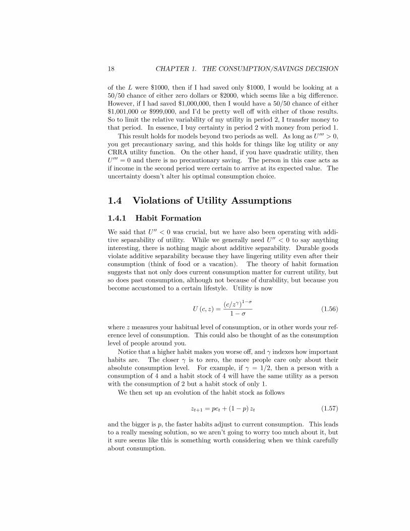
1.4.1 Habit Formation
We said that U 00 < 0 was crucial, but we have also been operating with addi-tive separability of utility. While we generally need U 00 < 0 to say anythinginteresting, there is nothing magic about additive separability. Durable goodsviolate additive separability because they have lingering utility even after theirconsumption (think of food or a vacation). The theory of habit formationsuggests that not only does current consumption matter for current utility, butso does past consumption, although not because of durability, but because youbecome accustomed to a certain lifestyle. Utility is now
U (c, z) =(c/zγ)1−σ
1− σ(1.56)
where z measures your habitual level of consumption, or in other words your ref-erence level of consumption. This could also be thought of as the consumptionlevel of people around you.Notice that a higher habit makes you worse off, and γ indexes how important
habits are. The closer γ is to zero, the more people care only about theirabsolute consumption level. For example, if γ = 1/2, then a person with aconsumption of 4 and a habit stock of 4 will have the same utility as a personwith the consumption of 2 but a habit stock of only 1.We then set up an evolution of the habit stock as follows
zt+1 = pct + (1− p) zt (1.57)
and the bigger is p, the faster habits adjust to current consumption. This leadsto a really messing solution, so we aren’t going to worry too much about it, butit sure seems like this is something worth considering when we think carefullyabout consumption.
1.5. LABOR AND CONSUMPTION CHOICES 19
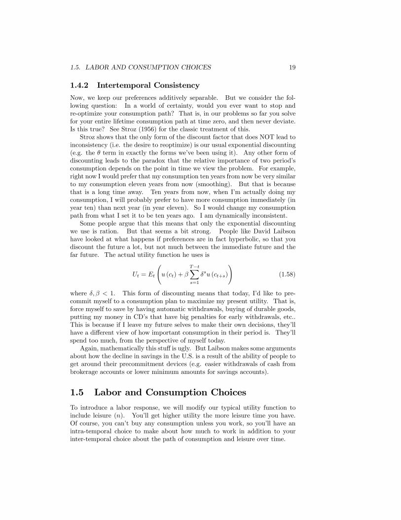
1.4.2 Intertemporal Consistency
Now, we keep our preferences additively separable. But we consider the fol-lowing question: In a world of certainty, would you ever want to stop andre-optimize your consumption path? That is, in our problems so far you solvefor your entire lifetime consumption path at time zero, and then never deviate.Is this true? See Stroz (1956) for the classic treatment of this.Stroz shows that the only form of the discount factor that does NOT lead to
inconsistency (i.e. the desire to reoptimize) is our usual exponential discounting(e.g. the θ term in exactly the forms we’ve been using it). Any other form ofdiscounting leads to the paradox that the relative importance of two period’sconsumption depends on the point in time we view the problem. For example,right now I would prefer that my consumption ten years from now be very similarto my consumption eleven years from now (smoothing). But that is becausethat is a long time away. Ten years from now, when I’m actually doing myconsumption, I will probably prefer to have more consumption immediately (inyear ten) than next year (in year eleven). So I would change my consumptionpath from what I set it to be ten years ago. I am dynamically inconsistent.Some people argue that this means that only the exponential discounting
we use is ration. But that seems a bit strong. People like David Laibsonhave looked at what happens if preferences are in fact hyperbolic, so that youdiscount the future a lot, but not much between the immediate future and thefar future. The actual utility function he uses is
Ut = Et
Ãu (ct) + β
T−tXs=1
δsu (ct+s)
!(1.58)
where δ, β < 1. This form of discounting means that today, I’d like to pre-commit myself to a consumption plan to maximize my present utility. That is,force myself to save by having automatic withdrawals, buying of durable goods,putting my money in CD’s that have big penalties for early withdrawals, etc..This is because if I leave my future selves to make their own decisions, they’llhave a different view of how important consumption in their period is. They’llspend too much, from the perspective of myself today.Again, mathematically this stuff is ugly. But Laibson makes some arguments
about how the decline in savings in the U.S. is a result of the ability of people toget around their precommitment devices (e.g. easier withdrawals of cash frombrokerage accounts or lower minimum amounts for savings accounts).
1.5 Labor and Consumption ChoicesTo introduce a labor response, we will modify our typical utility function toinclude leisure (n). You’ll get higher utility the more leisure time you have.Of course, you can’t buy any consumption unless you work, so you’ll have anintra-temporal choice to make about how much to work in addition to yourinter-temporal choice about the path of consumption and leisure over time.
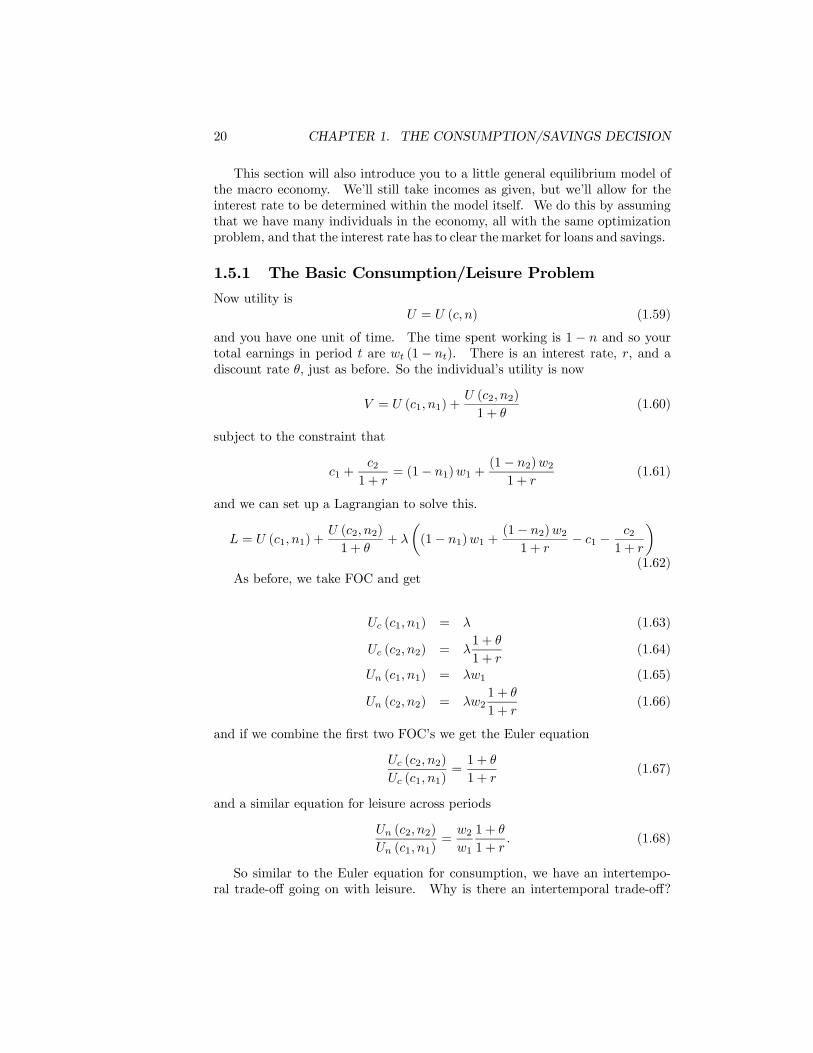
20 CHAPTER 1. THE CONSUMPTION/SAVINGS DECISION
This section will also introduce you to a little general equilibrium model ofthe macro economy. We’ll still take incomes as given, but we’ll allow for theinterest rate to be determined within the model itself. We do this by assumingthat we have many individuals in the economy, all with the same optimizationproblem, and that the interest rate has to clear the market for loans and savings.
1.5.1 The Basic Consumption/Leisure Problem
Now utility isU = U (c, n) (1.59)
and you have one unit of time. The time spent working is 1 − n and so yourtotal earnings in period t are wt (1− nt). There is an interest rate, r, and adiscount rate θ, just as before. So the individual’s utility is now
V = U (c1, n1) +U (c2, n2)
1 + θ(1.60)
subject to the constraint that
c1 +c21 + r
= (1− n1)w1 +(1− n2)w21 + r
(1.61)
and we can set up a Lagrangian to solve this.
L = U (c1, n1) +U (c2, n2)
1 + θ+ λ
µ(1− n1)w1 +
(1− n2)w21 + r
− c1 −c21 + r
¶(1.62)
As before, we take FOC and get
Uc (c1, n1) = λ (1.63)
Uc (c2, n2) = λ1 + θ
1 + r(1.64)
Un (c1, n1) = λw1 (1.65)
Un (c2, n2) = λw21 + θ
1 + r(1.66)
and if we combine the first two FOC’s we get the Euler equation
Uc (c2, n2)
Uc (c1, n1)=1 + θ
1 + r(1.67)
and a similar equation for leisure across periods
Un (c2, n2)
Un (c1, n1)=
w2w1
1 + θ
1 + r. (1.68)
So similar to the Euler equation for consumption, we have an intertempo-ral trade-off going on with leisure. Why is there an intertemporal trade-off?
1.5. LABOR AND CONSUMPTION CHOICES 21
Because the amount of leisure I take affects the earnings I make, and thereforeI want my leisure to fit into my optimal consumption path. Notice, though,that optimal leisure also depends on the relative wage levels. Wages are howwe translate the leisure choice into consumption, so the marginal cost of leisurein a period depends on its wage.I can use the leisure FOC to think about the labor response to shocks. If
there is a positive shock to output in period 1, then w2 goes up, and the marginalcost of leisure is high, so I take less. In other words, I work more when thereturn to work is higher. So labor is procyclical, and output goes up not onlybecause of the positive productivity shock, but also because of increased laboreffort.But that’s not all, we also have to consider the static FOC that relates
consumption and leisure within a given period. Consider the first and thirdconditions above which solve to
Un (c1, n1) = w1U (c1, n1) (1.69)
and says that the marginal utility of consumption in any given period has to beequal to the marginal utility of leisure in that period times the wage. In otherwords, the price of a unit of leisure relative to a unit of consumption is just w1.You have to pay w1 in consumption to buy an extra unit of leisure.Note that you don’t have to solve all the FOC to get your solutions. There
are three essential FOC, two dynamic and one static. Equations (1.67) , (1.68),and (1.69) . Once you solve two of these, the other one must follow.That’s the essentials of a consumption model with leisure. With more
specifics on the form of utility you can solve this - potentially. As you addin more elements to the optimization things start to get a little hairy, and thatis why more complex models of leisure and consumption often end up having tobe solved on a computer.
1.5.2 Fluctuations and Consumption
Let’s start by dropping our leisure choice entirely, and just presume that every-one works full time. But we’ll add in some randomness to the economy byhaving shocks to the individual’s wages. Consumption is determined by
ct = vtw
where vt is the productivity shock by period. People are assumed to be maxi-mizing consumption in a typical manner. The Euler equation tells us that
u0 (c2)
u0 (c1)=1 + θ
1 + r
Now we’re going to change our point of analysis and ask ourselves a macroquestion. That is, how does the interest rate respond to the shocks to con-sumption? Instead of asking how consumption of an individual will respond to
22 CHAPTER 1. THE CONSUMPTION/SAVINGS DECISION
a given process for r, we’ll ask what r will make the Euler equation hold. Howcan we do this? Well, we have to assume everyone in the economy is identi-cal, and is solving the identical problem. In that case, there can’t actually bean borrowing or saving in equilibrium, because if one person wants to borrow,everyone wants to borrow, and there is noone who will provide savings. So wehave to solve for the interest rate that will hold such that everyone is happyconsuming exactly what they earn in each period. (This way of thinking aboutthis problem leads to the general issue of asset pricing - i.e. solving for r).
Rewrite the Euler equation in this manner
1 + r = (1 + θ)u0 (v1w)
u0 (v2w)(1.70)
and we see that the size of the shock in period 2 determines the interest rate(since the shock in period one is known already). So if there is a large positiveshock to productivity in period 2, then what happens? Consumption goes up,and therefore the marginal utility of consumption in that period falls, and tokeep the Euler equation in equilibrium the interest rate must rise. In otherwords, to make people content with having consumption rise from period 1 toperiod 2, there must be a large interest rate.
Now what if the productivity shocks are random and people don’t knowwhat they will be? Then we get that
1 + r = (1 + θ)u0 (v1w)
E (u0 (v2w))
or that the expected interest rate that will hold depends on the expectationof shocks in the next period. Now recall what we know about precaution-ary savings. With U 000 > 0 we know that the expected value of marginalutility is higher than the marginal utility of the expected outcome. That is,E (u0 (v2w)) > u0 (E (v2w)). Thus the RHS of the above equation is lower, withuncertainty, than with certainty. Therefore the interest rate that holds underuncertainty is lower. Why? Because people do not need incentives to keepconsumption in period 2, they want to do that anyway.
1.5.3 Labor, Consumption and Fluctuations
Now let’s consider what happens when we include a labor choice into the problemof the previous section. Again, people are identical, so there actually is no tradein savings and loans, but we can still find the interest rate. We’ll again takethe wage rates as given to us exogenously with some random element. Inequilibrium, again, we have to have that consumption equals income becauseeveryone is identical. So ct = (1− nt) wvt.
1.5. LABOR AND CONSUMPTION CHOICES 23
Our FOC including the labor choice are as follows
Uc (c2, n2)
Uc (c1, n1)=
1 + θ
1 + r(1.71)
Un (c2, n2)
Un (c1, n1)=
v2v1
1 + θ
1 + r(1.72)
Un (c1, n1) = v1wUc (c1, n1) (1.73)
Un (c2, n2) = v2wUc (c2, n2) (1.74)
and let’s start by asking what happens if we have a positive shock to secondperiod income. That is, v2 goes up. Start with the final equation, the staticFOC in period 2. The shock in period 2 means that you can earn more fromeach unit of work, raising the marginal cost of leisure, and lowering the amountof leisure you take. BUT, at the same time, the increase in productivity meansthat consumption goes up, lowering the marginal utility of consumption, whichlowers the marginal cost of leisure. So the static FOC has an ambiguous answerabout how leisure, and thus consumption, responds.Without a clear answer from the static FOC, we can’t figure out what hap-
pens to the interest rate. Unless we have more structure on the model.
Example 6 Let’s put some structure on the utility function and see what thattells us. Utility is now
U (ct, nt) = ln ct + b lnnt (1.75)
and that means that our FOC are as follows
c1c2
=1 + θ
1 + r(1.76)
n1n2
=v2v1
1 + θ
1 + r(1.77)
c1 = v1wn1b
(1.78)
c2 = v2wn2b. (1.79)
Now recall that consumption has to be equal to income in each period, or c1 =(1− n1) v1w and c2 = (1− n2) v2w. Using this in the last two FOC gives us
(1− n1) =n1b
(1.80)
(1− n2) =n2b
(1.81)
which solves to
n1 =b
1 + b(1.82)
n2 =b
1 + b(1.83)
24 CHAPTER 1. THE CONSUMPTION/SAVINGS DECISION
or the choice of leisure is constant. This is the result of the log utility, whichmeans that the offsetting impacts of any productivity shocks are completely equal.What this means is that we can solve for the interest rate using the inter-temporalleisure condition as
1 + r =v2v1(1 + θ) (1.84)
and this tells us that the interest rate rises with a productivity shock in period 2.Consumption in period two has risen, and there is no change in leisure to offsetthis, so we have to have an increase in the interest rate to clear to financialmarket.
Let’s think now for a moment about what would happen if you could actuallysave and borrow in equilibrium. This could either be because you have accessto world financial markets, or because there is some asset like capital that youcan accumulate yourself. What would happen to consumption and leisuredue to a shock? Well, with access to financial markets, you’d smooth yourconsumption completely. So if v2 was larger, you’d adjust to this by spreadingyour consumption around, and consumption in period 2 wouldn’t rise by asmuch as wages actually did. So this would skew the reaction of your leisure.Now the marginal cost of leisure would rise and so leisure would fall, and thisgives you a big response of labor to productivity shocks. The point is that inorder to generate a large labor response to productivity shocks, you need someability of individuals to move consumption between periods so that this bluntsthe consumption response to shocks.
Chapter 2
The Mechanics of EconomicGrowth
We’ve seen in the previous chapter how people will choose to make decisionregarding their consumption path, given some return on assets (r) and someexogenous path of wages (w). They provided a lot of information about howindividuals will act, but from a macro perspective they have some problemsbecause they take both r and w as simply given. And in many cases what wewant to do is actually describe how w and r change over time, given that peopleare optimizing. So we need to provide some mechanism for the setting of w andr in the economy. This chapter will present some fundamental concepts used inthe growth literature, such as production functions and the Solow model. Theseconcepts will then be joined together with the optimal consumption models inChapter 3 to present to you the central models of dynamic optimization.
2.1 Production Functions
A production function is a mathematical function that tells us how much totaloutput, Y , we can get for a given amount of inputs. For now, we’ll divide upthe inputs into capital K and labor L. The production function is then writtenas
Y = F (K,L) (2.1)
There are several properties of the function F that we’re going to be concernedwith. The first is returns to scale
Definition 7 The returns to scale of a production function are defined bythe amount that output increases following an proportional increase of all the
25
26 CHAPTER 2. THE MECHANICS OF ECONOMIC GROWTH
inputs. More specifically, the returns to scale are measured by the following
CRS : zY = F (zK, zL)
DRS : zY < F (zK, zL)
IRS : zY > F (zK, zL)
where CRS stands for constant returns to scale, DRS for decreasing returns,and IRS for increasing return.
Now we need to consider the properties of the production function in termsof marginal products. We will generally assume that F has the properties that
MPK =∂Y
∂K= FK (K,L) > 0 (2.2)
MPL =∂Y
∂L= FL (K,L) > 0 (2.3)
where MPK stands for marginal product of capital and MPL is the marginalproduct of labor. The production function is also assumed to have the followingsecond derivatives
FKK (K,L) < 0 (2.4)
FLL (K,L) < 0 (2.5)
FLK (K,L) = FKL (K,L) > 0 (2.6)
which tells us several things. First, production is increasing in each factorseparately, but there are decreasing returns to each individual factor. That is,if you add more capital, output goes up, but at a decreasing rate (output isconcave with respect to K or L). The cross-derivative is positive, so that anincrease in one factor increases the productivity of the other.We now need to consider how factors get paid. The wage w is just the
payment to labor, and the interest rate r is just the payment to capital. Whatare these values? Well, we assume that there are a number of competitivefirms in the economy, each with the same F production function. Each firmmaximizes
π = F (K,L)− rK − wL (2.7)
which has the FOC of
FK = r (2.8)
FL = w (2.9)
so by profit maximization firms will pay the factors their marginal products.Nothing too surprising here.1
1One additional twist is to consider what the effect of capital depreciation has on the ratesof return. Anyone who owns a piece of capital has a net return to that capital of R−δ, whereR is the gross return to a unit of capital. An alternative activity for a household, though, isto loan their money to a firm at rate r, rather than owning capital themselves. Since thesetwo options are perfect substitutes, it must be that r = R−δ or that R = r+δ. The marginalproduct of capital must equal R, so we get that FK = r + δ or r = FK − δ.
2.1. PRODUCTION FUNCTIONS 27
Now, if labor and capital are paid their marginal products, is there anyoutput left over? With CRS, we can see that in fact the payments to factorsof production use up exactly all the output. Take the definition of CRS anddifferentiate with respect to z
dzF (zK, zL) = K (dz)FK (zK, zL) + L (dz)FL (zK, zL)
and notice that you can cancel the dz from both sides. Evaluate the equationat z = 1 and you find
F (K,L) = K × FK (K,L) + L× FL (K,L) (2.10)
or all of output is paid out to capital or to labor.The final thing we will do is consider the production function in per person
terms, because what we’ll ultimately care about is output per person ratherthan total output. This depends on the property of having CRS
Definition 8 The intensive form of the production function is essentiallythe per person (or worker) version of the production function. With CRS, setz = 1/L and you get
y ≡ Y
L= F
µK
L, 1
¶≡ f (k) (2.11)
where f (k) is just a short-hand way of writing F (K/L, 1). Note that thefunction f retains the properties of F in terms of derivatives with respect toK/L. That is,
f 0 (k) > 0 (2.12)
f 00 (k) < 0 (2.13)
Now, let’s consider a more specific production function that we will usealmost exclusively in our modelling.
Example 9 The Cobb-Douglas production function is written as follows
Y = KαL1−α
where 0 < α < 1 and which has the following intensive form
y = kα
and the following marginal products
MPK = αKα−1L1−α =α
k1−α
MPL = (1− α)KαL−α = (1− α) kα
Furthermore, if we think about the division of output, we know that
Y = K ×MPK + L×MPL
= α (Y ) + (1− α)Y
= Y
28 CHAPTER 2. THE MECHANICS OF ECONOMIC GROWTH
or that the share of output that goes to capital is exactly α while the share ofoutput paid to labor is exactly (1− α). So you can pick these shares right offfrom the production function.Note that the actual interest rate in this economy is r =MPK− δ, or α
k1−α − δ.
Now we’ll think about adding a new element to production, total factorproductivity (TFP). We’re going to add a simple scalar term to the productionfunction to allow us to scale up output. This term often gets called "technology"and that surely plays a part in it, but it is important to remember that in facttotal factor productivity is just a way for us to account for how much we don’tknow about where output comes from.
Definition 10 Hicks neutral TFP is denoted A and modifies the productionfunction like this
Y = AF (K,L)
giving you an intensive form of
y = Af (k)
Definition 11 Harrod neutral TFP (or labor augmenting TFP) is denotedE and modifies the production function like this
Y = F (K,EL)
which has an intensive form of
y = F (k,E)
When we use Cobb-Douglas production functions these two forms are identi-cal, with A = E1−α. Notice that the TFP terms scale up the marginal productsof capital and labor as well. Without TFP, the only way to alter the size ofthe marginal products of labor and capital was to change the quantity of eitherof those two. Now we have some outside way of raising marginal products ofboth.
2.2 The Solow ModelRobert Solow published this is 1956, in an attempt to explain how we couldhave two facts co-exist. One, both the capital stock and the labor supply weregrowing over time and two, the return on capital (interest rates) were roughlyconstant. The insight he had seems almost fantastically simple now. If wehave both K and L growing at the same rate, then k is actually not changingat all, and since r = MPK − δ = α/k1−α − δ it means that the interest rateis constant as well. The model shows how some simple mechanics of capitalaccumulation, combined with f 00 < 0 property of the production function leadsthe economy to always tend to a steady state where in fact K and L grow atthe same rate.
2.2. THE SOLOW MODEL 29
2.2.1 Capital Accumulation
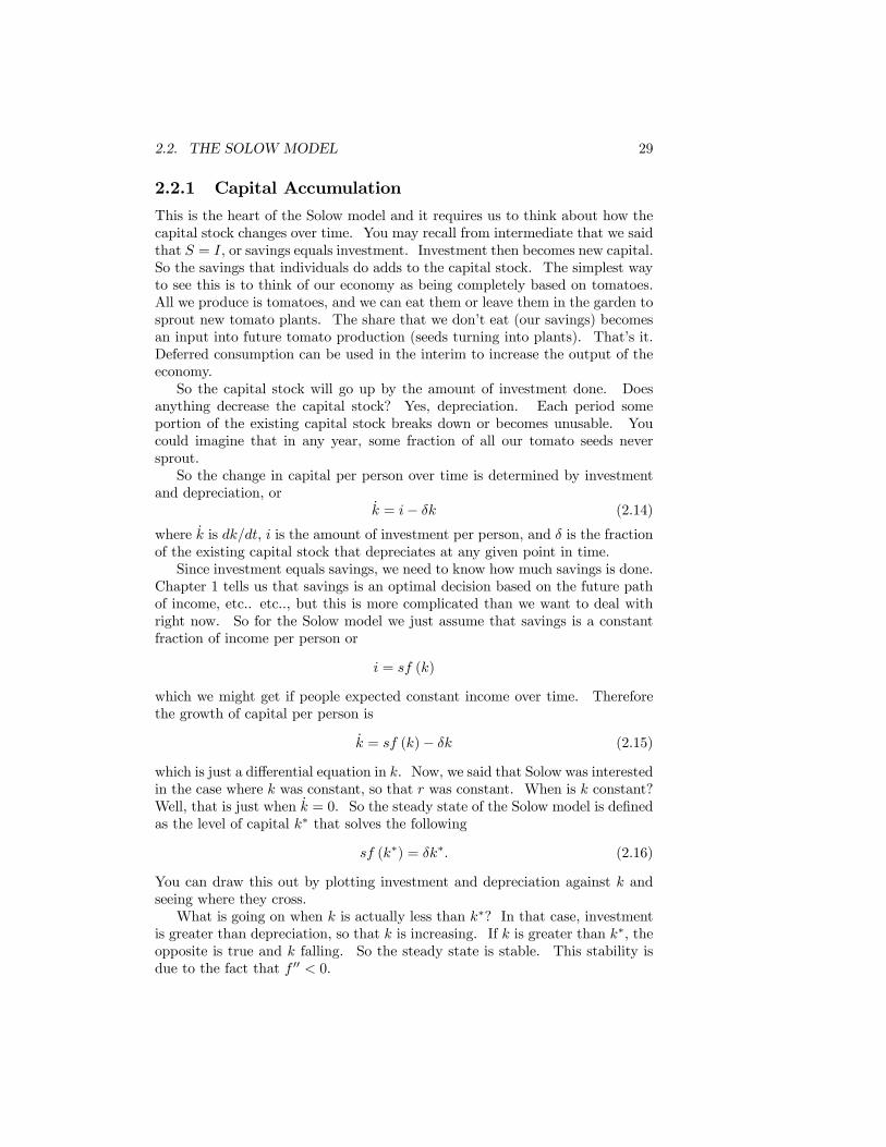
This is the heart of the Solow model and it requires us to think about how thecapital stock changes over time. You may recall from intermediate that we saidthat S = I, or savings equals investment. Investment then becomes new capital.So the savings that individuals do adds to the capital stock. The simplest wayto see this is to think of our economy as being completely based on tomatoes.All we produce is tomatoes, and we can eat them or leave them in the garden tosprout new tomato plants. The share that we don’t eat (our savings) becomesan input into future tomato production (seeds turning into plants). That’s it.Deferred consumption can be used in the interim to increase the output of theeconomy.So the capital stock will go up by the amount of investment done. Does
anything decrease the capital stock? Yes, depreciation. Each period someportion of the existing capital stock breaks down or becomes unusable. Youcould imagine that in any year, some fraction of all our tomato seeds neversprout.So the change in capital per person over time is determined by investment
and depreciation, ork = i− δk (2.14)
where k is dk/dt, i is the amount of investment per person, and δ is the fractionof the existing capital stock that depreciates at any given point in time.Since investment equals savings, we need to know how much savings is done.
Chapter 1 tells us that savings is an optimal decision based on the future pathof income, etc.. etc.., but this is more complicated than we want to deal withright now. So for the Solow model we just assume that savings is a constantfraction of income per person or
i = sf (k)
which we might get if people expected constant income over time. Thereforethe growth of capital per person is
k = sf (k)− δk (2.15)
which is just a differential equation in k. Now, we said that Solow was interestedin the case where k was constant, so that r was constant. When is k constant?Well, that is just when k = 0. So the steady state of the Solow model is definedas the level of capital k∗ that solves the following
sf (k∗) = δk∗. (2.16)
You can draw this out by plotting investment and depreciation against k andseeing where they cross.What is going on when k is actually less than k∗? In that case, investment
is greater than depreciation, so that k is increasing. If k is greater than k∗, theopposite is true and k falling. So the steady state is stable. This stability isdue to the fact that f 00 < 0.
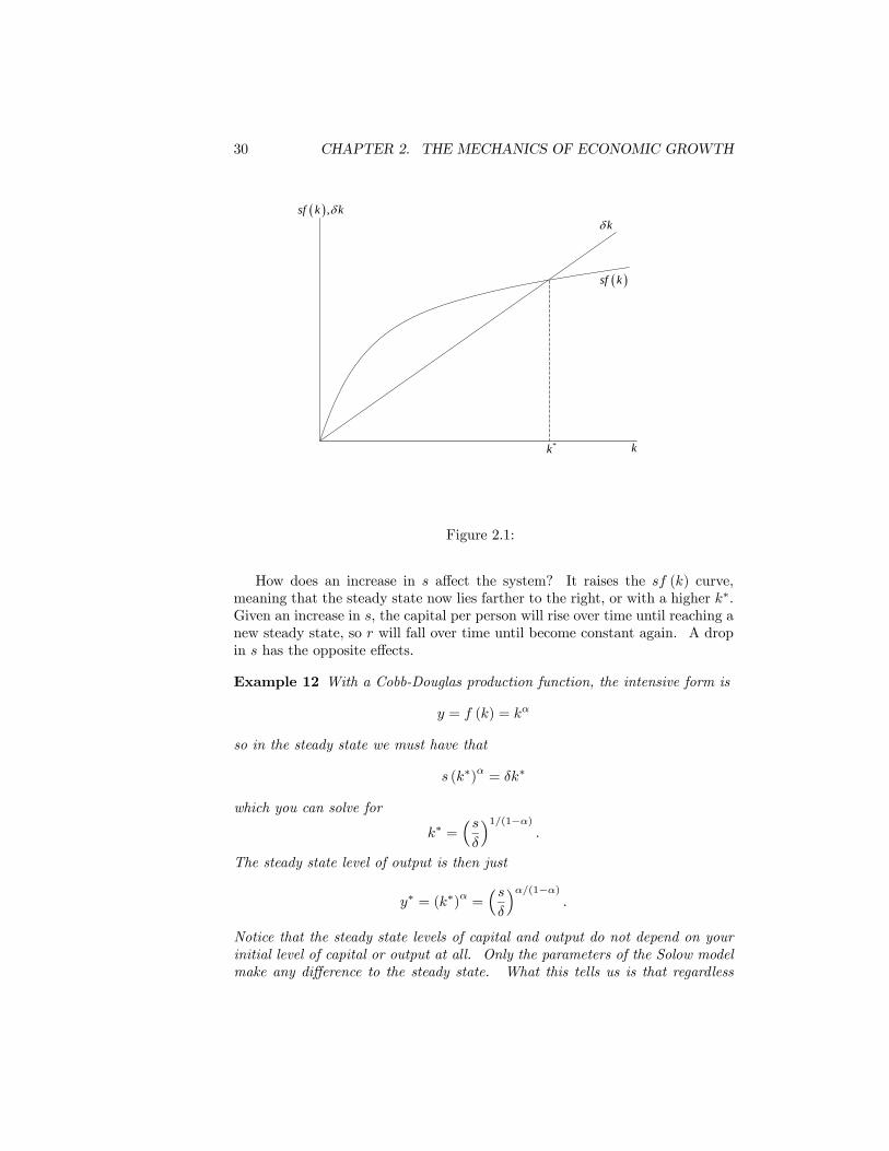
30 CHAPTER 2. THE MECHANICS OF ECONOMIC GROWTH
k
( ) ,sf k kδkδ
( )sf k
*k
Figure 2.1:
How does an increase in s affect the system? It raises the sf (k) curve,meaning that the steady state now lies farther to the right, or with a higher k∗.Given an increase in s, the capital per person will rise over time until reaching anew steady state, so r will fall over time until become constant again. A dropin s has the opposite effects.
Example 12 With a Cobb-Douglas production function, the intensive form is
y = f (k) = kα
so in the steady state we must have that
s (k∗)α = δk∗
which you can solve for
k∗ =³sδ
´1/(1−α).
The steady state level of output is then just
y∗ = (k∗)α =³sδ
´α/(1−α).
Notice that the steady state levels of capital and output do not depend on yourinitial level of capital or output at all. Only the parameters of the Solow modelmake any difference to the steady state. What this tells us is that regardless
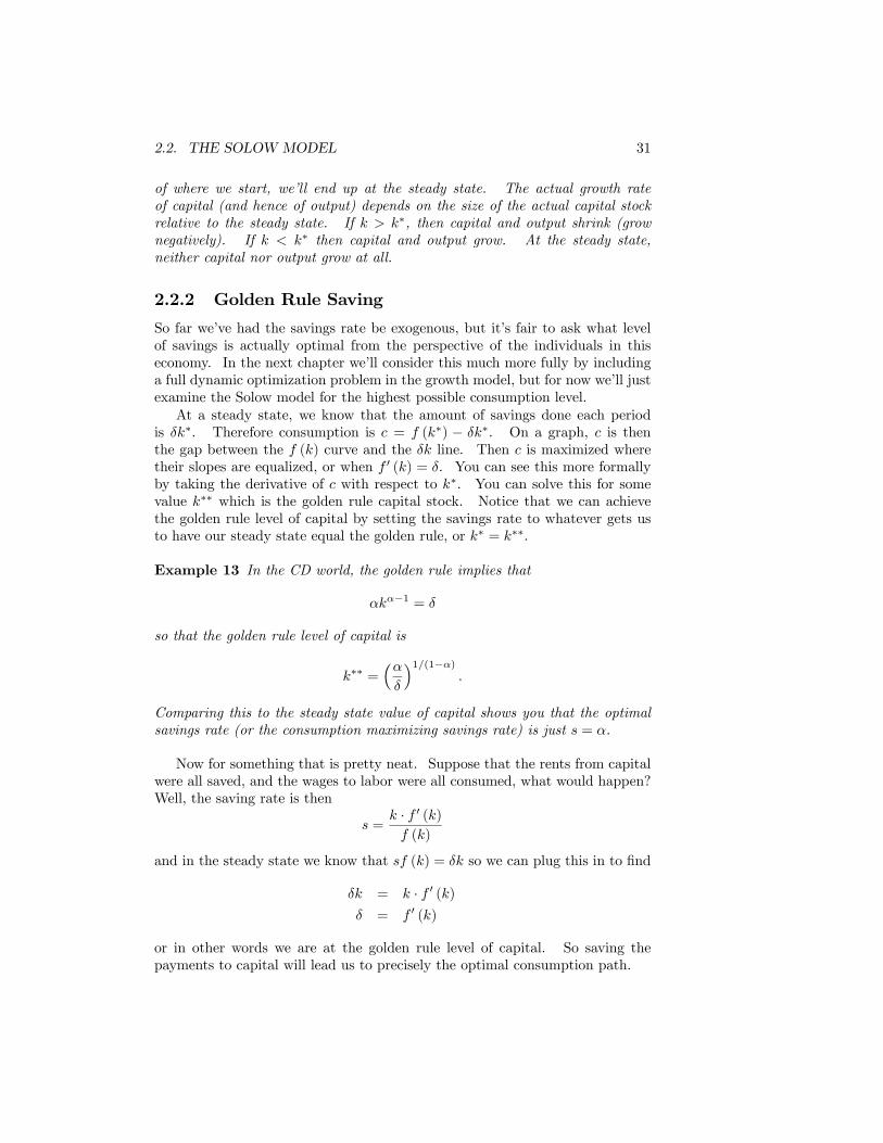
2.2. THE SOLOW MODEL 31
of where we start, we’ll end up at the steady state. The actual growth rateof capital (and hence of output) depends on the size of the actual capital stockrelative to the steady state. If k > k∗, then capital and output shrink (grownegatively). If k < k∗ then capital and output grow. At the steady state,neither capital nor output grow at all.
2.2.2 Golden Rule Saving
So far we’ve had the savings rate be exogenous, but it’s fair to ask what levelof savings is actually optimal from the perspective of the individuals in thiseconomy. In the next chapter we’ll consider this much more fully by includinga full dynamic optimization problem in the growth model, but for now we’ll justexamine the Solow model for the highest possible consumption level.At a steady state, we know that the amount of savings done each period
is δk∗. Therefore consumption is c = f (k∗) − δk∗. On a graph, c is thenthe gap between the f (k) curve and the δk line. Then c is maximized wheretheir slopes are equalized, or when f 0 (k) = δ. You can see this more formallyby taking the derivative of c with respect to k∗. You can solve this for somevalue k∗∗ which is the golden rule capital stock. Notice that we can achievethe golden rule level of capital by setting the savings rate to whatever gets usto have our steady state equal the golden rule, or k∗ = k∗∗.
Example 13 In the CD world, the golden rule implies that
αkα−1 = δ
so that the golden rule level of capital is
k∗∗ =³αδ
´1/(1−α).
Comparing this to the steady state value of capital shows you that the optimalsavings rate (or the consumption maximizing savings rate) is just s = α.
Now for something that is pretty neat. Suppose that the rents from capitalwere all saved, and the wages to labor were all consumed, what would happen?Well, the saving rate is then
s =k · f 0 (k)f (k)
and in the steady state we know that sf (k) = δk so we can plug this in to find
δk = k · f 0 (k)δ = f 0 (k)
or in other words we are at the golden rule level of capital. So saving thepayments to capital will lead us to precisely the optimal consumption path.
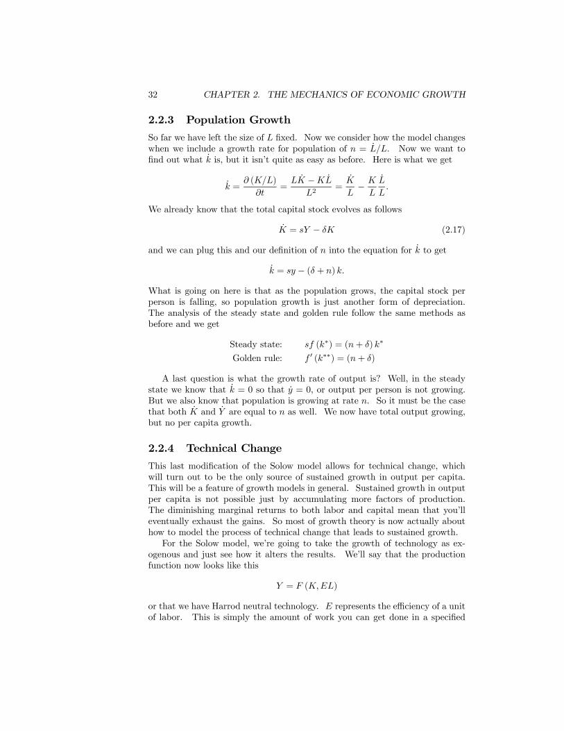
32 CHAPTER 2. THE MECHANICS OF ECONOMIC GROWTH
2.2.3 Population Growth
So far we have left the size of L fixed. Now we consider how the model changeswhen we include a growth rate for population of n = L/L. Now we want tofind out what k is, but it isn’t quite as easy as before. Here is what we get
k =∂ (K/L)
∂t=
LK −KL
L2=
K
L− K
L
L
L.
We already know that the total capital stock evolves as follows
K = sY − δK (2.17)
and we can plug this and our definition of n into the equation for k to get
k = sy − (δ + n) k.
What is going on here is that as the population grows, the capital stock perperson is falling, so population growth is just another form of depreciation.The analysis of the steady state and golden rule follow the same methods asbefore and we get
Steady state: sf (k∗) = (n+ δ) k∗
Golden rule: f 0 (k∗∗) = (n+ δ)
A last question is what the growth rate of output is? Well, in the steadystate we know that k = 0 so that y = 0, or output per person is not growing.But we also know that population is growing at rate n. So it must be the casethat both K and Y are equal to n as well. We now have total output growing,but no per capita growth.
2.2.4 Technical Change
This last modification of the Solow model allows for technical change, whichwill turn out to be the only source of sustained growth in output per capita.This will be a feature of growth models in general. Sustained growth in outputper capita is not possible just by accumulating more factors of production.The diminishing marginal returns to both labor and capital mean that you’lleventually exhaust the gains. So most of growth theory is now actually abouthow to model the process of technical change that leads to sustained growth.For the Solow model, we’re going to take the growth of technology as ex-
ogenous and just see how it alters the results. We’ll say that the productionfunction now looks like this
Y = F (K,EL)
or that we have Harrod neutral technology. E represents the efficiency of a unitof labor. This is simply the amount of work you can get done in a specified
2.2. THE SOLOW MODEL 33
amount of time. As E increases, labor is more productive. More importantlyfor the model, the growth of E is like you are adding new workers to the economy.The growth of E is given by g = E/E. To analyze the Solow model now,
we make a trick of notation and rephrase the intensive forms of the productionfunction by saying that now
k = K/EL
y = Y/EL
which allows us to write the intensive production function as
y = f³k´.
Now let’s analyze the change in k over time, just like before
∂k/∂t =∂K/EL
∂t=
ELK −KEL−KLE
(EL)2
=K
EL− K
EL
L
L− K
EL
E
E.
We know again from (2.17) how to write K and we have definitions for L/L andE/E so we get the following
∂k/∂t = sf³k´− (n+ δ + g) k (2.18)
which says that the capital stock per efficiency unit is subject to two forces.First, savings increases the capital stock, raising the level of capital per efficiencyunit. Second, there is depreciation of the capital stock per efficiency unit, asδ decreases K, n increases L, and g increases E. This makes it sound liketechnology growth is bad, but recall that we are talking about the growth of thecapital stock per efficiency unit, not the capital stock per person. Technologyis making it seem as if there are more people working, but there in reality arenot more people.In the steady state we know that ∂k/∂t = 0, and that ∂y/∂t = 0. What
does this mean for the growth rate of capital and output per worker? Let’slook at the growth of output per worker
∂Y/L
∂t=
∂Y/EL
∂t+
∂E
∂t
= ∂y/∂t+ E/E
= 0 + g
= g.
So we have that output per person is growing at rate g in the steady state whenwe have technology growth. This result follows through for capital per workeras well.
34 CHAPTER 2. THE MECHANICS OF ECONOMIC GROWTH
Now the growth rate of capital per worker or output per worker when we areNOT in the steady state differs from g. How? Well, recall that if we are belowthe steady level of k∗ then k is growing, and therefore y is growing. Lookingat the derivation above, we see that this means that output per person is thengrowing faster than g. The reverse also holds. If k > k∗, then output perperson would be growing slower than g. But the steady state level of growth isalways g.The last thing we might consider is what the actual interest rate or wage
rate is (as this may be useful when we consider individual optimization later).What is the interest rate in the situation with technological change? Recallthat a firm in this economy is trying to maximize profits, which can be writtenas follows
π = F (K,EL)− (r + δ)K − wL
where r+ δ is the total rate that a firm has to pay for capital services. We canconsider a firm with an arbitrary size, where size is measured as the number ofeffective units of labor employed. Now profits are
π = ELnf³k´− (r + δ) K − wE
owhich can be maximized, given r and w, to get the following
f 0³k´− δ = rh
f³k´− kf 0
³k´i
E = w.
This shows that the interest rate in a model with constant technological progressis constant. The wage rate, though, grows as E grows.
2.3 Human CapitalThe dynamics of the Solow model come from the accumulation of capital. Wegenerally think of capital as machines and buildings, but there are other formsof capital we want to expand out thinking to include.. Namely, human capital.We’re going to add a new factor of production to our analysis that can beaccumulated as well.The way we’ll do this makes human capital operate just like physical capital
(it accumulates through savings and depreciates, etc..) which may not be exactlyrealistic. But the mechanics of how H will evolve allow us to see how a secondaccumulable factor changes the results of the Solow model. We won’t be ableto go into, in this course, other modifications we can make to the model to makehuman capital more realistic. This generally involves making the decision toobtain it endogenous.So first we write our overall production function as follows
Y = KαHβ (EL)1−α−β (2.19)
2.3. HUMAN CAPITAL 35
where H is the human capital stock at any given point in time. We’ll doeverything in per efficiency units (so that h = H/EL) and we get
y = kαhβ
and this intensive function looks a lot like the ones with only capital. Inparticular, it has the property that this intensive form of the production functionis decreasing returns to scale. That is, if I doubled both k and h, I’d get lessthan 2 times the output. This property ensures that we’ll have both k and hequal to zero in the steady state (we can’t generate output fast enough to keepboth stocks growing). We assume that H is accumulated in a pattern just likethat of K, with it’s own savings rate so that we have
k = sky − (n+ δ + g) k
h = shy − (n+ δ + g)h
To find the steady state you set both of these to zero and solve together to find
k∗ =
Ãs1−βk sβhn+ δ + g
!1/(1−α−β)
h∗ =
µsαks
1−αh
n+ δ + g
¶1/(1−α−β)which you’ll notice are very similar and have a form related to the k only steadystate. What does this model tell us is happening to k and h in the steadystate? They both are growing at the rate zero. So their ratio must be stayingconstant, or k/h is fixed in the steady state. What is this ratio? You can solveit out to see that
k∗
h∗=
sksh
or their ratio just depends on the relative savings rates. But notice that thisimplies that the ratio of K/H must be constant as well, or the overall stocksof physical and human capital must both be growing at the same rate of n+ g.This holds even though there are different savings rates.The addition of another type of capital doesn’t change the overall implica-
tions of the Solow model. Increases in savings rates or decreases in populationgrowth rates both increase income. Exogenous changes in the capital stockscreate changes in the growth rate of income based on whether you are aboveor below steady states. The additional factor to consider is that k and h bearsome relationship to each other, and so a change in one will alter the growthrate of the other.

36 CHAPTER 2. THE MECHANICS OF ECONOMIC GROWTH
Chapter 3
Essential Models ofDynamic Optimization
Whether you believe it or not, you now have all the intution necessary to un-derstand the full blown models of dynamic optimization that sit at the heart ofalmost every macroeconomic paper written today or in the last twenty years.The two models are the infinitely lived agent model and the overlapping genera-tions model. This chapter is going to cover the mathematics of these models insome detail, as I want you to see how the discrete and continuous time modelsmimic each other. I also want to show how there are different mathematicalmethods of looking at these problems, but that ultimately the methods are allgetting the same answers.This analysis is fundamentally identical to the two period models we looked
at so far, but simply extends the analysis out to T periods of life. Friedmananticipated all of this, but at the time of his writing the mathematics was notavailable to solve the problems he had in mind. It’s important to rememberthat we should be impressed with Friedman’s insight, not with the fancy math.
3.1 The T Period Fisher Model
The Fisher model easily extends to multiple periods. The person is now plan-ning consumption over periods 0 to T − 1, (which are labelled this way forconvenience). The path of wages is W0...WT−1. The person gets utility fromthe felicity function of U (Ct) which is discounted at rate θ. So utility is
V =T−1Xt=0
U (Ct)
(1 + θ)t(3.1)
The interest rate is r, is constant over time, and the person can borrow orsave at this rate. Call At the assets the person has at the beginning of a period,
37
38 CHAPTER 3. ESSENTIAL MODELS OF DYNAMIC OPTIMIZATION
thenAt = (1 + r) ∗ (At−1 +Wt−1 − Ct−1) (3.2)
and the person starts with A0 = 0. We also impose that the person must havezero assets at the end of life, or AT = 0. In other words, in period T − 1 theperson consumes everything they have left, and they cannot die in debt.We can use this information to get the intertemporal budget constraint.
Note that
A1 = (1 + r) (W0 − C0)
A2 = (1 + r) (A1 +W1 − C1) = (1 + r) (W1 − C1) + (1 + r)2 (W0 − C0)
· · ·AT = (1 + r) (WT−1 − CT−1) + (1 + r)2 (WT−2 − CT−2) +
. . .+ (1 + r)T (W0 − C0)
Divide all the terms in AT by (1 + r)T and note that because AT = 0 wecan write
0 =T−1Xt=0
Wt − Ct
(1 + r)t(3.3)
and notice that all the asset terms are gone. Rearrange this slightly and wecan see that
T−1Xt=0
Wt
(1 + r)t =
T−1Xt=0
Ct
(1 + r)t (3.4)
which says that the present discounted value of wages has to be equal tothe present discounted value of consumption. This is identical to the 2 periodbudget constraint, just extended to T periods.Given both (3.1) and (3.3) we can set up a massive Lagrangian like this
L =T−1Xt=0
U (Ct)
(1 + θ)t− λ
T−1Xt=0
Wt − Ct
(1 + r)t(3.5)
and to solve this we’d have T +1 first order conditions which we could solvetogether for λ and the T values of Ct. However, this is a mess, and we can getpretty far by just looking at the FOC of two adjacent periods, t and t+ 1.
∂L
∂Ct=
U 0 (Ct)
(1 + θ)t− λ
1
(1 + r)t= 0 (3.6)
∂L
∂Ct+1=
U 0 (Ct+1)
(1 + θ)t+1− λ
1
(1 + r)t+1= 0 (3.7)
which can be combined to give the following
U 0 (Ct)
U 0 (Ct+1)=1 + r
1 + θ(3.8)
3.1. THE T PERIOD FISHER MODEL 39
which relates consumption in adjacent periods. Notice that just like in the2 period Fisher problem, this condition doesn’t depend on total income. Thecondition in (3.8) is of central importance to all models of dynamic optimization,and is referred to as an Euler equation. It doesn’t allow us to understand thelevel of Ct or Ct+1, only their relative size.To see the centrality of this result, let’s think through this without doing
the math. I have some set of total consumption I’d like to do, how will I divideit up between multiple periods? Let’s take any given path of consumption Icould choose (C0...CT−1). Is this path optimal? Let’s perturb this path andsee what I get. So let’s imagine I consume one less unit in period zero, save itand then consume the 1 + r extra units in period 1.What would I lose? I would lose U 0 (C0) of utility. (We assume the one
unit of consumption is small relative to C0).What would I gain? I would get an additional 1 + r units of consumption
in period 1, and this would give me (1 + r)U 0 (C1) in utility, but I have toremember to discount this, so my total gain is β (1 + r)U 0 (C1).Now, if these are not equal to each other, then I could gain in total utility
by moving one unit of consumption around. So if my path (C0...CT−1) isoptimal, then it must be the case that β (1 + r)U 0 (C1) = U 0 (C0), and a similarlogic must hold between any other two periods as well. This is just the Eulerequation we got from (3.8).So let’s look at the Euler equation some more and see what it is telling us
about how consumption changes over time. What happens if r > θ, so thatU 0(Ct)U 0(Ct+1)
< 1. This means that marginal utility in period t must be greater thanin period t+1, and this implies that Ct < Ct+1. So if r > θ, it must be the casethat consumption is rising over time. The return on savings is so high that itis worth having low initial consumption, saving a lot, and then consuming a lotin the future.On the other hand, if r < θ, the opposite holds and Ct > Ct+1, or consump-
tion is falling over time. The return on savings is so low that it isn’t worthforgoing consumption today. I prefer to consume as much as I can right now,and over time my consumption will decrease.If r = θ then these two effects exactly balance out, and I want to consume
the same exact amount in every period. Recall that this holds regardless of theactual path of my income.Note that the speed with which consumption grows or shrinks over time
depends on the actual form of the marginal utility. And the form of marginalutility is summarized by the measure of risk aversion. The more risk averse Iam, the more concerned I am with having smooth consumption (even in everyperiod). So if I am very risk averse, it will take a really big gap or r > θ forme to choose to have a steeply increasing consumption path. If I am close torisk neutral, then I’m very sensitive to any difference between the interest rateand discount rate.To see this, consider the CRRA utility function, which has a marginal utility
40 CHAPTER 3. ESSENTIAL MODELS OF DYNAMIC OPTIMIZATION
of U 0 (Ct) = C−σt . Putting this in the Euler equation gives us
Ct+1
Ct=
µ1 + r
1 + θ
¶1/σ(3.9)
and we have an expression for exactly the relative size of consumption in adjacentperiods. The larger σ, the closer this ratio goes to one. So the more risk averseyou are, the closer your consumption path is to equal consumption in everyperiod.
3.1.1 Infinitely Lived Agents
This will be quick, because it is nothing more than the Fisher T period problemextended to T =∞. The problem is then as follows
max∞Xt=0
U (ct)
(1 + θ)t(3.10)
subject to
at+1 = (at + wt − ct) (1 + r) (3.11)
where at are assets at time t, wt is your income at time t, and r is fixed overall periods. Again we assume that a0 = a0, a fixed amount that could be zero.To rule out the possibility that people have infinite consumption financed byinfinite borrowing, we impose the following present value budget constraint
a0 +∞Xt=0
wt
(1 + r)t =
∞Xt=0
ct
(1 + r)t (3.12)
You can set up a Lagrangian again, get the FOC for two adjacent periods,solve them together and get the Euler equation that says
U 0 (ct)
U 0 (ct+1)=1 + r
1 + θ(3.13)
and this has the same interpetation as in the multiple period Fisher model.Given the FOC, we could conceivably solve this explicitly for a value of c0
that satisfied the budget constraint as well. Without further specifications forthe utility function, though, we don’t have enough information. A lot of thetime it will be enough to understand the Euler equation.
Example 14 But let’s not leave it at that. If we have CRRA utility, whatcan we say about the optimal consumption path? First, we know that our Eulerequation implies that
ct+1ct
=
µ1 + r
1 + θ
¶1/σ
3.1. THE T PERIOD FISHER MODEL 41
and we can use this to tell us something about c0 and c1. Specifically,
c1 =
µ1 + r
1 + θ
¶1/σc0
and by analogy
c2 =
µ1 + r
1 + θ
¶1/σc1 =
µ1 + r
1 + θ
¶1/σ µ1 + r
1 + θ
¶1/σc0
or
c2 =
"µ1 + r
1 + θ
¶1/σ#2c0
which we can logically then extend to
ct =
"µ1 + r
1 + θ
¶1/σ#tc0
Now, we can use this last equality to plug into our intertemporal budget con-straint from (3.12) to give us
a0 +∞Xt=0
wt
(1 + r)t=∞Xt=0
"µ1 + r
1 + θ
¶1/σ#tc0
1
(1 + r)t
which can be rewritten as
a0 +∞Xt=0
wt
(1 + r)t = c0
∞Xt=0
"(1 + r)
1/σ−1
(1 + θ)1/σ
#tFor the summation on the right to converge, we need that
(1 + r)1/σ−1
(1 + θ)1/σ< 1
or that(1 + r)
1−σ< 1 + θ
which tells us that to even have an answer, we have to have a discount rate that is"large enough". Large enough to what? Large enough to keep me from wantingto save too much and end up with infinite consumption later in life. Noticethat an increase in σ means that the left hand side goes towards zero. Thismeans that you can have a smaller discount rate and still get a solution. Why?Because as sigma rises, this means that people prefer flat consumption, and areless likely to choose explosive consumption growth. Regardless, assuming thatthe above condition holds, we can get an answer for c0 that looks like this
c0 =
"(1 + r) (1 + θ)1/σ − (1 + r)1/σ
(1 + r) (1 + θ)1/σ
#"a0 +
∞Xt=0
wt
(1 + r)t
#
42 CHAPTER 3. ESSENTIAL MODELS OF DYNAMIC OPTIMIZATION
and notice that the first term in this just defines a fraction between 0 and 1.What this says is that the interest rate, discount rate and coefficient of riskaversion determine what share of your total PDV of income that you consumein period zero. You can have some fun figuring out the derivatives of c0 withrespect to the different parameters. To see some simple logic, assume we havelog utility, so that σ = 1. This gives us
c0 =
∙θ
1 + θ
¸"a0 +
∞Xt=0
wt
(1 + r)t
#
and the interest rate falls out. The higher the discount rate, the higher theinitial consumption, as expected.
3.1.2 Dynamic Programming
Dynamic programming is a method of writing and solving dynamic optimizationproblems that differs from the Lagrangian. It uses recursive equations, alsocalled Bellman equations, to break a T period problem up into a bunch of muchsmaller one period problems. The most important thing to note is that theproblem itself is not any different, only the solution method has changed. So westill have individuals trying to maximize their lifetime utility subject to someconstraints on their lifetime wages and assets. We should get out exactly thesame Euler equation.If you read a book like Stokey and Lucas (1989), or Sargent (1987), much
of the text is spent proving to you that it is theoretically possible to solve thefollowing problem
maxc1..c∞
V =∞Xt=0
U (ct)
(1 + θ)t(3.14)
subject to
at+1 = (at + wt − ct) (1 + r) (3.15)
by using the techniques of dynamic programming. We’ll take that proof as agiven, and just proceed to show you how the method actually works. The proofdepends a lot on the presence of time-separable preferences and then requiresU(c) to be concave, continuous, etc..The first step is to write down the value function, which in these problems
you can think of as being similar to an indirect utility function.
Vt (at) = maxct
∞Xs=t
U (cs)
(1 + θ)s s.t. at+1 = (at + wt − ct) (1 + r) (3.16)
This value function tells us that V is the maximized value of utility I have,given an initial asset level of at, from time period t until infinity, along my
3.1. THE T PERIOD FISHER MODEL 43
optimal path. Bellman then used the insight that if you performed your op-timization at time t+1, the path of consumption that you would choose mustfollow the exact same path that you would have chosen for periods t+1 to in-finity if you had done your optimization at time t. (The crucial assumption forthis is that preferences are time separable).This means I can write the above value function recursively, or as follows:
Vt (at) = maxct
½U (Ct) +
Vt+1 (at+1)
1 + θ
¾s.t. at+1 = (at + wt − ct) (1 + r)
(3.17)This recursive, or Bellman, equation tells us that the value of my lifetime
utility from time t forward is equal to the utility of consumption at time t plusthe value of my lifetime utility from time t+1 forward.Suppose for the moment that I actually know what the V function looks
like (and notice that the V function can possibly change over time). Then myproblem is no longer a many period problem but only a one period problem.The question is trading off current utility at time t for more financial wealth attime t+1 (which I already know I will spread optimally among the remainingperiods of my life).So let’s do the maximization in the Bellman equation. This gives us the first
order condition that
U 0 (Ct) =1
1 + θ
©(1 + r)V 0
t+1 (at+1)ª
(3.18)
which is already starting to look a lot like the Euler equation we foundbefore. This says that I should trade off the marginal utility of consumptiontoday against the (suitably discounted) marginal value of remaining lifetimeutility starting tomorrow. But we don’t know what this V function looks like,so this equation doesn’t help us a lot.However, the next big insight in the dynamic programming method is that
there is a simple envelope relationship between V’ and U’ along the optimalpath.1 That is, the derivative of V with respect to assets is just
V 0t+1 (at+1) =
1
1 + θ(1 + r)V 0
t+2 (at+2) . (3.19)
But we know that since V’ in t+1 is the maximized value of utility, thenit must be the case from the t+1 FOC that the right hand side of the aboveequation is equal to the marginal utility of consumption in period t+1. Thismeans that
V 0t+1 (at+1) = U 0 (Ct+1) .
1More formally, the envelope theorem says that if you have y=max f(x,c) w.r.t x, then thederivative dy/dc can be evaluated as follows. First, define x*=g(c) as the optimal value of xgiven a value of c. Write y=f(g(c),c). Now dy/dc = f1(g(c),c)g’(c)+f2(g(c),c). But we knowthat f1(g(c),c)=0 by the first order conditions that made x*=g(c) in the first place. So thefirst term drops out and dy/dc = f2(g(c),c). In other words, the derivative of y with respectto c is just the derivative of the original f(x,c) function with respect to c.
44 CHAPTER 3. ESSENTIAL MODELS OF DYNAMIC OPTIMIZATION
Plugging this into the original period t FOC gives us
U 0 (Ct) =1
1 + θ{(1 + r)U 0 (Ct+1)} (3.20)
and this is obviously just the Euler equation.Solving the model completely requires that you then solve the Euler equation
for some consumption path and utilize the budget constraint. This is just thesame as before. The dynamic programming method doesn’t necessarily offer anyextra help during these last steps. It’s main value is that certain problems areeasier to set up as Bellman equations in the first place. The recursive equationsare also useful because they are easier to translate to computer code that caniterate through periods quickly to find the optimal path (which allows you tocalibrate your model).An additional mathematical result of this technique that can be useful in-
volves the nature of V. Under a certain set of conditions (continuity, concavity,etc..) it can be shown that the Bellman equation is an example of a contractionmapping, and that this means the V functions (which were previously allowedto vary over time) will converge to a single functional form V (at). In addition,this means that the control function, or the rule for setting consumption in timet as a function of assets at time t, will be time invariant as well.
Example 15 To see what this means, consider a problem with log utility, sothat
Ct+1 =1 + r
1 + θCt
and therefore consumption in any period s>t can be written as
Cs =
µ1 + r
1 + θ
¶sCt.
The budget constraint at time t is the following
∞Xs=t
Cs
(1 + r)s−t= At +
∞Xs=t
Ws
(1 + r)s−t
And you can solve these together to get that
Ct =θ
1 + θ
"At +
∞Xs=t
Ws
(1 + r)s−t
#.
This rule holds for any period t, so the consumption rule (or control rule) isidentical for all periods. This doesn’t mean that consumption itself is neces-sarily identical every period, but the rule for setting it is. You may still haveconsumption rising or falling depending on the relationship of r and the discountrate.
3.1. THE T PERIOD FISHER MODEL 45
3.1.3 Lifespan Uncertainly and Insurance
I can set this up more generally in a T period problem by assuming that I havea Pt chance of being alive in period t. Then my expected utility in my life is
EV =T−1Xt=0
PtU (Ct)
(1 + θ)t(3.21)
and I have a similar budget constraint to the regular T period problem. Notethat the budget constraint describes how my assets are related to wages andconsumption assuming that I am alive. The only uncertainty in the model iswhen you die, and since when that happens you can’t change anything, youmight as well plan out your whole path of consumption from the beginning. Nonew information arises during your life that you can actually use.We still hold that you cannot die with negative assets, so this means you
have to have positive assets in every period. There is some unpleasant mathinvolving this, but we can get around it by assuming we have someone with onlyan initial stock of wealth but no wage income. The Lagrangian looks like this
L =T−1Xt=0
PtU (Ct)
(1 + θ)t+ λ
ÃA0 −
T−1Xt=0
Ct
(1 + r)t
!(3.22)
and we get FOC from periods t and t+ 1 that show
U 0 (Ct+1)
U 0 (Ct)=1 + θ
1 + r
PtPt+1
(3.23)
and now we have some fun with math. First we’ll rewrite the ratio of dyingprobabilities as
PtPt+1
=Pt+1 + (Pt − Pt+1)
Pt+1= 1 +
(Pt − Pt+1)
Pt+1≈ 1 + ρt
where ρt is the probability of dying in a given period conditional on having livedto that age in the first place. The Euler equation is then
U 0 (Ct+1)
U 0 (Ct)=1 + θ
1 + r(1 + ρt) ≈
1 + θ + ρt1 + r
which shows us that we’ve basically just modified the discount rate (by raisingit) so that we’ll get a consumption path tilted more towards current periodconsumption.Now the individual in this problem will always die holding onto some assets
unless she happens to get very lucky and live all the way to period T . Leavingassets on the table doesn’t help her consumption very much, so could we makeher better off? Yes, buy getting her an annuity.So if we have a constant probability of dying each period, ρt = ρ for all t,
and some market interest rate of r, we could start a company that makes deal
46 CHAPTER 3. ESSENTIAL MODELS OF DYNAMIC OPTIMIZATION
with each individual that says "Give me your assets, and I will pay you somerate of interest z, but if you die before next year I get to keep all the assetsremaining." Now obviously z has to be above r, or the individuals wouldn’ttake the deal. So what should z be? Well, assume that the annuity market iscompetitive, so that there are no profits to be made. Then it must be that myannuity company equates
(1 + z) (1− ρ) = (1 + r) (3.24)
which says that the amount I have to pay out to individuals is (1 + z) (1− ρ):I pay the rate z to everyone who is still alive, which happens with probability1−ρ. The amount I earn on the assets I’m holding from these people is (1 + r).I can solve this out to see that
z = (1 + r) / (1− p)− 1 ≈ (1 + r + ρ)− 1 = r + ρ
Now the individuals have a new interest rate of z that they earn each period,so their Euler equation is
U 0 (Ct+1)
U 0 (Ct)=1 + θ + ρ
1 + z=1 + θ + ρ
1 + r + ρ.
What this tells us is that if r = θ, the person will still have flat consumptionacross periods, even though her probability of being dead was rising. We’vegotten the person around the problem of having to have declining consumptionin the face of death by paying her a higher interest rate than she otherwisewould face. And that is how annuities generally work. You trade your lumpsum of assets for a predictable stream of income, with the insurance companyoffering to pay you a higher rate of return in exchange for the chance to keepyour money if you die.
3.1.4 Continuous Time Optimal Consumption
We can reconsider the whole question of dynamic optimization, except now wecan look at a continuous time version. That is, people don’t have discreteperiods of life, but evolve, well, continuously. This is primarily just a changein notation and mathematical technique, but all the same intuitions still apply.Now we have
maxc
Z ∞0
e−θtU (c) dt (3.25)
subject to the constraint that
a = ra+ w − c (3.26)
where a is now the instantaneous level of assets, w is the instantaneous wagerate, c is the instantaneous level of consumption, and r is the constant rate ofinterest. In the utility function, θ again represents the discount rate, only it isset up in continuous time. The level of a is the state variable, meaning that
3.1. THE T PERIOD FISHER MODEL 47
it does not jump around, while c is the control variable, meaning that it can.2 .For all variables, I’ve dropped the time subscript for convenience.We again want to eliminate the possibility of unlimited borrowing and infi-
nite consumption, so we have the present value budget constraint of
a0 +
Z ∞0
e−rtwdt =
Z ∞0
e−rtcdt (3.27)
You could set up a Lagrangian, but this is a pain and some Russians in the1950’s found a much better way to go about this. We’ll set up a Hamiltonian,which is written as
H = maxc
©e−θtU (c) + μ (ra+ w − c)
ª(3.28)
which looks a lot like a Lagrangian. However, the multiplier μ is the instanta-neous shadow value of assets, and is time varying. Now, to solve this problemyou need to apply several conditions to the Hamiltonian.3
First, you maximize H with respect to c, as written
U 0 (c) e−θt − μ = 0 (3.29)
and this gives you something that looks like the FOC from the Lagrangian.It’s telling us that we have to balance out the marginal gain in utility fromconsumption against the marginal cost, which is given by μ and represents theshadow value of assets at any given point in time.Next, you recover the constraint by taking ∂H/∂μ = a or
a = ra+ w − c (3.30)
which is just ensuring that we meet the constraint on how assets accumulate.The rate of change of the shadow value of assets, μ = −∂H/∂a or
μ = −μr (3.31)
and this is the least obvious one. The insight of the people who invented thistechnique was proving that this condition held. Finally, we have a transversal-ity condition, which keeps the problem from "blowing up" and having infiniteconsumption later in life. This condition is that
limt→∞
μa = 0 (3.32)
You solve (3.29) , (3.30), and (3.31) together in order to find the solution.First, take (3.29) and take the derivative with respect to time
cU 00 (c) e−θt − θU 0 (c) e−θt − μ = 0
2A state variable is like your weight, while a control variable is like your calorie intake forthe day. You can vary your calorie intake daily, jumping from 100 to 1000 to 5000 caloriesor back. But your weight will only adjust slowly in reaction to changes in the control.
3 I’m not going to cover the theory of optimal control, only utilize the results. You can seeChiang’s book for an explanation of why this all works.
48 CHAPTER 3. ESSENTIAL MODELS OF DYNAMIC OPTIMIZATION
which gives us another expression for μ. Plug (3.31) into the above equationto get
cU 00 (c) e−θt − θU 0 (c) e−θt = −μrNow notice from (3.29) that μ = U 0 (c) e−θt and plug that in to get
cU 00 (c) e−θt − θU 0 (c) e−θt = −U 0 (c) e−θtrStart going crazy with the algebra and you can get the following statement
c
c= (r − θ)
U 0 (c)
cU 00 (c)(3.33)
which describes the growth of consumption over time. Assume for the momentthat the U 0(c)
cU 00(c) term is constant. Then whether consumption is growing orfalling depends on the relative size of r and θ, or exactly what we saw in theFisher model. If r is larger, then consumption is rising as people save theirincomes, and if θ is larger then consumption is falling as people discount thefuture a lot.The second term on the right hand side of (3.33) should be familiar. It’s just
the inverse of the coefficient of relative risk aversion. What it says is that yourconsumption growth will be slower if your risk aversion (smoothing preference)is higher.
Example 16 In the CRRA case, we know exactly what the risk aversion is, σ.So that means that if preferenes are CRRA, the optimal consumption growth is
c
c= (r − θ)
1
σ
Again, solving explicitly for the level of consumption is possible. Equation (3.33)is a first order differential equation with a simple form and has the solution that
ct = c0e1σ (r−θ)t
which gives us a nice way to describe consumption in any period. Now we needthe budget constraint, which was
a0 +
Z ∞0
e−rtwdt =
Z ∞0
e−rtcdt
and we can plug in our formula for ct, play with some algebra and get
a0 +
Z ∞0
e−rtwdt = c0
Z ∞0
e1σ (r(1−σ)−θ)tdt
The integral on the right hand side can be evaluated to be a positive, finitenumber if
(1− σ) r < θ
which is just like the condition we saw in discrete time. Now, evaluating theintegral and rearranging we get that
c0 =1
σ(θ − (1− σ) r)
∙a0 +
Z ∞0
e−rtwdt
¸
3.1. THE T PERIOD FISHER MODEL 49
3.1.5 The Ramsey Model
At this point you may be wondering exactly why we bothered to go over thegrowth material in Chapter 2. We’ll address that concern right now. Whatwe’re going to do, essentially, is make the interest rate endogenous. The opti-mizing agent will know how interest rates are formed, so will take into accountthe effect of their actions on the interest rate in the future. The interest rate issimply the marginal product of capital, so we’ll need to know the capital stock.The capital stock is just accumulated investment effort, which in turn dependson savings. So the savings decisions of individuals lead to the interest rateitself, which of course influences the savings decision in the first place.So let’s think about the agent doing the optimizing. This person is per-
forming the identical problem from the previous section, only now they have toaccount for the fact that now their state variable is k, and it evolves accordingto
k = f (k)− c− nk (3.34)
where I’ve assumed that depreciation and technological growth are both zero tobegin with. This is almost identical to the asset evolution equation in (3.26).In fact, if we assert that each person has one unit of labor to offer at any point,then we can divide up total output as
f (k) = k · f 0 (k) + w
which we established in equation (2.10) in the growth chapter. Putting thisinto the budget constraint gives us
k = k · f 0 (k) + w − c− nk
= k (f 0 (k)− n) + w − c
and this tells us that the effective interest rate for the agent is f 0 (k)− n.So the optimization problem is the same.4 We know how to do the Hamil-
tonian, which gives us the Euler equation. Assuming CRRA utility for simplic-ity, we know that
c
c=1
σ(f 0 (k)− n− θ) (3.35)
So the instantaneous growth rate of consumption depends on the interest rateat that moment. This depends in turn on the actual capital stock at thatmoment. Well, we know how the capital stock evolves over time from (3.34).So we have two differential equations in two unknowns, c and k. We can solvethem together to try and find the steady state where both c and k are constant.We’ll do this by looking at a phase diagram that graphs c against k. We first
think about all the points at which c = 0. This holds only when f 0 (k) = n+ θ,
4Well, not quite. What we are assuming is that the maximization is over the utility ofthe average person in the future. That is, c is consumption per person. An alternativewould be to modify the optimization to be over the total utility of the future generations, orV = ∞
0 U (c) e(n−θ)tdt. Assuming that n < θ, this is just like modifying the discount rate.If n > θ this becomes a matematical nightmare, so we’ll ignore it.
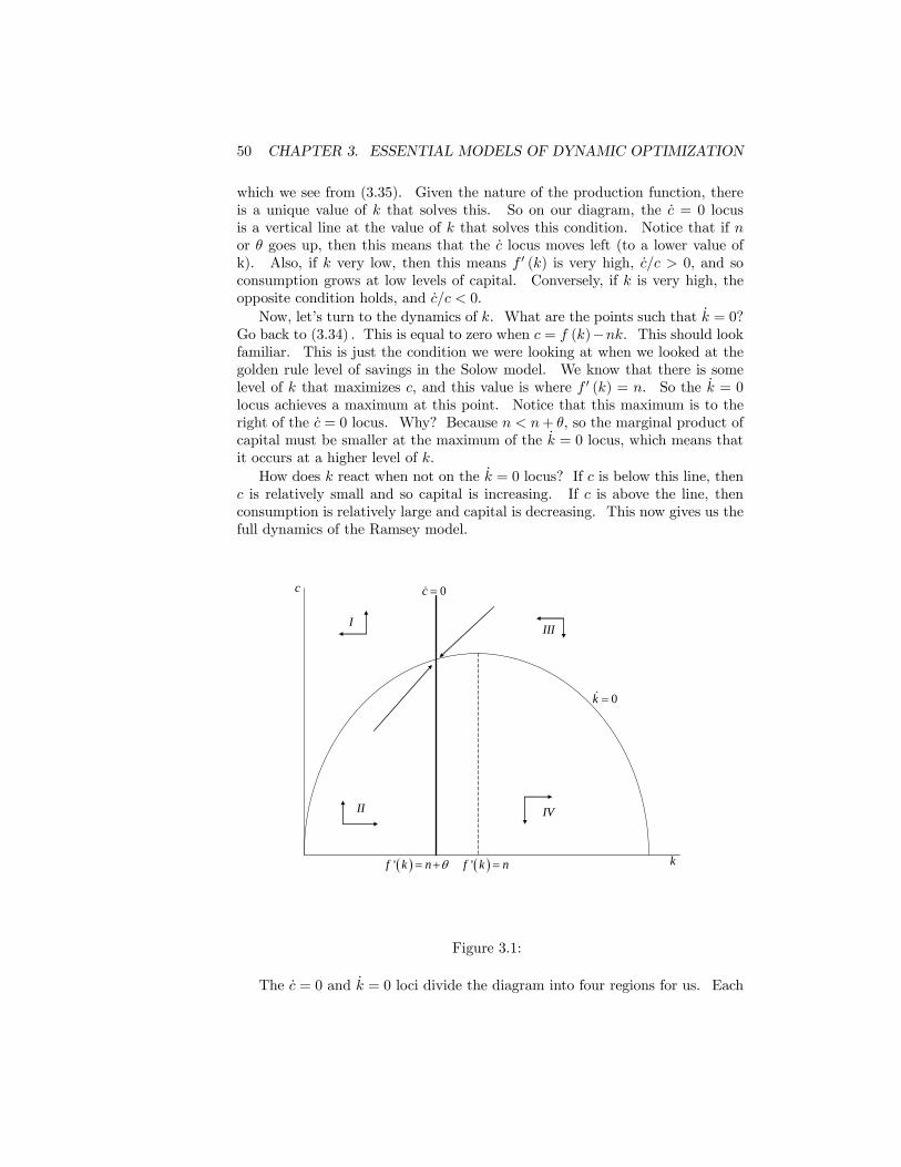
50 CHAPTER 3. ESSENTIAL MODELS OF DYNAMIC OPTIMIZATION
which we see from (3.35). Given the nature of the production function, thereis a unique value of k that solves this. So on our diagram, the c = 0 locusis a vertical line at the value of k that solves this condition. Notice that if nor θ goes up, then this means that the c locus moves left (to a lower value ofk). Also, if k very low, then this means f 0 (k) is very high, c/c > 0, and soconsumption grows at low levels of capital. Conversely, if k is very high, theopposite condition holds, and c/c < 0.Now, let’s turn to the dynamics of k. What are the points such that k = 0?
Go back to (3.34) . This is equal to zero when c = f (k)−nk. This should lookfamiliar. This is just the condition we were looking at when we looked at thegolden rule level of savings in the Solow model. We know that there is somelevel of k that maximizes c, and this value is where f 0 (k) = n. So the k = 0locus achieves a maximum at this point. Notice that this maximum is to theright of the c = 0 locus. Why? Because n < n+ θ, so the marginal product ofcapital must be smaller at the maximum of the k = 0 locus, which means thatit occurs at a higher level of k.How does k react when not on the k = 0 locus? If c is below this line, then
c is relatively small and so capital is increasing. If c is above the line, thenconsumption is relatively large and capital is decreasing. This now gives us thefull dynamics of the Ramsey model.
k
c
( )'f k n θ= +
0c =&
0k =&
I
II
III
IV
( )'f k n=
Figure 3.1:
The c = 0 and k = 0 loci divide the diagram into four regions for us. Each
3.1. THE T PERIOD FISHER MODEL 51
one has different implied dynamics for c and k. In area 1, c is increasing but k isdecreasing. People are essentially eating up their assets and not saving enoughto sustain the capital stock. So any point in area 1 is not feasible because itimplies that consumption increases forever.Area 2 has both increasing consumption and increasing capital, meaning
people are saving enough to increase the capital stock and increase their con-sumption in the future. Points in this area are feasible to sustain, and noticethat they tend to point you towards the point where c = 0 and k = 0 cross.Area 3 has both decreasing consumption and capital, which again is feasible andagain implies some trend towards the point where the loci cross. Finally, area4 has decreasing consumption and increasing capital, which I guess is feasible,but is certainly not optimal as you end up consuming nothing.What is the steady state? Just the point where the c = 0 and k = 0 loci
cross. At this point both consumption and capital are constant. So at thispoint, we have just enough capital that the interest rate exactly equals n + θ,meaning that we want a flat consumption profile. In addition, the amount ofsaving we are doing is exactly offsetting the depcreciation that takes place, sowe continue to have the same amount of capital. We can sustain this pointforever.What about our action away from this point? We are still optimizing subject
to a budget constraint, so there are only a select set of points that will maximizeour utility. It can be shown with lots of math that these points are describedby stable arms - or the arrows I have drawn that point towards the steady state.If I have a (c, k) pair that is on the stable arm, then the dynamics of the systemwill carry me to the steady state. If I give you a value of k, you’ll read up untilyou find the stable arm, and then choose the value of c from there and let thedynamics take over.So we have an optimizing agent maximizing utility, why do we not have
consumption right at the maximum achievable steady state? The answer isdiscounting. Recall in the Solow model that we could achieve the steady stateby setting f 0 (k) = n. However, the agent in this problem has a discount rateas well, so the economy will not achieve the golden rule.Finally, how does σ affect our choice? The value of sigma determines how
smooth I want consumption. If sigma goes up, then c/c must be smaller atevery point. The c = 0 locus is the same, but the stable arms are flatter.
The Decentralized Economy
You may have noticed that I kept referring to "the agent" in the previous section.That is because I solved the model from a very specific perspective. I implicitlyassumed that there was a "social planner" who was maximizing utility, takinginto account how his actions change the rate of r over time. Do I get the sameresults if I allow for there to be multiple small households, each with the samemaximization problem, who take the r as given at any point in time, as wellas profit maximizing firms? The answer is yes, and we’ll see quickly how thisworks.
52 CHAPTER 3. ESSENTIAL MODELS OF DYNAMIC OPTIMIZATION
So we consider each family, who have the same utility function as in (3.25),and knowing that their budget constraint is as follows
a = π + w − c+ (r − n) a
which says that their assets evolve as before, except we have an additionalterm, profits (π), which are added to the individuals income because they ownthe firms that operate. Notice that we have the family taking into accounttheir own population growth rate of n.Let’s look now at the firms in the economy. Firms are competitive, and
they rent capital on the market at the rate R and hire labor at the rate wt.Their production function is the standard neoclassical function, F (K,L). Firmsmaximize profits
π = F (K,L)− wL− rK
and maximization implies that
w = FL (K,L)
R = FK (K,L) = f 0 (k) .
The production function is assumed to be constant returns to scale, and giventhe competitive nature of the market, we will get that all output is used up inpayments to the factors of production, or that profits are equal to zero. Withoutconstant returns and competition, we’d have to deal with how the profits arehanded out, and if they are equal, etc.. Zero profits make the problem easierto deal with. So π = 0.So with profits equal to zero, the individuals problem is identical to a con-
tinuous time dynamic optimization problem. If you set up the Hamiltonian andsolve it out taking r as a given you get the same conditions as you’d expect,
c
c=1
σ(r − n− θ) .
Now we have the persons optimal decision, and we can plug in the values forr and w. First, the market interest rate is r = R − δ = f 0 (k) − δ and w =f (k)− k · f 0 (k) (which is a result we saw in the growth chapter). Finally, howare a and k related? We assume this is a closed economy, so the total capitalstock must be the same as the total stock of assets, so a = k. Substitute allthis together and you get
c
c=
1
σ(f 0 (k)− n− θ)
k = f (k)− c− nk
which are exactly the same dynamics as we found with the social planner. Thisis a very special result, it says that the market economy is just as efficient inmaximizing total utility as if we had someone trying to do so directly. Thereare no inefficiencies from having decentralization. This won’t hold for all the
3.1. THE T PERIOD FISHER MODEL 53
models we use, but it is a special feature of Ramsey-type models. It says thatthe optimal choices made by individuals, given r and w, are exactly the pathsthat make r and w follow that path in the first place. Take a while to turn thatover in your head, it’s not obvious, but it’s an important thing to understand.
Fiscal Policy and Expectations
The Ramsey model allows us to play around with how people respond to unex-pected shocks. Notice that in the models we’ve covered so far, the only thingthat can make consumption jump discretely is uncertainty. Another way ofsaying this is that only new information can cause you to jump from one op-timal path to a new optimal path. If we add government spending into theRamsey model, we can see some of the subtleties of how this works.So goverment spending, denoted G, is a per person amount of spending that thegovernment does. We don’t specify the nature of taxes or borrowing, becausethe Ramsey individual fulfills the conditions for Ricardian equivalence, and thefinancing of the spending doesn’t matter. Government spending doesn’t af-fect utility nor production, it only serves as a drain on output. The capitalacccumulation equation is modified to be
k = f (k)− c−G− nk
which means that the k = 0 locus has shifted down.Now consider that we are in a steady state and there is an increase in G. Thisshifts down the k = 0 locus again. How do people respond? Well, we simplydrop consumption by an equivalent amount and are right back at the new steadystate. If the drop in G occurs outside of a steady state, we just drop down tothe new stable arm and continue our path to the new steady state.Now suppose that we are in a steady state, but that it is only announced thatin the future, G would increase. What would we do? Well, we know thatthere cannot be an anticipated jump in consumption. So the reaction to thisannouncement must come immediately. We also know that at the date Gactually drops, we want to be either at the new steady state, or on the stablearm approaching it. So what do we do? First, we drop our consumption,but not all the way down to the new steady state (because the change hasn’tactually happened yet). What happens now? Well, the dynamics around theold steady state say that capital will increase, and then consumption will fall.This will send us to the right and down in the picture. If we timed it correctly,then on the day that G actually falls, we will find ourselves on the stable armabove the new steady state.How about a temporary change in G? Now how do we accomodate this in ourmodel? Well, let’s say G goes up today, unannounced, but we know that it willgo down again in the future. Today we lower our consumption, but not all theway down to the new steady state. Why? Because we know that we have toend up back on a path to the old steady state on the day that G goes back down.So we only drop consumption a little, and this puts us on the dynamic pathof having decreasing capital stock and increasing consumption. This continues
54 CHAPTER 3. ESSENTIAL MODELS OF DYNAMIC OPTIMIZATION
until the day that G actually drops again, and we find ourselves on the lowerstable arm for the old steady state again. Now consumption and capital bothincrease back to the old steady state.In all these situations, we’re trying to deal with some uncertainty by shockinga model that was built around certainty. We can get more sophisticated byadding stochastic shocks to our model instead.
The Ramsey Model in Discrete Time
So consider a model in which you want to optimize utility over an infinite lifetime
max∞Xt=0
U (ct)
(1 + θ)t
subject to the conditions that
kt+1 = (1− δ) kt + f (kt)− ct
kt ≥ 0
and given a value of k0.Rewriting the dynamic equation for capital we get that
kt+1 = (1− δ) kt + wt + ktf0 (kt)− ct
= (1 + f 0 (kt)− δ) kt + wt − ct
or the return on a unit of capital is equal to 1 + f 0 (kt)− δ.We can set up a gigantic Lagrangian and take FOC, just as before. Now
when we do that we’re going to get FOC that look like this
U 0 (ct) =1 + f 0 (kt)− δ
1 + θU 0 (ct+1)
or a typical Euler equation. Rather than having 1 + r, we have 1 + f 0 (kt) − δin our Euler equation. So from the consumption side our optimal behavior isthe same.But now we have two difference equations (one for capital and one for con-
sumption) that have to be solved together. The equations are
U 0 (ct) =1 + f 0 (kt)− δ
1 + θU 0 (ct+1)
kt+1 = (1− δ) kt + f (kt)− ct
and these are essentially the same as the differential equations we had in thecontinuous model. The phase diagram is identical, for all intents and purposes.
3.1. THE T PERIOD FISHER MODEL 55
3.1.6 Stochastic Income Shocks
For stochastic income shocks we typically utilize discrete time models, becauseit is easier to conceive of discrete stochastic shocks than it is to think of acontinually evolving random term. So we recast the model with a random shockto productivity in each period, and consider how people will respond to this.Notice that this is not quite the same as what we considered in the consumptionsection. There, we looked at stochastic wage income for the individual, but theinterest rate remained constant. Now, total production is subject to shocks,and both the wage and interest rate are going to respond to this.So consider a model in which you want to optimize utility over an infinite
lifetime
max∞Xt=0
U (ct)
(1 + θ)t
subject to the condition that
kt+1 = Atkαt − ct
which is essentially a discrete time version of the Ramsey model, and we solveit as if we were the social planner. Note that we’ve also implicitly assumedthat depreciation is complete - or each period the capital stock is completelywiped out. The stochastic nature of income comes from the nature of At. Itis assumed to be some random variable.Just like the continuous time model, this set up gives us an endogenous
interest rate In other words,
rt = αAtkαt − 1.
This means that r is endogenous (to our choices of kt) and stochastic (becauseof At). Regardless, our FOC still holds regarding optimal consumption
U 0 (ct) =1
1 + θE {(1 + rt+1)U
0 (ct+1)} .
This says that marginal utility of consumption today must equal the discountedvalue of the expected value of marginal utility tomorrow, scaled by the expectedinterest rate. Nothing surprising here. If we consider a situation in which wehave log utility, then we find that we have
1
ct=
1
1 + θE
∙αAt+1k
αt+1
ct+1
¸(3.36)
which provides us with a first order difference equation in ct that we can utilizealong with our first order difference equation in kt (the budget constraint) tosolve for the steady state. They also allow us to draw a phase diagram as inthe Ramsey model.For the purposes of seeing what the path of consumption and income looks
like, at this point it can be noted that with log utility, this kind of problem will
56 CHAPTER 3. ESSENTIAL MODELS OF DYNAMIC OPTIMIZATION
end up with a straightforward answer for the path of ct, and thus for kt+1 andfor income. The answer (see the appendix) is that consumption will follow arule like this
ct =
µ1− α
1 + θ
¶Atk
αt
which implies the following path for capital
kt+1 =α
1 + θAtk
αt (3.37)
and in logs this is
ln kt+1 = lnα
1 + θ+ α ln kt + lnAt.
Knowing that output is defined as ln yt = lnAt + α ln kt, we can substitute inthe equation for capital and find that
ln yt+1 = α lnα
1 + θ+ α ln yt + lnAt+1
or output will follow an autoregressive process, and is thus serially correlatedover time. The shocks to this economy persist, due to their effects on theaccumulation of capital.There is something else interesting we can consider. If we had a certain
environment with At = A for all t, then in the steady state the interest ratewould be r = αAkαss−1. So 1+r = αAkαss. Since this is a steady state, it mustbe that ct+1 = ct as well. From (3.36) this implies that 1+θ = 1+r = αAkα−1ss .What does the interest rate look like when we have stochastic productivity
shocks? Let’s think about this. We know that the uncertainty involved inthe productivity shocks will make people want to do precautionary savings,meaning that their consumption will be lower in earlier periods than if therewas certainty.
Example 17 Let’s take a look at a problem that involves stochastic incomeand explicity will involve precautionary saving because of this. We can’t use theCRRA, because it just won’t work, but we can use the CARA utility functiondefined as
U (c) = − 1αe−αc
which has the following derivatives
U 0 = e−αc
U 00 = −αe−αc
U 000 = α2e−αc
which shows that CARA functions have the requisite properties for risk aversionand precautionary savings.For now we’ll assume that r = θ = 0 and that income follows a random walk
Yt = Yt−1 + εt
3.1. THE T PERIOD FISHER MODEL 57
where ε is distributed N¡0, σ2
¢. This means that income can become negative
during the life of the individual. The problem is to
maxEt
"T−1Xt=0
− 1αe−αCt
#subject to
At+1 = At + Yt − Ct
and the stochastic process for income.The FOC for two adjacent periods give us
U 0 (Ct) = EU 0 (Ct+1) .
Now let’s evaluate the expected value term using the rule that E¡eX¢= exp
¡E (X) + σ2/2
¢so that we get
EU 0 (Ct+1) = exp£−αE (Ct+1) + α2V ar (Ct+1) /2
¤.
The value of Ct+1 is defined by the following
Ct+1 = Yt+1 +At+1 −At+2
= Yt + εt+1 + (At+1 −At+2)
so that the variance is
V ar (Ct+1) = V ar (εt+1) = σ2.
Now, using our handy rule about expectations again, we can write
E (Ct+1) = Ct+1 − εt+1
which we can cmobine together with the EU 0 (Ct+1) expression to get
EU 0 (Ct+1) = exp£−αCt+1 − αεt+1 + α2σ2/2
¤.
Setting this back equal to U 0 (Ct) we get
exp [−αCt] = exp£−αCt+1 − αεt+1 + α2σ2/2
¤.
Solving this by cancelling the exponentials gives us that
Ct+1 = Ct + ασ2/2 + εt+1.
So consumption has not only a random element every period, but also a fixedgrowth term ασ2/2. This means that consumption is growing over time, andthat it grows faster when there is more uncertainty. Why? Because with moreuncertainty, I want to do more precautionary saving, so I lower my consumptionin early periods a lot, and as my life progresses and the uncertainty gets less andless I increase my consumption (recall that in period 0 you have T periods of
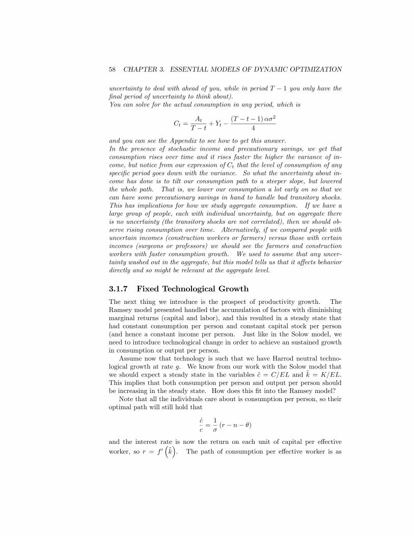
58 CHAPTER 3. ESSENTIAL MODELS OF DYNAMIC OPTIMIZATION
uncertainty to deal with ahead of you, while in period T − 1 you only have thefinal period of uncertainty to think about).You can solve for the actual consumption in any period, which is
Ct =At
T − t+ Yt −
(T − t− 1)ασ24
and you can see the Appendix to see how to get this answer.In the presence of stochastic income and precautionary savings, we get thatconsumption rises over time and it rises faster the higher the variance of in-come, but notice from our expression of Ct that the level of consumption of anyspecific period goes down with the variance. So what the uncertainty about in-come has done is to tilt our consumption path to a steeper slope, but loweredthe whole path. That is, we lower our consumption a lot early on so that wecan have some precautionary savings in hand to handle bad transitory shocks.This has implications for how we study aggregate consumption. If we have alarge group of people, each with individual uncertainty, but on aggregate thereis no uncertainty (the transitory shocks are not correlated), then we should ob-serve rising consumption over time. Alternatively, if we compared people withuncertain incomes (construction workers or farmers) versus those with certainincomes (surgeons or professors) we should see the farmers and constructionworkers with faster consumption growth. We used to assume that any uncer-tainty washed out in the aggregate, but this model tells us that it affects behaviordirectly and so might be relevant at the aggregate level.
3.1.7 Fixed Technological Growth
The next thing we introduce is the prospect of productivity growth. TheRamsey model presented handled the accumulation of factors with diminishingmarginal returns (capital and labor), and this resulted in a steady state thathad constant consumption per person and constant capital stock per person(and hence a constant income per person. Just like in the Solow model, weneed to introduce technological change in order to achieve an sustained growthin consumption or output per person.Assume now that technology is such that we have Harrod neutral techno-
logical growth at rate g. We know from our work with the Solow model thatwe should expect a steady state in the variables c = C/EL and k = K/EL.This implies that both consumption per person and output per person shouldbe increasing in the steady state. How does this fit into the Ramsey model?Note that all the individuals care about is consumption per person, so their
optimal path will still hold that
c
c=1
σ(r − n− θ)
and the interest rate is now the return on each unit of capital per effective
worker, so r = f 0³k´. The path of consumption per effective worker is as
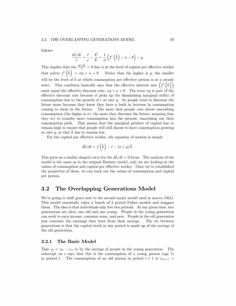
3.2. THE OVERLAPPING GENERATIONS MODEL 59
followsdc/dt
c=
c
c− E
E=1
σ
³f 0³k´− n− θ
´− g.
This implies that the dc/dtc = 0 line is at the level of capital per effective worker
that solves f 0³k´= σg + n + θ. Notice that the higher is g, the smaller
will be the level of k at which consumption per effective person is at a steadystate. This condition basically says that the effective interest rate
³f 0³k´´
must equal the effective discount rate, σg + n+ θ. The term σg is part of theeffective discount rate because it picks up the diminishing marginal utility ofconsumption due to the growth of c at rate g. So people tend to discount thefuture more because they know they have a built in increase in consumptioncoming to them in the future. The more that people care about smoothingconsumption (the higher is σ), the more they discount the future, meaning thatthey try to transfer more consumption into the present, smoothing out theirconsumption path. This means that the marginal product of capital has toremain high to ensure that people will still choose to have consumption growingat rate g, or that k has to remain low.For the capital per effective worker, the equation of motion is simply
dk/dt = f³k´− c− (n+ g) k.
This gives us a similar shaped curve for the dk/dt = 0 locus. The analysis of themodel is the same as in the original Ramsey model, only we are looking at thevalues of consumption and capital per effective worker. Once we’ve establishedthe properties of these, we can back out the values of consumption and capitalper person.
3.2 The Overlapping Generations Model
We’re going to shift gears now to the second major model used in macro, OLG.This model essentially takes a bunch of 2 period Fisher models and staggersthem. The idea is that individuals only live two periods. At any given time, twogenerations are alive, one old and one young. People in the young generationcan work to earn income, consume some, and save. People in the old generationjust consume the earnings they have from their savings. The tie betweengenerations is that the capital stock in any period is made up of the savings ofthe old generation.
3.2.1 The Basic Model
Take st = wt − c1t to be the savings of people in the young generation. Thesubscript on c says that this is the consumption of a young person (age 1)in period t. The consumption of an old person in period t + 1 is c2,t+1 =
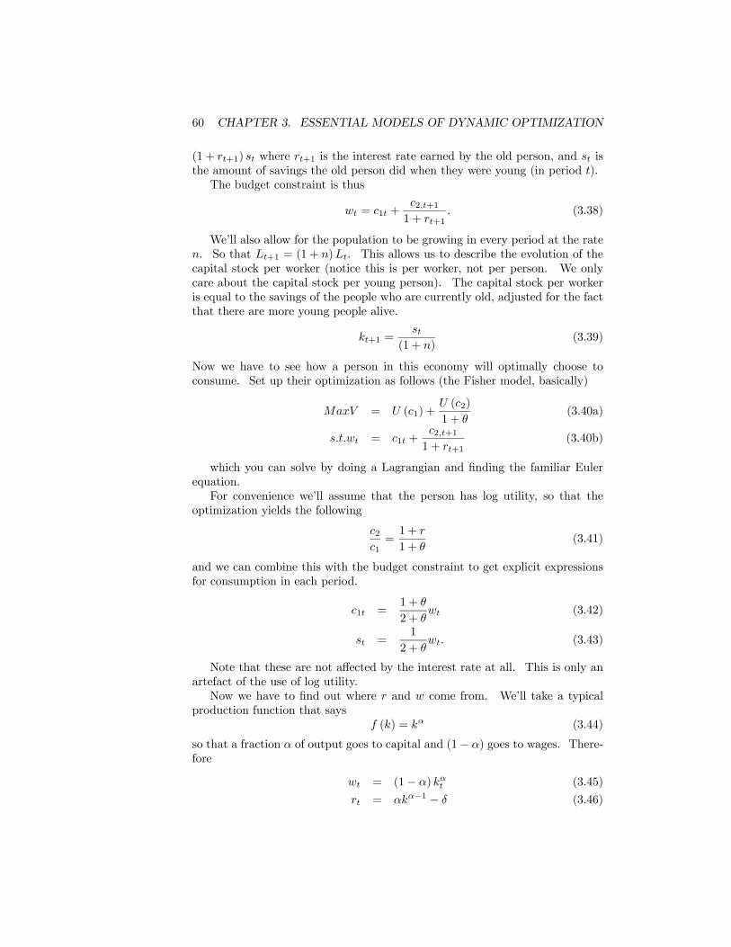
60 CHAPTER 3. ESSENTIAL MODELS OF DYNAMIC OPTIMIZATION
(1 + rt+1) st where rt+1 is the interest rate earned by the old person, and st isthe amount of savings the old person did when they were young (in period t).The budget constraint is thus
wt = c1t +c2,t+11 + rt+1
. (3.38)
We’ll also allow for the population to be growing in every period at the raten. So that Lt+1 = (1 + n)Lt. This allows us to describe the evolution of thecapital stock per worker (notice this is per worker, not per person. We onlycare about the capital stock per young person). The capital stock per workeris equal to the savings of the people who are currently old, adjusted for the factthat there are more young people alive.
kt+1 =st
(1 + n)(3.39)
Now we have to see how a person in this economy will optimally choose toconsume. Set up their optimization as follows (the Fisher model, basically)
MaxV = U (c1) +U (c2)
1 + θ(3.40a)
s.t.wt = c1t +c2,t+11 + rt+1
(3.40b)
which you can solve by doing a Lagrangian and finding the familiar Eulerequation.For convenience we’ll assume that the person has log utility, so that the
optimization yields the following
c2c1=1 + r
1 + θ(3.41)
and we can combine this with the budget constraint to get explicit expressionsfor consumption in each period.
c1t =1 + θ
2 + θwt (3.42)
st =1
2 + θwt. (3.43)
Note that these are not affected by the interest rate at all. This is only anartefact of the use of log utility.Now we have to find out where r and w come from. We’ll take a typical
production function that saysf (k) = kα (3.44)
so that a fraction α of output goes to capital and (1− α) goes to wages. There-fore
wt = (1− α) kαt (3.45)
rt = αkα−1 − δ (3.46)
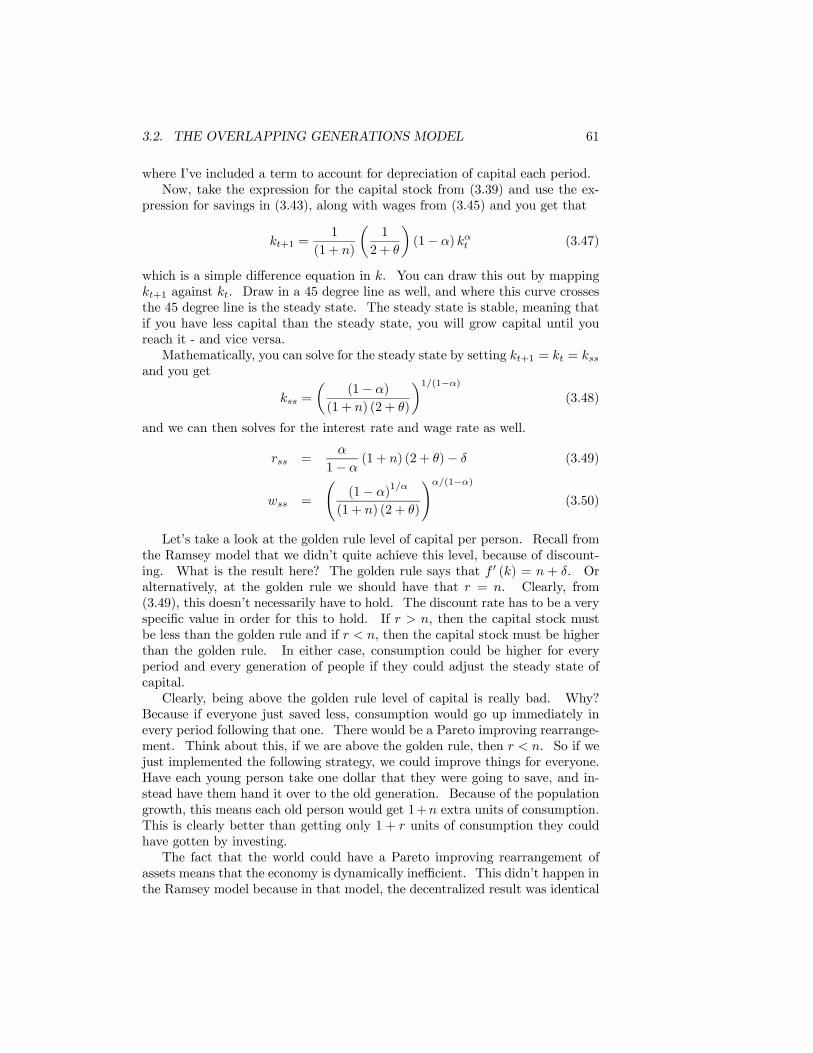
3.2. THE OVERLAPPING GENERATIONS MODEL 61
where I’ve included a term to account for depreciation of capital each period.Now, take the expression for the capital stock from (3.39) and use the ex-
pression for savings in (3.43), along with wages from (3.45) and you get that
kt+1 =1
(1 + n)
µ1
2 + θ
¶(1− α) kαt (3.47)
which is a simple difference equation in k. You can draw this out by mappingkt+1 against kt. Draw in a 45 degree line as well, and where this curve crossesthe 45 degree line is the steady state. The steady state is stable, meaning thatif you have less capital than the steady state, you will grow capital until youreach it - and vice versa.Mathematically, you can solve for the steady state by setting kt+1 = kt = kss
and you get
kss =
µ(1− α)
(1 + n) (2 + θ)
¶1/(1−α)(3.48)
and we can then solves for the interest rate and wage rate as well.
rss =α
1− α(1 + n) (2 + θ)− δ (3.49)
wss =
Ã(1− α)
1/α
(1 + n) (2 + θ)
!α/(1−α)
(3.50)
Let’s take a look at the golden rule level of capital per person. Recall fromthe Ramsey model that we didn’t quite achieve this level, because of discount-ing. What is the result here? The golden rule says that f 0 (k) = n + δ. Oralternatively, at the golden rule we should have that r = n. Clearly, from(3.49), this doesn’t necessarily have to hold. The discount rate has to be a veryspecific value in order for this to hold. If r > n, then the capital stock mustbe less than the golden rule and if r < n, then the capital stock must be higherthan the golden rule. In either case, consumption could be higher for everyperiod and every generation of people if they could adjust the steady state ofcapital.Clearly, being above the golden rule level of capital is really bad. Why?
Because if everyone just saved less, consumption would go up immediately inevery period following that one. There would be a Pareto improving rearrange-ment. Think about this, if we are above the golden rule, then r < n. So if wejust implemented the following strategy, we could improve things for everyone.Have each young person take one dollar that they were going to save, and in-stead have them hand it over to the old generation. Because of the populationgrowth, this means each old person would get 1+n extra units of consumption.This is clearly better than getting only 1 + r units of consumption they couldhave gotten by investing.The fact that the world could have a Pareto improving rearrangement of
assets means that the economy is dynamically inefficient. This didn’t happen inthe Ramsey model because in that model, the decentralized result was identical
62 CHAPTER 3. ESSENTIAL MODELS OF DYNAMIC OPTIMIZATION
to the result obtained when we assumed there was a single optimizing socialplanner in the world. In the OLG model, no one person is present across allthe periods that the economy exists (people only live for 2 of an infinite numberof periods), so no one has the ability to carry out this Pareto improving trade.
Example 18 Let’s consider an extension of the model to include social secu-rity. That is, the government is going to take some money from the youngergeneration and give it to the older generation. So each young person is taxed inthe amount d. Each old person gets the amount (1 + n) d, which holds becausethere are more young people than there are old people.What does the budget constraint look like now?
st = wt − c1t − d
c2,t+1 = (1 + rt+1) st + (1 + n) d
which gives a lifetime budget constraint of
wt +n− r
1 + rd = c1t +
c2,t+11 + r
.
If n = r, then social security has no effect on your budget constraint, as you canexactly offset its effects by borrowing or lending to get your desired consumptionpath. If n > r, then this expands the amount that a consumer can consume overtheir lifetime. If r < n, then this actually shrinks the consumption a personcan do in their life, and raises the question of why we’d have social security inthe first place. But there are other considerations (that people aren’t forwardlooking, etc..) at play in the politics of social security. One big political con-sideration is that the first generation to receive it didn’t have to pay the tax asyoungsters, so they were happy to vote in the policy that lowered utility for everysuccessive generation while raising their own utility.If we use our new budget constraint and do the Lagrangian we get optimal con-sumption in period one of
c1t =1 + θ
2 + θ
∙wt +
n− rt+11 + rt+1
d
¸and savings of
st =
µ1
2 + θ
¶ ∙wt +
(n− rt+1) (1 + θ)
1 + rt+1d
¸− d.
Combine the definitions of the capital stock, wages, and the interest rate and doa lot of algebra and you get
kt+1 =(1− α)
(1 + n) (2 + θ)kαt −
d
1 + n
∙1 + θ
2 + θ
∙n+ δ − αkα−1t
1 + αkα−1t − δ
¸+ 1
¸which looks like the old equation for the capital stock evolution in (3.47) but hasthis extra term hanging on the end. It can be shown (see the Appendix) that
3.2. THE OVERLAPPING GENERATIONS MODEL 63
this describes a relationship between kt+1 and kt that lies below the non-socialsecurity relationship. Thus social security lowers the steady state level of capitalin the economy. Now if we were oversaving before, then this could be a goodthing. If we were undersaving, then probably not.
3.2.2 Fixed Technological Growth
What happens if there is technological progress in an OLG economy? If we haveour typical Harrod neutral technological change, then our production functionis
f³k´= kα
and the associated interest rate and wages (per person) are
rt = αkα−1t − δ
wt = Et [(1− α) kαt ] .
The evoluation of capital per effective worker is
kt+1 =st
(1 + n) (1 + g)
and since savings will still just depend on wages as in (3.43), we get
st =stEt=
1
2 + θwt
=1
2 + θ
h(1− α) kαt
i.
This means that capital per effective worker evolves at
kt+1 =1
2 + θ
h(1− α) kαt
i(1 + n) (1 + g)
and essentially looks identical to before except with the extra (1 + g) termfloating around. So we get the similar result from the Solow model that as ggoes up, the actual steady state value of kss will fall. Income, on the otherhand, is increasing in g. Income per person is
yt = Etyt = Etkαss
= Et
∙(1− α)
(2 + θ) (1 + n) (1 + g)
¸α/1−αwhere I’ve plugged in the steady state value of capital per effective worker.Notice that yt goes up every period because Et goes up every period. So in theOLG model we get a very similar result to the Solow model.
64 CHAPTER 3. ESSENTIAL MODELS OF DYNAMIC OPTIMIZATION
3.2.3 Stochastic Income Shocks
Now we take the OLG model and consider how it responds to the presence ofstochastic output shocks. Output is now assumed to Cobb-Douglas with aproductivity term that is subject to random shocks, or
yt = Atkαt (3.51)
where the properties of At will be discussed later. Each individual is assumedto have log utility, and therefore is looking to maximize the following
V = ln c1 +E ln c21 + θ
(3.52)
where the E operator is the expectations term (not productivity as in priorexamples). The budget constraint is typical with
c2 = (1 + rt) (wt − c1) . (3.53)
The solution to the optimization gives us that
st =wt
2 + θ(3.54)
and by using the fact that wages are wt = (1− α)Atkαt and that kt+1 =
st/ (1 + n) we get the evolution of the capital stock as
kt+1 =(1− α)Atk
αt
(2 + θ) (1 + n). (3.55)
This is the same form as without income shocks, but notice that it doesn’t nec-essarily let us solve directly for a steady state, because the At term is stochastic.So the actual evolution of capital from period t to period t+1 changes based onthe shock received to productivity. At any given period, people act like theyare heading towards a steady state in the model, but the steady state they areheading to keeps jumping around. To see the implications of the stochasticincome further, consider a log linear version of (3.55)
ln kt+1 = lnB + α ln kt + lnAt (3.56)
where B = (1− α) / (1 + n) (2 + θ). Now take logs of (3.51) and replace it in(3.56) and you get the following
ln yt+1 = α lnB + α ln yt + lnAt+1. (3.57)
This is a first order difference equation for income, saying that income per personis autoregressive with a parameter equal to the share on capital in the economy.This is showing us that shocks to output have lingering effects on output in thefuture. How? By affecting the capital stock, the shocks affect the wage, whichaffects the savings done, and in turn affects the capital stock in the next period.
3.2. THE OVERLAPPING GENERATIONS MODEL 65
So the OLG with random shocks gives us an implication that output can followan autoregressive pattern, implying serial correlation. (Note that if we extendthe periods of the OLG beyond 2, we’ll get more periods of propogation for theshocks).This is based on the idea that lnAt+1 is a white noise error term. If it has
some kind of trend to it, as in
lnAt+1 = g + lnAt + εt (3.58)
which says that productivity has a trend g and also has a unit root, meaning thatproductivity shocks have a permanent effect on output. In this case productivityis a random walk with drift. This gives us the following for output
∆ ln yt+1 = g + α∆ ln yt + εt (3.59)
or that income growth is autoregressive and serially correlated, not the level. Ashock to output growth lingers through the following periods, until eventuallyincome growth settles back down to the rate g.

66 CHAPTER 3. ESSENTIAL MODELS OF DYNAMIC OPTIMIZATION
Chapter 4
Open EconomyMacroeconomics
We now turn to a particular application of the models and intution so far, theopen economy. To summarize how this will work, just imagine that a country iscomposed of a large number of identical individuals. With each of them solvingan identical consumption/savings problem, the amount of savings per personin the economy is simply the same as the amount of savings derived from anyindividuals problem. Let’s see how this builds up our intution about how themacroeconomics of an open economy work.
4.1 Open Economy AccountingThe first this we need to do is cover the preliminaries of national income ac-counts, so that we keep everything straight. Recall that the income identityfor a country is
Y = C + I +G+NX (4.1)
but this leaves us with a question. Is Y GDP or GNP? The answer is thatit can be either one, as long as we define imports and exports correctly. Forour purposes in this course, the distinction won’t matter that much. We’ll bethinking about capital flows, and we’ll be thinking about them in terms onlyof debt (which we’ll denote the net value of as Bt) and not about portfolioinvestment or foreign direct investment (FDI). With only debt, there is noforeign ownership of assets, and so GDP and GNP are equal.Recall that total savings is
S = I +NX (4.2)
in an open economy.The current account is the change in foreign assets in an economy, so it is
equal to NX plus interest on the assets we hold abroad, minus interest on the
67
68 CHAPTER 4. OPEN ECONOMY MACROECONOMICS
debt that we own to foreigners. So in discrete time
CAt = Bt+1 −Bt = rBt +NX (4.3)
where the r on borrowing and lending is presumed to be the same. In continuoustime this would be
CA = B = rB +NX. (4.4)
Now, we need to be specific about what exactly we mean by openness. We’llonly be considering openness to capital flows here, and won’t be thinking aboutthe nature of openness to goods trade (even though the economy can trade).So we define the following:
Definition 19 A closed economy has NX = 0 and r is endogenous.
Definition 20 A small open economy has r is exogenous and fixed at someworld rate r∗; NX is endogenous.
Definition 21 A large open economy is large enough to affect r∗, so r∗ isendogenous. Also, the level of NX is then NX = −NX∗ or the trade balancefor this large country is exactly offset by the trade balance of the rest of theworld.
4.2 Optimal Savings and the Interest Rate
For simplicity, we start again with a two period model of a country with definedlevels of GDP in each period, Y1 and Y2. We assume everyone in the economyis identical, so that the solution to any one persons two-period optimizationproblem is the same as the solution to the country’s optimization problem. Sowe can solve the optimization for this country as
maxV = U (C1) +U (C2)
1 + θ
subject to
C1 +C21 + r
= Y1 +Y21 + r
.
This is just identical to our Fisher model problem, so the answer is for thecountry to consume such that
U 0 (C1)
U 0 (C2)=1 + r
1 + θ.
How does the nature of openness affect the consumption decision? Let’stake each in turn
4.2. OPTIMAL SAVINGS AND THE INTEREST RATE 69
1. Closed economy. In this case, what happens? Well, there is no abilityfor the country as a whole to borrow or lend, so the country must beconstrained to consuming exactly C1 = Y1 and C2 = Y2. But withinthe country we have a large number of optimizing individuals, how do weensure their aggregate choices for C1 and C2 don’t violate this rule? First,recall that everyone is identical. So everyone will have the same answerto any optimization program. Second, what r could we set such thateveryone chose to exactly consume so that Y1 = C1 and Y2 = C2? Well,that would the r that solves the following equation
U 0 (Y1)
U 0 (Y2)=1 + r
1 + θ.
So even without any net borrowing or lending going on, there is still aninterest rate. This interest rate is endogenous, and clears the loanablefunds market so that people choose to consume exactly Y1 and Y2.
2. Small open economy. This is a little easier. We take r∗ as given,and solve the Euler equation for the pattern of C1 and C2. Compare C1to Y1 to find the savings of the individuals. If savings is negative, thenthe country has NX < 0 (to see this note that if S = Y − C < 0, and Iand G are positive, then it must be that NX is negative). If NX1 < 0,then with B1 = 0, it must be that CA1 < 0, or you run a current accountdeficit in the first period. In the second period, what happens? WithCA1 < 0, that means that B2 < 0, or individuals are in debt to foreigners.In period 2, then, it must be that CA2 > 0, as B3 − B2 > 0 given thatB3 = 0 by assumption. What does this imply about NX? It must bepositive.
3. Large open economy. This is easiest to think of when you have 2countries. You have to have both countries solving their Euler equations,but with a common r∗. If everyone in both countries is exactly identical,then there is zero savings in both. However, if they differ (which they canusually only through θ or the pattern of income growth) then there maybe an r∗ that makes the net savings across both countries equal to zero.That is, the borrowing of one country is offset by the lending of another.The pattern of the current account follows the small open economy patternfor the borrowing country, and is reversed for the lending country.
The upshot of all this is that the value of the autarky interest rate (thatwhich solves the Euler equation with C1 = Y1 and C2 = Y2) relative to theworld interest rate determines whether you run a current account deficit orsurplus in any given period.
70 CHAPTER 4. OPEN ECONOMY MACROECONOMICS
4.3 Growth in an Open Economy
4.3.1 Capital versus Assets
We’ll set aside the optimizing consumers for a while, and focus instead on howopenness to capital flows fits within the framework of a growing economy. Westart with the standard Solow model. With an open capital account, capitalmust flow into or out of the country until the marginal product of capital (netof depreciation) equals the world interest rate, or
r∗ = f 0 (k)− δ. (4.5)
Now we have the situation where some of the actual assets of the economy maybe owned by foreigners, so we need to distinguish between GDP and GNP. Letk represent the quantity of capital operating in the economy and let a representthe quantity of assets owned by the residents of that country. Net foreign assetsare
bt = at − kt.
Now GDP per person isGDP/L = f (k)
while GNP per person is
GNP/L = (r∗ + δ) a+ w
where the term (r + δ) is multiplied by a because we want to calculate grossnational product, not net national product.What is the wage rate? That is just what remains from GDP after payments
to capital, orw = f (k)− kf 0 (k) = f (k)− k (r∗ + δ) .
If we have Cobb-Douglas production, then f (k) = kα and we can solve for theequilibrium wage rate rate and level of capital per person by using (4.5). Thisgives us that
k =
µα
r∗ + δ
¶1/1−αand wages are then equal to
w = (1− α)
µα
r∗ + δ
¶α/1−α.
Notice that both k and w are decreasing in the world interest rate. The moreexpensive capital is to rent, the less capital is rented and the lower wages are.Now, with capital openness the capital stock will jump to exactly the abovelevel immediately, and stay constant thereafter. Wages will then be constanttoo, as we have no economic growth yet. But the stock of assets in the economywill be changing over time. Their evolution is described by
a = s ((r∗ + δ) a+ w)− (n+ δ) a
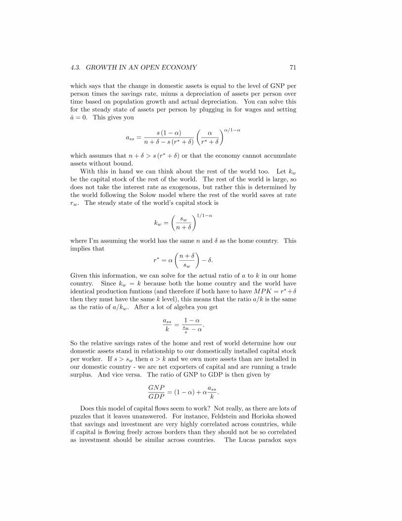
4.3. GROWTH IN AN OPEN ECONOMY 71
which says that the change in domestic assets is equal to the level of GNP perperson times the savings rate, minus a depreciation of assets per person overtime based on population growth and actual depreciation. You can solve thisfor the steady state of assets per person by plugging in for wages and settinga = 0. This gives you
ass =s (1− α)
n+ δ − s (r∗ + δ)
µα
r∗ + δ
¶α/1−αwhich assumes that n+ δ > s (r∗ + δ) or that the economy cannot accumulateassets without bound.With this in hand we can think about the rest of the world too. Let kw
be the capital stock of the rest of the world. The rest of the world is large, sodoes not take the interest rate as exogenous, but rather this is determined bythe world following the Solow model where the rest of the world saves at raterw. The steady state of the world’s capital stock is
kw =
µsw
n+ δ
¶1/1−αwhere I’m assuming the world has the same n and δ as the home country. Thisimplies that
r∗ = α
µn+ δ
sw
¶− δ.
Given this information, we can solve for the actual ratio of a to k in our homecountry. Since kw = k because both the home country and the world haveidentical production funtions (and therefore if both have to haveMPK = r∗+δthen they must have the same k level), this means that the ratio a/k is the sameas the ratio of a/kw. After a lot of algebra you get
assk=
1− αsws − α
.
So the relative savings rates of the home and rest of world determine how ourdomestic assets stand in relationship to our domestically installed capital stockper worker. If s > sw then a > k and we own more assets than are installed inour domestic country - we are net exporters of capital and are running a tradesurplus. And vice versa. The ratio of GNP to GDP is then given by
GNP
GDP= (1− α) + α
assk.
Does this model of capital flows seem to work? Not really, as there are lots ofpuzzles that it leaves unanswered. For instance, Feldstein and Horioka showedthat savings and investment are very highly correlated across countries, whileif capital is flowing freely across borders than they should not be so correlatedas investment should be similar across countries. The Lucas paradox says
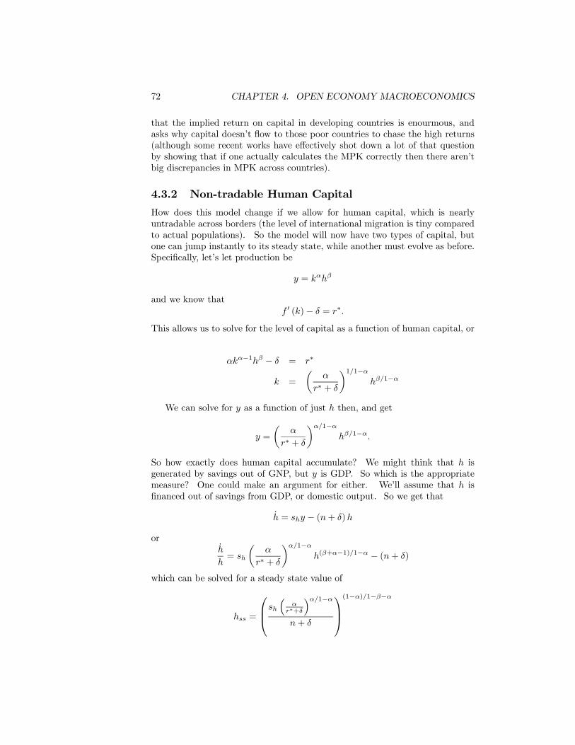
72 CHAPTER 4. OPEN ECONOMY MACROECONOMICS
that the implied return on capital in developing countries is enourmous, andasks why capital doesn’t flow to those poor countries to chase the high returns(although some recent works have effectively shot down a lot of that questionby showing that if one actually calculates the MPK correctly then there aren’tbig discrepancies in MPK across countries).
4.3.2 Non-tradable Human Capital
How does this model change if we allow for human capital, which is nearlyuntradable across borders (the level of international migration is tiny comparedto actual populations). So the model will now have two types of capital, butone can jump instantly to its steady state, while another must evolve as before.Specifically, let’s let production be
y = kαhβ
and we know thatf 0 (k)− δ = r∗.
This allows us to solve for the level of capital as a function of human capital, or
αkα−1hβ − δ = r∗
k =
µα
r∗ + δ
¶1/1−αhβ/1−α
We can solve for y as a function of just h then, and get
y =
µα
r∗ + δ
¶α/1−αhβ/1−α.
So how exactly does human capital accumulate? We might think that h isgenerated by savings out of GNP, but y is GDP. So which is the appropriatemeasure? One could make an argument for either. We’ll assume that h isfinanced out of savings from GDP, or domestic output. So we get that
h = shy − (n+ δ)h
orh
h= sh
µα
r∗ + δ
¶α/1−αh(β+α−1)/1−α − (n+ δ)
which can be solved for a steady state value of
hss =
⎛⎜⎝sh
³α
r∗+δ
´α/1−αn+ δ
⎞⎟⎠(1−α)/1−β−α
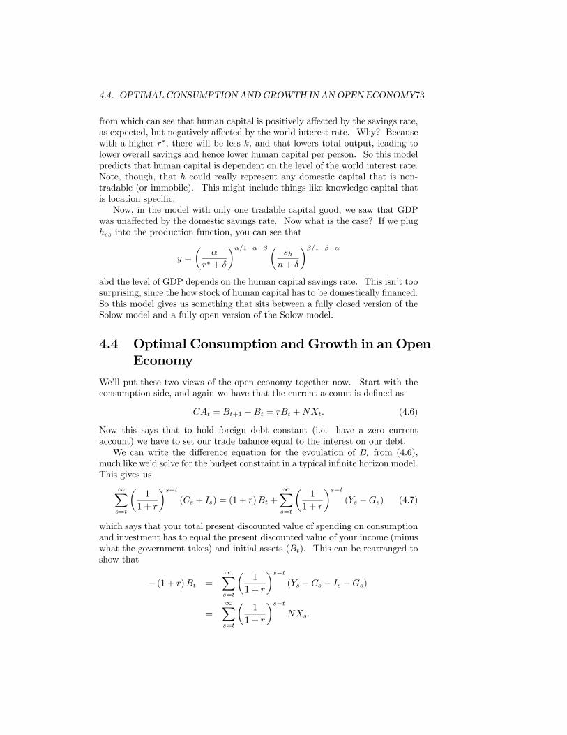
4.4. OPTIMAL CONSUMPTION ANDGROWTH IN ANOPEN ECONOMY73
from which can see that human capital is positively affected by the savings rate,as expected, but negatively affected by the world interest rate. Why? Becausewith a higher r∗, there will be less k, and that lowers total output, leading tolower overall savings and hence lower human capital per person. So this modelpredicts that human capital is dependent on the level of the world interest rate.Note, though, that h could really represent any domestic capital that is non-tradable (or immobile). This might include things like knowledge capital thatis location specific.Now, in the model with only one tradable capital good, we saw that GDP
was unaffected by the domestic savings rate. Now what is the case? If we plughss into the production function, you can see that
y =
µα
r∗ + δ
¶α/1−α−β µsh
n+ δ
¶β/1−β−αabd the level of GDP depends on the human capital savings rate. This isn’t toosurprising, since the how stock of human capital has to be domestically financed.So this model gives us something that sits between a fully closed version of theSolow model and a fully open version of the Solow model.
4.4 Optimal Consumption andGrowth in an OpenEconomy
We’ll put these two views of the open economy together now. Start with theconsumption side, and again we have that the current account is defined as
CAt = Bt+1 −Bt = rBt +NXt. (4.6)
Now this says that to hold foreign debt constant (i.e. have a zero currentaccount) we have to set our trade balance equal to the interest on our debt.We can write the difference equation for the evoulation of Bt from (4.6),
much like we’d solve for the budget constraint in a typical infinite horizon model.This gives us
∞Xs=t
µ1
1 + r
¶s−t(Cs + Is) = (1 + r)Bt +
∞Xs=t
µ1
1 + r
¶s−t(Ys −Gs) (4.7)
which says that your total present discounted value of spending on consumptionand investment has to equal the present discounted value of your income (minuswhat the government takes) and initial assets (Bt). This can be rearranged toshow that
− (1 + r)Bt =∞Xs=t
µ1
1 + r
¶s−t(Ys − Cs − Is −Gs)
=∞Xs=t
µ1
1 + r
¶s−tNXs.
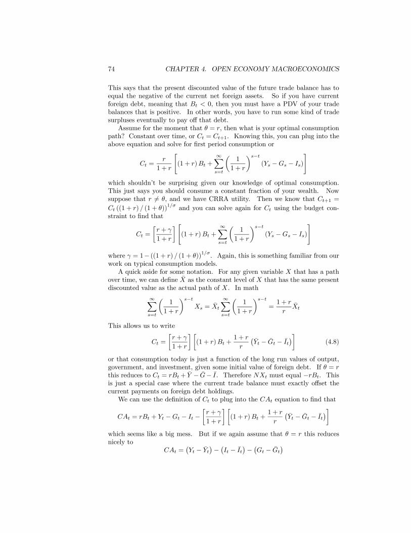
74 CHAPTER 4. OPEN ECONOMY MACROECONOMICS
This says that the present discounted value of the future trade balance has toequal the negative of the current net foreign assets. So if you have currentforeign debt, meaning that Bt < 0, then you must have a PDV of your tradebalances that is positive. In other words, you have to run some kind of tradesurpluses eventually to pay off that debt.Assume for the moment that θ = r, then what is your optimal consumption
path? Constant over time, or Ct = Ct+1. Knowing this, you can plug into theabove equation and solve for first period consumption or
Ct =r
1 + r
"(1 + r)Bt +
∞Xs=t
µ1
1 + r
¶s−t(Ys −Gs − Is)
#which shouldn’t be surprising given our knowledge of optimal consumption.This just says you should consume a constant fraction of your wealth. Nowsuppose that r 6= θ, and we have CRRA utility. Then we know that Ct+1 =
Ct ((1 + r) / (1 + θ))1/σ and you can solve again for Ct using the budget con-straint to find that
Ct =
∙r + γ
1 + r
¸"(1 + r)Bt +
∞Xs=t
µ1
1 + r
¶s−t(Ys −Gs − Is)
#
where γ = 1− ((1 + r) / (1 + θ))1/σ. Again, this is something familiar from our
work on typical consumption models.A quick aside for some notation. For any given variable X that has a path
over time, we can define X as the constant level of X that has the same presentdiscounted value as the actual path of X. In math
∞Xs=t
µ1
1 + r
¶s−tXs = Xt
∞Xs=t
µ1
1 + r
¶s−t=1 + r
rXt
This allows us to write
Ct =
∙r + γ
1 + r
¸ ∙(1 + r)Bt +
1 + r
r
¡Yt − Gt − It
¢¸(4.8)
or that consumption today is just a function of the long run values of output,government, and investment, given some initial value of foreign debt. If θ = rthis reduces to Ct = rBt+ Y − G− I. Therefore NXt must equal −rBt. Thisis just a special case where the current trade balance must exactly offset thecurrent payments on foreign debt holdings.We can use the definition of Ct to plug into the CAt equation to find that
CAt = rBt + Yt −Gt − It −∙r + γ
1 + r
¸ ∙(1 + r)Bt +
1 + r
r
¡Yt − Gt − It
¢¸which seems like a big mess. But if we again assume that θ = r this reducesnicely to
CAt =¡Yt − Yt
¢−¡It − It
¢−¡Gt − Gt
¢
4.4. OPTIMAL CONSUMPTION ANDGROWTH IN ANOPEN ECONOMY75
and this tells us that the current account is just equal to the deviations ofoutput, government and investment from their long run values. The currentaccount is therefore only a way to temporarily smooth consumption when wehave periods of shocks to our long run path. This comes our modelling theeconomy as similar to an individual who uses the financial markets to smooththeir consumption. If r 6= θ, then this is modified slightly, but the intuitionremains that the current account is a smoothing mechanism.Now we can consider adding economic growth into this mix. Define output
more specifically as
Yt = AtKαt
At+1 = (1 + g)1−αAt
so that in the steady state, output and capital per worker will grow at rate g.The adjustment 1− α on the growth of A just makes sure this works out.This is an open economy, so the interest rate will always be equal to the
world interest rate, r∗. We will always assume that r∗ > g, otherwise peoplewould be able to grow completely out of debt. This pins down the marginalproduct of capital (assume no depreciation) and that pins down the capitalstock.
r∗ = αAtKα−1t (4.9)
Kt =
µαAt
r∗
¶1/1−α(4.10)
Since capital will grow at rate g (given the above equation), then investmentmust be equal to the following
It = Kt+1 −Kt = g
µαAt
r∗
¶1/1−α.
Substitute the equation for capital in (4.10) into production and you get
Yt = A1/1−αt
³ αr∗
´α/1−αand using this we can write investment as a proportion of output as
It =³αgr∗
´Yt.
We’ll just assume now that government spending is a constant fraction oftotal output, β (and that β < 1 − αg
r∗ . So output minus investment andgovernment spending is
Ys − Is −Gs = (1 + g)s−t³1− αg
r∗− β
´Yt
76 CHAPTER 4. OPEN ECONOMY MACROECONOMICS
which says that output minus investment and government at time s is a functionof output at time t. Consumption at time t can be solved for now, using ourexpression from (4.8). This gives
Ct =
∙r∗ + γ
1 + r∗
¸"(1 + r∗)Bt +
³1− αg
r∗− β
´Yt
∞Xs=t
µ(1 + g)
(1 + r∗)
¶s−t#
and this can be evaluated to see that
Ct =
∙r∗ + γ
1 + r∗
¸ ∙(1 + r∗)Bt +
1 + r∗
r∗ − g
³1− αg
r∗− β
´Yt
¸= (r∗ + γ)Bt +
r∗ + γ
r∗ − g
³1− αg
r∗− β
´Yt
This and the definitions of investment and outpu will allow us to specify thecurrent account now, which gives us
CAt = −γBt −g + γ
r∗ − g
³1− αg
r∗− β
´Yt.
So the current account again depends on the state of foreign debt (Bt) and onthe current level of income. To see more clearly how the economy responds todifferences in g or r∗, it will be useful to consider the ratio of foreign debt toincome, rather than the current account specifically. So
Bs+1 = Bs + CAs
Ys+1 = (1 + g)Ys
and their ratio is then
Bs+1
Ys+1=1− γ
1 + g
Bs
Ys− g + γ
r∗ − g
³1− αg
r∗− β
´ 1
1 + g.
This perhaps doesn’t look like it is helping. But notice that we have a differenceequation in B/Y that is linear. What is the steady state?
Bs
Ys= −
1− αgr∗ − β
r∗ − g
which you’ll notice is always negative (recall that r∗ > g by assumption always).So if you’re at this steady state, you’ve got a permanent level of foreign debt.However, will you end up at this steady state? Consider first the case wheng > −γ, and this means that the slope of the difference equation is < 1 andthe intercept is negative. In this case the steady state is stable, meaning thatwhatever level of B/Y I start with, I’ll end up at this steady state with foreigndebt. What is happening? The growth rate of output is greater than the growthrate of consumption (recall that γ measures the inverse of the growth rate ofconsumption). The growth rate of consumption is low because the country
4.4. OPTIMAL CONSUMPTION ANDGROWTH IN ANOPEN ECONOMY77
has high initial consumption, which is funded by borrowing from foreigners.Eventually, the country spends all of its income on paying back this debt. Infact the present value of consumption is exactly equal to the present value ofthe foreign debt.Now, consider when g < −γ or consumption growth is higher than economic
growth. In this case the steady state is unstable (the intercept is greater thanzero and the slope is greater than one). If the country starts with a smalllevel of foreign debt, then it can pay this back quite easily given that it has lowinitial consumption and high consumption growth. The country pays off it’sdebt and starts to actually acquire positive foreign assets - lending money toother countries.Thus the nature of foreign debt relative to output depends primarily on the
preference parameters for consumption, and also on the exogenous growth rate.

78 CHAPTER 4. OPEN ECONOMY MACROECONOMICS

Chapter 5
Endogenous Growth Models
In this chapter we return to the topic of economic growth, but we want to thinkagain about where this growth comes from. In the Solow model, sustainedeconomic growth (meaning increases in income per person) are only possiblethrough purely exogenous growth - g. This has two primary problems, the firsttheoretical and the other empirical.
• Theoretical: We haven’t actually explained anything if we just assertthat growth is exogenous. Why is g = 0.02 in the U.S. and not higher orlower in the long run? Why is g low in Nigeria and high in South Korea?The Solow model, and models with exogenous technological progress ingeneral, have the unappealling feature that some of the most importantfeatures of economies are actually not explained. So we want to solve thatby trying to write down models that actually generate the growth rate ofoutput per person internally, and ideally as the result of some optimizingdecision by individuals.
• Empirical: The Solow model does have growth in it, only out of the steadystate. If different countries were simply different distances away from theirsteady states, then differences in growth rates would be explained by thisdistance, and not by g. When we examine the data, though, this doesn’tappear to be the case. Additionally, if we do some simple accounting forthe sources of growth within countries or across countries, we see that thetotal factor productivity is the most important explanation for growth anddevelopment. So the Solow model, which is a model of capital accumula-tion, doesn’t actually address the most important component of economicgrowth.
So we’re going to examine this empirical evidence in a little more detailfirst, covering the convergence of countries to their steady states as well as de-velopment and growth accounting. This will show us that we need somethingmore than just the Solow model. This will lead us to think about endoge-nous growth models, starting with mechanical ones without optimizing agents,
79
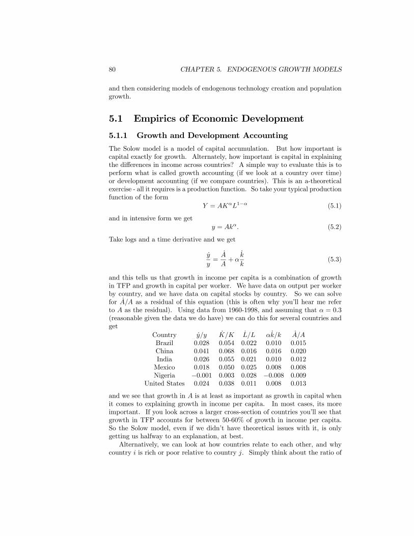
80 CHAPTER 5. ENDOGENOUS GROWTH MODELS
and then considering models of endogenous technology creation and populationgrowth.
5.1 Empirics of Economic Development
5.1.1 Growth and Development Accounting
The Solow model is a model of capital accumulation. But how important iscapital exactly for growth. Alternately, how important is capital in explainingthe differences in income across countries? A simple way to evaluate this is toperform what is called growth accounting (if we look at a country over time)or development accounting (if we compare countries). This is an a-theoreticalexercise - all it requires is a production function. So take your typical productionfunction of the form
Y = AKαL1−α (5.1)
and in intensive form we gety = Akα. (5.2)
Take logs and a time derivative and we get
y
y=
A
A+ α
k
k(5.3)
and this tells us that growth in income per capita is a combination of growthin TFP and growth in capital per worker. We have data on output per workerby country, and we have data on capital stocks by country. So we can solvefor A/A as a residual of this equation (this is often why you’ll hear me referto A as the residual). Using data from 1960-1998, and assuming that α = 0.3(reasonable given the data we do have) we can do this for several countries andget
Country y/y K/K L/L αk/k A/ABrazil 0.028 0.054 0.022 0.010 0.015China 0.041 0.068 0.016 0.016 0.020India 0.026 0.055 0.021 0.010 0.012Mexico 0.018 0.050 0.025 0.008 0.008Nigeria −0.001 0.003 0.028 −0.008 0.009
United States 0.024 0.038 0.011 0.008 0.013
and we see that growth in A is at least as important as growth in capital whenit comes to explaining growth in income per capita. In most cases, its moreimportant. If you look across a larger cross-section of countries you’ll see thatgrowth in TFP accounts for between 50-60% of growth in income per capita.So the Solow model, even if we didn’t have theoretical issues with it, is onlygetting us halfway to an explanation, at best.Alternatively, we can look at how countries relate to each other, and why
country i is rich or poor relative to country j. Simply think about the ratio of
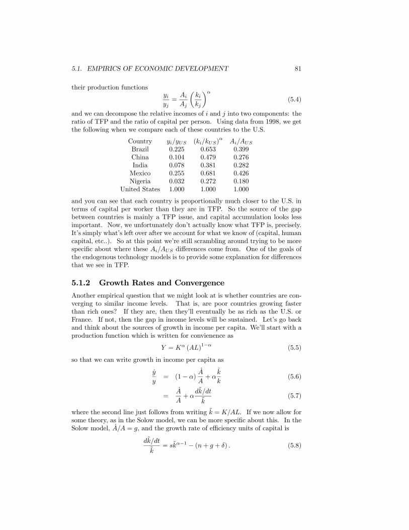
5.1. EMPIRICS OF ECONOMIC DEVELOPMENT 81
their production functionsyiyj=
Ai
Aj
µkikj
¶α(5.4)
and we can decompose the relative incomes of i and j into two components: theratio of TFP and the ratio of capital per person. Using data from 1998, we getthe following when we compare each of these countries to the U.S.
Country yi/yUS (ki/kUS)α
Ai/AUS
Brazil 0.225 0.653 0.399China 0.104 0.479 0.276India 0.078 0.381 0.282Mexico 0.255 0.681 0.426Nigeria 0.032 0.272 0.180
United States 1.000 1.000 1.000
and you can see that each country is proportionally much closer to the U.S. interms of capital per worker than they are in TFP. So the source of the gapbetween countries is mainly a TFP issue, and capital accumulation looks lessimportant. Now, we unfortunately don’t actually know what TFP is, precisely.It’s simply what’s left over after we account for what we know of (capital, humancapital, etc..). So at this point we’re still scrambling around trying to be morespecific about where these Ai/AUS differences come from. One of the goals ofthe endogenous technology models is to provide some explanation for differencesthat we see in TFP.
5.1.2 Growth Rates and Convergence
Another empirical question that we might look at is whether countries are con-verging to similar income levels. That is, are poor countries growing fasterthan rich ones? If they are, then they’ll eventually be as rich as the U.S. orFrance. If not, then the gap in income levels will be sustained. Let’s go backand think about the sources of growth in income per capita. We’ll start with aproduction function which is written for convienence as
Y = Kα (AL)1−α (5.5)
so that we can write growth in income per capita as
y
y= (1− α)
A
A+ α
k
k(5.6)
=A
A+ α
dk/dt
k(5.7)
where the second line just follows from writing k = K/AL. If we now allow forsome theory, as in the Solow model, we can be more specific about this. In theSolow model, A/A = g, and the growth rate of efficiency units of capital is
dk/dt
k= skα−1 − (n+ g + δ) . (5.8)
82 CHAPTER 5. ENDOGENOUS GROWTH MODELS
So growth in income per capita can be written as
y
y= g + α
hskα−1 − (n+ g + δ)
i(5.9)
and notice that the term in brackets is a non-linear function. We can evaluatethis term in brackets by doing a first-order Taylor expansion and linearizingaround the steady state value. So start by defining the bracketed term as
h³ln k
´= αse(α−1) ln k − α (n+ g + δ) (5.10)
and the linear expansion around k∗ is defined as
h³ln k∗
´+ h0
³ln k∗
´³ln k − ln k∗
´. (5.11)
Now, we know that in the steady state h³ln k∗
´= 0 (plug in the steady
state value into h³ln k
´and you’ll see it comes out to zero). Next, note that
h0³ln k∗
´= (α− 1)αse(α−1) ln k∗ (5.12)
and given the definition of the steady state value of k∗ = (s/ (n+ g + δ))1−α
we can plug in to this equation and get
h0³ln k∗
´= (α− 1)α (n+ g + δ) . (5.13)
Finally, note that ln y = α ln k and ln y∗ = α ln k∗. We can put all this infor-mation into (5.11) and (5.9) we get that
y
y= g + (1− α) (n+ g + δ) (ln y∗ − ln y) . (5.14)
This equation tells us that growth in income per capita has two components.The first is regular technological growth (g) and the second is growth due toconvergence to the steady state. The farther a country is from steady state(ln y∗ − ln y is larger), the faster a country grows. Why? Because of decreasingreturns to capital. The less capital you have, the higher the marginal productof that capital, and the faster you grow when you add a unit of capital. Ifyou are at your steady state, you’ll just grow at the rate g. Note that theactual speed of convergence depends on your fertility rate, on g itself, and onthe depreciation rate (but NOT on the savings rate).What this tells us is that - holding everything else equal - poor countries
should grow faster than rich countries. Does this hold up in the data? No, notdirectly. The growth rates of the developed world are generally as high or higherthan the growth rates of developing countries. Aside from several countries thatare making the "leap" (India, China, Asian Tigers). However, not everything
5.1. EMPIRICS OF ECONOMIC DEVELOPMENT 83
is equal. Countries may have different steady states or g, and in that case wemight get any kind of pattern to growth rates that we can think of. Whatseems to be true, given the data, is that once we control for factors affectingthe steady state (savings, fertility, etc..), the YES, it is true that countries withlower income per capita do grow faster than countries with high income percapita. So we have what we call "conditional convergence". The structure ofthe Solow model does seem to hold up. But it leaves us wondering why thesteady state’s themselves differ in the first place, which the Solow model can’texplain.
5.1.3 Interest Rate Differentials
The last empirical issue to consider is the nature of interest rates. These reflectthe marginal product of capital in a country, and so any growth model that tellsus the size of the capital stock should be able to tell us what interest rates are.If we have countries with identical production functions of
y = Akα (5.15)
then the interest rate isr = αAkα−1 − δ. (5.16)
If we take the U.S. as a baseline, we might think that real returns (r) are equalto 5%. With depreciation of around 5%, this would imply that the marginalproduct of capital must be about 10%.If we look at a developing country with income per capita of only about 20%
of the U.S., we have thatyiyus
=AkαiAkαUS
=1
5(5.17)
and for now let’s assume that technology in the countries is the same. So thatmeans that
kikus
=1
125(5.18)
if we assume that α = 1/3. If this is true, then the marginal product of capitalin country i must be
MPKi
MPKus=
µkikus
¶α−1=
µ1
125
¶−2/3= 25 (5.19)
and therefore the interest rate in country i must be
ri = 25 (10%)− 5% = 245% (5.20)
which seems aboslutely too incredible to be true. We should see capital flowfrom the U.S. to this country to reap the rewards of a 245% return on capital.And we don’t see anything like these kinds of differences.However, we could assume that interest rates ARE equalized between coun-
tries, and then back out what the implied differences in A are across countries
84 CHAPTER 5. ENDOGENOUS GROWTH MODELS
that can account for this. In other words, we think the marginal product ofcapital should be equated across countries, and if so we get
Aikα−1i = Ausk
α−1us (5.21)
Ai
Aus=
µkuski
¶1−α(5.22)
and in the worst cases we observe something like kuski= 50. This implies that
AiAus
= 13.6. Is this realistic? Do we really think that one country is reallyfourteen times more production than another? This seems way too big to makesense.So it would be nice if our models of growth were consistent with equalized
rates of return across countries (because we think international financial marketswork to some extent) but don’t require crazy differences in TFP to generatethem.
5.2 Basic ModelsThe endogenous growth literature is motivated by an attempt to explain whereSolow’s g comes from. We see sustained, stable growth in most developedeconomies, and these models are an attempt to show how this can arise througheconomic behavior, as opposed to the remarkable coincidence that technologygrows at some constant rate per year. These models, though, are less usefulin describing differences across countries, as they don’t seem to capture theimportant factors separating developing countries from the rich world.
5.2.1 The AK Model
Think about the Solow model with Y = Akα and a growth rate of capital of
k
k= sAkα−1 − (n+ δ) .
We know that the growth rate of capital (and therefore of output) increases aswe get away from the steady state. Imagine that as we are approaching thesteady state, we have a shift up in the savings rate. What happens? There isa temporary increase in growth again (as we’re now far away from the steadystate) but this growth will eventually die down again as well.Now imagine this scenario again, but with α very close to one If this pa-
rameter is close to one, then the sAkα−1 is getting less sloped, and starting tolook like a straight line. In this case, the increase in growth when s goes up isvery large, and it takes a very long time for the growth effect to die out. In thelimit, as α = 1 what happens to the growth rate of capital?
k
k= sA− (n+ δ)
5.2. BASIC MODELS 85
What does this tell us? Notice that there is nothing in this equation thatimplies that k
k ever has to fall. Assuming sA > (n+ δ), then the growth rate ofcapital is constant and positive. The growth rate of output in this case is theny/y = k/k, or output per person is growing constantly as well. The only thingthat affects this growth rate is the preference parameters s, n, and δ. So wehave sustained growth without relying on exogenous technology creation. Thisseems to be an improvement.What does the AK model imply?
1. We have the marginal product of capital as f 0 (k) = A, so r = A−δ. Sincewe presume that A is common across countries (sometimes) this impliesthat there should be no differences in interest rates across countries. Thisis a big improvement over the Solow model, and seems to match the datapretty well.
2. What does the AK model imply about the relationship of income level andincome growth? The AK model says there is no relationship - a countryhas a constant growth rate regardless of its initial income level. Thisseems to be good, because in the data we don’t see a clear relationshipbetwee income levels and growth.
3. Savings are positively related to growth, where in the Solow model savingsare related to income levels.
4. Population growth is negatively related to growth, where in the Solowmodel population growth lowers the income level.
So does the AK model have any justification? All we’ve done is assert thatα = 1, and recall that α is roughly synonymous with capital’s share in totaloutput, and empirically this is closer to 1/3. So how does the AK model getα = 1?The basic story is that there are externalities to production. Assume the
actual production function is Y = AKαLβ . But now, the level of technology Ais a function of how much capital exists in the economy. Maybe more capitalmeans more specialization and this has productivity gains due to comparativeadvantage. This could also be through learning by doing, in that we learnbetter techniques every time we install new capital.So let’s call the level of A
A =
µK
L
¶γ.
This makes the production function
Y = KαLβkγ .
Now, we assume that α + β = 1, or there are constant returns to scale foreach firm. This is because each firm takes kγ as a given. Firms don’t take
86 CHAPTER 5. ENDOGENOUS GROWTH MODELS
into account that an increase in their own capital stock will actually increaseeveryone’s A level. Also, because the kγ term is just an externality, the firmsdon’t have to make factor payments on this. This means that the productionfunction looks like this for a given firm i
Yi = Kαi L
1−αi kγ
which implies that each firm pays out 1 − α of its output to labor. Settingα = 1/3 we can match the aggregate data pretty well.Looking again at aggregate output, if we consider the per person output, we
gety = kαkγ
which gives us the AK model if α+γ = 1. So the AK model can be justified if weassume that firms have some externality that they receive to their productivitybased on the aggregate capital labor ratio. Notice that this also means thatthe economy does not optimally invest in capital. The marginal product ofcapital from the perspective of individual firms is only αkα+γ−1 while from theaggregate perspective it is (α+ γ) kα+γ−1.The biggest issue with the AK model is probably that it implies that the
externalities are enourmous. The elasticity of output with respect to capital,based solely on the externality is
∂y
∂k
k
y= γ
or a 1% increase in the capital stock leads to a 0.67% increase in output, justdue to the externality. This seems awfully high.
5.2.2 Generalizing Endogenous Growth
So the AK model delivers endogenous growth by building in something to theSolow model that eliminates the decreasing returns to capital. In general, mod-els that have decreasing returns to the accumulable factors (such as our basicSolow human capital model) all have zero steady state growth by themselves(that is, they require exogenous technological growth). Models that somehowgenerate constant returns (or increasing returns) to accumulable factors willdeliver endogenous growth. Let’s see how this works a little more generally.Take a general production function of the form
Y = AXαLβ
where X represents accumulable factors of production (physical capital, humancapital, etc). L is population, as normal. Also assume we have a constantsavings rates (recall that this really doesn’t matter, the endogenous savings ratesin the Ramsey model give us the same steady state analysis). Then the changein the stock of factors can be written as
5.2. BASIC MODELS 87
X = sAXαLβ − δX
where there is some depreciation factor. If population grows at the rate n, andwe rewrite everything in per capita terms using small letters, then we get
x = sAxαLα+β−1 − (δ + n)x (5.23)x
x= sAxα−1Lα+β−1 − (δ + n)
which should look vaguely familiar at this point.So now, if this model has a steady state, it must be that x is growing at
a constant rate. We don’t know what it is, but let’s label this rate γ. Andtherefore in steady state
x
x= γ.
The value of A isn’t going to impact the conclusions at this point, so we cansafely assume it to be equal to one (if you don’t trust me, follow through onthe math with A included and you’ll see it always cancels). So we can use ourequation of motion for x in (5.23) to see that
γ = sAXα−1Lα+β−1 − (δ + n) .
What we’re interested in is NOT the size of X and L that make this hold.What we want to know is what restrictions on the parameters of the modelyield constant growth. In other words, the LHS of the above equation is notchanging - the growth rate is constant. So what makes the RHS of the aboveequation stay constant as well? To see, let’s take the time derivative of thisequation on both sides.
0 = s³(α− 1)xα−2xLα+β−1 + xα−1 (α+ β − 1)Lα+β−2L
´0 = sxα−1Lα+β−1
Ã(α− 1) x
x+ (α+ β − 1) L
L
!
0 = (α− 1) xx+ (α+ β − 1) L
L0 = (α− 1) γ + (α+ β − 1)n
and using this last expression we can characterize all the possible circum-stances under which steady state growth at rate γ is possible.
1. α+ β = 1 (Constant Returns to Scale)
(a) α < 1, β < 1 =⇒ γ = 0 (Solow Model)
88 CHAPTER 5. ENDOGENOUS GROWTH MODELS
(b) β = 0, α = 1 =⇒ γ > 0 (AK Model)
2. α+ β > 1 (Increasing Returns to Scale)
(a) α < 1, β < 1
i. n > 0 =⇒ γ = α+β−11−α n
ii. n = 0 =⇒ γ = 0
(b) β > 0, α = 1
i. n > 0 =⇒ no feasible solutionii. n = 0 =⇒ any value of γ is feasible
So whatever the details of your endogenous growth model, in order to gen-erate perpetual growth without exogenous technological progress you must beable to reduce the model to a form similar to either 1.b, 2.a.i, or 2.b.ii.The point is that any model that hopes to permit perpetual long-run growth
has to boil down to a structure in which there are constant returns to scale for theset of factors that can be jointly accumulated. Another way of looking at thisis to consider what your production function looks like in intensive form. Thatis, does per person output have constant or decreasing returns to scale? If youhave decreasing returns in the intensive form, you cannot achieve endogenousgrowth. If you have constant returns, you can achieve endogenous growth.
Example 22 Let’s think about a production function that includes human cap-ital and has different properties.
Y = Kαh1−α (EL)1−α
= KαH1−α
where H = hEL or H is the total amount of human effort that is brought tobear in production and h measures the per efficiency unit value of this. So wehave a production function that satisfies the AK model conditions (1.b above) -it has constant returns to the accumulable factors (K and H), and a coefficientof zero on labor. The intensive production function can be written as
y = kαh1−α.
Notice that this intensive form has constant returns to scale, so that if we doubledk and h we’d double output. This changes our expectations for the steady state.Now, even as k and h increase, output is increasing just as fast, so that we’llbe able to continue to grow both k and h indefinitely. The equations of motionare the similar to before, so that we get
k
k= sk
kαh1−α
k− (n+ δ + g)
h
h= sh
kαh1−α
h− (n+ δ + g)
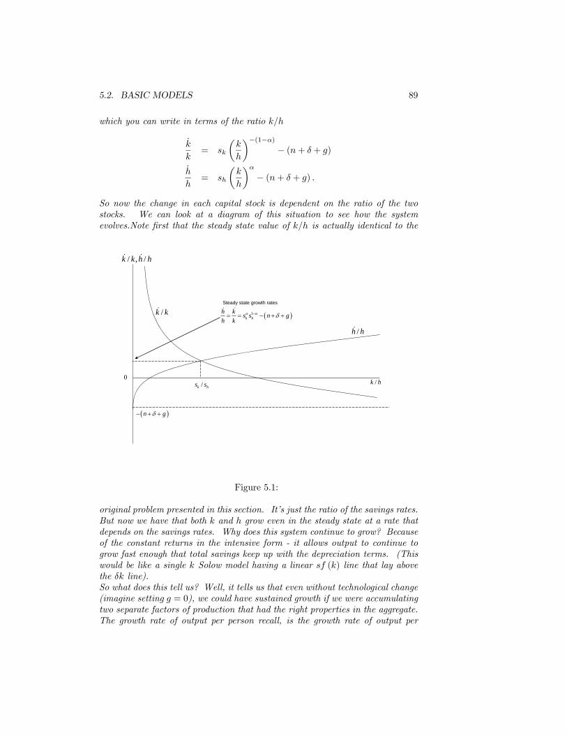
5.2. BASIC MODELS 89
which you can write in terms of the ratio k/h
k
k= sk
µk
h
¶−(1−α)− (n+ δ + g)
h
h= sh
µk
h
¶α− (n+ δ + g) .
So now the change in each capital stock is dependent on the ratio of the twostocks. We can look at a diagram of this situation to see how the systemevolves.Note first that the steady state value of k/h is actually identical to the
/k h
/ , /k k h h& &
/k k&
/h h&
/k hs s0
( )n gδ− + +
( )1k h
h k s s n gh k
α α δ−= = − + +& &Steady state growth rates
Figure 5.1:
original problem presented in this section. It’s just the ratio of the savings rates.But now we have that both k and h grow even in the steady state at a rate thatdepends on the savings rates. Why does this system continue to grow? Becauseof the constant returns in the intensive form - it allows output to continue togrow fast enough that total savings keep up with the depreciation terms. (Thiswould be like a single k Solow model having a linear sf (k) line that lay abovethe δk line).So what does this tell us? Well, it tells us that even without technological change(imagine setting g = 0), we could have sustained growth if we were accumulatingtwo separate factors of production that had the right properties in the aggregate.The growth rate of output per person recall, is the growth rate of output per
90 CHAPTER 5. ENDOGENOUS GROWTH MODELS
effective unit plus the growth rate of E. The growth rate of output per effectiveunit is
y/y = αk/k + (1− α) h/h
= sαks1−αh − (n+ δ + g)
so the growth rate of output per person is.
(Y/L)
Y/L= sαks
1−αh − (n+ δ) .
And our standard of living now doesn’t depend at all on the rate of g, only onthe savings rates relative to the depreciation rates. This is a simple exampleof an endogenous growth model in which the actual growth of output per persondepends only on preference parameters and not on an exogenous rate g.You can also use the diagram to analyze what happens to k/h when there is achange in the savings rates. One of the curves (or both) may shift, creatingsome transitional growth to a new steady state value of k/h, and there will beplenty of chances on homeworks to see how this operates.
5.2.3 Lucas’ Human Capital Model
Lucas provided a slightly different outlook on the accumulation of human cap-ital, incorporating the fact that it involves a time commitment, as opposed tosimply financial backing. The production function is
Y = Kα (uhL)1−α (5.24)
where L is labor, h is human capital per person, and u is the fraction of timespent working (so it lies between zero and one). In per capita terms thisbecomes
y = kα (uh)1−α (5.25)
and so production, in the intensive form, is constant returns to scale, and wewill have endogenous growth. Note that nothing about the mechanics of u wedescribe can change this, it’s a property of the production function alone.Capital accumulates as expected
k = y − c− (n+ δ) k (5.26)
and human capital accumulates as follows
h = φh (1− u) (5.27)
which says that human capital is accumulated in a constant returns to scalemanner. If we double the time spent on education, we double the growth rateof human capital.One can solve this problem in a Ramsey setting with optimizing agents, but
we know that in the steady state this isn’t any different from the Solow model.
5.3. ENDOGENOUS TECHNOLOGY CREATION 91
So we’re going to do the Solow version of this, which just assumes a constantsavings rate of s, and therefore c = (1− s) y and the capital accumulationequation is just what you’d expect.Look at the growth rate of capital
k
k= s
µk
h
¶1−αu1−α − (n+ δ) (5.28)
and map this against the growth rate of human capital
h
h= φ (1− u) (5.29)
on a graph with k/h on the x-axis. The human capital growth rate is constant,and k/k will, in steady state, just be equal to the growth rate of human capital.One of the things to take out of this model is that the factor that dependson itself (human capital) will drive the growth rate. Physical capital growthdepends on both (because it depends on total output) and therefore it will haveto fall in line with human capital.Growth in output per person is
y
y= α
k
k+ (1− α)
h
h(5.30)
and therefore the growth rate of output per person equals h/h as well.There are transitional dynamics, which can be parsed out of the diagram
when the initial k/h ratio isn’t exactly equal to the steady state value. Oneinteresting experiment is to ask what would happen if you lower the value ofu (thus raising the growth rate of human capital). Note that the level of yhas to fall initially, but then will grow faster, and eventually income will behigher overall. However, the choice of u can then be seen to depend on yourdiscounting of the future path of income.
5.3 Endogenous Technology Creation
The models so far have developed endogenous growth through very specificchoices about the parameters of the production function. Note that even if theproduction does allow for growth, this doesn’t mesh with our observations aboutincreasing technological sophistication over time. In addition, it doesn’t meshwith our empirical observations about how important TFP is. So another lineof research on endogenous growth looks to explain the increase in technologyeconomically. That is, what are the incentives to invent better ways of doingthings?These models will depart from the standard constant returns to scale, perfect
competition set up we’ve used so far. Why? With CRS and perfect competition,all output is used up in paying for the factors of production. There is nothing
92 CHAPTER 5. ENDOGENOUS GROWTH MODELS
left over, and so there is no output left to reward inventive activity. What themodels in this section will do is introduce some kind of market imperfectionsthat allow for profits to accrue to those who know better technology. Thiscreates incentives to generate new technology, and we’ll get growth.
5.3.1 Increasing Variety of Intermediate Goods
The first major family of models thinks of technology as the introduction of newgoods. This is easy to conceive of mentally, and it must matter to some extent.This model will introduce the idea of monopolistic competition, which will lookcomplicated, but is a very common way to generate profits for firms within amodel.There is no capital (but we could add it if we wanted to). There is a
constant supply of labor, L. Y is output, which is produced using labor andintermediate goods (denoted X). N is the number of these intermediate goodsin the economy. Intermediate goods are not capital, they are flows of inputsinto final production.Let’s think about firms in the final goods sector (those that use labor and
intermediate goods). Output for any final goods firm is as follows
Yi = L1−αi
NXj=1
Xαij (5.31)
where i indexes the firm, and j indexes the intermediate goods. Note the follow-ing: 1) the use of a single intermediate good does NOT affect the productivityof the others, 2) there is decreasing marginal productivity of each intermediategood, and 3) this means that all intermediate goods will be used in the samequantity. The way to see this is to imagine that it wasn’t true. Then it wouldbe possible to use a little less of one intermediate good, lowering output a little,and use a little more of another good, raising output - but by more than theloss. This is due to the diminishing marginal product assumption.If Xi is the quantity of each intermediate good used by the firm, then the
production function for the final goods firm can be written as
Yi = L1−αi NXαi (5.32)
= L1−αi (NXi)αN1−α (5.33)
where NXi is the total amount of intermediate goods employed. Notice thattotal output is increasing in the number of goods, even holding constant thetotal intermediate goods employed. Why? More N means that you spread yourNXi across more goods, which raises the average product of each intermediategood.Now, for the FINAL GOODS FIRMS (and only these firms), there is perfect
competition (an assumption), which means that all of output has to be dividedup as payments to the two inputs, labor and intermediate goods. What is theiractual demand for each intermediate good? Look at each firms optimal profit
5.3. ENDOGENOUS TECHNOLOGY CREATION 93
conditions (just because we have zero profits in equilibrium doesn’t change thateveryone is optimizing profits).
πi = Yi − wLi −NXj=1
PjXij (5.34)
and the FOC on Xij isαL1−αi Xα−1
ij = Pj . (5.35)
The firm’s demand for good Xij is
Xij = Li
µα
Pj
¶1/1−α(5.36)
and therefore the economy-wide demand for good j is
Xj =Xi
Xij =
µα
Pj
¶1/1−αXi
Li = L
µα
Pj
¶1/1−α(5.37)
which says that demand for good Xj depends on the price of the good, as wellas the total size of the economy (in terms of population).Now let’s turn away from the final goods firms and look instead at the firms
that will supply the intermediate goods. They will produce their goods andsell them to the final goods firms for the price Pj . The big question, though, iswhether they should bother to operate at all. There is a fixed cost to operating- one has to invent the new product (it doesn’t have to be pure invention - itmight just be considered a fixed cost of opening a new firm).The important part here will be that whoever operates to produce good Xj
is a monopolist - they will earn monopoly profits forever on this good, and thisis balanced against the cost of starting up in the first place. If these goods arenewly invented, then essentially we are giving the inventor an infinite patent.If these just represent new firms, then we assume that products are sufficientlydifferentiated that it’s impossible to replicate them. Either way, the owner hasa monopoly on his kind of intermediate good.We assume that the cost of inventing the new good (or of opening the fac-
tory), is a constant d. So what is the value of having invented some new good?You’ll earn Pj for every unit you sell, and we simply assume that the cost ofactually producing one of these units is equal to one. So the present discountedvalue of your earnings is
V (t) =
Z ∞t
(Pj − 1)Xje−r(v−t)dv (5.38)
and notice that this is the value of earnings from time t to infinity. The questionis whether you’ll open the firm today (time t) and run it forever. The interestrate is assumed to be constant, and one can prove that in fact it is, but we’llleave that aside for now.
94 CHAPTER 5. ENDOGENOUS GROWTH MODELS
So now the intermediate good producer, if they produce, choose X and Pto maximize profits (recall they are a monopolist, so they choose the price),knowing the demand curve we derived above for the final goods firms.
π = (Pj − 1)Xj (5.39)
= (Pj − 1)Lµα
Pj
¶1/1−α(5.40)
and notice we have two effects. First, profits rise with increases in price, butsecond, the amount demanded falls as well. Find the FOC to get the optimalprice level. You can do this easily, and the answer is very nicely
P ∗j =1
α. (5.41)
Therefore the total amount of Xj that is demanded and used in final goodsproduction is
Xj = Lα2/(1−α) (5.42)
and again notice that total demand depends on the size of the population.Now, notice that the price level of each Xj is identical (because the interme-
diate goods firms are identical), and therefore Xj will be identical for all goods(and this jives with our finding that each firm will use identical amounts of eachgood). So, now we can reevaluate the V (t) function to find
V (t) =
Z ∞t
(Pj − 1)Xje−r(v−t)dv (5.43)
=
µ1
α− 1¶Lα2/(1−α)
µ1
r
¶. (5.44)
Now, further conditions on the intermediate goods sector. We assume thatthere is free entry into the sector, so that if there are profits over and above thecost of opening (d), they will be driven to zero. How does this make sense?Recall that each firm is still earning monopoly rents. But if new people openfirms, they provide more intermediate goods, and each final goods firm thendemands less of each intermediate good. So entry of firms lowers the profits.Ultimately it must be that
V (t) = d (5.45)
which can be solved for
r =
µL
d
¶µ1− α
α
¶α2/(1−α) (5.46)
and we have pinned down the interest rate. Notice that it is higher the largethe population is, which seems like a strange result, and it is. We’ll get backto this kind of thing later.
5.3. ENDOGENOUS TECHNOLOGY CREATION 95
Let’s think about aggregate output now
Y =Xi
Yi =Xi
L1−αi NXαi (5.47)
= NXi
L1−αi
³Lα2/(1−α)
´α(5.48)
= NLα2/(1−α) (5.49)
which tells us thatY
L= Nα2/(1−α) (5.50)
and notice that income per person in this economy is proportional to the numberof varieties. Therefore
y
y=
N
N(5.51)
So how do we pin down the values of both of these? Start by looking at con-sumption. Consumption in total is equal to the following
C = Y −NX − dN (5.52)
which says that consumption is what’s left over of total output after we pay forproducing our intermediate goods (NX) and pay the costs of setting up newfactories. Divide this through by Y and you get
C
Y= 1−X
N
Y− d
N
N
N
Y(5.53)
= 1−XN
Y− d
y
y
N
Y. (5.54)
Now, we know that N/Y has to be constant, given that their growth rates areidentical. We also know that Xj (the quantity of each intermediate good used)is constant. (recall its equal to Lα2/(1−α)). This means that we can solve thisfor
y
y=−C
Y −X NY + 1
dNY(5.55)
and this expression will only make sense if C and Y are growing at the same rateat all times. If they were not, then C and Y would have to diverge permanently.So what is the growth rate of consumption?Well, we haven’t mentioned the people in this economy at all, who are con-
suming the output of the final goods sector. They will have to make an optimalconsumption decision that leads to some growth rate of consumption. Thisgrowth rate, in the steady state, has to be equal to y/y because there is NOcapital.We assume they are CRRA with the normal parameters. So we know that
c
c=1
σ(r − θ) (5.56)
96 CHAPTER 5. ENDOGENOUS GROWTH MODELS
which solves toc
c=1
σ
∙µL
d
¶µ1− α
α
¶α2/(1−α) − θ
¸. (5.57)
Now the question is whether the values of d, L, and alpha are such that this ispositive. It doesn’t make sense to have negative growth in consumption in thismodel, because we have no capital that can be stored up and then run down.So we have to assume that the parameters are such that growth in consumptionis positive.So this gives us that
y
y=
N
N=
c
c=1
σ
∙µL
d
¶µ1− α
α
¶α2/(1−α) − θ
¸(5.58)
and therefore the growth rate of varieties, income per capita, and consumptionare all dependent on the size of the economy (L). This is an issue, becausethere is no evidence that how big an economy is is correlated at all with growth(i.e. why doesn’t China grow even faster? why isn’t Lichtenstein the poorestcountry in the world?). It’s a common issue with models of varieties, because ofthe assumptions that more varieties increase productivity. The more labor, thehigher the marginal product of each good, and so more get produced. Thereare ways around this that require a variety of contortions to the model.
5.3.2 Increasing Quality of Intermediate Goods
The other aspect of technological change that is apparent is that goods getbetter. Cars are faster, safer, etc.. than they were thirty years ago. Computersget faster year by year. So some element of the improvement in technologyover time is due to increasing quality of goods. So now we consider a model inwhich new inventions replace old ones - "creative destruction" in the words ofSchumpeter and the work of Aghion and Howitt (1992) who reintroduced thisto economics.Again, there will be no capital. There are L individuals and they have
typical intertemporal preferences of
U =
Z ∞0
yte−rtdt (5.59)
where r is the discount rate (and hence also the interest rate given that thereis no capital). Final output depends on ONE intermediate good, X, so that
Y = AXα (5.60)
and notice that labor does not enter this equation. Labor, on the other hand,is divided up into two uses, producing X (denoted d) and working to inventnew goods (denoted n).
L = d+ n (5.61)
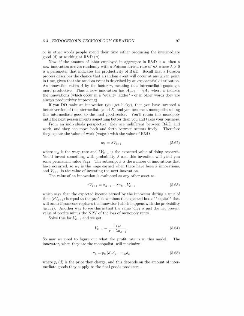
5.3. ENDOGENOUS TECHNOLOGY CREATION 97
or in other words people spend their time either producing the intermediategood (d) or working at R&D (n).Now, if the amount of labor employed in aggregate in R&D is n, then a
new innovation arrives randomly with a Poisson arrival rate of nλ where λ > 0is a parameter that indicates the productivity of R&D. Recall that a Poissonprocess describes the chance that a random event will occur at any given pointin time, given that the random event is described by an exponential distribution.An innovation raises A by the factor γ, meaning that intermediate goods getmore productive. Thus a new innovation has Ak+1 = γAk where k indexesthe innovations (which occur in a "quality ladder" - or in other words they arealways productivity improving).If you DO make an innovation (you get lucky), then you have invented a
better version of the intermediate good X, and you become a monopolist sellingthis intermediate good to the final good sector. You’ll retain this monopolyuntil the next person invents something better than you and takes your business.From an individuals perspective, they are indifferent between R&D and
work, and they can move back and forth between sectors freely. Thereforethey equate the value of work (wages) with the value of R&D
wk = λVk+1 (5.62)
where wk is the wage rate and λVk+1 is the expected value of doing research.You’ll invent something with probability λ and this invention will yield yousome permanent value Vk+1. The subscript k is the number of innovations thathave occurred, so wk is the wage earned when there have been k innovations,and Vk+1 is the value of inventing the next innovation.The value of an innovation is evaluated as any other asset as
rVk+1 = πk+1 − λnk+1Vk+1 (5.63)
which says that the expected income earned by the innovator during a unit oftime (rVk+1) is equal to the proft flow minus the expected loss of "capital" thatwill occur if someone replaces the innovator (which happens with the probabilityλnk+1). Another way to see this is that the value Vk+1 is just the net presentvalue of profits minus the NPV of the loss of monopoly rents.Solve this for Vk+1 and we get
Vk+1 =πk+1
r + λnk+1. (5.64)
So now we need to figure out what the profit rate is in this model. Theinnovator, when they are the monopolist, will maximize
πk = pk (d) dk − wkdk (5.65)
where pt (d) is the price they charge, and this depends on the amount of inter-mediate goods they supply to the final goods producers.
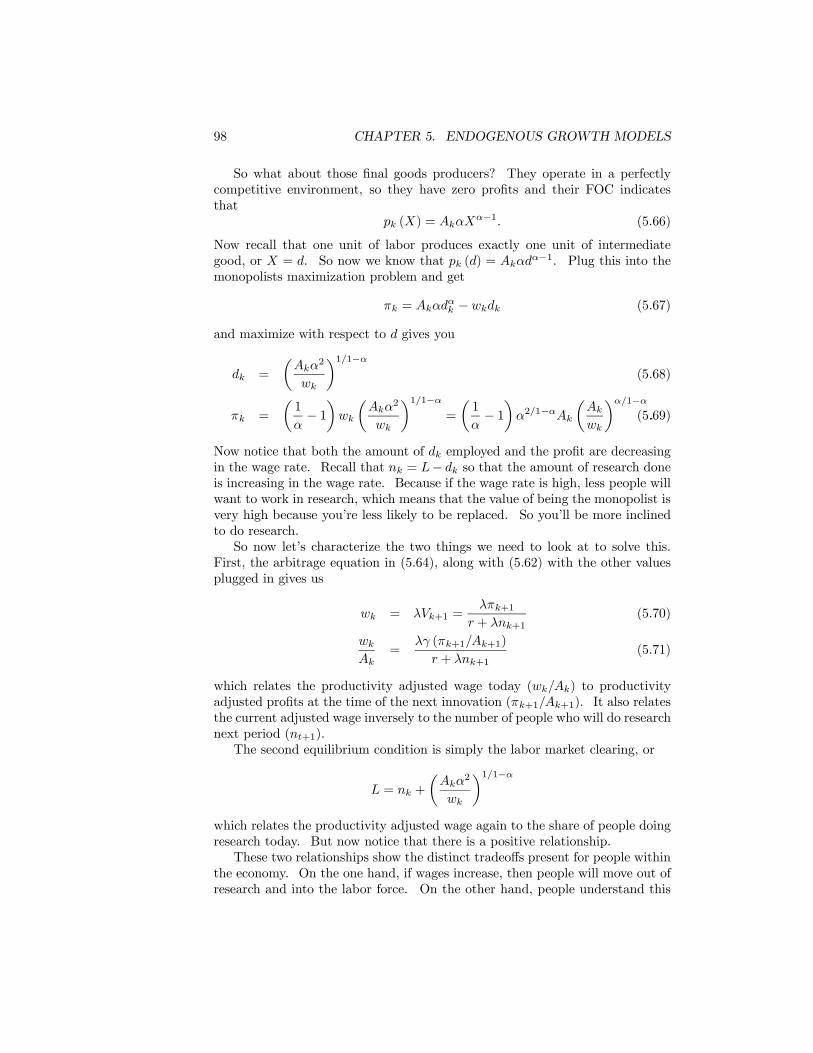
98 CHAPTER 5. ENDOGENOUS GROWTH MODELS
So what about those final goods producers? They operate in a perfectlycompetitive environment, so they have zero profits and their FOC indicatesthat
pk (X) = AkαXα−1. (5.66)
Now recall that one unit of labor produces exactly one unit of intermediategood, or X = d. So now we know that pk (d) = Akαd
α−1. Plug this into themonopolists maximization problem and get
πk = Akαdαk − wkdk (5.67)
and maximize with respect to d gives you
dk =
µAkα
2
wk
¶1/1−α(5.68)
πk =
µ1
α− 1¶wk
µAkα
2
wk
¶1/1−α=
µ1
α− 1¶α2/1−αAk
µAk
wk
¶α/1−α.(5.69)
Now notice that both the amount of dk employed and the profit are decreasingin the wage rate. Recall that nk = L− dk so that the amount of research doneis increasing in the wage rate. Because if the wage rate is high, less people willwant to work in research, which means that the value of being the monopolist isvery high because you’re less likely to be replaced. So you’ll be more inclinedto do research.So now let’s characterize the two things we need to look at to solve this.
First, the arbitrage equation in (5.64), along with (5.62) with the other valuesplugged in gives us
wk = λVk+1 =λπk+1
r + λnk+1(5.70)
wk
Ak=
λγ (πk+1/Ak+1)
r + λnk+1(5.71)
which relates the productivity adjusted wage today (wk/Ak) to productivityadjusted profits at the time of the next innovation (πk+1/Ak+1). It also relatesthe current adjusted wage inversely to the number of people who will do researchnext period (nt+1).The second equilibrium condition is simply the labor market clearing, or
L = nk +
µAkα
2
wk
¶1/1−αwhich relates the productivity adjusted wage again to the share of people doingresearch today. But now notice that there is a positive relationship.These two relationships show the distinct tradeoffs present for people within
the economy. On the one hand, if wages increase, then people will move out ofresearch and into the labor force. On the other hand, people understand this
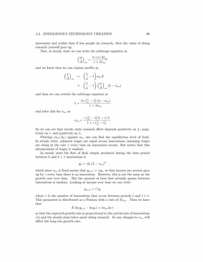
5.3. ENDOGENOUS TECHNOLOGY CREATION 99
movement and realize that if less people do research, then the value of doingresearch yourself goes up.Now, in steady state we can write the arbitrage equation as³w
A
´ss=
λγ (π/A)ssr + λnss
and we know that we can express profits as³ πA
´ss
=
µ1
α− 1¶wkX
=
µ1
α− 1¶³w
A
´ss(L− nss)
and then we can rewrite the arbitrage equation as
1 =λγ¡1α − 1
¢(L− nss)
r + λnss
and solve this for nss as
nss =γ¡1α − 1
¢L− r/λ
1 + γ¡1α − 1
¢ .
So we can see that steady state research effort depends positively on L, nega-tively on r, and positively on λ.Plotting (wk/Ak) against nk, one can find the equilibrium level of both.
In steady state, adjusted wages are equal across innovations (meaning wagesare rising at the rate γ every time an innovation occurs. But notice that thisadvancement of wages is random.In steady state the flow of final output produced during the time period
between k and k + 1 innovations is
yk = Ak (L− nss)α
which since nss is fixed means that yk+1 = γyk, or that income per person goesup by γ every time there is an innovation. However, this is not the same as thegrowth rate over time. But the amount of time that actually passes betweeninnovations is random. Looking at income over time we can write
yt+1 = γεyt
where ε is the number of innovations that occur between periods t and t + 1.This parameter is distributed as a Poisson with a rate of λnss. Then we havethat
E (ln yt+1 − ln yt) = λnss ln γ
or that the expected growth rate is proportional to the arrival rate of innovations(λ) and the steady-state labor spent doing research. So any changes to nss willaffect the long-run growth rate.
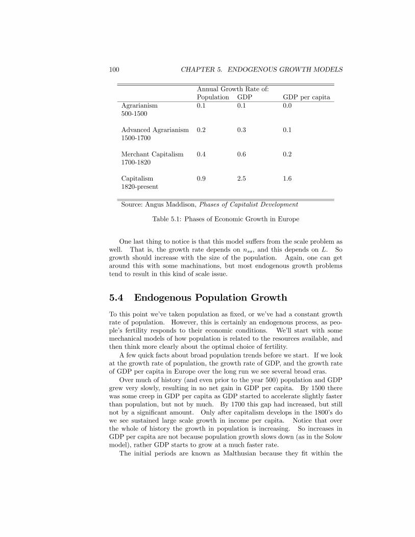
100 CHAPTER 5. ENDOGENOUS GROWTH MODELS
Annual Growth Rate of:Population GDP GDP per capita
Agrarianism 0.1 0.1 0.0500-1500
Advanced Agrarianism 0.2 0.3 0.11500-1700
Merchant Capitalism 0.4 0.6 0.21700-1820
Capitalism 0.9 2.5 1.61820-present
Source: Angus Maddison, Phases of Capitalist Development
Table 5.1: Phases of Economic Growth in Europe
One last thing to notice is that this model suffers from the scale problem aswell. That is, the growth rate depends on nss, and this depends on L. Sogrowth should increase with the size of the population. Again, one can getaround this with some machinations, but most endogenous growth problemstend to result in this kind of scale issue.
5.4 Endogenous Population Growth
To this point we’ve taken population as fixed, or we’ve had a constant growthrate of population. However, this is certainly an endogenous process, as peo-ple’s fertility responds to their economic conditions. We’ll start with somemechanical models of how population is related to the resources available, andthen think more clearly about the optimal choice of fertility.A few quick facts about broad population trends before we start. If we look
at the growth rate of population, the growth rate of GDP, and the growth rateof GDP per capita in Europe over the long run we see several broad eras.Over much of history (and even prior to the year 500) population and GDP
grew very slowly, resulting in no net gain in GDP per capita. By 1500 therewas some creep in GDP per capita as GDP started to accelerate slightly fasterthan population, but not by much. By 1700 this gap had increased, but stillnot by a significant amount. Only after capitalism develops in the 1800’s dowe see sustained large scale growth in income per capita. Notice that overthe whole of history the growth in population is increasing. So increases inGDP per capita are not because population growth slows down (as in the Solowmodel), rather GDP starts to grow at a much faster rate.The initial periods are known as Malthusian because they fit within the
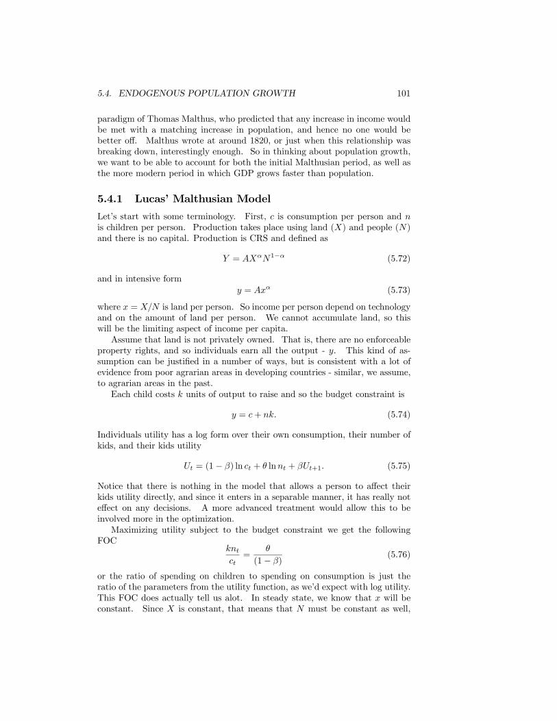
5.4. ENDOGENOUS POPULATION GROWTH 101
paradigm of Thomas Malthus, who predicted that any increase in income wouldbe met with a matching increase in population, and hence no one would bebetter off. Malthus wrote at around 1820, or just when this relationship wasbreaking down, interestingly enough. So in thinking about population growth,we want to be able to account for both the initial Malthusian period, as well asthe more modern period in which GDP grows faster than population.
5.4.1 Lucas’ Malthusian Model
Let’s start with some terminology. First, c is consumption per person and nis children per person. Production takes place using land (X) and people (N)and there is no capital. Production is CRS and defined as
Y = AXαN1−α (5.72)
and in intensive formy = Axα (5.73)
where x = X/N is land per person. So income per person depend on technologyand on the amount of land per person. We cannot accumulate land, so thiswill be the limiting aspect of income per capita.Assume that land is not privately owned. That is, there are no enforceable
property rights, and so individuals earn all the output - y. This kind of as-sumption can be justified in a number of ways, but is consistent with a lot ofevidence from poor agrarian areas in developing countries - similar, we assume,to agrarian areas in the past.Each child costs k units of output to raise and so the budget constraint is
y = c+ nk. (5.74)
Individuals utility has a log form over their own consumption, their number ofkids, and their kids utility
Ut = (1− β) ln ct + θ lnnt + βUt+1. (5.75)
Notice that there is nothing in the model that allows a person to affect theirkids utility directly, and since it enters in a separable manner, it has really noteffect on any decisions. A more advanced treatment would allow this to beinvolved more in the optimization.Maximizing utility subject to the budget constraint we get the following
FOCkntct
=θ
(1− β)(5.76)
or the ratio of spending on children to spending on consumption is just theratio of the parameters from the utility function, as we’d expect with log utility.This FOC does actually tell us alot. In steady state, we know that x will beconstant. Since X is constant, that means that N must be constant as well,
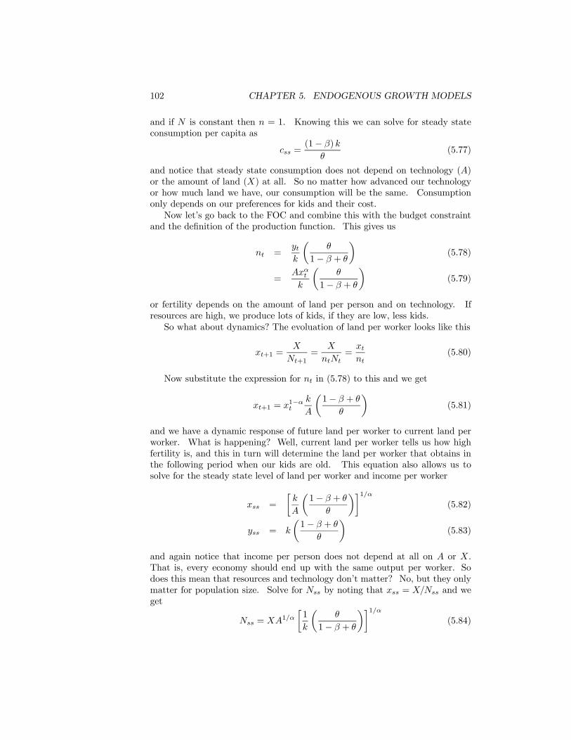
102 CHAPTER 5. ENDOGENOUS GROWTH MODELS
and if N is constant then n = 1. Knowing this we can solve for steady stateconsumption per capita as
css =(1− β) k
θ(5.77)
and notice that steady state consumption does not depend on technology (A)or the amount of land (X) at all. So no matter how advanced our technologyor how much land we have, our consumption will be the same. Consumptiononly depends on our preferences for kids and their cost.Now let’s go back to the FOC and combine this with the budget constraint
and the definition of the production function. This gives us
nt =ytk
µθ
1− β + θ
¶(5.78)
=Axαtk
µθ
1− β + θ
¶(5.79)
or fertility depends on the amount of land per person and on technology. Ifresources are high, we produce lots of kids, if they are low, less kids.So what about dynamics? The evoluation of land per worker looks like this
xt+1 =X
Nt+1=
X
ntNt=
xtnt
(5.80)
Now substitute the expression for nt in (5.78) to this and we get
xt+1 = x1−αt
k
A
µ1− β + θ
θ
¶(5.81)
and we have a dynamic response of future land per worker to current land perworker. What is happening? Well, current land per worker tells us how highfertility is, and this in turn will determine the land per worker that obtains inthe following period when our kids are old. This equation also allows us tosolve for the steady state level of land per worker and income per worker
xss =
∙k
A
µ1− β + θ
θ
¶¸1/α(5.82)
yss = k
µ1− β + θ
θ
¶(5.83)
and again notice that income per person does not depend at all on A or X.That is, every economy should end up with the same output per worker. Sodoes this mean that resources and technology don’t matter? No, but they onlymatter for population size. Solve for Nss by noting that xss = X/Nss and weget
Nss = XA1/α∙1
k
µθ
1− β + θ
¶¸1/α(5.84)
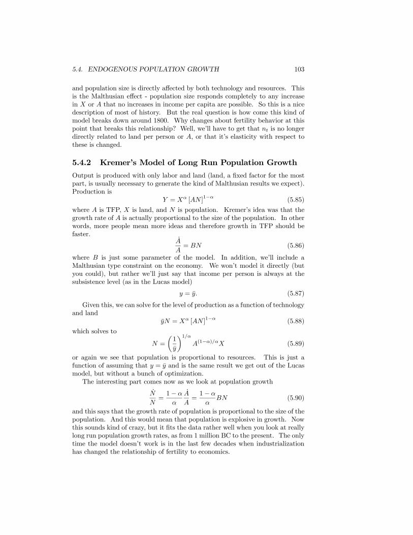
5.4. ENDOGENOUS POPULATION GROWTH 103
and population size is directly affected by both technology and resources. Thisis the Malthusian effect - population size responds completely to any increasein X or A that no increases in income per capita are possible. So this is a nicedescription of most of history. But the real question is how come this kind ofmodel breaks down around 1800. Why changes about fertility behavior at thispoint that breaks this relationship? Well, we’ll have to get that nt is no longerdirectly related to land per person or A, or that it’s elasticity with respect tothese is changed.
5.4.2 Kremer’s Model of Long Run Population Growth
Output is produced with only labor and land (land, a fixed factor for the mostpart, is usually necessary to generate the kind of Malthusian results we expect).Production is
Y = Xα [AN ]1−α (5.85)
where A is TFP, X is land, and N is population. Kremer’s idea was that thegrowth rate of A is actually proportional to the size of the population. In otherwords, more people mean more ideas and therefore growth in TFP should befaster.
A
A= BN (5.86)
where B is just some parameter of the model. In addition, we’ll include aMalthusian type constraint on the economy. We won’t model it directly (butyou could), but rather we’ll just say that income per person is always at thesubsistence level (as in the Lucas model)
y = y. (5.87)
Given this, we can solve for the level of production as a function of technologyand land
yN = Xα [AN ]1−α (5.88)
which solves to
N =
µ1
y
¶1/αA(1−α)/αX (5.89)
or again we see that population is proportional to resources. This is just afunction of assuming that y = y and is the same result we get out of the Lucasmodel, but without a bunch of optimization.The interesting part comes now as we look at population growth
N
N=1− α
α
A
A=1− α
αBN (5.90)
and this says that the growth rate of population is proportional to the size of thepopulation. And this would mean that population is explosive in growth. Nowthis sounds kind of crazy, but it fits the data rather well when you look at reallylong run population growth rates, as from 1 million BC to the present. The onlytime the model doesn’t work is in the last few decades when industrializationhas changed the relationship of fertility to economics.
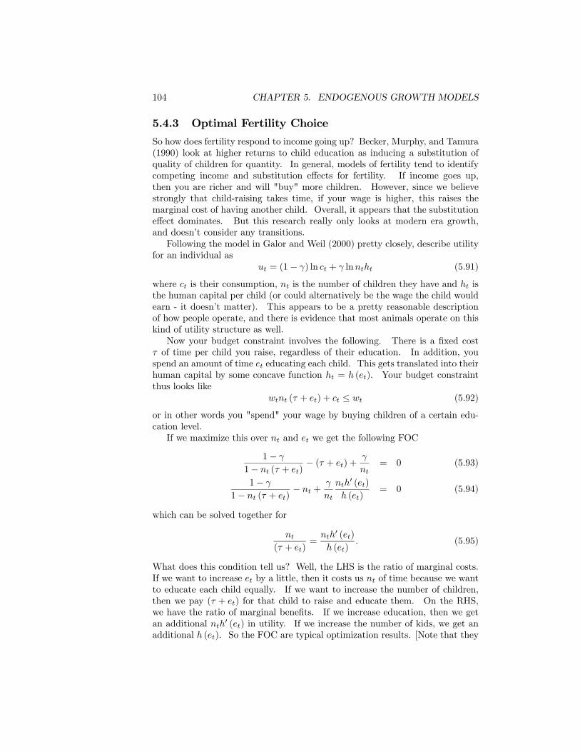
104 CHAPTER 5. ENDOGENOUS GROWTH MODELS
5.4.3 Optimal Fertility Choice
So how does fertility respond to income going up? Becker, Murphy, and Tamura(1990) look at higher returns to child education as inducing a substitution ofquality of children for quantity. In general, models of fertility tend to identifycompeting income and substitution effects for fertility. If income goes up,then you are richer and will "buy" more children. However, since we believestrongly that child-raising takes time, if your wage is higher, this raises themarginal cost of having another child. Overall, it appears that the substitutioneffect dominates. But this research really only looks at modern era growth,and doesn’t consider any transitions.Following the model in Galor and Weil (2000) pretty closely, describe utility
for an individual asut = (1− γ) ln ct + γ lnntht (5.91)
where ct is their consumption, nt is the number of children they have and ht isthe human capital per child (or could alternatively be the wage the child wouldearn - it doesn’t matter). This appears to be a pretty reasonable descriptionof how people operate, and there is evidence that most animals operate on thiskind of utility structure as well.Now your budget constraint involves the following. There is a fixed cost
τ of time per child you raise, regardless of their education. In addition, youspend an amount of time et educating each child. This gets translated into theirhuman capital by some concave function ht = h (et). Your budget constraintthus looks like
wtnt (τ + et) + ct ≤ wt (5.92)
or in other words you "spend" your wage by buying children of a certain edu-cation level.If we maximize this over nt and et we get the following FOC
1− γ
1− nt (τ + et)− (τ + et) +
γ
nt= 0 (5.93)
1− γ
1− nt (τ + et)− nt +
γ
nt
nth0 (et)
h (et)= 0 (5.94)
which can be solved together for
nt(τ + et)
=nth
0 (et)
h (et). (5.95)
What does this condition tell us? Well, the LHS is the ratio of marginal costs.If we want to increase et by a little, then it costs us nt of time because we wantto educate each child equally. If we want to increase the number of children,then we pay (τ + et) for that child to raise and educate them. On the RHS,we have the ratio of marginal benefits. If we increase education, then we getan additional nth0 (et) in utility. If we increase the number of kids, we get anadditional h (et). So the FOC are typical optimization results. [Note that they
5.4. ENDOGENOUS POPULATION GROWTH 105
don’t depend on γ either, this is just the decision about how to allocate ourchild-raising time to quantity and quality].Let’s think about what happens when the returns to education change. That
is, h (et) shifts up, but the shape of it (h0 (et)) doesn’t change. (All years ofschooling now give you more human capital, but the amount you gain from oneadditional year hasn’t changed). Then the marginal benefit of all children hasgone up relative to the marginal benefit of education. So the answer to equatingthis situation is to lower the number of kids, and raise the amount of education.So to account for the intertwined drop in fertility and rise in education, we needsomething to push up h (et).This FOC, though, doesn’t offer us any situation in which the wage matters.
That is, there is no effect of parent wage on fertility, and in particular wecannot see how fertility would go up with income, as in a Malthusian world.So this model is "modern" in that it captures the quantity quality tradeoff, butnot Malthusian. To add a Malthusian element, we need simply establish asubsistence constraint. That is, there is a minimum level of consumption c thatpeople must consume at all times.
ct = wt [1− nt (τ + et)] ≥ c (5.96)
so we need to evaluate this somehow. First, go back to the utility function.Note that we have CD preferences, and we know that with these, we spend aconstant fraction of our wealth on each "good". In our case, we would like tospend the fraction (1− γ) of our wealth, wt, on consumption. Since we haveone unit of time, that means that we must spend (1− γ) of our time working,leaving γ of our time for raising kids. So we know that nt (τ + et) = γ, whenwe are unconstrained. Plug this in above and we get that
ct = wt [1− γ] ≥ c (5.97)
So if wt > c/ (1− γ), then we are unconstrained by subsistence. However, ifwt < c/ (1− γ) then we are constrained. Now, wt [1− nt (τ + et)] = c binds,and this dictates that share of our time spent raising children nt (τ + et) =1− c/wt. If wt is very low, then this number goes to zero. In other words, if weare very poor, then we spend very little time on having kids (regardless of theireducation level). To see this, imagine that et = 0. Then nt = (1− c/wt) /τ .So if wt were to rise, so would fertility. The subsistence constraint deliversthe result that at low incomes, rising income leads to higher fertility. Once weget to a cutoff of wt = c/ (1− γ), then the time spent no longer increases (butmight be allocated differently).Draw the diagram showing time on children on y-axis and c on the x-axis.
At subsistence, vertical until γ and then horizontal. As wages increase, thebudget line rotates out from a point on the y-axis equal to one.So with these mechanisms in place, what can we say about how fertility
evolves with income? Well, if wages increase, at first the time spent on childrenincreases and then flattens out. So we can get a Malthusian result, but nothingthat necessarily drives a quality quantity tradeoff. For that we have to make
106 CHAPTER 5. ENDOGENOUS GROWTH MODELS
further assumptions about how wages and human capital evolve. Using ourFOC we will have
h (et)− (τ + et)h0 (et) = 0 if et > 0 (5.98)
h (et)− (τ + et)h0 (et) > 0 if et = 0 (5.99)
which just involves the condition that et ≥ 0 (i.e. you can’t uneducate yourchildren). So if it turns out that you’ll fail to educate your children if thereturn on education isn’t high enough to overcome the cost of adding additionaleducation.What does our fertility regime tell us about education? Well, let’s look back
at the FOC for education, which if rearranged says that
1− γ
γ
nt (τ + et)
1− nt (τ + et)=
h0 (et) (τ + et)
h (et). (5.100)
Look back at the fertility decision, which if we are not at subsistence requiresthat nt (τ + et) = γ and so this whole equation balances nicely. In other wordswhen the subsistence constraint does not bite, all our FOC conditions hold, andwe have positive education (as h0 (et) (τ + et) = h (et)). However, when thesubsistence constraint does bite with low wages, we have that nt (τ + et) < γand this then implies that h0 (et) (τ + et) < h (et) and this is what we alreadyknow implies that et = 0. So what we have found is that when the subsistenceconstraints bind, we fail to educate our children. Why? We have very littletime to devote to kids, and this is taken up with the fixed time cost of children,so to maximize utility we have lots of uneducated kids. Once we have wageshigh enough, we actually achieve positive et.
Appendix A
Solutions
A.1 Solving for actual consumption (Example4)
Using the expression for the path of consumption, we can solve for actual con-sumption by period by using the expected value budget constraint that holdsat time t
E
"T−1Xs=t
Cs
#= E
"T−1Xs=t
Ys
#+At.
and notice the subscripts. What we are saying here is that the expected valueof future consumption (from today until period T − 1) must equal the expectedvalue of income over that same period plus the level of assets you have on handat period t. So is there some way to evaluate the expectations? There is, andlet’s start with the expectation of income first.
E
"T−1Xs=t
Ys
#= Yt +E
"T−1Xs=t
Ys+1
#
= Yt +E
"T−1Xs=t
Ys + εs+1
#
= Yt +T−1Xs=t
E (Ys) +T−1Xs=t
E (εs+1)
= Yt + (T − 1− t)Yt + 0
= Yt (T − t)
where the final line follows because our expectation of all the transitory shocksto income is just zero. Now we can look at the expectation of consumption,where we want to try and get Cs in terms of Ct. Look first at the following
E (Ct+1) = Ct + ασ2/2
107
108 APPENDIX A. SOLUTIONS
which follows from our expression for the optimal consumption path. Iteratethis forward and you’ll find
E (Cs) = Ct +¡ασ2/2
¢(s− t) +
T−1Xs=t
E (εs+1)
= Ct +¡ασ2/2
¢(s− t)
where again we’ve used the fact that the expected value of the transitory shocksis equal to zero. Now, we can plug this into the summation of expected con-sumption
E
"T−1Xs=t
Cs
#=
T−1Xs=t
Ct +¡ασ2/2
¢(s− t)
which can be evaluated as
E
"T−1Xs=t
Cs
#= (T − t)Ct +
(T − t− 1) (T − t)
2
ασ2
2.
We now can fill in all the pieces of our expected budget constraint, which is now
(T − t)Ct +(T − t− 1) (T − t)
2
ασ2
2= At + Yt (T − t)
and can be rearranged to be
Ct =At
T − t+ Yt −
(T − t− 1)ασ24
and this gives us exactly what consumption will be in any period t. Note thatwe can’t actually specify what At is because it depends on the actual realizationsof the transitory shocks. But given some level of At, this is how we should act.
A.2 Consumption Path in the Stochastic Ram-sey Model
The answer to the following first order condition
1
ct=
1
1 + θE
∙1 + αAt+1k
αt+1 − δ
ct+1
¸involves using the inelegantly named "guess and verify" method. It’s know thatproblems that have log utility tend to have linear relationships of consumptionand income. So we guess that consumption is of the form
ct = βAtkαt
A.3. SOCIAL SECURITY IN THE OLG MODEL (EXAMPLE 17) 109
but we don’t know what β is, or whether in fact this really will work. So weplug this in to the first order condition to see if we can make it work.
1
βAtkαt=
1
1 + θE
∙α
βkt+1
¸.
We know how kt+1 evolves under our suggested rule of consumption, or kt+1 =(1− δ) kt + (1− β)Atk
αt so we have
1
βAtkαt=
1
1 + θE
∙α
β (1− β)Atkαt
¸and we can do some algebra, and then evaluate the expectation which is nowall in terms of stuff we know.
1− β =α
1 + θ
This means that if we set β = 1− α1+θ , then it must be the case that our FOC
holds. So we say that
ct =
µ1− α
1 + θ
¶Atk
αt .
A.3 Social Security in the OLG Model (Exam-ple 17)
We showed that the evolution of the capital stock with social security was
kt+1 =(1− α)
(1 + n) (2 + θ)kαt −
d
1 + n
∙1 + θ
2 + θ
∙n+ δ − αkα−1t
1 + αkα−1t − δ
¸+ 1
¸and then asserted that this had kt+1 less than it would be in the non-socialsecurity world. This is the same as saying that the second term above ispositive. When is
d
1 + n
∙1 + θ
2 + θ
∙n+ δ − αkα−1t
1 + αkα−1t − δ
¸+ 1
¸> 0.
This is the same as asking if
1 + θ
2 + θ
∙n− r
1 + r
¸> −1
which can be solved to show that
n > −2 + θ
1 + θ(1 + r) + r
> r
µ−11 + θ
¶− 2 + θ
1 + θ
or that n is non-negative, and if it is negative, is can only be slightly negative.Since n > 0 almost everywhere and at all times, this seems like it is satisfied.

110 APPENDIX A. SOLUTIONS
Appendix B
Problems
B.1 Consumption/Savings1. Gertrude lives for two periods. In the first period she earns a wage of 100.In the second period her wage is zero. She earns interest on her savingsof r > 0. Her utility is U = c1−σ/1− σ and she has a zero discount rate.For what values of σ will her first period consumption be equal to 50?For what values will it be less than 50? For what values will it be exactlyequal to 50?
2. Let’s say your utility function is U = x3. If you live for two periods andhave $300 to allocative across those two periods, what is your optimalstrategy? Now, let’s say you are offered either $150 or a chance to flipa coin for either $100 or $200 - which do you choose? What property ofyour utility function determines these choices?
3. Calculate the intertemporal elasticity of substitution for a CRRA utilityfunction. The intertemporal elasticity is defined as
∂ (c2/c1)
∂ (1 + r)
(1 + r)
c2/c1. (B.1)
4. Consider a two-period Fisher model in which utility in each period isCRRA. Wages are equal to W in each period. Solve for the derivative offirst period savings with respect to the interest rate: ∂S/∂r. For whatvalues of σ is the sign of ∂S/∂r always negative? What are the conditionsunder which ∂S/∂r is positive?
5. Set up the Lagrangian for a two period Fisher model with wages equalto W1 and W2, a discount rate of θ, and an interest rate of r. Solve forthe Euler equation relating consumption in period 1 and period 2. Doesthe relationship of consumption between period 1 and period 2 dependon a) the size of wages or b) the distribution of wages? Now imagine
111
112 APPENDIX B. PROBLEMS
that person lives in a world with no financial system, so that they cannotsave or borrow at all. They have to consume exactly their wages in eachperiod. Solve for the interest rate that makes this the optimal outcome inthe Fisher model. How does this interest rate you just solved for changewith the ratio of W2/W1?
6. This is a two period model. Anyone can borrow at the rate rb = 1(100% interest) and anyone can save at the rate rs = 0. Their prefer-ences are given by V = ln c1 + ln c2. Find optimal consumption for thefollowing individuals who have different wage profiles in their life. A) Mr.Pink has w1 = 32 and w2 = 32, B) Mr. White has w1 = 0 and w2 = 64,C) Mr. Orange has w1 = 24 and w2 = 40. Who has the highest lifetimeutility?
7. Danny lives for two periods. In the first period he has an income of X. Inthe second period he has an income of zero. He can save money at a realinterest rate of zero, but he cannot borrow. He is born with zero assetsand dies with zero assets. He has log utility and his time discount rate iszero. There is a government program with the following rules: if the sumof your income and your savings in any period is less than some level M ,then the government will give you enough money so that you can consumeM . If the sum of your income and savings in a period is greater thanM , then the government gives you nothing. Describe the relationshipbetween Danny’s first period savings rate (S/X) and X. If you can’t getan exact solution, draw a picture and discuss what the solution might looklike.
8. Rusty will live for two periods with certainty, and he’ll live for a thirdperiod with probability 50%. He’ll find out at the end of period one (thatis, after he’s done his first period consumption) whether he’ll die at theend of period two or period three. He has earning of one in the first period,and no income after that. Rusty has CRRA utility, a time discount rate ofzero, and faces an interest rate of zero. He can’t die in debt. A) Derivethe equation you’d solve to get Rusty’s optimal first period consumption- you don’t actually have to solve it out. B) A government programis introduced that takes away T in takes from every worker in the firstperiod and pays 2T to all people who survive into the third period of life.What is the value of T that maximizes Rusty’s utility? (You don’t haveto use algebra for this, you can actually just reason out the answer).
9. Tess lives for two periods and in the first period she has income of 8 dollars.In the second period her income is either 0 or 8, each with probability of50%. The interest rate is zero. Her utility is quadratic, U = c − 0.05c2and she has a discount rate of zero. Tess can take a test that will tell herwhat her second period income will be, and she can take this test prior toconsuming in the first period. If she does not take the test, she will notknow her second period income until after the first period is over. Thetest costs 2 dollars. Calculate whether Tess should take the test or not.
B.1. CONSUMPTION/SAVINGS 113
10. This is a two period model in which people work in both periods. Theystart with no assets and die with no assets. They can borrow and lendat r = 0, and their θ = 0. Everyone has log utility. In the first period,everyone earns $10. In the second period half the people earn $15 andhalf make $5. In the first period, no one knows which group they belongto. A) The government is considering cutting taxes by $1 per person inthe first period (raising income to $11) and increasing taxes in the secondperiod to pay back the debt (which amounts to $1 per person). Taxesin the second period can either be lump sum of $1 per person or can beproportional to 10% of each persons income in the second period. Howdoes each of these tax plans affect utility and the national savings rate(that is, total savings divided by total income). B) A test is inventedthat will tell people at the beginning of period 1 what their income inperiod 2 will be. How would the availability of this test affect utility?How would it affect savings?
11. This problem is about certainty equivalence. Ty has quadratic utility ofU = β0 + β1c− β2c
2. He is a simple man. He lives only one period andso he consumes everything he earns in that one period. A) First, assumeTy has certain income of $15 and calculate his total utility and marginalutility of consumption. B) Now assume Ty receives either $10 or $20 withprobability 50%. Again calculate his total utility and marginal utility. C)In which situation is total utility higher? In which situation is marginalutility higher? D) Now Ty lives for two periods. In the first period he gets$15 with certainty. Will his savings behavior in the first period dependon whether his second period income is $15 with certainty or is $10/$20with 50%? Explain.
12. Consider a one-period model in which individuals make a labor/leisuredecision. Individuals have one unit of time. Utility is U = lnn+c1−σ/1−σwhere n is leisure and c is consumption. People take the wage w as given.They live only one period. They earn (1− n)w and consume all theirearnings. Show how the effect of the wage on labor supply depends on thevalue of σ. For what values will an increase in the wage have a positiveeffect on labor supply, and for what values will the effect be negative?
13. Take the usual intertemporal optimization problem over consumption andleisure. Variation in consumption and leisure can be caused by two things:variation in the interest rate or variation in the real wage. For which ofthese two causes will consumption and leisure be positively correlated andfor which will they be negatively correlated? Explain.
14. Take a model where individuals live for two periods. Utility is U = ln c1+ln c2 + lnn1 + lnn2. Eac individual has one unit of time. There are twotypes of individuals. Some earn a wage of 1 in the first period and 2 inthe second. The others earn 2 in the first period and 1 in the second.Individuals cannot borrow, but that can save at an interest rate of zero.
114 APPENDIX B. PROBLEMS
Individuals are born with zero assets and die with zero assets. A) Withoutdoing any math, which type of person is likely to have more variation inactual earnings (w (1− n)) between periods? B) Calculate total earnings(w (1− n)) in each period for each type of person. Does this match yourintuition from part A?
15. A person may live for one, two, or three periods. At the end of period one,there is a 50% chance he will die, and a 50% chance he lives in the secondperiod. If he does live to the second period, then at the end of period 2there is a 50% chance of living into the 3rd period and a 50% chance ofdying. His wealth at the beginning of period 1 is A, and he earns no wageincome. The interest rate and discount rate are both equal to zero. Hehas log utility. Solve for his optimal consumption plan.
16. People live for two periods and wish to maximize their lifetime utility ofU = ln c1 + ln c2. They have a zero discount rate and face a positiveinterest rate r. They have two options for their time. They can work orthey can go to school. The time spent in school is n and the time spentworking is (1− n). Time spent in school creates human capital next periodaccording to the formula ht+1 = (ntht)
αx1−α where x represents public
education spending. Note that human capital in period t+ 1 depends onyour human capital in period t. Individuals are endowed with a valueof h1 which can be thought of as innate ability. Income depends on thebase wage, human capital, and time working as yt = wht (1− nt). Thebase wage rate w is fixed. A) Assuming individuals can borrow and lendfreely, what is the optimal choice of education over time (n1, n2)? B)Now assume that individuals are financially constrained and can neitherborrow nor lend. Now what is the optimal choice of education over time?C) The government is planning on raising education spending (increasingx). Compare the effect of this plan in both financial situations on timespent on education and on second period income. D) Do high abilityindividuals (those with large h1) gain more second period income fromthe increase in x in either financial situation? Does this tell you anythingabout how education spending influences inequality within the economy?
17. Consider an economy that lasts for two periods, and is made up of twogenerations. The partents live only in the first period and the childrenlive only in the second period. A family is composed of one parent andone child (and don’t worry that they aren’t alive at the same time). Thereis also a government, which exists for both periods. The interest rate isexogenous and equal to zero. People in the first period receive a beforetax income of y1 and people in the second period earn a before tax incomeof y2. The government can impose lump-sum taxes (or transfers) of t1and t2. The government could also levy a proportional inheritance tax, atrate tb: if the size of bequests left is b, then the tax collected will be tbb.The government faces the same interest rate (zero) as the people. It doesnot do any spending other than on transfers. The government must have
B.1. CONSUMPTION/SAVINGS 115
a balanced budget over the two periods, so t1+ tx+ tbb = 0. A) Considerthe case where a familiy has the utility function U = ln c1 + ln c2 wherethe subscripts refer to the generations. The tax on bequests, tb, is equalto zero. Calculate the size of bequests left as a function of y1, y2 and t.B) what happens to the size of bequests left if the government raises firstperiod taxes by some amount d? C) Does Ricardian equivalence hold?(That is, does the pattern of consumption change due to this tax increase).D) Now suppose everything is the same, except that tb is positive and lessthan one. Assume that the government sets taxes in period two so thatis budget is balanced given taxes in period one aside plus any inheritancetaxes collected. But not that second period taxes are exogenous fromthe perspective of families. Now, what is the size of bequests, and whathappens if first period taxes go up by d? Now, does Ricardian equivalencehold?
18. A man has a potential lifespan of 100 years. For the first 50, he lives withcertainty. After the 50th year, he will enter a battle, and there is a 50%chance that he will survive. If he survives the he will live with certaintyfor another 50 years. At birth he has $100, and does not earn any otherwages. He cannot die in debt. He has log utility, and the interest rate anddiscount rate are both zero. Solve for initial consumption.
19. Madeline lives for two periods. In each period she earns income of 1. Herutility is U = ln c1 + ln c2. She can borrow or lend some asset betweenperiods 1 and 2 that has a real interest rate of zero. However, thereis a 50% chancee that between periods 1 and 2 all debts and financialwealth will be wiped out. That is, if she borrows, there is a 50% chancethat she will not have to pay back the loan, and if she saves, there is a50% chance that all her savings will disappear. Solve for her optimal firstperiod consumption.
20. Nicole lives for two periods. In the first period she has income of 3. Inthe second period she will have income of zero. The interest rate andthe time discount rate are both zero. She cannot borrow and her utilityfunction is U = ln c1 + ln c2. There is a government welfare programthat provides a consumption floor of cmin in the second period. In otherwords: if she does not have enough money left over to afford to consumecmin, then the government will give her enough money so that she canafford it. A) Obviously, for high enough values of cmin Nicole will spendall her income in the first period and just consume cmin in the second.For low enough levels of cmin she will act as if the program did not exist.Calculate the critical level of cmin at which she is indifferent between thesetwo strategies. B) Now suppose there is only a 50% chance she’ll be alivein the second period. Now calculate the critical value of cmin.
21. Assume that the following facts are true. 1) OVer the long term ,thereal wage has risen dramatically. 2) Over the long term, the fraction of
116 APPENDIX B. PROBLEMS
their time that people spend working has remained constant, and 3) overthe long term the ratio of per capita consumption to the real wage hasremained constant. Assuming that utility is given by
U =c1−σt
1− σ+ β
n1−γt
1− γ. (B.2)
Based on the three facts, what can you conclude about the value of σ?
B.2 Mechanical Growth1. Output per worker is 5 times higher in country A as in country B. Assum-ing that the countries have identical Cobb-Douglas production functions,and that capital’s share is 1/3, by what factor does MPK differe betweenthe countries. What if capital’s share is 2/3?
2. The production function is y = k1/2. Suppose that capital per worker is400. The savings rate is 50%. The depreciation rate is 5%. There is nopopulation growth or technical change. A) Is the country at its steadystate of output per capita, above its steady state, or below its steadystate? B) Now suppose there is a large immigration into the country. Thepopulation quadruples. The new immigrants do not bring any new capitalwith them. Following the immigration is output per capita above, below,or at the steady state? C) What is the growth rate of income per capitaimmediately after the immigration?
3. There are two countries, A and B, each described by the Solow model.In both, the production function is k1/2, and the depreciation rate is0.02. There is no technological change. In A, the savings rates i 0.2,and population growth is zero. In country B the savings rate is 0.4 andpopulation growth is 0.02. Both countries are observed to have incomeper capita of 5 at time zero. Draw a graph with time on the horizontalaxis and income per capita on the vertical axis showing how the level ofincome per capita in the two countries will evolve over time.
4. Consider a Solow model with positive rates of population growth, depreci-ation, and technological change. Imagine a country is in steady state, andsuddenly its rate of technological change increases. Describe how outputper efficiency unit evolves over time. Describe how output per personevolves over time. If you have trouble with the math, draw the graphs.
5. Two countries are described by the Solow model with y = k1/2. In both,n+δ = 0.1. In country A, s = 0.1 while in country B, savings are a functionof the capital stock, s = 0.2
³1
1+k
´. A) Show that the two countries have
the same steady state, B) Solve for the growth rate of income per person.If both countries start with the same stock of capital per person, whichcountry will grow faster? Will this country always grow faster?
B.2. MECHANICAL GROWTH 117
6. Consider a Solow model in which the growth rate of population is endoge-nous. Specifically
n =
⎧⎨⎩ nh if y < y
nl if y ≥ y(B.3)
where nh > nl. Production is y = kα. Capital depreciates at δ and thereis no technological change. The savings rate is exogenous. A) Draw graphsshowing the different possible configurations of the steady state values ofcapital per person (i.e. single steady states, multiple steady states) andlable each steady state as stable or unstable. B) For what values ofthe savings rate with the model display multiple steady states? For whatvalues will there be a single steady state?
7. Consider an economy with two kinds of capital. k is private capital, andz is government capital (highways, ports, dams, etc.). The productionfunction is y = k1/3z1/3. Both types of capital depreciate at the rate δ.There is no population growth or technological change. The governmentcollects a fraction, τ , of output that it uses to build new governmentcapital. Of the remaining output, s is saved to invest in building newprivate capital. A) Write down the equations of motion for k and z. B)Solve for the steady state values of k, z, y. C) What rate of taxationmaximizes income per capita in the steady state?
8. Consider a country with a production function of y = kα. Populationgrows at the rate n and capital depreciates at the rate δ. There is no tech-nological change. Consumption is each to a constant fraction of output,denoted c. In addition, every period a payment in the amount of p percapita must be made to the foreign power which provides protection forthis country. All output that is not consumed or paid to the foreign poweris invested. A) Write down the differential equation governing the evolu-tion of the per capita stock of capital in this country. B) Draw the Solowdiagram for this country. Is there more than one equilibrium level of thecapital stock and of output? Is so, identify all the equilibria. Indicate thedynamics on the diagram - that is, show to which equilibria an economywill move given it’s initial stock of capital per person.
9. An economy is described by the Solow model with y = k1/2, and somevalues of n and δ. Currently the savings rate is 0.6, and the country isat its steady state. Two course of action are proposed. One is to lowersavings to 0.5, and the other is to lower savings to 0.4. Graphs the pathsof consumption per capita over time following the introduction of eachpolicy, and show how these consumption levels compare to consumptionin the old steady state. Explain.
10. Two countries are described by the Solow model and have the same savingsrates, the same values of n,δ, and g but differ in their technology. A1 6= A2and their production functions are y1 = A1k
α1 and y2 = A2k
α2 . Both
118 APPENDIX B. PROBLEMS
countries are in steady state. A) By what factor do the two countriescapital stocks differ? B) By what factor do the two countries values of Adiffer? C) By what factors do the two countries MPKs differ?e
11. A country has the production function Y = A (bK)α (cL)1−α and thegrowth rate of A is gA, the growth rate of b is gb and the growth rate of cis gc. Population growth is zero. Calculate the growth rate of output percapita in the steady state of a Solow model.
12. There are two countries described by the Solow model. They both havethe same savings rates, population growth rates, and depreciation rates.There is no technological change. The production function in both isy = kα. In country 1 there is a proportional tax rate of τ on income.Savings is done from post-tax income. In country 2 there is constant percapita tax of Ψ per person. Savings is done out of post-tax income. Thesize of the per person tax Ψ is set so that taxes per person are equal tothose collected in steady state by the country with the proportional tax.A) Solve for Ψ. B) Describe the dynamics of the two economies. Showthat there are different possible configurations of steady states in country2 relative to country 1. C) Show how the different configurations of steadystates in 2 relative to 1 depend on the parameters. Derive the cases inwhich each possible configuratino will occur.
13. Two countries have production functions of y = k1/3h1/3 and physical andhuman capital are accumulated according to
k = sky − (n+ δ) k
h = shy − (n+ δ)h.
Two countries have the same levels of sk, but differ by a factor of two inthe size of sh. By what factor will their steady state levels of output perworker differ?
B.3 Dynamic Optimization1. Rodney lives for 40 periods. He has CARA utility, or U = − (1/α) e−αc.He earns 100 dollars in each period, and the interest rate is r and thediscount rate is θ. He has zero assets when he is born and will die with zeroassets, but Rodney can borrow and save during his lifetime. A) Derivethe FOC relating consumption in adjacent periods of life. B) Assume thatα = 1, θ = 0.05, r = 0 and derive optimal first period consumption. You’llhave to use the approximation that ln (1 + x) = x which holds for valuesof x close to zero.
2. Consider the optimal consumption path of Abigail, who will live exactly Tperiods. In the first period, she has earnings of one dollar. Subsequently,her earnings grows at the rate g in each period, so that second period
B.3. DYNAMIC OPTIMIZATION 119
wages are (1 + g), third period wages are (1 + g)2, and so on. Abigail
can borrow and lend freely at an interest rate of zero, and she has a zerodiscount rate. Her utility is CRRA. She starts life with zero assets anddies with zero assets. Calculate her optimal savings in the first period oflife. What is the effect of increasing g on her first period saving. Explain.
3. Crockett and Tubbs have the same preferences (they have identical utilityfunctions and identical discount rates). Both are born at time zero anddie (with certainty) at time T . Both face the same interest rate. Eachis born with zero assets and dies with zero assets. Both are liquidityconstrained: they are never allowed to have negative assets. They havedifferent lifetime wage paths. There is no uncertainty, and both Crockettand Tubbs know exactly, in advance, their entire path of wages over theirlife. You observe Crockett’s consumption growing at a constant, positiverate over his life, while Tubbs’ consumption declines at a constant rateover his life. The rate at which Tubbs’ consumption declines is smallerthan the rate at which Crockett’s consumption rises. However, the presentdiscounted value of their lifetime consumption is identical. Which manhas higher lifetime utility? Explain.
4. Lacy has wealth of A at time zero, and she will live infinitely, but she willnot earn any income in her life. The interest rate is zero. She is unableto borrow. She has log utility with some discount rate θ > 0. Time iscontinuous. A) What is her optimal growth rate of consumption? Solve forher optimal initial consumption level. B) Now there is some governmentprogram that works as follows: if Lacy has any wealth at all (positive A),then they receive nothing. If Lacy has zero assets, then the govermentwill provide her with some consumption level of M . Now solve for heroptimal consumption strategy and intitial consumption level. Two hints- try thinking first about when θ = 0 and don’t do this in discrete time.
5. Bobby is trying to decide how to consume for the rest of his life. Theinterest rate is r and his discount rate is zero. Bobby has no income, butdoes have a stock of wealth, A0. He faces a constant probability of dying,p each period. So the probability he is alive in period t is (1− p)t. Hisutility is
E (U) =∞Xt=0
(1− p)tc1−σt
1− σ(B.4)
A) What is the relationship of his risk aversion (σ) and the expected sizeof Bobby’s bequest (the amount of money left over when he dies). Be sureto distinguish between when p > r and p < r. Explain the intution behindthis. B) Suppose that Bobby has log utility. Solve for his assets at thebeginning of a generic period t, At as a function of p, r, t, and A0. C)Now presume that Bobby can buy an annuity which pays at the rate z.Given a perfectly competitive insurance market, what is the relationshipof z to r and p. D) Suppose again that Bobby has log utility. Solve for
120 APPENDIX B. PROBLEMS
his first period consumption if he buys the annuity. Is this higher or lowerthan if he doesn’t buy the annuity?
6. Carl is born at time zero and will live forever. He is born with assets of$10 and has income of $1 per period. His discount rate is 5%. He hasCARA utility of U = −e−C . There are two interest rates. Carl can borrowat the rate of 5% and save only at 0%. Solve for Carl’s optimal path ofconsumption. What is consumption at time zero? Draw a picture of thetime path of consumption, labeling any inflection points. Note: to solvethis in continuous time requires math we didn’t cover. It’s easier to do indiscrete time, but you’ll need that ln (1 + x) = x and ln (1/ (1 + x)) = −x.
7. Consider a Ramsey model with depreciation of δ, population growth ofn, a time discount rate of θ and production function of y = k1/2. Solvefor the steady state level of consumption per capita in terms of the threeparameters.
8. Consider two Ramsey economies which are the same in every respect ex-cept for their time discount rates, θ. People in country A discount thefuture more than those in country B. Assume both countries start off atthe same initial capital stock, k0, which is below both of their steadystates. Which country will have higher initial consumption? Is it possiblefor the two countries stable arms to cross?
9. This is a variation of the OLG model presented in class. Individuals livefor two periods. In the first period they work, supplying one unit of labor.They do not consume anything in the first period of life. In the secondperiod, they do not work, and they consume their savings (along withany accrued interest). The economy is closed. The production functionis y = kα. The depreciation rate is zero. The population growth rate isn. A) Solve for the steady state level of capital per worker. B) Assumeα = 1/3. For what value of n will the economy be at the golden rule levelof capital per worker?
10. This is a variation of the OLG model in which people may die at theend of their first period of life. The is a p probability that people willlive in the second period, and they do not know whether they will live ordie until it happens. There is no time discounting and expected utilityis EU = ln c1 + p ln c2. The production function is y = kα and thereis no population growth. Assume that when people die, their wealth isdistributed among the remaining members of their generation. Assumealso that there are enough people in each generation so that there is nouncertainty about the size of bequests (the law of large numbers holds).Also assume that interest is earned by the capital that belongs to thedeceased prior to it being divided up amongst the remaining population.A) Write down the single period and lifetime budget constraint of anindividual. Call the amount received as a bequest, b. B) Solve for theindividuals optimal savings in peirod 1 as a function of b, r, and w. C)
B.3. DYNAMIC OPTIMIZATION 121
Solve for b as a function of the amount of capital in the second period. D)Put everything together into a difference equation for k. E) How does andecrease in p affect the steady state capital stock?
11. Consider the optimal consumption problem for a person who will liveinfintely. TIme is discrete. The person earns a wage of w in each period.There is a positive interest rate r and a positive discount rate of θ. Theperson, though, is responsible for the consumption of her entire family,not just her own. Her family size in each period is Nt and increases atthe rate n so that Nt+1 = (1 + n)Nt. These extra family members donot work and do not have nay assets of their own. THe per period utilityfunction of the woman is U = lnCt/Nt so that what she cares about is theconsumption per person in her family. A) Set up the Lagrangian and writedown the FOC, solve for the Euler equation. B) Solve for consumptionin period t as a function of consumption in period zero and then usethis to solve for initial consumption. C) Now presume that utility isU = Nt lnCt/Nt and solve the problem again for initial consumption.
12. The economy is described by the Ramsey model. Individuals have a dis-count rate of θ and CRRA utility with an intertemporal elasticity of sub-stitution of σ. Production is y = kα. Depreciation is equal to zero. Theeconomy is subject to capital taxation at the rate τ . That is, the returnto capital from an individuals perspective is (1− τ) f 0 (k). Governmentrevenue from this tax is G = τf 0 (k) k. The government tax does nothingto enhance utility or productivity. A) Describe the steady state valuesof k and c. B) The government is going to lower the tax rate, and areconcerned how this will affect their revenue. Calculate the "static scoring"∂G/∂τ , or the immediate change in G following the tax decrease. C) Nowcalculate the "dynamic scoring" ∂G/∂τ that takes into account the longrun effect of the tax increase. Under what conditions is ∂G/∂τ < 0? D)Draw the Ramsey diagram for this economy. On the same graph show howa drop in τ affects the dyanmics of the system. On a separate graph showthe paths of c, k, y due to the drop in taxes. E) Let’s say the governmentis going to abolish the capital tax altogether and replace it with a taxon labor. Take home wages will be (1− τw)w. Government revenue isnow G = τww. Do the static and dynamic tax scoring methods producedifferent results under this tax? Why or why not?
13. Utility is defined over both consumption and leisure, so that
V =∞Xt=0
ln ct + lnnt
(1 + θ)t . (B.5)
Wages are given by wt = wt+1 = ... = w (they are constant over time).There is no capital, and therefore no means to transfer output from oneperiod to another. Consumption in any period is exactly equal to whatyou earn. The government is considering imposing a tax on this economy,
122 APPENDIX B. PROBLEMS
but only for one period, (call this period k). It has two options. Thefirst is a lump sum tax of the amount g, so that consumption is ck =(1− nk) w − g. The second is a proportional tax charged on income sothat consumption is ck = (1− τ) (1− nk) w. A) Write down all the FOCthat hold in period k. B) For the lump sum tax, solve for the optimalleisure time in periods k and k + 1. Solve for the interest rate that holdsbetween k and k+1. C) For the proportional tax, solve for optimal leisuretime in periods k and k + 1 as well as the interest rate between k andk + 1. D) The government wants to collect the same amount of revneueregardless of the tax plan chosen. Solve for the tax rate τ that yieldsthe same amount of tax revenue as the lump sum g, explicitly taking intoaccount people’s optimal leisure choices. E) Using the answer to D, solvefor which tax plan will cause a bigger change in interest rates. Which taxplan causes a bigger change in consumption? F) In words, why is there adifference between lump sum and proportional taxes?
14. There is a Ramsey economy with a government sector, so that capitalaccumulation is defined by
k = f (k)− c− nk −G.
There are two levels of government spending, Gh > Gl. Spending alter-nates between these two levels in a fixed cycle. Use the phase diagram todescribe how consumption and capital will behave in this economy oncethe pattern has been in place for a long time. Draw times series pictures ofhow the interest rate behaves over this "political cycle". Consider the lim-iting case as the period of alternation becomes very short or as it becomesvery long.
15. Take a OLG economy in which people work in the first period of life,but do not consume in the first period at all. In the second period theydo not work, but do consume their savings plus interest. The economyis closed. THe production function is y = kα. The depreciation rateis zero and population grows at the rate n. That is, each generation isNt+1 = (1 + n)Nt. A) Solve for steady state capital per worker. B)Assume that α = 1/3. For what value of n will this economy be at theGolden Rule level of the capital stock?
B.4 Open Economy
1. There is a country described by the Solow model, with no technologicalgrowth. The country is open to capital flows, and takes the world interestrate of r∗ as given, implying some level of capital per person of k∗. Initiallythe country begins with assets per person less than k∗. A) write downthe equation for teh evolution of assets in the economy. Assuming thats (r + δ) < (n+ δ), solve for the steady state of a∗. B) Assuming that
B.4. OPEN ECONOMY 123
the domestic savings rate is s, and this is less than the world savings rate,solve for the ratio of a∗/k∗. C) What is the ratio of GNP/GDP for thiseconomy at the steady state? D) What is the ratio of wages to GNPin this economy? E) Now assume that the domestic savings rate jumpsabove the world savings rate. Draw a graph showing how both GDP andGNP evolve following this.
2. A country is initially closed to the international capital market. Produc-tion and consumption are as described by the Ramsey model. The autarkyinterest rate is ra. The world interest rate is r∗ and is greater than theautarky rate. The economy is small. Assume that opening to the worldeconomy is a surprise. Prior to this, the economy was in a steady state.Describe the time paths of consumption, output, and net foreign assetsat the time of the opening and after. Be sure to indicate which variablesjump and which do not jump at the time the economy opens up. [Figuringout what happens to consumption initially may not be possible, but saywhat you can about it].
3. There are two countries with equal populations. Income is exogenous andidentical in the two countries. There is no means of storing output, soincome in a given period has to be consumed in that period. There isno population growth. Both countries have CRRA utility functions, butcountry A is more risk averse: σA > σB. The time discount rate in bothcountries is zero. Income per capita at time zero is equal to one. Followingthis it grows at the rate g. A) Suppose there was no trade between thecountries, what would the interest have to be in each country? B) Nowsuppose that both countries can trade with each other. Sketch out whatwould happen to the path of consumption per capita in each country. Alsosketch the path of world interest rates. Toward what level with the worldrate asymptote? What will the asymptotic growth rates of consumptionbe in the two countries, and what is the asymptotic ratio of consumptionbetween the two countries? How will consumption at time zero in bothcountries compare? You don’t have to do this with fancy math.
4. Consider an open economy OLG model. There is no depreciation, no timediscount rate, no technological change, and no populatino growth. Utiltyis U = ln c1+ln c2. The world interest rate is r∗ and is taken as exogenous.People can borrow or save at this rate. The production function is y = kα.Calculate the steady state levels of capital, wages, savings, and wealth inthe country as a function of r∗. What determines in the steady statewhether the country has positive or negative net exports?
5. Take an OLG model with capital mobility. There are two countries inthe world with equal populations. There is no population growth, notechnological change, and no depreciation. The production function isidentical in both countries: y = k1/2. In each country, people work in thefirst period of life and consume in both the first and second periods of life.
124 APPENDIX B. PROBLEMS
Their utility functions are
Country 1: U = (1− γ) ln c1 + γ ln c2
Country 2 : U = (1− β) ln c1 + β ln c2
and 1 > γ > β > 0. A) Solve for steady state GDP in each country. B)Solve for steady state GNP in each country.
6. A small open OLG economy faces a world interest rate of r∗. Productionis Yt = K
1/2t (etLt)
1/2 where e measures efficiency of labor and increasesaccording to et+1 = (1 + g) et. Every period, a new generation is born andlives for two periods. In the first period of life people work and consume. Inthe second period they consume, but do not work. There are no bequestsor intergenerational transfers. People have utility of V = ln c1 + ln c2.Derive an expression showing whether, in steady state, this country haspositive, negative, or zero net foreign assets.
B.5 Endogenous Growth1. This is an OLG problem. Individuals live for two periods. In the firstperiod they work, supplying one unit of labor. They do not consume inthe first period. In the second period they do not work, but consumetheir savings with interest. Individuals are born with zero assets and diewith zero assets. There is no population growth. Production occurs inmany small identical firms with the production function Yi = BKα
i L1−αi
where K and L are the capital and labor of firm i. Firms pay factors theirmarginal products. The aggregate productivity term B is determined bythe aggregate capital stock, B = AK1−α. Firms do not take into accountthe effect of their own capital stock on B. Solve for the steady state ofthis model. If there is a steady state of output or a steady state growthrate, solve for it. If no steady state exists, explain why.
2. This is a Lucas-style model of growth with human capital. Output isproduced according to y = kα [(1− u)h]
1−α where (1− u) is the fractionof time spent working. There is no population growth. Physical capitalaccumulates according to k = sy−δk where the savings rate is exogenous.When workers are not working, they are acquiring human capital. Theonly input to this is time, and the evolution is h = u− δh. Assume thats = δ for simplicity. A) Describe the steady state of the model. Is itone with constant level of output or a constant growth rate of output perperson? B) Solve for the level of u that maximizes steady state income orgrowth rate (depending on which one is constant in steady state). C) Letu∗ be the maximizing value from B. Suppose the economy is at u < u∗ andthen jumps to u∗. Use a phase diagram in h, k to analyze the behaviorof h and k in response to this jump. Draw time series pictures showinghow both respond in their transition to the new steady state.
B.5. ENDOGENOUS GROWTH 125
3. Consider a model of endogenous technology and population. Populationgrowth depends on the difference between current income and subsistenceincome, or n = B (y − y) where y is the subsistence level. Output is pro-duced with labor L and land R, according to Y = (AR)α L1−α. Technol-ogy growth depends on output per capita, or A/A = gy and 0 < g < B.Analyze the model’s dynamics and steady states. Solve for any steadystate values of output per capita.
4. Consier a model with two factors of production, physical and humancapital. Production is y = k1/2h1/2. Equations of motion are k =sky − (n+ δ) k and h = shy − (n+ δ)h. A) Will this model have steadystate growth or steady state output per capita? B) Solve for the appropri-ate steady state. C) Suppose that initially sk = 0.2 and sh = 0.3. Now shdrops to 0.25 and sk rises to 0.25. Use a graph to show what will happento the ratio of physical to human capital. Graph what happens to thegrowth rates of human capital and physical capital over time followingthis change in the savings rate. D) What is the effect of this change inthe allocation of savings on the long run growth rate of k, h, y?
5. Consider the following variation on the Solow model. Suppose that thetrue production function is y = A1k
α + A2k. There is no exogenoustechnological change. Population grows at n and capital depreciates atδ. Assume all countries in the world have identical values for A1 andA2 and that they all have the same savings rate. Countries differ onlyin their initial level of capital per person. Discuss the extent to whichcountries with different initial levels of capital per person will or will notconverge over time. Distinguish, if appropriate, between different specialcases based on the values of the parameters.
6. Consider an augmented Solow model which includes human capital. Letk be physical capital and h be human capital. Both capital stocks depre-ciate at the rate δ. There is no population growth. Let sk be the fractionof output invested in physical capital and sh be the fraction of output in-vested in human capital. The production function is y = Akk+Ahh, whereAk, Ah are constants. Assume that skAk < δ and shAh < δ. Analyze thedynamics of this model using a phase diagram in h/k space. Describe thepaths of h and k from different initial positions. Under what conditionsdoes the model produce "endogenous growth" and what happens whenthis condition is not met?
7. Consider the following model. Output is produced according to the pro-duction function y = Ak. There is no technological progress. Populationgrows at the rate n. A constant fraction, s, of output is saved. Capitaldepreciates in an unusual fashion: every period, d units of capital perperson depreciates. Analyze the dyanmics of this economy. Describe theconditions under which there will be steady states, endogenous growth,etc.. Calculate the long-run rate of growth, if there is one.
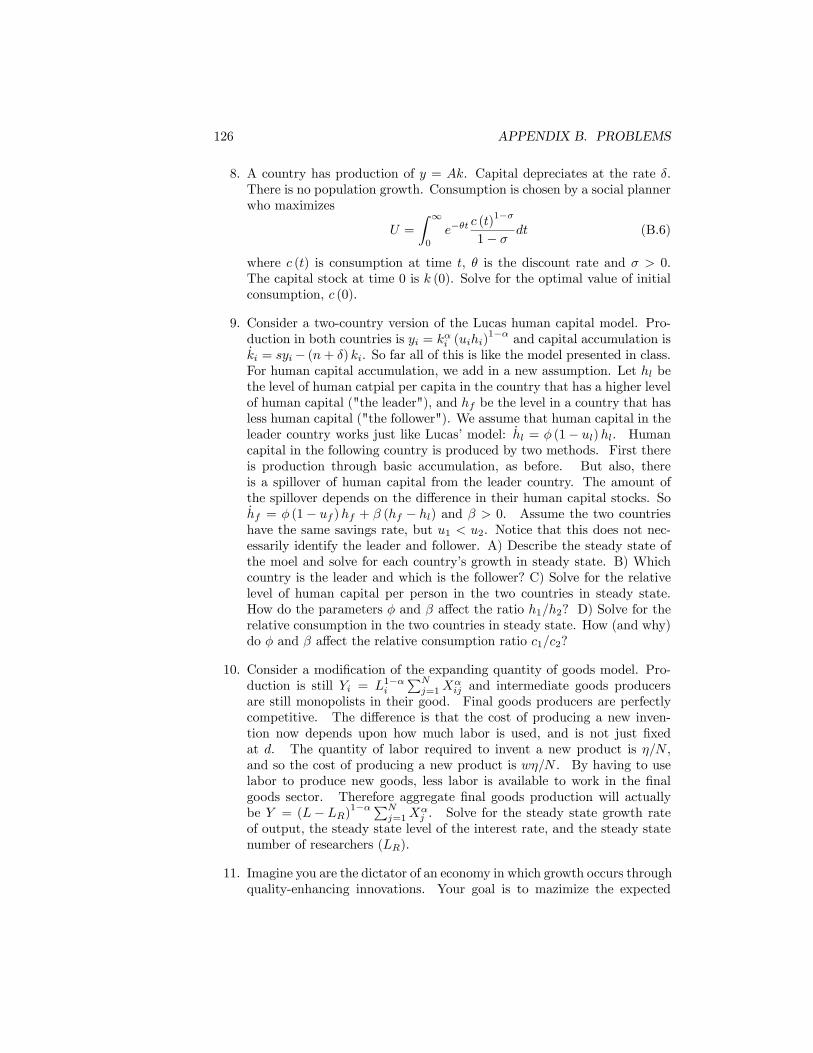
126 APPENDIX B. PROBLEMS
8. A country has production of y = Ak. Capital depreciates at the rate δ.There is no population growth. Consumption is chosen by a social plannerwho maximizes
U =
Z ∞0
e−θtc (t)
1−σ
1− σdt (B.6)
where c (t) is consumption at time t, θ is the discount rate and σ > 0.The capital stock at time 0 is k (0). Solve for the optimal value of initialconsumption, c (0).
9. Consider a two-country version of the Lucas human capital model. Pro-duction in both countries is yi = kαi (uihi)
1−α and capital accumulation iski = syi− (n+ δ) ki. So far all of this is like the model presented in class.For human capital accumulation, we add in a new assumption. Let hl bethe level of human catpial per capita in the country that has a higher levelof human capital ("the leader"), and hf be the level in a country that hasless human capital ("the follower"). We assume that human capital in theleader country works just like Lucas’ model: hl = φ (1− ul)hl. Humancapital in the following country is produced by two methods. First thereis production through basic accumulation, as before. But also, thereis a spillover of human capital from the leader country. The amount ofthe spillover depends on the difference in their human capital stocks. Sohf = φ (1− uf )hf + β (hf − hl) and β > 0. Assume the two countrieshave the same savings rate, but u1 < u2. Notice that this does not nec-essarily identify the leader and follower. A) Describe the steady state ofthe moel and solve for each country’s growth in steady state. B) Whichcountry is the leader and which is the follower? C) Solve for the relativelevel of human capital per person in the two countries in steady state.How do the parameters φ and β affect the ratio h1/h2? D) Solve for therelative consumption in the two countries in steady state. How (and why)do φ and β affect the relative consumption ratio c1/c2?
10. Consider a modification of the expanding quantity of goods model. Pro-duction is still Yi = L1−αi
PNj=1X
αij and intermediate goods producers
are still monopolists in their good. Final goods producers are perfectlycompetitive. The difference is that the cost of producing a new inven-tion now depends upon how much labor is used, and is not just fixedat d. The quantity of labor required to invent a new product is η/N ,and so the cost of producing a new product is wη/N . By having to uselabor to produce new goods, less labor is available to work in the finalgoods sector. Therefore aggregate final goods production will actuallybe Y = (L− LR)
1−αPNj=1X
αj . Solve for the steady state growth rate
of output, the steady state level of the interest rate, and the steady statenumber of researchers (LR).
11. Imagine you are the dictator of an economy in which growth occurs throughquality-enhancing innovations. Your goal is to mazimize the expected
B.5. ENDOGENOUS GROWTH 127
present value of consumption yt or
maxU =
Z ∞0
e−rtE (yt) dt (B.7)
and given the quality model the income in period t is described by
E (yt) =∞Xk=0
Π (k, t)Akxα (B.8)
where Π (k, t) is the probability that exactly k innovations will occur upto time t. With a constant choice of n, and the Poisson process for inno-vations, statistics tell us that
Π (k, t) =(λnt)k
k!e−λnt. (B.9)
A) So you, as the social planner, need to choose x and n to maximize Usubject to the constraint that L = x + n. You’ll need to use the factthat Ak = A0γ
k as well. B) Compare the optimal level of n you foundas a social planner with the optimal n that we found in the decentralizedeconomy - under what conditions on the parameters will growth in thedecentralized economy be too fast?

128 APPENDIX B. PROBLEMS

Bibliography
[1] Aghion, Philippe and Peter Howitt (1992), "A Model of Growth throughCreative Destruction," Econometrica, 60(2), 323-351.
[2] Aiyagari, S. Rao (1994), "Uninsured Idiosyncratic Risk and Aggregate Sav-ing," Quarterly Journal of Economics, 109, 659-684.
[3] Barro, Robert J. (1974), "Are Government Bonds Net Wealth?" Journalof Political Economy, 81(6), 1095-1117.
[4] Barro, Robert J. (1997), Determinants of Economic Growth: A Cross-Country Empirical Study, Cambridge, MA: MIT Press.
[5] Barro, Robert J. and Gary S. Becker (1989), "Fertility Choice in a Modelof Economic Growth," Econometrica, 57, 481-501.
[6] Barro, Robert J. and N. Gregory Mankiw and Xavier Sala-i-Martin (1995),"Capital Mobility in Neoclassical Models of Growth," American EconomicReview, 85, 103-115.
[7] Barro, Robert J. and Xavier Sala-i-Martin (1992), "Convergence," Journalof Political Economy, 100, 223-251.
[8] Barro, Robert J. and Xavier Sala-i-Martin (1995), Economic Growth,McGraw-Hill, New York.
[9] Becker, Gary and Kevin Murphy and Robert Tamura (1990) "Human Cap-ital, Fertility, and Economic Growth," Journal of Political Economy, 98(5).
[10] Blanchard, Olivier and Stanley Fischer (1989), Lectures on Macroeco-nomics, MIT Press.
[11] Brock, William and Leonard Mirman (1972), "Optimal Economic Growthand Uncertainty: The Discounted Case," Journal of Economic Theory, 4(3),479-513.
[12] Carroll, Christopher D. (1997), "Buffer Stock Saving and the Life-Cycle/Permanent Income Hypothesis," Quarterly Journal of Economics,112(1), 1-56.
129
130 BIBLIOGRAPHY
[13] Deaton, Angus (1992), Understanding Consumption, Oxford: Oxford Uni-versity Press.
[14] Diamond, Peter (1965), "National Debt in a Neoclassical Growth Model,"American Economic Review, 55, 1126-1150.
[15] Fisher, Irving (1930), The Theory of Interest, MacMillan, New York.
[16] Galor, Oded and David Weil. (2000) "Population, Technology, and Growth:From Malthusian Stagnation to the Demographic Transition," AmericanEconomic Review, 90(4).
[17] Grossman, Gene M. and Elhanan Helpman (1991), Innovation and Growthin the Global Economy, Cambridge: MIT Press.
[18] Hall, Robert E. (1978), "Stochastic Implications of the Life-Cycle/Permanent Income Hypothesis: Theory and Evidence," Journal ofPolitical Economy, 96, 971-987.
[19] Hall, Robert E. and Charles Jones (1999), "Why Do Some Countries Pro-duce So Much More Output per Worker than Others?" Quarterly Journalof Economics, 114, 83-116.
[20] Jones, Charels (1995), "R&D-Based Models of Economic Growth," Journalof Political Economy, 103, 759-784.
[21] King, Robert G. and Charles Plosser and Sergio T. Rebelo (1988), "Pro-duction, Growth, and Business Cycles, I: The Basic Neoclassical Model andII: New Directions," Journal of Monetary Economics, 21(2/3), 195-232 and309-341.
[22] Kremer, Michael (1993), "Population Growth and Technological Change:One Million B.C. to 1990," Quarterly Journal of Economics, 108(3), 681-716.
[23] Kydland, Finn E. and Edward Prescott (1982), "Time to Build and Aggre-gate Fluctuations," Econometrica, 50(6), 1345-1370.
[24] Lucas, Robert E. (1988), "On the Mechanics of Economic Development,"Journal of Monetary Economics, 22, 3-42.
[25] Mankiw, N. Gregory (1982), "Hall’s Consumption Hypothesis and DurableGoods," Journal of Monetary Economics, 10(3), 417-425.
[26] Mankiw, N. Gregory and David Romer and David Weil (1992), "A Contri-bution to the Empirics of Economic Growth," Quarterly Journal of Eco-nomics, 107(2), 407-437.
[27] Prescott, Edward C. (1986), "Theory Ahead of Business Cycle Measure-ment," Carnegie-Rochester Conference Series on Public Policy, 25, 11-44.
BIBLIOGRAPHY 131
[28] Rebelo, Sergio T. (1991), "Long-Run Policy Analysis and Long-RunGrowth," Journal of Political Economy, 99(3), 500-521.
[29] Romer, Paul M. (1986), "Increasing Returns and Long Run Growth," Jour-nal of Political Economy, 94, 1002-1037.
[30] Romer, Paul M. (1987), "Growth Based on Increasing Returns Due toSpecialization," American Economic Review, 77(2), 56-62.
[31] Romer, Paul M. (1990), "Endogenous Technological Change," Journal ofPolitical Economy, 98(5), S71-S102.
[32] Samuelson, Paul A. (1958), "An Exact Consumption LoanModel of InterestWith or Without the Social Contrivance of Money," Journal of PoliticalEconomy, 66, 467-482.
[33] Solow, Robert M. (1956), "A Contribution to the Theory of EconomicGrowth," Quarterly Journal of Economics, 70(1), 65-94.
[34] Solow, Robert M. (1957), "Technical Change and the Aggregate ProductionFunction," Review of Economics and Statistics, 39, 312-320.
[35] Summers, Lawrence H. (1981), "Capital Taxation and Accumulation in aLife Cycle Growth Model," American Economic Review, 71(4), 533-544.
[36] Uzawa, Hirofumi (1964), "Optimal Growth in a Two-Sector Model of Cap-ital Accumulation," Review of Economic Studies, 31, 1-24.
![The Father Book - Aaron Grad · The Father Book [2011] for guitar and electronics AARON GRAD](https://img.pdfslide.us/doc/110x75/5b86442d7f8b9af12d8c9d46/the-father-book-aaron-the-father-book-2011-for-guitar-and-electronics-aaron.jpg)


![402 - Grad at Grad SLU Presentation[1]Final - Clark](https://img.pdfslide.us/doc/110x75/577cd5441a28ab9e789a53f1/402-grad-at-grad-slu-presentation1final-clark.jpg)