Embed Size (px)
Citation preview
GNSS based Attitude determination with Statisticaland Deterministic Baseline A Priori Information
P. Jurkowski∗,∗∗, P. Henkel∗,∗∗ and C. Gunther∗∗,∗∗∗∗Advanced Navigation Solutions - ANAVS, Gilching, Germany∗∗Technische Universitat Munchen (TUM), Munich, Germany
∗∗∗German Aerospace Center (DLR), Oberpfaffenhofen, Germany
BIOGRAPHIES
Patryk Jurkowski studied electrical engineering andinformation technology at the Technische UniversitatMunchen, Munich, Germany. He completed his bachelorof science in 2010 and received his diploma with a thesison
”Reliable attitude determination with GNSS: Gaussian a
priori knowledge and Kalman filtering“ with distinction in2011. He also received the first prize in Bavaria in the Eu-ropean Satellite Navigation competition in 2010 for a diffe-rential carrier phase positioning system. Patryk worked asa student trainee on EGNOS performance and integrity forGalileo at EADS Astrium from 2006 to 2010. He foundedAdvanced Navigation Solutions - ANAVS in 2011.
Patrick Henkel received his Bachelor, Master and PhDdegrees from the Technische Universitat Munchen, Mu-nich, Germany. In 2010, he graduated with a PhD thesison reliable carrier phase positioning, which received with”summa cum laude“ the highest distinction. Patrick is nowworking towards his habilitation in the field of precise pointpositioning. He visited the Mathematical Geodesy and Po-sitioning group at TU Delft in 2007, and the GPS Lab atStanford University in 2008 and 2010. Patrick received thePierre Contensou Gold Medal at the International Astro-nautical Congress in 2007, the first prize in Bavaria at theEuropean Satellite Navigation Competition in 2010, andthe Vodafone Award for his dissertation in 2011. He is oneof the founders and currently also the managing director ofAdvanced Navigation Solutions - ANAVS.
Christoph Gunther studied theoretical physics at theSwiss Federal Institute of Technology in Zurich. He recei-ved his diploma in 1979 and completed his PhD in 1984.He worked on communication and information theory atBrown Boveri and Ascom Tech. From 1995, he led the de-velopment of mobile phones for GSM and later dual modeGSM/Satellite phones at Ascom. In 1999, he became headof the research department of Ericsson in Nuremberg. Sin-ce 2003, he is the director of the Institute of Communicati-on and Navigation at the German Aerospace Center (DLR)
and since December 2004, he additionally holds a Chair atthe Technische Universitat Munchen (TUM). His researchinterests are in satellite navigation, communication and si-gnal processing.
ABSTRACT
Attitude determination with carrier phase measurementsis becoming increasingly popular for maritime and automo-bile navigation. However, multipath, frequent loss of lock,cycle slips and severe clock drifts prevent reliable integerambiguity resolution especially for low-cost GNSS recei-vers. The reliability of carrier phase ambiguity resolutioncan be improved by a few methods: One option is the useof some baseline a priori information to reduce the integersearch space. This a priori information can be given eitherin a deterministic or stochastic (Jurkowski [1], Jurkowskiet al. [2], Henkel et al. [3]) form. Another option is the useof multi-frequency linear combinations, which increase thewavelength to noise ratio and, thereby, reduce the numberof grid points within the search space volume. A third op-tion is the use of state space models, which exploit the in-ertia of the vehicles and can be efficiently implemented byrecursive least-squares estimation/ Kalman filtering. Final-ly, one can include additional measurements from inertialsensors and/ or further antennas, and perform an on-boardcalibration of double difference measurements.
In this paper, a method is proposed that uses precisecarrier phases for attitude determination without the needof ambiguity resolution: First, a synchronization of dou-ble difference measurements is performed by computinga range correction based on the satellite movement wi-thin the receiver differential clock offset time. Secondly,if the receiver is moving on a straight path, a linear least-squares fitting of a sequence of absolute code-based posi-tion solutions gives an estimate of the path direction and,thus, an on-board calibration of double difference measu-rements can be even performed with the help of the base-line length, pitch and roll angle a priori information and
satellite-receiver direction vectors. The calibrated carrierphases can then be coasted without the need of ambiguityresolution. The observed accuracy is0.5◦/ baseline length,i.e.0.5◦ for a baseline length of 1 m an0.005◦ for a baseli-ne length of100 m.
The proposed algorithm was tested with real measure-ments from two low-cost, single frequency u-blox LEA6T receivers mounted on the roof of a car and comparedwith the high precision INS/GPS coupled navigation sy-stem iTraceRT-F400 of iMAR as a reference sensor. Themeasurement results show that our kinematic calibration ofthe double difference phases provides a heading accuracythat is sufficient for most applications.
Secondly, a Maximum Likelihood (ML) and MaximumA posteriori Probability (MAP) estimation of ambiguitiesand baselines is proposed. These estimators find the op-timum trade-off between an estimator that minimizes on-ly the range residuals (e.g. unconstrained LAMBDA) andone, which minimizes only the distance to the a priori in-formation. The Gaussian a priori knowledge of the baselinelength, pitch, roll and yaw angles serves as a soft constraint,i.e. it gives a certain preference direction but allows someuncertainties in the a priori knowledge. Consequently, theMAP estimation of ambiguities and baselines is faster thanthe unconstrained LAMBDA and also more robust than theconstrained LAMBDA, which uses a deterministic a prioriinformation. The Gaussian a priori information is fully in-tegrated into the float solution, into the integer search (byinequality constraints), and into the fixed baseline solution.
INTRODUCTION
Attitude determination based on GNSS is an intere-sting alternative/ supplement to inertial navigation systems(INS). Inertial navigation sensors enable an accurate po-sitioning during short GPS outages but suffer from drifts,biases and colored noise, which are difficult to model pro-perly. As GNSS provides a drift-free position estimate, it iscommonly used to calibrate INS.
This paper focuses on attitude determination solely ba-sed on GNSS measurements from single frequency lowcost receivers and antennas: Two LEA-6T receivers we-re used, which include temperature compensated crystaloscillators (TCXO) and correspond to the newest GPS-receiver series (with raw data output) of u-blox. The anten-nas were low-cost patch antennas with10 MHz bandwidthand an integrated low noise amplifier with27 dB gain. The-se receivers suffer from frequent phase jumps due to unre-liable tracking, severe code multipath, substantial antennaphase center variations, and clock oscillations that are toolarge to be canceled by double differencing.
For automobile applications, the baseline length is justaround1 m, which makes the use of carrier phase measu-rements indispensable for attitude determination. However,carrier phase measurements are ambiguous, and the deve-
lopment of methods for their reliable resolution has recei-ved a lot of attraction during the last years. Approachesinclude the coupling of GNSS and INS measurements, theuse of multi-frequency linear combinations to increase theambiguity discrimination [4, 5, 6], the introduction of apriori knowledge [7, 2], and the use of multi-antenna sy-stems. Ambiguity resolution uses the code and carrier pha-se measurements as provided by the delay locked loop andphase locked loop. Note that the integer search is not dis-cussed in this paper as it is described in detail in [8, 9, 10].
CALIBRATION OF DOUBLE DIFFERENCE CAR-RIER PHASE MEASUREMENTS
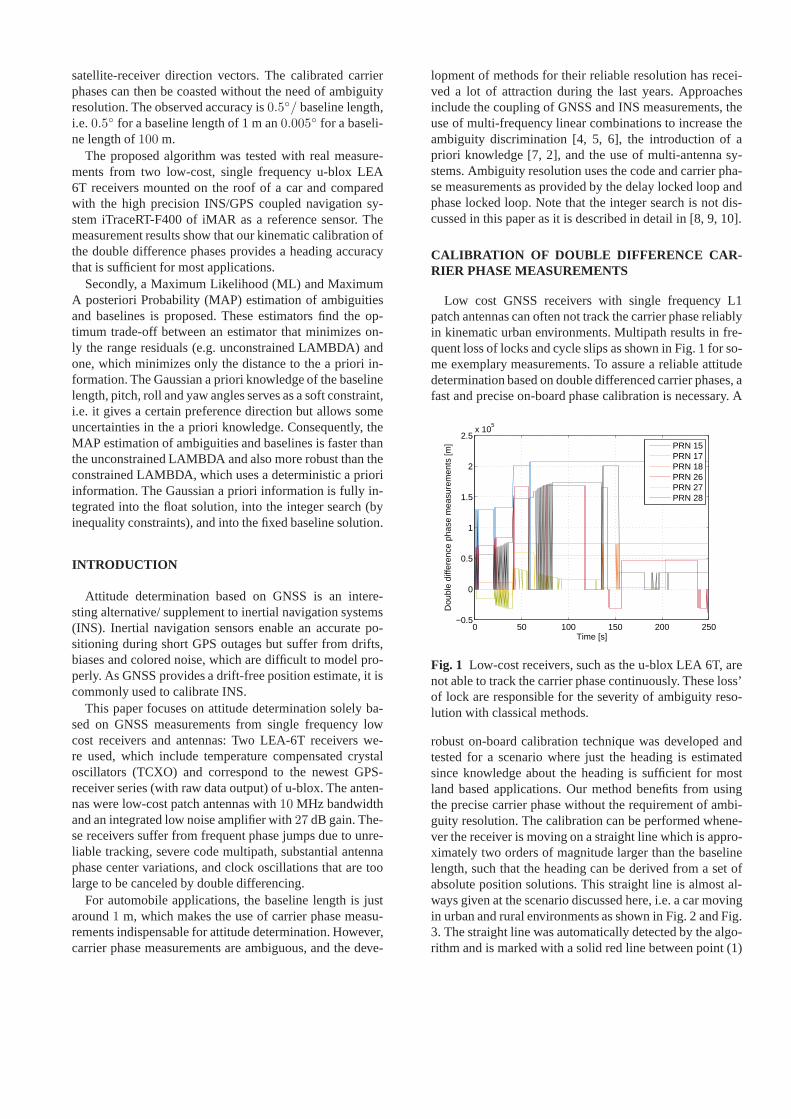
Low cost GNSS receivers with single frequency L1patch antennas can often not track the carrier phase reliablyin kinematic urban environments. Multipath results in fre-quent loss of locks and cycle slips as shown in Fig. 1 for so-me exemplary measurements. To assure a reliable attitudedetermination based on double differenced carrier phases,afast and precise on-board phase calibration is necessary. A
0 50 100 150 200 250−0.5
0
0.5
1
1.5
2
2.5x 10
5
Time [s]
Dou
ble
diffe
renc
e ph
ase
mea
sure
men
ts [m
]
PRN 15PRN 17PRN 18PRN 26PRN 27PRN 28
Fig. 1 Low-cost receivers, such as the u-blox LEA 6T, arenot able to track the carrier phase continuously. These loss’of lock are responsible for the severity of ambiguity reso-lution with classical methods.
robust on-board calibration technique was developed andtested for a scenario where just the heading is estimatedsince knowledge about the heading is sufficient for mostland based applications. Our method benefits from usingthe precise carrier phase without the requirement of ambi-guity resolution. The calibration can be performed whene-ver the receiver is moving on a straight line which is appro-ximately two orders of magnitude larger than the baselinelength, such that the heading can be derived from a set ofabsolute position solutions. This straight line is almost al-ways given at the scenario discussed here, i.e. a car movingin urban and rural environments as shown in Fig. 2 and Fig.3. The straight line was automatically detected by the algo-rithm and is marked with a solid red line between point (1)
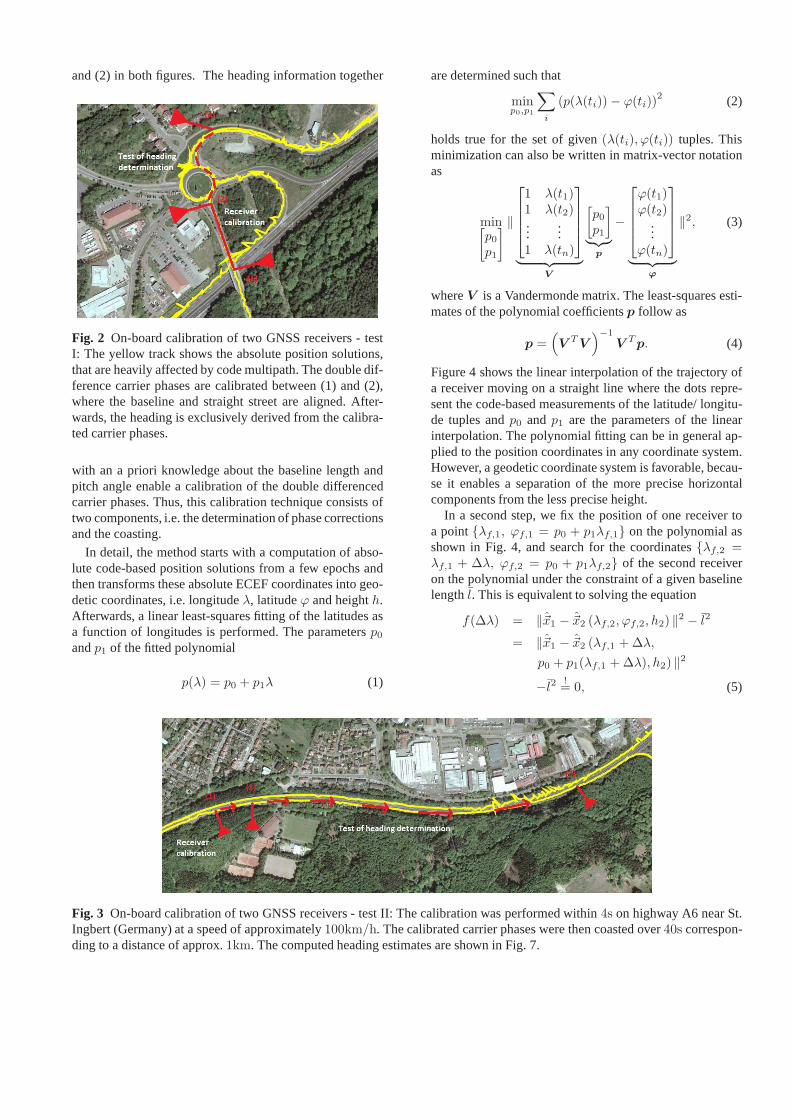
and (2) in both figures. The heading information together
Fig. 2 On-board calibration of two GNSS receivers - testI: The yellow track shows the absolute position solutions,that are heavily affected by code multipath. The double dif-ference carrier phases are calibrated between (1) and (2),where the baseline and straight street are aligned. After-wards, the heading is exclusively derived from the calibra-ted carrier phases.
with an a priori knowledge about the baseline length andpitch angle enable a calibration of the double differencedcarrier phases. Thus, this calibration technique consistsoftwo components, i.e. the determination of phase correctionsand the coasting.
In detail, the method starts with a computation of abso-lute code-based position solutions from a few epochs andthen transforms these absolute ECEF coordinates into geo-detic coordinates, i.e. longitudeλ, latitudeϕ and heighth.Afterwards, a linear least-squares fitting of the latitudesasa function of longitudes is performed. The parametersp0andp1 of the fitted polynomial
p(λ) = p0 + p1λ (1)
are determined such that
minp0,p1
∑
i
(p(λ(ti))− ϕ(ti))2 (2)
holds true for the set of given(λ(ti), ϕ(ti)) tuples. Thisminimization can also be written in matrix-vector notationas
min
p0p1
‖
1 λ(t1)1 λ(t2)...
...1 λ(tn)
︸ ︷︷ ︸
V
[p0p1
]
︸︷︷︸
p
−
ϕ(t1)ϕ(t2)
...ϕ(tn)
︸ ︷︷ ︸
ϕ
‖2, (3)
whereV is a Vandermonde matrix. The least-squares esti-mates of the polynomial coefficientsp follow as
p =(
V TV)−1
V Tp. (4)
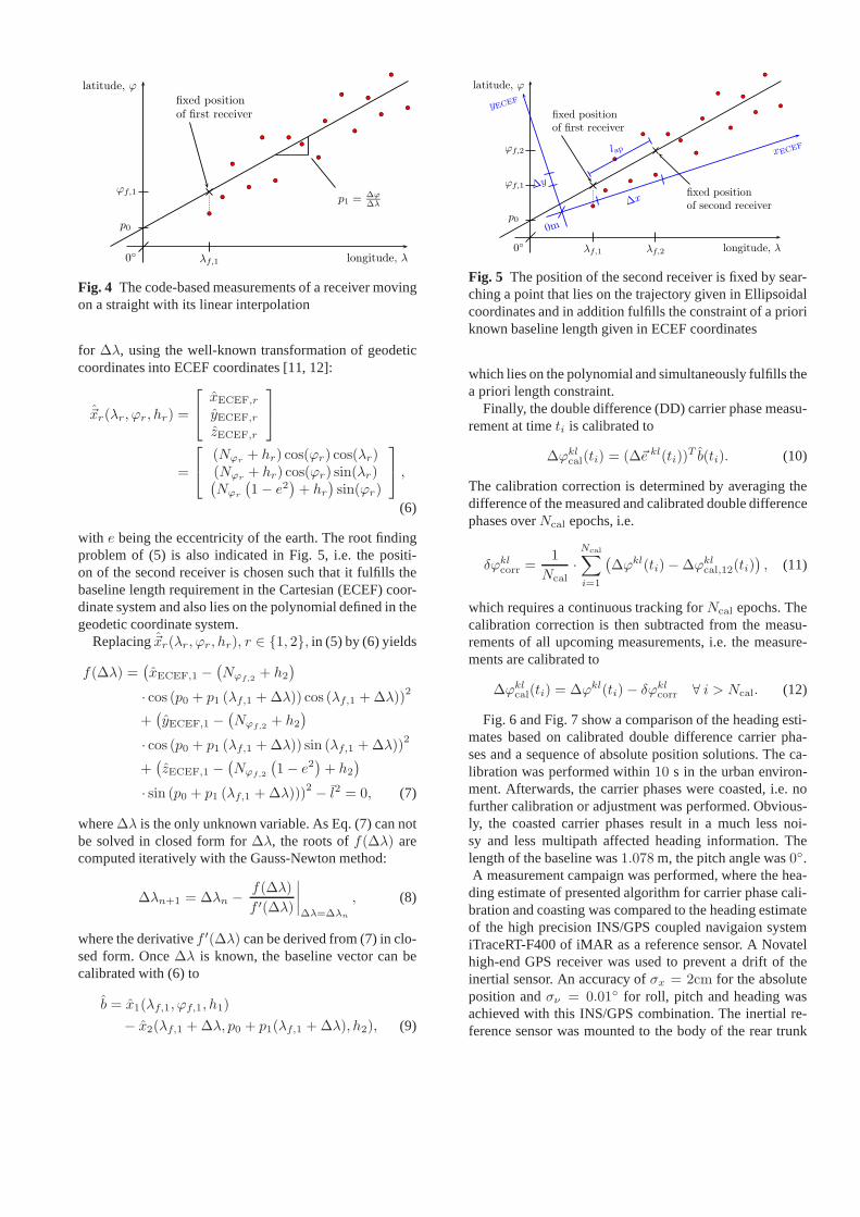
Figure 4 shows the linear interpolation of the trajectory ofa receiver moving on a straight line where the dots repre-sent the code-based measurements of the latitude/ longitu-de tuples andp0 and p1 are the parameters of the linearinterpolation. The polynomial fitting can be in general ap-plied to the position coordinates in any coordinate system.However, a geodetic coordinate system is favorable, becau-se it enables a separation of the more precise horizontalcomponents from the less precise height.
In a second step, we fix the position of one receiver toa point{λf,1, ϕf,1 = p0 + p1λf,1} on the polynomial asshown in Fig. 4, and search for the coordinates{λf,2 =λf,1 + ∆λ, ϕf,2 = p0 + p1λf,2} of the second receiveron the polynomial under the constraint of a given baselinelengthl. This is equivalent to solving the equation
f(∆λ) = ‖~x1 − ~x2 (λf,2, ϕf,2, h2) ‖2 − l2
= ‖~x1 − ~x2 (λf,1 +∆λ,
p0 + p1(λf,1 +∆λ), h2) ‖2
−l2!= 0, (5)
Fig. 3 On-board calibration of two GNSS receivers - test II: The calibration was performed within4s on highway A6 near St.Ingbert (Germany) at a speed of approximately100km/h. The calibrated carrier phases were then coasted over40s correspon-ding to a distance of approx.1km. The computed heading estimates are shown in Fig. 7.
0◦
p0
p1 = ∆ϕ∆λ
λf,1
ϕf,1
fixed position
of first receiver
longitude, λ
latitude, ϕ
bC
bC
bC
bC
bC
bC
bCbC
bC
bC
bC
bC
bC
bC
bC
bC
Fig. 4 The code-based measurements of a receiver movingon a straight with its linear interpolation
for ∆λ, using the well-known transformation of geodeticcoordinates into ECEF coordinates [11, 12]:
~xr(λr, ϕr, hr) =
xECEF,r
yECEF,r
zECEF,r
=
(Nϕr+ hr) cos(ϕr) cos(λr)
(Nϕr+ hr) cos(ϕr) sin(λr)(
Nϕr
(1− e2
)+ hr
)sin(ϕr)
,
(6)
with e being the eccentricity of the earth. The root findingproblem of (5) is also indicated in Fig. 5, i.e. the positi-on of the second receiver is chosen such that it fulfills thebaseline length requirement in the Cartesian (ECEF) coor-dinate system and also lies on the polynomial defined in thegeodetic coordinate system.
Replacing~xr(λr, ϕr, hr), r ∈ {1, 2}, in (5) by (6) yields
f(∆λ) =(xECEF,1 −
(Nϕf,2
+ h2
)
· cos (p0 + p1 (λf,1 +∆λ)) cos (λf,1 +∆λ))2
+(yECEF,1 −
(Nϕf,2
+ h2
)
· cos (p0 + p1 (λf,1 +∆λ)) sin (λf,1 +∆λ))2
+(zECEF,1 −
(Nϕf,2
(1− e2
)+ h2
)
· sin (p0 + p1 (λf,1 +∆λ)))2− l2 = 0, (7)
where∆λ is the only unknown variable. As Eq. (7) can notbe solved in closed form for∆λ, the roots off(∆λ) arecomputed iteratively with the Gauss-Newton method:
∆λn+1 = ∆λn −f(∆λ)
f ′(∆λ)
∣∣∣∣∆λ=∆λn
, (8)
where the derivativef ′(∆λ) can be derived from (7) in clo-sed form. Once∆λ is known, the baseline vector can becalibrated with (6) to
b = x1(λf,1, ϕf,1, h1)
− x2(λf,1 +∆λ, p0 + p1(λf,1 +∆λ), h2), (9)
0◦
p0
λf,1
ϕf,1
λf,2
ϕf,2
fixed position
of first receiver
fixed position
of second receiver
longitude, λ
latitude, ϕ
bC
bC
bC
bC
bC
bC
bCbC
bC
bC
bC
bC
bC
bC
bC
bC
0m
∆x
∆y
xECEF
yECEF
lap
Fig. 5 The position of the second receiver is fixed by sear-ching a point that lies on the trajectory given in Ellipsoidalcoordinates and in addition fulfills the constraint of a prioriknown baseline length given in ECEF coordinates
which lies on the polynomial and simultaneously fulfills thea priori length constraint.
Finally, the double difference (DD) carrier phase measu-rement at timeti is calibrated to
∆ϕklcal(ti) = (∆~e kl(ti))
T b(ti). (10)
The calibration correction is determined by averaging thedifference of the measured and calibrated double differencephases overNcal epochs, i.e.
δϕklcorr =
1
Ncal·
Ncal∑
i=1
(∆ϕkl(ti)−∆ϕkl
cal,12(ti)), (11)
which requires a continuous tracking forNcal epochs. Thecalibration correction is then subtracted from the measu-rements of all upcoming measurements, i.e. the measure-ments are calibrated to
∆ϕklcal(ti) = ∆ϕkl(ti)− δϕkl
corr ∀ i > Ncal. (12)
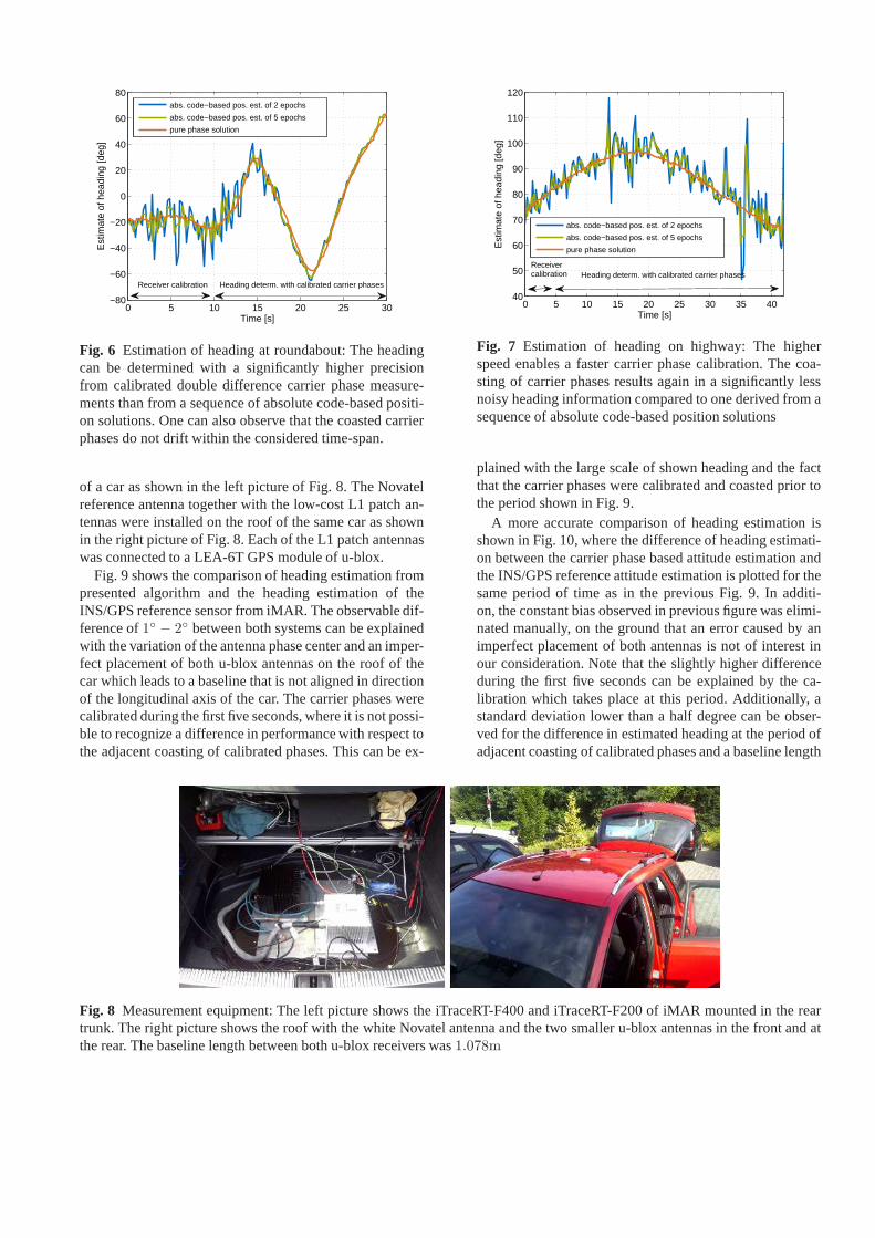
Fig. 6 and Fig. 7 show a comparison of the heading esti-mates based on calibrated double difference carrier pha-ses and a sequence of absolute position solutions. The ca-libration was performed within10 s in the urban environ-ment. Afterwards, the carrier phases were coasted, i.e. nofurther calibration or adjustment was performed. Obvious-ly, the coasted carrier phases result in a much less noi-sy and less multipath affected heading information. Thelength of the baseline was1.078 m, the pitch angle was0◦.A measurement campaign was performed, where the hea-ding estimate of presented algorithm for carrier phase cali-bration and coasting was compared to the heading estimateof the high precision INS/GPS coupled navigaion systemiTraceRT-F400 of iMAR as a reference sensor. A Novatelhigh-end GPS receiver was used to prevent a drift of theinertial sensor. An accuracy ofσx = 2cm for the absoluteposition andσν = 0.01◦ for roll, pitch and heading wasachieved with this INS/GPS combination. The inertial re-ference sensor was mounted to the body of the rear trunk
0 5 10 15 20 25 30−80
−60
−40
−20
0
20
40
60
80
Time [s]
Est
imat
e of
hea
ding
[deg
]
abs. code−based pos. est. of 2 epochs
abs. code−based pos. est. of 5 epochs
pure phase solution
Heading determ. with calibrated carrier phasesReceiver calibration
Fig. 6 Estimation of heading at roundabout: The headingcan be determined with a significantly higher precisionfrom calibrated double difference carrier phase measure-ments than from a sequence of absolute code-based positi-on solutions. One can also observe that the coasted carrierphases do not drift within the considered time-span.
of a car as shown in the left picture of Fig. 8. The Novatelreference antenna together with the low-cost L1 patch an-tennas were installed on the roof of the same car as shownin the right picture of Fig. 8. Each of the L1 patch antennaswas connected to a LEA-6T GPS module of u-blox.
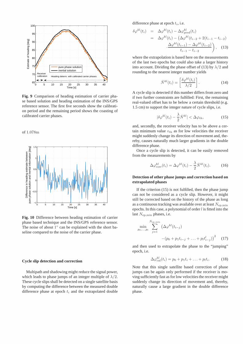
Fig. 9 shows the comparison of heading estimation frompresented algorithm and the heading estimation of theINS/GPS reference sensor from iMAR. The observable dif-ference of1◦ − 2◦ between both systems can be explainedwith the variation of the antenna phase center and an imper-fect placement of both u-blox antennas on the roof of thecar which leads to a baseline that is not aligned in directionof the longitudinal axis of the car. The carrier phases werecalibrated during the first five seconds, where it is not possi-ble to recognize a difference in performance with respect tothe adjacent coasting of calibrated phases. This can be ex-
0 5 10 15 20 25 30 35 4040
50
60
70
80
90
100
110
120
Time [s]
Est
imat
e of
hea
ding
[deg
]
abs. code−based pos. est. of 2 epochs
abs. code−based pos. est. of 5 epochs
pure phase solution
Heading determ. with calibrated carrier phasesReceivercalibration
Fig. 7 Estimation of heading on highway: The higherspeed enables a faster carrier phase calibration. The coa-sting of carrier phases results again in a significantly lessnoisy heading information compared to one derived from asequence of absolute code-based position solutions
plained with the large scale of shown heading and the factthat the carrier phases were calibrated and coasted prior tothe period shown in Fig. 9.
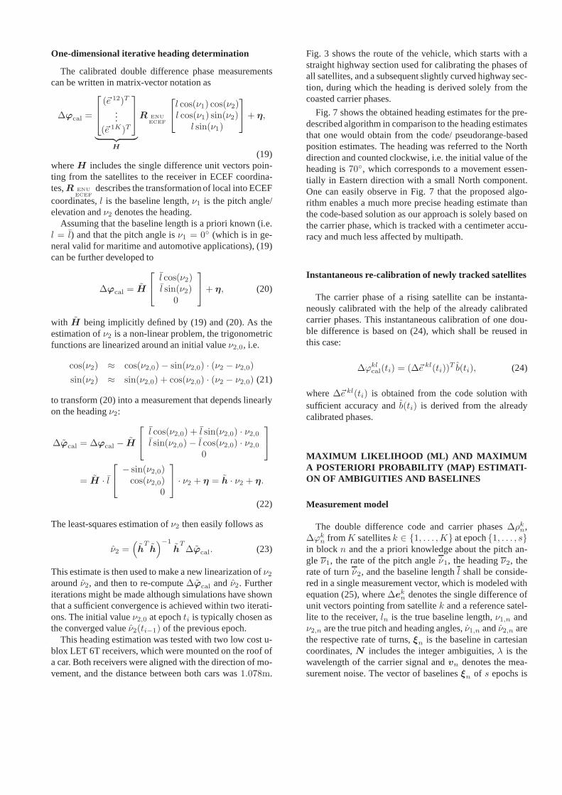
A more accurate comparison of heading estimation isshown in Fig. 10, where the difference of heading estimati-on between the carrier phase based attitude estimation andthe INS/GPS reference attitude estimation is plotted for thesame period of time as in the previous Fig. 9. In additi-on, the constant bias observed in previous figure was elimi-nated manually, on the ground that an error caused by animperfect placement of both antennas is not of interest inour consideration. Note that the slightly higher differenceduring the first five seconds can be explained by the ca-libration which takes place at this period. Additionally, astandard deviation lower than a half degree can be obser-ved for the difference in estimated heading at the period ofadjacent coasting of calibrated phases and a baseline length
Fig. 8 Measurement equipment: The left picture shows the iTraceRT-F400 and iTraceRT-F200 of iMAR mounted in the reartrunk. The right picture shows the roof with the white Novatel antenna and the two smaller u-blox antennas in the front andatthe rear. The baseline length between both u-blox receiverswas1.078m
0 5 10 15 20 25 30 35 4065
70
75
80
85
90
95
100
Time [s]
Est
imat
e of
hea
ding
[deg
]
pure phase solutioninertial solution
Heading determ. with calibrated carrier phasesReceivercalibration
Fig. 9 Comparison of heading estimation of carrier pha-se based solution and heading estimation of the INS/GPSreference sensor. The first five seconds show the calibrati-on period and the remaining period shows the coasting ofcalibrated carrier phases.
of 1.078m
0 5 10 15 20 25 30 35 40−1
−0.5
0
0.5
1
1.5
Diff
eren
ce in
hea
ding
est
imat
e be
twee
npu
re p
hase
sol
utio
n an
d in
ertia
l inf
orm
atio
n [d
eg]
Time [s]
Fig. 10 Difference between heading estimation of carrierphase based technique and the INS/GPS reference sensor.The noise of about1◦ can be explained with the short ba-seline compared to the noise of the carrier phase.
Cycle slip detection and correction
Multipath and shadowing might reduce the signal power,which leads to phase jumps of an integer multiple ofλ/2.These cycle slips shall be detected on a single satellite basisby computing the difference between the measured doubledifference phase at epochti and the extrapolated double
difference phase at epochti, i.e.
δϕkl(ti) = ∆ϕkl(ti)−∆ϕklpred(ti)
= ∆ϕkl(ti)−(∆ϕkl(ti−2 + 2(ti−1 − ti−2)
·∆ϕkl(ti−1)−∆ϕkl(ti−2)
ti−1 − ti−2
)
, (13)
where the extrapolation is based here on the measurementsof the last two epochs but could also take a larger historyinto account. Dividing the phase offset of (13) byλ/2 androunding to the nearest integer number yields
Nkl(ti) =
[δϕkl(ti)
λ/2
]
. (14)
A cycle slip is detected if this number differs from zero andif two further constraints are fulfilled: First, the remainingreal-valued offset has to be below a certain threshold (e.g.1.5 cm) to support the integer nature of cycle slips, i.e.
|δϕkl(ti)−λ
2Nkl| < ∆ϕth, (15)
and, secondly, the receiver velocity has to be above a cer-tain minimum valuevth as for low velocities the receivermight suddenly change its direction of movement and, the-reby, causes naturally much larger gradients in the doubledifference phase.
Once a cycle slip is detected, it can be easily removedfrom the measurements by
∆ϕklcorr(ti) = ∆ϕkl(ti)−
λ
2Nkl(ti). (16)
Detection of other phase jumps and correction based onextrapolated phases
If the criterion (15) is not fulfilled, then the phase jumpcan not be considered as a cycle slip. However, it mightstill be corrected based on the history of the phase as longas a continuous tracking was available over at leastNep,min
epochs. In this case, a polynomial of orderl is fitted into thelastNep,min phases, i.e.
minp0,...,pl
Nep,min∑
j=1
(∆ϕkl(ti−j)
−(p0 + p1ti−j + . . .+ pltli−j)
)2(17)
and then used to extrapolate the phase to the “jumping”epoch, i.e.
∆ϕklcal(ti) = p0 + p1ti + . . .+ plti. (18)
Note that this single satellite based correction of phasejumps can be again only performed if the receiver is mo-ving sufficiently fast as for low velocities the receiver mightsuddenly change its direction of movement and, thereby,naturally cause a large gradient in the double differencephase.
One-dimensional iterative heading determination
The calibrated double difference phase measurementscan be written in matrix-vector notation as
∆ϕcal =
(~e 12)T
...(~e 1K)T
︸ ︷︷ ︸
H
R ENUECEF
l cos(ν1) cos(ν2)l cos(ν1) sin(ν2)
l sin(ν1)
+ η,
(19)whereH includes the single difference unit vectors poin-ting from the satellites to the receiver in ECEF coordina-tes,R ENU
ECEFdescribes the transformation of local into ECEF
coordinates,l is the baseline length,ν1 is the pitch angle/elevation andν2 denotes the heading.
Assuming that the baseline length is a priori known (i.e.l = l) and that the pitch angle isν1 = 0◦ (which is in ge-neral valid for maritime and automotive applications), (19)can be further developed to
∆ϕcal = H
l cos(ν2)l sin(ν2)
0
+ η, (20)
with H being implicitly defined by (19) and (20). As theestimation ofν2 is a non-linear problem, the trigonometricfunctions are linearized around an initial valueν2,0, i.e.
cos(ν2) ≈ cos(ν2,0)− sin(ν2,0) · (ν2 − ν2,0)
sin(ν2) ≈ sin(ν2,0) + cos(ν2,0) · (ν2 − ν2,0) (21)
to transform (20) into a measurement that depends linearlyon the headingν2:
∆ϕcal = ∆ϕcal − H
l cos(ν2,0) + l sin(ν2,0) · ν2,0l sin(ν2,0)− l cos(ν2,0) · ν2,0
0
= H · l
− sin(ν2,0)cos(ν2,0)
0
· ν2 + η = h · ν2 + η.
(22)
The least-squares estimation ofν2 then easily follows as
ν2 =(
hTh)−1
hT∆ϕcal. (23)
This estimate is then used to make a new linearization ofν2aroundν2, and then to re-compute∆ϕcal and ν2. Furtheriterations might be made although simulations have shownthat a sufficient convergence is achieved within two iterati-ons. The initial valueν2,0 at epochti is typically chosen asthe converged valueν2(ti−1) of the previous epoch.
This heading estimation was tested with two low cost u-blox LET 6T receivers, which were mounted on the roof ofa car. Both receivers were aligned with the direction of mo-vement, and the distance between both cars was1.078m.
Fig. 3 shows the route of the vehicle, which starts with astraight highway section used for calibrating the phases ofall satellites, and a subsequent slightly curved highway sec-tion, during which the heading is derived solely from thecoasted carrier phases.
Fig. 7 shows the obtained heading estimates for the pre-described algorithm in comparison to the heading estimatesthat one would obtain from the code/ pseudorange-basedposition estimates. The heading was referred to the Northdirection and counted clockwise, i.e. the initial value of theheading is70◦, which corresponds to a movement essen-tially in Eastern direction with a small North component.One can easily observe in Fig. 7 that the proposed algo-rithm enables a much more precise heading estimate thanthe code-based solution as our approach is solely based onthe carrier phase, which is tracked with a centimeter accu-racy and much less affected by multipath.
Instantaneous re-calibration of newly tracked satellites
The carrier phase of a rising satellite can be instanta-neously calibrated with the help of the already calibratedcarrier phases. This instantaneous calibration of one dou-ble difference is based on (24), which shall be reused inthis case:
∆ϕklcal(ti) = (∆~e kl(ti))
T b(ti), (24)
where∆~e kl(ti) is obtained from the code solution withsufficient accuracy andb(ti) is derived from the alreadycalibrated phases.
MAXIMUM LIKELIHOOD (ML) AND MAXIMUMA POSTERIORI PROBABILITY (MAP) ESTIMATI-ON OF AMBIGUITIES AND BASELINES
Measurement model
The double difference code and carrier phases∆ρkn,∆ϕk
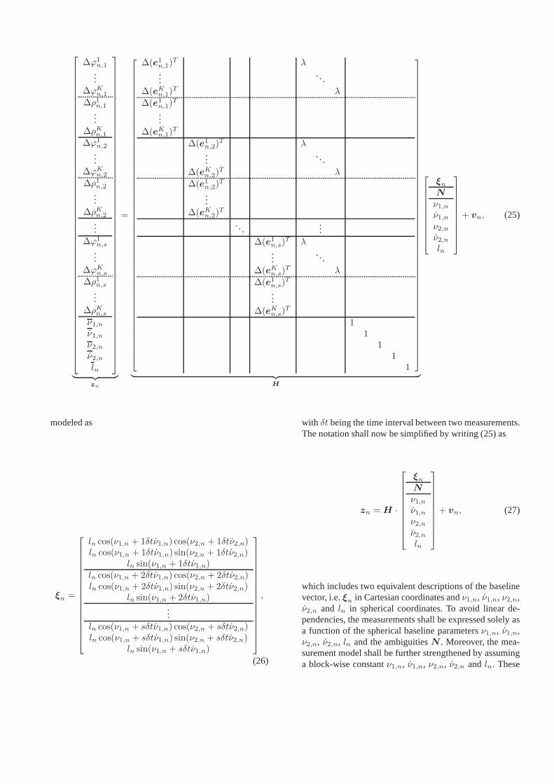
n fromK satellitesk ∈ {1, . . . ,K} at epoch{1, . . . , s}in block n and the a priori knowledge about the pitch an-gle ν1, the rate of the pitch angleν1, the headingν2, therate of turnν2, and the baseline lengthl shall be conside-red in a single measurement vector, which is modeled withequation (25), where∆ekn denotes the single difference ofunit vectors pointing from satellitek and a reference satel-lite to the receiver,ln is the true baseline length,ν1,n andν2,n are the true pitch and heading angles,ν1,n andν2,n arethe respective rate of turns,ξn is the baseline in cartesiancoordinates,N includes the integer ambiguities,λ is thewavelength of the carrier signal andvn denotes the mea-surement noise. The vector of baselinesξn of s epochs is
∆ϕ1n,1...
∆ϕKn,1
∆ρ1n,1...
∆ρKn,1∆ϕ1
n,2...
∆ϕKn,2
∆ρ1n,2...
∆ρKn,2...
∆ϕ1n,s
...∆ϕK
n,s
∆ρ1n,s...
∆ρKn,sν1,nν1,nν2,nν2,nln
︸ ︷︷ ︸
zn
=
∆(e1n,1)
T λ...
. . .∆(eK
n,1)T λ
∆(e1n,1)
T
...∆(eK
n,1)T
∆(e1n,2)T λ
.... . .
∆(eKn,2)T λ
∆(e1n,2)T
...∆(eKn,2)
T
. . ....
∆(e1n,s)
T λ...
. . .∆(eK
n,s)T λ
∆(e1n,s)
T
...∆(eK
n,s)T
11
11
1
︸ ︷︷ ︸
H
ξnN
ν1,nν1,nν2,nν2,nln
+ vn, (25)
modeled as
ξn =
ln cos(ν1,n + 1δtν1,n) cos(ν2,n + 1δtν2,n)ln cos(ν1,n + 1δtν1,n) sin(ν2,n + 1δtν2,n)
ln sin(ν1,n + 1δtν1,n)ln cos(ν1,n + 2δtν1,n) cos(ν2,n + 2δtν2,n)ln cos(ν1,n + 2δtν1,n) sin(ν2,n + 2δtν2,n)
ln sin(ν1,n + 2δtν1,n)...
ln cos(ν1,n + sδtν1,n) cos(ν2,n + sδtν2,n)ln cos(ν1,n + sδtν1,n) sin(ν2,n + sδtν2,n)
ln sin(ν1,n + sδtν1,n)
,
(26)
with δt being the time interval between two measurements.The notation shall now be simplified by writing (25) as
zn = H ·
ξnN
ν1,nν1,nν2,nν2,nln
+ vn, (27)
which includes two equivalent descriptions of the baselinevector, i.e.ξn in Cartesian coordinates andν1,n, ν1,n, ν2,n,ν2,n and ln in spherical coordinates. To avoid linear de-pendencies, the measurements shall be expressed solely asa function of the spherical baseline parametersν1,n, ν1,n,ν2,n, ν2,n, ln and the ambiguitiesN . Moreover, the mea-surement model shall be further strengthened by assuminga block-wise constantν1,n, ν1,n, ν2,n, ν2,n and ln. These
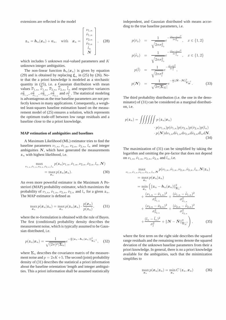
extensions are reflected in the model
zn = hn(xn) + vn, with xn =
ν1,nν1,nν2,nν2,nlnN
, (28)
which includes5 unknown real-valued parameters andKunknown integer ambiguities.
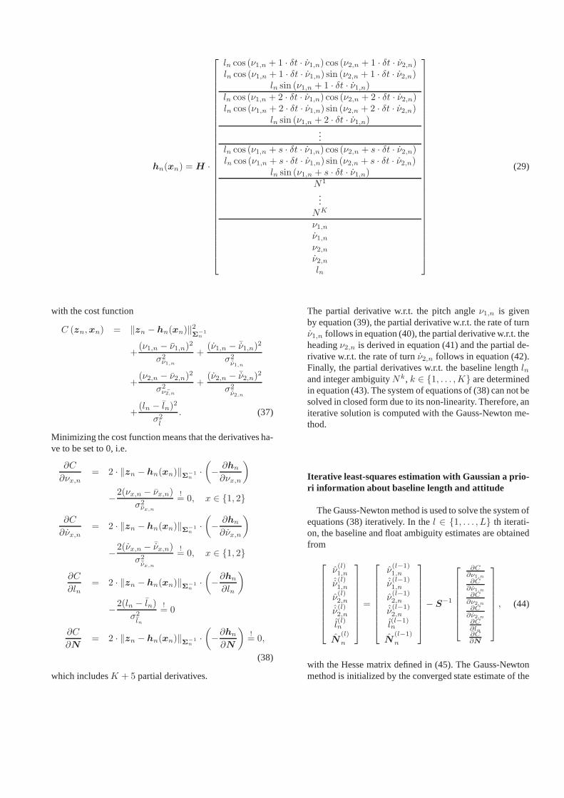
The non-linear functionhn(xn) is given by equation(29) and is obtained by replacingξn in (25) by (26). No-te that the a priori knowledge is modeled as a stochasticquantity in (25), i.e. a Gaussian distribution with meanvaluesν1,n, ν1,n, ν2,n, ν2,n, ln and respective variancesσ2ν1,n
, σ2ν1,n
, σ2ν2,n
, σ2ν2,n
andσ2ln
. The statistical modeling
is advantageous as the true baseline parameters are not per-fectly known in many applications. Consequently, a weigh-ted least-squares baseline estimation based on the measu-rement model of (25) ensures a solution, which representsthe optimum trade-off between low range residuals and abaseline close to the a priori knowledge.
MAP estimation of ambiguities and baselines
A Maximum Likelihood (ML) estimator tries to find thebaseline parametersν1,n, ν1,n, ν2,n, ν2,n, ln and integerambiguitiesN , which have generated the measurementszn with highest likelihood, i.e.
maxν1,n,ν1,n,ν2,n,ν2,n,ln
p(zn|ν1,n, ν1,n, ν2,n, ν2,n, ln,N)
= maxxn
p(zn|xn). (30)
An even more powerful estimator is the Maximum A Po-steriori (MAP) probability estimator, which maximizes theprobability ofν1,n, ν1,n, ν2,n, ν2,n andln for a givenzn.The MAP estimator is defined as
maxxn
p(xn|zn) = maxxn
p(zn|xn) ·p(xn)
p(zn), (31)
where the re-formulation is obtained with the rule of Bayes.The first (conditional) probability density describes themeasurement noise, which is typically assumed to be Gaus-sian distributed, i.e.
p(zn|xn) =1
√
(2π)p|Σn|e− 1
2‖zn−hn(xn)‖2
Σ−1n , (32)
whereΣn describes the covariance matrix of the measure-ment noise andp = 2sK+5. The second (joint) probabilitydensity of (31) describes the statistical a priori informationabout the baseline orientation/ length and integer ambigui-ties. This a priori information shall be assumed statistically
independent, and Gaussian distributed with means accor-ding to the true baseline parameters, i.e.
p(νx) =1
√
2πσ2νx
e−
(νx−νx)2
2σ2νx , x ∈ {1, 2}
p(¯νx) =1
√
2πσ2νx
e− (¯νx−νx)2
2σ2¯νx , x ∈ {1, 2}
p(l) =1
√
2πσ2l
e− (l−l)2
2σ2l ,
p(N) =1
√
2π|ΣN |e− 1
2‖N−N‖2
Σ−1N . (33)
The third probability distribution (i.e. the one in the deno-minator) of (31) can be considered as a marginal distributi-on, i.e.
p(zn) =
∫∫∫∫∫∫
p (zn|xn)
· p(ν1,n)p(ν1,n)p(ν2,n)p(ν2,n)p(ln)
· p(N )dν1,ndν1,ndν2,ndν2,ndlndN .(34)
The maximization of (31) can be simplified by taking thelogarithm and omitting the pre-factor that does not dependonν1,n, ν1,n, ν2,n, ν2,n andln, i.e.
maxν1,n,ν1,n,ν2,n,ν2,n,ln,N
p(ν1,n, ν1,n, ν2,n, ν2,n, ln,N |zn)
= maxxn
p(xn|zn)
= minxn
(
‖zn − hn(xn)‖2Σ
−1n
+(ν1,n − ν1,n)
2
σ2ν1,n
+(ν1,n − ¯ν1,n)
2
σ2¯ν1,n
+(ν2,n − ν2,n)
2
σ2ν2,n
+(ν2,n − ¯ν2,n)
2
σ2¯ν2,n
+(ln − ln)
2
σ2l
+ ‖N − N‖2Σ
−1N
)
, (35)
where the first term on the right side describes the squaredrange residuals and the remaining terms denote the squareddeviation of the unknown baseline parameters from their apriori knowledge. In general, there is no a priori knowledgeavailable for the ambiguities, such that the minimizationsimplifies to
maxxn
p(xn|zn) = minxn
C (zn,xn) (36)
hn(xn) = H ·
ln cos (ν1,n + 1 · δt · ν1,n) cos (ν2,n + 1 · δt · ν2,n)ln cos (ν1,n + 1 · δt · ν1,n) sin (ν2,n + 1 · δt · ν2,n)
ln sin (ν1,n + 1 · δt · ν1,n)ln cos (ν1,n + 2 · δt · ν1,n) cos (ν2,n + 2 · δt · ν2,n)ln cos (ν1,n + 2 · δt · ν1,n) sin (ν2,n + 2 · δt · ν2,n)
ln sin (ν1,n + 2 · δt · ν1,n)...
ln cos (ν1,n + s · δt · ν1,n) cos (ν2,n + s · δt · ν2,n)ln cos (ν1,n + s · δt · ν1,n) sin (ν2,n + s · δt · ν2,n)
ln sin (ν1,n + s · δt · ν1,n)N1
...NK
ν1,nν1,nν2,nν2,nln
(29)
with the cost function
C (zn,xn) = ‖zn − hn(xn)‖2Σ
−1n
+(ν1,n − ν1,n)
2
σ2ν1,n
+(ν1,n − ¯ν1,n)
2
σ2¯ν1,n
+(ν2,n − ν2,n)
2
σ2¯ν2,n
+(ν2,n − ¯ν2,n)
2
σ2¯ν2,n
+(ln − ln)
2
σ2l
. (37)
Minimizing the cost function means that the derivatives ha-ve to be set to 0, i.e.
∂C
∂νx,n= 2 · ‖zn − hn(xn)‖Σ−1
n·
(
−∂hn
∂νx,n
)
−2(νx,n − νx,n)
σ2νx,n
!= 0, x ∈ {1, 2}
∂C
∂νx,n= 2 · ‖zn − hn(xn)‖Σ−1
n·
(
−∂hn
∂νx,n
)
−2(νx,n − ¯νx,n)
σ2¯νx,n
!= 0, x ∈ {1, 2}
∂C
∂ln= 2 · ‖zn − hn(xn)‖Σ−1
n·
(
−∂hn
∂ln
)
−2(ln − ln)
σ2ln
!= 0
∂C
∂N= 2 · ‖zn − hn(xn)‖Σ−1
n·
(
−∂hn
∂N
)
!= 0,
(38)
which includesK + 5 partial derivatives.
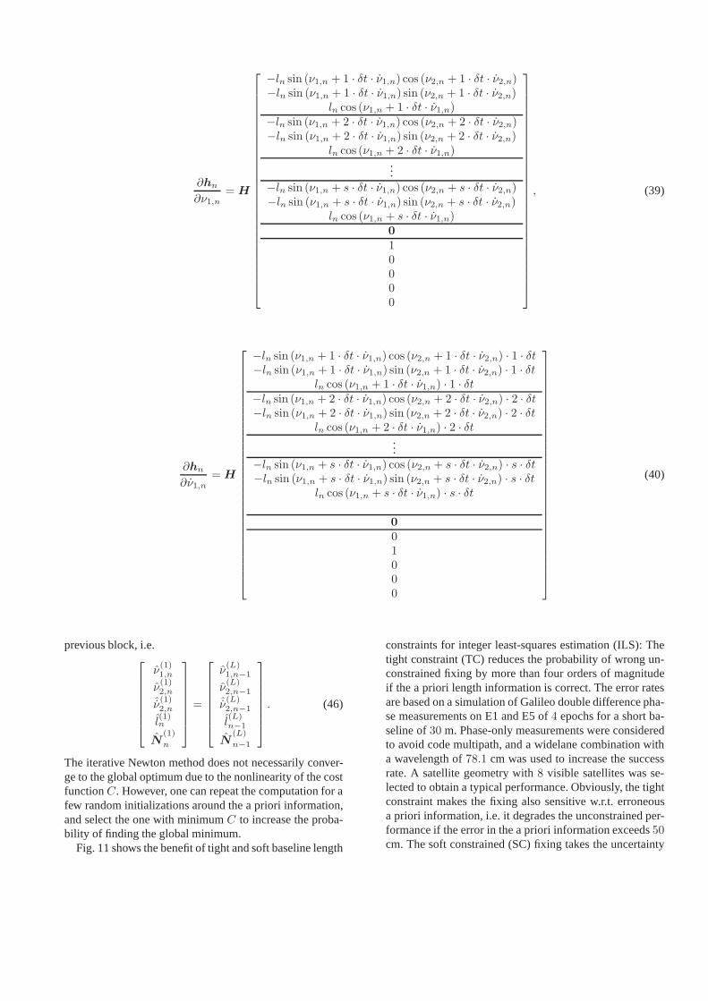
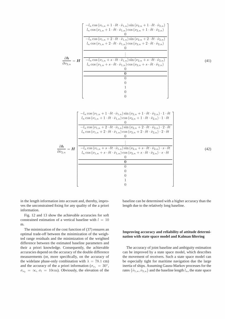
The partial derivative w.r.t. the pitch angleν1,n is givenby equation (39), the partial derivative w.r.t. the rate of turnν1,n follows in equation (40), the partial derivative w.r.t. theheadingν2,n is derived in equation (41) and the partial de-rivative w.r.t. the rate of turnν2,n follows in equation (42).Finally, the partial derivatives w.r.t. the baseline length lnand integer ambiguityNk, k ∈ {1, . . . ,K} are determinedin equation (43). The system of equations of (38) can not besolved in closed form due to its non-linearity. Therefore, aniterative solution is computed with the Gauss-Newton me-thod.
Iterative least-squares estimation with Gaussian a prio-ri information about baseline length and attitude
The Gauss-Newton method is used to solve the system ofequations (38) iteratively. In thel ∈ {1, . . . , L} th iterati-on, the baseline and float ambiguity estimates are obtainedfrom
ν(l)1,n
ˆν(l)1,n
ν(l)2,n
ˆν(l)2,n
l(l)n
N(l)
n
=
ν(l−1)1,n
ˆν(l−1)1,n
ν(l−1)2,n
ˆν(l−1)2,n
l(l−1)n
N(l−1)
n
− S−1
∂C∂ν1,n∂C
∂ν1,n∂C
∂ν2,n∂C
∂ν2,n∂C∂ln∂C∂N
, (44)
with the Hesse matrix defined in (45). The Gauss-Newtonmethod is initialized by the converged state estimate of the
∂hn
∂ν1,n= H
−ln sin (ν1,n + 1 · δt · ν1,n) cos (ν2,n + 1 · δt · ν2,n)−ln sin (ν1,n + 1 · δt · ν1,n) sin (ν2,n + 1 · δt · ν2,n)
ln cos (ν1,n + 1 · δt · ν1,n)−ln sin (ν1,n + 2 · δt · ν1,n) cos (ν2,n + 2 · δt · ν2,n)−ln sin (ν1,n + 2 · δt · ν1,n) sin (ν2,n + 2 · δt · ν2,n)
ln cos (ν1,n + 2 · δt · ν1,n)...
−ln sin (ν1,n + s · δt · ν1,n) cos (ν2,n + s · δt · ν2,n)−ln sin (ν1,n + s · δt · ν1,n) sin (ν2,n + s · δt · ν2,n)
ln cos (ν1,n + s · δt · ν1,n)0
10000
, (39)
∂hn
∂ν1,n= H
−ln sin (ν1,n + 1 · δt · ν1,n) cos (ν2,n + 1 · δt · ν2,n) · 1 · δt−ln sin (ν1,n + 1 · δt · ν1,n) sin (ν2,n + 1 · δt · ν2,n) · 1 · δt
ln cos (ν1,n + 1 · δt · ν1,n) · 1 · δt−ln sin (ν1,n + 2 · δt · ν1,n) cos (ν2,n + 2 · δt · ν2,n) · 2 · δt−ln sin (ν1,n + 2 · δt · ν1,n) sin (ν2,n + 2 · δt · ν2,n) · 2 · δt
ln cos (ν1,n + 2 · δt · ν1,n) · 2 · δt...
−ln sin (ν1,n + s · δt · ν1,n) cos (ν2,n + s · δt · ν2,n) · s · δt−ln sin (ν1,n + s · δt · ν1,n) sin (ν2,n + s · δt · ν2,n) · s · δt
ln cos (ν1,n + s · δt · ν1,n) · s · δt
0
01000
(40)
previous block, i.e.
ν(1)1,n
ν(1)2,n
ˆν(1)2,n
l(1)n
N(1)
n
=
ν(L)1,n−1
ν(L)2,n−1
ˆν(L)2,n−1
l(L)n−1
N(L)
n−1
. (46)
The iterative Newton method does not necessarily conver-ge to the global optimum due to the nonlinearity of the costfunctionC. However, one can repeat the computation for afew random initializations around the a priori information,and select the one with minimumC to increase the proba-bility of finding the global minimum.
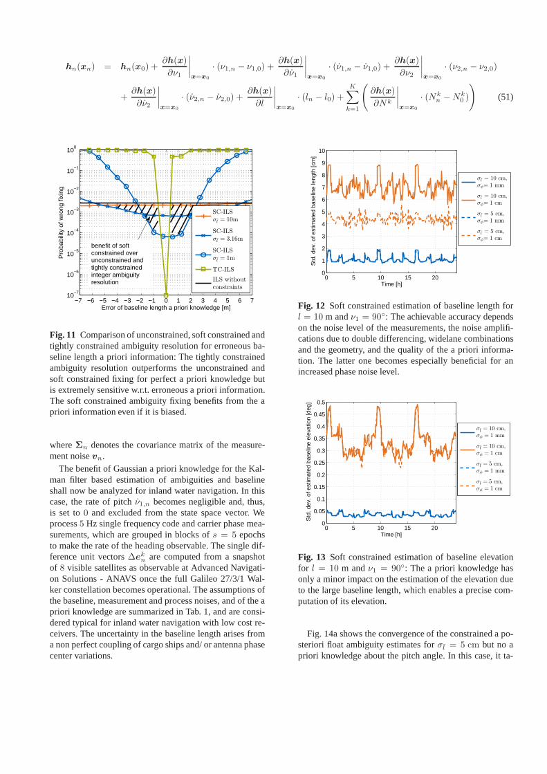
Fig. 11 shows the benefit of tight and soft baseline length
constraints for integer least-squares estimation (ILS): Thetight constraint (TC) reduces the probability of wrong un-constrained fixing by more than four orders of magnitudeif the a priori length information is correct. The error ratesare based on a simulation of Galileo double difference pha-se measurements on E1 and E5 of4 epochs for a short ba-seline of30 m. Phase-only measurements were consideredto avoid code multipath, and a widelane combination witha wavelength of78.1 cm was used to increase the successrate. A satellite geometry with8 visible satellites was se-lected to obtain a typical performance. Obviously, the tightconstraint makes the fixing also sensitive w.r.t. erroneousa priori information, i.e. it degrades the unconstrained per-formance if the error in the a priori information exceeds50cm. The soft constrained (SC) fixing takes the uncertainty
∂h
∂ν2,n= H
−ln cos (ν1,n + 1 · δt · ν1,n) sin (ν2,n + 1 · δt · ν2,n)ln cos (ν1,n + 1 · δt · ν1,n) cos (ν2,n + 1 · δt · ν2,n)
0−ln cos (ν1,n + 2 · δt · ν1,n) sin (ν2,n + 2 · δt · ν2,n)ln cos (ν1,n + 2 · δt · ν1,n) cos (ν2,n + 2 · δt · ν2,n)
0...
−ln cos (ν1,n + s · δt · ν1,n) sin (ν2,n + s · δt · ν2,n)ln cos (ν1,n + s · δt · ν1,n) cos (ν2,n + s · δt · ν2,n)
00
00100
(41)
∂h
∂ν2,n= H
−ln cos (ν1,n + 1 · δt · ν1,n) sin (ν2,n + 1 · δt · ν2,n) · 1 · δtln cos (ν1,n + 1 · δt · ν1,n) cos (ν2,n + 1 · δt · ν2,n) · 1 · δt
0−ln cos (ν1,n + 2 · δt · ν1,n) sin (ν2,n + 2 · δt · ν2,n) · 2 · δtln cos (ν1,n + 2 · δt · ν1,n) cos (ν2,n + 2 · δt · ν2,n) · 2 · δt
0...
−ln cos (ν1,n + s · δt · ν1,n) sin (ν2,n + s · δt · ν2,n) · s · δtln cos (ν1,n + s · δt · ν1,n) cos (ν2,n + s · δt · ν2,n) · s · δt
00
00010
(42)
in the length information into account and, thereby, impro-ves the unconstrained fixing for any quality of the a prioriinformation.
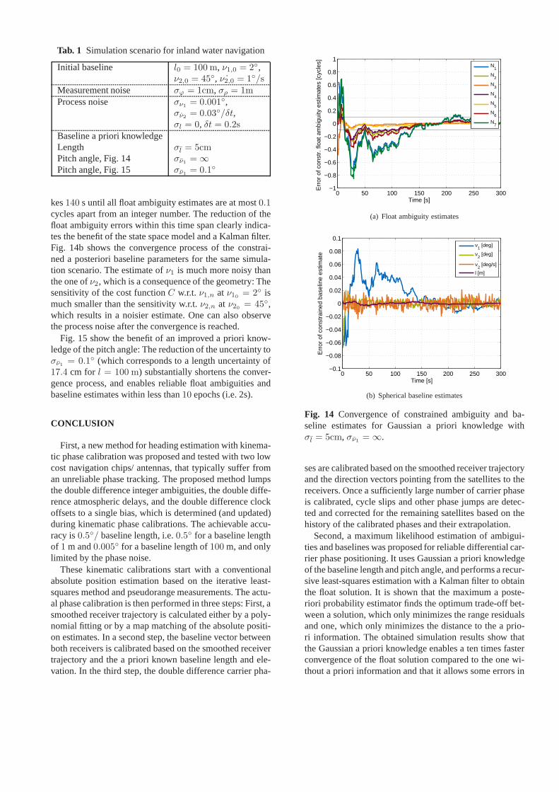
Fig. 12 and 13 show the achievable accuracies for softconstrained estimation of a vertical baseline withl = 10m.
The minimization of the cost function of (37) ensures anoptimal trade-off between the minimization of the weigh-ted range residuals and the minimization of the weighteddifference between the estimated baseline parameters andtheir a priori knowledge. Consequently, the achievableaccuracies depend on the accuracy of the double differencemeasurements (or, more specifically, on the accuracy ofthe widelane phase-only combination withλ = 78.1 cm)and the accuracy of the a priori information (σν1 = 30◦,σν2 = ∞, σl = 10cm). Obviously, the elevation of the
baseline can be determined with a higher accuracy than thelength due to the relatively long baseline.
Improving accuracy and reliability of attitude determi-nation with state space model and Kalman filtering
The accuracy of joint baseline and ambiguity estimationcan be improved by a state space model, which describesthe movement of receivers. Such a state space model canbe especially tight for maritime navigation due the largeinertia of ships. Assuming Gauss-Markov processes for therates{ν1,n, ν2,n} and the baseline lengthln, the state space
∂h
∂ln= H
cos (ν1,n + 1 · δt · ν1,n) cos (ν2,n + 1 · δt · ν2,n)cos (ν1,n + 1 · δt · ν1,n) sin (ν2,n + 1 · δt · ν2,n)
sin (ν1,n + 1 · δt · ν1,n)cos (ν1,n + 2 · δt · ν1,n) cos (ν2,n + 2 · δt · ν2,n)cos (ν1,n + 2 · δt · ν1,n) sin (ν2,n + 2 · δt · ν2,n)
sin (ν1,n + 2 · δt · ν1,n)...
cos (ν1,n + s · δt · ν1,n) cos (ν2,n + s · δt · ν2,n)cos (ν1,n + s · δt · ν1,n) sin (ν2,n + s · δt · ν2,n)
sin (ν1,n + s · δt · ν1,n)0
00001
,∂h
∂Nk= H
000000...000
0k−1×1
10K−k×1
0...0
(43)
S =
∂2C∂2ν1,n
∂2C∂ν1,n∂ν1,n
∂2C∂ν1,n∂ν2,n
∂2C∂ν1,n∂ν2,n
∂2C∂ν1,n∂ln
∂2C∂ν1,n∂N
∂2C∂ν1,n∂ν1,n
∂2C∂2ν1,n
∂2C∂ν1,n∂ν2,n
∂2C∂ν1,n∂ν2,n
∂2C∂ν1,n∂ln
∂2C∂ν1,n∂N
∂2C∂ν2,n∂ν1,n
∂2C∂ν2,nν1,n
∂2C∂2ν2,n
∂2C∂ν2,nν2,n
∂2C∂ν2,nln
∂2C∂ν2,n∂N
∂2C∂ν2,n∂ν1,n
∂2C∂ν2,n∂ν1,n
∂2C∂ν2,n∂ν2,n
∂2C∂2ν2,n
∂2C∂ν2,n∂ln
∂2C∂ν2,n∂N
∂2C∂ln∂ν1,n
∂2C∂ln∂ν1,n
∂2C∂ln∂ν2,n
∂2C∂ln∂ν2,n
∂2C∂2ln
∂2C∂ln∂N
∂2C∂N∂ν1,n
∂2C∂N∂ν1,n
∂2C∂N∂ν2,n
∂2C∂N∂ν2,n
∂2C∂N∂ln
∂2C∂2N
(45)
model is obtained as
ν1,nν1,nν2,nν2,nlnN
︸ ︷︷ ︸
xn
=
1 s · δt1
1 s · δt1
11
︸ ︷︷ ︸
Φ
ν1,n−1
ν1,n−1
ν2,n−1
ν2,n−1
ln−1
N
︸ ︷︷ ︸
xn−1
+
wν1,n
wν1,n
wν2,n
wν2,n
wln
wN
︸ ︷︷ ︸
wn
. (47)
This state space model is included into the MAP estimati-on by a Kalman filter, which combines the GNSS measure-ments, the a priori information and the state space model.The Kalman filter includes a linear prediction of the stateestimate from one block to the next one, i.e.
x−n+1 = Φnx
+n
P x−
n+1= ΦnP x+
nΦ
Tn +Qn+1, (48)
where the second row describes the process noise cova-riance matrix obtained by error propagation. Once the newmeasurement is available, the state estimate is updated, i.e.
x+n = x
−n +Kn
(zn − hn(x
−n )), (49)
whereKn is the Kalman gain, which is computed such thatthe variance of the norm of the a posteriori state estimate isminimized, i.e.
Kn = argminKn
E{‖x+n − E{x+
n }‖2}. (50)
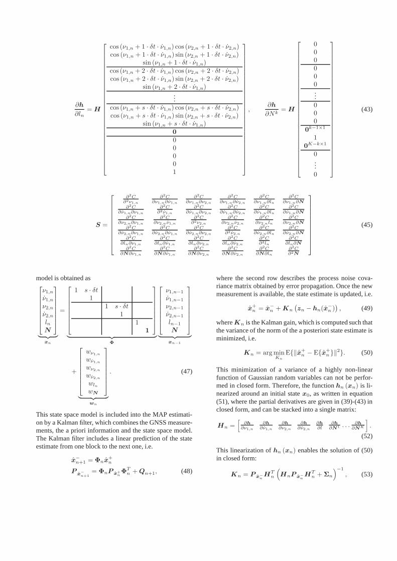
This minimization of a variance of a highly non-linearfunction of Gaussian random variables can not be perfor-med in closed form. Therefore, the functionhn (xn) is li-nearized around an initial statex0, as written in equation(51), where the partial derivatives are given in (39)-(43) inclosed form, and can be stacked into a single matrix:
Hn =[
∂h∂ν1,n
∂h∂ν1,n
∂h∂ν2,n
∂h∂ν2,n
∂h∂l
∂h∂N1 . . .
∂h∂NK
]
.
(52)
This linearization ofhn (xn) enables the solution of (50)in closed form:
Kn = P x−
nHT
n
(
HnP x−
nHT
n +Σn
)−1
, (53)
hn(xn) = hn(x0) +∂h(x)
∂ν1
∣∣∣∣x=x0
· (ν1,n − ν1,0) +∂h(x)
∂ν1
∣∣∣∣x=x0
· (ν1,n − ν1,0) +∂h(x)
∂ν2
∣∣∣∣x=x0
· (ν2,n − ν2,0)
+∂h(x)
∂ν2
∣∣∣∣x=x0
· (ν2,n − ν2,0) +∂h(x)
∂l
∣∣∣∣x=x0
· (ln − l0) +
K∑
k=1
(
∂h(x)
∂Nk
∣∣∣∣x=x0
· (Nkn −Nk
0 )
)
(51)
−7 −6 −5 −4 −3 −2 −1 0 1 2 3 4 5 6 710
−7
10−6
10−5
10−4
10−3
10−2
10−1
100
Error of baseline length a priori knowledge [m]
Pro
babi
lity
of w
rong
fixi
ng
SC-ILS
σl = 10m
SC-ILS
σl = 3.16m
SC-ILS
σl = 1m
TC-ILS
ILS without
constraints
benefit of softconstrained overunconstrained andtightly constrainedinteger ambiguityresolution
Fig. 11 Comparison of unconstrained, soft constrained andtightly constrained ambiguity resolution for erroneous ba-seline length a priori information: The tightly constrainedambiguity resolution outperforms the unconstrained andsoft constrained fixing for perfect a priori knowledge butis extremely sensitive w.r.t. erroneous a priori information.The soft constrained ambiguity fixing benefits from the apriori information even if it is biased.
whereΣn denotes the covariance matrix of the measure-ment noisevn.
The benefit of Gaussian a priori knowledge for the Kal-man filter based estimation of ambiguities and baselineshall now be analyzed for inland water navigation. In thiscase, the rate of pitchν1,n becomes negligible and, thus,is set to0 and excluded from the state space vector. Weprocess5 Hz single frequency code and carrier phase mea-surements, which are grouped in blocks ofs = 5 epochsto make the rate of the heading observable. The single dif-ference unit vectors∆ek
n are computed from a snapshotof 8 visible satellites as observable at Advanced Navigati-on Solutions - ANAVS once the full Galileo 27/3/1 Wal-ker constellation becomes operational. The assumptions ofthe baseline, measurement and process noises, and of the apriori knowledge are summarized in Tab. 1, and are consi-dered typical for inland water navigation with low cost re-ceivers. The uncertainty in the baseline length arises froma non perfect coupling of cargo ships and/ or antenna phasecenter variations.
0 5 10 15 200
1
2
3
4
5
6
7
8
9
10
Time [h]
Std
. dev
. of e
stim
ated
bas
elin
e le
ngth
[cm
]
σl = 10 cm,
σφ= 1 mm
σl = 10 cm,
σφ= 1 cm
σl = 5 cm,
σφ= 1 mm
σl = 5 cm,
σφ= 1 cm
Fig. 12 Soft constrained estimation of baseline length forl = 10 m andν1 = 90◦: The achievable accuracy dependson the noise level of the measurements, the noise amplifi-cations due to double differencing, widelane combinationsand the geometry, and the quality of the a priori informa-tion. The latter one becomes especially beneficial for anincreased phase noise level.
0 5 10 15 200
0.05
0.1
0.15
0.2
0.25
0.3
0.35
0.4
0.45
0.5
Time [h]
Std
. dev
. of e
stim
ated
bas
elin
e el
evat
ion
[deg
]
σl = 10 cm,
σφ = 1 mm
σl = 10 cm,
σφ = 1 cm
σl = 5 cm,
σφ = 1 mm
σl = 5 cm,
σφ = 1 cm
Fig. 13 Soft constrained estimation of baseline elevationfor l = 10 m andν1 = 90◦: The a priori knowledge hasonly a minor impact on the estimation of the elevation dueto the large baseline length, which enables a precise com-putation of its elevation.
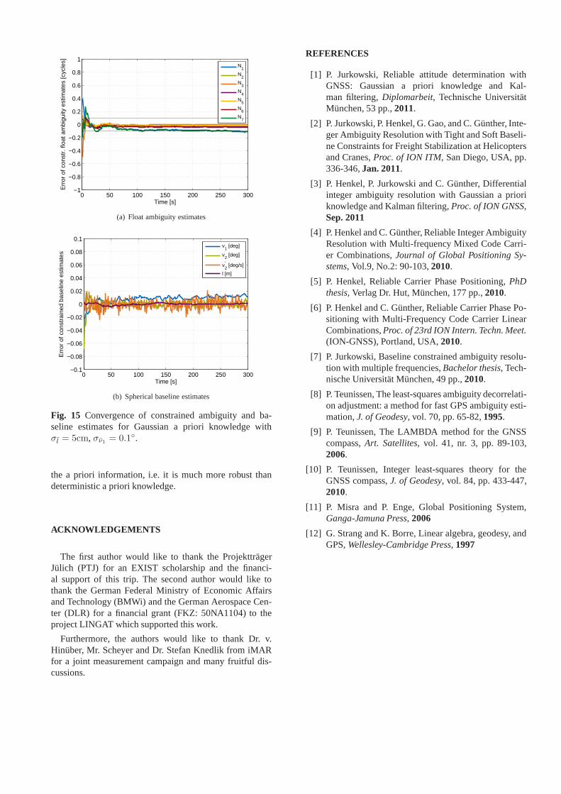
Fig. 14a shows the convergence of the constrained a po-steriori float ambiguity estimates forσl = 5 cm but no apriori knowledge about the pitch angle. In this case, it ta-
Tab. 1 Simulation scenario for inland water navigation
Initial baseline l0 = 100 m, ν1,0 = 2◦,ν2,0 = 45◦, ˙ν2,0 = 1◦/s
Measurement noise σϕ = 1cm, σρ = 1mProcess noise σν1 = 0.001◦,
σν2 = 0.03◦/δt,σl = 0, δt = 0.2s
Baseline a priori knowledgeLength σl = 5cmPitch angle, Fig. 14 σν1 = ∞Pitch angle, Fig. 15 σν1 = 0.1◦
kes140 s until all float ambiguity estimates are at most0.1cycles apart from an integer number. The reduction of thefloat ambiguity errors within this time span clearly indica-tes the benefit of the state space model and a Kalman filter.Fig. 14b shows the convergence process of the constrai-ned a posteriori baseline parameters for the same simula-tion scenario. The estimate ofν1 is much more noisy thanthe one ofν2, which is a consequence of the geometry: Thesensitivity of the cost functionC w.r.t. ν1,n at ν10 = 2◦ ismuch smaller than the sensitivity w.r.t.ν2,n at ν20 = 45◦,which results in a noisier estimate. One can also observethe process noise after the convergence is reached.
Fig. 15 show the benefit of an improved a priori know-ledge of the pitch angle: The reduction of the uncertainty toσν1 = 0.1◦ (which corresponds to a length uncertainty of17.4 cm for l = 100 m) substantially shortens the conver-gence process, and enables reliable float ambiguities andbaseline estimates within less than10 epochs (i.e. 2s).
CONCLUSION
First, a new method for heading estimation with kinema-tic phase calibration was proposed and tested with two lowcost navigation chips/ antennas, that typically suffer froman unreliable phase tracking. The proposed method lumpsthe double difference integer ambiguities, the double diffe-rence atmospheric delays, and the double difference clockoffsets to a single bias, which is determined (and updated)during kinematic phase calibrations. The achievable accu-racy is0.5◦/ baseline length, i.e.0.5◦ for a baseline lengthof 1 m and0.005◦ for a baseline length of100 m, and onlylimited by the phase noise.
These kinematic calibrations start with a conventionalabsolute position estimation based on the iterative least-squares method and pseudorange measurements. The actu-al phase calibration is then performed in three steps: First, asmoothed receiver trajectory is calculated either by a poly-nomial fitting or by a map matching of the absolute positi-on estimates. In a second step, the baseline vector betweenboth receivers is calibrated based on the smoothed receivertrajectory and the a priori known baseline length and ele-vation. In the third step, the double difference carrier pha-
0 50 100 150 200 250 300−1
−0.8
−0.6
−0.4
−0.2
0
0.2
0.4
0.6
0.8
1
Time [s]
Err
or o
f con
str.
floa
t am
bigu
ity e
stim
ates
[cyc
les]
N
1
N2
N3
N4
N5
N6
N7
(a) Float ambiguity estimates
0 50 100 150 200 250 300−0.1
−0.08
−0.06
−0.04
−0.02
0
0.02
0.04
0.06
0.08
0.1
Time [s]
Err
or o
f con
stra
ined
bas
elin
e es
timat
e
ν
1 [deg]
ν2 [deg]
ν′2 [deg/s]
l [m]
(b) Spherical baseline estimates
Fig. 14 Convergence of constrained ambiguity and ba-seline estimates for Gaussian a priori knowledge withσl = 5cm, σν1 = ∞.
ses are calibrated based on the smoothed receiver trajectoryand the direction vectors pointing from the satellites to thereceivers. Once a sufficiently large number of carrier phaseis calibrated, cycle slips and other phase jumps are detec-ted and corrected for the remaining satellites based on thehistory of the calibrated phases and their extrapolation.
Second, a maximum likelihood estimation of ambigui-ties and baselines was proposed for reliable differential car-rier phase positioning. It uses Gaussian a priori knowledgeof the baseline length and pitch angle, and performs a recur-sive least-squares estimation with a Kalman filter to obtainthe float solution. It is shown that the maximum a poste-riori probability estimator finds the optimum trade-off bet-ween a solution, which only minimizes the range residualsand one, which only minimizes the distance to the a prio-ri information. The obtained simulation results show thatthe Gaussian a priori knowledge enables a ten times fasterconvergence of the float solution compared to the one wi-thout a priori information and that it allows some errors in
0 50 100 150 200 250 300−1
−0.8
−0.6
−0.4
−0.2
0
0.2
0.4
0.6
0.8
1
Time [s]
Err
or o
f con
str.
floa
t am
bigu
ity e
stim
ates
[cyc
les]
N
1
N2
N3
N4
N5
N6
N7
(a) Float ambiguity estimates
0 50 100 150 200 250 300−0.1
−0.08
−0.06
−0.04
−0.02
0
0.02
0.04
0.06
0.08
0.1
Time [s]
Err
or o
f con
stra
ined
bas
elin
e es
timat
es
ν
1 [deg]
ν2 [deg]
ν′2 [deg/s]
l [m]
(b) Spherical baseline estimates
Fig. 15 Convergence of constrained ambiguity and ba-seline estimates for Gaussian a priori knowledge withσl = 5cm, σν1 = 0.1◦.
the a priori information, i.e. it is much more robust thandeterministic a priori knowledge.
ACKNOWLEDGEMENTS
The first author would like to thank the ProjekttragerJulich (PTJ) for an EXIST scholarship and the financi-al support of this trip. The second author would like tothank the German Federal Ministry of Economic Affairsand Technology (BMWi) and the German Aerospace Cen-ter (DLR) for a financial grant (FKZ: 50NA1104) to theproject LINGAT which supported this work.
Furthermore, the authors would like to thank Dr. v.Hinuber, Mr. Scheyer and Dr. Stefan Knedlik from iMARfor a joint measurement campaign and many fruitful dis-cussions.
REFERENCES
[1] P. Jurkowski, Reliable attitude determination withGNSS: Gaussian a priori knowledge and Kal-man filtering,Diplomarbeit, Technische UniversitatMunchen, 53 pp.,2011.
[2] P. Jurkowski, P. Henkel, G. Gao, and C. Gunther, Inte-ger Ambiguity Resolution with Tight and Soft Baseli-ne Constraints for Freight Stabilization at Helicoptersand Cranes,Proc. of ION ITM, San Diego, USA, pp.336-346,Jan. 2011.
[3] P. Henkel, P. Jurkowski and C. Gunther, Differentialinteger ambiguity resolution with Gaussian a prioriknowledge and Kalman filtering,Proc. of ION GNSS,Sep. 2011
[4] P. Henkel and C. Gunther, Reliable Integer AmbiguityResolution with Multi-frequency Mixed Code Carri-er Combinations,Journal of Global Positioning Sy-stems, Vol.9, No.2: 90-103,2010.
[5] P. Henkel, Reliable Carrier Phase Positioning,PhDthesis, Verlag Dr. Hut, Munchen, 177 pp.,2010.
[6] P. Henkel and C. Gunther, Reliable Carrier Phase Po-sitioning with Multi-Frequency Code Carrier LinearCombinations,Proc. of 23rd ION Intern. Techn. Meet.(ION-GNSS), Portland, USA,2010.
[7] P. Jurkowski, Baseline constrained ambiguity resolu-tion with multiple frequencies,Bachelor thesis, Tech-nische Universitat Munchen, 49 pp.,2010.
[8] P. Teunissen, The least-squares ambiguity decorrelati-on adjustment: a method for fast GPS ambiguity esti-mation,J. of Geodesy, vol. 70, pp. 65-82,1995.
[9] P. Teunissen, The LAMBDA method for the GNSScompass,Art. Satellites, vol. 41, nr. 3, pp. 89-103,2006.
[10] P. Teunissen, Integer least-squares theory for theGNSS compass,J. of Geodesy, vol. 84, pp. 433-447,2010.
[11] P. Misra and P. Enge, Global Positioning System,Ganga-Jamuna Press, 2006
[12] G. Strang and K. Borre, Linear algebra, geodesy, andGPS,Wellesley-Cambridge Press, 1997