Embed Size (px)
Citation preview
ATTITUDE DETERMINATION SYSTEM FOR NANOSATELLITE USING EXTENDED KALMAN FILTER ON
ARM7TDMI PLATFORM
ADAM AIN BIN MOHD POIN KEUI
UNIVERSITI SAINS MALAYSIA
2014

ATTITUDE DETERMINATION SYSTEM FOR NANO SATELLITE USING
EXTENDED KALMAN FILTER ON ARM7TDMI PLATFORM
by
ADAM AIN BIN MOHD POIN KEUI
Thesis submitted in fulfilment of the requirementsfor the degree of
Master of Science
September 2014

ACKNOWLEDGMENTS
In the name of Allah, the most gracious and the most merciful. First and foremost I
offer my sincerest gratitude to my supervisor, Professor Othman Sidek, who has guided
and supported me with his patience and knowledge throughout my research. I attribute
my accomplishment to his encouragement, patience, effort and without him this thesis
would not have been completed. One simply could not wish for a better and friendlier
supervisor as he is. His suggestions and advices had helped me in my times of despair
when my research were facing some problems.
I also owe my sincerest gratitude to Professor Md Azlin Md Said as my co-supervisor
who also helped me in the completion of my thesis. I would like to extend my gratitude
to Mr Muhammad Fadly Nikmat for also guiding me in my research.
Many thanks to the staffs of Collaborative Microelectronic Design Excellence Cen-
ter (CEDEC) who were involved directly or indirectly in this research work. My ap-
preciation also goes to the School of Electrical and Electronic Engineering (SEEE),
USM for giving me the opportunity to further my studies.
Finally, I would like to thank my parents who has been supporting me with their
patience during the completion of my thesis. I would like to thanks Astronautics Tech-
nology Sdn. Bhd. (ATSB) and Malaysia Space Centre (ANGKASA) for giving me the
opportunity to be involved with the InnoSAT satellite project.
ii
TABLE OF CONTENTS
Acknowledgments . . . . . . . . . . . . . . . . . . . . . . . . . . . . . . . . . . . . . . . . . . . . . . . . . . . . . . . . . . . . . . . . . . . . ii
Table of Contents . . . . . . . . . . . . . . . . . . . . . . . . . . . . . . . . . . . . . . . . . . . . . . . . . . . . . . . . . . . . . . . . . . . . . iii
List of Tables . . . . . . . . . . . . . . . . . . . . . . . . . . . . . . . . . . . . . . . . . . . . . . . . . . . . . . . . . . . . . . . . . . . . . . . . . vi
List of Figures . . . . . . . . . . . . . . . . . . . . . . . . . . . . . . . . . . . . . . . . . . . . . . . . . . . . . . . . . . . . . . . . . . . . . . . . vii
List of Abbreviations . . . . . . . . . . . . . . . . . . . . . . . . . . . . . . . . . . . . . . . . . . . . . . . . . . . . . . . . . . . . . . . . . xi
List of Symbols . . . . . . . . . . . . . . . . . . . . . . . . . . . . . . . . . . . . . . . . . . . . . . . . . . . . . . . . . . . . . . . . . . . . . . . xv
Publication . . . . . . . . . . . . . . . . . . . . . . . . . . . . . . . . . . . . . . . . . . . . . . . . . . . . . . . . . . . . . . . . . . . . . . . . . . . . xviii
Abstrak . . . . . . . . . . . . . . . . . . . . . . . . . . . . . . . . . . . . . . . . . . . . . . . . . . . . . . . . . . . . . . . . . . . . . . . . . . . . . . . . xix
Abstract . . . . . . . . . . . . . . . . . . . . . . . . . . . . . . . . . . . . . . . . . . . . . . . . . . . . . . . . . . . . . . . . . . . . . . . . . . . . . . . xxi
CHAPTER 1 – INTRODUCTION
1.1 Background . . . . . . . . . . . . . . . . . . . . . . . . . . . . . . . . . . . . . . . . . . . . . . . . . . . . . . . . . . . . . . . . . . . . 1
1.2 Problem Statement . . . . . . . . . . . . . . . . . . . . . . . . . . . . . . . . . . . . . . . . . . . . . . . . . . . . . . . . . . . . 2
1.3 Objective of study . . . . . . . . . . . . . . . . . . . . . . . . . . . . . . . . . . . . . . . . . . . . . . . . . . . . . . . . . . . . . 3
1.4 Scope and Limitations . . . . . . . . . . . . . . . . . . . . . . . . . . . . . . . . . . . . . . . . . . . . . . . . . . . . . . . . . 4
1.5 Thesis Organization . . . . . . . . . . . . . . . . . . . . . . . . . . . . . . . . . . . . . . . . . . . . . . . . . . . . . . . . . . . 4
CHAPTER 2 – OVERVIEW OF ATTITUDE DETERMINATION SYSTEMAND ARCHITECTURE
2.1 Introduction . . . . . . . . . . . . . . . . . . . . . . . . . . . . . . . . . . . . . . . . . . . . . . . . . . . . . . . . . . . . . . . . . . . . 5
2.2 Attitude Determination System Architectures . . . . . . . . . . . . . . . . . . . . . . . . . . . . . . . 5
2.3 Satellite Orbit Description . . . . . . . . . . . . . . . . . . . . . . . . . . . . . . . . . . . . . . . . . . . . . . . . . . . . 9
2.3.1 Keplerian Orbit . . . . . . . . . . . . . . . . . . . . . . . . . . . . . . . . . . . . . . . . . . . . . . . . . . . . . . . . 9
2.3.2 Two-Line Element . . . . . . . . . . . . . . . . . . . . . . . . . . . . . . . . . . . . . . . . . . . . . . . . . . . . 13
2.3.3 Julian Date. . . . . . . . . . . . . . . . . . . . . . . . . . . . . . . . . . . . . . . . . . . . . . . . . . . . . . . . . . . . . 14
2.3.4 Orbit Model . . . . . . . . . . . . . . . . . . . . . . . . . . . . . . . . . . . . . . . . . . . . . . . . . . . . . . . . . . . 15
iii
2.4 Attitude Representation . . . . . . . . . . . . . . . . . . . . . . . . . . . . . . . . . . . . . . . . . . . . . . . . . . . . . . . 18
2.5 Coordinate Frames . . . . . . . . . . . . . . . . . . . . . . . . . . . . . . . . . . . . . . . . . . . . . . . . . . . . . . . . . . . . 23
2.5.1 Reference Coordinate Frame . . . . . . . . . . . . . . . . . . . . . . . . . . . . . . . . . . . . . . . . . 23
2.5.2 Spacecraft Coordinate Frame . . . . . . . . . . . . . . . . . . . . . . . . . . . . . . . . . . . . . . . . . 24
2.5.3 Earth Centered Inertial (ECI) to Earth Centered EarthFixed (ECEF) rotation . . . . . . . . . . . . . . . . . . . . . . . . . . . . . . . . . . . . . . . . . . . . . . . . 25
2.6 Sun Model . . . . . . . . . . . . . . . . . . . . . . . . . . . . . . . . . . . . . . . . . . . . . . . . . . . . . . . . . . . . . . . . . . . . . 26
2.6.1 Eclipse Model . . . . . . . . . . . . . . . . . . . . . . . . . . . . . . . . . . . . . . . . . . . . . . . . . . . . . . . . . 28
2.7 International Geomagnetic Reference Field (IGRF) model . . . . . . . . . . . . . . . . . 30
2.8 Extended Kalman Filter . . . . . . . . . . . . . . . . . . . . . . . . . . . . . . . . . . . . . . . . . . . . . . . . . . . . . . . 31
2.9 Embedded system ARM7TDMI . . . . . . . . . . . . . . . . . . . . . . . . . . . . . . . . . . . . . . . . . . . . . . 36
2.9.1 Space Environment . . . . . . . . . . . . . . . . . . . . . . . . . . . . . . . . . . . . . . . . . . . . . . . . . . . 38
2.10 ARM7TDMI Development Board . . . . . . . . . . . . . . . . . . . . . . . . . . . . . . . . . . . . . . . . . . . . 42
2.11 Summary . . . . . . . . . . . . . . . . . . . . . . . . . . . . . . . . . . . . . . . . . . . . . . . . . . . . . . . . . . . . . . . . . . . . . . . 44
CHAPTER 3 – METHODOLOGY
3.1 Introduction . . . . . . . . . . . . . . . . . . . . . . . . . . . . . . . . . . . . . . . . . . . . . . . . . . . . . . . . . . . . . . . . . . . . 46
3.2 Attitude Determination System (ADS) Implementation on ARM7TDMIand ARMInterface software. . . . . . . . . . . . . . . . . . . . . . . . . . . . . . . . . . . . . . . . . . . . . . . . . . . . . . . . . . . . . . 47
3.3 Double Precision Floating-Point Format . . . . . . . . . . . . . . . . . . . . . . . . . . . . . . . . . . . . . 58
3.4 ADS Simulation Overview . . . . . . . . . . . . . . . . . . . . . . . . . . . . . . . . . . . . . . . . . . . . . . . . . . . . 60
3.4.1 ADS Simulation Parameters . . . . . . . . . . . . . . . . . . . . . . . . . . . . . . . . . . . . . . . . . . 60
3.4.2 Satellite Toolkit (STK) . . . . . . . . . . . . . . . . . . . . . . . . . . . . . . . . . . . . . . . . . . . . . . . . 62
3.5 Summary of Methodology . . . . . . . . . . . . . . . . . . . . . . . . . . . . . . . . . . . . . . . . . . . . . . . . . . . . 62
CHAPTER 4 – RESULT AND DISCUSSION
4.1 Performance of ARM7TDMI modeling algorithms . . . . . . . . . . . . . . . . . . . . . . . . . 63
4.2 Performance of ARM7TDMI Extended Kalman filter (EKF) . . . . . . . . . . . . . . . 66
iv

4.3 Computation Time Performance of ARM7TDMI . . . . . . . . . . . . . . . . . . . . . . . . . . . 84
4.4 Summary of ARM7TDMI ADS Performance . . . . . . . . . . . . . . . . . . . . . . . . . . . . . . . 85
CHAPTER 5 – CONCLUSIONS AND FUTURE WORK
5.1 Conclusion . . . . . . . . . . . . . . . . . . . . . . . . . . . . . . . . . . . . . . . . . . . . . . . . . . . . . . . . . . . . . . . . . . . . . 86
5.2 Future Work. . . . . . . . . . . . . . . . . . . . . . . . . . . . . . . . . . . . . . . . . . . . . . . . . . . . . . . . . . . . . . . . . . . . 86
References . . . . . . . . . . . . . . . . . . . . . . . . . . . . . . . . . . . . . . . . . . . . . . . . . . . . . . . . . . . . . . . . . . . . . . . . . . . . 88
APPENDICES . . . . . . . . . . . . . . . . . . . . . . . . . . . . . . . . . . . . . . . . . . . . . . . . . . . . . . . . . . . . . . . . . . . . . . . . 91
APPENDIX A – ARM7TDMI ADS SIMULATION PROCEDURE . . . . . . . . . . . . . 92
APPENDIX B – ADS MAIN PROGRAM .. . . . . . . . . . . . . . . . . . . . . . . . . . . . . . . . . . . . . . . . 95
APPENDIX C – ORBIT MODEL C PROGRAM .. . . . . . . . . . . . . . . . . . . . . . . . . . . . . . . . 110
APPENDIX D – GREGORIAN TO JULIAN DATE CONVERSION CPROGRAM.. . . . . . . . . . . . . . . . . . . . . . . . . . . . . . . . . . . . . . . . . . . . . . . . . . . . . . . 113
APPENDIX E – IGRF MODEL C PROGRAM .. . . . . . . . . . . . . . . . . . . . . . . . . . . . . . . . . . 114
APPENDIX F – SUN MODEL C PROGRAM .. . . . . . . . . . . . . . . . . . . . . . . . . . . . . . . . . . . 121
APPENDIX G – EKF C PROGRAM .. . . . . . . . . . . . . . . . . . . . . . . . . . . . . . . . . . . . . . . . . . . . . . 123
APPENDIX H – GAUSS MATRIX INVERSION C PROGRAM .. . . . . . . . . . . . . . . 133
APPENDIX I – ARM INTERFACE SOFTWARE . . . . . . . . . . . . . . . . . . . . . . . . . . . . . . . . 135
I.1 VB 6.0 ARM Interface Software Description . . . . . . . . . . . . . . . . . . . . . . . . . . . . . . . . 135
I.2 Microsoft Visual Basic 6.0 Programming . . . . . . . . . . . . . . . . . . . . . . . . . . . . . . . . . . . . 135
APPENDIX J – ATTITUDE OUTPUT OF 2 INNOSAT ORBITS . . . . . . . . . . . . . . . 146
APPENDIX K – INNOSAT EULER ANGLE EXTRACTED FROM STK . . . . . . 148
v
LIST OF TABLESPage
Table 2.1 Orbit shape relationship with eccentricity 10
Table 3.1 Sun and magnetic field vector components data format receivedby the ARM7TDMI 51
Table 3.2 Euler angles sent by ARM7TDMI 56
Table 3.3 InnoSAT structural parameters courtesy of AstronauticsTechnology Sdn. Bhd. (ATSB) 60
Table 3.4 InnoSAT TLE data courtesy of ATSB 60
Table 3.5 Initial InnoSAT attitude from STK simulation 61
Table 3.6 Simulation scenarios and EKF measurement covariances 61
Table 3.7 Initial EKF covariances 61
Table 4.1 InnoSAT orbital position determination comparison analysis toSTK generated orbital positions 64
Table 4.2 InnoSAT magnetic field model output analysis to STKgenerated magnetic field vector 65
Table 4.3 InnoSAT sun position vector comparison analysis to STKgenerated sun position vector 65
Table 4.4 EKF and AR7TDMI accuracy analysis results in Scenario 1 71
Table 4.5 EKF and AR7TDMI accuracy analysis results in Scenario 2 74
Table 4.6 EKF and AR7TDMI accuracy analysis results in Scenario 3 76
Table 4.7 EKF and AR7TDMI accuracy analysis results in Scenario 4 79
Table 4.8 EKF and AR7TDMI accuracy analysis results in Scenario 5 81
Table 4.9 EKF and AR7TDMI accuracy analysis results in Scenario 6 84
Table 4.10 Execution time of ARM7TDMI microprocessor of EKF 84
Table 4.11 Execution speed of ARM7TDMI microprocessor of EKF 85
vi
LIST OF FIGURESPage
Figure 2.1 AAUSAT-II overall satellite structure (Andresen et al., 2005) 6
Figure 2.2 AAUSAT overall satellite structure (Brand and Bakes, 2007) 7
Figure 2.3 Geometric properties of an elliptical orbit with the Earth asfocal point 10
Figure 2.4 Keplerian orbital elements describing satellite orbit about theEarth 11
Figure 2.5 Relationship between True Anomaly and Eccentric Anomaly 12
Figure 2.6 Two Line Element (TLE) for /0RSTED (Krogh et al., 2002) 13
Figure 2.7 Argument of Latitude as the sum of Argument of Perigee andTrue Anomaly 17
Figure 2.8 Triad rotation of a rigid body satellite referring to a referenceframe 18
Figure 2.9 Rotation about the third axis with angle Φa (Wertz, 1978) 20
Figure 2.10 The ECI and ECEF coordinate frame 23
Figure 2.11 Spacecraft Body Coordinate for InnoSAT satellite 24
Figure 2.12 Sunlight and eclipse determination diagram where satellite willin the eclipse region if it crosses the R’sat,ECI points(Andresenet al., 2005) 29
Figure 2.13 EKF Algorithm Flow Diagram 35
Figure 2.14 Embest S3CEV40 Development Board 43
Figure 2.15 Structure of Embest S3CEV40 Development Board BlockDiagram (Embest Info and Tech Co. Ltd., 2001) 43
Figure 2.16 Embest Emulator for ARM JTAG 44
Figure 3.1 ADS setup 47
Figure 3.2 Summarized ADS software flow 48
Figure 3.3 Sensor data receiving flow of ARM7TDMI 50
Figure 3.4 Sensor data deciphering mode 52
vii
Figure 3.5 Euler angles sending to ARM7TDMI via UART 56
Figure 3.6 Double and single precision floating-point format 59
Figure 3.7 InnoSAT orbit simulation using STK 10 62
Figure 4.1 InnoSAT orbit model orbital position determination in the ECIframe output compared to STK generated orbital position 64
Figure 4.2 Orbital position output error compared to STK generated orbitalposition 64
Figure 4.3 InnoSAT IGRF magnetic field vector determination in the ECIframe output compared to STK generated magnetic field vector 65
Figure 4.4 Magnetic field vector output error compared to STK generatedmagnetic field vector 65
Figure 4.5 InnoSAT sun model sun position vector determination in theECI frame output compared to STK generated sun position vector 66
Figure 4.6 Sun position vector output error compared to STK generatedsun position vector 66
Figure 4.7 Estimated roll state of InnoSAT satellite compared with STKroll in Scenario 1 67
Figure 4.8 Estimated pitch state of InnoSAT satellite compared with STKpitch in Scenario 1 67
Figure 4.9 Estimated yaw state of InnoSAT satellite compared with STKyaw in Scenario 1 67
Figure 4.10 Converging of estimated roll state of InnoSAT satellite to thetrue state in Scenario 1 68
Figure 4.11 Converging of estimated pitch state of InnoSAT satellite to thetrue state in Scenario 1 69
Figure 4.12 Converging of estimated yaw state of InnoSAT satellite to thetrue state in Scenario 1 69
Figure 4.13 Estimated roll error from STK roll in Scenario 1 70
Figure 4.14 Estimated pitch error from STK pitch in Scenario 1 70
Figure 4.15 Estimated yaw error from STK yaw in Scenario 1 70
Figure 4.16 Estimated roll state of InnoSAT satellite compared with STKroll in Scenario 2 71
viii

Figure 4.17 Estimated pitch state of InnoSAT satellite compared with STKpitchin Scenario 2 72
Figure 4.18 Estimated yaw state of InnoSAT satellite compared with STKyaw in Scenario 2 72
Figure 4.19 Estimated roll error from STK roll in Scenario 2 73
Figure 4.20 Estimated pitch error from STK pitch in Scenario 2 73
Figure 4.21 Estimated yaw error from STK yaw in Scenario 2 73
Figure 4.22 Estimated roll state of InnoSAT satellite compared with STKroll in Scenario 3 74
Figure 4.23 Estimated pitch state of InnoSAT satellite compared with STKpitch in Scenario 3 74
Figure 4.24 Estimated yaw state of InnoSAT satellite compared with STKyaw in Scenario 3 75
Figure 4.25 Estimated roll error from STK roll in Scenario 3 75
Figure 4.26 Estimated pitch error from STK pitch in Scenario 3 76
Figure 4.27 Estimated yaw error from STK yaw in Scenario 3 76
Figure 4.28 Estimated roll state of InnoSAT satellite compared with STKroll in Scenario 4 77
Figure 4.29 Estimated pitch state of InnoSAT satellite compared with STKpitch in Scenario 4 77
Figure 4.30 Estimated yaw state of InnoSAT satellite compared with STKyaw in Scenario 4 77
Figure 4.31 Estimated roll error from STK roll in Scenario 4 78
Figure 4.32 Estimated pitch error from STK pitch in Scenario 4 78
Figure 4.33 Estimated yaw error from STK yaw in Scenario 4 78
Figure 4.34 Estimated roll state of InnoSAT satellite compared with STKroll in Scenario 5 79
Figure 4.35 Estimated pitch state of InnoSAT satellite compared with STKpitch in Scenario 5 79
Figure 4.36 Estimated yaw state of InnoSAT satellite compared with STKyaw in Scenario 5 80
Figure 4.37 Estimated roll error from STK roll in Scenario 5 80
ix
Figure 4.38 Estimated pitch error from STK pitch in Scenario 5 81
Figure 4.39 Estimated yaw error from STK yaw in Scenario 5 81
Figure 4.40 Estimated roll state of InnoSAT satellite compared with STKroll in Scenario 6 82
Figure 4.41 Estimated pitch of InnoSAT satellite compared with STK pitchin Scenario 6 82
Figure 4.42 Estimated yaw of InnoSAT satellite compared with STK yaw inScenario 6 82
Figure 4.43 Estimated roll error from STK roll in Scenario 6 83
Figure 4.44 Estimated pitch error from STK pitch in Scenario 6 83
Figure 4.45 Estimated yaw error from STK yaw in Scenario 6 83
Figure A.1 Setup of EMBEST S3CEV40 Development Board to PC 92
Figure A.2 EMBEST S3CEV40 Development Board components used 93
Figure I.1 ARM Interface Software decriptions 135
x

LIST OF ABBREVIATIONS
CF Compact Flash
ACS Attitude Control System
ADCS Attitude Determination and Control System
ADC Analog-to-Digital Converter
ADS Attitude Determination System
ANGKASA Malaysian National Space Agency
ATSB Astronautics Technology Sdn. Bhd.
CHARM CubeSat Hydrometric Atmospheric Radiometer Mission
CHIME CubeSat Heliospheric Imaging Experiment
COTS Commercial of The Shelf
DSP Digital Signal Processor
DCM Direction Cosine Matrix
DMA Direct Memory Access
ECI Earth Centered Inertial
ECEF Earth Centered Earth Fixed
EKF Extended Kalman filter
EPS Electric Power Supply
xi
ExEMFP Experimental Earth Magnetic Field Probe
ExPSS Experimental Pyramidal Sun Sensor
FIFO First In First Out
FPGA Field-Programmable Gate Array
GUI Graphical User Interface
I2C Inter-Integrated Circuit
I\O Input\Output
IP Intellectual Property
I2S Inter-Integrated Circuit Sound
IDE Intergrated Drive Electronics
IGRF International Geomagnetic Reference Field
JTAG Joint Test Action Group
LCD Liquid Crystal Display
LED light Emitting Diode
MCU Microprocessor
MSE Mean Squared Error
NASA National Aeronautics and Space Administration
NORAD North American Aerospace Defense Command
OBC On-Board Computer
xii
PC Personal Computer
PLL Phase-locked loop
PWM Pulse-width modulation
RISC Reduced Instruction Set Computing
RTC Real Time Clock
SBC Spacecraft Body Coordinate
SEADS Space Experimental Attitude Determination System
SEE Single Event Effects
SEB Single Event Burnout
SEGR Single Event Gate Rupture
SEL Single Event Latchup
SEU Single Event Upset
SET Single Event Transient
SIO Serial Input\Output
SPSS Solar Panel Sun Sensor
SRAM static random-access memory
STK Satellite Toolkit
TID Total Ionization Dose
TLE Two Line Element
xiii

UART Universal Asynchronous Receiver/Transmitter
USB Universal Serial Bus
USM Universiti Sains Malaysia
UTC Coordinated Universal Time
xiv

LIST OF SYMBOLS
A attitude matrix
as semimajor axis
B magnetic field vector
Bn,m contribution of spherical harmonics of n and m degrees
c f distance from the ellipse center to the ellipse focal point (Earth)
∆(t) time difference between the epoch and the last perigee passage before epoch
ε obliquity of the ecliptic plane
Ea Eccentric Anomaly
es eccentricity
nrev mean motion
e rotation axis
is inclination
JDnow current reference Julian date
Kk Kalman gain
lat Argument of latitude
ME poch Mean anomaly since epoch
Msun Sun mean anomaly
xv

Ma Mean Anomaly
νs True Anomaly
ωs Argument of Perigee
ω Earth angular velocity
porb orbital period
P−k priori covariance
Pk posteriori covariance
Φ rotation angle
φ Euler pitch angle
ψ Euler yaw angle
Ωs Right Ascension of Ascending Node
R measurement covariance
rsat distance of the satellite from Earth
Rsat,ECI position of the satellite in unit vector in the ECI frame
R3(ψ) rotation from ECI to ECEF frame
Rsun,ECI sun position in ECI plane
RS satellite position with respect to Earth
RSC sun position with respect to Earth
Tse time since epoch
xvi

θ Euler roll angle
Q process covariance
q1 quaternion parameter 1
q2 quaternion parameter 2
q3 quaternion parameter 3
q4 quaternion parameter 4
wk white process noise
x(t) system state vector
xk linear system model
xk posteriori state
vk white measurement noise
x discrete linear stochastic equation
x−k priori state
Vsun sun position in ECI frame
zk measurement vector
zk linear measurement model
xvii

PUBLICATION
A. Ain Mohd Poin Keui, M. Fadly, O. Sidek and M. A. Md Said, “EKF Implemen-tation on S3DEV40 for InnoSAT Attitude Determination System", 2011 IEEE Confer-ence on Computer Applications and Industrial Electronics (ICCAIE 2011),(2011).
xviii
SISTEM PENENTUAN KEDUDUKAN UNTUK SATELIT NANO
MENGGUNAKAN PENAPISAN KALMAN LANJUTAN PADA PLATFORM
ARM7TDMI
ABSTRAK
Penapisan Kalman Lanjutan (PKL) telah digunakan dengan jayanya di dalam mi-
si satelit. Akan tetapi, jika dibandingkan dengan kaedah penentuan kedudukan lain
yang telah dihasilkan, ia adalah salah satu daripada algoritma yang memiliki kom-
putasi yang paling berat dan dengan perkembangan terkini yang menggunakan sate-
lit nano yang mempunyai kuasa elektrik, berat, ruang dan biasanya peruntukan yang
terhad, adalah menjadi satu keutamaan untuk merekabentuk sebuah Sistem Penentu-
an Kedudukan (SPK) yang dapat mematuhi kekangan ini. Maka, penambaikan da-
ri segi komputasi dibuat kepada projek InnoSAT dengan menggantikan mikropenga-
wal RCM3400 dengan mikropemproses berasaskan ARM7TDMI untuk menguji ke-
bolehan ARM7TDMI. ARM7TDMI telah dipilih kerana ia merupakan antara mikro-
pemproses yang dikenali dan digunakan dalam kebanyakan peralatan elekronik kera-
na kerendahan kuasanya dan kerana ia tahan lasak. Papan pembangunan EMBEST
S3CEV40 yang digunakan dilengkapi dengan S3C44B0X yang merupakan mikrop-
roses ARM7TDMI. Ujian dijalankan dengan menghubungkan papan pembangunan
kepada komputer peribadi yang telah dipasang dengan perisian antara muka ARM
yang di program berdasarkan Visual Basic 6.0. Papan pembangunan telah dibenamkan
dengan perisian SPK berdasarkan PKL. Komunikasi antara kedua-dua sistem adalah
xix
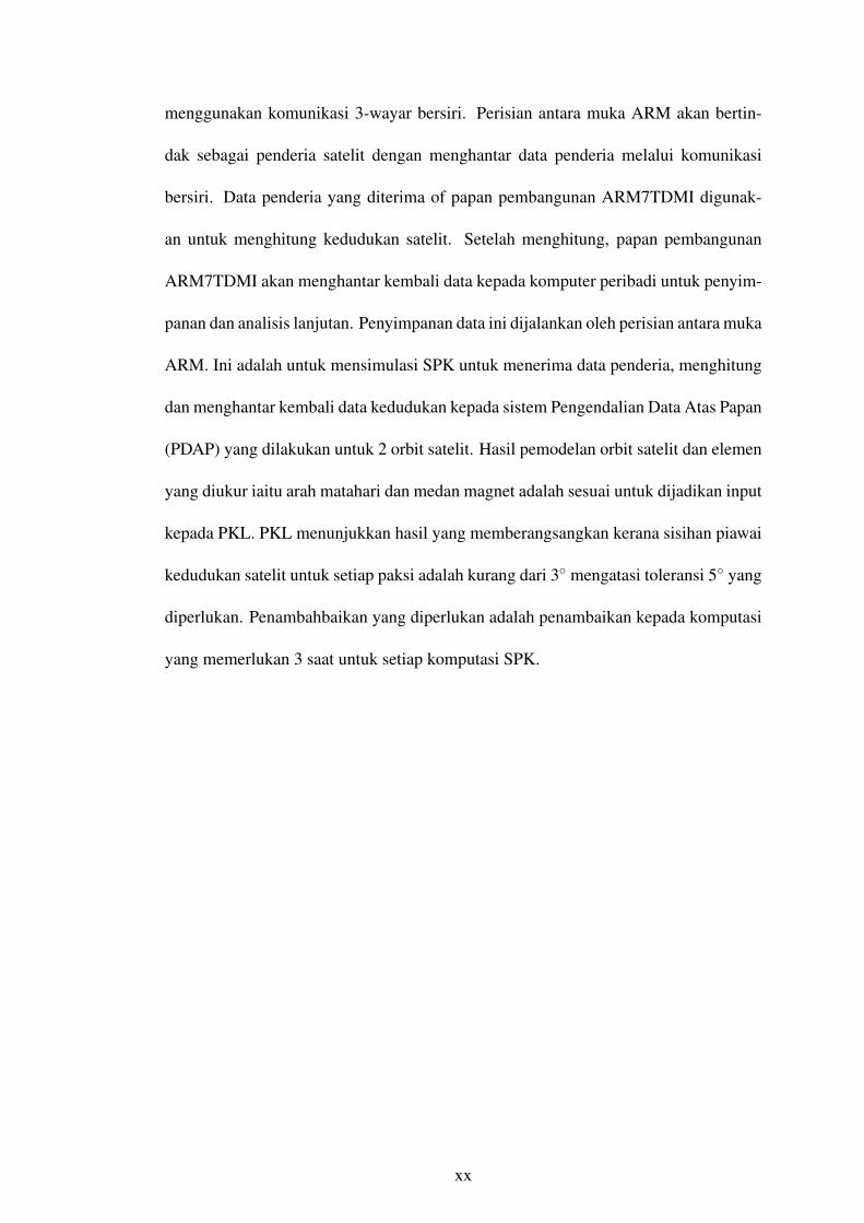
menggunakan komunikasi 3-wayar bersiri. Perisian antara muka ARM akan bertin-
dak sebagai penderia satelit dengan menghantar data penderia melalui komunikasi
bersiri. Data penderia yang diterima of papan pembangunan ARM7TDMI digunak-
an untuk menghitung kedudukan satelit. Setelah menghitung, papan pembangunan
ARM7TDMI akan menghantar kembali data kepada komputer peribadi untuk penyim-
panan dan analisis lanjutan. Penyimpanan data ini dijalankan oleh perisian antara muka
ARM. Ini adalah untuk mensimulasi SPK untuk menerima data penderia, menghitung
dan menghantar kembali data kedudukan kepada sistem Pengendalian Data Atas Papan
(PDAP) yang dilakukan untuk 2 orbit satelit. Hasil pemodelan orbit satelit dan elemen
yang diukur iaitu arah matahari dan medan magnet adalah sesuai untuk dijadikan input
kepada PKL. PKL menunjukkan hasil yang memberangsangkan kerana sisihan piawai
kedudukan satelit untuk setiap paksi adalah kurang dari 3 mengatasi toleransi 5 yang
diperlukan. Penambahbaikan yang diperlukan adalah penambaikan kepada komputasi
yang memerlukan 3 saat untuk setiap komputasi SPK.
xx
ATTITUDE DETERMINATION SYSTEM FOR NANO SATELLITE USING
EXTENDED KALMAN FILTER ON ARM7TDMI PLATFORM
ABSTRACT
Extended Kalman Filter (EKF) has been successfully utilized in satellites missions.
However, in comparison to other attitude determination methods developed, it is one of
the most computationally burdening algorithm and with the new development of using
nano satellites which have limited electrical power, mass, space and usually budget, it
is essential to design an Attitude Determination System (ADS) which conforms to this
limitation. Therefore, in this thesis, as a computational improvement on the InnoSAT
project, the RCM3400 microcontroller of the ADS is replaced with the ARM7TDMI
based microprocessor to test its capability. The ARM7TDMI has been chosen since
it is one of the well-known microprocessor used in various electronic equipment be-
cause it is low power and robust. The EMBEST S3CEV40 Development Board used,
houses the S3C44B0X microprocessor which is an ARM7TDMI microprocessor. The
testing is done by connecting the development board to a personal computer which
has been installed with the ARM Interface Software based on Visual Basic 6.0. The
development board is embedded with the ADS software based on the EKF. The com-
munication for the two system uses 3-wire serial communication. The ARM Interface
software will act as the sensor of the satellite by sending sensor data via serial com-
munication. Sensor data received by the ARM7TDMI development board is used to
calculate the attitude of the satellite. Once calculated, the ARM7TDMI development
xxi

board will send attitude data back to the PC for storage and further analysis. Data
storage is done by ARM Interface software. This is to simulate the ADS system to
receive sensor data, calculate and send back attitude data to On Board Data Handling
(OBDH) system which is done for 2 satellite orbits. Modelling results of satellite orbit
and sensed elements consisting of sun position and magnetic field are suitable to be
used for EKF input. The EKF shows promising results as the satellite attitude standard
deviation in each axis is less than 3 exceeding the 5 required tolerance. The only
improvement required is the computation which need 3 seconds for each computation
on ADS.
xxii
CHAPTER 1
INTRODUCTION
1.1 Background
InnoSAT satellite program is a satellite program lead by Astronautics Technology
Sdn. Bhd. (ATSB) and Malaysian National Space Agency (ANGKASA). InnoSAT is a
300×100×100mm3 or a 3 unit CubeSat nanosatellite design. CubeSat was collabora-
tively designed by California Polytechnic State University and Stanfords University’s
Space Systems Development Laboratory (Lee et al., 2009) to provide a standard design
for picosatellite to reduce cost and development time, increase accessibility to space,
and sustain frequent launches. Many institutions use this platform as their platform for
various mission. Some like the Danish AAUSAT-II uses the CubeSat satellite platform
for educational purposes and at the same time for research in gamma radiation in space
(Andresen et al., 2005). California Institute of Technology and National Aeronautics
and Space Administration (NASA) teamed up to design the CubeSat Hydrometric At-
mospheric Radiometer Mission (CHARM) satellite to be used for Earth radiometry
study which replaces the use of large and costly satellites (Lim et al., 2012). Dickin-
son et al. (2011) uses the CubeSat platform for their satellite to predict and diagnose
space weather events at Earth. Many researches have been done using the CubeSat
platform which is why the CubeSat is a suitable start off for InnoSAT as a new satellite
research in Malaysia. The program provides local universities with the opportunity
to be involved with a real satellite project with ATSB as the project leader as each
university takes part by developing a specific subsystem for InnoSAT.
1
1.2 Problem Statement
Universiti Sains Malaysia (USM) was given the opportunity to develop the Attitude
Determination System (ADS) of InnoSAT. ADS is one of the crucial subsystems of a
satellite. The satellite would be flying blindly and eventually out of control without
this subsystem. Thus USM took the opportunity to develop an ADS which has been
designated Space Experimental Attitude Determination System (SEADS) and a Rabbit
RCM3400 based microcontroller board which process sensor measurement to generate
InnoSAT attitude. SEADS consists of three sensors which has been installed on In-
noSAT. First sensor consists of 4 sets of three sided pyramidal sun sensors designated
Experimental Pyramidal Sun Sensor (ExPSS), second is a magnetometer designated
Experimental Earth Magnetic Field Probe (ExEMFP) and finally a redundant sun sen-
sor designated Solar Panel Sun Sensor (SPSS) which utilizes InnoSAT solar panels
to generate sun vector. All sensors provide sun position and magnetic field vector of
InnoSAT in Spacecraft Body Coordinate (SBC) frame.
Readings from the sensors are to be processed by the Rabbit RCM3400 micro-
controller board to be stored in an on board flash memory and to generate attitude of
InnoSAT. The Rabbit RCM3400 controller board has been embedded with an attitude
determination algorithm consisting of Kepler orbit model which generates InnoSAT
position vector in Earth Centered Inertial (ECI) frame, Keplerian sun model and In-
ternational Geomagnetic Reference Field (IGRF) model which generates the sun and
magnetic field vectors respectively in the ECI frame and a combination of Extended
Kalman filter (EKF) and Q-method which calculate InnoSAT attitude using both sun
and magnetic field vector in ECI and SBC frames.
2
Though, this was the plan for RCM3400 controller board, a combination of is-
sues surfaced during the implementation of the algorithm which are improper Julian
date representation, RCM3400 computation speed limit and memory burden of ADS.
The first issue is the Julian date. Julian date is a crucial initial parameter to the orbit
model where the orbit model is a crucial starting point for further attitude determina-
tion processing. However, during implementation of attitude determination methods in
Attitude Determination and Control System (ADCS) of InnoSAT, it is found that the
RCM3400 cannot represent Julian date variable accurately in 32 bits(floating point) but
should be represented in double 64 bit numbers, because the date precision exceed the
32 bit decimal limit causing major calculation errors. Another issue is the computation
speed limitation and memory burden of ADS on RCM3400 micro-controller. The EKF
with the inverse of element matrix larger than 3x3 and the IGRF calculation with an
order of 10 caused a significant overloading of RCM3400 memory and reduction in
processing time.
Therefore, in order to improve on the capabilities of InnoSAT ADS, an ARM7TDMI
microprocessor will be tested to see whether the capabilities of the ARM7TDMI would
be suitable for InnoSAT ADS.
1.3 Objective of study
From above, the objectives of this research are
(i) To estimate the attitude of InnoSAT from combination of two position sensors
using EKF
3
(ii) To embed the EKF attitude estimation algorithm in the ARM7TDMI based mi-
croprocessor
(iii) To compare the performance and result of the experimentation of the real time
embedded EKF with Satellite Toolkit (STK) software.
1.4 Scope and Limitations
The scope of this research is limited to the ADS of InnoSAT only. Though a real
satellite would include a control system, which completes the ADCS of a full satellite,
adding the control system to the research would be too big for this research. Testing
would only be done to the microprocessor by using a development board on ground.
Sensor readings are simulated readings from STK by using proposed InnoSAT Two
Line Element (TLE) provided by ATSB.
1.5 Thesis Organization
This thesis is divided into 5 chapters which entails the implementation EKF based
ADS on ARM7TDMI. Chapter 1 introduces InnoSAT which is the satellite platform
and base for this research. Research goals and overview is also included in this chap-
ter. Chapter 2 presents a literature review of ADS used by various groups around
the world. The fundamentals of ADS and EKF are also explained in this section as
well space requirement of a satellite system. Chapter 3 presents the method of ex-
perimentation for the implementation of the EKF on the ARM7TDMI microprocessor.
Chapter 4 discusses the results of the implementation of the EKF based ADS on the
ARM7TDMI microprocessor. Finally, Chapter 5 concludes the finding of this thesis
and the recommendations for future work.
4
CHAPTER 2
OVERVIEW OF ATTITUDE DETERMINATION SYSTEM AND
ARCHITECTURE
2.1 Introduction
Attitude of a spacecraft is its orientation in space. Attitude determination is the
process of computing the orientation of the spacecraft relative to either an inertial ref-
erence or some object of interest, such as Earth. This typically involves several types
of sensors on each spacecraft and sophisticated data processing procedures (Wertz,
1978).
2.2 Attitude Determination System Architectures
Satellite subsystems are unique to one another. This is also true for the ADS. The
configuration and combination of sensors and the built in electronic system depends
on the mission, satellite size and shape.
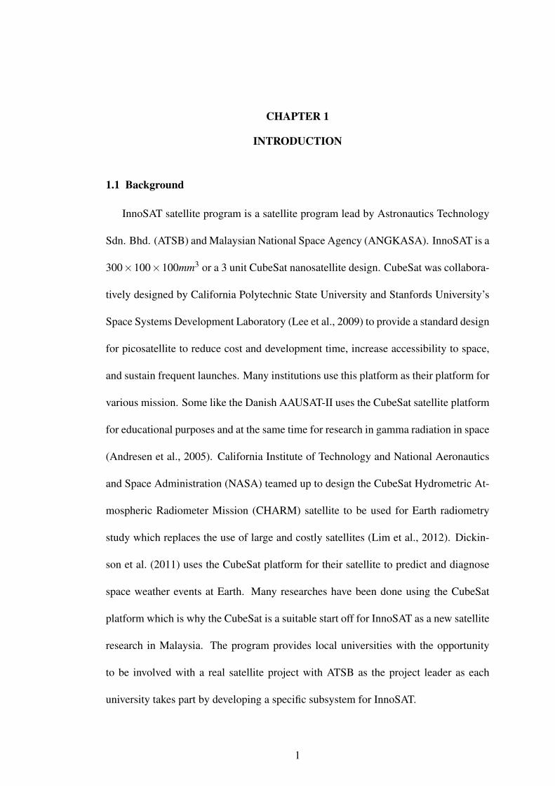
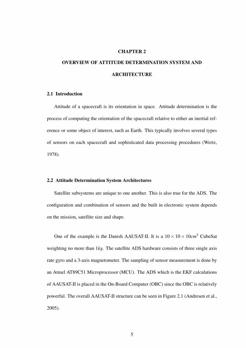
One of the example is the Danish AAUSAT-II. It is a 10× 10× 10cm3 CubeSat
weighting no more than 1kg. The satellite ADS hardware consists of three single axis
rate gyro and a 3-axis magnetometer. The sampling of sensor measurement is done by
an Atmel AT89C51 Microprocessor (MCU). The ADS which is the EKF calculations
of AAUSAT-II is placed in the On-Board Computer (OBC) since the OBC is relatively
powerful. The overall AAUSAT-II structure can be seen in Figure 2.1 (Andresen et al.,
2005).
5
1.3. AAUSAT-II SUBSYSTEMS
P/LEPS
MCCGND
COM
MECH
Earth
Satellite
ADCS
OBC
CDH
Radio Link
AX.25
CAN bus
TCP
Figure 1.1: Block diagram depicting the subsystems in theAAUSAT-II and a conceptual visualization of their respective in-terfaces to other subsystems.
1.3.2 Subsystem Descriptions
MCC (Mission Control Center) is responsible for handling and storing all transmission data from the satel-lite and sending flight plans etc. to the satellite. The MCC provides a user interface and a database tostore housekeeping data from the satellite. The mission control center is furthermore able to controlmultiple ground stations, both the ground station located in Aalborg and a ground station placed atSvalbard in Norway which is currently in the final stages of developement.
GND (Ground Station) is responsible for the communication between the MCC and the satellite. The task ofthe ground station is to track the satellite throughout each pass and adjust the radio frequency, so databetween the satellite and the MCC can be sent and received correctly. Furthermore, the ground stationis designed to be autonomously controlled by the MCC, both for communicating with the AAUSAT-IIsatellite and the ESA SSETI Express satellite2.
COM (Communication System) is designed to function as a pipeline for the communication between theground station and the CDH. COM modulates and sends data from CDH to the ground station. Datareceived from the ground station is demodulated and sent via the CAN bus to the CDH subsystem.
EPS (Electrical Power Supply) is responsible for generating power from the solar cells and storing it in thebatteries in order to be able to deliver continuous power during eclipse and peak demands. The EPSsubsystem also conditions and distributes the power to other satellite subsystems.
ADCS (Attitude Determination and Control System) is responsible for determining and controlling the at-titude of the satellite. This primarily implies detumbling and stabilization of the satellite.
P/L (Payload) consists of a gamma ray burst detector. The gamma ray burst detector is a newly developeddetector crystal supplied by Danish National Space Center.
OBC (On-Board Computer) is the main computer on the satellite. The CDH subsystem software is executedon the OBC. The OBC subsystem also provides processing facilities for other satellite subsystems.
2http://sseti.gte.tuwien.ac.at/WSW4/express1.htm
10
Figure 2.1: AAUSAT-II overall satellite structure (Andresen et al., 2005)
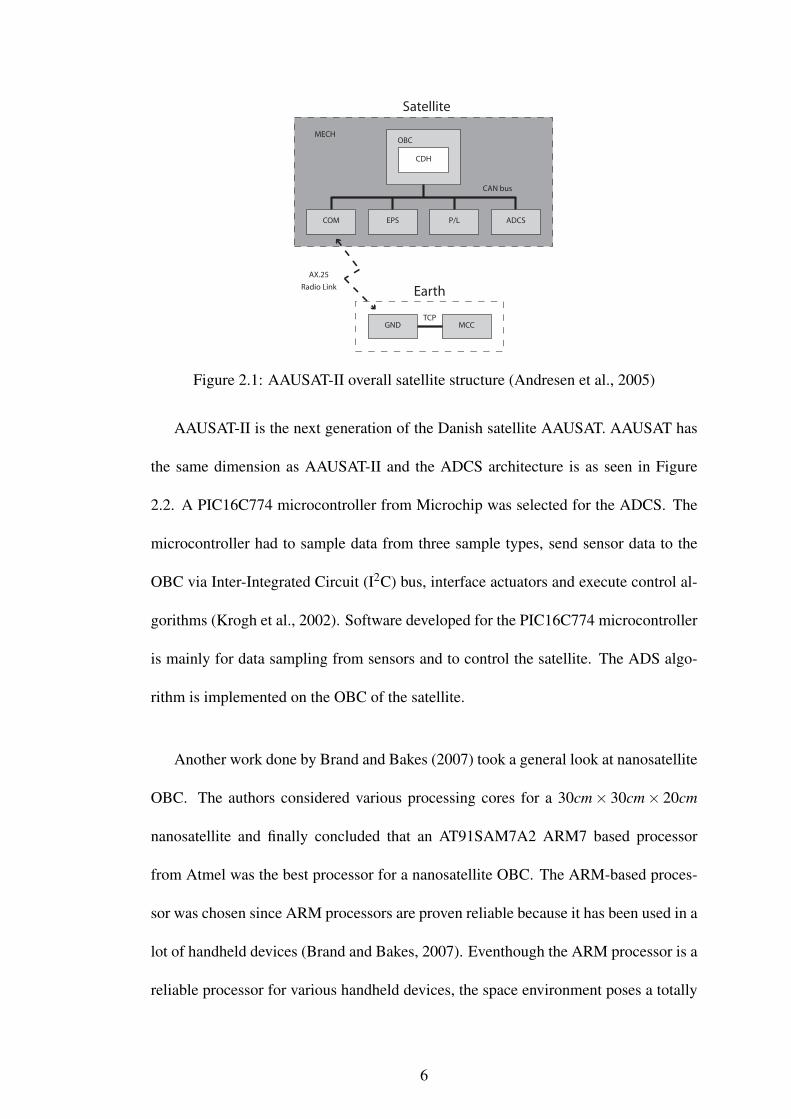
AAUSAT-II is the next generation of the Danish satellite AAUSAT. AAUSAT has
the same dimension as AAUSAT-II and the ADCS architecture is as seen in Figure
2.2. A PIC16C774 microcontroller from Microchip was selected for the ADCS. The
microcontroller had to sample data from three sample types, send sensor data to the
OBC via Inter-Integrated Circuit (I2C) bus, interface actuators and execute control al-
gorithms (Krogh et al., 2002). Software developed for the PIC16C774 microcontroller
is mainly for data sampling from sensors and to control the satellite. The ADS algo-
rithm is implemented on the OBC of the satellite.
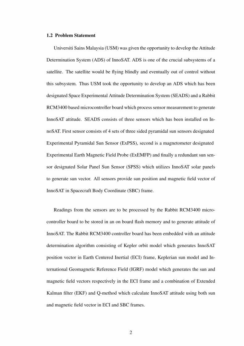
Another work done by Brand and Bakes (2007) took a general look at nanosatellite
OBC. The authors considered various processing cores for a 30cm× 30cm× 20cm
nanosatellite and finally concluded that an AT91SAM7A2 ARM7 based processor
from Atmel was the best processor for a nanosatellite OBC. The ARM-based proces-
sor was chosen since ARM processors are proven reliable because it has been used in a
lot of handheld devices (Brand and Bakes, 2007). Eventhough the ARM processor is a
reliable processor for various handheld devices, the space environment poses a totally
6
different threat to a satellite when compared with the Earth’s environment. Brand and
Bakes’s main concern are errors caused by radiation exposure in the space since the
chosen processor is not a space qualified component. However, in recent years, satel-
lite developers has begun experimenting and using Commercial of The Shelf (COTS)
components which include processors as well. Eventhough these COTS components
are susceptible to radiation errors, they are much cheaper compared to space quali-
fied components. Brand and Bakes (2007)’s also suggest that the vital part which is
the onboard memory the satellite should consists only of static random-access mem-
ory (SRAM) and flash memory only with the inclusion of some form of detection
and correction hardware. According to the authors as well, the most computationally
complex operation a nanosatelite would have to deal with using its limited hardware
is the IGRF modelling of ADCS. This confirms the high computation of the IGRF
modelling.
Figure 2.2: AAUSAT overall satellite structure (Brand and Bakes, 2007)
nCUBE is a Norwegian student satellite (Ose, 2004). It is in the same league as
both AAUSAT satellite in terms of size and weight. The ADS or the attitude estimator
also uses an EKF which is written in C programming language. The nCUBE team
7
chose an ATmega128L since it is the low power version. Ose (2004) also realized that
EKF requires highly accurate variables, therefore the variables of the EKF in AAUSAT
program is implemented as floating variables which has a range of ±3.403× 10308
and an accuracy of ±1.175× 10−308 (IEEE Std 754-2008, 2008; 754-1985, 1985).
This also indicates the ATmega128L microcontroller is able to use variables in double
precision format.
The CubeSat Heliospheric Imaging Experiment (CHIME) satellite as mentioned
by Dickinson et al. (2011) uses a Gumstix Verdex computer for its OBC which also
govern the attitude determination and control of CHIME. The CHIME satellite uses
two sun sensors to determine its attitude.
Another architecture done by Ali et al. (2014) into the AraMiS-C1 satellite, is the
integration of the Electric Power Supply (EPS) and the ADCS onto a single Cubesat
standard tile. The AraMiS-C1 satellite system uses COTS components. Sensors on
board consists of sun detector and magnetometer. System management of the satellite
is done by a commercial MSP430F5438A ultra power 16-bit Reduced Instruction Set
Computing (RISC) architecture microcontroller which support up to 25Mhz system
clock.
Yang et al. (2012) used a TMS320C54 series Digital Signal Processor (DSP) from
Texas Instruments to perform the duty of controller by implementing sampling, com-
puting and actuating algorithms. The system performs a dual-vector attitude deter-
mination based on solar and Earth-magnetic sensor reading. The ADCS manages to
stabilize the satelite the attitude with Earth-pointing precision of 5circ when the sun in
8
visible.
2.3 Satellite Orbit Description
A satellite orbiting the Earth is considered a two point mass which are influenced by
their mutual gravitational attraction (Jensen et al., 2010). This system can be described
by using Kepler’s three empirical laws of planetary motion (Wertz, 1978).
2.3.1 Keplerian Orbit
An orbit can be described using the method developed by Johannes Kepler which
gives a description of the orbit size, shape and orientation, as well a spacecraft’s posi-
tion (Sellers et al., 2003). The method requires only 6 orbital elements which are:
• Semimajor axis, as
• Eccentricity, es
• Inclination, is
• Right Ascension of Ascending Node (Ωs)
• Argument of Perigee, ωs
• True Anomaly, νs
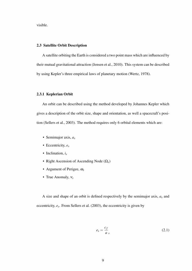
A size and shape of an orbit is defined respectively by the semimajor axis, as and
eccentricity, es. From Sellers et al. (2003), the eccentricity is given by
es =c f
a s(2.1)
9
where c f is the distance from the ellipse center to the ellipse focal point (Earth) as
in Figure 2.3.
Figure 2.3: Geometric properties of an elliptical orbit with the Earth as focal point
The shape of the orbit either a circle, ellipse, parabola or a hyperbola depends on
the eccentricity, es and the relationship can be seen in Table 2.1.
Table 2.1: Orbit shape relationship with eccentricity
Orbit Shape EccentricityCircle es = 0Ellipse 0 < es < 1Parabola es = 1Hyperbola es > 0
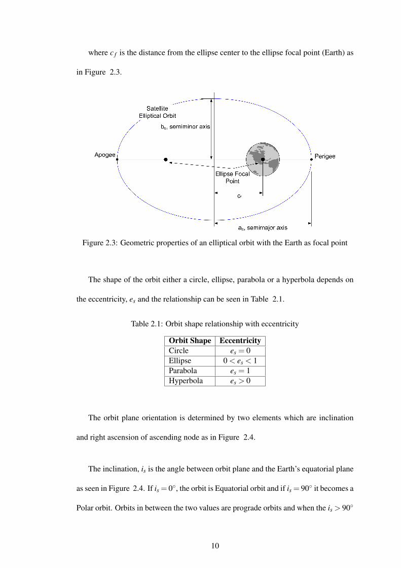
The orbit plane orientation is determined by two elements which are inclination
and right ascension of ascending node as in Figure 2.4.
The inclination, is is the angle between orbit plane and the Earth’s equatorial plane
as seen in Figure 2.4. If is = 0, the orbit is Equatorial orbit and if is = 90 it becomes a
Polar orbit. Orbits in between the two values are prograde orbits and when the is > 90
10
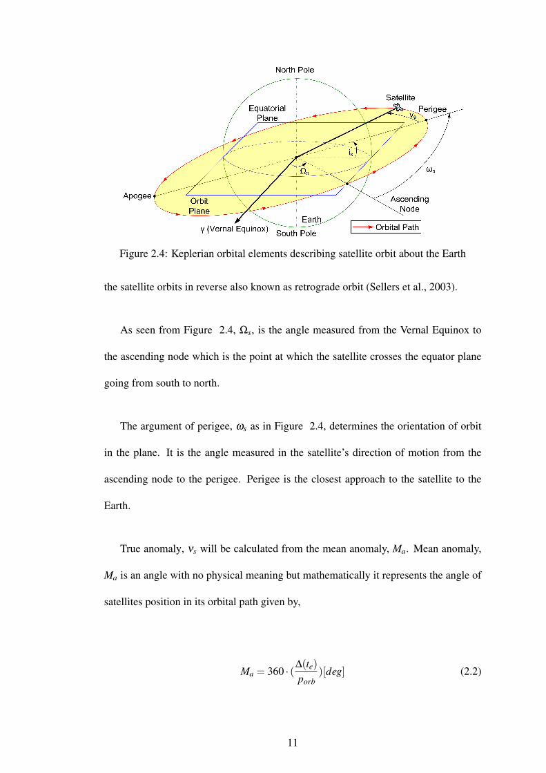
Figure 2.4: Keplerian orbital elements describing satellite orbit about the Earth
the satellite orbits in reverse also known as retrograde orbit (Sellers et al., 2003).
As seen from Figure 2.4, Ωs, is the angle measured from the Vernal Equinox to
the ascending node which is the point at which the satellite crosses the equator plane
going from south to north.
The argument of perigee, ωs as in Figure 2.4, determines the orientation of orbit
in the plane. It is the angle measured in the satellite’s direction of motion from the
ascending node to the perigee. Perigee is the closest approach to the satellite to the
Earth.
True anomaly, νs will be calculated from the mean anomaly, Ma. Mean anomaly,
Ma is an angle with no physical meaning but mathematically it represents the angle of
satellites position in its orbital path given by,
Ma = 360 · (∆(te)porb
)[deg] (2.2)
11
where:
∆(te) is the time difference between the epoch and the last perigee passage before
epoch and porb is the orbital period.
Figure 2.5: Relationship between True Anomaly and Eccentric Anomaly
Mean anomaly is linked to the true anomaly by an intermediate variable, the Eccen-
tric anomaly, Ea which can be seen in Figure 2.5. The mean and eccentric anomalies
are related by Kepler’s equation as
Ma = Ea− es sinEa (2.3)
12
Then Gauss’s equation relates the eccentric anomaly to the True Anomaly, νs by
tan(νs
2)=
(1+ es
1− es
)1/2
tan(Es
2)
(2.4)
From Equation 2.4, True Anomaly, νs can be expressed directly as a function of
Mean Anomaly, Ma by expanding in a power series in orbital Eccentricity, es to yield
νs = Ma +2es sin(Ma)+5e2s
sin(2Ma)
4(2.5)
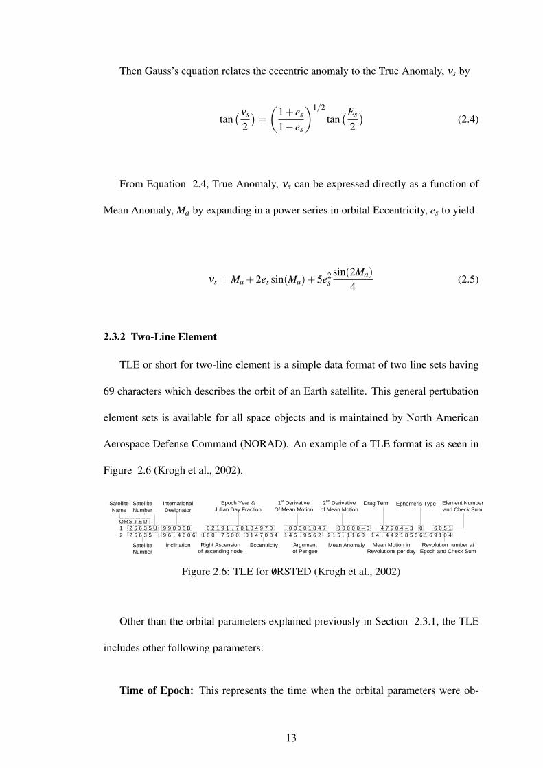
2.3.2 Two-Line Element
TLE or short for two-line element is a simple data format of two line sets having
69 characters which describes the orbit of an Earth satellite. This general pertubation
element sets is available for all space objects and is maintained by North American
Aerospace Defense Command (NORAD). An example of a TLE format is as seen in
Figure 2.6 (Krogh et al., 2002).
O R S T E D1 2 5 6 3 5 U 9 9 0 0 8 B 0 2 1 9 1 . 7 0 1 8 4 9 7 0 . 0 0 0 0 1 8 4 7 0 0 0 0 0 – 0 4 7 9 0 4 – 3 0 6 0 5 12 2 5 6 3 5 9 6 . 4 6 0 6 1 8 0 . 7 5 0 0 0 1 4 7 0 8 4 1 4 5 . 9 5 6 2 2 1 5 . 1 1 6 0 1 4 . 4 4 2 1 8 5 5 6 1 6 9 1 0 4
SatelliteNumber
InternationalDesignator
Epoch Year &Julian Day Fraction
1st DerivativeOf Mean Motion
2nd Derivativeof Mean Motion
Drag Term Ephemeris Type Element Numberand Check Sum
SatelliteNumber
Inclination Right Ascensionof ascending node
Eccentricity Argumentof Perigee
Mean Anomaly Mean Motion inRevolutions per day
Revolution number at Epoch and Check Sum
SatelliteName
Figure 2.6: TLE for /0RSTED (Krogh et al., 2002)
Other than the orbital parameters explained previously in Section 2.3.1, the TLE
includes other following parameters:
Time of Epoch: This represents the time when the orbital parameters were ob-
13

tained. Epoch year in described in the first two numbers. The remaining numbers in
the integral part is the Julian day and the fraction represent the fractional portion of the
day.
1st Derivative of Mean Motion: This represents the change in the mean motion
of the satellite. It is the half value of the mean motion in revolutions per day squared
and is caused by atmospheric drag pulling a satellite into a lower orbit and accelerates
it downward towards the Earth.
2nd Derivative of Mean Motion: This term is the 2nd second derivative of the
mean motion divided by six, in units of revolutions per day cubed and is usually set
to zero since it is not used because the orbit model only considers the force of Earth’s
gravity acting on the satellite for estimation.
Drag Term: A drag term or radiation pressure coefficient consists of a coefficient
describing the effect of drag on a satellite. It is based on a satellite surface and mass.
Mean Motion: Mean motion describes the number of revolution a satellite com-
pletes in day.
Revolution Number at Epoch: This parameter gives the number of orbit at the
Epoch time when TLE was taken.
2.3.3 Julian Date
A very useful and common representation of time which simplifies astronomical
calculation and satellite orbit propagation is the Julian date. It is counted in day plus a
14
fraction of the day beginning at noon universal time. It has been counted in days since
1st of January 4713 BC at noon universal time (Wertz, 1978; Danby, 1988; Sinnott,
1991).
The Julian date used in this research will not use the entire Julian date from 1st
January 4713BC noon but instead will use the Julian date starting from noon UTC on
the 1st January 2000. This will offset the Julian date by 2451545 days subtracted from
the ordinary Julian date.
2.3.4 Orbit Model
Having known the orbit of a satellite, at a certain point and time from a TLE, it is
also required to determine the position and motion of a satellite in order to determine
the attitude of a satellite. A simple two body Keplerian orbit propagator model devel-
oped by the AAUSAT team will be used (Krogh et al., 2002). This orbit model will
use the orbital and time parameters from a given TLE.
The first step of the orbit model is to determine the current mean anomaly of the
satellites orbital position. The time since epoch, Tse is used here. It is the current
time in Julian date minus the Julian date at Epoch given in the TLE. The current
Mean Anomaly, Ma is calculated in degrees using Equation 2.6, which includes mean
anomaly at epoch, ME poch and the mean motion, nrev from the TLE.
Ma = ME poch +360nrevTse (2.6)
15
The semi major axis, as which represent the largest radius of an eccentric orbit as
shown in Figure 2.3 is given by
as =
(mg
(2nrevπ
86400 )2
)1/3
(2.7)
Next the daily changes of Argument of Perigee, ωs and daily changes of the Right
Ascension of Ascending Node, Ωs is determined since the Argument of Perigee, ωs and
Ωs changes with a constant speed relative to the ECI frame is determined. Parameters
used in the determination are orbital Inclination, is, the orbital Eccentricity, es, Semi
Major Axis of the orbit, as and the Earth’s Equatorial Radius, rearth (Krogh et al., 2002;
Wertz, 1978).
ωs = 4.98204((rearth
as)3.5)(5cos(is)2−1)((1− e2
s )2)−1 (2.8)
Ωs = 9.9641((rearth
as)3.5)cos(is)((1− e2
s )2)−1 (2.9)
Accordingly the current Argument of Perigee, ωs and the Ωs can now be deter-
mined by updating the same parameters given in the TLE parameters, ωs,T LE and
Ωs,T LE with ωs and Ωs resulting in
ωs = ωs,T LE +Tseωs (2.10)
16
Ωs = Ωs,T LE −TseΩs (2.11)
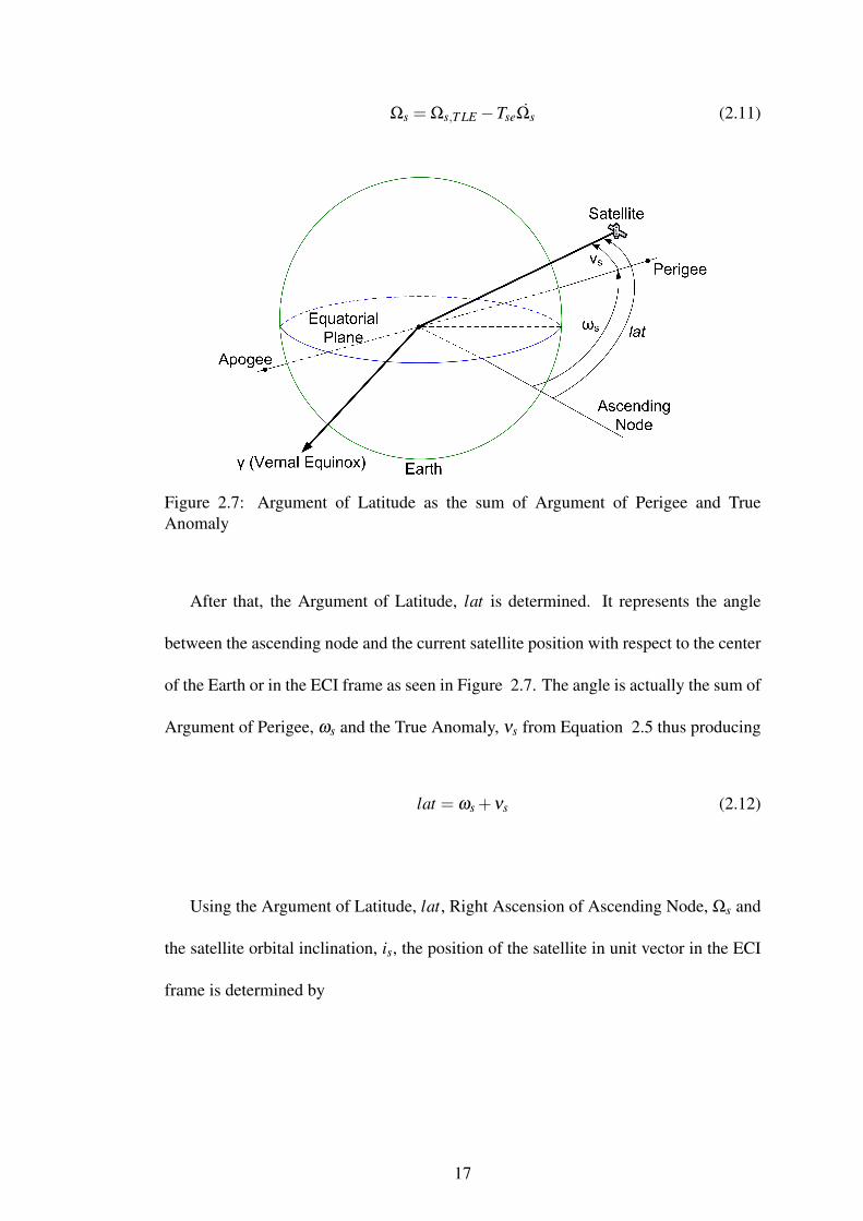
Figure 2.7: Argument of Latitude as the sum of Argument of Perigee and TrueAnomaly
After that, the Argument of Latitude, lat is determined. It represents the angle
between the ascending node and the current satellite position with respect to the center
of the Earth or in the ECI frame as seen in Figure 2.7. The angle is actually the sum of
Argument of Perigee, ωs and the True Anomaly, νs from Equation 2.5 thus producing
lat = ωs +νs (2.12)
Using the Argument of Latitude, lat, Right Ascension of Ascending Node, Ωs and
the satellite orbital inclination, is, the position of the satellite in unit vector in the ECI
frame is determined by
17
xsat = cos(lat)cos(Ωs)− sin(lat)sin(Ωs)cos(is)
ysat = cos(lat)sin(Ωs)+ sin(lat)cos(Ωs)cos(is)
zsat = sin(lat)sin(is)
(2.13)
To give a measurable figure to the orbital position of the satellite position in kilometers,
the position vector in Equation 2.13 is multiplied with the radius of the satellites orbital
position, rsat(in kilometers) as below
rsat = as1− e2
s1+ es cos(νs)
(2.14)
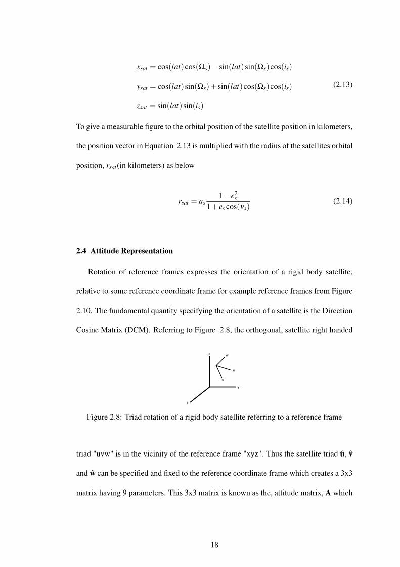
2.4 Attitude Representation
Rotation of reference frames expresses the orientation of a rigid body satellite,
relative to some reference coordinate frame for example reference frames from Figure
2.10. The fundamental quantity specifying the orientation of a satellite is the Direction
Cosine Matrix (DCM). Referring to Figure 2.8, the orthogonal, satellite right handed
u
v
w
x
y
z
Figure 2.8: Triad rotation of a rigid body satellite referring to a reference frame
triad "uvw" is in the vicinity of the reference frame "xyz". Thus the satellite triad u, v
and w can be specified and fixed to the reference coordinate frame which creates a 3x3
matrix having 9 parameters. This 3x3 matrix is known as the, attitude matrix, A which
18
is
A≡
ux uy uz
vx vy vz
wx wy wz
(2.15)
with u = (ux,uy,uz)T , v = (vx,vy,vz)
T and w = (wx,wy,wz)T . Each of the elements is
a cosine of the angle between a body unit vector and a reference axis. For example, the
cosine of the angle between v and reference y-axis is represented by vy. Due to this, A
is referred to as DCM.
A DCM is a coordinate transformation (Wertz, 1978) that maps vectors from a
reference frame to the body frame where if a is a vector with components a1, a2 and
a3 along the reference axes, then
Aa =
ux uy uz
vx vy vz
wx wy wz
a1
a2
a3
=
u ·a
v ·a
w ·a
≡
au
av
aw
(2.16)
The components of Aa are the components of the vector a along the body triad u, v, and
w. Other than the DCM, there are other parameterizations that specifies the orientation
of a rigid. However, in this thesis, the Euler angles and the Euler Symmetric Parameters
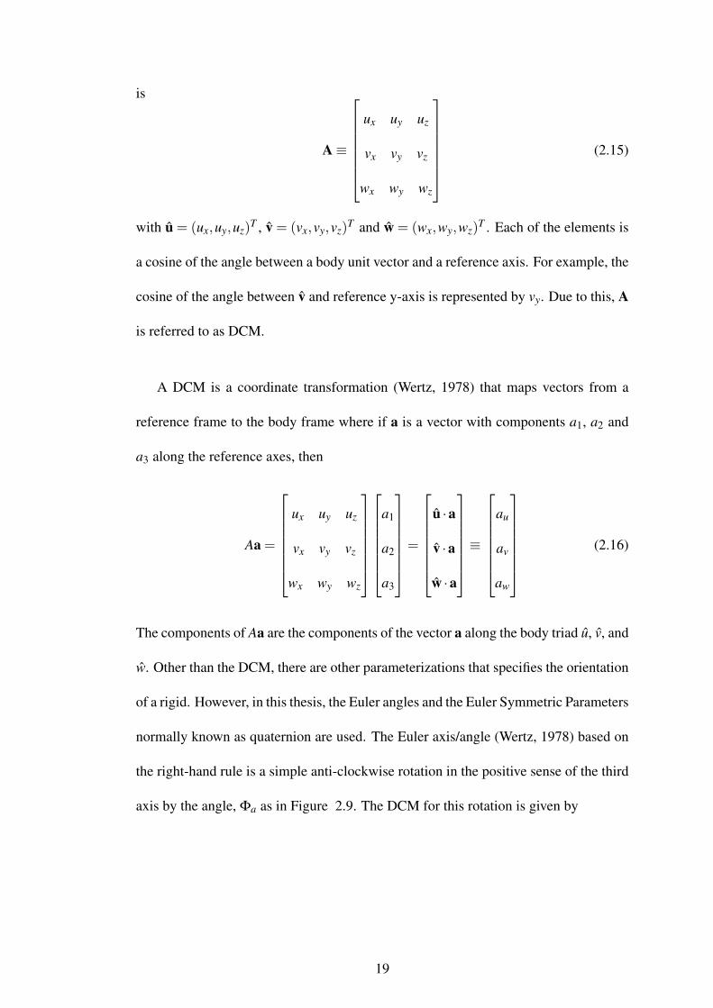
normally known as quaternion are used. The Euler axis/angle (Wertz, 1978) based on
the right-hand rule is a simple anti-clockwise rotation in the positive sense of the third
axis by the angle, Φa as in Figure 2.9. The DCM for this rotation is given by
19
A3(Φa) =
cosΦa sinΦa 0
−sinΦa cosΦa 0
0 0 1
(2.17)
Figure 2.9: Rotation about the third axis with angle Φa (Wertz, 1978)
The DCM rotation in the first and second axis by the angle, Φa is represented by
A1(Φa) and A2(Φa), respectively and they are
A1(Φa) =
1 0 0
0 cosΦa sinΦa
0 −sinΦa cosΦa
(2.18)
A2(Φa) =
cosΦa 0 −sinΦa
0 1 0
sinΦa 0 cosΦa
(2.19)
All three matrices have the trace
tr(A(Φa)) = 1+2cosΦa (2.20)
20
The trace of a DCM representing a rotation by an angle, Φa about an arbitrary axis
takes the same value. Generally, the axis rotation from one reference frame to another
reference frame might not be one of the ’xyz’ orthogonal axes but might be a unit
vector, e and an angle of rotation, Φa which results with a general DCM as
A =
cosΦa + e2
1(1− cosΦa) e1e2(1− cosΦa)+ e3 sinΦa e1e3(1− cosΦa− e2 sinΦa)
e1e2(1− cosΦa)− e3 sinΦa cosΦa + e22(1− cosΦa) e2e3(1− cosΦa)+ e1 sinΦa
e1e3(1− cosΦa)+ e2 sinΦa e2e3(1− cosΦa)− e1 sinΦa cosΦa + e23(1− cosΦa)
(2.21)
(Wertz, 1978)
Using the same principal with a unit vector along rotation axis, e and an angle
of rotation, Φa a set of four parameters known as the Euler symmetric parameter or
quaternion can be introduced to represent rotation of a rigid body and they are(Wertz,
1978)
q1 ≡ e1 sinΦa
2(2.22)
q2 ≡ e2 sinΦa
2(2.23)
q3 ≡ e3 sinΦa
2(2.24)
q4 ≡ cosΦa
2(2.25)
These four parameters are not independent but satisfy the constraint equation (Wertz,
1978)
q21 +q2
2 +q23 +q2
4 = 1 (2.26)
21
The quaternion DCM is given by
A(q) =
q2
1−q22−q2
3 +q24 2(q1q2 +q3q4) 2(q1q3−q2q4)
2(q1q2−q3q4) −q21 +q2
2−q23 +q2
4 2(q2q3 +q1q4)
2(q1q3 +q2q4) 2(q2q3−q1q4) −q21−q2
1 +q23 +q2
4
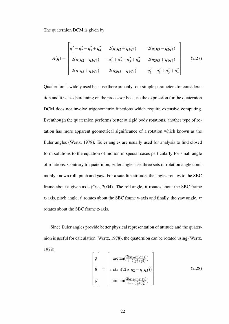
(2.27)
Quaternion is widely used because there are only four simple parameters for considera-
tion and it is less burdening on the processor because the expression for the quaternion
DCM does not involve trigonometric functions which require extensive computing.
Eventhough the quaternion performs better at rigid body rotations, another type of ro-
tation has more apparent geometrical significance of a rotation which known as the
Euler angles (Wertz, 1978). Euler angles are usually used for analysis to find closed
form solutions to the equation of motion in special cases particularly for small angle
of rotations. Contrary to quaternion, Euler angles use three sets of rotation angle com-
monly known roll, pitch and yaw. For a satellite attitude, the angles rotates to the SBC
frame about a given axis (Ose, 2004). The roll angle, θ rotates about the SBC frame
x-axis, pitch angle, φ rotates about the SBC frame y-axis and finally, the yaw angle, ψ
rotates about the SBC frame z-axis.
Since Euler angles provide better physical representation of attitude and the quater-
nion is useful for calculation (Wertz, 1978), the quaternion can be rotated using (Wertz,
1978) φ
θ
ψ
=
arctan(2(q1q4+q2q3)
1−2(q21+q2
2))
arctan(2(q4q2−q1q3))
arctan(2(q3q4+q2q1)
1−2(q22+q2
3))
(2.28)
22

2.5 Coordinate Frames
This section describes the frames used for determining the attitude in three di-
mensional space. The frames are important as the points on a rigid body is different
depending on different coordinate frames thus the correct reference frame has to be
known in all conditions. The method to rotate from the ECI frame to the Earth Cen-
tered Earth Fixed (ECEF) frame is also introduced in this section.
2.5.1 Reference Coordinate Frame
Since InnoSAT orbits the Earth, two specific Earth related coordinate system will
be used. They are the ECI and ECEF coordinate frame which have their origin in the
geographical center of Earth as shown in Figure 2.10.
X
Z
Y
Direction of Vernal Equinox
Equator
Rotation Axis
X
Z
Y
0 Longitude(Greenwich Line)
Equator
Rotation Axis
Figure 2.10: The ECI and ECEF coordinate frame
The first coordinate frame, Earth Centered Inertial represents a coordinate system
with its origin in the center of Earth and is fixed relative to the Earth rotation. The
X-axis is parallel to the direction of Vernal Equinox. The Vernal Equinox is the point
where the plane of the Earth’s orbit about the Sun, crosses the equator going from
23

South to North. The Z-axis is parallel to the Earth’s rotational axis.
The second Earth coordinate frame, the Earth Centered Earth Fixed frame has a
similar origin and Z-axis as the ECI frame but with a different X-axis. The X-axis,
stays and intersect the zero longitude of Earth designated the Greenwich Meridian
which fixes the ECEF frame to Earth thus, the system rotates with it.
2.5.2 Spacecraft Coordinate Frame
The satellite itself requires a set of fixed coordinate frames for attitude determina-
tion of the satellite. The attitude and position of the satellite is accordingly given as a
rotation between the satellite fixed coordinate frames and reference frames.
First is the SBC which is placed in the center of mass of the satellite and fixed to
the satellite geometric axes.The axis representation can be seen in Figure 2.11.
Figure 2.11: Spacecraft Body Coordinate for InnoSAT satellite
24


![Bohner Attitude Attitude Change 2011[1]](https://img.pdfslide.us/doc/110x75/577cdc9c1a28ab9e78aaef04/bohner-attitude-attitude-change-20111.jpg)


![Libraries] Function of Attitude Similarity and Attitude](https://img.pdfslide.us/doc/110x75/62e4a200fe037104c8733690/libraries-function-of-attitude-similarity-and-attitude-.jpg)