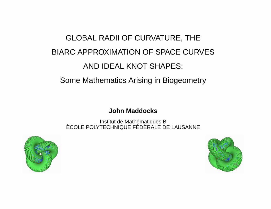
GLOBAL RADII OF CURVATURE, THE

BIARC APPROXIMATION OF SPACE CURVES

AND IDEAL KNOT SHAPES:

Some Mathematics Arising in Biogeometry

John Maddocks

Institut de Mathematiques BECOLE POLYTECHNIQUE FEDERALE DE LAUSANNE

In these three talks I will describe three ideas all pertaining to the analysis and

computation of optimal packings of cylindrical tubes centred on arbitrary space

curves. While I will not mention the specific applications in any detail, the

problem of cylindrical tubes, or fattened lines, arises in a variety of biological

contexts, for example packing of DNA into the capsid head of bacteriophages,

and the helical form of many bacteria and other simple organisms.

2

The first idea is that of global radius of curvature, which is a method of charac-

terizing the normal injectivity radius (or informally thickness) of a given space

curve.

3

The second idea is that of biarcs, which are a way of approximating arbitrary

space curves with arcs of circles. The biarc discretization combines very well

with the approach of global radius of curvature in the computation of thickness.

4

The third idea is the specific optimal packing problem of ideal knot shapes.

Here I will explain the problem, and then show approximately ideal shapes of

trefoil and figure-eight knots that were computed via a Monte Carlo code that

exploits global radius of curvature and the biarc discretization.

5

Joint Work:

JHM + Oscar Gonzalez, UT-Austin

JHM + OG + Heiko von der Mosel, Aachen + Friedemann Schuricht, Cologne

JHM + OG + Jana Smutny

JS, PhD Thesis, EPFL 2004 (and the majority of these slides)

JHM + JS + Mathias Carlen, Diplomant, EPFL + Ben Laurie, London

JHM + Andrzej Stasiak, U. of Lausanne

Crucial input from: Remi Langevin, U. of Bourgogne, Arieh Iserles, U. of Cam-

bridge

6

Plan of Course:

· Lecture 0: Some motivation (and the only biology...)

· Lecture 1: Global radii of curvature, thickness and normal injectivity radius

· Lecture 2: The biarc discretisation of space curves

· Lecture 3: Computations of ideal knot shapes

7

Lecture 0:

Many problems in biology and elsewhere involve tubular objects,

i.e., objects that can be modelled as volumes that can be de-

scribed as a three dimensional curve with a positive thickness

obtained by translating along the curve a constant radius circle in

the normal plane.

For example.....

8

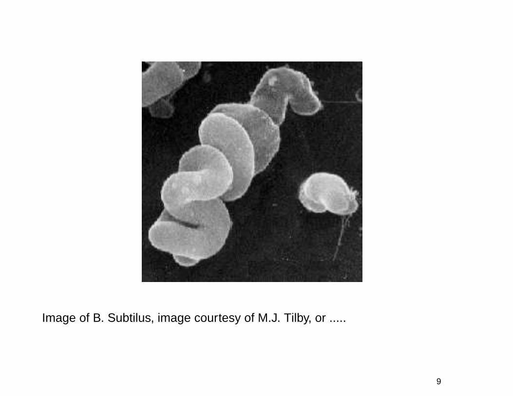
Image of B. Subtilus, image courtesy of M.J. Tilby, or .....

9

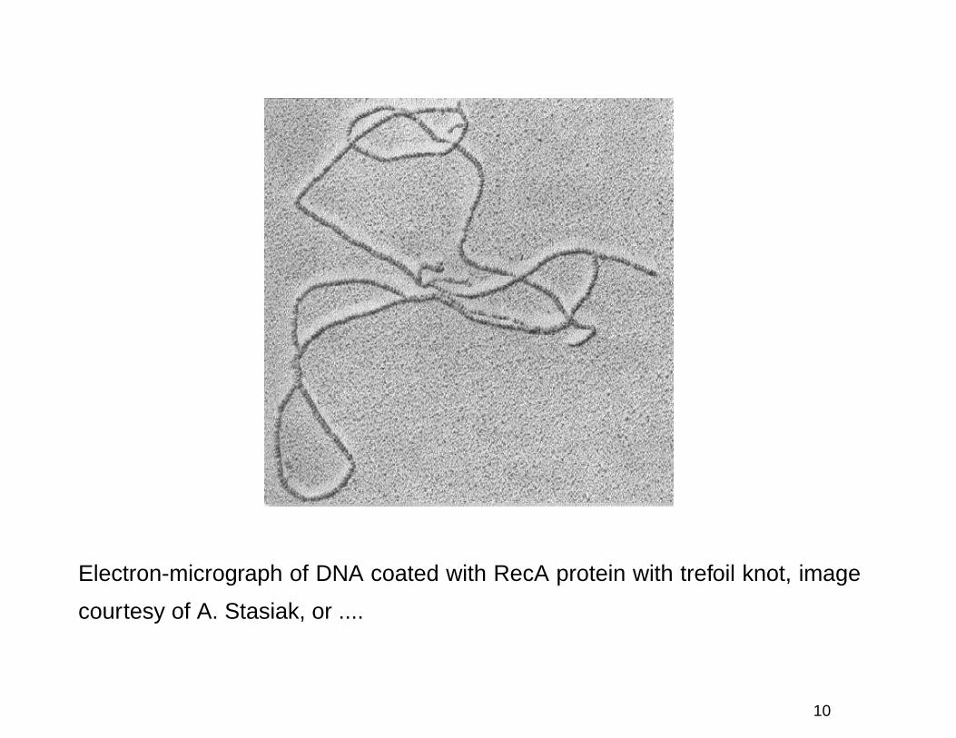
Electron-micrograph of DNA coated with RecA protein with trefoil knot, image

courtesy of A. Stasiak, or ....

10

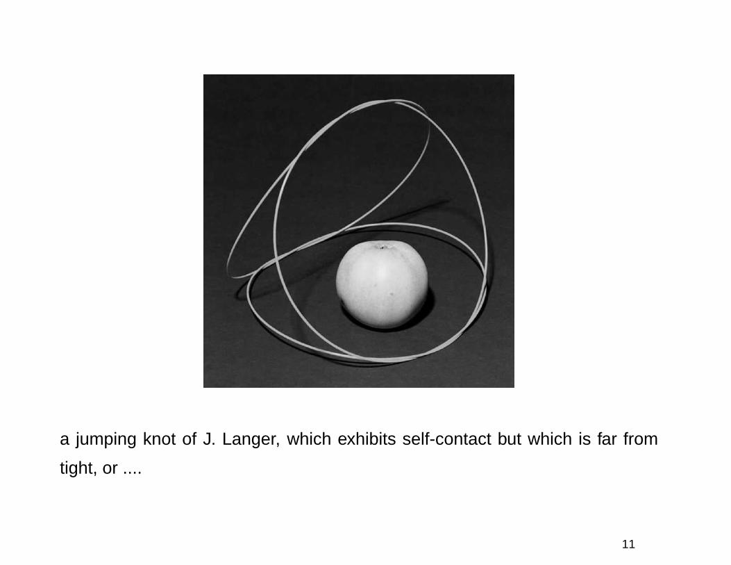
a jumping knot of J. Langer, which exhibits self-contact but which is far from

tight, or ....

11

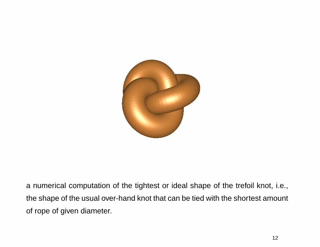
a numerical computation of the tightest or ideal shape of the trefoil knot, i.e.,

the shape of the usual over-hand knot that can be tied with the shortest amount

of rope of given diameter.

12

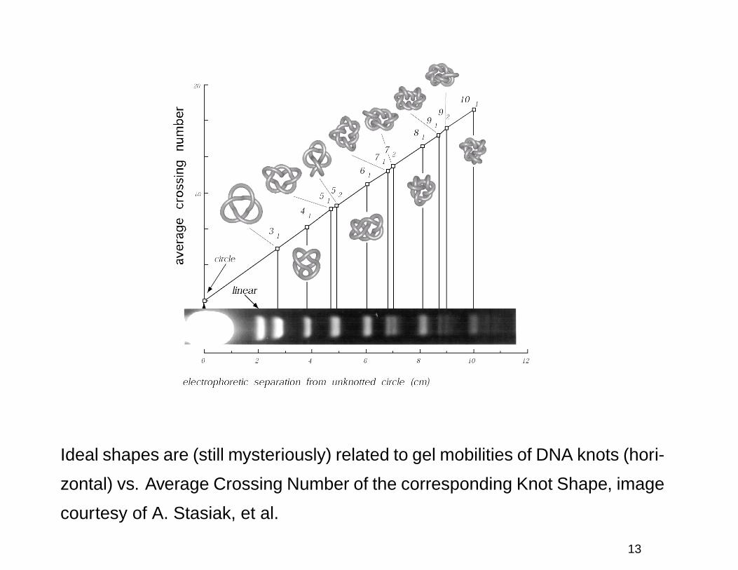
Ideal shapes are (still mysteriously) related to gel mobilities of DNA knots (hori-

zontal) vs. Average Crossing Number of the corresponding Knot Shape, image

courtesy of A. Stasiak, et al.

13

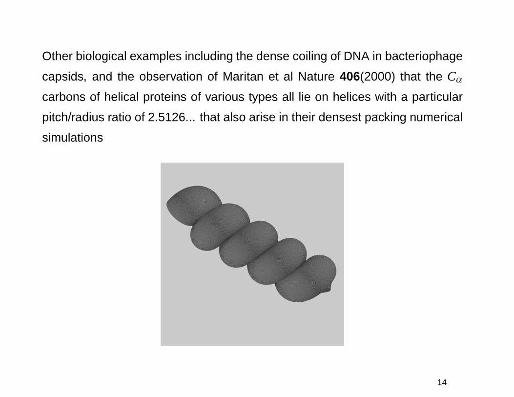
Other biological examples including the dense coiling of DNA in bacteriophage

capsids, and the observation of Maritan et al Nature 406(2000) that the Cα

carbons of helical proteins of various types all lie on helices with a particular

pitch/radius ratio of 2.5126... that also arise in their densest packing numerical

simulations

14

Plan of Lecture 1

Global radii of curvature, thickness and normal injectivity radius

· Self-distance of a curve, what is the big deal?

· Normal Injectivity Radius

· Global radii of curvature

· The case of Helices and optimal packings

· How the global radius of curvature is achieved

· The case of ellipses

15

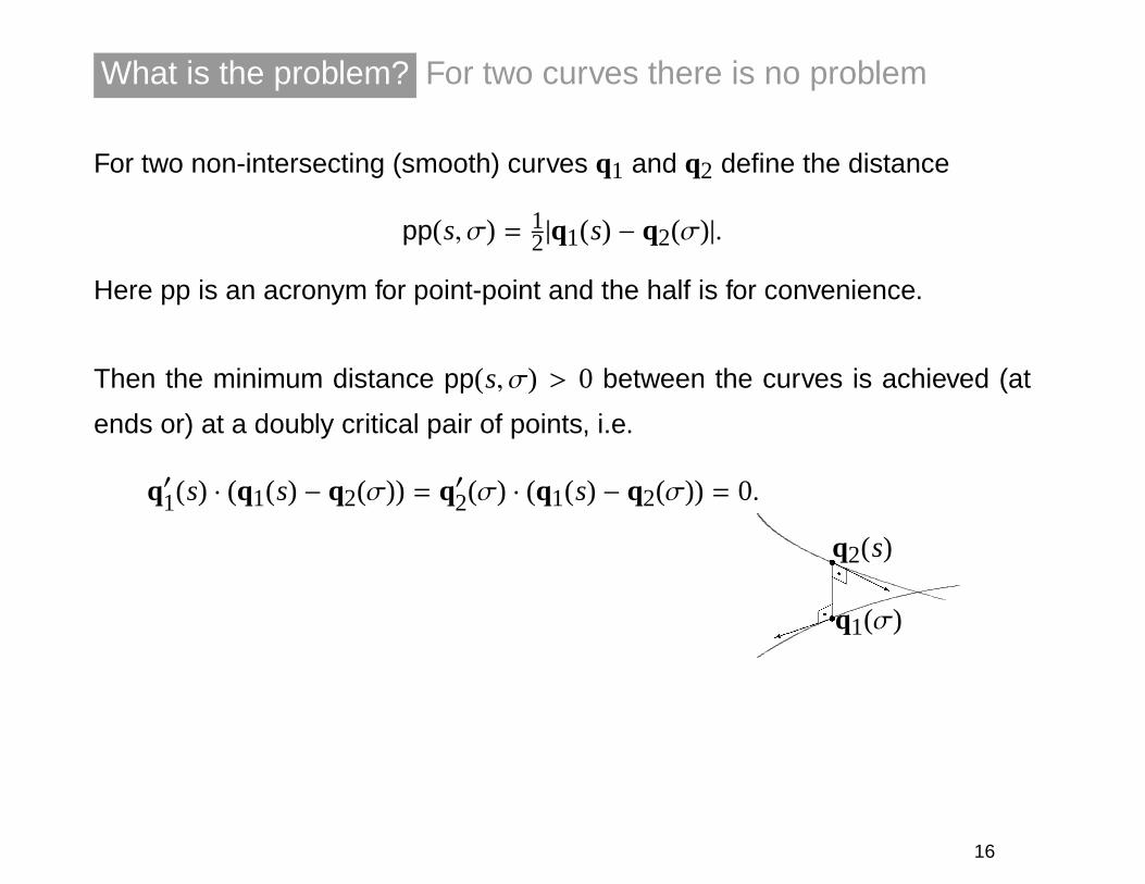
What is the problem? For two curves there is no problem

For two non-intersecting (smooth) curves q1 and q2 define the distance

pp(s, σ) = 12|q1(s) − q2(σ)|.

Here pp is an acronym for point-point and the half is for convenience.

Then the minimum distance pp(s, σ) > 0 between the curves is achieved (at

ends or) at a doubly critical pair of points, i.e.

q′1(s) · (q1(s) − q2(σ)) = q′2(σ) · (q1(s) − q2(σ)) = 0.

sq1(σ)

sq2(s)

�q����)

HqHHHHj

16

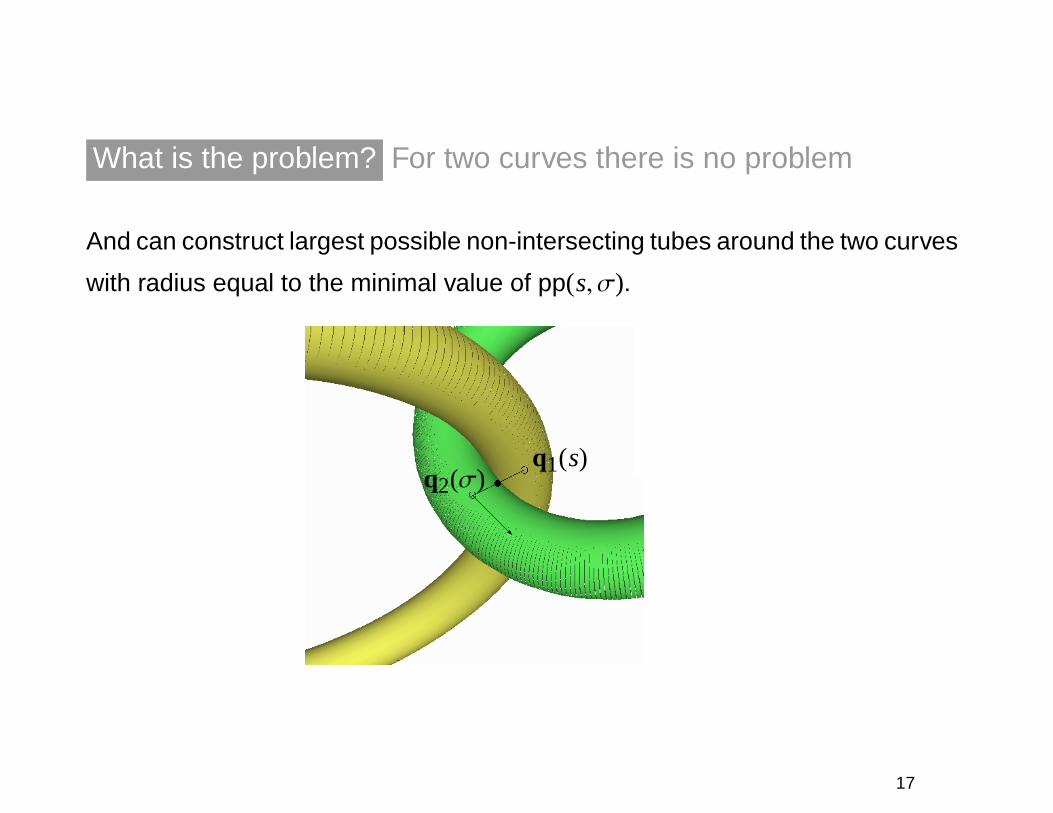
What is the problem? For two curves there is no problem

And can construct largest possible non-intersecting tubes around the two curves

with radius equal to the minimal value of pp(s, σ).

ddt ����q1(s)

q2(σ)@@@R

17

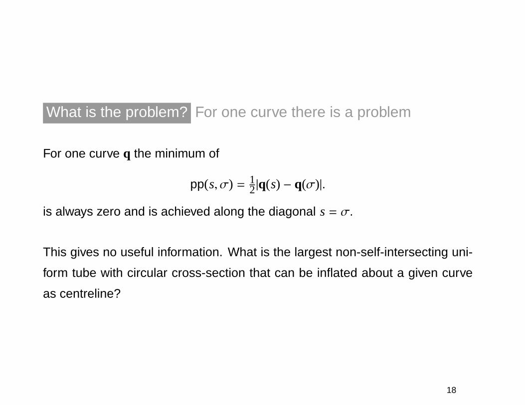
What is the problem? For one curve there is a problem

For one curve q the minimum of

pp(s, σ) = 12|q(s) − q(σ)|.

is always zero and is achieved along the diagonal s= σ.

This gives no useful information. What is the largest non-self-intersecting uni-

form tube with circular cross-section that can be inflated about a given curve

as centreline?

18

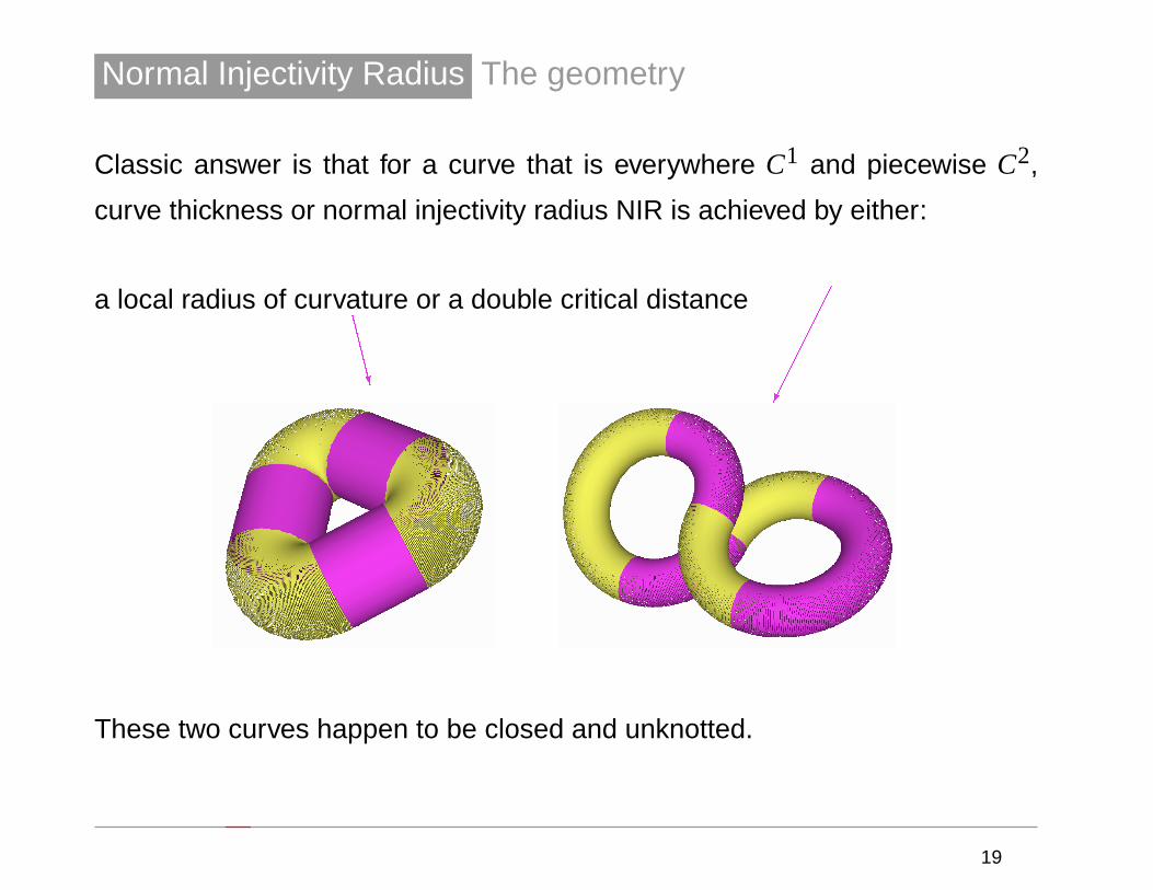
Normal Injectivity Radius The geometry

Classic answer is that for a curve that is everywhere C1 and piecewise C2,

curve thickness or normal injectivity radius NIR is achieved by either:

a local radius of curvature or a double critical distanceCCCCCW

���������

These two curves happen to be closed and unknotted.

19

Different notions of the thickness of a curve Curvature and DC set

NIR can be computed various ways, e.g., thickness ∆[q] of a (simple, closed)

curve q ∈ C2(S1,R3) is given by

∆[q] = min

{min

sρ(s),

12

min(s,σ)∈dc

|q(s) − q(σ)|

}where ρ(s) denotes the classic radius of curvature and dc is given by

dc= {(s, σ); q′(s) · (q(s) − q(σ)) = 0,q′(σ) · (q(s) − q(σ)) = 0, s, σ}

More explicit and useful than the geometric notion of NIR, but C2 is many ways

too strong a hypothesis, and the two alternatives are still a little cumbersome.

20

Different notions of the thickness of a curve

Global radius of curvature

The thickness ∆g[q] of a (simple, closed) curve q ∈ C0,1(S1,R3) is given by

∆g[q] = infs,σ,τ,s

r(q(s),q(σ),q(τ))

where r(x, y, z) denotes the radius of the circle through the points x, y, z.

Also for a given curve q introduce ppp(s, σ, τ) := r(q(s),q(σ),q(τ)). In other

words we interpret the radius ppp as a ‘distance’ between three points.

21

Different notions of the thickness of a curve

Global radius of curvature bounds and regularity

The functional ∆g[q] is well-defined for arc-length parameterised, closed C0,1-

curves. Such curves having an additional lower bound on thickness ∆g[q] ≥

θ > 0, are in fact differentiable and the tangent curve is Lipschitz continuous

with Lipschitz constant Kq′ ≤ θ−1. In other words, closed, arc-length parame-

terised, Lipschitz continuous curves with positive thickness, are actually C1,1-

curves, and therefore their curvature exists almost everywhere.

The bound ∆g[q] ≥ θ > 0 is weakly closed in W1,p for p > 1 which can be

exploited in the direct methods of the calculus of variations to prove existence

of C1,1-minimizers of various energy functionals.

C1,1 really seems to be the ‘natural’ smoothness of fattened curves.

22

Different notions of the thickness of a curve

Global and local radii of curvature and the DC set

The minimum of ∆g[q] is never achieved only at distinct points. For C2 curves

it is achieved either by a DC pair or by a classic osculating circle.

Proof is elementary geometry. Take the minimizing circle. Construct the asso-

ciated circumsphere with the given circle as a great-circle. If for example the

curve q enters the interior of this minimal circumsphere a contradiction arises

by shrinking the sphere and maintaining three intersections with the curve.

23

Global Radius of Curvature Functions

A global radius of curvature function along a curve q can be defined via min-

imisation over all but one argument

ρg(s) ≡ ρppp(s) := infσ,τ

r(q(s),q(σ),q(τ)) ≡ infσ,τ

ppp(s, σ, τ).

The (original) notation ρg(s) was introduced to emphasise that for C2 curves

q the classic local osculating circle is a competitor in the minimisation, so that

the global radius of curvature ρg(s) is a non-local generalisation of the limit of

the radius of the circle through three points all coalescent at s to the smallest

radius of all circles intersecting the curve three times.

The second notation ρppp(s) emphasises that the function is defined as an

infimum over the radius of a circle through three distinct points.

24

Global radii of curvature: Coalescence

As a matter of definition

∆g[q] = ∆ppp[q] = infsρppp(s) = inf

s,σ,τ,sr(q(s),q(σ),q(τ)) = inf

s,σ,τ,sppp(s, σ, τ)

where the equivalent notations emphasise different points of view.

In point of fact for C1,1 curves ρppp(s) is never realised only at three distinct

points, so that

ρppp(s) = infs,σ

pt(s, σ) =: ρpt(s)

The proof again involves the circumsphere to argue that the curve cannot

pierce the circumsphere of the circle realising the infimum.

For computation this simplification is significant.

25

Global radii of curvature: Pandora’s Box

With this point of view, starts to make sense to consider all circular and spher-

ical radii through respectively three and four points along a given curve, coa-

lescent or not in various combinations.

Lots of combinations all of which give rise to a global radius of curvature func-

tion.

Note: the different functions require slightly different regularities. But for all the

functions a pair of doubly critical points is very special.

26

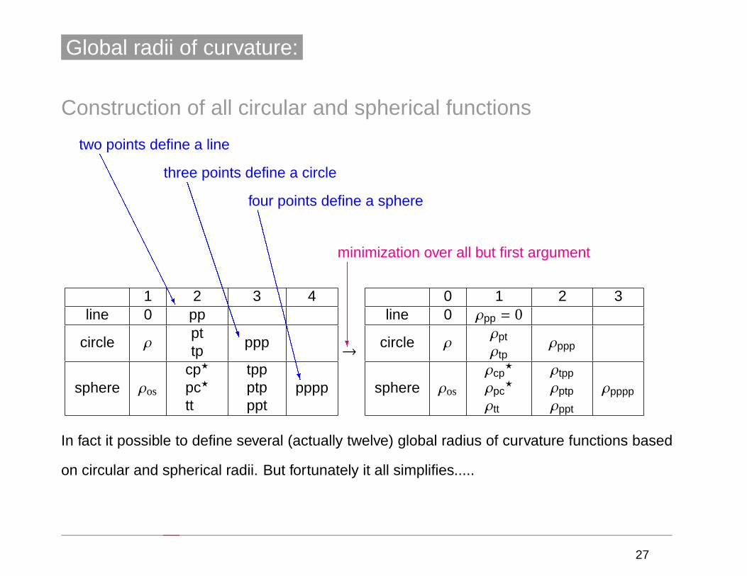
Global radii of curvature:

Construction of all circular and spherical functions

1 2 3 4line 0 pp

circle ρpttp

ppp

sphere ρos

cp?

pc?

tt

tppptpppt

pppp

→

minimization over all but first argument

two points define a line

three points define a circle

four points define a sphere

?

AAAAAAAAAAAAAAAAU

BBBBBBBBBBBBBBBBBN

CCCCCCCCCCCCCCCCCCW

0 1 2 3line 0 ρpp = 0

circle ρρpt

ρtpρppp

sphere ρos

ρcp?

ρpc?

ρtt

ρtpp

ρptp

ρppt

ρpppp

In fact it possible to define several (actually twelve) global radius of curvature functions based

on circular and spherical radii. But fortunately it all simplifies.....

27

Global radii of curvature: Not so many cases important

Proposition: Under certain hypotheses:

ρos≥

{ρ = ρ?cp ≥ ρtp = ρtt = ρtpp

ρpc

}≥ ρpt = ρppp = ρptp = ρppt = ρpppp ≥ 0,

and all inequalities are sharp for some curves.

When minimal regularity is of concern consider the functions ppp and pppp and their associ-ated global curvatures ρppp and ρpppp.

Otherwise concentrate on the classic local curvatures ρ and ρos, and the circular functionpt(s, σ) and the two global curvatures it generates namely ρpt and ρtp via minimization overrespectively its second and first arguments.

→ For computations the useful global radius of curvature functions that characteriseNIR are ρpt and ρtp.

Lemma: Under certain hypotheses:

∆[q] = ∆pt[q] := infsρpt(s),

= ∆tp[q] := infsρtp(s).

28

Global radii of curvature: The example of helices

(Circular) Helices are uniform so any curvature function will be constant, and

any two argument radius function will depend only on the difference (s−σ) =: η

of the two arc-length arguments.

By dilation can scale so that the radius of the cylinder is 1, and then only

remaining free parameter is the pitch.

Helices map back to themselves when rotated through π about a principal nor-

mal, and this symmetry implies pt(s, σ) = pt(σ, s).

29

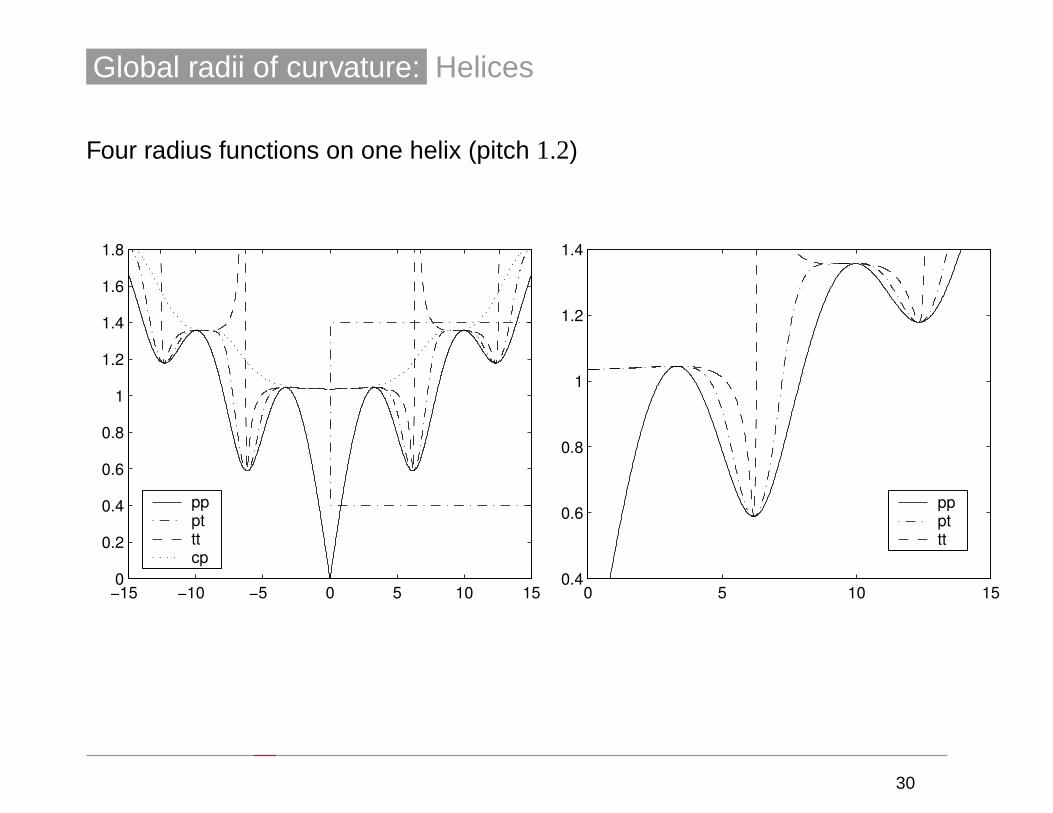
Global radii of curvature: Helices

Four radius functions on one helix (pitch 1.2)

−15 −10 −5 0 5 10 150

0.2

0.4

0.6

0.8

1

1.2

1.4

1.6

1.8

ppptttcp

0 5 10 150.4

0.6

0.8

1

1.2

1.4

pppttt

30

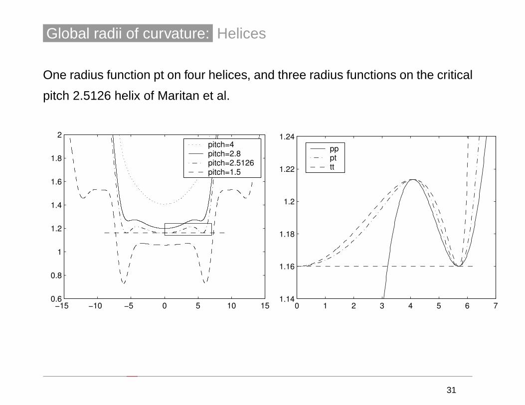
Global radii of curvature: Helices

One radius function pt on four helices, and three radius functions on the critical

pitch 2.5126 helix of Maritan et al.

−15 −10 −5 0 5 10 150.6

0.8

1

1.2

1.4

1.6

1.8

2pitch=4 pitch=2.8 pitch=2.5126pitch=1.5

0 1 2 3 4 5 6 71.14

1.16

1.18

1.2

1.22

1.24pppttt

31

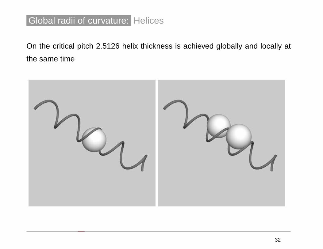
Global radii of curvature: Helices

On the critical pitch 2.5126 helix thickness is achieved globally and locally at

the same time

32

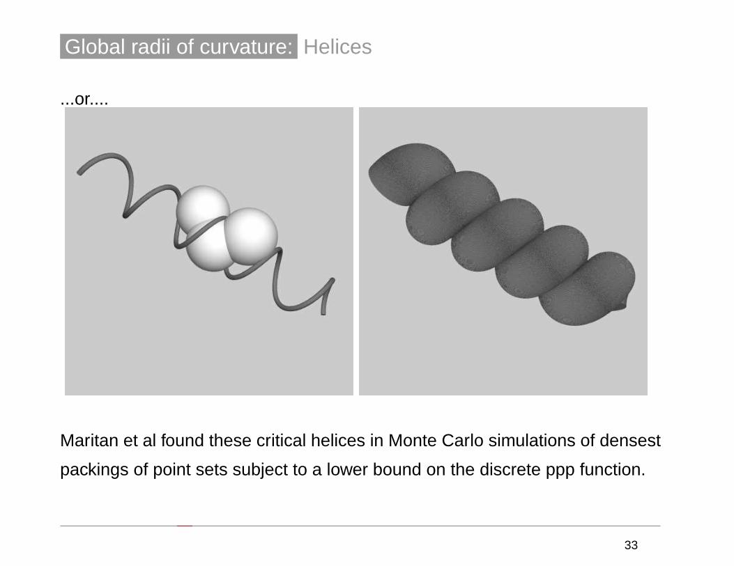
Global radii of curvature: Helices

...or....

Maritan et al found these critical helices in Monte Carlo simulations of densest

packings of point sets subject to a lower bound on the discrete ppp function.

33

Plan of Lecture 1

Global radii of curvature, thickness and normal injectivity radius

· Self-distance of a curve, what is the big deal?

· Normal Injectivity Radius

· Global radii of curvature

· The case of Helices and optimal packings

· How the global radius of curvature is achieved

· The case of ellipses

34

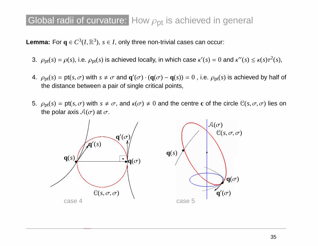
Global radii of curvature: How ρpt is achieved in general

Lemma: For q ∈ C3(I ,R3), s ∈ I , only three non-trivial cases can occur:

3. ρpt(s) = ρ(s), i.e. ρpt(s) is achieved locally, in which case κ′(s) = 0 and κ′′(s) ≤ κ(s)τ2(s),

4. ρpt(s) = pt(s, σ) with s, σ and q′(σ) · (q(σ) − q(s)) = 0 , i.e. ρpt(s) is achieved by half ofthe distance between a pair of single critical points,

5. ρpt(s) = pt(s, σ) with s , σ, and κ(σ) , 0 and the centre c of the circle C(s, σ, σ) lies onthe polar axis A(σ) at σ.

tq(s)

q′(s)

trq(σ)

q′(σ)

C(s, σ, σ)case 4

tq(s)

t�

�

q(σ)

q′(σ)

C(s, σ, σ)A(σ)

case 5

35

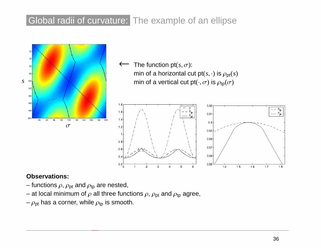
Global radii of curvature: The example of an ellipse

s

σ

← The function pt(s, σ):min of a horizontal cut pt(s, ·) is ρpt(s)min of a vertical cut pt(·, σ) is ρtp(σ)

Observations:– functions ρ, ρpt and ρtp are nested,– at local minimum of ρ all three functions ρ, ρpt and ρtp agree,– ρpt has a corner, while ρtp is smooth.

36

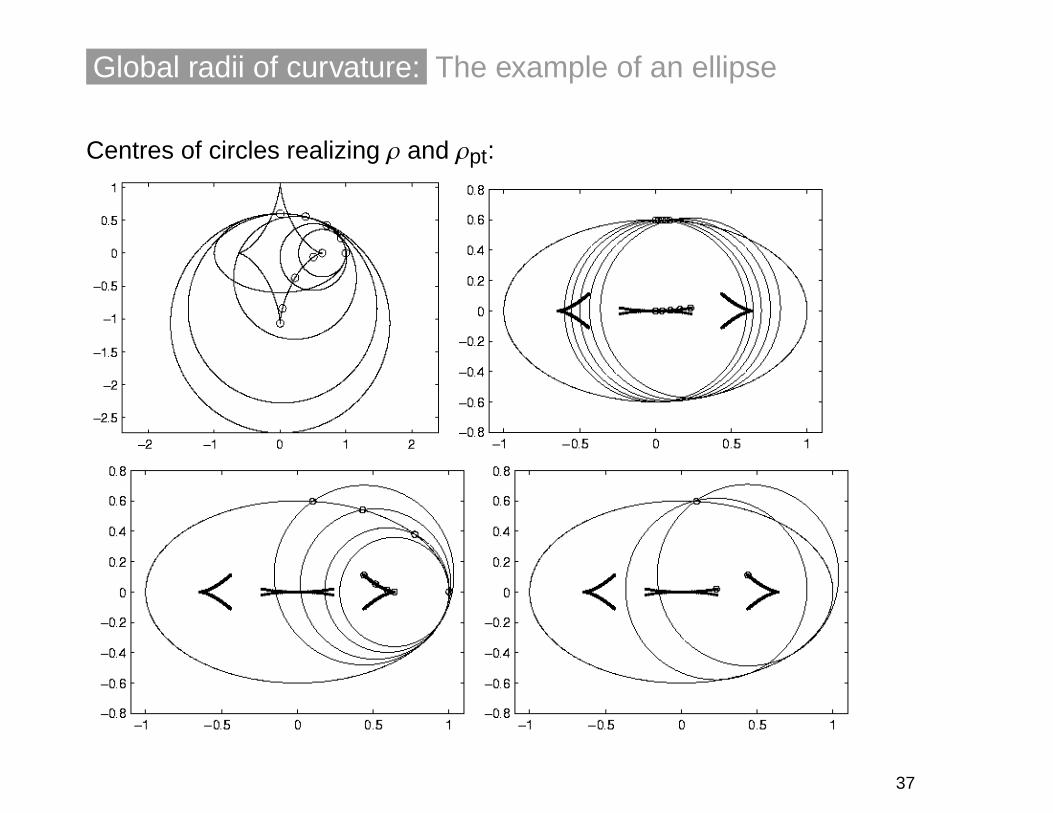
Global radii of curvature: The example of an ellipse

Centres of circles realizing ρ and ρpt:

37

Lecture 2

The Biarc discretisation of space curves. How to compute interesting curves

with accurate evaluation of global radii of curvature and thickness

38

Plan of Lecture 2:

· biarcs: construction and convergence results

· evaluation of thickness and ρpt on arc curves

· biarc approximation of an ellipse and its global radius of curvature functions

· stop early, eat, drink, be merry...

39

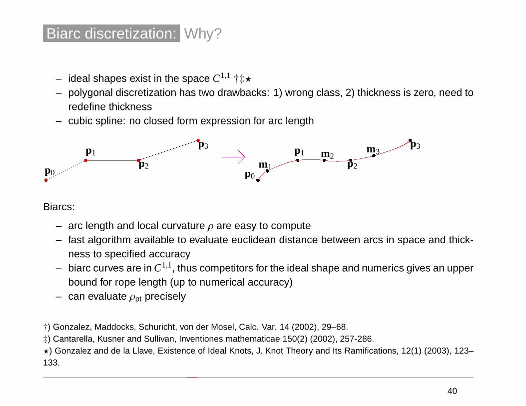
Biarc discretization: Why?

– ideal shapes exist in the space C1,1 †‡?

– polygonal discretization has two drawbacks: 1) wrong class, 2) thickness is zero, need toredefine thickness

– cubic spline: no closed form expression for arc length

t

t t

t

p0

p1

p2

p3

����

�����

������

@�

t

t t

t

p0

p1

p2

p3

tt t

m1

m2m3

Biarcs:

– arc length and local curvature ρ are easy to compute– fast algorithm available to evaluate euclidean distance between arcs in space and thick-

ness to specified accuracy– biarc curves are in C1,1, thus competitors for the ideal shape and numerics gives an upper

bound for rope length (up to numerical accuracy)– can evaluate ρpt precisely

†) Gonzalez, Maddocks, Schuricht, von der Mosel, Calc. Var. 14 (2002), 29–68.‡) Cantarella, Kusner and Sullivan, Inventiones mathematicae 150(2) (2002), 257-286.?) Gonzalez and de la Llave, Existence of Ideal Knots, J. Knot Theory and Its Ramifications, 12(1) (2003), 123–133.

40

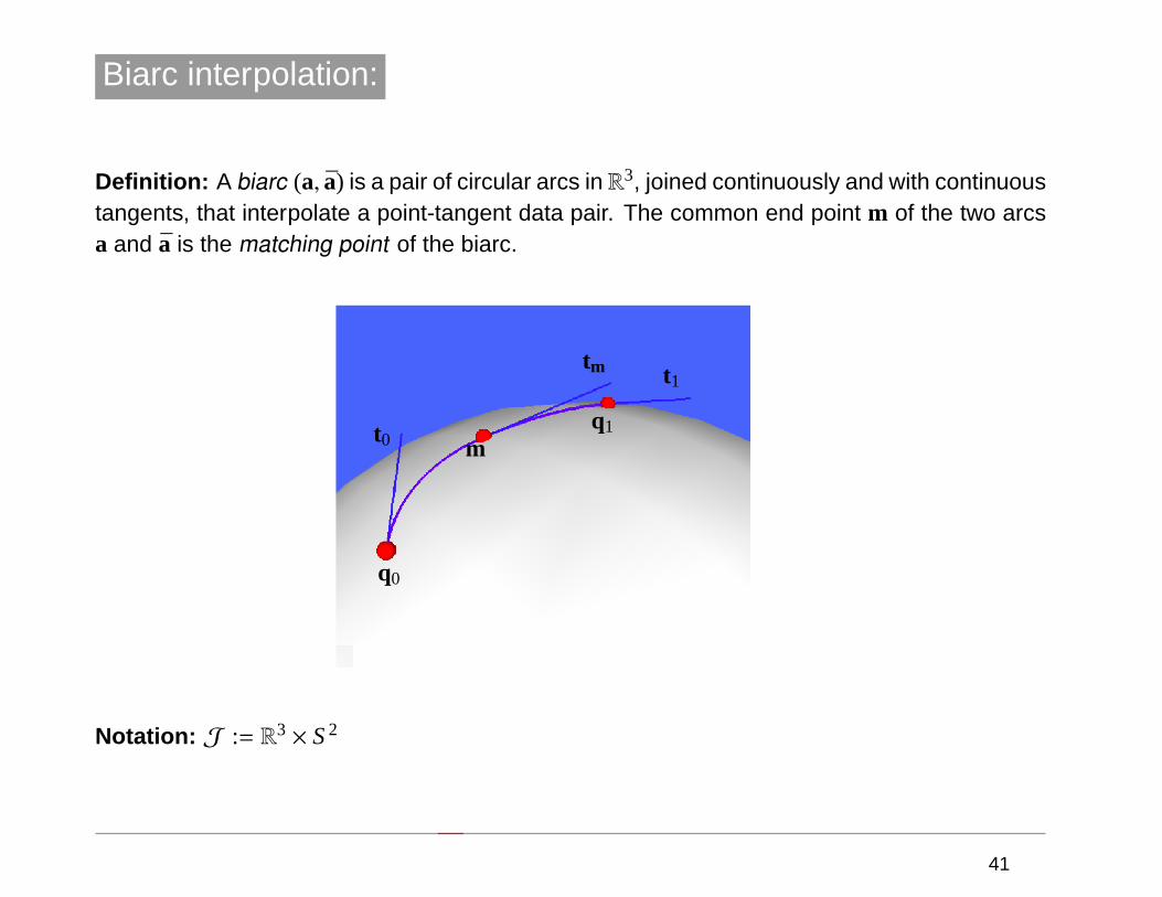
Biarc interpolation:

Definition: A biarc (a, a) is a pair of circular arcs in R3, joined continuously and with continuoustangents, that interpolate a point-tangent data pair. The common end point m of the two arcsa and a is the matching point of the biarc.

q0

q1t0

t1

m

tm

Notation: J := R3 × S2

41

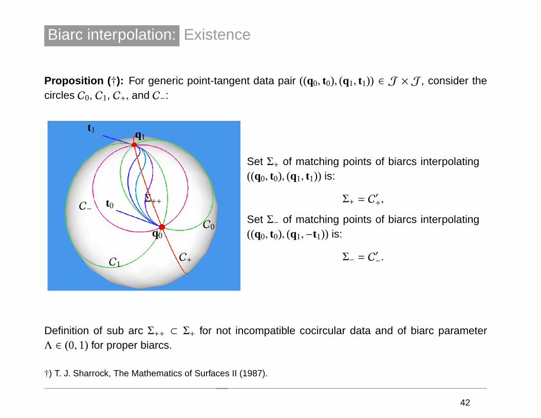
Biarc interpolation: Existence

Proposition ( †): For generic point-tangent data pair ((q0, t0), (q1, t1)) ∈ J × J , consider thecircles C0, C1, C+, and C−:

q0

q1

t0

t1

C0

C1C+

C−Σ++

Set Σ+ of matching points of biarcs interpolating((q0, t0), (q1, t1)) is:

Σ+ = C′+,

Set Σ− of matching points of biarcs interpolating((q0, t0), (q1,−t1)) is:

Σ− = C′−.

Definition of sub arc Σ++ ⊂ Σ+ for not incompatible cocircular data and of biarc parameterΛ ∈ (0,1) for proper biarcs.

†) T. J. Sharrock, The Mathematics of Surfaces II (1987).

42

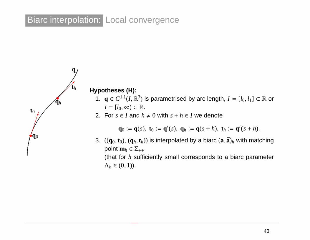
Biarc interpolation: Local convergence

u

u

q0

qh

��������

������

t0

th

q

Hypotheses (H):1. q ∈ C1,1(I ,R3) is parametrised by arc length, I = [l0, l1] ⊂ R or

I = [l0,∞) ⊂ R.2. For s ∈ I and h , 0 with s+ h ∈ I we denote

q0 := q(s), t0 := q′(s), qh := q(s+ h), th := q′(s+ h).

3. ((q0, t0), (qh, th)) is interpolated by a biarc (a, a)h with matchingpoint mh ∈ Σ++

(that for h sufficiently small corresponds to a biarc parameterΛh ∈ (0,1)).

43

Biarc interpolation: Local convergence

Proposition:

hypotheses: expansions:

(H) λ((a, a)h) − h = O(h3)

(H), q ∈ C2, 0 < Λmin ≤ Λh |q′′(s) − a′′h+| = o(1)

�

constant depends only on Kq′

�

arc a of biarc (a, a)h approaches the osculating circle at q0

speed of convergence independent of s if q′′ uniformly continuous

44

Biarc interpolation: Global convergence

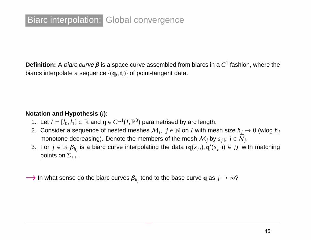
Definition: A biarc curve β is a space curve assembled from biarcs in a C1 fashion, where thebiarcs interpolate a sequence {(qi, t i)} of point-tangent data.

Notation and Hypothesis ( i):1. Let I = [l0, l1] ⊂ R and q ∈ C1,1(I ,R3) parametrised by arc length.2. Consider a sequence of nested meshesM j, j ∈ N on I with mesh size h j → 0 (wlog h j

monotone decreasing). Denote the members of the meshM j by sj,i, i ∈ N j.3. For j ∈ N βhj

is a biarc curve interpolating the data (q(sj,i),q′(sj,i)) ∈ J with matchingpoints on Σ++.

→ In what sense do the biarc curves βhjtend to the base curve q as j → ∞?

45

Biarc interpolation: Global convergence of arc length

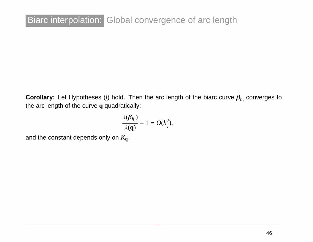
Corollary: Let Hypotheses (i) hold. Then the arc length of the biarc curve βhjconverges to

the arc length of the curve q quadratically:

λ(βhj)

λ(q)− 1 = O(h2

j ),

and the constant depends only on Kq′.

46

Biarc interpolation: Global convergence

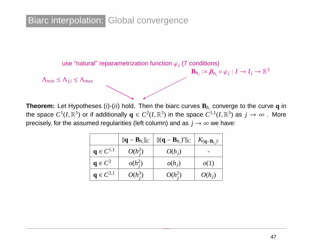
use “natural” reparametrization function ϕ j (7 conditions)Bhj

:= βhj◦ ϕ j : I → I j → R

3

Λmin ≤ Λ j,i ≤ ΛmaxHHHHHHHj

������������

Theorem: Let Hypotheses (i)-(ii ) hold. Then the biarc curves Bhjconverge to the curve q in

the space C1(I ,R3) or if additionally q ∈ C2(I ,R3) in the space C1,1(I ,R3) as j → ∞ . Moreprecisely, for the assumed regularities (left column) and as j → ∞ we have:

‖q − Bhj‖C ‖(q − Bhj

)′‖C K(q−Bhj)′

q ∈ C1,1 O(h2j ) O(h j) -

q ∈ C2 o(h2j ) o(h j) o(1)

q ∈ C2,1 O(h3j ) O(h2

j ) O(h j)

47

Plan of Lecture 2:

· biarcs: construction and convergence results

· evaluation of thickness and ρpt on arc curves

· biarc approximation of an ellipse and its global radius of curvature functions

· stop early, eat, drink, be merry...

48

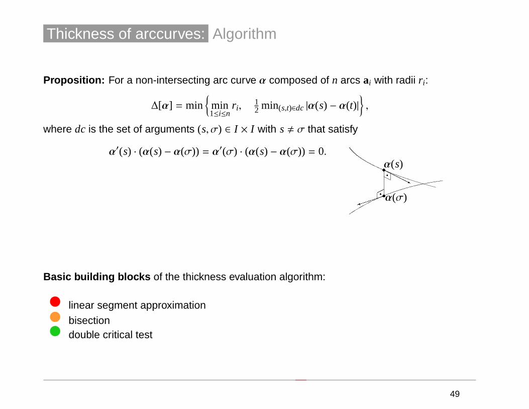
Thickness of arccurves: Algorithm

Proposition: For a non-intersecting arc curve α composed of n arcs ai with radii r i:

∆[α] = min{

min1≤i≤n

r i,12 min(s,t)∈dc |α(s) − α(t)|

},

where dc is the set of arguments (s, σ) ∈ I × I with s, σ that satisfy

α′(s) · (α(s) − α(σ)) = α′(σ) · (α(s) − α(σ)) = 0.

sα(σ)

sα(s)

�q����)

HqHHHHj

Basic building blocks of the thickness evaluation algorithm:

• linear segment approximation

• bisection• double critical test

49

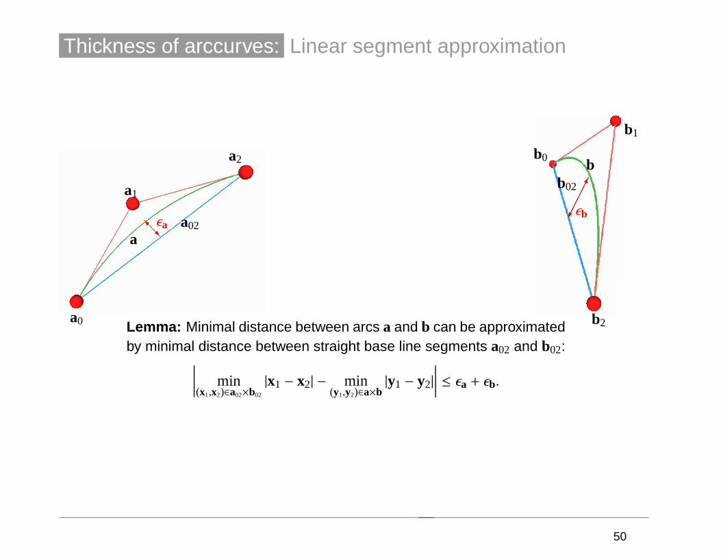
Thickness of arccurves: Linear segment approximation

aa02

a0

a1

a2

@@I@@Rεa

bb02

b0

b1

b2

��������

���� εb

Lemma: Minimal distance between arcs a and b can be approximatedby minimal distance between straight base line segments a02 and b02:∣∣∣∣∣ min

(x1,x2)∈a02×b02

|x1 − x2| − min(y1,y2)∈a×b

|y1 − y2|

∣∣∣∣∣ ≤ εa + εb.

50

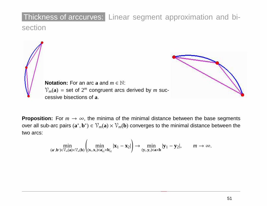
Thickness of arccurves: Linear segment approximation and bi-section

Notation: For an arc a and m ∈ N:Vm(a) = set of 2m congruent arcs derived by m suc-cessive bisections of a.

Proposition: For m → ∞, the minima of the minimal distance between the base segmentsover all sub-arc pairs (a∗,b∗) ∈ Vm(a) × Vm(b) converges to the minimal distance between thetwo arcs:

min(a∗,b∗)∈Vm(a)×Vm(b)

(min

(x1,x2)∈a∗02×b∗02

|x1 − x2|

)→ min

(y1,y2)∈a×b|y1 − y2|, m→ ∞.

51

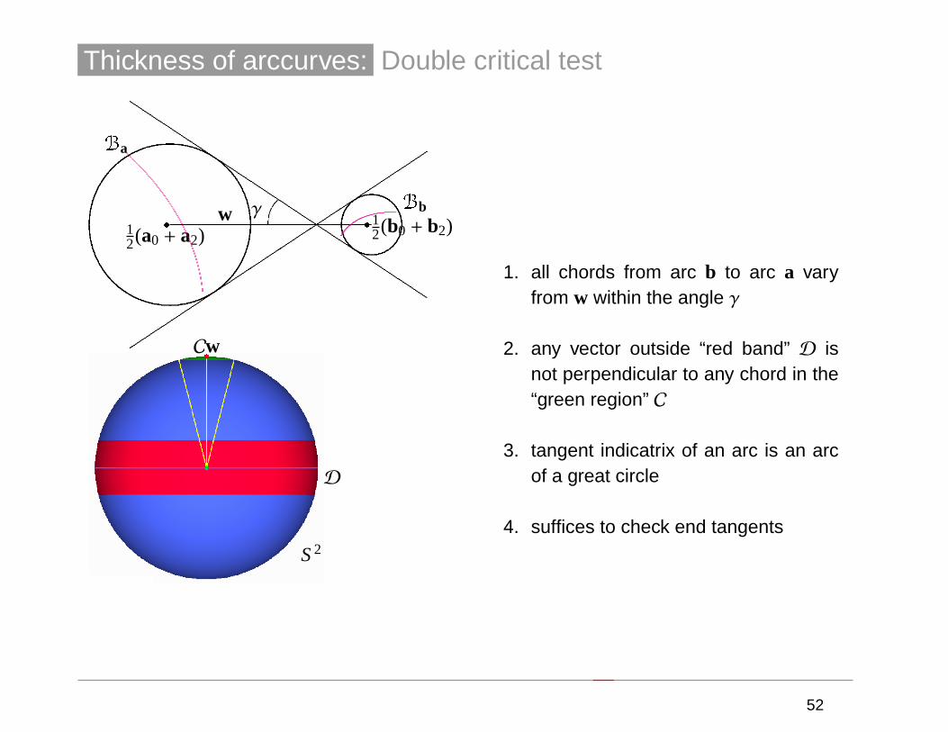
Thickness of arccurves: Double critical test

Ba

Bbγws s12(a0 + a2)

12(b0 + b2)

w

D

S2

C

1. all chords from arc b to arc a varyfrom w within the angle γ

2. any vector outside “red band” D isnot perpendicular to any chord in the“green region” C

3. tangent indicatrix of an arc is an arcof a great circle

4. suffices to check end tangents

52

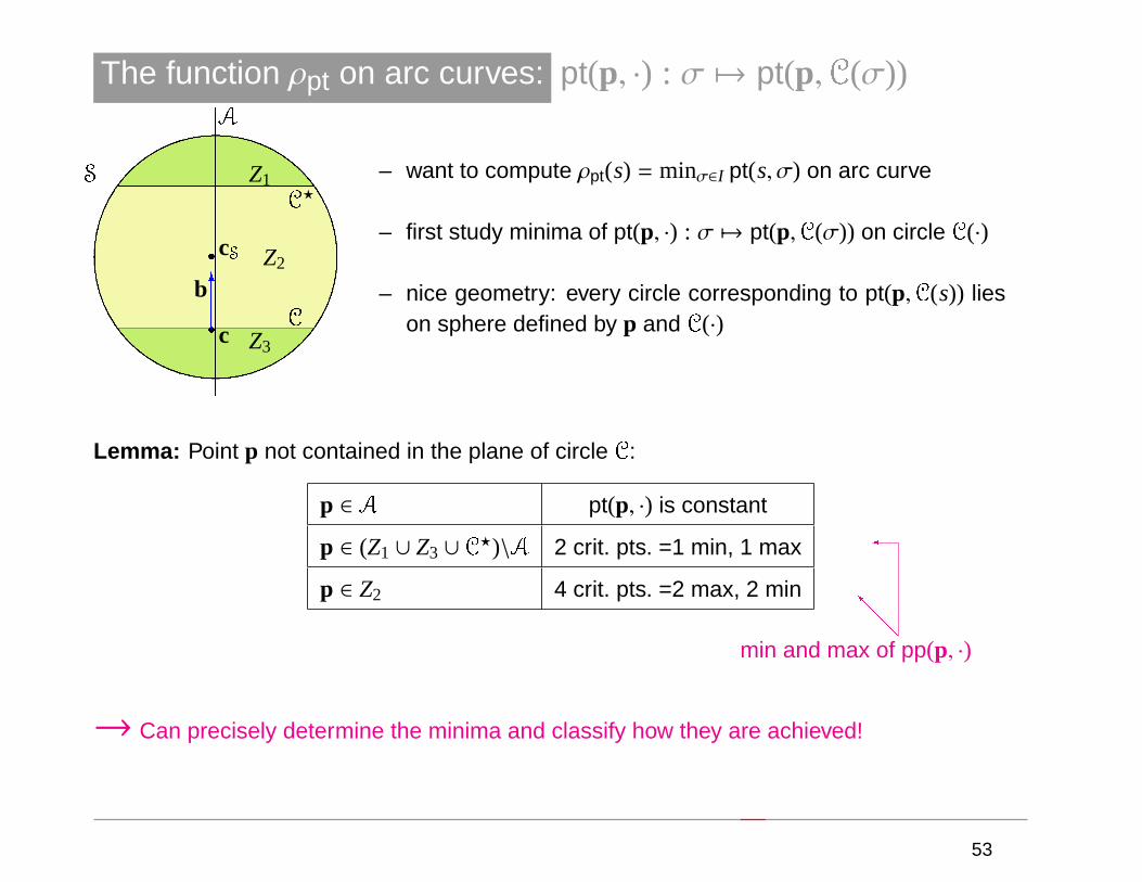
The function ρpt on arc curves: pt(p, ·) : σ 7→ pt(p,C(σ))A

S

C

C?

sc

scS

Z1

Z2

Z3

6b

– want to compute ρpt(s) = minσ∈I pt(s, σ) on arc curve

– first study minima of pt(p, ·) : σ 7→ pt(p,C(σ)) on circle C(·)

– nice geometry: every circle corresponding to pt(p,C(s)) lieson sphere defined by p and C(·)

Lemma: Point p not contained in the plane of circle C:

p ∈ A pt(p, ·) is constant

p ∈ (Z1 ∪ Z3 ∪ C?)\A 2 crit. pts. =1 min, 1 max

p ∈ Z2 4 crit. pts. =2 max, 2 min

min and max of pp(p, ·)@

@@I

�

→ Can precisely determine the minima and classify how they are achieved!

53

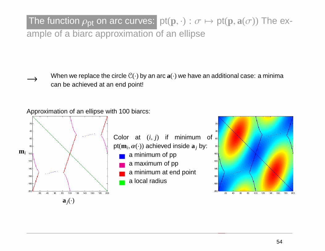
The function ρpt on arc curves: pt(p, ·) : σ 7→ pt(p,a(σ)) The ex-ample of a biarc approximation of an ellipse

→ When we replace the circle C(·) by an arc a(·) we have an additional case: a minimacan be achieved at an end point!

Approximation of an ellipse with 100 biarcs:

mi

a j(·)

Color at (i, j) if minimum ofpt(mi,α(·)) achieved inside a j by:

. a minimum of pp

. a maximum of pp

. a minimum at end point

. a local radius

54

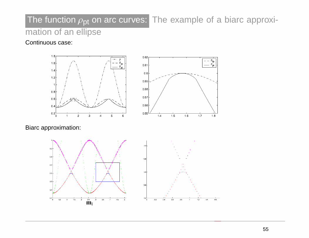
The function ρpt on arc curves: The example of a biarc approxi-mation of an ellipseContinuous case:

Biarc approximation:

mi

55

Plan of Lecture 2:

· biarcs: construction and convergence results

· evaluation of thickness and ρpt on arc curves

· biarc approximation of an ellipse and its global radius of curvature functions

· stop early, eat, drink, be merry...

56

Plan of Lecture 3: Computations of Ideal Shapes

· introduction: knots and ideal shapes of knots

· definition of contact and approximate µ-contact sets

· computations of the ideal 3.1-knot

· computations of the ideal 4.1-knot

· Conclusions

57

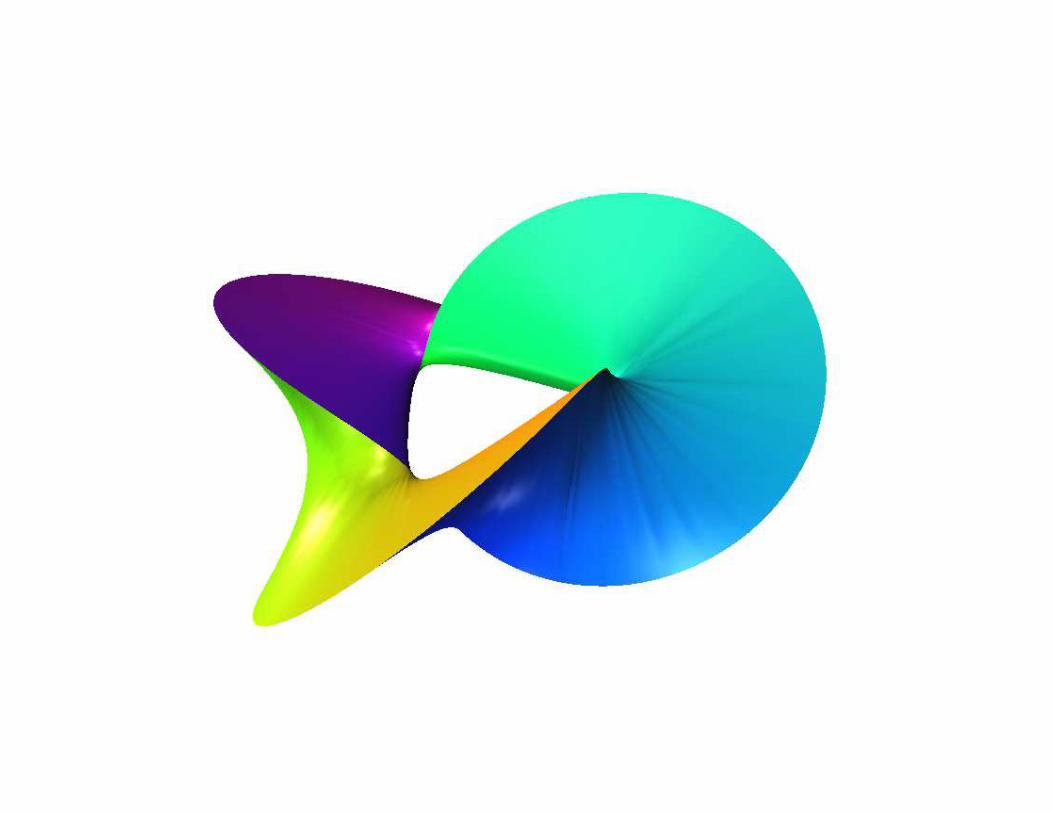
Our objective is to describe how this visualisation of a shaded triangulation of

the contact chords of the (approximately) ideal trefoil is computed:

58

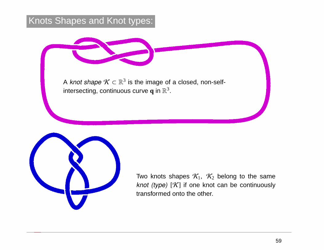
Knots Shapes and Knot types:

A knot shape K ⊂ R3 is the image of a closed, non-self-intersecting, continuous curve q in R3.

Two knots shapes K1, K2 belong to the sameknot (type) [K ] if one knot can be continuouslytransformed onto the other.

59

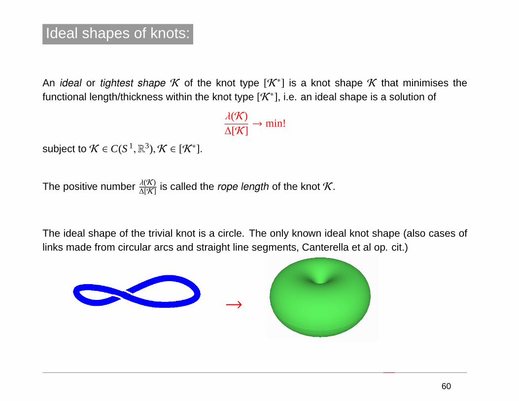
Ideal shapes of knots:

An ideal or tightest shape K of the knot type [K∗] is a knot shape K that minimises thefunctional length/thickness within the knot type [K∗], i.e. an ideal shape is a solution of

λ(K)∆[K ]

→ min!

subject to K ∈ C(S1,R3),K ∈ [K∗].

The positive number λ(K)∆[K ] is called the rope length of the knot K .

The ideal shape of the trivial knot is a circle. The only known ideal knot shape (also cases oflinks made from circular arcs and straight line segments, Canterella et al op. cit.)

→

60

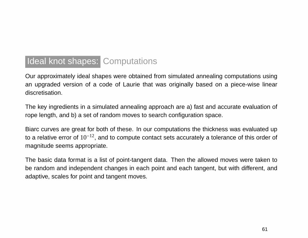
Ideal knot shapes: Computations

Our approximately ideal shapes were obtained from simulated annealing computations usingan upgraded version of a code of Laurie that was originally based on a piece-wise lineardiscretisation.

The key ingredients in a simulated annealing approach are a) fast and accurate evaluation ofrope length, and b) a set of random moves to search configuration space.

Biarc curves are great for both of these. In our computations the thickness was evaluated upto a relative error of 10−12, and to compute contact sets accurately a tolerance of this order ofmagnitude seems appropriate.

The basic data format is a list of point-tangent data. Then the allowed moves were taken tobe random and independent changes in each point and each tangent, but with different, andadaptive, scales for point and tangent moves.

61

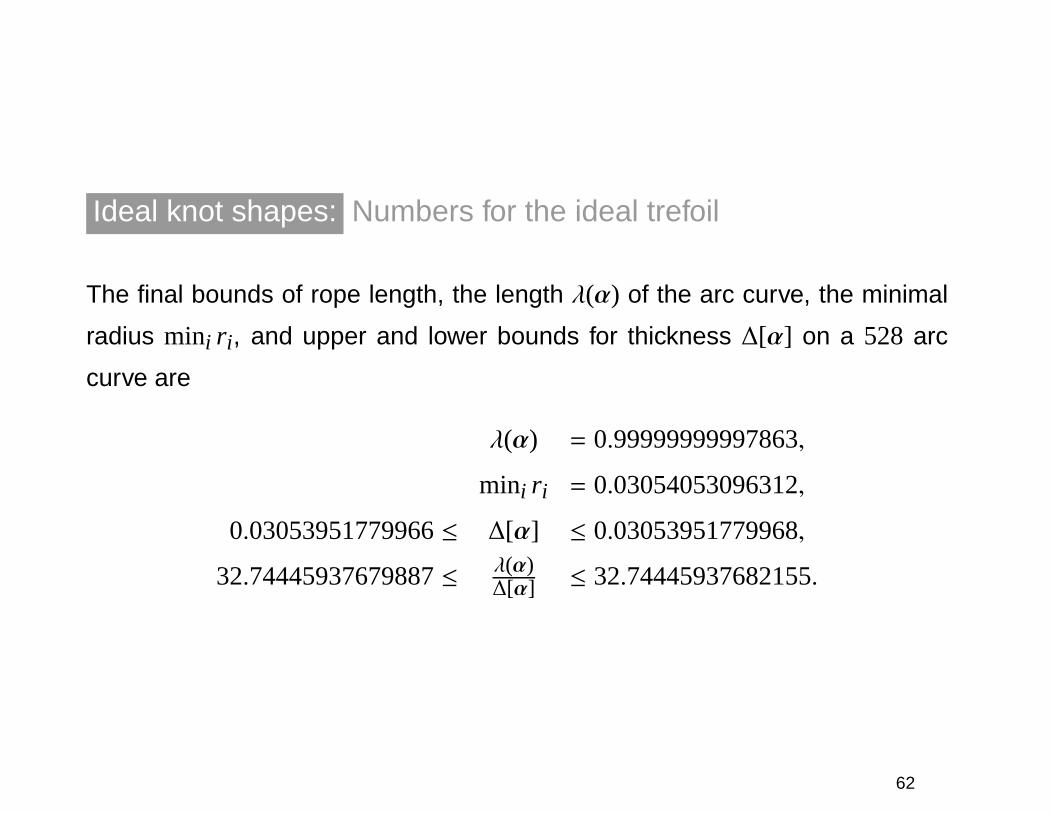
Ideal knot shapes: Numbers for the ideal trefoil

The final bounds of rope length, the length λ(α) of the arc curve, the minimal

radius mini r i, and upper and lower bounds for thickness ∆[α] on a 528 arc

curve are

λ(α) = 0.99999999997863,

mini r i = 0.03054053096312,

0.03053951779966≤ ∆[α] ≤ 0.03053951779968,

32.74445937679887≤ λ(α)∆[α] ≤ 32.74445937682155.

62

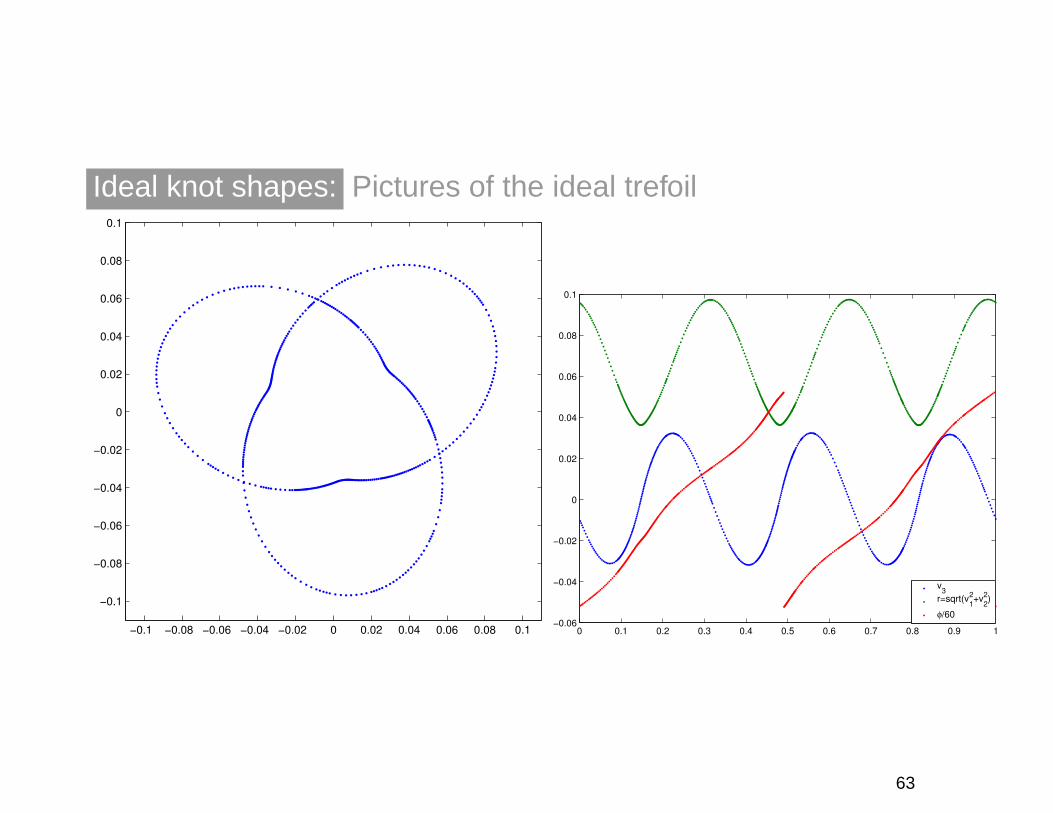
Ideal knot shapes: Pictures of the ideal trefoil

−0.1 −0.08 −0.06 −0.04 −0.02 0 0.02 0.04 0.06 0.08 0.1

−0.1

−0.08

−0.06

−0.04

−0.02

0

0.02

0.04

0.06

0.08

0.1

0 0.1 0.2 0.3 0.4 0.5 0.6 0.7 0.8 0.9 1−0.06

−0.04

−0.02

0

0.02

0.04

0.06

0.08

0.1

v3

r=sqrt(v12+v

22)

φ/60

63

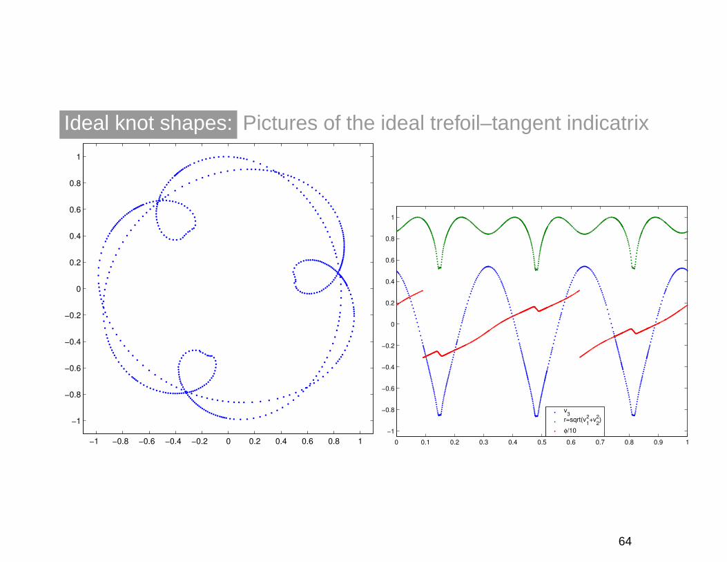
Ideal knot shapes: Pictures of the ideal trefoil–tangent indicatrix

−1 −0.8 −0.6 −0.4 −0.2 0 0.2 0.4 0.6 0.8 1

−1

−0.8

−0.6

−0.4

−0.2

0

0.2

0.4

0.6

0.8

1

0 0.1 0.2 0.3 0.4 0.5 0.6 0.7 0.8 0.9 1

−1

−0.8

−0.6

−0.4

−0.2

0

0.2

0.4

0.6

0.8

1

v3

r=sqrt(v12+v

22)

φ/10

64

Ideal knot shapes: Necessary conditions for ideality

Very little known about necessary conditions for ideality. On segments where

the curve is C2 have:

1) The segment is either straight or the function ρpt(s) is constant and minimal,

i.e., equal to the thickness ∆.

2) (A complicated version involving Radon measure of the idea) If local curva-

ture is not active anywhere, and at curved points of the shape, the principal

normal of the curve should be in the cone of contact chords, i.e., of doubly

critical line segments realising ∆. (vdMosel & Schuricht).

Therefore we need to understand the....

65

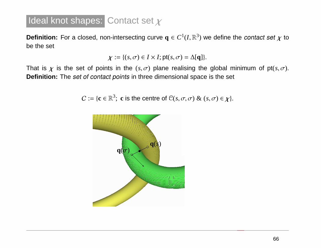
Ideal knot shapes: Contact set χ

Definition: For a closed, non-intersecting curve q ∈ C1(I ,R3) we define the contact set χ tobe the set

χ := {(s, σ) ∈ I × I ; pt(s, σ) = ∆[q]}.

That is χ is the set of points in the (s, σ) plane realising the global minimum of pt(s, σ).Definition: The set of contact points in three dimensional space is the set

C := {c ∈ R3; c is the centre of C(s, σ, σ) & ( s, σ) ∈ χ}.

ddt ����q(s)

q(σ)@@@R

66

Ideal knot shapes: Understanding Contact Sets

For a generic curve the global minimiser of pt will be realised at a single point

and both χ and C will be sets containing one point. Such sets are robust.

The ellipse has symmetry, so there are a two points in each set corresponding

to the two points of minimal radius of curvature. Already an unstable situation.

And for ideal shapes constancy of ρpt implies that the exact contact sets should

probably be much larger, i.e., at least contain line segments. A very unstable

situation under perturbation.

For example the point contact set C for the circle (i.e., the unknot ideal shape)

is a single point, namely the centre. But the contact set χ is the entire square

I × I , because pt is constant on circles.

67

Ideal knot shapes: Approximate contact set χµ

→ Thus for approximately ideal shapes, and in particular for numerics we

need to introduce a tolerance!

Definition: For each µ > 0 the µ-contact set χµ is the set

χµ := {(s, σ) ∈ I× I ; pt(s, σ) ≤ ∆[q](1+µ) & pt(s, ·) has a local minimum in σ},

and the set of µ-contact points in three dimensional space is the set

Cµ := {c ∈ R3; c is the centre of C(s, σ, σ) & ( s, σ) ∈ χµ}.

68

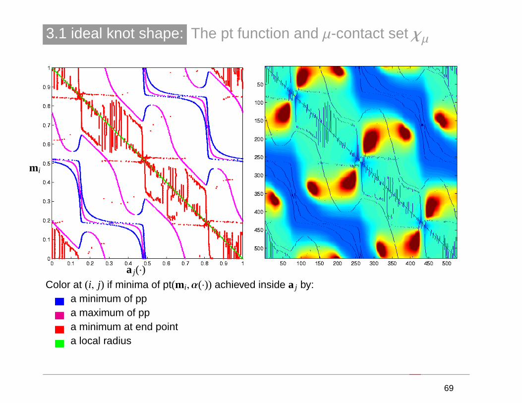
3.1 ideal knot shape: The pt function and µ-contact set χµ

mi

a j(·)Color at (i, j) if minima of pt(mi,α(·)) achieved inside a j by:

. a minimum of pp

. a maximum of pp

. a minimum at end point

. a local radius

69

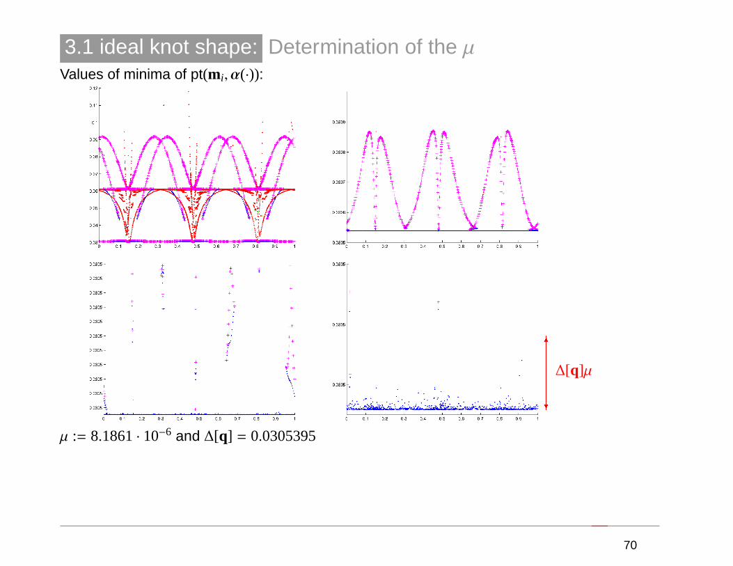
3.1 ideal knot shape: Determination of the µValues of minima of pt(mi,α(·)):

6

?

∆[q]µ

µ := 8.1861· 10−6 and ∆[q] = 0.0305395

70

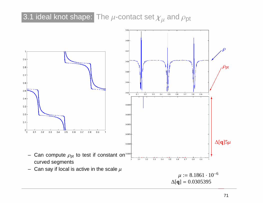
3.1 ideal knot shape: The µ-contact set χµ and ρpt

6

?

∆[q]5µ

µ := 8.1861· 10−6

∆[q] = 0.0305395

ρ

ρpt

��

�

��������

– Can compute ρpt to test if constant oncurved segments

– Can say if local is active in the scale µ

71

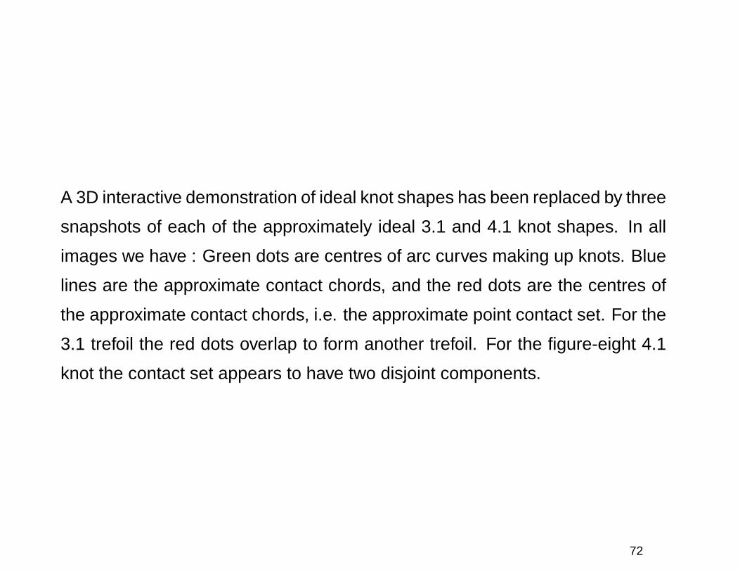
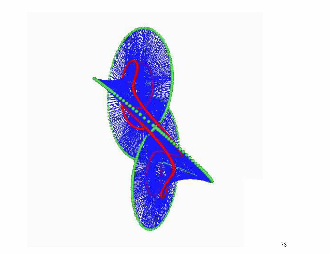
A 3D interactive demonstration of ideal knot shapes has been replaced by three

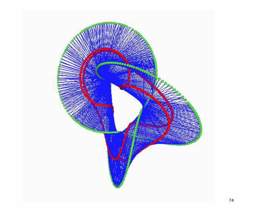
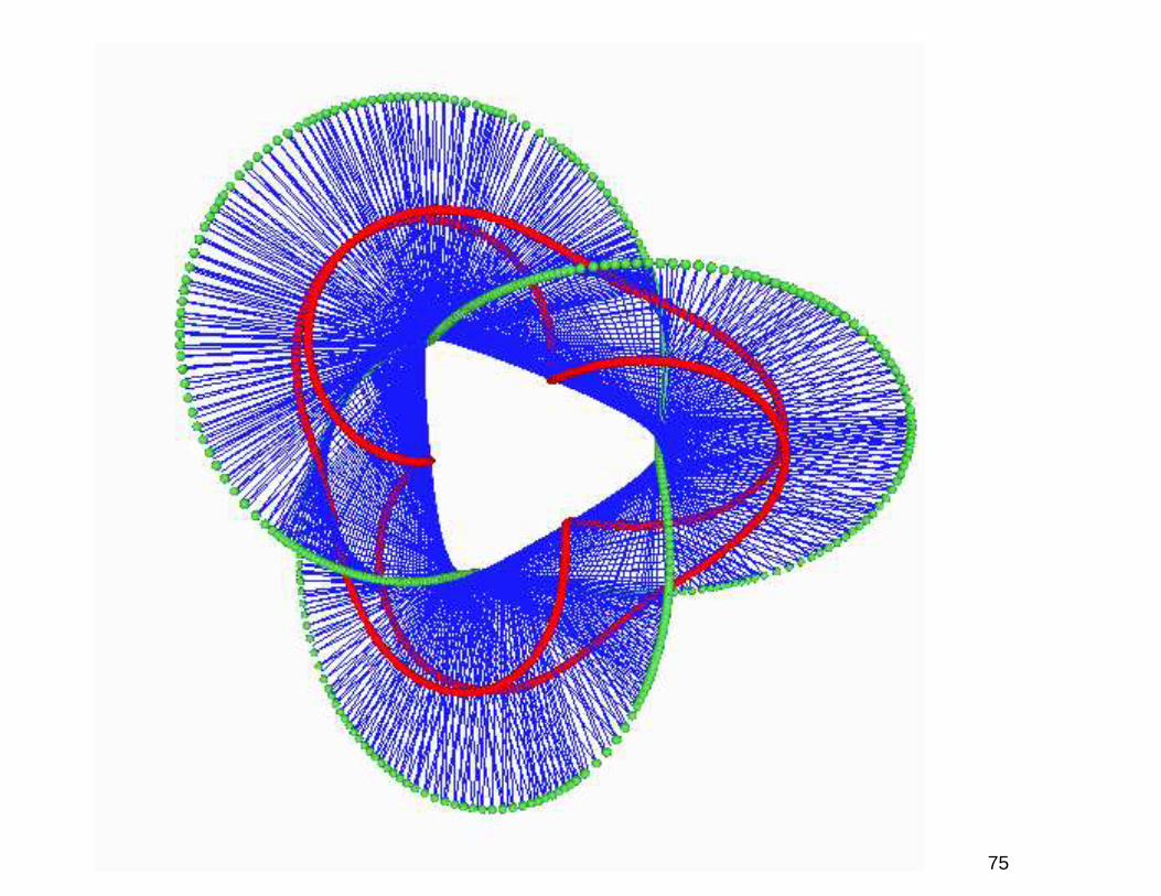
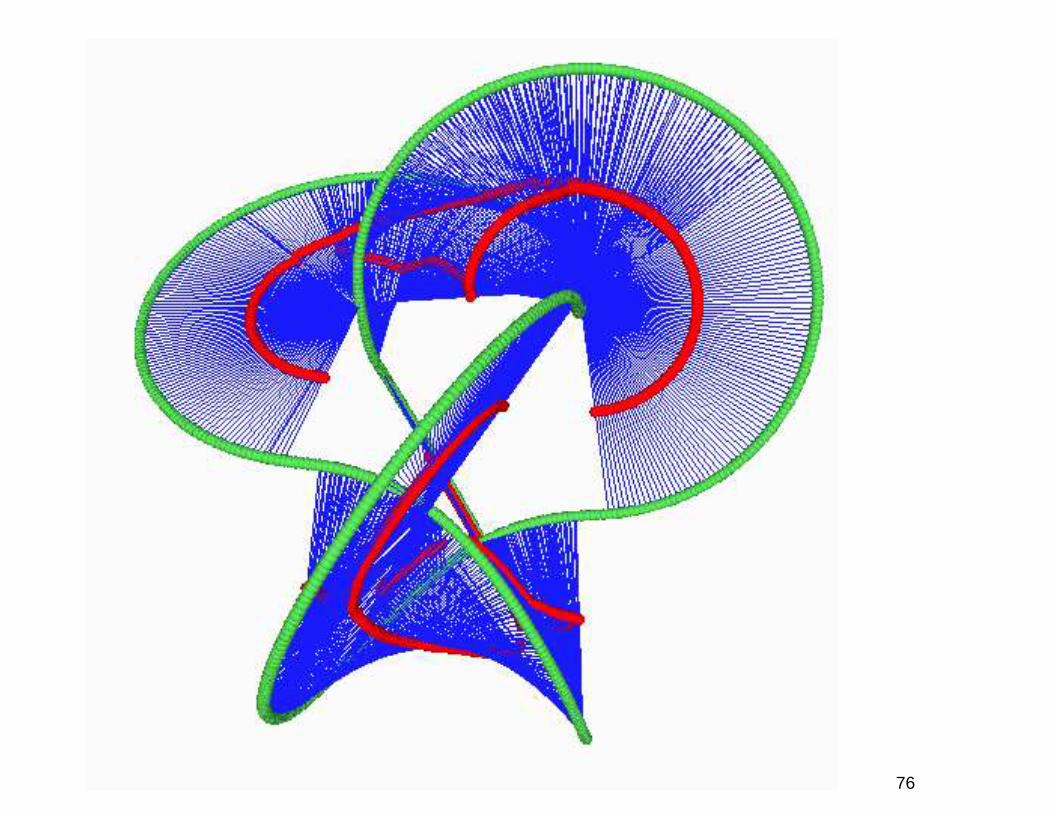
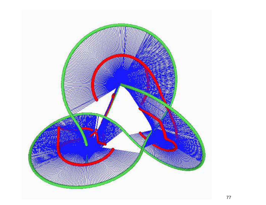
snapshots of each of the approximately ideal 3.1 and 4.1 knot shapes. In all

images we have : Green dots are centres of arc curves making up knots. Blue

lines are the approximate contact chords, and the red dots are the centres of

the approximate contact chords, i.e. the approximate point contact set. For the

3.1 trefoil the red dots overlap to form another trefoil. For the figure-eight 4.1

knot the contact set appears to have two disjoint components.

72

73

74

75

76

77

78

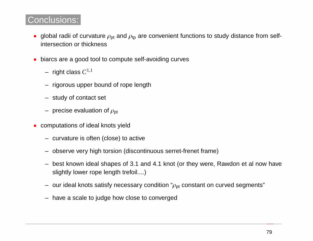
Conclusions:

• global radii of curvature ρpt and ρtp are convenient functions to study distance from self-intersection or thickness

• biarcs are a good tool to compute self-avoiding curves

– right class C1,1

– rigorous upper bound of rope length

– study of contact set

– precise evaluation of ρpt

• computations of ideal knots yield

– curvature is often (close) to active

– observe very high torsion (discontinuous serret-frenet frame)

– best known ideal shapes of 3.1 and 4.1 knot (or they were, Rawdon et al now haveslightly lower rope length trefoil....)

– our ideal knots satisfy necessary condition “ρpt constant on curved segments”

– have a scale to judge how close to converged

79

Thanks:

Merci pour l’invitation....

Merci pour votre attention...

et merci pour le support informatique :-) ....

80

Joint Work:

JHM + Oscar Gonzalez, UT-Austin

JHM + OG + Heiko von der Mosel, Aachen + Friedemann Schuricht, Cologne

JHM + OG + Jana Smutny

JS, PhD Thesis, EPFL 2004 (and the majority of these slides)

JHM + JS + Mathias Carlen, Diplomant, EPFL + Ben Laurie, London

JHM + Andrzej Stasiak, U. of Lausanne

Crucial input from: Remi Langevin, U. of Bourgogne, Arieh Iserles, U. of Cam-

bridge

81

The material of the three talks is described at length in the thesis,

Global Radii of Curvature, and the Biarc Approximation of Space Curves: In

Pursuit of Ideal Knot Shapes, by Jana Smutny

which is available in pdf as PhD Thesis number [7] on:

http://lcvmwww.epfl.ch/publis.html

and in the five articles (also available electronically from the same page):

[82] M. Carlen, B. Laurie, J.H. Maddocks, J. Smutny, ”Biarcs, Global Radius of

Curvature, and the Computation of Ideal Knot Shapes”, Chapter in ”Physical

and Numerical Models in Knot Theory and Their Application to the Life Sci-

ences”, Eds. J. Calvo, K. Millett, E. Rawdon, and A. Stasiak, To be published

by World Scientific. (A condensed version of Chapters 4, 7 and 8 of the thesis

[7])

and82

[65] O. Gonzalez, J.H. Maddocks, J. Smutny, ”Curves, circles, and spheres”,

Contemporary Mathematics 304 (2002) 195-215. (The original version of Chap-

ter 3 of the thesis [7])

[61] O. Gonzalez, J.H. Maddocks, F. Schuricht, H. von der Mosel, ”Global cur-

vature and self-contact of nonlinearly elastic curves and rods”, Calculus of Vari-

ations 14 (2002) 29-68. (A rather technical article showing how global radius of

curvature can be used to prove the existence and minimal regularity of various

optimal packing problems, including ideal knot shapes.)

[57] A. Stasiak, J. H. Maddocks, ”Best packing in proteins and DNA”, Nature

406, July (2000) 251-252. ( A discussion of an article by Maritan et al that

uses global radius of curvature in optimal packing and relates to the crystal

structures of various molecular helices.)

and

83

[43] O. Gonzalez, J.H. Maddocks, ”Global Curvature, Thickness and the Ideal

Shapes of Knots”, Proc. National Academy of Sciences of the USA 96 (1999)

4769-4773. (The original article on global radius of curvature, as motivated by

ideal knot shapes.)

84