Icarus 222 (2013) 1–19

Contents lists available at SciVerse ScienceDirect

Icarus

journal homepage: www.elsevier .com/locate / icarus

Global modelling of the early martian climate under a denser CO2

atmosphere: Water cycle and ice evolution

R. Wordsworth a,⇑, F. Forget a, E. Millour a, J.W. Head b, J.-B. Madeleine a,b, B. Charnay a

a Laboratoire de Métérologie Dynamique, Institut Pierre Simon Laplace, Paris, Franceb Department of Geological Sciences, Brown University, Providence, RI 02912, USA

a r t i c l e i n f o a b s t r a c t

Article history:Received 30 March 2012Revised 28 September 2012Accepted 29 September 2012Available online 30 October 2012

Keywords:Atmospheres, EvolutionMars, AtmosphereMars, ClimateMars, Polar geologyIces

0019-1035/$ - see front matter � 2012 Elsevier Inc. Ahttp://dx.doi.org/10.1016/j.icarus.2012.09.036

⇑ Corresponding author. Present address: DepartmUniversity of Chicago, IL 60637, USA.

E-mail address: rwordsworth@uchicago.edu (R. W

We discuss 3D global simulations of the early martian climate that we have performed assuming a faintyoung Sun and denser CO2 atmosphere. We include a self-consistent representation of the water cycle,with atmosphere–surface interactions, atmospheric transport, and the radiative effects of CO2 and H2Ogas and clouds taken into account. We find that for atmospheric pressures greater than a fraction of abar, the adiabatic cooling effect causes temperatures in the southern highland valley network regionsto fall significantly below the global average. Long-term climate evolution simulations indicate that inthese circumstances, water ice is transported to the highlands from low-lying regions for a wide rangeof orbital obliquities, regardless of the extent of the Tharsis bulge. In addition, an extended water icecap forms on the southern pole, approximately corresponding to the location of the Noachian/Hesperianera Dorsa Argentea Formation. Even for a multiple-bar CO2 atmosphere, conditions are too cold to allowlong-term surface liquid water. Limited melting occurs on warm summer days in some locations, but onlyfor surface albedo and thermal inertia conditions that may be unrealistic for water ice. Nonetheless,meteorite impacts and volcanism could potentially cause intense episodic melting under such conditions.Because ice migration to higher altitudes is a robust mechanism for recharging highland water sourcesafter such events, we suggest that this globally sub-zero, ‘icy highlands’ scenario for the late Noachianclimate may be sufficient to explain most of the fluvial geology without the need to invoke additionallong-term warming mechanisms or an early warm, wet Mars.

� 2012 Elsevier Inc. All rights reserved.

1. Introduction

After many decades of observational and theoretical research,the nature of the early martian climate remains an essentially un-solved problem. Extensive geological evidence indicates that therewas both flowing liquid water (e.g., Carr, 1995; Irwin et al., 2005;Fassett et al., 2008b; Hynek et al., 2010) and standing bodies ofwater (e.g., Fassett et al., 2008b) on the martian surface in the lateNoachian, but a comprehensive, integrated explanation for theobservations remains elusive. As the young Sun was fainter byaround 25% in the Noachian (before approx. 3.5 GYa) (Gough,1981), to date no climate model has been able to produce long-term warm, wet conditions in this period convincingly. Transientwarming events have been proposed to explain some of the obser-vations, but there is still no consensus as to their rate of occurrenceor overall importance.

The geomorphological evidence for an altered climate on earlyMars includes extensive dendritic channels across the highland

ll rights reserved.

ent of Geological Sciences,

ordsworth).

Noachian terrain (the famous ‘valley networks’) (Carr, 1996;Fassett et al., 2008b; Hynek et al., 2010), fossilised river deltas withmeandering features (Malin and Edgett, 2003; Fassett and Head,2005), records of quasi-periodic sediment deposition (Lewiset al., 2008), and regions of enhanced erosion most readily ex-plained through fluvial activity (Hynek and Phillips, 2001). Somestudies have also suggested evidence for an ancient ocean in thelow-lying northern plains. These include a global analysis of themartian hydrosphere (Clifford and Parker, 2001) and an assess-ment of river delta/valley network contact altitudes (di Achilleand Hynek, 2010). However, in the absence of other evidence,the existence of a northern ocean in the Noachian remains highlycontroversial.

More recent geochemical evidence of aqueous alteration onMars has both broadened and complicated our view of the earlyclimate. Observations by the OMEGA and CRISM instruments onthe Mars Express/Mars Reconnaissance Orbiter spacecraft (Pouletet al., 2005; Bibring et al., 2006; Mustard et al., 2008; Ehlmannet al., 2011) showed widespread evidence for phyllosilicate (�clay)and sulphate minerals across the central and southern Noachianterrain. Surface aqueous minerals are rarer in Mars’ northern low-lands, which are mostly covered by younger Hesperian-era lava

2 R. Wordsworth et al. / Icarus 222 (2013) 1–19

plains (Head et al., 2002; Salvatore et al., 2010) and outflow chan-nel effluent (Kreslavsky and Head, 2002). However, phyllosilicateshave been detected in some large northern impact craters thatpenetrated through these later deposits (Carter et al., 2010). Asthese impacts were understood to have excavated ancient Noa-chian terrain from below the lava plains, it seems plausible thataqueous alteration was once widespread in both hemispheres, onor just beneath the martian surface.

Evidence from crater counting (Fassett and Head, 2008a, 2011)suggests that valley network formation was active during the Noa-chian but ended near the Noachian-Hesperian boundary (approx.3.5 GYa in their analysis). Broadly speaking, this period overlapswith the end of the period when impacts were frequent and theTharsis rise was still forming. Interestingly, however, crater statis-tics also suggest that the main period of phyllosilicate formationended somewhat before the last valley networks were created.Few Late Noachian open-basin lakes (Fassett et al., 2008b) showevidence of extensive in situ phyllosilicates on their floors (Goudgeet al., 2012) and in those that do, the clays appear to have beentransported there from older deposits by way of valley networks(e.g., Ehlmann et al., 2008).

Interpreting the surface conditions necessary to form the ob-served phyllosilicates on Mars remains a key challenge to under-standing the Noachian climate. It is clear that there is substantialdiversity in the early martian mineralogical record, which probablyat least partially reflects progressive changes in environmentalconditions over time (Bibring et al., 2006; Mustard et al., 2008;Murchie et al., 2009; Andrews-Hanna et al., 2010; Andrews-Hannaand Lewis, 2011). Nonetheless, the most recent reviews of theavailable geochemical evidence suggest that the majority of phyl-losilicate deposits may have been formed via subsurface hydro-thermal alteration (Ehlmann et al., 2011) or episodic processes,as opposed to a long-term, warm wet climate.

While it is likely that Mars once possessed a thicker CO2 atmo-sphere than it has today, it is well known that CO2 gaseous absorp-tion alone cannot produce a greenhouse effect strong enough toallow liquid water on early Mars at any atmospheric pressure(Kasting, 1991). Various alternative explanations for an earlywarm, wet climate have been put forward. Two of the most notableare additional absorption by volcanically emitted sulphur dioxide(Halevy et al., 2007), and downward scattering of outgoing infraredradiation by CO2 clouds (Forget and Pierrehumbert, 1997). How-ever, both these hypotheses have been criticised as insufficient inlater studies (Colaprete and Toon, 2003; Tian et al., 2010).Sulphur-induced warming is attractive due to the correlationbetween the timing of Tharsis formation and the valley networksand the abundance of sulphate minerals on the martian surface.However, Tian et al. (2010) argued that this mechanism wouldbe ineffective on timescales longer than a few months due to thecooling effects of sulphate aerosol formation in the high atmo-sphere. CO2 clouds are a robust feature of cold CO2 atmospheresthat have already been observed in the mesosphere of present-day Mars (Montmessin et al., 2007). They can cause extremelyeffective warming via infrared scattering if they form at an optimalaltitude and have global coverage close to 100%. However, our 3Dsimulations of dry CO2 atmospheres (Forget et al., 2012) suggestthat their warming effect is unlikely to be strong enough to raiseglobal mean temperatures above the melting point of water forreasonable atmospheric pressures.

Given the problems with steady-state warm, wet models, otherresearchers have proposed that extreme events such as meteoriteimpacts could be capable of causing enough warming to explainthe observed erosion alone (Segura et al., 2002, 2008; Toon et al.,2010). These authors proposed that transient steam atmosphereswould form for up to several millenia as a result of impacts be-tween 30 and 250 km in diameter. They argued that the enhanced

precipitation rates under such conditions would be sufficient tocarve valley networks similar to those observed on Mars, andhence that a long-term warm climate was not necessary to explainthe geological evidence. This hypothesis has been questioned by la-ter studies – for example, landform evolution modelling of the Par-ana Valles region (�20�N, 15�W) (Barnhart et al., 2009) hassuggested that the near-absence of crater rim breaches there isindicative of a long-term, semi-arid climate, as opposed to inter-mittent catastrophic deluges. Other researchers have argued thatwith realistic values of soil erodability, there is a significant dis-crepancy (of order 104) between the estimated Noachian erosionrates and the total erosion possible due to post-impact rainfall(Jim Kasting, private communication). Hence impact-generatedsteam atmospheres alone still appear unable to explain key ele-ments of the geological observations, and the role of impacts inthe Noachian hydrological cycle in general remains unclear.

Most previous theoretical studies of the early martian climatehave used one-dimensional, globally averaged models. While suchmodels have the advantage of allowing a simple and rapid assess-ment of warming for a given atmosphere, they are incapable ofaddressing the influence of seasonal and topographic temperaturevariations on the global water cycle. Johnson et al. (2008) exam-ined the impact of sulphur volatiles on climate in a 3D general cir-culation model (GCM), but they did not include a dynamic watercycle or the radiative effects of clouds or aerosols. To our knowl-edge, no other study has yet attempted to model the primitivemartian climate in a 3D GCM.

Here we describe a range of three-dimensional simulations wehave performed to investigate possible climate scenarios on earlyMars. Our approach has been to study only the simplest possibleatmospheric compositions, but to treat all physical processes asaccurately as possible. We modelled the early martian climate in3D under a denser CO2 atmosphere with (a) dynamical representa-tion of cloud formation and radiative effects (CO2 and H2O), (b)self-consistent, integrated representation of the water cycle and(c) accurate parameterisation of dense CO2 radiative transfer. Wehave studied the effects of varying atmospheric pressure, orbitalobliquity, surface topography and starting H2O inventory. In acompanion paper (Forget et al., 2012), we describe the climate un-der dry (pure CO2) conditions. Here we focus on the water cycle,including its effects on global climate and long-term surface icestabilization. Based on our results, we propose a new hypothesisfor valley network formation that combines aspects of previoussteady-state and transient warming theories.

In Section 2, we describe our climate model, including the radi-ative transfer and dynamical modules and assumptions on thewater cycle and cloud formation. In Section 3, we describe the re-sults. First, 100% relative humidity simulations are analysed andcompared with results assuming a dry atmosphere (Forget et al.,2012). Next, simulations with a self-consistent water cycle andvarying assumptions on the initial CO2 and H2O inventories andsurface topography are described. Particular emphasis is placedon (a) the long-term evolution of the global hydrology towards asteady state and (b) local melting due to short-term transient heat-ing events. In Section 4 we discuss our results in the context of con-straints from geological observations and atmospheric evolutiontheory, and assess the probable effects of impacts during a periodof higher flux. Finally, we describe what we view as the most likelyscenario for valley network formation in the late Noachian andsuggest a few directions for future study.

2. Method

To produce our results we used the LMD Generic Climate Model,a new climate simulator with generalised radiative transfer and

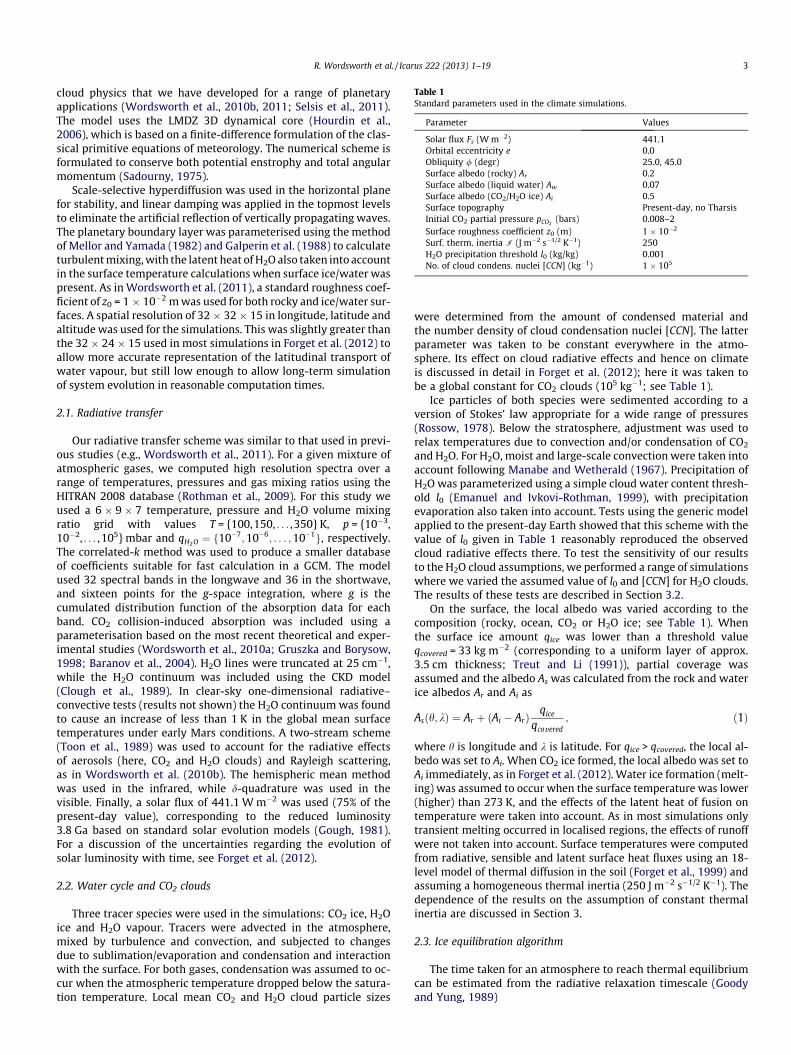
Table 1Standard parameters used in the climate simulations.

Parameter Values

Solar flux Fs (W m�2) 441.1Orbital eccentricity e 0.0Obliquity / (degr) 25.0, 45.0Surface albedo (rocky) Ar 0.2Surface albedo (liquid water) Aw 0.07Surface albedo (CO2/H2O ice) Ai 0.5Surface topography Present-day, no TharsisInitial CO2 partial pressure pCO2

(bars) 0.008–2Surface roughness coefficient z0 (m) 1 � 10�2

Surf. therm. inertia I (J m�2 s�1/2 K�1) 250H2O precipitation threshold l0 (kg/kg) 0.001No. of cloud condens. nuclei [CCN] (kg�1) 1 � 105

R. Wordsworth et al. / Icarus 222 (2013) 1–19 3

cloud physics that we have developed for a range of planetaryapplications (Wordsworth et al., 2010b, 2011; Selsis et al., 2011).The model uses the LMDZ 3D dynamical core (Hourdin et al.,2006), which is based on a finite-difference formulation of the clas-sical primitive equations of meteorology. The numerical scheme isformulated to conserve both potential enstrophy and total angularmomentum (Sadourny, 1975).

Scale-selective hyperdiffusion was used in the horizontal planefor stability, and linear damping was applied in the topmost levelsto eliminate the artificial reflection of vertically propagating waves.The planetary boundary layer was parameterised using the methodof Mellor and Yamada (1982) and Galperin et al. (1988) to calculateturbulent mixing, with the latent heat of H2O also taken into accountin the surface temperature calculations when surface ice/water waspresent. As in Wordsworth et al. (2011), a standard roughness coef-ficient of z0 = 1 � 10�2 m was used for both rocky and ice/water sur-faces. A spatial resolution of 32 � 32 � 15 in longitude, latitude andaltitude was used for the simulations. This was slightly greater thanthe 32 � 24 � 15 used in most simulations in Forget et al. (2012) toallow more accurate representation of the latitudinal transport ofwater vapour, but still low enough to allow long-term simulationof system evolution in reasonable computation times.

2.1. Radiative transfer

Our radiative transfer scheme was similar to that used in previ-ous studies (e.g., Wordsworth et al., 2011). For a given mixture ofatmospheric gases, we computed high resolution spectra over arange of temperatures, pressures and gas mixing ratios using theHITRAN 2008 database (Rothman et al., 2009). For this study weused a 6 � 9 � 7 temperature, pressure and H2O volume mixingratio grid with values T = {100,150, . . . ,350} K, p = {10�3,10�2, . . . ,105} mbar and qH2O ¼ f10�7;10�6; . . . ;10�1g, respectively.The correlated-k method was used to produce a smaller databaseof coefficients suitable for fast calculation in a GCM. The modelused 32 spectral bands in the longwave and 36 in the shortwave,and sixteen points for the g-space integration, where g is thecumulated distribution function of the absorption data for eachband. CO2 collision-induced absorption was included using aparameterisation based on the most recent theoretical and exper-imental studies (Wordsworth et al., 2010a; Gruszka and Borysow,1998; Baranov et al., 2004). H2O lines were truncated at 25 cm�1,while the H2O continuum was included using the CKD model(Clough et al., 1989). In clear-sky one-dimensional radiative–convective tests (results not shown) the H2O continuum was foundto cause an increase of less than 1 K in the global mean surfacetemperatures under early Mars conditions. A two-stream scheme(Toon et al., 1989) was used to account for the radiative effectsof aerosols (here, CO2 and H2O clouds) and Rayleigh scattering,as in Wordsworth et al. (2010b). The hemispheric mean methodwas used in the infrared, while d-quadrature was used in thevisible. Finally, a solar flux of 441.1 W m�2 was used (75% of thepresent-day value), corresponding to the reduced luminosity3.8 Ga based on standard solar evolution models (Gough, 1981).For a discussion of the uncertainties regarding the evolution ofsolar luminosity with time, see Forget et al. (2012).

2.2. Water cycle and CO2 clouds

Three tracer species were used in the simulations: CO2 ice, H2Oice and H2O vapour. Tracers were advected in the atmosphere,mixed by turbulence and convection, and subjected to changesdue to sublimation/evaporation and condensation and interactionwith the surface. For both gases, condensation was assumed to oc-cur when the atmospheric temperature dropped below the satura-tion temperature. Local mean CO2 and H2O cloud particle sizes

were determined from the amount of condensed material andthe number density of cloud condensation nuclei [CCN]. The latterparameter was taken to be constant everywhere in the atmo-sphere. Its effect on cloud radiative effects and hence on climateis discussed in detail in Forget et al. (2012); here it was taken tobe a global constant for CO2 clouds (105 kg�1; see Table 1).

Ice particles of both species were sedimented according to aversion of Stokes’ law appropriate for a wide range of pressures(Rossow, 1978). Below the stratosphere, adjustment was used torelax temperatures due to convection and/or condensation of CO2

and H2O. For H2O, moist and large-scale convection were taken intoaccount following Manabe and Wetherald (1967). Precipitation ofH2O was parameterized using a simple cloud water content thresh-old l0 (Emanuel and Ivkovi-Rothman, 1999), with precipitationevaporation also taken into account. Tests using the generic modelapplied to the present-day Earth showed that this scheme with thevalue of l0 given in Table 1 reasonably reproduced the observedcloud radiative effects there. To test the sensitivity of our resultsto the H2O cloud assumptions, we performed a range of simulationswhere we varied the assumed value of l0 and [CCN] for H2O clouds.The results of these tests are described in Section 3.2.

On the surface, the local albedo was varied according to thecomposition (rocky, ocean, CO2 or H2O ice; see Table 1). Whenthe surface ice amount qice was lower than a threshold valueqcovered = 33 kg m�2 (corresponding to a uniform layer of approx.3.5 cm thickness; Treut and Li (1991)), partial coverage wasassumed and the albedo As was calculated from the rock and waterice albedos Ar and Ai as

Asðh; kÞ ¼ Ar þ ðAi � ArÞqice

qcovered; ð1Þ

where h is longitude and k is latitude. For qice > qcovered, the local al-bedo was set to Ai. When CO2 ice formed, the local albedo was set toAi immediately, as in Forget et al. (2012). Water ice formation (melt-ing) was assumed to occur when the surface temperature was lower(higher) than 273 K, and the effects of the latent heat of fusion ontemperature were taken into account. As in most simulations onlytransient melting occurred in localised regions, the effects of runoffwere not taken into account. Surface temperatures were computedfrom radiative, sensible and latent surface heat fluxes using an 18-level model of thermal diffusion in the soil (Forget et al., 1999) andassuming a homogeneous thermal inertia (250 J m�2 s�1/2 K�1). Thedependence of the results on the assumption of constant thermalinertia are discussed in Section 3.

2.3. Ice equilibration algorithm

The time taken for an atmosphere to reach thermal equilibriumcan be estimated from the radiative relaxation timescale (Goodyand Yung, 1989)

o o o o o o o180 W 120 W 60 W 0 60 E 120 E 180 W 80oS

40oS

0o

40oN

80oN

o o o o o o o180 W 120 W 60 W 0 60 E 120 E 180 W 80oS

40oS

0o

40oN

80 oN

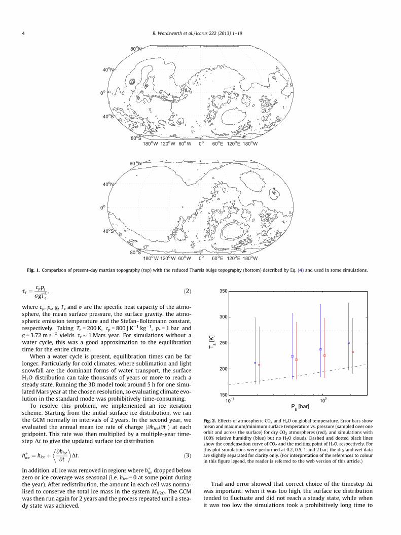
Fig. 1. Comparison of present-day martian topography (top) with the reduced Tharsis bulge topography (bottom) described by Eq. (4) and used in some simulations.

10 1 100150

200

250

300

350

T s [K]

Ps [bar]

Fig. 2. Effects of atmospheric CO2 and H2O on global temperature. Error bars showmean and maximum/minimum surface temperature vs. pressure (sampled over oneorbit and across the surface) for dry CO2 atmospheres (red), and simulations with100% relative humidity (blue) but no H2O clouds. Dashed and dotted black linesshow the condensation curve of CO2 and the melting point of H2O, respectively. Forthis plot simulations were performed at 0.2, 0.5, 1 and 2 bar; the dry and wet dataare slightly separated for clarity only. (For interpretation of the references to colourin this figure legend, the reader is referred to the web version of this article.)

4 R. Wordsworth et al. / Icarus 222 (2013) 1–19

sr ¼cpps

rgT3e

; ð2Þ

where cp, ps, g, Te and r are the specific heat capacity of the atmo-sphere, the mean surface pressure, the surface gravity, the atmo-spheric emission temperature and the Stefan–Boltzmann constant,respectively. Taking Te = 200 K, cp = 800 J K�1 kg�1, ps = 1 bar andg = 3.72 m s�2 yields sr � 1 Mars year. For simulations without awater cycle, this was a good approximation to the equilibrationtime for the entire climate.

When a water cycle is present, equilibration times can be farlonger. Particularly for cold climates, where sublimation and lightsnowfall are the dominant forms of water transport, the surfaceH2O distribution can take thousands of years or more to reach asteady state. Running the 3D model took around 5 h for one simu-lated Mars year at the chosen resolution, so evaluating climate evo-lution in the standard mode was prohibitively time-consuming.

To resolve this problem, we implemented an ice iterationscheme. Starting from the initial surface ice distribution, we ranthe GCM normally in intervals of 2 years. In the second year, weevaluated the annual mean ice rate of change h@hice/@t i at eachgridpoint. This rate was then multiplied by a multiple-year time-step Dt to give the updated surface ice distribution

hþice ¼ hice þ@hice

@t

� �Dt: ð3Þ

In addition, all ice was removed in regions where hþice dropped belowzero or ice coverage was seasonal (i.e. hice = 0 at some point duringthe year). After redistribution, the amount in each cell was norma-lised to conserve the total ice mass in the system MH2O. The GCMwas then run again for 2 years and the process repeated until a stea-dy state was achieved.

Trial and error showed that correct choice of the timestep Dtwas important: when it was too high, the surface ice distributiontended to fluctuate and did not reach a steady state, while whenit was too low the simulations took a prohibitively long time to

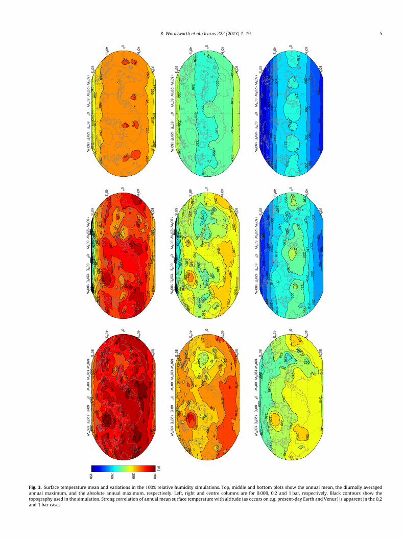
Fig. 3. Surface temperature mean and variations in the 100% relative humidity simulations. Top, middle and bottom plots show the annual mean, the diurnally averagedannual maximum, and the absolute annual maximum, respectively. Left, right and centre columns are for 0.008, 0.2 and 1 bar, respectively. Black contours show thetopography used in the simulation. Strong correlation of annual mean surface temperature with altitude (as occurs on e.g. present-day Earth and Venus) is apparent in the 0.2and 1 bar cases.

R. Wordsworth et al. / Icarus 222 (2013) 1–19 5

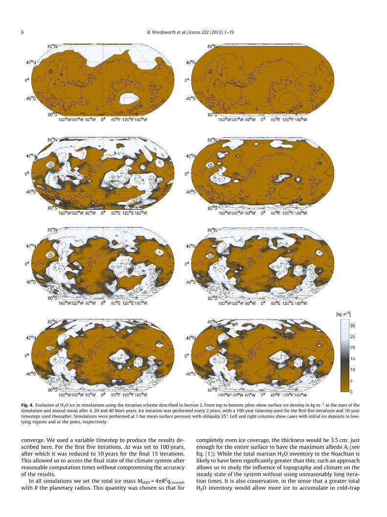
Fig. 4. Evolution of H2O ice in simulations using the iteration scheme described in Section 2. From top to bottom, plots show surface ice density in kg m�2 at the start of thesimulation and annual mean after 4, 20 and 40 Mars years. Ice iteration was performed every 2 years, with a 100-year timestep used for the first five iterations and 10-yeartimesteps used thereafter. Simulations were performed at 1 bar mean surface pressure with obliquity 25�. Left and right columns show cases with initial ice deposits in low-lying regions and at the poles, respectively.

6 R. Wordsworth et al. / Icarus 222 (2013) 1–19

converge. We used a variable timestep to produce the results de-scribed here. For the first five iterations, Dt was set to 100 years,after which it was reduced to 10 years for the final 15 iterations.This allowed us to access the final state of the climate system afterreasonable computation times without compromising the accuracyof the results.

In all simulations we set the total ice mass MH2O = 4pR2qcovered,with R the planetary radius. This quantity was chosen so that for

completely even ice coverage, the thickness would be 3.5 cm: justenough for the entire surface to have the maximum albedo Ai (seeEq. (1)). While the total martian H2O inventory in the Noachian islikely to have been significantly greater than this, such an approachallows us to study the influence of topography and climate on thesteady state of the system without using unreasonably long itera-tion times. It is also conservative, in the sense that a greater totalH2O inventory would allow more ice to accumulate in cold-trap

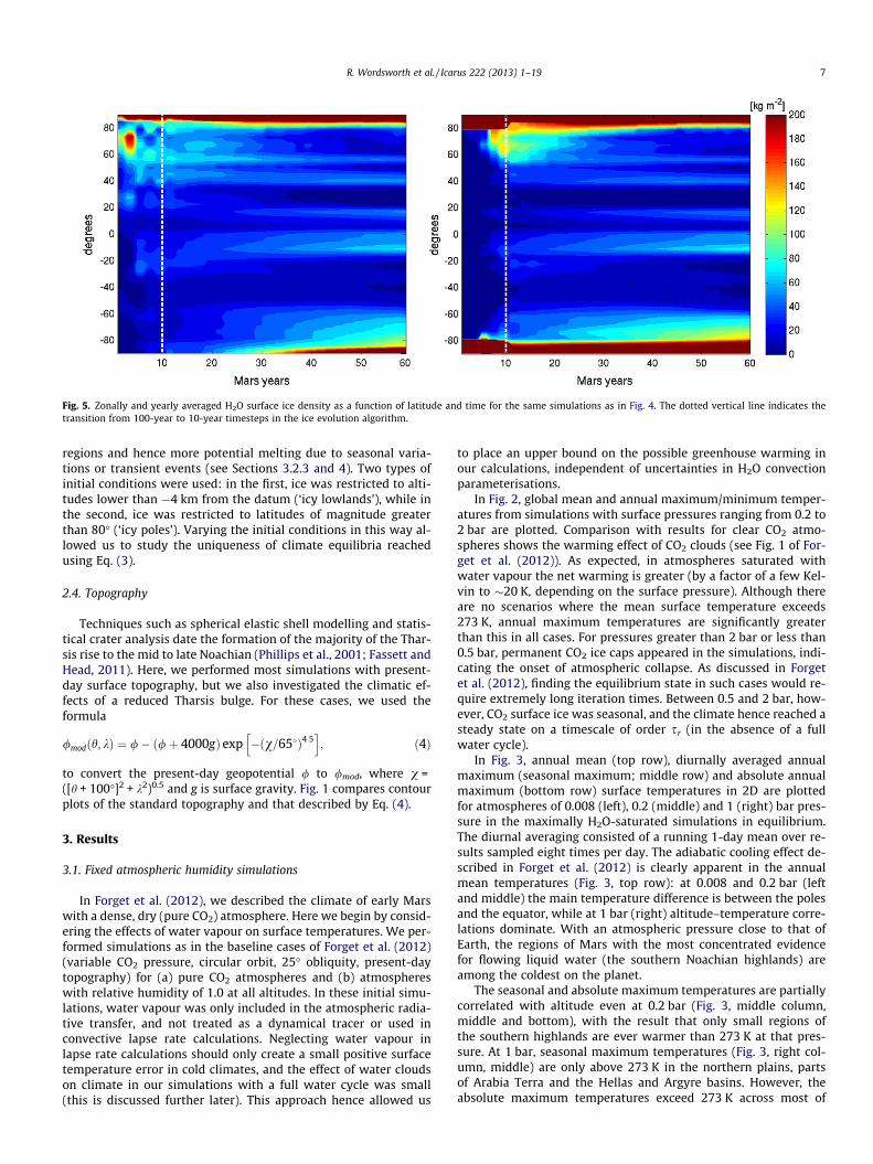
Fig. 5. Zonally and yearly averaged H2O surface ice density as a function of latitude and time for the same simulations as in Fig. 4. The dotted vertical line indicates thetransition from 100-year to 10-year timesteps in the ice evolution algorithm.

R. Wordsworth et al. / Icarus 222 (2013) 1–19 7

regions and hence more potential melting due to seasonal varia-tions or transient events (see Sections 3.2.3 and 4). Two types ofinitial conditions were used: in the first, ice was restricted to alti-tudes lower than �4 km from the datum (‘icy lowlands’), while inthe second, ice was restricted to latitudes of magnitude greaterthan 80� (‘icy poles’). Varying the initial conditions in this way al-lowed us to study the uniqueness of climate equilibria reachedusing Eq. (3).

2.4. Topography

Techniques such as spherical elastic shell modelling and statis-tical crater analysis date the formation of the majority of the Thar-sis rise to the mid to late Noachian (Phillips et al., 2001; Fassett andHead, 2011). Here, we performed most simulations with present-day surface topography, but we also investigated the climatic ef-fects of a reduced Tharsis bulge. For these cases, we used theformula

/modðh; kÞ ¼ /� ð/þ 4000gÞ exp �ðv=65�Þ4:5h i

; ð4Þ

to convert the present-day geopotential / to /mod, where v =([h + 100�]2 + k2)0.5 and g is surface gravity. Fig. 1 compares contourplots of the standard topography and that described by Eq. (4).

3. Results

3.1. Fixed atmospheric humidity simulations

In Forget et al. (2012), we described the climate of early Marswith a dense, dry (pure CO2) atmosphere. Here we begin by consid-ering the effects of water vapour on surface temperatures. We per-formed simulations as in the baseline cases of Forget et al. (2012)(variable CO2 pressure, circular orbit, 25� obliquity, present-daytopography) for (a) pure CO2 atmospheres and (b) atmosphereswith relative humidity of 1.0 at all altitudes. In these initial simu-lations, water vapour was only included in the atmospheric radia-tive transfer, and not treated as a dynamical tracer or used inconvective lapse rate calculations. Neglecting water vapour inlapse rate calculations should only create a small positive surfacetemperature error in cold climates, and the effect of water cloudson climate in our simulations with a full water cycle was small(this is discussed further later). This approach hence allowed us

to place an upper bound on the possible greenhouse warming inour calculations, independent of uncertainties in H2O convectionparameterisations.

In Fig. 2, global mean and annual maximum/minimum temper-atures from simulations with surface pressures ranging from 0.2 to2 bar are plotted. Comparison with results for clear CO2 atmo-spheres shows the warming effect of CO2 clouds (see Fig. 1 of For-get et al. (2012)). As expected, in atmospheres saturated withwater vapour the net warming is greater (by a factor of a few Kel-vin to �20 K, depending on the surface pressure). Although thereare no scenarios where the mean surface temperature exceeds273 K, annual maximum temperatures are significantly greaterthan this in all cases. For pressures greater than 2 bar or less than0.5 bar, permanent CO2 ice caps appeared in the simulations, indi-cating the onset of atmospheric collapse. As discussed in Forgetet al. (2012), finding the equilibrium state in such cases would re-quire extremely long iteration times. Between 0.5 and 2 bar, how-ever, CO2 surface ice was seasonal, and the climate hence reached asteady state on a timescale of order sr (in the absence of a fullwater cycle).

In Fig. 3, annual mean (top row), diurnally averaged annualmaximum (seasonal maximum; middle row) and absolute annualmaximum (bottom row) surface temperatures in 2D are plottedfor atmospheres of 0.008 (left), 0.2 (middle) and 1 (right) bar pres-sure in the maximally H2O-saturated simulations in equilibrium.The diurnal averaging consisted of a running 1-day mean over re-sults sampled eight times per day. The adiabatic cooling effect de-scribed in Forget et al. (2012) is clearly apparent in the annualmean temperatures (Fig. 3, top row): at 0.008 and 0.2 bar (leftand middle) the main temperature difference is between the polesand the equator, while at 1 bar (right) altitude–temperature corre-lations dominate. With an atmospheric pressure close to that ofEarth, the regions of Mars with the most concentrated evidencefor flowing liquid water (the southern Noachian highlands) areamong the coldest on the planet.

The seasonal and absolute maximum temperatures are partiallycorrelated with altitude even at 0.2 bar (Fig. 3, middle column,middle and bottom), with the result that only small regions ofthe southern highlands are ever warmer than 273 K at that pres-sure. At 1 bar, seasonal maximum temperatures (Fig. 3, right col-umn, middle) are only above 273 K in the northern plains, partsof Arabia Terra and the Hellas and Argyre basins. However, theabsolute maximum temperatures exceed 273 K across most of

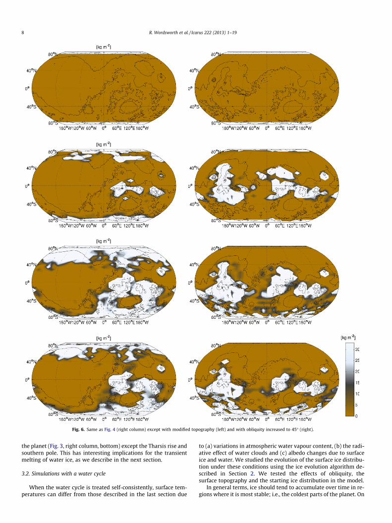
Fig. 6. Same as Fig. 4 (right column) except with modified topography (left) and with obliquity increased to 45� (right).

8 R. Wordsworth et al. / Icarus 222 (2013) 1–19

the planet (Fig. 3, right column, bottom) except the Tharsis rise andsouthern pole. This has interesting implications for the transientmelting of water ice, as we describe in the next section.

3.2. Simulations with a water cycle

When the water cycle is treated self-consistently, surface tem-peratures can differ from those described in the last section due

to (a) variations in atmospheric water vapour content, (b) the radi-ative effect of water clouds and (c) albedo changes due to surfaceice and water. We studied the evolution of the surface ice distribu-tion under these conditions using the ice evolution algorithm de-scribed in Section 2. We tested the effects of obliquity, thesurface topography and the starting ice distribution in the model.

In general terms, ice should tend to accumulate over time in re-gions where it is most stable; i.e., the coldest parts of the planet. On

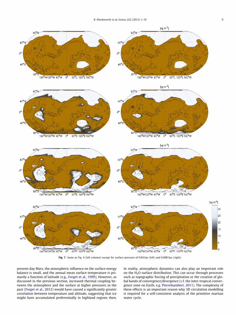
Fig. 7. Same as Fig. 4 (left column) except for surface pressure of 0.04 bar (left) and 0.008 bar (right).

R. Wordsworth et al. / Icarus 222 (2013) 1–19 9

present-day Mars, the atmospheric influence on the surface energybalance is small, and the annual mean surface temperature is pri-marily a function of latitude (e.g., Forget et al., 1999). However, asdiscussed in the previous section, increased thermal coupling be-tween the atmosphere and the surface at higher pressures in thepast (Forget et al., 2012) would have caused a significantly greatercorrelation between temperature and altitude, suggesting that icemight have accumulated preferentially in highland regions then.

In reality, atmospheric dynamics can also play an important roleon the H2O surface distribution. This can occur through processessuch as topographic forcing of precipitation or the creation of glo-bal bands of convergence/divergence (c.f. the inter-tropical conver-gence zone on Earth, e.g. Pierrehumbert, 2011). The complexity ofthese effects is an important reason why 3D circulation modellingis required for a self-consistent analysis of the primitive martianwater cycle.

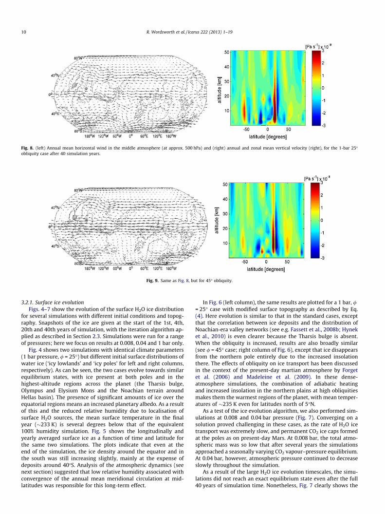
Fig. 8. (left) Annual mean horizontal wind in the middle atmosphere (at approx. 500 hPa) and (right) annual and zonal mean vertical velocity (right), for the 1-bar 25�obliquity case after 40 simulation years.

Fig. 9. Same as Fig. 8, but for 45� obliquity.

10 R. Wordsworth et al. / Icarus 222 (2013) 1–19

3.2.1. Surface ice evolutionFigs. 4–7 show the evolution of the surface H2O ice distribution

for several simulations with different initial conditions and topog-raphy. Snapshots of the ice are given at the start of the 1st, 4th,20th and 40th years of simulation, with the iteration algorithm ap-plied as described in Section 2.3. Simulations were run for a rangeof pressures; here we focus on results at 0.008, 0.04 and 1 bar only.

Fig. 4 shows two simulations with identical climate parameters(1 bar pressure, / = 25�) but different initial surface distributions ofwater ice (‘icy lowlands’ and ‘icy poles’ for left and right columns,respectively). As can be seen, the two cases evolve towards similarequilibrium states, with ice present at both poles and in thehighest-altitude regions across the planet (the Tharsis bulge,Olympus and Elysium Mons and the Noachian terrain aroundHellas basin). The presence of significant amounts of ice over theequatorial regions means an increased planetary albedo. As a resultof this and the reduced relative humidity due to localisation ofsurface H2O sources, the mean surface temperature in the finalyear (�233 K) is several degrees below that of the equivalent100% humidity simulation. Fig. 5 shows the longitudinally andyearly averaged surface ice as a function of time and latitude forthe same two simulations. The plots indicate that even at theend of the simulation, the ice density around the equator and inthe south was still increasing slightly, mainly at the expense ofdeposits around 40�S. Analysis of the atmospheric dynamics (seenext section) suggested that low relative humidity associated withconvergence of the annual mean meridional circulation at mid-latitudes was responsible for this long-term effect.

In Fig. 6 (left column), the same results are plotted for a 1 bar, /= 25� case with modified surface topography as described by Eq.(4). Here evolution is similar to that in the standard cases, exceptthat the correlation between ice deposits and the distribution ofNoachian-era valley networks (see e.g. Fassett et al., 2008b; Hyneket al., 2010) is even clearer because the Tharsis bulge is absent.When the obliquity is increased, results are also broadly similar(see / = 45� case; right column of Fig. 6), except that ice disappearsfrom the northern pole entirely due to the increased insolationthere. The effects of obliquity on ice transport has been discussedin the context of the present-day martian atmosphere by Forgetet al. (2006) and Madeleine et al. (2009). In these dense-atmosphere simulations, the combination of adiabatic heatingand increased insolation in the northern plains at high obliquitiesmakes them the warmest regions of the planet, with mean temper-atures of �235 K even for latitudes north of 5�N.

As a test of the ice evolution algorithm, we also performed sim-ulations at 0.008 and 0.04 bar pressure (Fig. 7). Converging on asolution proved challenging in these cases, as the rate of H2O icetransport was extremely slow, and permanent CO2 ice caps formedat the poles as on present-day Mars. At 0.008 bar, the total atmo-spheric mass was so low that after several years the simulationsapproached a seasonally varying CO2 vapour–pressure equilibrium.At 0.04 bar, however, atmospheric pressure continued to decreaseslowly throughout the simulation.

As a result of the large H2O ice evolution timescales, the simu-lations did not reach an exact equilibrium state even after the full40 years of simulation time. Nonetheless, Fig. 7 clearly shows the

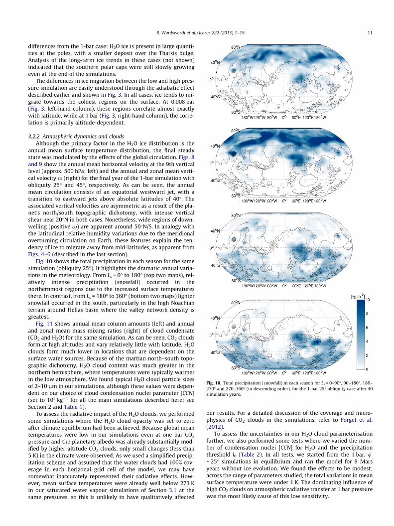
Fig. 10. Total precipitation (snowfall) in each season for Ls = 0–90�, 90–180�, 180–270� and 270–360� (in descending order), for the 1-bar 25� obliquity case after 40simulation years.

R. Wordsworth et al. / Icarus 222 (2013) 1–19 11

differences from the 1-bar case: H2O ice is present in large quanti-ties at the poles, with a smaller deposit over the Tharsis bulge.Analysis of the long-term ice trends in these cases (not shown)indicated that the southern polar caps were still slowly growingeven at the end of the simulations.

The differences in ice migration between the low and high pres-sure simulation are easily understood through the adiabatic effectdescribed earlier and shown in Fig. 3. In all cases, ice tends to mi-grate towards the coldest regions on the surface. At 0.008 bar(Fig. 3, left-hand column), these regions correlate almost exactlywith latitude, while at 1 bar (Fig. 3, right-hand column), the corre-lation is primarily altitude-dependent.

3.2.2. Atmospheric dynamics and cloudsAlthough the primary factor in the H2O ice distribution is the

annual mean surface temperature distribution, the final steadystate was modulated by the effects of the global circulation. Figs. 8and 9 show the annual mean horizontal velocity at the 9th verticallevel (approx. 500 hPa; left) and the annual and zonal mean verti-cal velocity x (right) for the final year of the 1-bar simulation withobliquity 25� and 45�, respectively. As can be seen, the annualmean circulation consists of an equatorial westward jet, with atransition to eastward jets above absolute latitudes of 40�. Theassociated vertical velocities are asymmetric as a result of the pla-net’s north/south topographic dichotomy, with intense verticalshear near 20�N in both cases. Nonetheless, wide regions of down-welling (positive x) are apparent around 50�N/S. In analogy withthe latitudinal relative humidity variations due to the meridionaloverturning circulation on Earth, these features explain the ten-dency of ice to migrate away from mid-latitudes, as apparent fromFigs. 4–6 (described in the last section).

Fig. 10 shows the total precipitation in each season for the samesimulation (obliquity 25�). It highlights the dramatic annual varia-tions in the meteorology. From Ls = 0� to 180� (top two maps), rel-atively intense precipitation (snowfall) occurred in thenorthernmost regions due to the increased surface temperaturesthere. In contrast, from Ls = 180� to 360� (bottom two maps) lightersnowfall occurred in the south, particularly in the high Noachianterrain around Hellas basin where the valley network density isgreatest.

Fig. 11 shows annual mean column amounts (left) and annualand zonal mean mass mixing ratios (right) of cloud condensate(CO2 and H2O) for the same simulation. As can be seen, CO2 cloudsform at high altitudes and vary relatively little with latitude. H2Oclouds form much lower in locations that are dependent on thesurface water sources. Because of the martian north–south topo-graphic dichotomy, H2O cloud content was much greater in thenorthern hemisphere, where temperatures were typically warmerin the low atmosphere. We found typical H2O cloud particle sizesof 2–10 lm in our simulations, although these values were depen-dent on our choice of cloud condensation nuclei parameter [CCN](set to 105 kg�1 for all the main simulations described here; seeSection 2 and Table 1).

To assess the radiative impact of the H2O clouds, we performedsome simulations where the H2O cloud opacity was set to zeroafter climate equilibrium had been achieved. Because global meantemperatures were low in our simulations even at one bar CO2

pressure and the planetary albedo was already substantially mod-ified by higher-altitude CO2 clouds, only small changes (less than5 K) in the climate were observed. As we used a simplified precip-itation scheme and assumed that the water clouds had 100% cov-erage in each horizonal grid cell of the model, we may havesomewhat inaccurately represented their radiative effects. How-ever, mean surface temperatures were already well below 273 Kin our saturated water vapour simulations of Section 3.1 at thesame pressures, so this is unlikely to have qualitatively affected

our results. For a detailed discussion of the coverage and micro-physics of CO2 clouds in the simulations, refer to Forget et al.(2012).

To assess the uncertainties in our H2O cloud parameterisationfurther, we also performed some tests where we varied the num-ber of condensation nuclei [CCN] for H2O and the precipitationthreshold l0 (Table 2). In all tests, we started from the 1 bar, /= 25� simulations in equilibrium and ran the model for 8 Marsyears without ice evolution. We found the effects to be modest;across the range of parameters studied, the total variations in meansurface temperature were under 1 K. The dominating influence ofhigh CO2 clouds on atmospheric radiative transfer at 1 bar pressurewas the most likely cause of this low sensitivity.

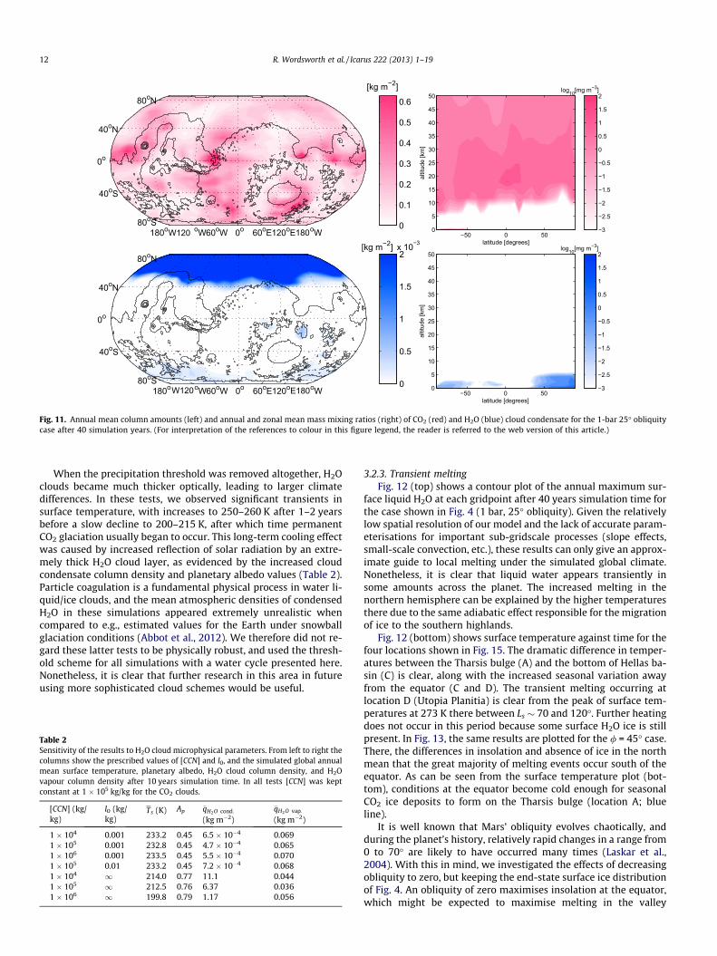
Fig. 11. Annual mean column amounts (left) and annual and zonal mean mass mixing ratios (right) of CO2 (red) and H2O (blue) cloud condensate for the 1-bar 25� obliquitycase after 40 simulation years. (For interpretation of the references to colour in this figure legend, the reader is referred to the web version of this article.)

12 R. Wordsworth et al. / Icarus 222 (2013) 1–19

When the precipitation threshold was removed altogether, H2Oclouds became much thicker optically, leading to larger climatedifferences. In these tests, we observed significant transients insurface temperature, with increases to 250–260 K after 1–2 yearsbefore a slow decline to 200–215 K, after which time permanentCO2 glaciation usually began to occur. This long-term cooling effectwas caused by increased reflection of solar radiation by an extre-mely thick H2O cloud layer, as evidenced by the increased cloudcondensate column density and planetary albedo values (Table 2).Particle coagulation is a fundamental physical process in water li-quid/ice clouds, and the mean atmospheric densities of condensedH2O in these simulations appeared extremely unrealistic whencompared to e.g., estimated values for the Earth under snowballglaciation conditions (Abbot et al., 2012). We therefore did not re-gard these latter tests to be physically robust, and used the thresh-old scheme for all simulations with a water cycle presented here.Nonetheless, it is clear that further research in this area in futureusing more sophisticated cloud schemes would be useful.

Table 2Sensitivity of the results to H2O cloud microphysical parameters. From left to right thecolumns show the prescribed values of [CCN] and l0, and the simulated global annualmean surface temperature, planetary albedo, H2O cloud column density, and H2Ovapour column density after 10 years simulation time. In all tests [CCN] was keptconstant at 1 � 105 kg/kg for the CO2 clouds.

[CCN] (kg/kg)

l0 (kg/kg)

Ts (K) Ap �qH2O cond:

(kg m�2)

�qH2O vap:

(kg m�2)

1 � 104 0.001 233.2 0.45 6.5 � 10�4 0.0691 � 105 0.001 232.8 0.45 4.7 � 10�4 0.0651 � 106 0.001 233.5 0.45 5.5 � 10�4 0.0701 � 105 0.01 233.2 0.45 7.2 � 10�4 0.0681 � 104 1 214.0 0.77 11.1 0.0441 � 105 1 212.5 0.76 6.37 0.0361 � 106 1 199.8 0.79 1.17 0.056

3.2.3. Transient meltingFig. 12 (top) shows a contour plot of the annual maximum sur-

face liquid H2O at each gridpoint after 40 years simulation time forthe case shown in Fig. 4 (1 bar, 25� obliquity). Given the relativelylow spatial resolution of our model and the lack of accurate param-eterisations for important sub-gridscale processes (slope effects,small-scale convection, etc.), these results can only give an approx-imate guide to local melting under the simulated global climate.Nonetheless, it is clear that liquid water appears transiently insome amounts across the planet. The increased melting in thenorthern hemisphere can be explained by the higher temperaturesthere due to the same adiabatic effect responsible for the migrationof ice to the southern highlands.

Fig. 12 (bottom) shows surface temperature against time for thefour locations shown in Fig. 15. The dramatic difference in temper-atures between the Tharsis bulge (A) and the bottom of Hellas ba-sin (C) is clear, along with the increased seasonal variation awayfrom the equator (C and D). The transient melting occurring atlocation D (Utopia Planitia) is clear from the peak of surface tem-peratures at 273 K there between Ls � 70 and 120�. Further heatingdoes not occur in this period because some surface H2O ice is stillpresent. In Fig. 13, the same results are plotted for the / = 45� case.There, the differences in insolation and absence of ice in the northmean that the great majority of melting events occur south of theequator. As can be seen from the surface temperature plot (bot-tom), conditions at the equator become cold enough for seasonalCO2 ice deposits to form on the Tharsis bulge (location A; blueline).

It is well known that Mars’ obliquity evolves chaotically, andduring the planet’s history, relatively rapid changes in a range from0 to 70� are likely to have occurred many times (Laskar et al.,2004). With this in mind, we investigated the effects of decreasingobliquity to zero, but keeping the end-state surface ice distributionof Fig. 4. An obliquity of zero maximises insolation at the equator,which might be expected to maximise melting in the valley

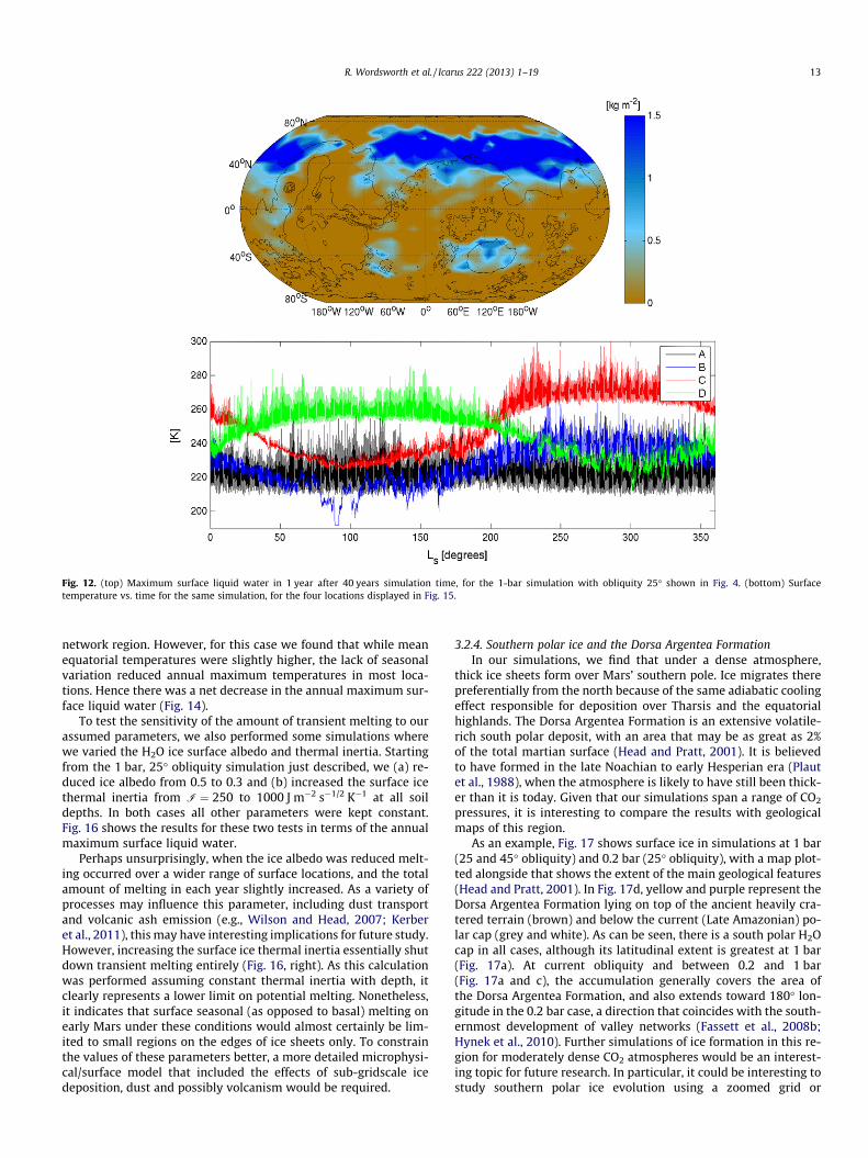
Fig. 12. (top) Maximum surface liquid water in 1 year after 40 years simulation time, for the 1-bar simulation with obliquity 25� shown in Fig. 4. (bottom) Surfacetemperature vs. time for the same simulation, for the four locations displayed in Fig. 15.

R. Wordsworth et al. / Icarus 222 (2013) 1–19 13

network region. However, for this case we found that while meanequatorial temperatures were slightly higher, the lack of seasonalvariation reduced annual maximum temperatures in most loca-tions. Hence there was a net decrease in the annual maximum sur-face liquid water (Fig. 14).

To test the sensitivity of the amount of transient melting to ourassumed parameters, we also performed some simulations wherewe varied the H2O ice surface albedo and thermal inertia. Startingfrom the 1 bar, 25� obliquity simulation just described, we (a) re-duced ice albedo from 0.5 to 0.3 and (b) increased the surface icethermal inertia from I ¼ 250 to 1000 J m�2 s�1/2 K�1 at all soildepths. In both cases all other parameters were kept constant.Fig. 16 shows the results for these two tests in terms of the annualmaximum surface liquid water.

Perhaps unsurprisingly, when the ice albedo was reduced melt-ing occurred over a wider range of surface locations, and the totalamount of melting in each year slightly increased. As a variety ofprocesses may influence this parameter, including dust transportand volcanic ash emission (e.g., Wilson and Head, 2007; Kerberet al., 2011), this may have interesting implications for future study.However, increasing the surface ice thermal inertia essentially shutdown transient melting entirely (Fig. 16, right). As this calculationwas performed assuming constant thermal inertia with depth, itclearly represents a lower limit on potential melting. Nonetheless,it indicates that surface seasonal (as opposed to basal) melting onearly Mars under these conditions would almost certainly be lim-ited to small regions on the edges of ice sheets only. To constrainthe values of these parameters better, a more detailed microphysi-cal/surface model that included the effects of sub-gridscale icedeposition, dust and possibly volcanism would be required.

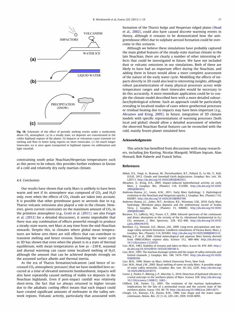
3.2.4. Southern polar ice and the Dorsa Argentea FormationIn our simulations, we find that under a dense atmosphere,

thick ice sheets form over Mars’ southern pole. Ice migrates therepreferentially from the north because of the same adiabatic coolingeffect responsible for deposition over Tharsis and the equatorialhighlands. The Dorsa Argentea Formation is an extensive volatile-rich south polar deposit, with an area that may be as great as 2%of the total martian surface (Head and Pratt, 2001). It is believedto have formed in the late Noachian to early Hesperian era (Plautet al., 1988), when the atmosphere is likely to have still been thick-er than it is today. Given that our simulations span a range of CO2

pressures, it is interesting to compare the results with geologicalmaps of this region.

As an example, Fig. 17 shows surface ice in simulations at 1 bar(25 and 45� obliquity) and 0.2 bar (25� obliquity), with a map plot-ted alongside that shows the extent of the main geological features(Head and Pratt, 2001). In Fig. 17d, yellow and purple represent theDorsa Argentea Formation lying on top of the ancient heavily cra-tered terrain (brown) and below the current (Late Amazonian) po-lar cap (grey and white). As can be seen, there is a south polar H2Ocap in all cases, although its latitudinal extent is greatest at 1 bar(Fig. 17a). At current obliquity and between 0.2 and 1 bar(Fig. 17a and c), the accumulation generally covers the area ofthe Dorsa Argentea Formation, and also extends toward 180� lon-gitude in the 0.2 bar case, a direction that coincides with the south-ernmost development of valley networks (Fassett et al., 2008b;Hynek et al., 2010). Further simulations of ice formation in this re-gion for moderately dense CO2 atmospheres would be an interest-ing topic for future research. In particular, it could be interesting tostudy southern polar ice evolution using a zoomed grid or

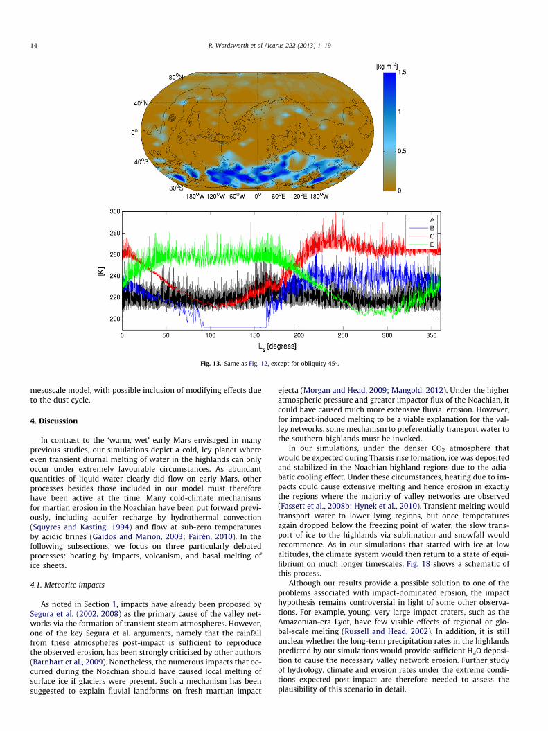
Fig. 13. Same as Fig. 12, except for obliquity 45�.

14 R. Wordsworth et al. / Icarus 222 (2013) 1–19

mesoscale model, with possible inclusion of modifying effects dueto the dust cycle.

4. Discussion

In contrast to the ‘warm, wet’ early Mars envisaged in manyprevious studies, our simulations depict a cold, icy planet whereeven transient diurnal melting of water in the highlands can onlyoccur under extremely favourable circumstances. As abundantquantities of liquid water clearly did flow on early Mars, otherprocesses besides those included in our model must thereforehave been active at the time. Many cold-climate mechanismsfor martian erosion in the Noachian have been put forward previ-ously, including aquifer recharge by hydrothermal convection(Squyres and Kasting, 1994) and flow at sub-zero temperaturesby acidic brines (Gaidos and Marion, 2003; Fairén, 2010). In thefollowing subsections, we focus on three particularly debatedprocesses: heating by impacts, volcanism, and basal melting ofice sheets.

4.1. Meteorite impacts

As noted in Section 1, impacts have already been proposed bySegura et al. (2002, 2008) as the primary cause of the valley net-works via the formation of transient steam atmospheres. However,one of the key Segura et al. arguments, namely that the rainfallfrom these atmospheres post-impact is sufficient to reproducethe observed erosion, has been strongly criticised by other authors(Barnhart et al., 2009). Nonetheless, the numerous impacts that oc-curred during the Noachian should have caused local melting ofsurface ice if glaciers were present. Such a mechanism has beensuggested to explain fluvial landforms on fresh martian impact

ejecta (Morgan and Head, 2009; Mangold, 2012). Under the higheratmospheric pressure and greater impactor flux of the Noachian, itcould have caused much more extensive fluvial erosion. However,for impact-induced melting to be a viable explanation for the val-ley networks, some mechanism to preferentially transport water tothe southern highlands must be invoked.

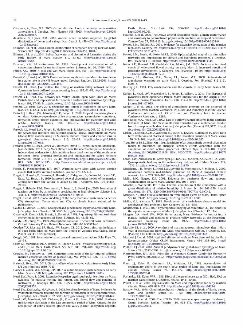
In our simulations, under the denser CO2 atmosphere thatwould be expected during Tharsis rise formation, ice was depositedand stabilized in the Noachian highland regions due to the adia-batic cooling effect. Under these circumstances, heating due to im-pacts could cause extensive melting and hence erosion in exactlythe regions where the majority of valley networks are observed(Fassett et al., 2008b; Hynek et al., 2010). Transient melting wouldtransport water to lower lying regions, but once temperaturesagain dropped below the freezing point of water, the slow trans-port of ice to the highlands via sublimation and snowfall wouldrecommence. As in our simulations that started with ice at lowaltitudes, the climate system would then return to a state of equi-librium on much longer timescales. Fig. 18 shows a schematic ofthis process.

Although our results provide a possible solution to one of theproblems associated with impact-dominated erosion, the impacthypothesis remains controversial in light of some other observa-tions. For example, young, very large impact craters, such as theAmazonian-era Lyot, have few visible effects of regional or glo-bal-scale melting (Russell and Head, 2002). In addition, it is stillunclear whether the long-term precipitation rates in the highlandspredicted by our simulations would provide sufficient H2O deposi-tion to cause the necessary valley network erosion. Further studyof hydrology, climate and erosion rates under the extreme condi-tions expected post-impact are therefore needed to assess theplausibility of this scenario in detail.

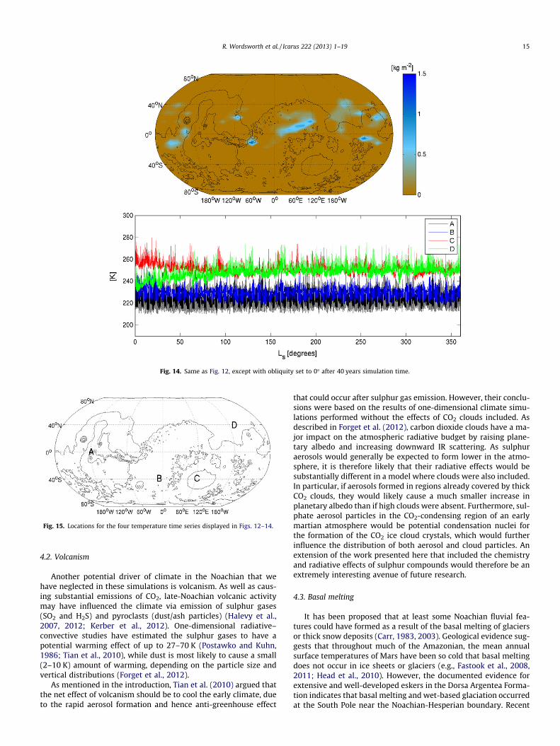
Fig. 14. Same as Fig. 12, except with obliquity set to 0� after 40 years simulation time.

Fig. 15. Locations for the four temperature time series displayed in Figs. 12–14.

R. Wordsworth et al. / Icarus 222 (2013) 1–19 15

4.2. Volcanism

Another potential driver of climate in the Noachian that wehave neglected in these simulations is volcanism. As well as caus-ing substantial emissions of CO2, late-Noachian volcanic activitymay have influenced the climate via emission of sulphur gases(SO2 and H2S) and pyroclasts (dust/ash particles) (Halevy et al.,2007, 2012; Kerber et al., 2012). One-dimensional radiative–convective studies have estimated the sulphur gases to have apotential warming effect of up to 27–70 K (Postawko and Kuhn,1986; Tian et al., 2010), while dust is most likely to cause a small(2–10 K) amount of warming, depending on the particle size andvertical distributions (Forget et al., 2012).

As mentioned in the introduction, Tian et al. (2010) argued thatthe net effect of volcanism should be to cool the early climate, dueto the rapid aerosol formation and hence anti-greenhouse effect

that could occur after sulphur gas emission. However, their conclu-sions were based on the results of one-dimensional climate simu-lations performed without the effects of CO2 clouds included. Asdescribed in Forget et al. (2012), carbon dioxide clouds have a ma-jor impact on the atmospheric radiative budget by raising plane-tary albedo and increasing downward IR scattering. As sulphuraerosols would generally be expected to form lower in the atmo-sphere, it is therefore likely that their radiative effects would besubstantially different in a model where clouds were also included.In particular, if aerosols formed in regions already covered by thickCO2 clouds, they would likely cause a much smaller increase inplanetary albedo than if high clouds were absent. Furthermore, sul-phate aerosol particles in the CO2-condensing region of an earlymartian atmosphere would be potential condensation nuclei forthe formation of the CO2 ice cloud crystals, which would furtherinfluence the distribution of both aerosol and cloud particles. Anextension of the work presented here that included the chemistryand radiative effects of sulphur compounds would therefore be anextremely interesting avenue of future research.

4.3. Basal melting

It has been proposed that at least some Noachian fluvial fea-tures could have formed as a result of the basal melting of glaciersor thick snow deposits (Carr, 1983, 2003). Geological evidence sug-gests that throughout much of the Amazonian, the mean annualsurface temperatures of Mars have been so cold that basal meltingdoes not occur in ice sheets or glaciers (e.g., Fastook et al., 2008,2011; Head et al., 2010). However, the documented evidence forextensive and well-developed eskers in the Dorsa Argentea Forma-tion indicates that basal melting and wet-based glaciation occurredat the South Pole near the Noachian-Hesperian boundary. Recent

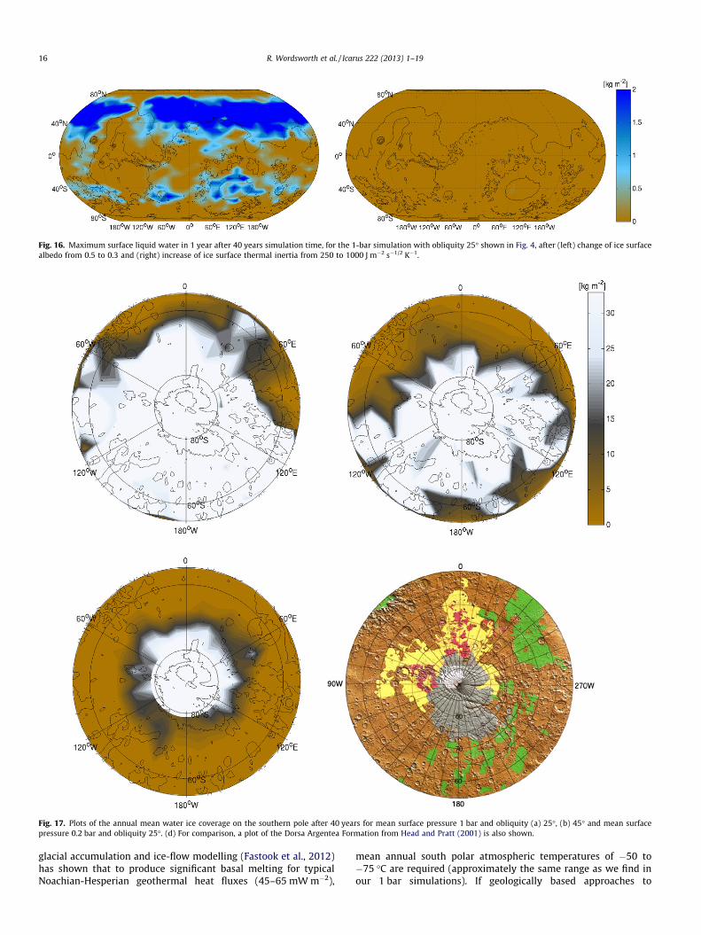
Fig. 16. Maximum surface liquid water in 1 year after 40 years simulation time, for the 1-bar simulation with obliquity 25� shown in Fig. 4, after (left) change of ice surfacealbedo from 0.5 to 0.3 and (right) increase of ice surface thermal inertia from 250 to 1000 J m�2 s�1/2 K�1.

Fig. 17. Plots of the annual mean water ice coverage on the southern pole after 40 years for mean surface pressure 1 bar and obliquity (a) 25�, (b) 45� and mean surfacepressure 0.2 bar and obliquity 25�. (d) For comparison, a plot of the Dorsa Argentea Formation from Head and Pratt (2001) is also shown.

16 R. Wordsworth et al. / Icarus 222 (2013) 1–19

glacial accumulation and ice-flow modelling (Fastook et al., 2012)has shown that to produce significant basal melting for typicalNoachian-Hesperian geothermal heat fluxes (45–65 mW m�2),

mean annual south polar atmospheric temperatures of �50 to�75 �C are required (approximately the same range as we find inour 1 bar simulations). If geologically based approaches to

LIQUID WATER

PRECIPITATION(SNOW)

VOLCANISM

WATER ICE

IMPACTORS

(a)

(b)

(c)Fig. 18. Schematic of the effect of periodic melting events under a moderatelydense CO2 atmosphere. (a) In a steady state, ice deposits are concentrated in thecolder highland regions of the planet. (b) Impacts or volcanism cause transient icemelting and flow to lower lying regions on short timescales. (c) On much longertimescales, ice is once again transported to highland regions via sublimation andlight snowfall.

R. Wordsworth et al. / Icarus 222 (2013) 1–19 17

constraining south polar Noachian/Hesperian temperatures suchas this prove to be robust, this provides further evidence in favourof a cold and relatively dry early martian climate.

4.4. Conclusions

Our results have shown that early Mars is unlikely to have beenwarm and wet if its atmosphere was composed of CO2 and H2Oonly, even when the effects of CO2 clouds are taken into account.It is possible that other greenhouse gases or aerosols due to e.g.Tharsis volcanic emissions also played a role in the climate. How-ever, given current constraints on the maximum amount of CO2 inthe primitive atmosphere (e.g., Grott et al. (2011); see also Forgetet al. (2012) for a detailed discussion), it seems improbable thatthere was any combination of effects powerful enough to producea steady-state warm, wet Mars at any time from the mid-Noachianonwards. Despite this, in climates where global mean tempera-tures are below zero there are still effects that can contribute totransient melting and hence erosion. Simulating the water cyclein 3D has shown that even when the planet is in a state of thermalequilibrium, with mean temperatures as low as �230 K, seasonaland diurnal warming can cause some localised melting of H2O,although the amount that can be achieved depends strongly onthe assumed surface albedo and thermal inertia.

As the era of Tharsis formation/volcanism (and hence of in-creased CO2 atmospheric pressure) that we have modelled here oc-curred at a time of elevated meteorite bombardment, impacts willalso have repeatedly caused melting of stable ice deposits in theNoachian highlands. Even if post-impact rainfall was relativelyshort-term, the fact that ice always returned to higher terraindue to the adiabatic cooling effect means that each impact couldhave created significant amounts of meltwater in the valley net-work regions. Volcanic activity, particularly that associated with

formation of the Tharsis bulge and Hesperian ridged plains (Headet al., 2002), could also have caused discrete warming events intheory, although it remains to be demonstrated how the anti-greenhouse effect due to sulphate aerosol formation could be over-come in this scenario.

Although we believe these simulations have probably capturedthe main global features of the steady-state martian climate in thelate Noachian, there are clearly a number of other interesting ef-fects that could be investigated in future. We have not includeddust or volcanic emissions in our simulations. Both of these arelikely to have had an important effect during the Noachian, andadding them in future would allow a more complete assessmentof the nature of the early water cycle. Modelling the effects of im-pacts directly in 3D could also lead to interesting insights, althoughrobust parameterization of many physical processes across widetemperature ranges and short timescales would be necessary todo this accurately. A more immediate application could be to cou-ple the climate model described here with a more detailed subsur-face/hydrological scheme. Such an approach could be particularlyrevealing in localised studies of cases where geothermal processesor residual heating due to impacts may have been important (e.g.,Abramov and Kring, 2005). In future, integration of 3D climatemodels with specific representations of warming processes (bothlocal and global) should allow a detailed assessment of whetherthe observed Noachian fluvial features can be reconciled with thecold, mainly frozen planet simulated here.

Acknowledgments

This article has benefited from discussions with many research-ers, including Jim Kasting, Nicolas Mangold, William Ingram, AlanHoward, Bob Haberle and Franck Selsis.

References

Abbot, D.S., Voigt, A., Branson, M., Pierrehumbert, R.T., Pollard, D., Le Hir, V., Koll,D.D.B., 2012. Clouds and Snowball Earth deglaciation. Geophys. Res. Lett. 39,L20711. http://dx.doi.org/10.1029/2005JE002453.

Abramov, O., Kring, D.A., 2005. Impact-induced hydrothermal activity on earlyMars. J. Geophys. Res. (Planets) 110, E12S09. http://dx.doi.org/10.1029/2005JE002453.

Andrews-Hanna, J.C., Lewis, K.W., 2011. Early Mars hydrology: 2. Hydrologicalevolution in the Noachian and Hesperian epochs. J. Geophys. Res. (Planets) 116,E02007. http://dx.doi.org/10.1029/2010JE003709.

Andrews-Hanna, J.C., Zuber, M.T., Arvidson, R.E., Wiseman, S.M., 2010. Early Marshydrology: Meridiani playa deposits and the sedimentary record of ArabiaTerra. J. Geophys. Res. (Planets) 15, E06002. http://dx.doi.org/10.1029/2009JE003485.

Baranov, Y.I., Lafferty, W.J., Fraser, G.T., 2004. Infrared spectrum of the continuumand dimer absorption in the vicinity of the O2 vibrational fundamental in O2/CO2 mixtures. J. Mol. Spectrosc. 228, 432–440. http://dx.doi.org/10.1016/j.jms.2004.04.010.

Barnhart, C.J., Howard, A.D., Moore, J.M., 2009. Long-term precipitation and late-stage valley network formation: Landform simulations of Parana Basin, Mars. J.Geophys. Res. (Planets) 114, E01003. http://dx.doi.org/10.1029/2008JE003122.

Bibring, J.-P. et al., 2006. Global mineralogical and aqueous Mars history derivedfrom OMEGA/Mars express data. Science 312, 400–404. http://dx.doi.org/10.1126/science.1122659.

Carr, M.H., 1983. Stability of streams and lakes on Mars. Icarus 56, 476–495. http://dx.doi.org/10.1016/0019-1035(83)90168-9.

Carr, M.H., 1995. The martian drainage system and the origin of valley networks andfretted channels. J. Geophys. Res. 100, 7479–7507. http://dx.doi.org/10.1029/95JE00260.

Carr, M.H., 1996. Water on Mars. Oxford University Press, New York.Carr, M.H., Head, J.W., 2003. Basal melting of snow on early Mars: A possible origin

of some valley networks. Geophys. Res. Lett. 30 (24), 2245. http://dx.doi.org/10.1029/2003GL018575.

Carter, J., Poulet, F., Bibring, J.-P., Murchie, S., 2010. Detection of hydrated silicates incrustal outcrops in the northern plains of Mars. Science 328. http://dx.doi.org/10.1126/science.1189013, 1682–.

Clifford, S.M., Parker, T.J., 2001. The evolution of the martian hydrosphere:Implications for the fate of a primordial ocean and the current state of thenorthern plains. Icarus 154, 40–79. http://dx.doi.org/10.1006/icar.2001.6671.

Clough, S.A., Kneizys, F.X., Davies, R.W., 1989. Line shape and the water vaporcontinuum. Atmos. Res. 23 (3–4), 229–241, ISSN: 0169-8095.

18 R. Wordsworth et al. / Icarus 222 (2013) 1–19

Colaprete, A., Toon, O.B., 2003. Carbon dioxide clouds in an early dense martianatmosphere. J. Geophys. Res. (Planets) 108, 5025. http://dx.doi.org/10.1029/2002JE001967.

di Achille, G., Hynek, B.M., 2010. Ancient ocean on Mars supported by globaldistribution of deltas and valleys. Nat. Geosci. 3, 459–463. http://dx.doi.org/10.1038/ngeo891.

Ehlmann, B.L. et al., 2008. Orbital identification of carbonate-bearing rocks on Mars.Science 322. http://dx.doi.org/10.1126/science.1164759, 1828–.

Ehlmann, B.L. et al., 2011. Subsurface water and clay mineral formation during theearly history of Mars. Nature 479, 53–60. http://dx.doi.org/10.1038/nature10582.

Emanuel, K.A., Ivkovi-Rothman, M., 1999. Development and evaluation of aconvection scheme for use in climate models. J. Atmos. Sci. 56, 1766–1782.

Fairén, A.G., 2010. A cold and wet Mars. Icarus 208, 165–175. http://dx.doi.org/10.1016/j.icarus.2010.01.006.

Fassett, C.I., Head, J.W., 2005. Fluvial sedimentary deposits on Mars: Ancient deltasin a crater lake in the Nili Fossae region. Geophys. Res. Lett. 32, L14201. http://dx.doi.org/10.1029/2005GL023456.

Fassett, C.I., Head, J.W., 2008a. The timing of martian valley network activity:Constraints from buffered crater counting. Icarus 195, 61–89. http://dx.doi.org/10.1016/j.icarus.2007.12.009.

Fassett, C.I., Head, J.W., network-fed, Valley, 2008b. open-basin lakes on Mars:Distribution and implications for Noachian surface and subsurface hydrology.Icarus 198, 37–56. http://dx.doi.org/10.1016/j.icarus.2008.06.016.

Fassett, C.I., Head, J.W., 2011. Sequence and timing of conditions on early Mars.Icarus 211, 1204–1214. http://dx.doi.org/10.1016/j.icarus.2010.11.014.

Fastook, J.L., Head, J.W., Marchant, D.R., Forget, F., 2008. Tropical mountain glacierson Mars: Altitude-dependence of ice accumulation, accumulation conditions,formation times, glacier dynamics, and implications for planetary spin-axis/orbital history. Icarus 198, 305–317. http://dx.doi.org/10.1016/j.icarus.2008.08.008.

Fastook, J.L., Head, J.W., Forget, F., Madeleine, J.-B., Marchant, D.R., 2011. Evidencefor Amazonian northern mid-latitude regional glacial landsystems on Mars:Glacial flow models using GCM-driven climate results and comparisons togeological observations. Icarus 216, 23–39. http://dx.doi.org/10.1016/j.icarus.2011.07.018.

Fastook, James L., Head, James W., Marchant, David R., Forget, Francois, Madeleine,Jean-Baptiste, 2012. Early Mars climate near the noachianhesperian boundary:Independent evidence for cold conditions from basal melting of the south polarice sheet (dorsa argentea formation) and implications for valley networkformation. Icarus 219 (1), 25–40. http://dx.doi.org/10.1016/j.icarus.2012.02.013, ISSN: 0019-1035. <http://www.sciencedirect.com/science/article/pii/S0019103512000619>.

Forget, F., Pierrehumbert, R.T., 1997. Warming early Mars with carbon dioxideclouds that scatter infrared radiation. Science 278, 1273–+.

Forget, F., Hourdin, F., Fournier, R., Hourdin, C., Talagrand, O., Collins, M., Lewis, S.R.,Read, P.L., Huot, J.-P., 1999. Improved general circulation models of the martianatmosphere from the surface to above 80 km. J. Geophys. Res. 104, 24155–24176.

Forget, F., Haberle, R.M., Montmessin, F., Levrard, B., Head, J.W., 2006. Formation ofglaciers on Mars by atmospheric precipitation at high obliquity. Science 311,368–371. http://dx.doi.org/10.1126/science.1120335.

Forget, F. et al., 2012. Global modeling of the early martian climate under a denserCO2 atmosphere: Temperature and CO2 ice clouds. Icarus, submitted forpublication.

Gaidos, E., Marion, G., 2003. Geological and geochemical legacy of a cold early Mars.J. Geophys. Res. (Planets) 108, 5055. http://dx.doi.org/10.1029/2002JE002000.

Galperin, B., Kantha, L.H., Hassid, S., Rosati, A., 1988. A quasi-equilibrium turbulentenergy model for geophysical flows. J. Atmos. Sci. 45, 55–62.

Goody, R.M., Yung, Y.L., 1989. Atmospheric Radiation: Theoretical Basis, second ed.Oxford University Press, Oxford, New York. ISBN 0-19-505134-3.

Goudge, T.A., Mustard, J.F., Head, J.W., Fassett, C.I., 2012. Constraints on the historyof open-basin lakes on Mars from the timing of volcanic resurfacing. LunarPlanet. Sci. 43, 1328 (abstract).

Gough, D.O., 1981. Solar interior structure and luminosity variations. Solar Phys. 74,21–34.

Grott, M., Morschhauser, A., Breuer, D., Hauber, E., 2011. Volcanic outgassing of CO2

and H2O on Mars. Earth Planet. Sci. Lett. 308, 391–400. http://dx.doi.org/10.1016/j.epsl.2011.06.014.

Gruszka, M., Borysow, A., 1998. Computer simulation of the far infrared collisioninduced absorption spectra of gaseous CO2. Mol. Phys. 93, 1007–1016. http://dx.doi.org/10.1080/002689798168709.

Halevy, I., Head, J.W., 2012. Climatic effects of punctuated volcanism on early Mars.LPI Contributions 1680, 7043.

Halevy, I., Zuber, M.T., Schrag, D.P., 2007. A sulfur dioxide climate feedback on earlyMars. Science 318. http://dx.doi.org/10.1126/science.1147039, 1903–.

Head, J.W., Pratt, S., 2001. Extensive Hesperian-aged south polar ice sheet on Mars:Evidence for massive melting and retreat, and lateral flow and ponding ofmeltwater. J. Geophys. Res. 106, 12275–12300. http://dx.doi.org/10.1029/2000JE001359.

Head, J.W., Kreslavsky, M.A., Pratt, S., 2002. Northern lowlands of Mars: Evidence forwidespread volcanic flooding and tectonic deformation in the Hesperian Period.J. Geophys. Res. (Planets) 107, 5003. http://dx.doi.org/10.1029/2000JE001445.

Head, J.W., Marchant, D.R., Dickson, J.L., Kress, A.M., Baker, D.M., 2010. Northernmid-latitude glaciation in the Late Amazonian period of Mars: Criteria for therecognition of debris-covered glacier and valley glacier landsystem deposits.

Earth Planet. Sci. Lett. 294, 306–320. http://dx.doi.org/10.1016/j.epsl.2009.06.041.

Hourdin, F. et al., 2006. The LMDZ4 general circulation model: Climate performanceand sensitivity to parametrized physics with emphasis on tropical convection.Climate Dyn. 27, 787–813. http://dx.doi.org/10.1007/s00382-006-0158-0.

Hynek, B.M., Phillips, R.J., 2001. Evidence for extensive denudation of the martianhighlands. Geology 29. http://dx.doi.org/10.1130/0091-7613(2001)029<0407:EFEDOT>2.0.CO;2, 407–+.

Hynek, B.M., Beach, M., Hoke, M.R.T., 2010. Updated global map of martian valleynetworks and implications for climate and hydrologic processes. J. Geophys.Res. (Planets) 115, E09008. http://dx.doi.org/10.1029/2009JE003548.

Irwin, R.P., Howard, A.D., Craddock, R.A., Moore, J.M., 2005. An intense terminalepoch of widespread fluvial activity on early Mars: 2. Increased runoff andpaleolake development. J. Geophys. Res. (Planets) 110 (9). http://dx.doi.org/10.1029/2005JE002460, 12–+.

Johnson, S.S., Mischna, M.A., Grove, T.L., Zuber, M.T., 2008. Sulfur-inducedgreenhouse warming on early Mars. J. Geophys. Res. (Planets) 113 (12),8005–+.

Kasting, J.F., 1991. CO2 condensation and the climate of early Mars. Icarus 94,1–13.

Kerber, L., Head, J.W., Madeleine, J.-B., Forget, F., Wilson, L., 2011. The dispersal ofpyroclasts from Apollinaris Patera, Mars: Implications for the origin of theMedusae Fossae Formation. Icarus 216, 212–220. http://dx.doi.org/10.1016/j.icarus.2011.07.035.

Kerber, L. et al., 2012. The effect of atmospheric pressure on the dispersal ofpyroclasts from martian volcanoes. In: Lunar and Planetary Institute ScienceConference Abstracts, vol. 43 of Lunar and Planetary Institute ScienceConference Abstracts, p. 1295.

Kreslavsky, M.A., Head, J.W., 2002. Fate of outflow channel effluents in the northernlowlands of Mars: The Vastitas Borealis Formation as a sublimation residuefrom frozen ponded bodies of water. J. Geophys. Res. (Planets) 107, 5121. http://dx.doi.org/10.1029/2001JE001831.

Laskar, J., Correia, A.C.M., Gastineau, M., Joutel, F., Levrard, B., Robutel, P., 2004. Longterm evolution and chaotic diffusion of the insolation quantities of Mars. Icarus170, 343–364. http://dx.doi.org/10.1016/j.icarus.2004.04.005.

Treut, Hervé Le, Li, Zhao-Xin, 1991. Sensitivity of an atmospheric general circulationmodel to prescribed sst changes: Feedback effects associated with thesimulation of cloud optical properties. Climate Dyn. 5, 175–187. http://dx.doi.org/10.1007/BF00251808, ISSN: 0930-7575. http://dx.doi.org/10.1007/BF00251808.

Lewis, K.W., Aharonson, O., Grotzinger, J.P., Kirk, R.L., McEwen, A.S., Suer, T.-A., 2008.Quasi-periodic bedding in the sedimentary rock record of Mars. Science 322,1532. http://dx.doi.org/10.1126/science.1161870.

Madeleine, J.-B., Forget, F., Head, J.W., Levrard, B., Montmessin, F., Millour, E., 2009.Amazonian northern mid-latitude glaciation on Mars: A proposed climatescenario. Icarus 203, 390–405. http://dx.doi.org/10.1016/j.icarus.2009.04.037.

Malin, M.C., Edgett, K.S., 2003. Evidence for persistent flow and aqueoussedimentation on early Mars. Science 302, 1931–1934.

Manabe, S., Wetherald, R.T., 1967. Thermal equilibrium of the atmosphere with agiven distribution of relative humidity. J. Atmos. Sci. 24, 241–259. http://dx.doi.org/10.1175/1520-0469(1967)024<0241:TEOTAW>2.0.CO;2.

Mangold, N., 2012. Fluvial landforms on fresh impact ejecta on Mars. Planet. SpaceSci. 62, 69–85. http://dx.doi.org/10.1016/j.pss.2011.12.009.

Mellor, G.L., Yamada, T., 1982. Development of a turbulence closure model forgeophysical fluid problems. Rev. Geophys. 20, 851–875.

Montmessin, F. et al., 2007. Hyperspectral imaging of convective CO2 ice clouds inthe equatorial mesosphere of Mars. J. Geophys. Res. (Planets) 112, 11–+.

Morgan, G.A., Head, J.W., 2009. Sinton crater, Mars: Evidence for impact into aplateau icefield and melting to produce valley networks at the Hesperian-Amazonian boundary. Icarus 202, 39–59. http://dx.doi.org/10.1016/j.icarus.2009.02.025.

Murchie, S.L. et al., 2009. A synthesis of martian aqueous mineralogy after 1 Marsyear of observations from the Mars Reconnaissance Orbiter. J. Geophys. Res.(Planets) 114, E00D06. http://dx.doi.org/10.1029/2009JE003342.

Mustard, J.F. et al., 2008. Hydrated silicate minerals on Mars observed by the MarsReconnaissance Orbiter CRISM instrument. Nature 454, 305–309. http://dx.doi.org/10.1038/nature07097.

Phillips, R.J. et al., 2001. Ancient geodynamics and global-scale hydrology on Mars.Science 291, 2587–2591. http://dx.doi.org/10.1126/science.1058701.

Pierrehumbert, R.T., 2011. Principles of Planetary Climate. Cambridge UniversityPress, ISBN: 9780521865562. <http://books.google.com/books?id=bO_U8f5pVR8C>.

Plaut, J.J., Kahn, R., Guinness, E.A., Arvidson, R.E., 1988. Accumulation ofsedimentary debris in the south polar region of Mars and implications forclimate history. Icarus 76, 357–377. http://dx.doi.org/10.1016/0019-1035(88)90076-0.

Postawko, S.E., Kuhn, W.R., 1986. Effect of the greenhouse gases (CO2, H2O, SO2) onmartian paleoclimate. J. Geophys. Res. 91, D431–D438.

Poulet, F. et al., 2005. Phyllosilicates on Mars and implications for early martianclimate. Nature 438, 623–627. http://dx.doi.org/10.1038/nature04274.

Rossow, W.B., 1978. Cloud microphysics – Analysis of the clouds of Earth, Venus,Mars, and Jupiter. Icarus 36, 1–50. http://dx.doi.org/10.1016/0019-1035(78)90072-6.

Rothman, L.S. et al., 2009. The HITRAN 2008 molecular spectroscopic database. J.Quant. Spectros. Radiat. Transfer 110, 533–572. http://dx.doi.org/10.1016/j.jqsrt.2009.02.013.

R. Wordsworth et al. / Icarus 222 (2013) 1–19 19

Russell, P.S., Head, J.W., 2002. The martian hydrosphere/cryosphere system:Implications of the absence of hydrologic activity at Lyot crater. Geophys. Res.Lett. 29 (17), 1827. http://dx.doi.org/10.1029/2002GL015178.

Sadourny, R., 1975. The dynamics of finite-difference models of the shallow-waterequations. J. Atmos. Sci. 32, 680–689.

Salvatore, M.R., Mustard, J.F., Wyatt, M.B., Murchie, S.L., 2010. Definitive evidence ofHesperian basalt in Acidalia and Chryse planitiae. J. Geophys. Res. (Planets) 115,E07005. http://dx.doi.org/10.1029/2009JE003519.

Segura, T.L., Toon, O.B., Colaprete, A., Zahnle, K., 2002. Environmental effects of largeimpacts on Mars. Science 298, 1977–1980.

Segura, T.L., Toon, O.B., Colaprete, A., 2008. Modeling the environmental effects ofmoderate-sized impacts on Mars. J. Geophys. Res. (Planets) 113, E11007. http://dx.doi.org/10.1029/2008JE003147.

Selsis, F., Wordsworth, R.D., Forget, F., 2011. Thermal phase curves of nontransitingterrestrial exoplanets. I. Characterizing atmospheres. Astron. Astrophys. 532,A1+. http://dx.doi.org/10.1051/0004-6361/201116654.

Squyres, S.W., Kasting, J.F., 1994. Early Mars: How warm and how wet? Science 265,744–749. http://dx.doi.org/10.1126/science.265.5173.744.

Tian, F. et al., 2010. Photochemical and climate consequences of sulfur outgassingon early Mars. Earth Planet. Sci. Lett. 295, 412–418. http://dx.doi.org/10.1016/j.epsl.2010.04.016.

Toon, O.B., McKay, C.P., Ackerman, T.P., Santhanam, K., 1989. Rapid calculation ofradiative heating rates and photodissociation rates in inhomogeneous multiplescattering atmospheres. J. Geophys. Res. 94, 16287–16301.

Toon, O.B., Segura, T., Zahnle, K., 2010. The formation of martian river valleys byimpacts. Annu. Rev. Earth Planet. Sci. 38, 303–322. http://dx.doi.org/10.1146/annurev-earth-040809-152354.

Wilson, L., Head, J.W., 2007. Explosive volcanic eruptions on Mars: Tephra andaccretionary lapilli formation, dispersal and recognition in the geologic record.J. Volcanol. Geotherm. Res. 163, 83–97. http://dx.doi.org/10.1016/j.jvolgeores.2007.03.007.

Wordsworth, R., Forget, F., Eymet, V., 2010a. Infrared collision-induced and far-lineabsorption in dense CO2 atmospheres. Icarus 210, 992–997. http://dx.doi.org/10.1016/j.icarus.2010.06.010.

Wordsworth, R., Forget, F., Selsis, F., Madeleine, J.-B., Millour, E., Eymet, V., 2010b. IsGliese 581d habitable? Some constraints from radiative–convective climatemodeling. Astron. Astrophys. 522, A22+. http://dx.doi.org/10.1051/0004-6361/201015053.

Wordsworth, R.D., Forget, F., Selsis, F., Millour, E., Charnay, B., Madeleine, J.-B., 2011.Gliese 581d is the first discovered terrestrial-mass exoplanet in the habitablezone. Astrophys. J. Lett. 733, L48+. http://dx.doi.org/10.1088/2041-8205/733/2/L48.