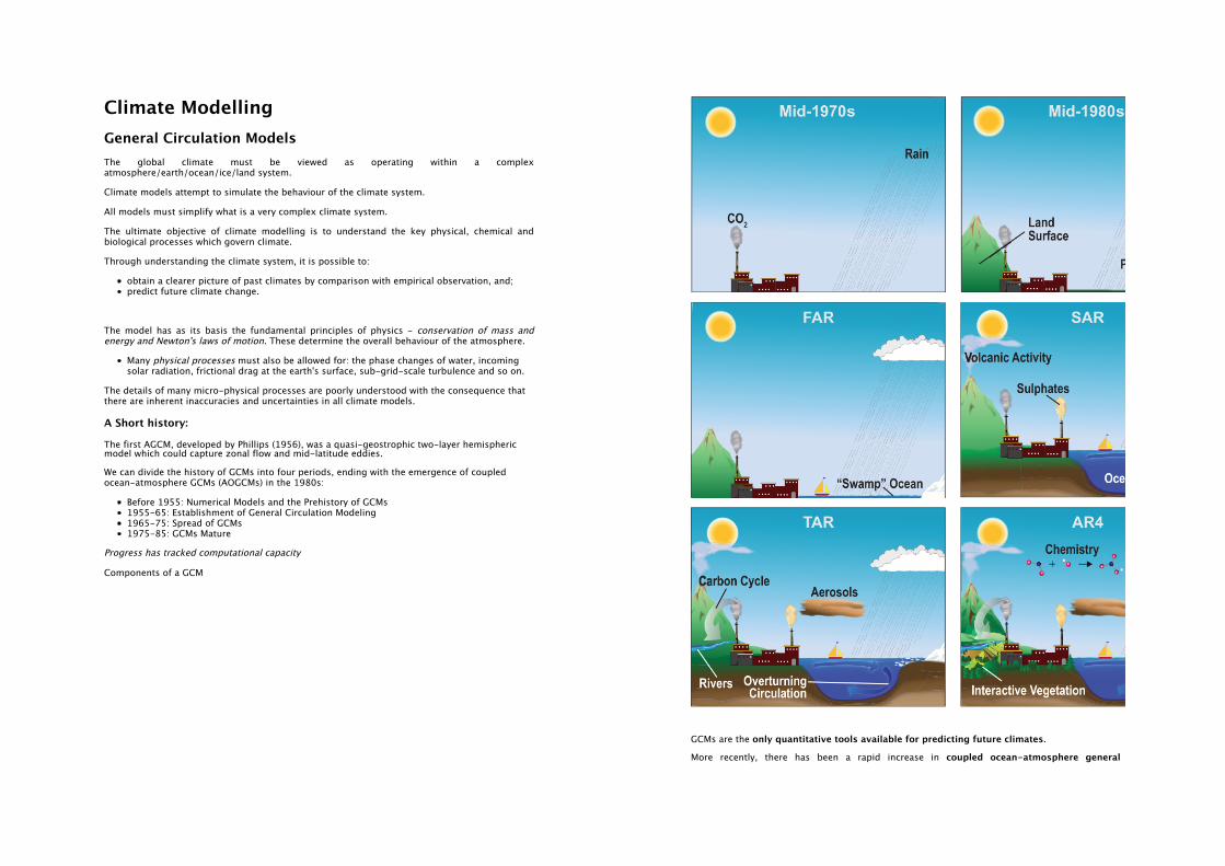
Climate Modelling

General Circulation Models

The global climate must be viewed as operating within a complexatmosphere/earth/ocean/ice/land system.

Climate models attempt to simulate the behaviour of the climate system.

All models must simplify what is a very complex climate system.

The ultimate objective of climate modelling is to understand the key physical, chemical andbiological processes which govern climate.

Through understanding the climate system, it is possible to:

obtain a clearer picture of past climates by comparison with empirical observation, and; predict future climate change.

The model has as its basis the fundamental principles of physics - conservation of mass andenergy and Newton's laws of motion. These determine the overall behaviour of the atmosphere.

Many physical processes must also be allowed for: the phase changes of water, incomingsolar radiation, frictional drag at the earth's surface, sub-grid-scale turbulence and so on.

The details of many micro-physical processes are poorly understood with the consequence thatthere are inherent inaccuracies and uncertainties in all climate models.

A Short history:

The first AGCM, developed by Phillips (1956), was a quasi-geostrophic two-layer hemisphericmodel which could capture zonal flow and mid-latitude eddies.

We can divide the history of GCMs into four periods, ending with the emergence of coupledocean-atmosphere GCMs (AOGCMs) in the 1980s:

Before 1955: Numerical Models and the Prehistory of GCMs1955-65: Establishment of General Circulation Modeling1965-75: Spread of GCMs1975-85: GCMs Mature

Progress has tracked computational capacity

Components of a GCM

GCMs are the only quantitative tools available for predicting future climates.

More recently, there has been a rapid increase in coupled ocean-atmosphere general

circulation models (AOGCMs).

These are the most complex type of model and is difficult to model accurately.

The development of more accurate coupled models has been a primary focus for some time,since it is more generally accepted that it is through these models that we can get a scientificunderstanding of climate and climate change.

What does a GCM do?

AOGCMs represent the most sophisticated attempt to simulate the earth system.

There are three major sets of processes which must be considered when constructing a climatemodel:1) radiative processes- the transfer of radiation through the climate system (e.g. absorption,reflection); radiation drives the system!

2) dynamic processes - the horizontal and vertical transfer of energy (e.g. advection,convection, diffusion);

3) surface process - inclusion of processes involving land/ocean/ice, and the effects of albedo,emissivity and surface-atmosphere energy exchanges.

These are the processes fundamental to the behaviour of the global climate system.

From http://www.acad.carleton.edu/curricular/GEOL/DaveSTELLA/climate/climate_modeling_1.htm

An AOGCM must then take into account all the components that affect global climate:

1. Processes in the Atmosphere:

RadiationAerosolsClouds

ConvectionPrecipitation - large-scale and convectiveBoundary-layer

2. Processes over Land

Vegetation - like a resistor to water lossSoil moisture - moisture and energy storageAlbedoEnergy partitioning - latent, sensible, storageHydrology

3. Processes in the Ocean

Absorption of radiationSalinity variationCurrentsFreezing/thawing near sea ice boundary

4. Sea Ice processes

Transport of sea iceAlbedo differencesFreezing/thawing near ocean boundary

The Earth’s climate results from interactions all these processes.

(Think of the scales involved in space and time for the components shown here and below.)

For this reason, computer models have been developed which try to mathematically simulate theclimate, including the interaction between the component systems.

The basic laws and other relationships necessary to model the climate system are expressedas a series of equations. Solving these equations --> model output.

How does the GCM work?

In solving the equations it is important to consider the model resolution, in both time andspace. This determines how computationally expensive (storage and CPU time) the model is.

the time step of the model.....how often the model solves the equations in space the horizontal/vertical resolutionthe spatial resolution determines the temporal......higher spatial --> higher temporal --->more computer time.

The globe is broken up into a grid. The grid size reflects the horizontal resolution of the model(eg 250 x 200 km grid).

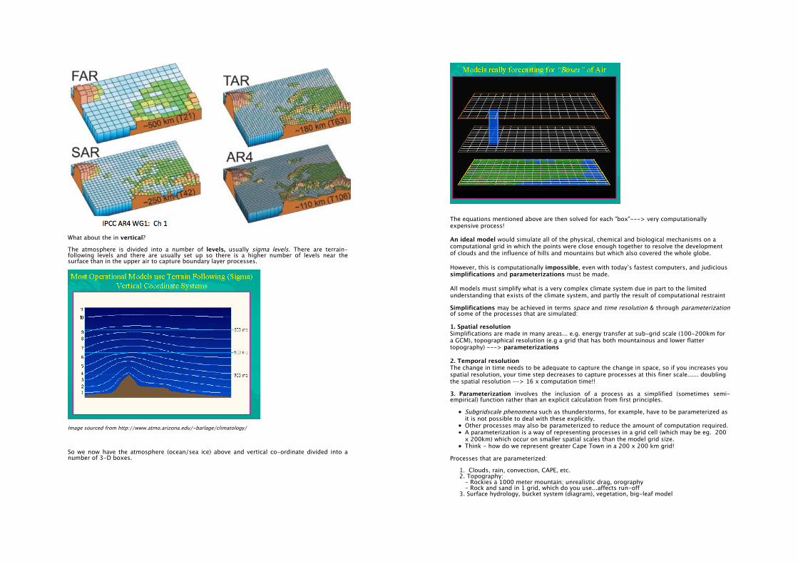
What about the in vertical? The atmosphere is divided into a number of levels, usually sigma levels. There are terrain-following levels and there are usually set up so there is a higher number of levels near thesurface than in the upper air to capture boundary layer processes.

Image sourced from http://www.atmo.arizona.edu/~barlage/climatology/

So we now have the atmosphere (ocean/sea ice) above and vertical co-ordinate divided into anumber of 3-D boxes.

The equations mentioned above are then solved for each "box"---> very computationallyexpensive process!

An ideal model would simulate all of the physical, chemical and biological mechanisms on acomputational grid in which the points were close enough together to resolve the developmentof clouds and the influence of hills and mountains but which also covered the whole globe.

However, this is computationally impossible, even with today’s fastest computers, and judicioussimplifications and parameterizations must be made.

All models must simplify what is a very complex climate system due in part to the limitedunderstanding that exists of the climate system, and partly the result of computational restraint

Simplifications may be achieved in terms space and time resolution & through parameterizationof some of the processes that are simulated:

1. Spatial resolutionSimplifications are made in many areas... e.g. energy transfer at sub-grid scale (100-200km fora GCM), topographical resolution (e.g a grid that has both mountainous and lower flattertopography) ---> parameterizations

2. Temporal resolutionThe change in time needs to be adequate to capture the change in space, so if you increases youspatial resolution, your time step decreases to capture processes at this finer scale...... doublingthe spatial resolution --> 16 x computation time!!

3. Parameterization involves the inclusion of a process as a simplified (sometimes semi-empirical) function rather than an explicit calculation from first principles.

Subgridscale phenomena such as thunderstorms, for example, have to be parameterized asit is not possible to deal with these explicitly. Other processes may also be parameterized to reduce the amount of computation required. A parameterization is a way of representing processes in a grid cell (which may be eg. 200x 200km) which occur on smaller spatial scales than the model grid size. Think - how do we represent greater Cape Town in a 200 x 200 km grid!

Processes that are parameterized:

1. Clouds, rain, convection, CAPE, etc. 2. Topography: - Rockies a 1000 meter mountain; unrealistic drag, orography - Rock and sand in 1 grid, which do you use...affects run-off 3. Surface hydrology, bucket system (diagram), vegetation, big-leaf model

- but plants are varied (deeper roots, greater canopy) so work with functional types: : canopy heights, albedo, leaf area index, transpiration rate, roughness length,seasonality : usually can have 2 types per grid cell.

4. Boundary layer - energy transfer and dissipation (through turbulence)

5. Ice - multi year albedos, ice transport, ice-atm interactions

To produce simulations for many years (5, 15, 50, 150 years), these simplifications need to bemade.

Despite these compromises, GCMs are vital in broadening understanding of key physical,chemical and biological processes which govern climate as well as future climate.

Applications:

Sensitivity studies: model sensitivity of global system to perturbations. Data Assimilation - Generate gridded products for users and to initialize forecast models - Seasonal forecasting - Climate change in response to changes in atmospheric chemistry (eg CO2 effects) - Paleo-climates

However, regional climate is often affected by forcings and circulations that occur at thesub-AOGCM horizontal grid scale.

1. Thus, AOGCMs are not able to provide a detailed description of current climate (or detailedprojections of likely climate change) on space scales smaller than the horizontal resolution,

2. Nor can they explicitly capture the fine scale structure that characterizes climatic variablesin many regions of the world.

For example:

In order to capture these finer scale features, GCMs would have needed to be run at much higher

resolutions.

This, however, is impractical as computational cost becomes too high. A doubling of resolutionresults in an eight-fold increase in computational cost.

How to go from GCM resolution to finer regional scale of impact???

Producing data at the regional scale - Downscaling

We downscale low resolution data to a higher resolution using two downscaling techniques:

Numerical/DynamicalDownscaling

Global Climate ModelResolution

Statistical/Empirical Downscaling

Data from the GCM is usedby Regional Climate Models(RCMs) to numericallysimulate the climatecharacteristics at a muchhigher resolution.

Results in a griddedproduct.

Statistical relationships betweenweather stations on the ground andatmospheric circulations areestablished.

GCM-produced atmosphericcirculations can then be downscaledto the station scale.

Downscaling is used in many different applications:

paleoclimates studiesmodeling present day climate characteristicspossible future climate statesresearch tools to advance the understanding of regional-scale processeshelp develop parameterizations of these processes for use in large scale weather forecastand climate prediction models.many other applications....

Regional climate modelling provides the means to simulate/model circulation at a regional scaledown to very high resolutions.

So using GCM data, downscaling methods provided data at the regional, more useful (?) scale.

BUT, a downscaled product is only as good as its forcing GCM data!

Shortcomings of climate models

Most noticeably that need to simplify the natural system to problems a computer can work with(resolution), Many aspects of the system that are not well understood (physics and parameterizations).

The IPCC lists some short comings:

Discrepancies exist between the vertical profile of temperature change in the troposphereseen in observations and those predicted models.Large uncertainties in estimates of internal climate variability (also referred to as naturalclimate variability) from models and observations. Considerable uncertainty in the reconstructions of solar and volcanic forcing which arebased on limited observational data for all but the last two decades. Large uncertainties in anthropogenic forcings associated with the effects of aerosols.

The roles of clouds and ocean currents in the climate systemThe sensitivity of the climate system to changes in greenhouse gas concentrationsLarge differences in the response of different models to the same forcing

Future anthropogenic factors are also difficult to model:"Future human contributions to climate forcing and potential environmental changeswill depend on the rates and levels of population change, economic growth,development and diffusion of technologies, and other dynamics in human systems. These developments are unpredictable over the long timescales relevant for climatechange research."Storylines.....

Future solar radiationSolar radiation is the source of energy in the climate system; Changes in the intensity of solar radiation will affect global climate We currently do not know how to forecast future changes in solar intensity.

Although climate models have shortcomings, they are an invaluable tool (perhaps the only tool)in gaining an understanding of the way the climate system behaves as well as to how it maybehave in response to (mainly anthropogenic) changes in atmospheric chemistry.

Conclusion

The overall success of climate models in simulating the present climate of the atmosphereis impressive. Although there are shortcomings in all models, they give a generally accuratepicture of reality.

They provide a valuable means for understanding the climate system and estimating thelikely climatic consequences as a result of anthropogenic impacts on global as well asregional scales.

Model sophistication will increase with time tracking computing power, so that detailedregional climate impact projections may be reliable in the future.....do GCMs get smaller, orRCMs get bigger?

Results should be interpreted conservatively as many processes (land, sea, air & ice) are notwell understood or well modelled.

NEXT: How do we use/interpret model data?