Global Ensemble Forecasting System performance on Hurricanes Hugo, Georges, and Floyd By

Ana P. Torres And

Richard Grumm National Weather Service at State College, PA NOAA Mission Goal: Weather Ready Nation

Abstract

The performance of the Global Ensemble Forecasting System (GEFS) reforecast data (GEFS-R)

has been put to the test in an endeavor to examine its versatility and accuracy by forecasting three high-

impact tropical cyclones. Doing so provides insight into future uses of the GEFS when forecasting

cyclones. Initial observations indicate a 3-4 day window of predictability can be observed when

predicting several parameters such as mean sea level pressure and precipitable water for the three storms.

In terms of precipitation and the probability of exceeding specific threshold amounts, such as 25, 50 and

100 mm of precipitation, the GEFS-R provided about a 2-3 day window of predictability.

The GEFS-R had biases in the forecast track of each storm and generally underestimated the

intensity of each storm. The CFS’ resolution may have been too coarse to properly analyze the depth of

the hurricanes. The IBTrACS data typically showed deeper cyclones and strong low-level winds about

each cyclone. The limitations of the CFS data relative to the IBTrACS data may have contributed to some

of the errors observed in the GEFS-R forecasts. This may have limited the skill of the GEFS-R over older

forecasts from the operational GFS and GFDL model run in 1999. There was also some indication that

initially weak storms tended to re-curve too early relative to observations, although this tendency

decreased with the strengthening of the storms.

1. Introduction

Weather forecasting is one of the most

inexact sciences because of its dynamic and

ever-changing nature. Scientists have developed

models and systems that help visualize and

predict the future of any given weather

phenomenon with various degrees of certainty.

Ensemble forecasting is a method to obtain

uncertainty information (Sivillo et al. 1997) and

obtain a more probabilistic sense of the forecast

(Toth et al. 2002). Using various forecasts that

can be initialized using perturbed initial

conditions, ensemble forecasts predict a variety

of possibilities for one weather event, providing

a more probabilistic approach to forecasting.

The Global Ensemble Forecasting

System (GEFS) is a global weather forecasting

system that consists of 21 separate members1.

This system was implemented by the National

Centers for Environmental Prediction (NCEP) as

a way to address the uncertain nature of weather

phenomena. It quantitatively measures the

uncertainty of any given forecast by initializing

an ensemble of multiple forecasts that have been

slightly perturbed from the original conditions

(Wei et al 2008; Wei et al 2006). The GEFS is

primarily used to assess synoptic scale weather

phenomena and it is one of the five predominant 1 NCDC, Global Ensemble Forecast System (GEFS), http://www.ncdc.noaa.gov/data-access/model-data/model-datasets/global-ensemble-forecast-system-gefs (July 2013).

synoptic scale medium range ensemble forecast

systems in used worldwide. Thus, understanding

its performance is important to all users of

GEFS data. How the GEFS performs on high

impact-tropical events is paramount to

forecasters in areas affected by tropical storms.

The National Oceanic and Atmospheric

Administration (NOAA) Earth System Research

Laboratory (ESRL) developed a GEFS

reforecast dataset GEFS-R (GEFS: Hamill,

2013) which is comparable to the currently

operational GEFS and runs at about 55km of

horizontal resolution. These data are useful to

examine how the GEFS may have predicted

significant high impact weather events from the

past. Thus, the GEF-R offers an opportunity to

examine how the GEFS may have predicted

major hurricanes such as Hugo, Georges, and

Floyd. The GEFS-R also provides an

opportunity to show which types of displays

may aid in using GEFS data to predict similar

storms in the future.

The ESRL GEFS-R forecasts were initialized

using the Climate Forecast System (CFS: Saha

et al. 2010). The CFS is a fully coupled ocean-

land-atmosphere dynamical seasonal analysis

and prediction system. It was launched by NCEP

in August 2004. It runs on 6-hour intervals and

has a resolution of approx. 38 km. The

reanalysis data sets generated by the CFS

provide dynamically consistent and verifiable

estimates of the climate state in any given area

during the stipulated period of time.

Hurricane Hugo has gone down in

history as one of the costliest and most

destructive hurricanes of the 20th century. Its

path of destruction stretches from the Leeward

Islands to South Carolina during the period of 9-

23 September 1989. Hurricane Georges shares a

similar history; during its 18-day run from 13

September 1998 to 1 October 1998, it exacted a

deadly toll on the Caribbean and Florida.

Hurricane Floyd hit the Bahamas and most of

the East Coast of the United States at the

beginning of the month of September 1999,

leaving in its wake a flood disaster of significant

proportions.

The three aforementioned storms were

all Cape Verde storms. Cape Verde storms tend

to originate as thunderstorm clusters in North

Africa2. As they move into warm waters, they

arrive near the Cape Verde islands, where

conditions can be ripe for cyclonic formation.

Ideal conditions of development include low

shear, low Saharan dust counts, moist air mass,

and water temperatures above 27C. These

systems tend to track west driven by upper-level

steering in the atmosphere and the presence of a

positive North Atlantic Oscillation with a large

subtropical ridge over the Atlantic basin. The

long stretch of warm open water fuels these

systems, giving them time to develop into strong

tropical cyclones. Hurricanes Hugo, Georges

2 Chris Landsea, What is a Cape Verde Storm?, http://www.aoml.noaa.gov/hrd/tcfaq/A2.html (July 2013).

and Floyd all originated within 500 miles of the

Cape Verde islands. They are counted among

the most destructive and fierce tropical cyclones

to affect the Caribbean and the southeastern

United States.

These three hurricanes also exemplify

the effect of the El Niño Southern Oscillation

(ENSO) on cyclonic strengthening. This

phenomenon affects the ocean temperatures in

the Pacific, which in turn affect the atmospheric

conditions in Eastern Asia, Australia, the

Americas and the North Atlantic basin. Warm

episodes tend to lead to the monsoon season in

Asia, while cold episodes cause wetter weather

in the Atlantic basin and the Americas.

According to Bove et al, (1998), the occurrence

of warm episodes – also known as La Niña –

during the period of August-September-October

(ASO) is directly correlated to the increase in

probability of the occurrence of US land-falling

hurricanes. For our three storms, the ENSO

index indicated neutral to cold conditions, which

are conducive to the genesis of strong tropical

cyclones.

This paper provides a historical

overview of 3 high-impact tropical storms.

Forecasts from these storms from the GEFS-R

are presented to demonstrate how ensemble

forecast data may have aided in predicting the

landfall of these systems. The focus here is on

the intensity, location of landfall, and heavy

rainfall information which could have been

extracted from ensemble predictions of these

storms.

2. Synoptic Overview

A. Hugo

Hugo was first detected via satellite

imagery on September 9 as a cluster of

thunderstorms off the coast of Africa. By

September 10, a tropical depression had formed

southeast of the Cape Verde islands, and by 11

September it had intensified into Tropical Storm

Hugo (Case, 1990). Hugo attained hurricane

strength on 13 September about 2000 km east of

the Leeward Islands, and by September 14 it had

wind speeds of 51.4 m/s (100 kts). On

September 15, Hugo attained winds of 139 knots

and a minimum pressure of 918 hPa, making it a

Category 5 hurricane. Striking Guadalupe on

September 17, it started to lose strength and

forward speed; winds decreased to 64.31 m/s

(125 kts), becoming a Category 4 hurricane.

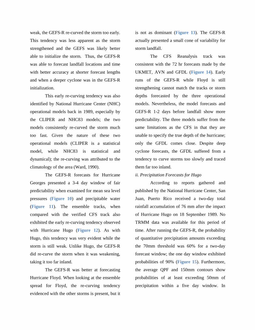
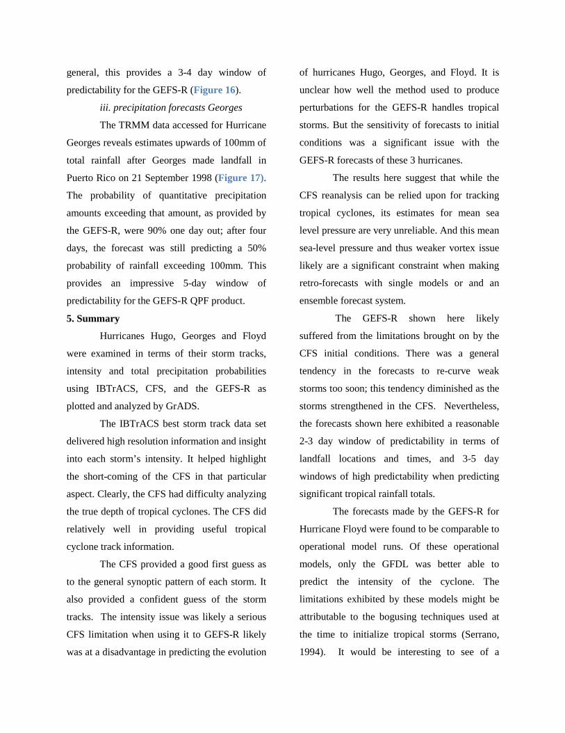
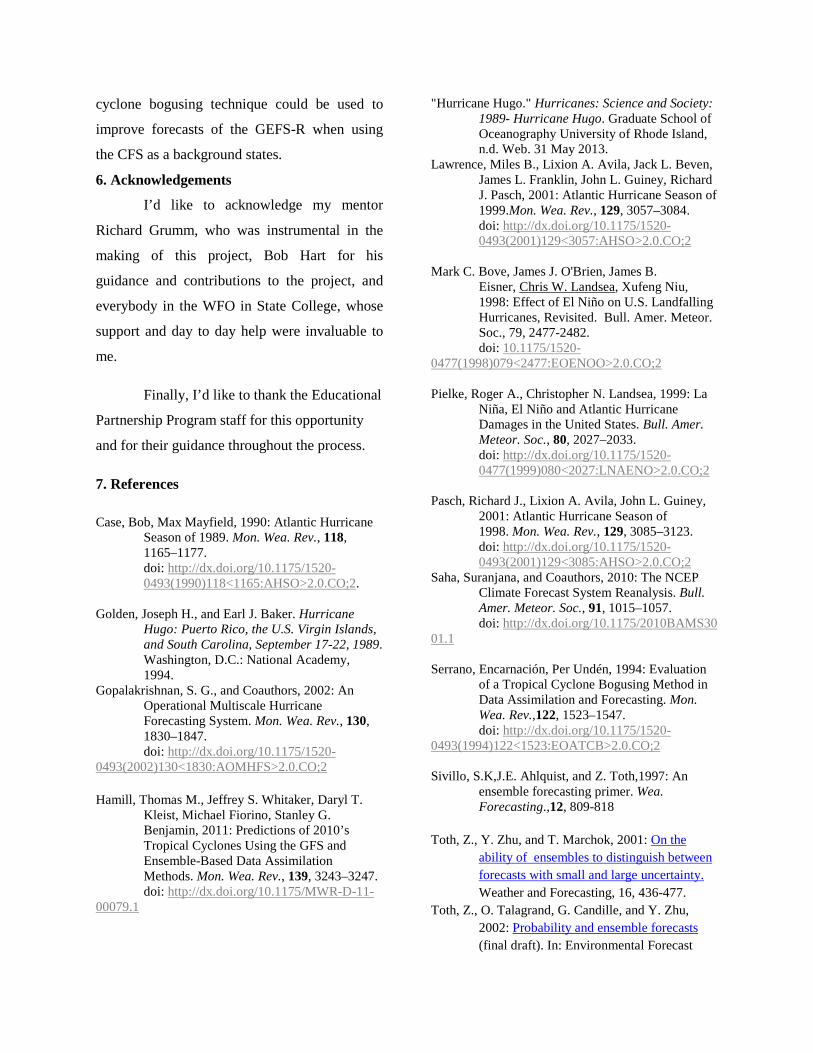
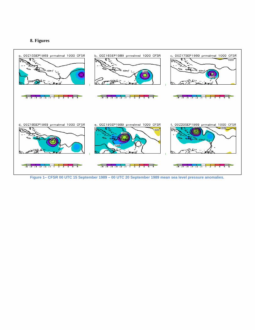
The decreased speed of Hugo only

helped prolong its impact on the Caribbean.

Moving at a 9 MPH, the eye of Hugo passed St.

Croix on the 18th, with winds of 61.73 m/s (120

kts). Just twelve hours later, satellite imagery

placed the eye of Hugo grazing the eastern coast

of Puerto Rico with winds of 53.5 m/s (104 kts).

After crossing Puerto Rico, the storm gained

forward speed but weakened substantially.

(Figure 1)

After affecting the Caribbean, Hugo

entered the open Atlantic, gaining strength and

by 20 September, the hurricane exhibited a more

organized eye and increased forward speeds. As

it reached the Gulf Stream, its forward speed and

wind speed dramatically increased. Hugo

became a Category 4 hurricane for the second

time in its life cycle. On September 22, Hugo

made landfall on the coast of South Carolina

near Charleston with a forward speed of 30

MPH and estimated maximum sustained winds

of 61.21 m/s (119 kts). Hugo then continued

inland as a tropical storm, before dissipating

over the far North Atlantic Ocean on 23

September. (Figure 2)

Rainfall amounts related to Hurricane

Hugo were reported in the range of 100-250mm

(4 to 10 inches) of rain in the Caribbean and the

Carolinas. Official reports from the National

Weather Service Weather Forecasting Office at

San Juan, PR established a rainfall total of 76

mm. In terms of storm surge, the Carolinas

experienced up to 6.1 m (20ft) surges in various

coastal areas. Florence and Sunter, North

Carolina reported tornadoes associated with the

storm as well. Damages caused by Hurricane

Hugo amounted to $9 billion dollars ($17.5

billion as of 2010, due to inflation).

B. Georges

Georges was first identified on 13

September, as a tropical wave exiting the coast

of Africa (Pasch, 2001). By 15 September, the

wave was classified as a tropical depression, and

it became a tropical storm by 16 September.

Georges reached hurricane strength around 1800

UTC on 17 September. It is estimated that

Georges reached a peak intensity of 69.45 m/s

(135 kts) winds at 0600 UTC on 20 September.

After that peak intensity on 20 September,

Georges began to weaken substantially, due to

upper-level vertical shear induced by an upper-

level anticyclone over the eastern Caribbean.

After this weakening, Georges made

landfall in Antigua and St Kitts and Nevis, with

maximum sustained surface winds of 51 m/s

(100 kts). It then made landfall in Puerto Rico

on 21 September, with sustained surface winds

of 51 m/s (100 kts). The interaction with the

orographic elements in the island weakened the

system slightly. After moving into the Mona

Passage on 22 September, Georges re-intensified

and made landfall about 75 miles east of Santo

Domingo with sustained surface winds of 54 m/s

(105 kts). (Figure 3)

Its subsequent passage through

Hispaniola during 22 -23 September continued to

weaken Georges, but it retained hurricane

strength while moving slowly west-

northwestward across the Windward Passage

and the northern coast of Cuba on 24 September.

Once back in open water, Georges began to re-

intensify. On 25 September, Georges made

landfall in Key West, Florida with a minimum

central pressure of 981 hPa and maximum winds

of 46 m/s (90 kts). During the next couple of

days, the system moved slowly towards

Mississippi, making landfall on the morning of

28 with a minimum central pressure of 964 hPa.

Georges was downgraded to tropical storm the

same day. Georges became semi stationary for

the next 12 hours, and then started moving in a

general northeastern direction on the 29

September. It was then downgraded to tropical

depression while located near Mobile, Alabama.

By early 1 October, the system had completely

dissipated near the coast of northeast Florida and

southeast Georgia.

Storm surges were reported in various

locations including Puerto Rico, the Florida

Keys, Louisiana, Mississippi, and Alabama,

with averages in the range of 1.22-3 m (4-10

feet). Fort Morgan, Alabama reported maximum

surge of 3.63 m (11.9 ft). In terms of

precipitation, the US Virgin Islands saw rainfall

totals between 50-200mm (2-8 inches), while in

Puerto Rico, the rainfall range fell between 250-

350mm (10 to 14 inches). Meanwhile, in the

Keys the maximum reported total was

212.85mm (8.34 inches). Georges also produced

twenty-eight tornadoes in the southeastern

region of United States.

Hurricane Georges exacted a high death

toll, with 602 reported deaths, most of them in

Hispaniola. Table 2 summarizes the storm-

related casualties. Total damages in the

Caribbean and the US reached the $6 billion

mark, with $3 billion of those happening in the

continental US and its territories.

C. Floyd

Floyd was first identified as a tropical

wave emerging from West Africa on 2

September. The system was disorganized and

showed little promise of convective

development. However, by 7 September the

wave had developed enough of a curved band of

deep convection and a consolidated cloud

pattern to be classified as a tropical depression.

It was later classified as Tropical Storm Floyd

on 8 September, about 750 miles east of the

Leeward Islands (Lawrence, 2001).

Floyd became a hurricane by 1200 UTC

10 September. It strengthened to category 3

during the next couple of days; however, it

interacted with the southwest portion of the mid-

Atlantic upper-troposphere trough, which

disrupted its upper level flow and caused it to

weaken on the 12th. After this weakening

episode, Floyd experienced a sustained

strengthening period, caused in part by its

westward motion and the presence of enhanced

upper ocean heat content in the area. By 1800

UTC 13 September, Floyd was a Category 4

tropical cyclone, with maximum sustained winds

of 70 m/s (135 kts).

Late on the 13th, Floyd blew over the

Bahamas, making landfall on Eleuthera by 14

September, later going on to strike Abaco in the

afternoon. It continued to move parallel to

Florida, headed straight to the Carolinas. Floyd

made landfall near Cape Fear, North Carolina by

600 UTC 16 September as a category 2

hurricane with estimated maximum winds near

46 m/s (90 kts). After making landfall, it

weakened substantially to become a tropical

storm, and then continued moving swiftly along

the coast of Delaware and New Jersey. It

reached Long Island by 0000 UTC 17

September. At this moment, Floyd became

involved with a frontal low over the Eastern

seaboard, and thus became an extratropical

system by 1200 UTC 17 September. By the 19

September, it was no longer a distinguishable

entity. (Figure 4)

Rainfall totals as high as 350 mm to

500mm (12 -14 inches) were reported in North

Carolina, Virginia, Maryland, Delaware and

New Jersey. In Philadelphia, a record was set for

most rain in a calendar day: 168.4 mm (6.61

inches). Storm surge of 2.5-3 m (9 to 10 ft)

experienced in the North Carolina coast. At least

15 tornadoes were reported in eastern North

Carolina and the Wilmington area. One of the

confirmed tornadoes destroyed two houses and

damaged four others.

Damages associated with Floyd ranged

between 3 and 6 billion dollars. Floyd caused 57

fatalities, 56 of which were in the United States

including 6 fatalities in Pennsylvania. Floyd was

the deadliest hurricane in the US since Agnes in

1972.

3. Methods

The tropical cyclones studied in this

project were selected based upon the following

criteria: they had to have occurred prior to the

implementation of the GEFS; they must have

reached Category 3 intensity as ranked by the

Saffir-Simpson scale; and they must have had a

significant impact on the Caribbean and

continental United States. Thus, Hurricane Hugo

(1989), Georges (1998), Floyd (1999), and Fran

(1996) were chosen.

Various datasets were obtained,

including the CFS reanalysis for the dates

chosen, the GEFS-R forecasts for the same

periods of time, total rainfall amounts as

measured by the Tropical Rainfall Measuring

Mission (TRMM) and the best cyclone tracks

from the International Best Track Archive for

Climate Stewardship (IBTrACS). Not all

datasets spanned the years of the studied storms.

For example, Hugo occurred before the

evolution of TRMM data. All of the data were

plotted and analyzed using the Grid Analysis

and Display System (GrADS) desktop tool. Post

analysis data and some plots were made using

Excel.

The CFS reanalysis data was used to

obtain a close approximation of the actual

atmospheric conditions at the times of the

storms, and provided a control to visualize each

storm. Some of the parameters plotted and

analyzed from the dataset were mean sea level

pressure (MSLP), 850mb heights, and the

precipitable water (PW). These data were plotted

along with departures from normal of these data

in standard deviations from normal as described

by Hart and Grumm (2001).

The GEFS-R forecast data was plotted

and analyzed for the same parameters.

Additionally, track and intensity data were

obtained from the two datasets using GrADS to

obtained the lowest pressure and estimate the

winds near the point with the lower MSLP. The

grid point data obtained using this method were

put into Excel to compare to other datasets and

to produce the track forecasts.

The GEFS-R forecast of quantitative

precipitation (QPF) were also analyzed and

plotted in GrADS. The probabilities of the QPF

exceeding various thresholds were computed

along with the GEFS-R mean QPF. These data

were compared to available verification data to

qualitatively assess the ability of the GEFS-R to

predicted areas of heavy rainfall associated with

each system. The best storm track data from

IBTrACS provided verified and reliable storm

track and intensity data that could be used on a

control basis for comparison against the GEFS-

R and the CFS. The data included coordinates,

mean sea level pressures, maximum sustained

winds, and storm intensity as described by the

Saffir Simpson scale. This was compared with

the track and intensity data from the CFS and the

GEFS-R.

The same process was used when

studying data for Hurricane Floyd from three

operational models: the UKMET, the AVN (now

GFS), and the GFDL. Track and intensity data

was obtained from the model, and compared to

verify for accuracy. In order to better understand

the statistical nature of the data studied,

Microsoft Excel was used to run statistical

analysis of the average errors.

4. Results and Discussion

i. Track and Intensity Forecasts

When comparing the CFS tracks for

Hugo to the IBTrACS best track data (Figure 5),

it’s evident that the CFS has considerable skill in

matching the path of the storm. A similar

behavior could be observed when the CFS tracks

for Georges (Figure 6) and Floyd (Figure 7)

were compared to the IBTrACS data.

For Hurricane Hugo, the average error

for the location of the storm at any given time

was about 20 km. In Georges’ case, the average

error for latitude and longitudes was about 30

km in any direction. Finally, for Hurricane Floyd

the average error was also approximately 30 km.

All values fall within the 95% confidence

interval. This validates the CFS’ ability to

correctly approximate the position of the storm

at any given time.

Point data for mean sea level pressure

from the CFS reanalysis and the IBTrACS were

compared for all storms. The differences

between the reanalysis values and the measured

values were considerable. These data showed

that the CFS had a limited ability to capture the

intensity of tropical storms. The pressure

differences for Hurricane Hugo were the most

noticeable. At its most intense moment, the CFS

was estimating a storm with pressures 66 hPa

greater than the measured values (Table 1). In

general, the CFS consistently underestimated

Hugo’s depth. The same behavior was observed

for Georges; the storm was estimated to be

between 30 to 70 hPa weaker than it actually

was (Table 2). Floyd was no exception; the

storm was also estimated to be up to 50 hPa

weaker than measured (Table 3). The CFS was

unable to obtain the intensity of tropical

cyclones relative to the IBTrACS data.

Maximum sustained winds point data

were also compared for Hurricane Hugo (Table

4). The data reflected significant departures in

the CFS estimates from the IBTrACS expected

values (at its strongest point, the CFS estimated

winds 40 knots below the observed values; at its

weakest, it was overestimating by 30 knots).

After establishing the quality and

limitations of the CFS reanalysis data, the

GEFS-R forecasts were examined. When

looking at Hurricane Hugo’s forecasts for

landfall in Puerto Rico (by 0000 UTC 18

September 1989), a 2-3 day window of

predictability was evident (Figure 8).

As expected, these forecasts show that

longer range predictions had larger errors. For

example, the GEFS-R initialized at 19

September 0000 UTC (Figure 8.f) had a weaker

cyclone northeast of Puerto Rico while shorter

range forecasts (Figure 8.a) showed a

significantly deeper storm. The ensemble mean

and spread diagrams (not shown) indicated

higher uncertainty in the longer range forecasts.

This uncertainty information could be obtained

by visually inspecting the track forecasts

(Figure 9) which show larger spread in the

tracks from earlier over the Eastern Caribbean

and the Leeward islands versus tracks from later

forecasts further west. The storm tracks garnered

for the 6-day period showed that during the early

stages of formation, when the storm was still

weak, the GEFS-R re-curved the storm too early.

This tendency was less apparent as the storm

strengthened and the GEFS was likely better

able to initialize the storm. Thus, the GEFS-R

was able to forecast landfall locations and time

with better accuracy at shorter forecast lengths

and when a deeper cyclone was in the GEFS-R

initialization.

This early re-curving tendency was also

identified by National Hurricane Center (NHC)

operational models back in 1989, especially by

the CLIPER and NHC83 models; the two

models consistently re-curved the storm much

too fast. Given the nature of these two

operational models (CLIPER is a statistical

model, while NHC83 is statistical and

dynamical); the re-curving was attributed to the

climatology of the area (Ward, 1990).

The GEFS-R forecasts for Hurricane

Georges presented a 3-4 day window of fair

predictability when examined for mean sea level

pressures (Figure 10) and precipitable water

(Figure 11). The ensemble tracks, when

compared with the verified CFS track also

exhibited the early re-curving tendency observed

with Hurricane Hugo (Figure 12). As with

Hugo, this tendency was very evident while the

storm is still weak. Unlike Hugo, the GEFS-R

did re-curve the storm when it was weakening,

taking it too far inland.

The GEFS-R was better at forecasting

Hurricane Floyd. When looking at the ensemble

spread for Floyd, the re-curving tendency

evidenced with the other storms is present, but it

is not as dominant (Figure 13). The GEFS-R

actually presented a small cone of variability for

storm landfall.

The CFS Reanalysis track was

consistent with the 72 hr forecasts made by the

UKMET, AVN and GFDL (Figure 14). Early

runs of the GEFS-R while Floyd is still

strengthening cannot match the tracks or storm

depths forecasted by the three operational

models. Nevertheless, the model forecasts and

GEFS-R 1-2 days before landfall show more

predictability. The three models suffer from the

same limitations as the CFS in that they are

unable to specify the true depth of the hurricane;

only the GFDL comes close. Despite deep

cyclone forecasts, the GFDL suffered from a

tendency to curve storms too slowly and traced

them far too inland.

ii. Precipitation Forecasts for Hugo

According to reports gathered and

published by the National Hurricane Center, San

Juan, Puerto Rico received a two-day total

rainfall accumulation of 76 mm after the impact

of Hurricane Hugo on 18 September 1989. No

TRMM data was available for this period of

time. After running the GEFS-R, the probability

of quantitative precipitation amounts exceeding

the 70mm threshold was 60% for a two-day

forecast window; the one day window exhibited

probabilities of 90% (Figure 15). Furthermore,

the average QPF and 150mm contours show

probabilities of at least exceeding 50mm of

precipitation within a five day window. In

general, this provides a 3-4 day window of

predictability for the GEFS-R (Figure 16).

iii. precipitation forecasts Georges

The TRMM data accessed for Hurricane

Georges reveals estimates upwards of 100mm of

total rainfall after Georges made landfall in

Puerto Rico on 21 September 1998 (Figure 17).

The probability of quantitative precipitation

amounts exceeding that amount, as provided by

the GEFS-R, were 90% one day out; after four

days, the forecast was still predicting a 50%

probability of rainfall exceeding 100mm. This

provides an impressive 5-day window of

predictability for the GEFS-R QPF product.

5. Summary

Hurricanes Hugo, Georges and Floyd

were examined in terms of their storm tracks,

intensity and total precipitation probabilities

using IBTrACS, CFS, and the GEFS-R as

plotted and analyzed by GrADS.

The IBTrACS best storm track data set

delivered high resolution information and insight

into each storm’s intensity. It helped highlight

the short-coming of the CFS in that particular

aspect. Clearly, the CFS had difficulty analyzing

the true depth of tropical cyclones. The CFS did

relatively well in providing useful tropical

cyclone track information.

The CFS provided a good first guess as

to the general synoptic pattern of each storm. It

also provided a confident guess of the storm

tracks. The intensity issue was likely a serious

CFS limitation when using it to GEFS-R likely

was at a disadvantage in predicting the evolution

of hurricanes Hugo, Georges, and Floyd. It is

unclear how well the method used to produce

perturbations for the GEFS-R handles tropical

storms. But the sensitivity of forecasts to initial

conditions was a significant issue with the

GEFS-R forecasts of these 3 hurricanes.

The results here suggest that while the

CFS reanalysis can be relied upon for tracking

tropical cyclones, its estimates for mean sea

level pressure are very unreliable. And this mean

sea-level pressure and thus weaker vortex issue

likely are a significant constraint when making

retro-forecasts with single models or and an

ensemble forecast system.

The GEFS-R shown here likely

suffered from the limitations brought on by the

CFS initial conditions. There was a general

tendency in the forecasts to re-curve weak

storms too soon; this tendency diminished as the

storms strengthened in the CFS. Nevertheless,

the forecasts shown here exhibited a reasonable

2-3 day window of predictability in terms of

landfall locations and times, and 3-5 day

windows of high predictability when predicting

significant tropical rainfall totals.

The forecasts made by the GEFS-R for

Hurricane Floyd were found to be comparable to

operational model runs. Of these operational

models, only the GFDL was better able to

predict the intensity of the cyclone. The

limitations exhibited by these models might be

attributable to the bogusing techniques used at

the time to initialize tropical storms (Serrano,

1994). It would be interesting to see of a

cyclone bogusing technique could be used to

improve forecasts of the GEFS-R when using

the CFS as a background states.

6. Acknowledgements

I’d like to acknowledge my mentor

Richard Grumm, who was instrumental in the

making of this project, Bob Hart for his

guidance and contributions to the project, and

everybody in the WFO in State College, whose

support and day to day help were invaluable to

me.

Finally, I’d like to thank the Educational

Partnership Program staff for this opportunity

and for their guidance throughout the process.

7. References Case, Bob, Max Mayfield, 1990: Atlantic Hurricane

Season of 1989. Mon. Wea. Rev., 118, 1165–1177. doi: http://dx.doi.org/10.1175/1520-0493(1990)118<1165:AHSO>2.0.CO;2.

Golden, Joseph H., and Earl J. Baker. Hurricane Hugo: Puerto Rico, the U.S. Virgin Islands, and South Carolina, September 17-22, 1989. Washington, D.C.: National Academy, 1994.

Gopalakrishnan, S. G., and Coauthors, 2002: An Operational Multiscale Hurricane Forecasting System. Mon. Wea. Rev., 130, 1830–1847. doi: http://dx.doi.org/10.1175/1520-

0493(2002)130<1830:AOMHFS>2.0.CO;2 Hamill, Thomas M., Jeffrey S. Whitaker, Daryl T.

Kleist, Michael Fiorino, Stanley G. Benjamin, 2011: Predictions of 2010’s Tropical Cyclones Using the GFS and Ensemble-Based Data Assimilation Methods. Mon. Wea. Rev., 139, 3243–3247. doi: http://dx.doi.org/10.1175/MWR-D-11-

00079.1

"Hurricane Hugo." Hurricanes: Science and Society: 1989- Hurricane Hugo. Graduate School of Oceanography University of Rhode Island, n.d. Web. 31 May 2013.

Lawrence, Miles B., Lixion A. Avila, Jack L. Beven, James L. Franklin, John L. Guiney, Richard J. Pasch, 2001: Atlantic Hurricane Season of 1999.Mon. Wea. Rev., 129, 3057–3084. doi: http://dx.doi.org/10.1175/1520-0493(2001)129<3057:AHSO>2.0.CO;2

Mark C. Bove, James J. O'Brien, James B.

Eisner, Chris W. Landsea, Xufeng Niu, 1998: Effect of El Niño on U.S. Landfalling Hurricanes, Revisited. Bull. Amer. Meteor. Soc., 79, 2477-2482. doi: 10.1175/1520-

0477(1998)079<2477:EOENOO>2.0.CO;2 Pielke, Roger A., Christopher N. Landsea, 1999: La

Niña, El Niño and Atlantic Hurricane Damages in the United States. Bull. Amer. Meteor. Soc., 80, 2027–2033. doi: http://dx.doi.org/10.1175/1520-0477(1999)080<2027:LNAENO>2.0.CO;2

Pasch, Richard J., Lixion A. Avila, John L. Guiney,

2001: Atlantic Hurricane Season of 1998. Mon. Wea. Rev., 129, 3085–3123. doi: http://dx.doi.org/10.1175/1520-0493(2001)129<3085:AHSO>2.0.CO;2

Saha, Suranjana, and Coauthors, 2010: The NCEP Climate Forecast System Reanalysis. Bull. Amer. Meteor. Soc., 91, 1015–1057. doi: http://dx.doi.org/10.1175/2010BAMS30

01.1 Serrano, Encarnación, Per Undén, 1994: Evaluation

of a Tropical Cyclone Bogusing Method in Data Assimilation and Forecasting. Mon. Wea. Rev.,122, 1523–1547. doi: http://dx.doi.org/10.1175/1520-

0493(1994)122<1523:EOATCB>2.0.CO;2 Sivillo, S.K,J.E. Ahlquist, and Z. Toth,1997: An

ensemble forecasting primer. Wea. Forecasting.,12, 809-818

Toth, Z., Y. Zhu, and T. Marchok, 2001: On the

ability of ensembles to distinguish between forecasts with small and large uncertainty. Weather and Forecasting, 16, 436-477.

Toth, Z., O. Talagrand, G. Candille, and Y. Zhu, 2002: Probability and ensemble forecasts (final draft). In: Environmental Forecast

Verification: A practitioner's guide in atmospheric science. Ed.: I. T. Jolliffe and D. B. Stephenson. Wiley, pp.137-164.

Ward, J.H,1990:A Review of Numerical Forecast

Guidance for Hurricane Hugo.Wea. and Fore., 5, 416-32.

Wei, M. and Z. Toth, R.Wobus, Y.Zhu, C.H.Bishop, X. Wang 2006: Ensemble Transform

Kalman Filter-based ensemble perturbations in an operational global prediction system at NCEP, Tellus 58A, 28-44 . (text and figures in PDF).

Wei, M. and Z. Toth, R.Wobus, Y.Zhu, 2008: Initial perturbations based on the ensemble transform (ET) technique in the NCEP global operational forecast system. Tellus, 60A, 62–79. pdf

8. Figures

Figure 1– CFSR 00 UTC 15 September 1989 – 00 UTC 20 September 1989 mean sea level pressure anomalies.

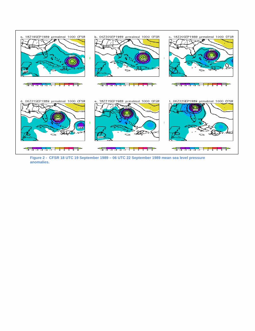
Figure 2 - CFSR 18 UTC 19 September 1989 – 06 UTC 22 September 1989 mean sea level pressure anomalies.

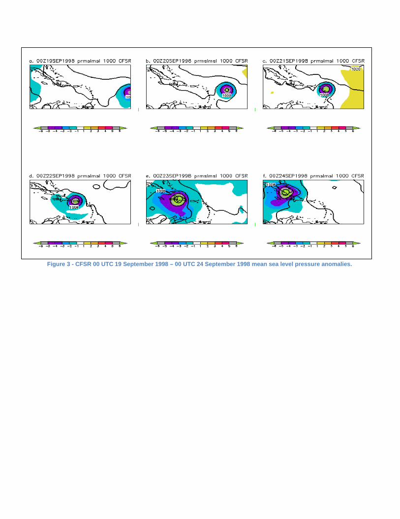
Figure 3 - CFSR 00 UTC 19 September 1998 – 00 UTC 24 September 1998 mean sea level pressure anomalies.

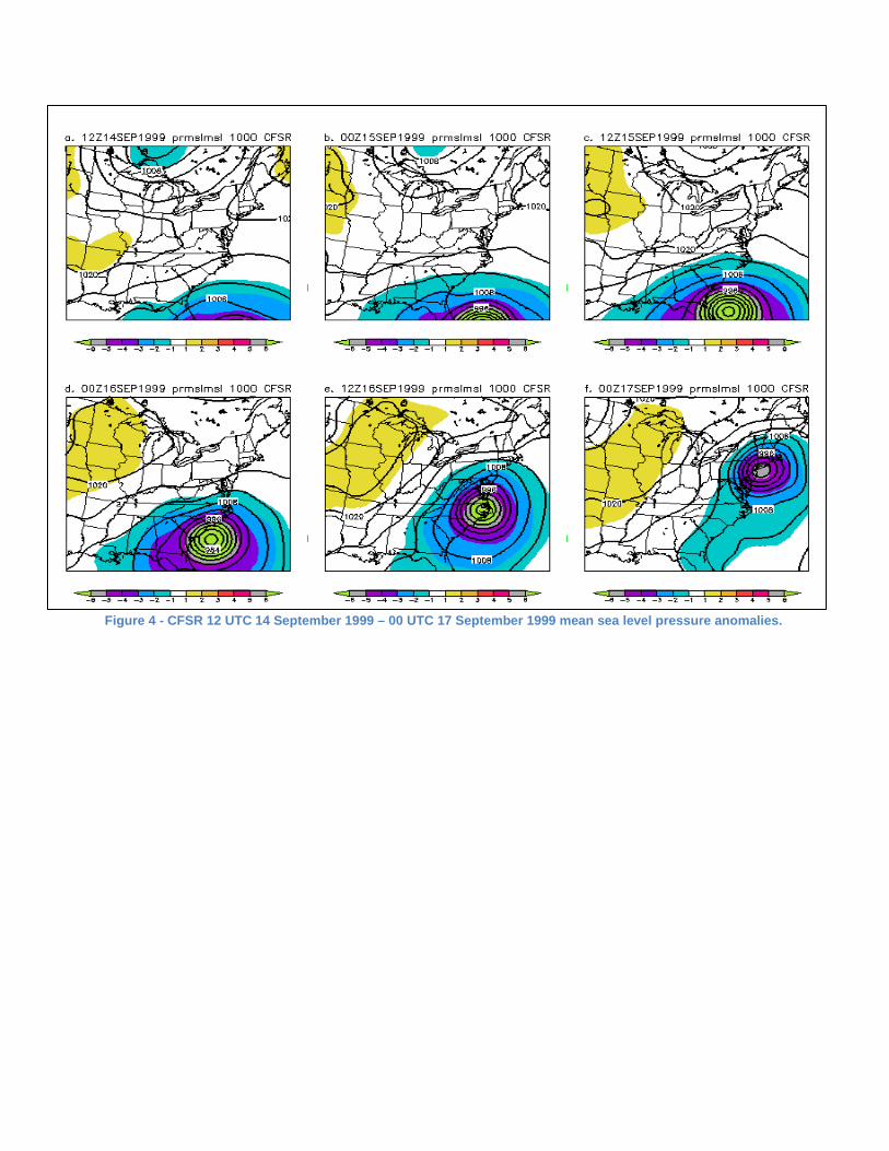
Figure 4 - CFSR 12 UTC 14 September 1999 – 00 UTC 17 September 1999 mean sea level pressure anomalies.

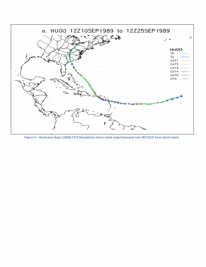
Figure 5 - Hurricane Hugo (1989) CFS Reanalysis storm track superimposed over IBTrACS best storm track.

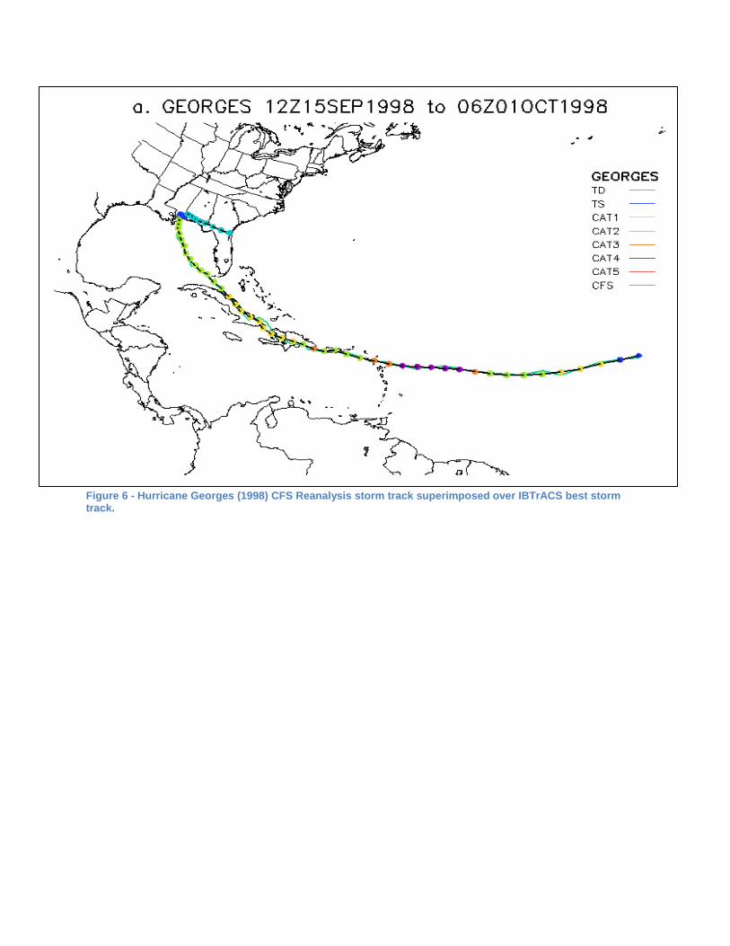
Figure 6 - Hurricane Georges (1998) CFS Reanalysis storm track superimposed over IBTrACS best storm track.

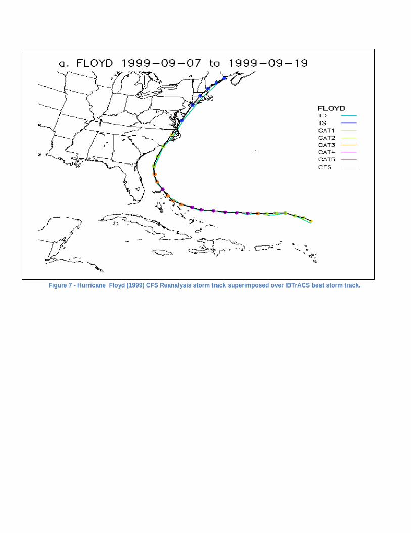
Figure 7 - Hurricane Floyd (1999) CFS Reanalysis storm track superimposed over IBTrACS best storm track.

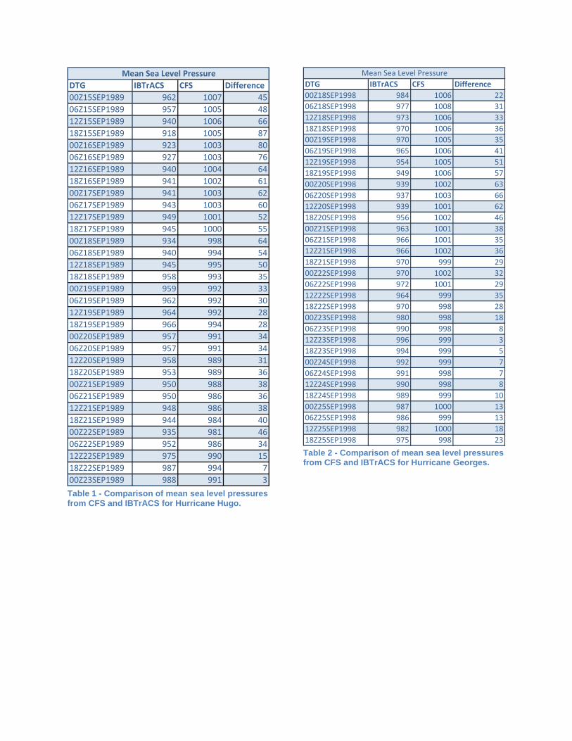
Table 1 - Comparison of mean sea level pressures from CFS and IBTrACS for Hurricane Hugo.

Table 2 - Comparison of mean sea level pressures from CFS and IBTrACS for Hurricane Georges.

DTG IBTrACS CFS Difference00Z15SEP1989 962 1007 4506Z15SEP1989 957 1005 4812Z15SEP1989 940 1006 6618Z15SEP1989 918 1005 8700Z16SEP1989 923 1003 8006Z16SEP1989 927 1003 7612Z16SEP1989 940 1004 6418Z16SEP1989 941 1002 6100Z17SEP1989 941 1003 6206Z17SEP1989 943 1003 6012Z17SEP1989 949 1001 5218Z17SEP1989 945 1000 5500Z18SEP1989 934 998 6406Z18SEP1989 940 994 5412Z18SEP1989 945 995 5018Z18SEP1989 958 993 3500Z19SEP1989 959 992 3306Z19SEP1989 962 992 3012Z19SEP1989 964 992 2818Z19SEP1989 966 994 2800Z20SEP1989 957 991 3406Z20SEP1989 957 991 3412Z20SEP1989 958 989 3118Z20SEP1989 953 989 3600Z21SEP1989 950 988 3806Z21SEP1989 950 986 3612Z21SEP1989 948 986 3818Z21SEP1989 944 984 4000Z22SEP1989 935 981 4606Z22SEP1989 952 986 3412Z22SEP1989 975 990 1518Z22SEP1989 987 994 700Z23SEP1989 988 991 3

Mean Sea Level PressureDTG IBTrACS CFS Difference00Z18SEP1998 984 1006 2206Z18SEP1998 977 1008 3112Z18SEP1998 973 1006 3318Z18SEP1998 970 1006 3600Z19SEP1998 970 1005 3506Z19SEP1998 965 1006 4112Z19SEP1998 954 1005 5118Z19SEP1998 949 1006 5700Z20SEP1998 939 1002 6306Z20SEP1998 937 1003 6612Z20SEP1998 939 1001 6218Z20SEP1998 956 1002 4600Z21SEP1998 963 1001 3806Z21SEP1998 966 1001 3512Z21SEP1998 966 1002 3618Z21SEP1998 970 999 2900Z22SEP1998 970 1002 3206Z22SEP1998 972 1001 2912Z22SEP1998 964 999 3518Z22SEP1998 970 998 2800Z23SEP1998 980 998 1806Z23SEP1998 990 998 812Z23SEP1998 996 999 318Z23SEP1998 994 999 500Z24SEP1998 992 999 706Z24SEP1998 991 998 712Z24SEP1998 990 998 818Z24SEP1998 989 999 1000Z25SEP1998 987 1000 1306Z25SEP1998 986 999 1312Z25SEP1998 982 1000 1818Z25SEP1998 975 998 23

Mean Sea Level Pressure

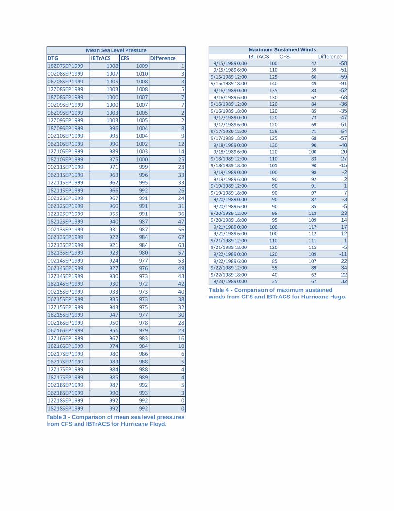
Table 3 - Comparison of mean sea level pressures from CFS and IBTrACS for Hurricane Floyd.

Table 4 - Comparison of maximum sustained winds from CFS and IBTrACS for Hurricane Hugo.

DTG IBTrACS CFS Difference18Z07SEP1999 1008 1009 100Z08SEP1999 1007 1010 306Z08SEP1999 1005 1008 312Z08SEP1999 1003 1008 518Z08SEP1999 1000 1007 700Z09SEP1999 1000 1007 706Z09SEP1999 1003 1005 212Z09SEP1999 1003 1005 218Z09SEP1999 996 1004 800Z10SEP1999 995 1004 906Z10SEP1999 990 1002 1212Z10SEP1999 989 1003 1418Z10SEP1999 975 1000 2500Z11SEP1999 971 999 2806Z11SEP1999 963 996 3312Z11SEP1999 962 995 3318Z11SEP1999 966 992 2600Z12SEP1999 967 991 2406Z12SEP1999 960 991 3112Z12SEP1999 955 991 3618Z12SEP1999 940 987 4700Z13SEP1999 931 987 5606Z13SEP1999 922 984 6212Z13SEP1999 921 984 6318Z13SEP1999 923 980 5700Z14SEP1999 924 977 5306Z14SEP1999 927 976 4912Z14SEP1999 930 973 4318Z14SEP1999 930 972 4200Z15SEP1999 933 973 4006Z15SEP1999 935 973 3812Z15SEP1999 943 975 3218Z15SEP1999 947 977 3000Z16SEP1999 950 978 2806Z16SEP1999 956 979 2312Z16SEP1999 967 983 1618Z16SEP1999 974 984 1000Z17SEP1999 980 986 606Z17SEP1999 983 988 512Z17SEP1999 984 988 418Z17SEP1999 985 989 400Z18SEP1999 987 992 506Z18SEP1999 990 993 312Z18SEP1999 992 992 018Z18SEP1999 992 992 0

Mean Sea Level Pressure Maximum Sustained WindsIBTrACS CFS Difference

9/15/1989 0:00 100 42 -589/15/1989 6:00 110 59 -51

9/15/1989 12:00 125 66 -599/15/1989 18:00 140 49 -91

9/16/1989 0:00 135 83 -529/16/1989 6:00 130 62 -68

9/16/1989 12:00 120 84 -369/16/1989 18:00 120 85 -35

9/17/1989 0:00 120 73 -479/17/1989 6:00 120 69 -51

9/17/1989 12:00 125 71 -549/17/1989 18:00 125 68 -57

9/18/1989 0:00 130 90 -409/18/1989 6:00 120 100 -20

9/18/1989 12:00 110 83 -279/18/1989 18:00 105 90 -15

9/19/1989 0:00 100 98 -29/19/1989 6:00 90 92 2

9/19/1989 12:00 90 91 19/19/1989 18:00 90 97 7

9/20/1989 0:00 90 87 -39/20/1989 6:00 90 85 -5

9/20/1989 12:00 95 118 239/20/1989 18:00 95 109 14

9/21/1989 0:00 100 117 179/21/1989 6:00 100 112 12

9/21/1989 12:00 110 111 19/21/1989 18:00 120 115 -5

9/22/1989 0:00 120 109 -119/22/1989 6:00 85 107 22

9/22/1989 12:00 55 89 349/22/1989 18:00 40 62 22

9/23/1989 0:00 35 67 32

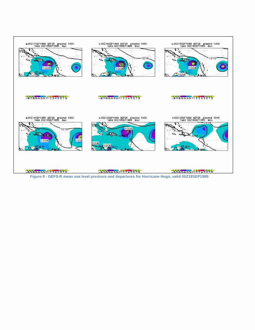
Figure 8 - GEFS-R mean sea level pressure and departures for Hurricane Hugo, valid 00Z18SEP1989.

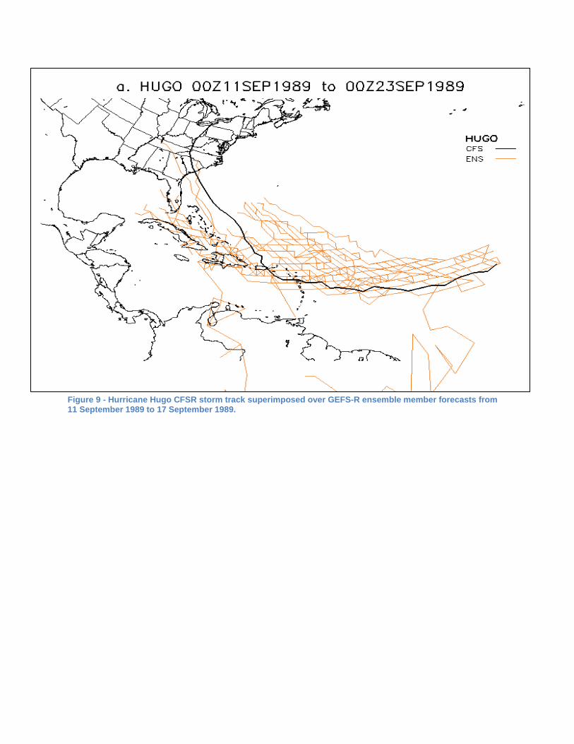
Figure 9 - Hurricane Hugo CFSR storm track superimposed over GEFS-R ensemble member forecasts from 11 September 1989 to 17 September 1989.

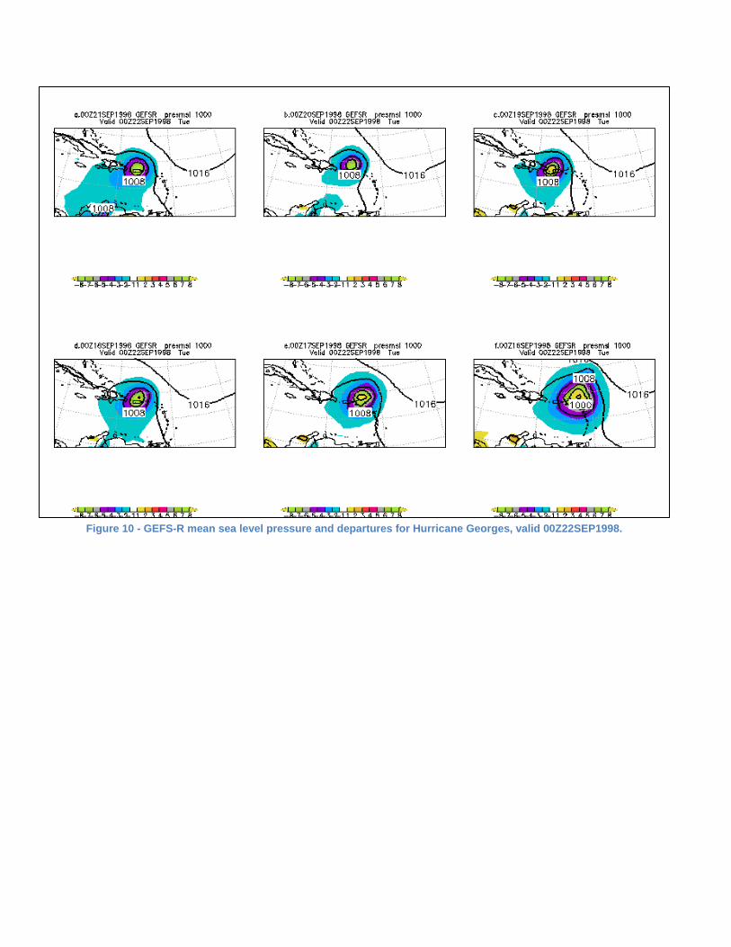
Figure 10 - GEFS-R mean sea level pressure and departures for Hurricane Georges, valid 00Z22SEP1998.

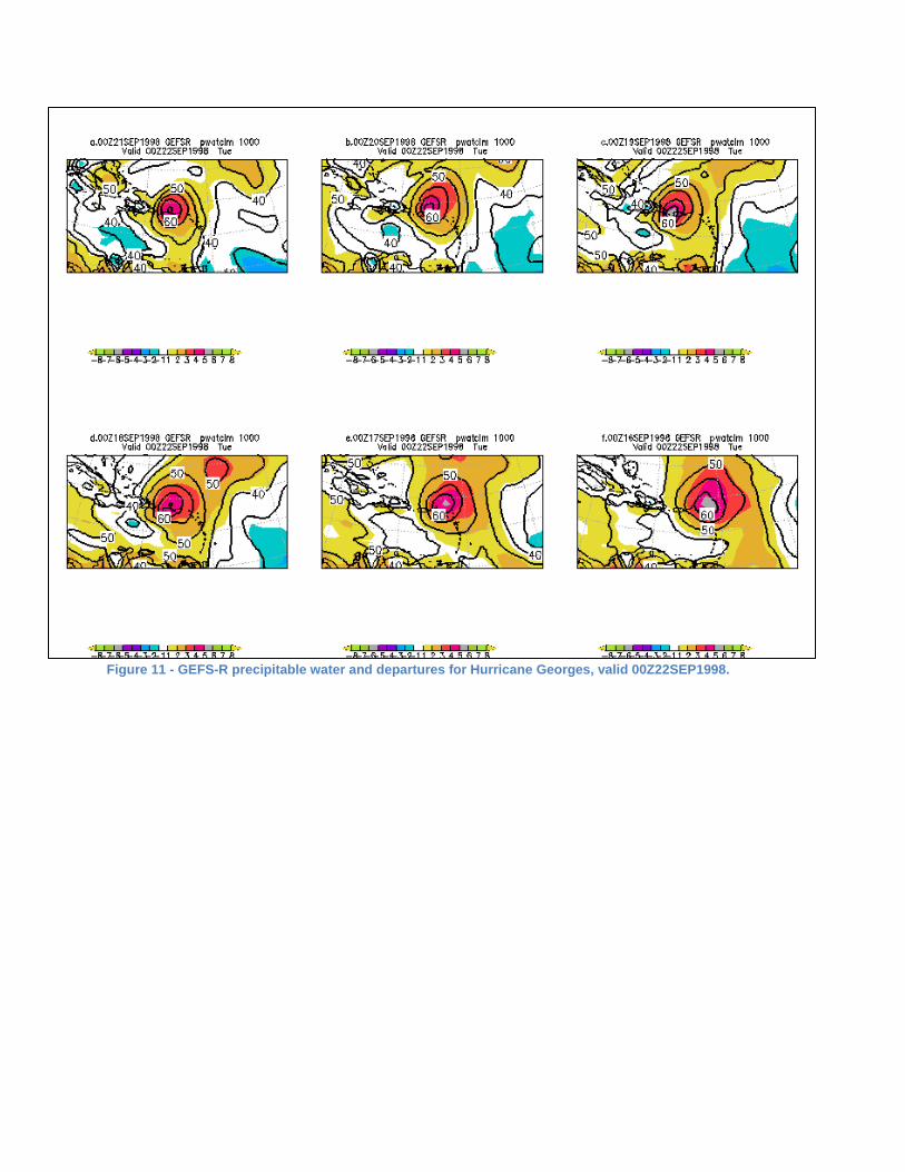
Figure 11 - GEFS-R precipitable water and departures for Hurricane Georges, valid 00Z22SEP1998.

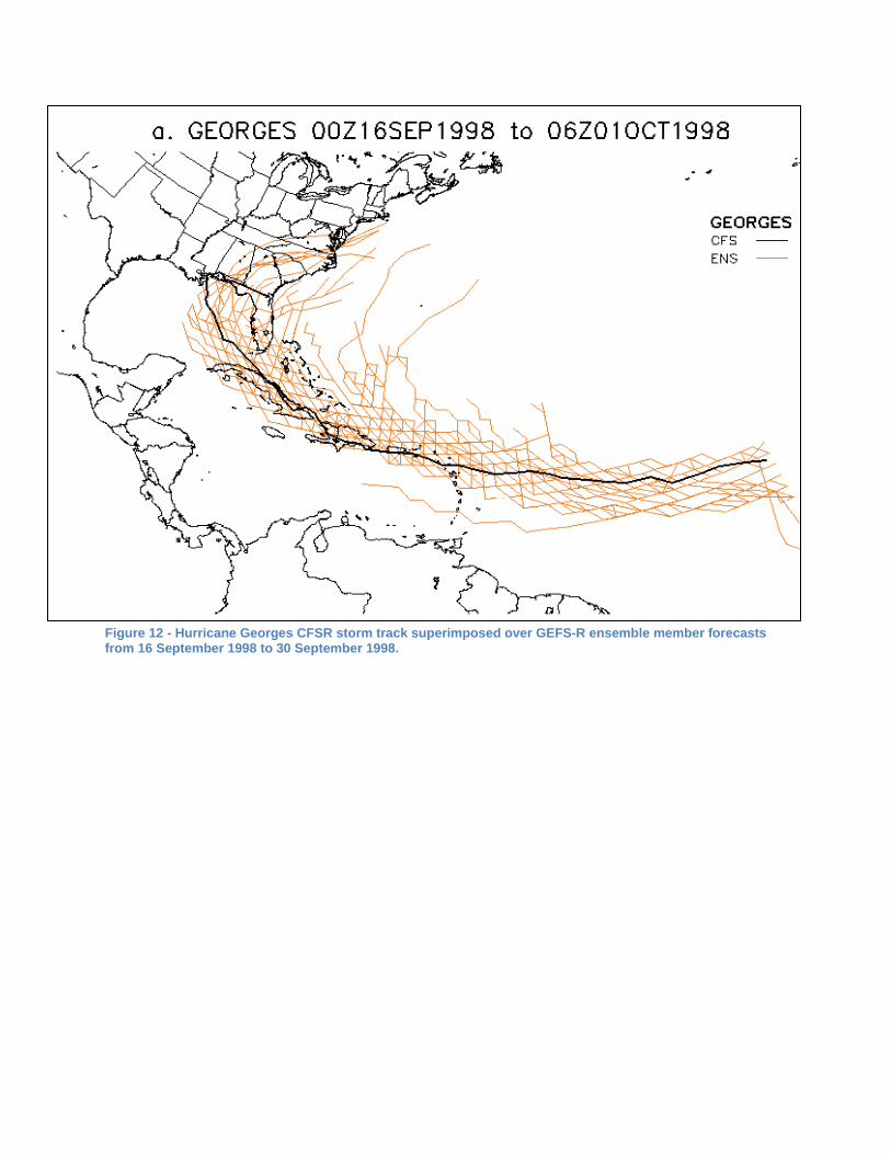
Figure 12 - Hurricane Georges CFSR storm track superimposed over GEFS-R ensemble member forecasts from 16 September 1998 to 30 September 1998.

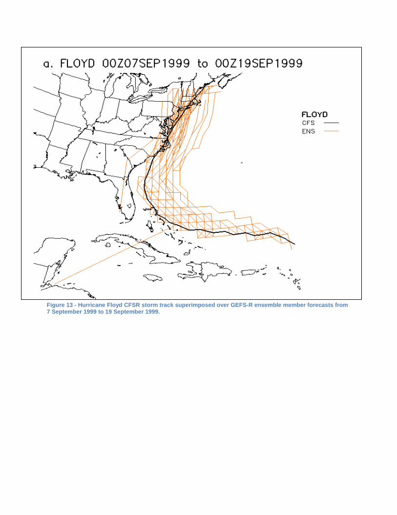
Figure 13 - Hurricane Floyd CFSR storm track superimposed over GEFS-R ensemble member forecasts from 7 September 1999 to 19 September 1999.

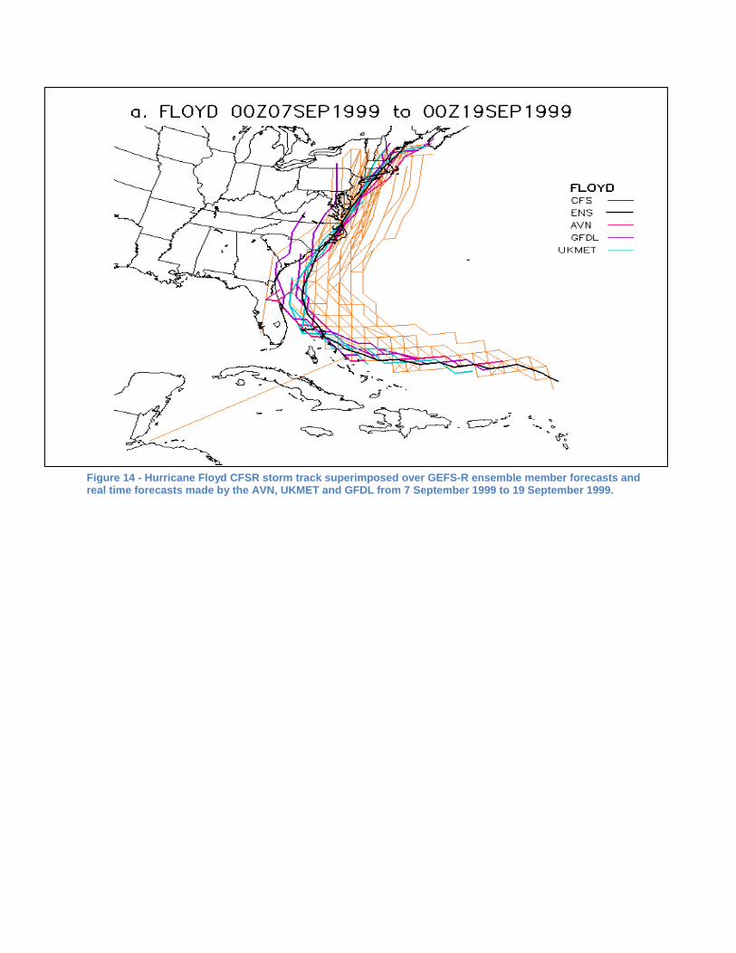
Figure 14 - Hurricane Floyd CFSR storm track superimposed over GEFS-R ensemble member forecasts and real time forecasts made by the AVN, UKMET and GFDL from 7 September 1999 to 19 September 1999.

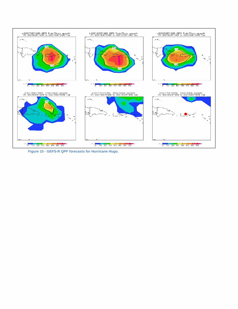
Figure 15 - GEFS-R QPF forecasts for Hurricane Hugo.

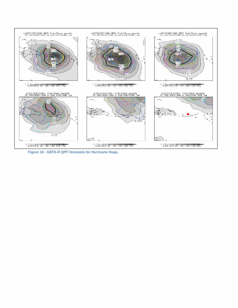
Figure 16 - GEFS-R QPF forecasts for Hurricane Hugo.

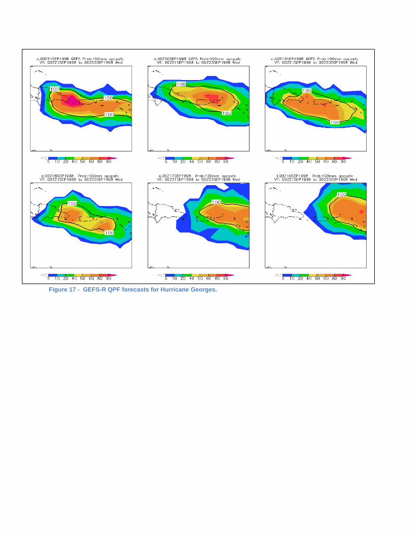
Figure 17 - GEFS-R QPF forecasts for Hurricane Georges.