1

Ensemble forecasting and data assimilation: two problems with the same solution?

Eugenia Kalnay

Department of Meteorology and Chaos Group University of Maryland, College Park, MD, 20742

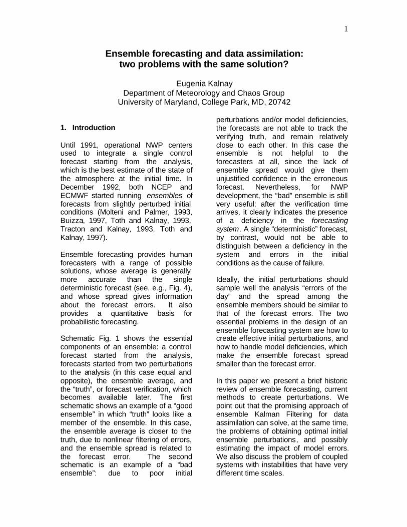
1. Introduction Until 1991, operational NWP centers used to integrate a single control forecast starting from the analysis, which is the best estimate of the state of the atmosphere at the initial time. In December 1992, both NCEP and ECMWF started running ensembles of forecasts from slightly perturbed initial conditions (Molteni and Palmer, 1993, Buizza, 1997, Toth and Kalnay, 1993, Tracton and Kalnay, 1993, Toth and Kalnay, 1997). Ensemble forecasting provides human forecasters with a range of possible solutions, whose average is generally more accurate than the single deterministic forecast (see, e.g., Fig. 4), and whose spread gives information about the forecast errors. It also provides a quantitative basis for probabilistic forecasting. Schematic Fig. 1 shows the essential components of an ensemble: a control forecast started from the analysis, forecasts started from two perturbations to the analysis (in this case equal and opposite), the ensemble average, and the “truth”, or forecast verification, which becomes available later. The first schematic shows an example of a “good ensemble” in which “truth” looks like a member of the ensemble. In this case, the ensemble average is closer to the truth, due to nonlinear filtering of errors, and the ensemble spread is related to the forecast error. The second schematic is an example of a “bad ensemble”: due to poor initial

perturbations and/or model deficiencies, the forecasts are not able to track the verifying truth, and remain relatively close to each other. In this case the ensemble is not helpful to the forecasters at all, since the lack of ensemble spread would give them unjustified confidence in the erroneous forecast. Nevertheless, for NWP development, the “bad” ensemble is still very useful: after the verification time arrives, it clearly indicates the presence of a deficiency in the forecasting system . A single “deterministic” forecast, by contrast, would not be able to distinguish between a deficiency in the system and errors in the initial conditions as the cause of failure. Ideally, the initial perturbations should sample well the analysis “errors of the day” and the spread among the ensemble members should be similar to that of the forecast errors. The two essential problems in the design of an ensemble forecasting system are how to create effective initial perturbations, and how to handle model deficiencies, which make the ensemble forecast spread smaller than the forecast error. In this paper we present a brief historic review of ensemble forecasting, current methods to create perturbations. We point out that the promising approach of ensemble Kalman Filtering for data assimilation can solve, at the same time, the problems of obtaining optimal initial ensemble perturbations, and possibly estimating the impact of model errors. We also discuss the problem of coupled systems with instabilities that have very different time scales.

2

Bad ensemble POSITIVE PERTURBATION

NEGATIVE PERTURBATION

CONTROL

AVERAGE

TRUTH

CONTROL

TRUTH

ENSEMBLE AVERAGE

POSITIVE PERTURBATION

NEGATIVE PERTURBATION

Good ensemble

Figure 1: Schematic of the essential components of an ensemble of forecasts: The analysis (a cross) which constitutes the initial conditions for the control forecast (in green); the initial perturbations (a thick dot) around the analysis, which in this case are chosen to be equal and opposite; the perturbed forecasts (in black); the ensemble average (in blue); and the verifying analysis or truth (in red). The first schematic is that of a “good ensemble” in which the truth is a plausible member of the ensemble. The second is an example of a bad ensemble, quite different from the truth, pointing to the presence of a problem in the forecasting system such as deficiencies in the analysis, in the ensemble perturbations and/or in the model.

3

2. Ensemble forecasting methods It should be noted that human forecasters have always performed subjective ensemble forecasting by checking forecasts from previous days, and comparing forecasts from different centers, approaches similar to lagged forecasting and multiple systems forecasting. The consistency among these forecasts at a given verification time provided a level of confidence in the forecasts, confidence that changed from day to day and from region to region. 2.1 Early methods Epstein (1969), introduced the idea of Stochastic-Dynamic forecasting (SDF), and pointed out that it could be also used in the analysis cycle to provide the forecast error covariance. Epstein designed SDF as a shortcut to estimate the true probability distribution of the forecast uncertainty, given by the Liouville equation (Ehrendorfer, 2002), which Epstein approximated running a huge (500) number of perturbed (Monte Carlo) integrations for the 3-variable Lorenz (1963) model. However, since SDF involves the integration of forecast equations for each element of the covariance matrix, this method is still not computationally feasible for models with large number of degrees of freedom. Leith (1974) suggested using directly a Monte Carlo Forecasting approach (MCF), where random perturbations sampling the estimated analysis error covariance are added to the initial conditions. He noted that in an infinitely large ensemble, the average forecast error variance at long time leads converges to the climatological error variance, whereas the error variance of individual forecasts converges to twice the climatological error variance. Leith showed that with just a relatively small

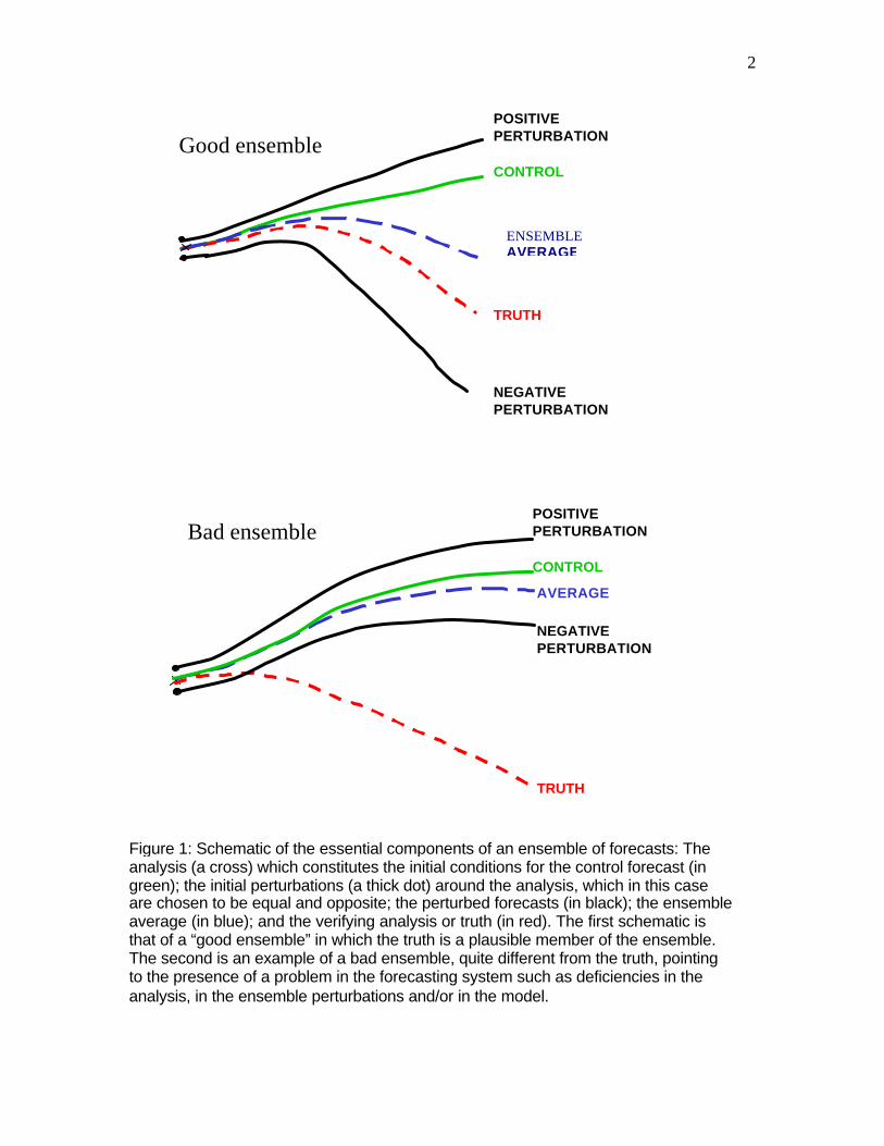
number of integrations (of the order of 8) it is possible to approximate this important advantage of an infinite ensemble. The estimate of the analysis error covariance was constant in time, so the MCF method did not include the effects of “errors of the day”. The MCF method is shown schematically in Fig. 2a. Errico and Baumhefner (1987) applied this method to realistic global models, using perturbations that represented a realistic (but constant) estimation of the errors in the initial conditions. Hollingsworth (1980) showed that random errors in the initial conditions took too long to spin-up into growing “errors of the day”, making MCF an inefficient approach for ensemble forecasting. Hoffman and Kalnay (1983) suggested as an alternative to MCF, the Lagged Averaged Forecasting (LAF) method, in which forecasts from earlier analyses were included in the ensemble (schematic Fig. 2b). Since the ensemble members are forecasts of different “ages” they should be averaged with weights estimated from their average forecast errors. Hoffman and Kalnay found that compared to MCF, LAF resulted in a better prediction of skill (a stronger relationship between ensemble spread and error), presumably because LAF includes the effect of variable “errors of the day”. The main disadvantage of LAF, that the “older” forecasts are less accurate, was corrected by the Scaled LAF (SLAF) approach of Ebisuzaki and Kalnay (1991), in which the LAF perturbations (difference between the forecast and the current analysis) are scaled by their “age”, so that all the SLAF perturbations have errors of similar magnitude. They also suggested that the scaled perturbations should be both added and subtracted from the analysis, thus increasing the ensemble size and the probability of “encompassing” the true

4

solution within the ensemble. SLAF can be easily implemented in both global and regional models, including the

impact of perturbed boundary conditions (Hou et al, 2001).

t tf -3dt 0 -dt -2dt

LAF X

t tf 0

MCF X

Fig. 2: Schematic of the Monte Carlo forecasting and Lagged Average Forecasting methods.

5

2.2 Operational Ensemble Forecasting methods In December 1992 two methods to create perturbations became operational at NCEP and at ECMWF. They are based on bred vectors and singular vectors respectively, and like LAF, they include “errors of the day”. These and other methods that have since become operational or are under consideration in operational centers are briefly discussed. More details are given in Kalnay (2003). a. Singular Vectors (SVs) Singular vectors are the linear perturbations of a control forecast that grow fastest within a certain time interval (Lorenz, 1965), known as “optimization period”, using a specific norm to measure their size. SVs are strongly sensitive to the length of the interval and to the choice of norm (Ahlquist, 2000). Ehrendorfer and Tribbia (1997) showed that if the initial norm used to derive the singular vectors is the analysis error covariance norm, then the initial singular vectors evolve into the eigenvectors of the forecast error covariance at the end of the optimization period. This indicates that if the analysis error covariance is known, then singular vectors based on this specific norm are the ideal perturbations. ECMWF implemented an ensemble system with initial perturbations based on singular vectors using a total energy norm (Molteni and Palmer, 1993, Molteni et al, 1996, Buizza et al, 1997, Palmer et al 1998). b. Bred Vectors (BVs) Breeding is a nonlinear generalization of the method to obtain leading Lyapunov vectors, which are the sustained fastest growing perturbations (Toth and Kalnay,

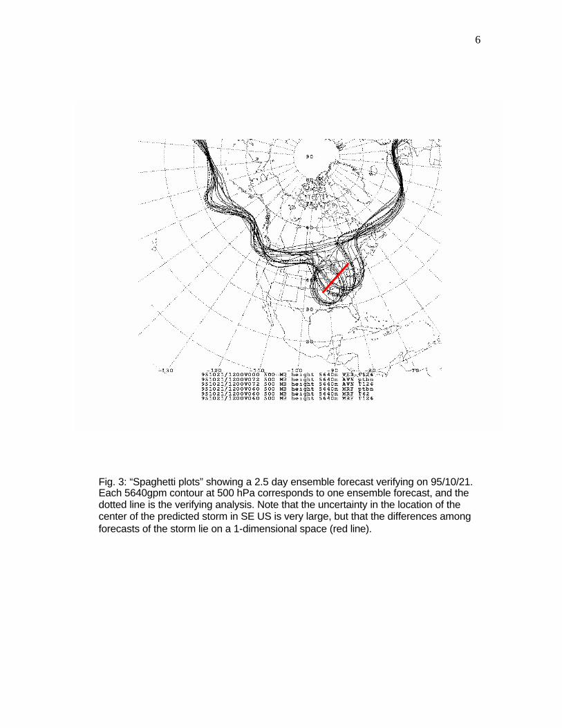
1993, 1997). Bred Vectors (like the leading Lyapunov Vectors) are independent of the norm and represent the shapes of the instabilities growing upon the evolving flow. In areas where the evolving flow is very unstable (and where forecast errors grow fast), the BVs tend to align themselves along very low dimensional subspaces (the locally most unstable perturbations, Patil et al, 2001). An example of such situation is shown in Figs. 3, where the forecast uncertainty in a 2.5 day forecast of a storm is very large, but the subspace of the ensemble uncertainty lies within a one-dimensional space. In this extreme (but not uncommon) case, a single observation at 500hPa would be able to identify the best solution! The bred vectors are the differences between the forecasts (the forecast perturbations). In unstable areas of fast growth, they tend to have shapes that are independent of the forecast length or the norm, and depend only on the verification time. This suggests that forecast errors, to the extent that they reflect instabilities of the background flow, should have shapes similar to bred vectors, and this has been confirmed with model simulations (Corazza et al, 2002). NCEP implemented an ensemble system based on breeding in 1992. Later, the US Navy, the National Centre for Medium Range Weather Forecasting in India, and the South African Meteorological Weather Service implemented similar ensemble forecasting systems. The Japanese Meteorological Agency ensemble forecasting system is also based on breeding, but imposing a partial global orthogonalization among the bred vectors, thus reducing the tendency of the bred vectors to converge towards a low dimensional space of the most unstable directions (Kyouda and Kusunoki, 2002).

6

Fig. 3: “Spaghetti plots” showing a 2.5 day ensemble forecast verifying on 95/10/21. Each 5640gpm contour at 500 hPa corresponds to one ensemble forecast, and the dotted line is the verifying analysis. Note that the uncertainty in the location of the center of the predicted storm in SE US is very large, but that the differences among forecasts of the storm lie on a 1-dimensional space (red line).

7

c. Multiple data assimilation systems Houtekamer et al (1996) developed a system based on running an ensemble of data assimilation systems using perturbed observations, implemented in the Canadian Weather Service. Hamill et al (2000) showed that in a quasi-geostrophic system, a multiple data assimilation system performs better than the singular vectors and the breeding approaches. With respect to the computational cost, the multiple data assimilation system and the singular vector approach are comparable, whereas breeding is essentially cost-free. d. Perturbed physical

parameterizations

The methods discussed above only include perturbations in the initial conditions, assuming that the error growth due to model deficiencies is small compared to that due to unstable growth of initial errors. In addition, several groups have introduced changes in the physical parameter-izations to allow for the inclusion of model uncertainty (Houtekamer et al, 1996, Stensrud et al, 2000). Buizza et al (1999) developed a perturbation approach that introduces a stochastic perturbation of the impact of subgrid scale physical parameterizations by simply multiplying the time derivative of the “physics” by a random number normally distributed with mean 1 and standard deviation 0.2. e. Multiple system ensembles Both the perturbations of the initial conditions and of the subgrid scale physical parameterizations have been shown to be successful towards

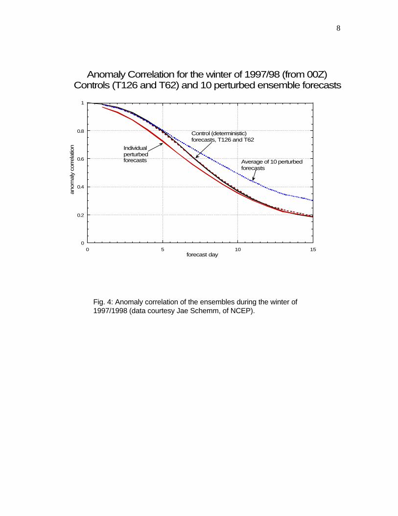
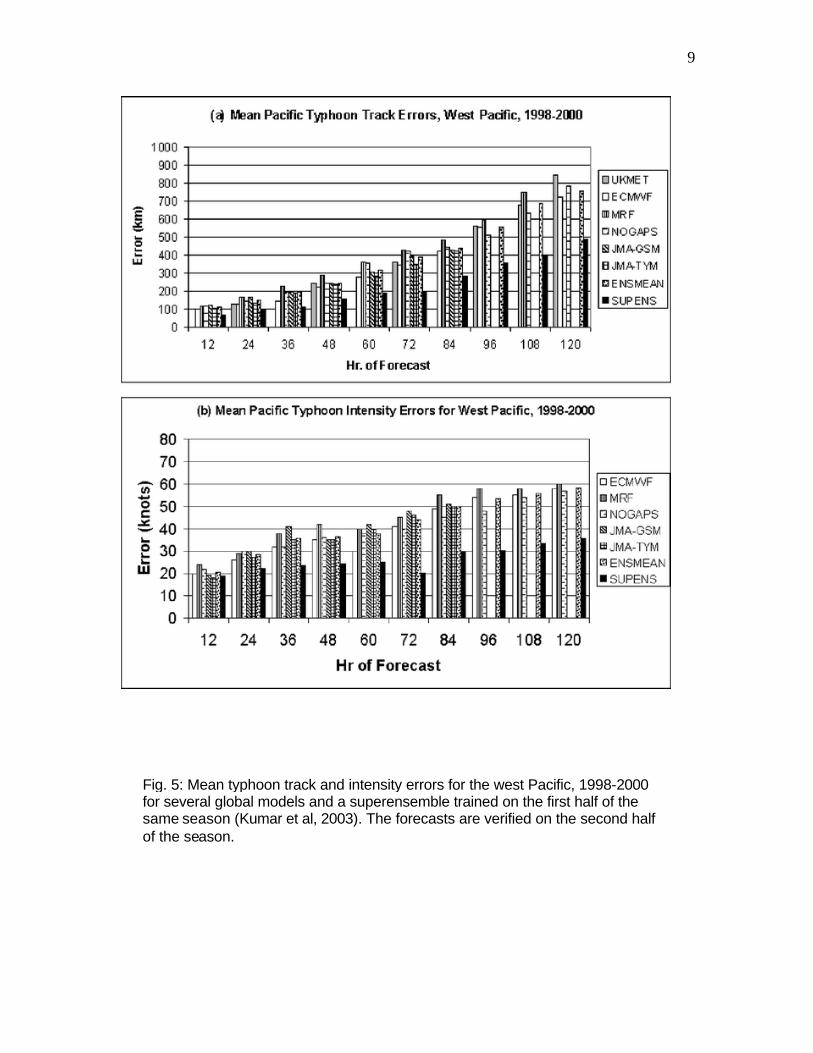
achieving the goals of ensemble forecasting. However, since they both introduce perturbations in the best estimate of the initial conditions and the model, which are in the control forecast, it can be expected that the individual perturbed forecasts should be worse than the control. A typical ensemble average for a season (Figure 4) shows that, indeed, the individual perturbed forecasts have less skill than the unperturbed control. Nevertheless, the ensemble average is an improvement over the control, especially after the perturbations grow into a nonlinear regime that tends to filter out some of the errors. An alternative to the introduction of perturbations is the use of multiple systems developed independently at different centers. In principle, an ensemble of forecasts from different operational or research centers, each aiming to be the best and choosing different competitive approaches, should sample well the uncertainty in our knowledge of both the models and the initial conditions. It has long been known that the ensemble average of multiple center forecasts is significantly better than even the best individual forecasting system (e.g., Kalnay and Ham, 1989, Fritsch et al, 2000, Arribas et al, 2004). This has also been shown to be true for regional models (Hou et al, 2001). Krishnamurti (1999) introduced the concept of “superensemble”, using linear regression and past forecasts of different systems as predictors to minimize the ensemble average prediction errors. This results in remarkable forecast improvements (e.g., Fig. 5). This method is also called “poor person’s” method to reflect that it does not require running a forecasting system.

8

0

0.2

0.4

0.6

0.8

1

0 5 10 15

Anomaly Correlation for the winter of 1997/98 (from 00Z)Controls (T126 and T62) and 10 perturbed ensemble forecasts

forecast day

Average of 10 perturbed forecasts

Individualperturbed forecasts

Control (deterministic)forecasts, T126 and T62

anom

aly

correl

atio

n

Fig. 4: Anomaly correlation of the ensembles during the winter of 1997/1998 (data courtesy Jae Schemm, of NCEP).

9

Fig. 5: Mean typhoon track and intensity errors for the west Pacific, 1998-2000 for several global models and a superensemble trained on the first half of the same season (Kumar et al, 2003). The forecasts are verified on the second half of the season.

10

f. Other methods

This field is changing quickly, and improvements and changes to the operational systems are under development. For example, ECMWF has implemented changes in the length of the optimization period for the SVs, a combination of initial and final or evolved SVs (which are more similar to BVs), and the introduction of a stochastic element in the physical parameterizations, all of which contributed to improvements in the ensemble performance. NCEP is considering the implementation of the Ensemble Transform Kalman Filter (Bishop et al, 2001) to replace breeding (see also section 3). A recent comparison of the ensemble performance of the Canadian, US and ECMWF systems (Toth et al., 2004) suggests that the ECMWF ensembles based on singular vectors behave well beyond the optimization period, at which time the model advantages of the ECMWF system are also paramount. The NCEP bred vectors are better at shorter ranges, and the multiple analyses Canadian method also seems to perform well. 3. Ensemble Kalman Filtering for

data assimilation and ensemble forecasting.

As indicated before (e.g., Ehrendorfer and Tribbia, 1997), “perfect” initial perturbations for ensemble forecasting should sample well the analysis errors. The ideal initial perturbations iδ x should have a covariance that represents the analysis error covarianceA :

1

11

KT

i iiK

δ δ=

≈− ∑ x x A (1.1).

Until recently, the problem has been that we do not know A , which changes substantially from day to day and from region to region due to instabilities of the background flow. These instabilities, associated with the “errors of the day”, are not taken into account in data assimilation systems, except for 4D-Var and Kalman Filtering, methods that are computationally very expensive. 4D-Var has been implemented at ECMWF and at MeteoFrance (Rabier et al, 2000, Andersson et al, 2004), with some simplifications such as reducing the resolution of the analysis in order to reduce the computational cost (from ~40km in the forecast model to ~120km in the assimilation model). Versions of 4D-Var are also under development in other centers. The original formulations of Kalman Filtering (Kalman, 1960) and Extended Kalman Filtering (Ghil and Malanotte-Rizzoli, 1991, Cohn, 1997) are prohibitive in practice because they would require the equivalent of N model integrations, where N is the number of degrees of freedom (d.o.f.) of the model, which is of the order of a 10^6 or more. Considerable work has been done on finding simplifying assumptions to reduce the cost of KF (e.g., Fisher, 1998, Fisher et al, 2003), but so far they have been successful only under special circumstances. Ensemble Kalman Filtering (EnKF) was introduced by Evensen (1994) as a more efficient approach to Kalman Filtering. Recent developments suggest that in the near future it will be feasible to determine simultaneously the covariance matrix A and the ideal perturbations iδ x . These methods take advantage of the fact that the size of ensembles needed to represent the analysis and forecast error covariances

11

is of order O(100), much smaller than the number of degrees of freedom of the model. When EnKF is performed locally in physical space (Ott et al, 2002), the number is smaller than 100. There are two basic approaches to EnKF. In the first one (known as “perturbed observations”) an ensemble of data assimilations is carried out using the same observations to which random have been added. The ensemble is used to estimate the forecast error covariance needed in the Kalman Filter (Evensen, 1994, Houtekamer and Mitchell, 1998, Hamill and Snyder, 2000). This approach has already been shown to be very competitive with the operational 3D-Var, an important milestone, given that 3D-Var has the benefit of years of improved developments (Houtekamer et al, 2004). The second approach is the class of square root filters (Tippett et al, 2002), and does not require perturbing the observations. Several groups have recently independently developed square root filters (Bishop et al, 2001, Anderson, 2001, Whitaker and Hamill, 2002, Ott et al, 2002). The ensemble forecasts are used to obtain a background error covariance at the time of the analysis. The full Kalman Filter equations and the new observations are then used to obtain the analysis increment (difference between the analysis and the forecast) and the analysis error covariance, all lying within the subspace of the forecast ensemble. After this is completed, the new initial analysis perturbations iδ x are obtained by solving the square root problem of equation (1.1), and the analysis cycle can continue. Several of the Ensemble Kalman Filters further reduce the computational cost by assimilating the observations one at a time, for the whole physical domain, a

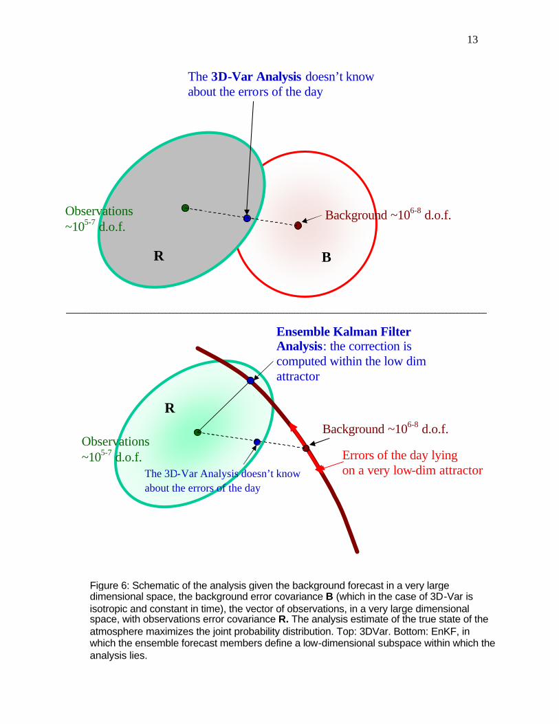
method known as sequential assimilation of observations. This is done using a localization of the error covariance in the horizontal and in the vertical, to avoid spurious long-distance correlations due to sampling. In the Local Ensemble Kalman Filter (LEKF) method (Ott et al, 2002, 2004, Szunyogh et al, 2004a, b), the Ensemble Kalman Filter problem is solved locally in physical space. For each grid point a local 3D volume of the order of 1000km by 1000km and a few vertical layers is used to perform the analysis. The Kalman Filter equations are solved exactly on this subspace locally spanned by the global ensemble members, using all the observations available within the volume. This localization in space results in a further reduction of the number of necessary ensemble members, so that matrix operations are done in a very low dimensional space. The analysis is carried out independently at each grid point, with essentially perfectly parallel computations. In order to visualize the main advantage of Ensemble Kalman Filtering (EnKF), we compare it with the 3D-Var approach currently operational in most centers, in which the analysis error covariance is estimated as an average over many cases. The top schematic Fig. 6 shows how the 3D-Var analysis maximizes the joint probability defined by the observations error covariance and the background error covariance, but does not know about “errors of the day”. The bottom schematic shows how in the EnKF, the ensemble perturbations defines a low-dimensional subspace (10-100), and the KF analysis maximizes the joint probability within this subspace. Because all the computations are performed within this subspace, the rank of the matrices involved is low, and the Kalman Filter equations providing the analysis and

12

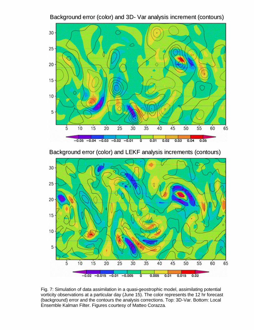
analysis error covariance are solved directly, not iteratively. Fig. 7 shows an example of EnKF and 3D-Var using a quasi-geostrophic data assimilation system (Morss et al, 2000, Hamill and Snyder, 2000, Corazza et al, 2002). The colors show the background (12 hour forecast) errors and the contours are the analysis corrections based on a given set of observations. The top panel corresponds to 3D-Var, using a background error covariance constant in time. Since the system does not know about the “errors of the day”, the corrections brought by the new observations tend to be isotropic. The bottom panel shows that the Local Ensemble Kalman Filter (Ott et al, 2004, Szunyogh et al, 2004b) is much more efficient in correcting the background errors with the same observations. The large improvements that the LEKF makes on the analysis are also apparent in the 3-day forecasts (not shown). Performing the EnKF locally in space substantially reduces the number of ensemble members required for the

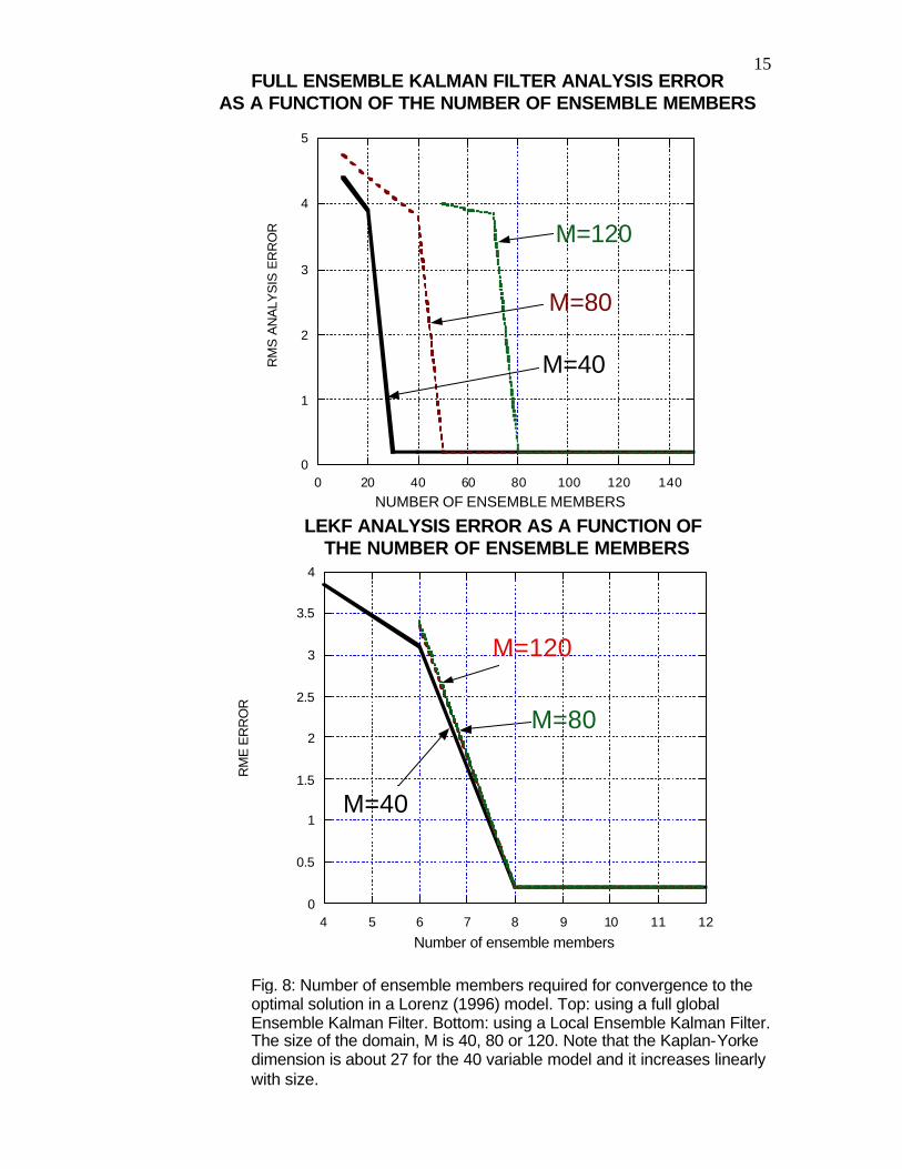
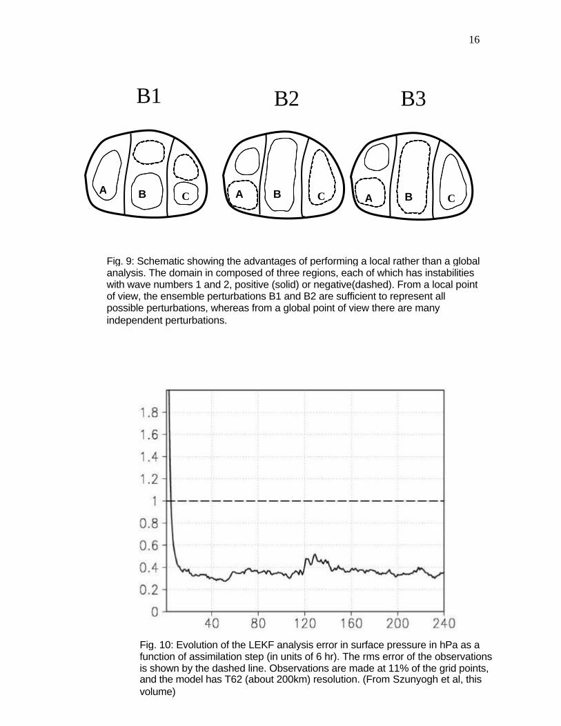
analysis, as shown with experiments done with the Lorenz (1996) model (Fig. 8, from Ott et al, 2004). When performed globally, the number of ensemble members required for the EnKF to converge is proportional to the size of the model. When done locally, the number of ensemble members is reduced from 27 to 8, and does not increase with the size of the model. In addition, the analysis for different grid points can be carried out in parallel, since they are independent from each other. The advantage of a local analysis in reducing the size of the required ensemble is illustrated in Fig. 9, showing a schematic of an ensemble with three independent unstable regions. In each of the regions wave number 1 and 2 are unstable. This situation is reminiscent of the global atmosphere, containing regions where baroclinic instabilities can develop independently. From a local point of view, the first two perturbations are enough to represent all possible combinations of instabilities, whereas from a global point of view, the third perturbation and many others are linearly independent.

13

Background ~106-8 d.o.f.

The 3D-Var Analysis doesn’t know about the errors of the day

Observations ~105-7 d.o.f.

B R

Background ~106-8 d.o.f. Observations ~105-7 d.o.f.

The 3D-Var Analysis doesn’t know about the errors of the day

Errors of the day lying on a very low-dim attractor

Ensemble Kalman Filter Analysis: the correction is computed within the low dim attractor

Figure 6: Schematic of the analysis given the background forecast in a very large dimensional space, the background error covariance B (which in the case of 3D-Var is isotropic and constant in time), the vector of observations, in a very large dimensional space, with observations error covariance R. The analysis estimate of the true state of the atmosphere maximizes the joint probability distribution. Top: 3DVar. Bottom: EnKF, in which the ensemble forecast members define a low-dimensional subspace within which the analysis lies.

R

14

Fig. 7: Simulation of data assimilation in a quasi-geostrophic model, assimilating potential vorticity observations at a particular day (June 15). The color represents the 12 hr forecast (background) error and the contours the analysis corrections. Top: 3D-Var. Bottom: Local Ensemble Kalman Filter. Figures courtesy of Matteo Corazza.

BBaacckkggrroouunndd eerrrroorr ((ccoolloorr)) aanndd 33DD-- VVaarr aannaallyyssiiss iinnccrreemmeenntt ((ccoonnttoouurrss))

BBaacckkggrroouunndd eerrrroorr ((ccoolloorr)) aanndd LLEEKKFF aannaallyyssiiss iinnccrreemmeennttss ((ccoonnttoouurrss))

15

0

1

2

3

4

5

0 20 40 60 80 100 120 140

FULL ENSEMBLE KALMAN FILTER ANALYSIS ERRORAS A FUNCTION OF THE NUMBER OF ENSEMBLE MEMBERS

RM

S A

NA

LYS

IS E

RR

OR

NUMBER OF ENSEMBLE MEMBERS

M=40

M=80

M=120

0

0.5

1

1.5

2

2.5

3

3.5

4

4 5 6 7 8 9 10 11 12

LEKF ANALYSIS ERROR AS A FUNCTION OF THE NUMBER OF ENSEMBLE MEMBERS

RM

E E

RR

OR

Number of ensemble members

M=40

M=80

M=120

Fig. 8: Number of ensemble members required for convergence to the optimal solution in a Lorenz (1996) model. Top: using a full global Ensemble Kalman Filter. Bottom: using a Local Ensemble Kalman Filter. The size of the domain, M is 40, 80 or 120. Note that the Kaplan-Yorke dimension is about 27 for the 40 variable model and it increases linearly with size.

16

Fig. 9: Schematic showing the advantages of performing a local rather than a global analysis. The domain in composed of three regions, each of which has instabilities with wave numbers 1 and 2, positive (solid) or negative(dashed). From a local point of view, the ensemble perturbations B1 and B2 are sufficient to represent all possible perturbations, whereas from a global point of view there are many independent perturbations.

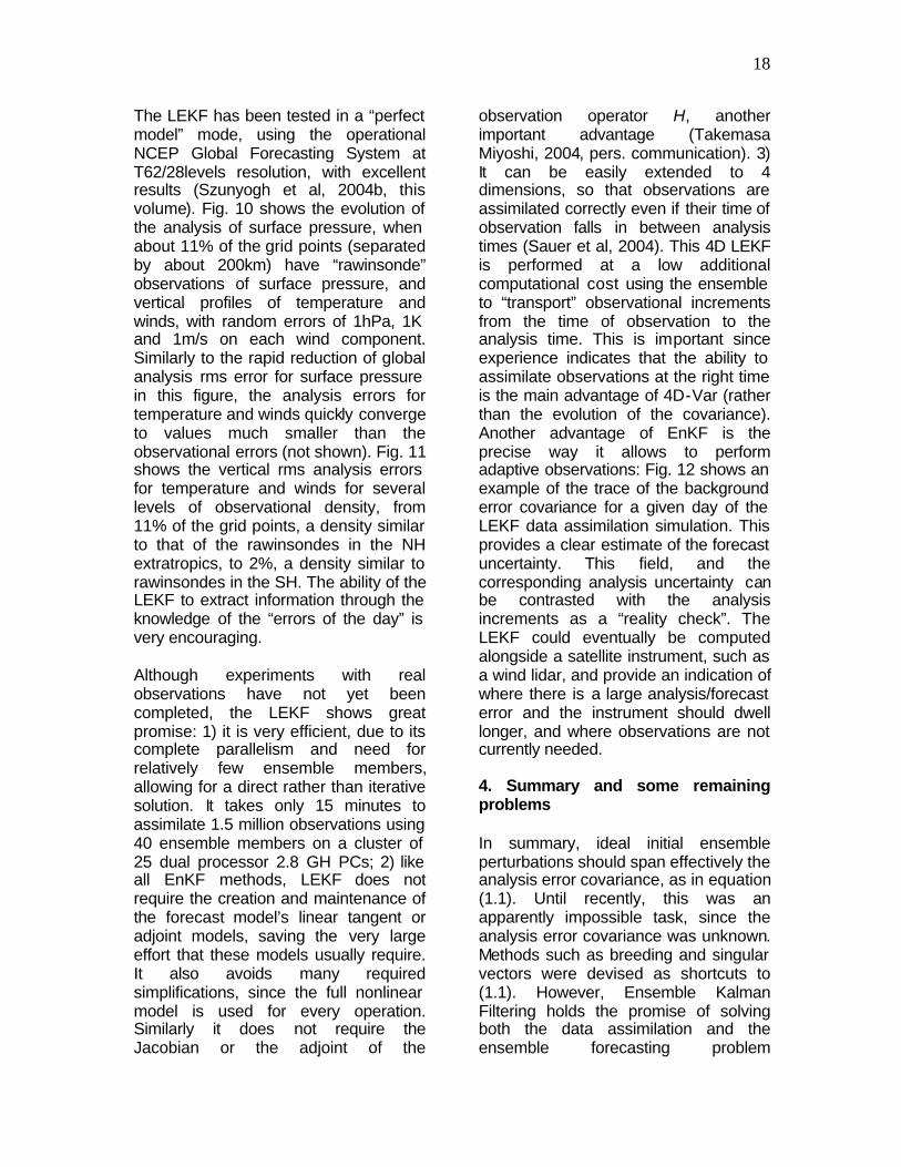
Fig. 10: Evolution of the LEKF analysis error in surface pressure in hPa as a function of assimilation step (in units of 6 hr). The rms error of the observations is shown by the dashed line. Observations are made at 11% of the grid points, and the model has T62 (about 200km) resolution. (From Szunyogh et al, this volume)

A C B C B C B A A

B 1 B 2

B3

17

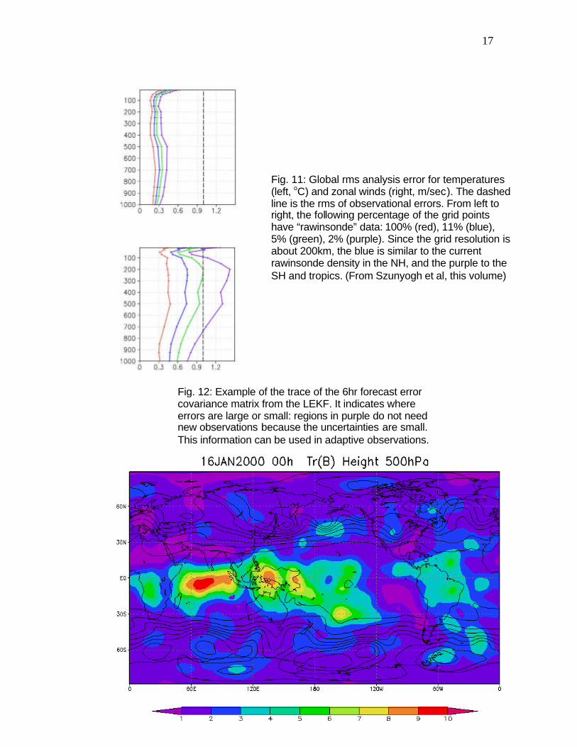
Fig. 11: Global rms analysis error for temperatures (left, oC) and zonal winds (right, m/sec). The dashed line is the rms of observational errors. From left to right, the following percentage of the grid points have “rawinsonde” data: 100% (red), 11% (blue), 5% (green), 2% (purple). Since the grid resolution is about 200km, the blue is similar to the current rawinsonde density in the NH, and the purple to the SH and tropics. (From Szunyogh et al, this volume)

Fig. 12: Example of the trace of the 6hr forecast error covariance matrix from the LEKF. It indicates where errors are large or small: regions in purple do not need new observations because the uncertainties are small. This information can be used in adaptive observations.

18

The LEKF has been tested in a “perfect model” mode, using the operational NCEP Global Forecasting System at T62/28levels resolution, with excellent results (Szunyogh et al, 2004b, this volume). Fig. 10 shows the evolution of the analysis of surface pressure, when about 11% of the grid points (separated by about 200km) have “rawinsonde” observations of surface pressure, and vertical profiles of temperature and winds, with random errors of 1hPa, 1K and 1m/s on each wind component. Similarly to the rapid reduction of global analysis rms error for surface pressure in this figure, the analysis errors for temperature and winds quickly converge to values much smaller than the observational errors (not shown). Fig. 11 shows the vertical rms analysis errors for temperature and winds for several levels of observational density, from 11% of the grid points, a density similar to that of the rawinsondes in the NH extratropics, to 2%, a density similar to rawinsondes in the SH. The ability of the LEKF to extract information through the knowledge of the “errors of the day” is very encouraging. Although experiments with real observations have not yet been completed, the LEKF shows great promise: 1) it is very efficient, due to its complete parallelism and need for relatively few ensemble members, allowing for a direct rather than iterative solution. It takes only 15 minutes to assimilate 1.5 million observations using 40 ensemble members on a cluster of 25 dual processor 2.8 GH PCs; 2) like all EnKF methods, LEKF does not require the creation and maintenance of the forecast model’s linear tangent or adjoint models, saving the very large effort that these models usually require. It also avoids many required simplifications, since the full nonlinear model is used for every operation. Similarly it does not require the Jacobian or the adjoint of the

observation operator H, another important advantage (Takemasa Miyoshi, 2004, pers. communication). 3) It can be easily extended to 4 dimensions, so that observations are assimilated correctly even if their time of observation falls in between analysis times (Sauer et al, 2004). This 4D LEKF is performed at a low additional computational cost using the ensemble to “transport” observational increments from the time of observation to the analysis time. This is important since experience indicates that the ability to assimilate observations at the right time is the main advantage of 4D-Var (rather than the evolution of the covariance). Another advantage of EnKF is the precise way it allows to perform adaptive observations: Fig. 12 shows an example of the trace of the background error covariance for a given day of the LEKF data assimilation simulation. This provides a clear estimate of the forecast uncertainty. This field, and the corresponding analysis uncertainty can be contrasted with the analysis increments as a “reality check”. The LEKF could eventually be computed alongside a satellite instrument, such as a wind lidar, and provide an indication of where there is a large analysis/forecast error and the instrument should dwell longer, and where observations are not currently needed. 4. Summary and some remaining problems In summary, ideal initial ensemble perturbations should span effectively the analysis error covariance, as in equation (1.1). Until recently, this was an apparently impossible task, since the analysis error covariance was unknown. Methods such as breeding and singular vectors were devised as shortcuts to (1.1). However, Ensemble Kalman Filtering holds the promise of solving both the data assimilation and the ensemble forecasting problem

19

simultaneously, since both the lhs and the rhs of this equation are obtained during the EnKF assimilation. Furthermore, experience with the NCEP global model indicates that it is possible to carry out this advanced approach with present day supercomputers and without sacrificing the resolution of the analysis model. Additional advantages are that the linear tangent and adjoints codes of the forecast model or the observation operators are not needed, and that atmospheric data can be assimilated at the time they were observed. One of the most important remaining problems is that of model deficiencies, leading to bias in data assimilation (Dee and DaSilva, 1999), to systematic forecast errors, and to ensemble deficiencies such as indicated in Fig. 1b. Obviously, the ultimate solution to this problem lies in the improvement of the models (e.g., Simmons and Hollingsworth, 2002), but until that stage is reached, empirical approaches may be needed. A successful approach to start addressing the problem of errors and uncertainties in the model is the use of multiple models (Krishnamurti 1999, Hou et al, 2001, Fritsch, 2001, Kalnay and Ham, 1989). Other approaches (DelSole and Hou, 1999, Kaas et al, 1999) rely on empirical statistical methods to modify the model and reduce forecast errors. In another method, known as “dressing”, random perturbations are added to the ensemble forecasts in order to reproduce the observed error covariance with an enhanced ensemble forecast spread (Roulston and Smith, 2003, Wang and Bishop, 2004). It is possible that the Ensemble Kalman Filtering approach will also be able to efficiently minimize model errors by augmenting the space of model

variables with a relatively small number of parameters associated with model errors, and using the observations to estimate the optimal value of their time-varying coefficients (e.g., Anderson, 2001). Another important problem in ensemble forecasting and data assimilation arises with the presence of coupled instabilities with a wide range of time scales. For example, atmospheric convection, baroclinic instabilities, and the ENSO instabilities of the coupled ocean-atmosphere system are characterized by time scales of minutes, days and months respectively. This difficult problem of coupled systems (Timmerman, 2002) has been attacked by allowing fast, small amplitude modes to saturate (Toth and Kalnay, 1993, Aurell et al, 1996, Boffetta et al, 1998). Toth and Kalnay (1993, 1996) proposed that breeding with rescaling amplitudes above the saturation level could be used to filter fast, small amplitude instabilities such as convection, without the need to eliminate or simplify their physical impact. Conversely, the choice of very small amplitudes for the rescaling can identify the bred vectors dominated by convection. This conjecture was validated by Lorenz (1996), and Peña and Kalnay (2004). Unfortunately, In the case of the coupled ocean-atmosphere system, the “atmospheric weather noise” has larger, not smaller amplitudes than the slow ENSO signals. Peña and Kalnay (2004) have shown that in this case one can still take advantage of the longer time scale of the slow modes. Breeding with rescaling at longer intervals can identify the slower coupled mode (unlike linear singular vectors or Lyapunov vectors, which are linear, and select the fastest mode). Cai et al (2002) performed breeding with the Cane-Zebiak model

20

and used the bred vectors for simulated ensemble forecasting and data assimilation experiments, with very encouraging results. Yang et al (2004) also obtained good results using the operational NAS NSIPP coupled GCM, and very similar results were obtained with an NCEP coupled GCM. These “perfect model” breeding experiments were done using a rescaling interval of one month and the Niño-3 SST anomalies as the rescaling norm. Results with the operational NSIPP coupled data assimilation system indicate that the growth rate and shape of coupled bred vectors in the Equatorial region is strongly related to the ENSO forecast error. These results suggest that in coupled systems that contain fast and slow instabilities, it may not be possible to use the same EnKF approach to do data assimilation for both the fast and the slow processes. As in breeding, it may be necessary to choose different time intervals for the analysis of fast and slow instabilities. 5. Acknowledgements This work was supported by the W. M. Keck Foundation, by the NPOESS Integrated Program, and by the NOAA Office of Global Programs. I have been very fortunate to collaborate and learn with the members of the Chaos Group at the University of Maryland, Ming Cai and Zoltan Toth, and students (Matteo Corazza, Shu-Chih Yang, Malaquias Pena and Takemasa Miyoshi). 6. References Ahlquist, Jon, 2000: Almost Anything can be a Singular Vector. www.met.fsu.edu/ftp/ahlquist/singvect.ps

Anderson, J. L., 2001: An ensemble adjustment filter for data assimilation. Mon. Wea. Rev., 129, 2884-2903. Andersson, E, C. Cardinali, M. Fisher, E. Hólm, L. Isaksen, Y. Trémolet and A. Hollingsworth, 2004: Developments in ECMWF’s 4d-Var system. Paper J.1. AMS preprints of the 20th Conference on Weather Analysis and Forecasting/16th Conference on Numerical Weather Prediction. Arribas, A.; Robertson, KB; Mylne, KR, 2004: Test of a poor man's ensemble prediction system for short-range probability forecasting. Submitted Aurell E., Boffetta G., Crisanti A., Paladin G. and Vulpinai A., 1996: Predictability in systems with many degrees of freedom. Phys. Rev. E, 52, 2337. Bishop, C. H., B. J. Etherton and S. J. Majumdar, 2001: Adaptive sampling with the ensemble transform Kalman filter. Part I: Theoretical aspects. Mon. Wea. Rev., 129, 420-436. Boffetta G., Crisanti A., Paparella F., Provenzale A. and Vulpiani A.,1998: Slow and fast dynamics in coupled systems: A time series analysis view. Physica D 116, 301-312. Buizza, R., 1997: Potential forecast skill of ensemble prediction, and spread and skill distributions of the ECMWF Ensemble Prediction System. Mon. Wea. Rev., 125, 99-119. Buizza, R., Petroliagis, T., Palmer, T.N., Barkmeijer, J.,Hamrud, M., Hollingsworth, A., Simmons, A., and Wedi, N., 1998: Impact of model resolution and ensemble size on the performance of an ensemble prediction system.Q.J.R. Meteorol. Soc., 124, 1935-1960.

21

Buizza, R., Miller, M., and Palmer, T.N., 1999: Stochastic simulation of model uncertainties. Q.J.R. Meteorol. Soc., 125, 2887-2908. Buizza, R., Barkmeijer, J., Palmer, T.N.,and Richardson, D.S., 2000: Current status and future developments of the ECMWF Ensemble Prediction System. Meteorol.Appl., 7, 163-175. Cai, M., E. Kalnay, Z. Toth, 2003: Bred Vectors of the Zebiak-Cane Model and Their Application to ENSO Predictions. J. Climate, 16, 40-56. Cohn, S. E., 1997: An introduction to estimation theory. J. Meteor. Soc. Japan, 75 (1B), 257-288. Cohn, S. E., and R. Todling., 1996: Approximate data assimilation schemes for stable and unstable dynamics. J. Met. Soc. Japan, 74, 63-75. Corazza, M., E. Kalnay, D. J. Patil, R. Morss, I. Szunyogh, B. R. Hunt, E. Ott, and M. Cai, 2003: Use of the breeding technique to estimate the structure of the analysis “errors of the day”. Nonlinear Processes in Geophysics, 10, 233-243. Dee, Dick P., Arlindo M. da Silva, 1999: Maximum-Likelihood Estimation of Forecast and Observation Error Covariance Parameters. Part I: Methodology. Mon. Wea. Rev., 127, 1822-1834. DelSole, T., and A. Y. Hou, 1999: Empirical Correction of a Dynamical Model. Part I: Fundamental Issues. Mon. Wea. Rev., 127, 2533-2545. Ebisuzaki, W., and E Kalnay., 1991: Ensemble experiments with a new lagged average forecasting scheme. WMO, Research activities in atmospheric and oceanic modeling. Report #15, pp6.31-6.32. [Available

from WMO, C.P. No 2300, CH1211, Geneva, Switzerland]. See also Kalnay (2003), p. 234. Ehrendorfer, M. and J. J. Tribbia., 1997: Optimal prediction of forecast error covariances through singular vectors. J. Atmos. Sci., 54, 286-313. Ehrendorfer, M., 2003: The Liouville Equation in Atmospheric Predictability. In: Proceedings ECMWF Seminar on Predictability of Weather and Climate, 9 – 13 September 2002, pp. 47-81. Errico, R and D. Baumhefner, 1987: Predictability experiments using a high resolution limited area model. Mon.. Wea. Rev. 115, 488-504. Epstein, E. S., 1969: Stochastic -dynamic prediction. Tellus, 21, 739-759. Evensen, G., 1994: Sequential data assimilation with a nonlinear quasigeostrophic model using Monte carlo methods to forecast error statistics. J. Geophys. Res. 99 (C5), 10143-10162. Fisher, M, 1998: Development of a simplified Kalman Filter. ECMWF Tech Memo 260. 16pp. Fisher, M., L. Isaksen, M. Ehrendorfer, A. Beck and E. Andersson, 2003: A critical evaluation of the reduced-rank Kalman filter (RRKF) approach to flow-dependent cycling of background error covariances. ECMWF Tech. Memo. Fritsch, J. M., J. Hilliker, J. Ross, R. L. Vislocky., 2000: Model Consensus. Wea. Forecasting, 15, 571–582. Ghil, M. and Malanotte-Rizzoli., 1991: Data Assimilation in meteorology and oceanography. Adv. Geophys., 33, 141-266

22

Hamill, Thomas M., Chris Snyder, Rebecca E. Morss., 2000: A Comparison of Probabilistic Forecasts from Bred, Singular-Vector, and Perturbed Observation Ensembles. Mon. Wea. Rev., 128, 1835-1851. Hamill, Thomas M., Chris Snyder., 2000b: A Hybrid Ensemble Kalman Filter-3D Variational Analysis Scheme. Mon. Wea. Rev., 128, 2905-2919. Hoffman, R. N. and E. Kalnay., 1983: Lagged Average Forecasting, and Alternative to Monte Carlo Forecasting. Tellus, 35A, 100-118. Hollingsworth, A., 1980: An experiment in Monte Carlo forecasting. Workshop on Stochastic-Dynamic Forecasting. ECMWF, Shinfield Park, reading, UK, RG2 9AX, 65-85. Hou, D., E. Kalnay, and K.K. Droegemeier., 2001: Objective verification of the SAMEX '98 ensemble forecasts. Mon. Wea. Rev., 129, 73-91. Houtekamer, P.L., L. Lefaivre and J. Derome, 1996: A system simulation approach to ensemble prediction. Mon. Wea. Rev., 124, 1225-1242. Houtekamer, P. L., and H. L. Mitchell., 1998: Data assimilation using an ensemble Kalman filter technique. Mon. Wea. Rev., 126, 796-811. Houtekamer, Peter L., Herschel L. Mitchell, Gérard Pellerin, Mark Buehner, Martin Charron, Lubos Spacek, and Bjarne Hansen, 2004: Atmospheric data assimilation with the ensemble Kalman filter: Results with real observations. Monthly Weather Review , under review. Hunt, B.R., E. Kalnay, E.J. Kostelich, E. Ott, D.J. Patil, T. Sauer, I. Szunyogh, J.A. Yorke, A.V. Zimin, 2003: Four Dimensional Ensemble Kalman Filtering. Tellus, in print.

Kaas, E., A. Guldberg, W. May and M. Decque., 1999: Using tendency errors to tune the parameterization of unresolved dynamical scale interactions in atmospheric general circulation models. Tellus, 51A, 612-629. Kalman, R., 1960: A new approach to linear filtering and prediction problems, Trans. ASME, Ser. D, J. Basic Eng. 82: 35-45. Kalnay, Eugenia and M. Ham., 1989: Forecasting forecast skill in the Southern Hemisphere. Preprints of the 3rd International Conference on Southern Hemisphere Meteorology and Oceanography, Buenos Aires , 13-17 November 1989. Boston, MA: Amer. Meteor. Soc. Kalnay, E, 2003: Atmospheric modeling, datq assimilation and predictability. Cambridge University Press, 341 pp. Krishnamurti, TN, 1999: Improved weather and seasonal climate forecasts from multimodel superensemble. Science 285, 1548-1550. Kyouda, M. and S. Kusunoki, 2002: Ensemble Prediction System. Outline of the Operational Numerical Weather Prediction at the Japan Meteorological Agency. JMA, 59-63. Leith, C. E., 1974: Theoretical skill of Monte Carlo forecasts. Mon. Wea. Rev., 102, 409-418. Lorenz, E. N., 1963: Deterministic nonperiodic flow. J. Atmos. Sci., 20, 130-141. Lorenz, E. N., 1965: A study of the predictability of a 28-variable atmospheric model. Tellus, 17, 321-333. Lorenz, E. N., 1996: Predictability- A problem partly solved. Proceedings of

23

the ECMMWF Seminar on Predictability. September 4-8, 1995, Reading, England, Vol 1, 1-18. Molteni, F. and T. N. Palmer, 1993: Predictability and finite-time instability of the northern winter circulation. Q. J. Meteorol. Soc., 119, 269-298. Molteni, F., R. Buizza, T. N. Palmer, and T. Petroliagis, 1996: The ECMWF ensemble prediction system: Methodology and validation. Quart. J. Roy. Meteor. Soc., 122, 73-119. Morss, R. E., 1999: Adaptative observations: Idealized sampling strategies for improving numerical weather prediction., Ph. D. thesis, Massachusetts Institute of Technology, 225 pp. Ott, E., B. R. Hunt, I. Szunyogh, M. Corazza, E.Kalnay, D. J. Patil, J. A. Yorke, A. V. Zimin, and E. Kostelich, 2002: Exploiting local low dimensionality of the atmospheric dynamics for efficient Kalman filtering. http://arxiv.org/abs/physics/0203058. Ott, E., B. R. Hunt, I. Szunyogh, A.V. Zimin, E.J. Kostelich, M. Corazza, E. Kalnay, D.J. Patil, J.A. Yorke, 2002: A local ensemble Kalman filter for atmospheric data assimilation. Tellus, in press. Palmer, T. N., R. Gelaro, J. Barkmeijer and R. Buizza., 1998: Singular vectors, metrics and adaptive observations. J. Atmos. Sci, 55, 633-653. Patil, D. J. S., B. R. Hunt, E. Kalnay, J. A. Yorke, and E. Ott., 2001: Local Low Dimensionality of Atmospheric Dynamics. Phys. Rev. Lett., 86, 5878. Peña, Malaquias and Eugenia Kalnay, 2004: Separating fast and slow modes in coupled chaotic systems. Nonlinear Processes in Physics, in press.

Rabier, F., H. Järvinen, E. Klinker, J.F. Mahfouf and A. Simmons, 2000: The ECMWF operational implementation of four dimensional variational assimilation. Part I: experimental results with simplified physics. Q. J. R. Meteorol. Soc. 126, 1143—1170. Roulston, M. S. and L. A. Smith, 2003: Combining dynamical and statistical ensembles. Tellus, 55A, 16-30. Sauer, T., B. R. Hunt, J. A. Yorke, A. V. Zimin, E., Ott, E. J. Kostelich, I., Szunyogh, G. Gyarmati, E. Kalnay, D. J. Patil, 2004a: 4D Ensemble Kalman filtering for assimilation of asynchronous observations. Paper J5.4 in AMS preprints of the 20th Conference on Weather Analysis and Forecasting/16th Conference on Numerical Weather Prediction. Simmons, A. J. and A. Hollingsworth, 2002: Some aspects of the improvement in skill of numerical weather prediction. Q. J. R. Meteorol. Soc., 128, 647—678. Stensrud, D. J., J.-W. Bao, and T. T. Warner, 2000: Using initial condition and model physics perturbations in short-range ensembles. Mon. Wea. Rev., 128, 2077–2107. Szunyogh, Istvan, Eric J. Kostelich, Gyorgyi Gyarmati, Brian R. Hunt, Edward Ott, Aleksey V. Zimin, Eugenia Kalnay, Dhanurjay Patil, and James A. Yorke, 2004a: A Local Ensemble Kalman Filter for the NCEP GFS Model. Paper J2.4 in AMS preprints of the 20th Conference on Weather Analysis and Forecasting/16th Conference on Numerical Weather Prediction. Seattle, Washington, 11-15 January 2004 Szunyogh, Istvan, Eric J. Kostelich, Gyorgyi Gyarmati, Brian R. Hunt, Edward Ott, Eugenia Kalnay, Dhanurjay Patil, and James A. Yorke, 2004b:

24

Development of the Local Ensemble Kalman Filter at the University of Maryland. Extended abstracts of the Symposium on the 50th Anniversary of Operational Numerical Weather Prediction (this volume). Timmermann, Axel, 2002: The predictability of coupled phenomena. Proceedings of the seminar on predictability of weather and climate, held at ECMWF on 9-13 September, 2002, Reading, England. Tippett, M. K., J. L. Anderson, C. H. Bishop, T. M. Hamill, and J. S. Whitaker, 2002: Ensemble square root filters. Mon. Wea. Rev., 131, 1485-1490. Toth, Z. and E. Kalnay., 1993: Ensemble forecasting at NMC: the generation of perturbations. Bull. Amer. Meteor. Soc., 74, 2317-2330. Toth, Zoltan and Eugenia Kalnay, 1996: Climate ensemble forecasts: How to create them? Idojaras, 100, 43–52. Toth, Zoltan and Eugenia Kalnay., 1997: Ensemble Forecasting at NCEP: the breeding method,. Mon. Wea. Rev., 125, 3297-3318. Toth, Z., R Buizza, and P Houtekamer, 2003: Global Ensemble Forecasting. Geophysical Research Abstracts, 5, 11374. Tracton, M. S., and E. Kalnay., 1993: Ensemble forecasting at NMC: Practical aspects. Wea. Forecasting, 8, 379-398. Wang, X., and C. H. Bishop, 2003: A comparison of breeding and ensemble transform Kalman filter ensemble forecast schemes. J. Atmos. Sci., 60,1140-1158. ? Wang, Xuguang and Craig H. Bishop, 2004: Ensemble Augmentation With A

New Dressing Kernel. AMS, Seattle, January 2004. Whitaker, J. S., and T. H. Hamill, 2002: Ensemble Data Assimilation without perturbed observations. Mon. Wea. Rev., 130, 1913-1924. Yang, Shu-Chih, Ming Cai, Malaquías Peña1, and Eugenia Kalnay, 2004: Initialization of Unstable Coupled Systems by Breeding Ensembles. Paper J13.12 in preprints of the AMS Symposium on Forecasting Weather and Climate in the Atmosphere and Oceans.