Forecasting Indoor Environment using

Ensemble-based Data Assimilation Algorithms

Cheng-Chun Lin

A Thesis

In the Department

of

Building, Civil and Environmental Engineering

Presented in Partial Fulfillment of the Requirements

for the Degree of Doctor of Philosophy at

Concordia University

Montreal, Quebec, Canada

December 2014

© Cheng-Chun Lin, 2014

iii

ABSTRACT

Forecasting Indoor Environment using Ensemble-based Data Assimilation Algorithms

Cheng-Chun, Lin, Ph.D.

Concordia University, 2014

Forecasting simulations of building environment have attracted growing interests since more and

more applications have been explored. Occupant’s thermal comfort, safety and energy efficiency

are reported to directly benefit from accurate predicted building physical conditions. Among all

available research regarding forecasting indoor environment, there are substantially fewer studies

relating to occupant safety and emergency forecasting and response than that of comfort and

energy savings. This may due to the nature that the forecasting simulations associated with life

safety concerns demand higher accuracy. Although the tasks of forecasting potential threats in

the indoor environment are especially challenging, the benefits can be significant. For example,

toxic contaminants such as carbon monoxide from fire smoke can be monitored and removed

before the concentration reaches a harmful level. The sudden release of hazardous gases or the

smoke generated from an accidental fire can also be detected and analyzed. Then, based on the

results of forecasting simulations, the building control system can provide an efficient evacuation

plan for all occupants in the building. However, by using traditional simulation tools that utilize

one set of initial inputs to forecast future physical states, the predicted physical conditions may

depart from reality as the simulation progresses over time.

iv

In this thesis, forecasting simulations of building safety management are improved by applying

the theory of data assimilation where the simulation results are aided by the sensor

measurements. Instead of studying methods that require high computational resources, this

research focuses on affordable approaches, ensemble-based algorithms, to forecast indoor

environment to solve various safety problems including forecasting indoor contaminant and

smoke transport. The resulting models are able to provide predictions with noticeable accuracy

by only using affordable computer resources such as a regular PC. Finally, a scaled compartment

fire experiment is conducted to verify the real-time predictability of the model. The results

indicate that the proposed method is able to forecast real-time fire smoke transport with

significant lead time. Overall, the method of Ensemble Kalman Filter (EnKF) is efficient to

apply to forecasting indoor contaminant and smoke transport problems. In the end of this thesis,

suggestions are summarized to help those who would like to apply EnKF to solve other building

simulation problems.

v

For the most important persons of my life,

my wife Feng-Hua and our children Yahsi and Janhsi.

vi

Acknowledgements

First, I would like to express my great thanks to my supervisor, Dr. Liangzhu (Leon) Wang, for

his patience and guidance. He is enthusiastic and dedicated in science research and even willing

to spend his weekend to help me with programming and correcting my writings.

Besides, I would like to thank the rest of my thesis committee: Dr. Fariborz Haghighat, Dr.

Samuel Li, Dr. Hoi Dick Ng and Dr. David Torvi. Their comments are a treasure to me not only

for this thesis but also for my future research.

It would also like to thank Dr. Nils van Velzen for helping me program data assimilation models.

Reading his PhD thesis is a pleasant and inspires me for building my own models.

I would also like to show my gratitude to my lab mates, Jeremy (Guanchao) Zhao and Dr. Wael

Saleh, who are very knowledgeable in fire experiments and PIV. They helped me set up whole

experiment from scratch and performing the experiments altogether. In addition, I would like to

thank Dr. Hoi Dick Ng for providing experiment equipment and a large lab space for us.

I would like to thank my mother’s understanding while I gave up my job in Taiwan in order to

catch my dream. Without her financial support, this thesis would not have been possible.

Finally, I would like to thank my wife Feng-Hua and our children Yahsi and Janhsi. Their

encouragement and support mean a lot to me. The honor is all yours!

vii

Table of Contents

Chapter 1. Introduction …………………………………………………………..………… 1

1.1 General statement of the problem …………………………….………….………… 1

1.2 Forecasting indoor environment using data assimilation ………………………….. 2

1.2.1 Development of data assimilation ….………….………….………….…………. 3

1.2.2 Categories of data assimilation algorithms ….………….………….………….... 6

1.3 General research objectives and thesis outline …………………………………..… 9

References ……………………………………………………………………………… 11

Chapter 2. Literature Reviews …………………………………………………………….. 13

2.1 Forecasting indoor environment……………………………………………………. 13

2.2 Forecasting indoor environment using data assimilation …………………………. 15

2.3 Ensemble based data assimilation algorithms ……………………….….…………. 17

2.3.1 Ensemble square root filter (EnSRF) ….………….………….………….……… 18

2.3.2 Local ensemble transform Kalman filter (LETKF) ….………….………….….. 18

2.3.3 Deterministic ensemble Kalman filter (DEnKF) ….………….………….…….. 19

2.3.4 Ensemble Kalman filter (EnKF) ….………….………….………….………….. 20

References ……………………………………………………………………………… 20

Chapter 3. Methodologies ……………………………………………………………….…. 23

3.1 Research methodologies ….………….………….………….………….…………... 24

3.1.1 Introduction of zone model ….………….………….………….………….…….. 26

3.1.2 Ensemble Kalman filter ….………….………….………….………….………... 41

References …………………………………………………………………..………….. 44

Chapter 4. Forecasting Simulations of Indoor Environment using Data Assimilation via an

Ensemble Kalman Filter ….………….………….………….………….……….. 45

viii

4.1 Introduction …………………………………………………………......…………. 46

4.1.1 Forecasting contaminant transport ….………….………….………….………… 46

4.1.2 Data assimilation ….………….………….………….………….………….……. 47

4.2 Methodology ……………………………………………………………….………. 49

4.2.1 Multi-zone manufactured house ….………….………….………….…………. 49

4.2.2 Tracer gas concentration model ….………….………….………….…………. 51

4.2.3 Stochastic model of tracer gas concentration ….………….………….…………. 52

4.2.4 Combining numerical prediction and measurement by EnKF ….………….…… 52

4.3 Results and discussions …………………………………………………………….. 55

4.3.1 CONTAM airflow rate simulations ….………….………….………….……… 55

4.3.2 Tracer gas forecasting with and without EnKF ….………….………….……….. 56

4.3.3 Discussion of key EnKF parameters ….………….………….………….………. 57

4.4 Conclusions ….………….………….………….………….………….………….…. 63

References ……………………………………………………………………………… 64

Chapter 5. Forecasting Smoke Transport during Compartment Fires using Data

Assimilation Model ……………………………………………………………. 67

5.1 Introduction ……………………………………………………………......……….. 67

5.2 Methodology ……………………………………………………………......……… 71

5.3 Forecasting smoke transport using ensemble Kalman filter……………………....... 75

5.3.1 Case A: Estimation of Heat Release Rate and Mechanical Ventilation Rate …. 76

5.3.2 Case B: Prediction of smoke layer height ….………….………….………….…. 80

5.3.3 Case C: Forecasting smoke spread in a multi-room compartment fire ….……… 83

5.4 Conclusions and future work…………………………………………......………… 91

ix

References ……………………………………………………………………………… 92

Chapter 6. Scaled Compartment Fire Experiment ….………….………….………….……. 96

6.1 Background information…………………………………………………......……... 96

6.2 Experiment setups…………………………………………………......………….… 97

6.3 Smoke temperature and smoke layer height………………………………......……. 99

6.4 Results and discussions………………………………......………….………….… 101

6.4.1 Case A – change of HRR ….………….………….………….………….……….. 101

6.4.2 Case B – change of opening ….………….………….………….………….…… 106

References ……………………………………………………………………………… 110

Chapter 7. Forecasting Smoke Transport in Real-Time…………………….....……….…… 111

7.1 Potential problems and important EnKF model parameters………….....……….…. 111

7.1.1 Localization and spurious correlation ….………….………….………….…… 111

7.1.2 Filter divergence ….………….………….………….………….………….…… 114

7.1.3 Determination of measurement uncertainties ….………….………….…………. 117

7.1.4 Ensemble perturbation strategies ….………….………….………….…………. 118

7.1.5 Number of ensemble members ….………….………….………….………….… 125

7.2 Forecasting smoke transport in a compartment fire ……….………….……………. 127

7.2.1 Forecasting smoke transport with constant HRR source ….………….………… 127

7.2.2 Forecasting smoke transport with non-constant HRR source ….………….…… 133

References ……………………………………………………………………………… 137

Chapter 8. Conclusions and Future Work…………………….....……….….………….…... 138

8.1 Conclusions ……………….…….………….………….………….….…………….. 138

8.2 Future works …………………….………….………….………….………….…… 140

x

8.2.1 Ensemble based DA algorithms for higher dimensional systems ….…………. 140

8.2.2 Localization by modifying observation covariance ….………….………….… 140

8.2.3 Other ensemble based DA algorithms ….………….………….………….…… 141

8.2.4 Full-scale fire experiment………………………………… ….………….…… 142

8.2.5 Reconstruction of a fire scene using available information ….………….……… 142

References ……………………………………………………………………………… 143

Appendix………………………………..…………………….....……….….………….… 144

xi

List of Figures

Fig 1.1 Concept of data assimilation……….……….……….……….……….……….…….. 4

Fig. 3.1 Screenshot of OpenDA graphical user interface……….……….……….……….…. 25

Fig. 3.2 Screenshot of CFAST graphical user interface……….……….……….……….…... 26

Fig. 3.3 (a) Single room fire at stage A……….……….……….………….……….……….. 28

Fig. 3.3 (b) Single room fire at stage B……….……….……….……….……….……….…. 28

Fig. 3.3 (c) Single room fire at stage C……….……….……….……….……….……….… 29

Fig. 3.3 (d) Single room fire at stage D……….……….……….……….……….……….…. 29

Fig. 3.4 (a) Door flow pattern in multi-room fire (Hd2<doorH) ……….……….……….…. 30

Fig. 3.4 (b) Door flow pattern in multi-room fire (Hd2>doorH) ……….……….……….…. 31

Fig. 3.5 Heskestad’s plume model……….……….……….……….……….……….………. 34

Fig. 3.6 Equivalent convective heat transfer coefficient of a zone……….……….………… 36

Fig. 3.7 Heat balance at wall surface……….……….……….……….……….……….……. 37

Fig. 3.8 View factor of a point to a rectangular surface……….……….……….……….…... 38

Fig. 3.9 Flowchart of zone model numerical operations……….……….……….………….. 41

Fig. 3.10 Flowchart of EnKF forecasting and analysis steps……….……….……….……… 43

Fig. 4.1 CONTAM model of the manufacture house……….……….……….……….……... 50

Fig. 4.2 Examples of transient airflow rates from CONTAM outputs……….……….……... 55

Fig. 4.3 Comparisons of deterministic sequential simulation and EnKF with the measured

SF6 in the living room …….……….……….……….……….……….…………….. 56

Fig. 4.4 EnKF prediction of the living room concentration by 70 ensemble members……... 58

Fig. 4.5 Comparisons of the RMSE of the November and February cases……….………… 59

Fig. 4.6 Comparisons of the SF6 prediction in the living room by different numbers of

observations …….……….……….……….……….……….……………………….

.

60

xii

Fig. 4.7 Posteriori estimations of the SF6 concentration in master bedroom……….………. 60

Fig. 4.8 Comparisons of the EnKF predictions models with different observation time

steps ……….……….……….……….……….……….……………………………. 62

Fig. 4.9 Predictability of the model near the second injection of SF6……….……….……… 63

Fig. 5.1 Overview of the two-room test building in CFAST……….……….……….………. 77

Fig. 5.2 (a) Atrium smoke layer height outputs of 100 Ensemble members……….……….. 78

Fig. 5.2 (b) Comparisons of atrium smoke layer height outputs…….……….……….…….. 79

Fig. 5.3 Prediction of HRR using EnKF model……….……….……….……….……….….. 80

Fig. 5.4 Prediction of mechanic ventilation rate using EnKF model……….……….………. 80

Fig. 5.5 Comparisons of atrium smoke layer height outputs (Case B1) ……….……….….. 82

Fig. 5.6 Overview of the five-zone fire test building in FDS……….……….……….……… 84

Fig. 5.7 Comparisons of target room smoke layer height from experiment measurements

and simulation results……….……….……….……….……….……….…………... 85

Fig. 5.8 Comparisons of smoke layer height outputs from FDS and CFAST in the

corridor ……….……….……….……….……….……….…………......................... 85

Fig. 5.9 Comparisons of smoke layer height outputs in the target room for a fire of 110 kW 86

Fig. 5.10 Comparisons of the mass flow rate through the entrance two……….……….…… 87

Fig. 5.11 Comparisons of target room smoke layer height outputs……….……….………… 88

Fig. 5.12 Comparisons of target room smoke temperature outputs……….……….………... 89

Fig 6.1 (a) Description of experimental setups……….……….……….……….……….…... 97

Fig 6.1 (b) Experimental setups - apparatus……….……….……….……….……….……… 98

Fig 6.2 Visualization of smoke layer using artificial smoke and laser light……….………... 99

Fig 6.3 Thermocouple measurements and smokelayer height ……….……….……….……. 100

Fig 6.4 Comparisons of ceiling thermocouple measurement in the fire room ……….……. 101

Fig 6.5 Comparisons of average smoke temperature rise in three rooms ……….……….…. 103

xiii

Fig 6.6 Comparisons of smoke layer height in three rooms ……….……….……….………. 104

Fig 6.7 Temperature rise of target room ceiling thermocouple measurement ……….……… 105

Fig 6.8 Target room temperature profiles at different time ……….……….……….………. 106

Fig 6.9 Comparisons of smoke temperature rise in three rooms for different door setups … 108

Fig 6.10 Comparisons of smoke layer height in three rooms for different door setups ….… 109

Fig 7.1 Comparison of EnKF results using localized and non-localized Kalman gain ……. 114

Fig 7.2 Illustrations of ensemble sampling strategies……….……….……….……….……. 115

Fig 7.3 Zonal temperature distribution of the fire room……….……….……….……….…. 118

Fig 7.4 Flow field visualization using artificial smoke……….……….……….……….…… 119

Fig 7.5 Flow field visualization using aluminum oxide powder (Al2O3) ……….……….… 119

Fig 7.6 Flow velocity field at fire room door from PIV results ……….……….……….….. 121

Fig 7.7 Location for images taken for PIV analysis……….……….……….……….………. 121

Fig 7.8 Comparisons of flow velocity field at t = 20 seconds……….……….……….…….. 123

Fig 7.9 Comparisons of flow velocity field at t = 70 seconds……….……….……….…..… 124

Fig 7.10 Probability distribution of HRR perturbation based on the Gaussian distribution… 124

Fig 7.11 (a) Comparisons of temperature forecasting error using different numbers of q… 126

Fig 7.11 (b) Comparisons of smoke layer height forecasting error using different numbers

of q ……….……….……….……….……….……….…………............................... 126

Fig 7.12 (a) to (f) Predictability of the EnKF model during a 1.5 kW fire……….……….… 130

Fig 7.13 (a) to (f) Predictability of the EnKF model during a 2.78 kW fire……….………... 131

Fig 7.14 (a) to (f) Predictability of the EnKF model during a non-constant fire……….…… 135

xiv

List of Tables

Table 4.1 Summary description of the manufactured house and the tracer measurement ….. 51

Table 4.2 Average airflow rates in the house ……….……….……….……….……….…….. 56

Table 4.3 Comparisons of root mean squared errors of different models ……….……….…. 59

Table 5.1. EnKF model parameters for three case studies ……….……….……….………... 75

Table 5.2. FDS model inputs and EnKF parameter perturbation ranges of the two-room fire

tests….….….….….….….….….….….….….….….….….….….….….….….…. 81

Table 5.3. Root mean square errors of atrium smoke layer height prediction by different

methods when compared to FDS simulation results……….……….……….…… 83

Table 5.4 Comparisons of model predictability and CPU time……….……….……….…… 91

Table 6.1 Geometries and material properties of the scaled building……….……….……… 98

Table 6.2 Door position for three case setups……….……….……….……….……….……. 107

xv

Nomenclature

Symbol Parameter Units

H observation operator

K Kalman gain

P simulation error covariance

R measurement error covariance

y measurements

x model state

X model states of one ensemble member

Hd smoke layer height [m]

Hn neutral layer height [m]

P pressure [Pa]

R gas constant [J/m2K]

T temperature [K]

V volume [m3]

m mass [kg]

�� mass change rate [kg/s]

E internal energy [joule]

𝑄 total heat release rate of the fire source [kW]

��𝑐 convective energy release rate [kW]

��𝑔 𝑟𝑎𝑑 radiant heat absorbed by upper layer gas [kW]

��𝑐𝑈 convective heat transfer through upper layer surface [kW]

xvi

��𝑝 fire plume mass flow rate [kg/s]

�� rate of energy gain [kW]

𝐶𝑝 specific heat capacity at constant pressure [J/kgK]

𝐶𝑣 specific heat capacity at constant volume [kJ/kgK]

D diameter of fire area [m]

��𝑣𝑒𝑛𝑡 mass flow rate through opening [kg/s]

h𝑐 convective heat transfer coefficient [W/m2K]

F view factor

q number of ensemble members

𝑤𝑘−1 observation white noise

𝑣𝑘 forecasting white noise

C gas concentration [ppb]

Greek Alphabet Symbols

Symbol Parameter Units

𝜎𝑓 expected error for forecasting

𝜎𝑜 expected error for measurement

𝛼𝑔𝑎𝑠 gas absorptance [kg/m3]

𝛼𝑤 thermal diffusivity of wall [m2/s]

ρ density [kg/m3]

γ 𝐶𝑝/𝐶𝑣

𝜎 Stefan-Boltzmann constant [kg/s3K

4]

xvii

𝛷 control vector of forecasting model

Subscripts

Symbol Parameter

k time step

i location index

U upper layer

L lower layer

g Hot gases

p plume

eq equivalent

Superscripts

a analysis

f forecasted

o observation

i distance index of wall thickness

t true state

1

Chapter 1 Introduction

1.1 General statement of the problem

The goal of building design is to create a safe, healthy and comfortable environment for the

occupants. In order to achieve this goal, the most common threats to be avoided are occupational

injuries and illnesses, contact with hazardous materials, and indoor air quality problems, and

accidental falls that may directly cause safety concerns. Most of these potential problems would

be possibly mitigated or eliminated if the details of building environment are accurately

predicted. For example, toxic contaminants such as volatile organic compounds (VOCs) can be

monitored and removed before the concentration reaches a harmful level. The sudden release of

hazardous gases or the smoke generated from an accidental fire can also be detected and

analyzed. Then, based on the results of forecasting simulations, the building control system can

provide an efficient evacuation plan for all occupants in the building. However, forecasting

building indoor environment is always a difficult task because ambient conditions, such as

temperature, air velocity and environmental heat gain, change rapidly over time. In addition,

occupants’ activities, such as opening doors and windows and using electrical appliances, create

more uncertainties and make the task even more challenging.

By using traditional simulation tools that utilize one set of initial inputs to forecast future

physical states, the predicted physical conditions may depart from reality as the simulation

progresses over time. Many new studies have shown different approaches to improving model

predictability in indoor environments, with many of them suggesting the use of sensor integrated

simulations (Koo et al. 2010 and Gadgil et al. 2008). By using measurement data from various

sensors, the forecasting simulations can maintain a reasonable accuracy range by rapidly

2

updating model states and parameters. Although using measurements to improve model

predictability can be as simple as utilizing sensor observations as inputs for simulation models to

forecast future states, there are still a lot of other variables that must be taken into consideration,

including the estimation of the uncertainties of measurements and the limitations of simulation

model assumptions. Among the efforts to overcome the problems in forecasting indoor

environments, this research tries to apply the method of data assimilation, which was originally

widely used to solve weather forecasting problems. A detailed formulation of applying data

assimilation to forecast indoor environments will be included in this thesis.

1.2 Forecasting indoor environment using data assimilation

Before the invention of numerical weather prediction technology in the last century, weather

forecasting was based solely on local observation, a system whose accuracy was not satisfactory.

Since the implementation of country-wide automated weather stations, the accuracy of weather

predictions has significantly improved. The concept of numerical weather prediction is rather

straightforward, involving the use of all available information (i.e., measurements) to produce

the most accurate prediction possible (Navon, 2009).

A similar scenario is currently occurring within the field of building environment. With the

increasing use of indoor sensors, more and more sensor measurement applications are being

explored to improve building environments. The most significant benefit may come from

improving building control strategies by using more accurate building simulation results. For

example, based on the theory of model predictive control (MPC), by using forecasted future

states of room air as a reference for adjusting system control parameters, these advanced control

methods are able to achieve a comfortable indoor environment at reduced energy costs (Morari et

3

al., 1999; Fux et al., 2014).

By using measurement data to assist simulations of indoor environment, it is necessary to

consider the uncertainties of simulation models and sensor measurements. The theories of data

assimilation (DA) were developed for this purpose, but some DA algorithms were originally

designed for weather forecasting and, therefore, may not be directly applied to other types of

problems. This is due to the number of model parameters and available measurements are very

different. In this research, we selected ensemble-based algorithms, which are especially suitable

for low-dimensional systems (models with low number of model parameters), to forecast indoor

environment. The following section includes a brief introduction to data assimilation, and further

details are provided in Chapters 2 and 3.

1.2.1 Development of data assimilation

The primary goal of forecasting simulations is to efficiently and accurately predict future

physical conditions. In order to find optimal state variables, data assimilation provides various

algorithms for parameter estimation while also taking into account uncertainties of both

measurements and numerical predictions. In general, the analysis scheme of data assimilation

requires three basic components: a discrete-time model for numerical prediction, a set of

observations from direct or indirect measurements, and a data assimilation scheme (Robinson,

2000). As illustrated by Fig. 1.1, by performing an analysis cycle that combines current and

sometimes previous observation data with numerical forecast data, the future state of the model

is predicted.

4

Fig. 1.1 Concept of data assimilation

For example, when the result of the numerical model and experimental measurement do not

agree with each other, an optimum estimated value needs to be determined between the two by

using linear analysis. Assume the measurement value is xo and the predicted value from the

numerical model is xf. The respective variances from statistical analysis, or mean squared errors,

are 𝜎𝑓2 and 𝜎𝑜

2. Then, an optimum value can be estimated based on optimal interpolation (OI).

𝑥𝑎 = 𝑥𝑓 + 𝛼(𝑥𝑜 − 𝑥𝑓) (1.1)

By assuming the errors from the measurements and numerical model are un-correlated, the

weighted factor, 𝛼, can be presented as

𝛼 =

𝜎𝑓2

𝜎𝑓2 + 𝜎𝑜

2 (1.2)

Although this method is efficient for simple problems, it cannot be applied to dynamic systems

because it does not take time into account.

In 1960, a pioneering study of data assimilation theory was developed by R.E. Kalman. The

Kalman Filter provides a recursive solution for finding the best possible estimation of the true

state. Instead of finding an optimal estimation for one value, as did the previous example using

OI, the Kalman Filter can be applied to a dynamic model that evolves over time. In general, the

numerical operation of the Kalman Filter consists of two main steps 1) Forecasting Step: a

forecasting step uses a discrete-time model to predict the future state of interest. In the Kalman

Filter, a linear stochastic model is used to predict the future state

5

𝑥𝑘𝑓

= 𝐀𝑥𝑘−1 + 𝐁𝑢𝑘−1 + 𝑤𝑘−1 (1.3)

where the matrix A relates the model state from time step k-1 to k, the matrix B is the control-

input variable that relates the control vector u (e.g., it can be initial and boundary condition

variables or other important physical parameters to the problem of interest) to the model state x,

and w is a random white noise. The measurements corresponding to the model state can be

expressed as

𝑦𝑘 = 𝐇𝑥𝑘 + 𝑣𝑘 (1.4)

where the matrix H is an observation operator that relates the model states x to the measurement

y, and v is the observation noise. For example, when measurement does not fall exactly on the

grid point of a simulation model, H can be a linear weighted factor to find the forecasted

measurement in the model space.

(2) Analysis Step: an analysis step uses direct and/or indirect measurements to correct the

predicted value from the forecasting step. An optimum value,𝑥𝑘𝑎 can be estimated based on Best

Linear Un-biased Estimation (BLUE) as

𝑥𝑘𝑎 = 𝑥𝑘

𝑓+ 𝐊𝑘(𝑦𝑘 − 𝐇𝑥𝑘

𝑓) (1.5)

where

𝐊𝑘 =

𝐏𝑘𝐇𝑇

𝐇𝐏𝑘𝐇𝑇 + 𝐑 (1.6)

Eq. (1.5) is the original format of the Kalman Filter, which attempts to find a weighted factor, so-

called Kalman gain, Kk, which determines optimal states by considering both numerical model

and measurements. Pk is the simulation error covariance, and R is the expected measurement

error or the covariance of vk from Eq. (1.4). The term (𝑦𝑘 − 𝐇𝑥𝑘𝑓

) is called the residual or

innovation, which describes the differences between real measurement and forecasted

6

measurement.

To better understand the role of the Kalman gain, it may be helpful to observe two extreme cases.

For highly accurate observation data, observation error variance, R, approaches zero. The

Kalman gain or the weighted factor to the residual will increase. Then, the Kalman gain in Eq.

(1.5) can be expressed as

lim𝑅→0

𝐊𝑘 = 𝐇−1 (1.7)

By substituting Eq. (1.7) with Eq. (1.6)

lim𝑅→0

𝑥𝑘𝑎𝑖 = 𝐇−1𝑦𝑘

𝑖 (1.8)

For highly accurate observations, the analysis weighs more on the measurements, yki.

For the other instance, when a forecast model is very accurate, error covariance 𝐏𝑘𝑓approaches

zero, so

lim𝑃𝑘→0

𝐊𝑘 = 0 (1.9)

Then,

𝑥𝑘𝑎 = 𝑥𝑘

𝑓 (1.10)

This means that the residuals do not have an effect on the analysis result (Welch and Bishop,

2006), and the best estimated value depends solely on the numerical forecast from Eq. (1.3).

There are three major limitations in implementing the Kalman Filter in solving building

environment problems: (1) the computational cost is relatively high, (2) the model dynamics are

usually non-linear and (3) error sources are not easy to characterize (Thomas and Whitaker

2002).

1.2.2 Categories of data assimilation algorithms

In addition to the linear Kalman Filter model, many other variations of data assimilation methods

7

have been developed, most of which are for non-linear systems. These DA algorithms can be

categorized into three major groups.

(1) Direct solving large matrices

Similar to the Kalman Filter, these data assimilation methods use the linear tangent model and its

adjoint matrix to estimate simulation error variance (i.e., expected error for direct simulation).

The process of problem solving is adopted from Taylor series expansions by linearizing the

model. These DA methods are considered highly accurate but are usually very computationally

expensive, especially when solving a high-dimensional system (i.e., model with large number of

parameters). The most well-known example, the extended Kalman Filter (XKF), can

significantly improve simulation model performance, but it requires a very large amount of

computational resources (Ljung 1979).

In XKF, a discrete-time or continuous-time model can be applied to forecast model states. When

measurements become available, XKF can perform an analysis cycle similar to traditional

Kalman filter but using linearized estimation. Therefore, large amount of information needs to be

saved. Although XKF is considered sub-optimal in comparison to the original Kalman Filter, it

still yields reasonable predictions and is widely used in many applications, such as global

positioning systems (GPS) and other types of navigation systems.

(2) Variational methods

Another popular type of DA theories is based on variational methods, which are widely used in

weather forecasting (Courtier and Talagrand, 1987). Variational analysis minimizes a cost

function by considering both measurement and simulation errors. First, the numerical model

predicts the values of all of the measurements and searches for the best fit. In the three-

dimensional-variational (3D-Var) method, the cost function is presented as

8

𝐽(𝑥) =

1

2(𝑥 − 𝑥𝑓)𝑇𝐏𝑓−1

(𝑥 − 𝑥𝑓) +1

2(𝑦 − 𝐻(𝑥))𝑇𝐑−1(𝑦 − 𝐻(𝑥)) (1.11)

where 𝐏𝑓 is the forecasting error covariance and R is the observation error covariance. By

minimizing this function, the analysis model’s states remain within a reasonable range of the

measurements. However, the limitation is that when observation operators are non-linear, the

analysis results sometimes may only present local minimums. This is a very commonly-found

problem when solving a highly-non-linear problem using linearization methods.

Similar to 3D-Var, four-dimensional-variational (4D-Var) is another variational method, in which

the simulation observation operator, H, updates in every time step, and the cost function can be

written as

𝐽(𝑥) =1

2[(𝑥 − 𝑥𝑓)𝑇𝐏𝑓−1

(𝑥 − 𝑥𝑓) + ∑ (y𝑘 − 𝐻𝑘(𝑥𝑘))𝑇𝐑𝑘−1(𝑦𝑘 − 𝐻𝑘(𝑥𝑘))𝑛

𝑘=1 ] (1.12)

In order to calculate the gradient of the cost function for minimization at all time steps, it is

necessary to manipulate large matrices, which makes 4D-Var computationally intensive.

Nevertheless, the capability of 4D-Var to maintain long-term forecasting accuracy in numerical

weather prediction has been proven to be superior to that of 3D-Var.

(3) Ensemble-based algorithms

Evensen (1994) proposed a new affordable DA approach. The Ensemble Kalman Filter (EnKF)

uses the Monte Carlo method to estimate analysis error covariance and determine Kalman gain

without using a tangent linear operator. Unlike the aforementioned methods, EnKF does not

require the calculation of adjoint matrices, which makes it relatively affordable and easy to

implement.

In this thesis, an ensemble-based data assimilation method is applied to solve indoor

environment forecasting problems. Detailed discussions about ensemble-based algorithms will

be presented in the following chapters.

9

1.3 General research objectives and thesis outline

Among available studies of forecasting indoor environment, there is a substantial minority of

researches relating to occupant safety and emergency response. This may be because forecasting

simulations associated with life safety concerns demand higher accuracy than those concerned

with comfort and energy savings. Thus, the forecasting simulations are not generally employed

to solve building safety problems. Therefore, this study focuses first on simulations of building

safety problems since they are more challenging than other types of forecasting due to higher

accuracy expectations. By thoroughly studying the modeling parameters of ensemble-based data

assimilation algorithms, the method can generally be applied to solve various indoor

environmental problems.

This thesis is organized as follows:

▪Chapter 2 provides literature reviews of different methods for forecasting indoor environment

and the potential problems with these existing methods. The scope of review is extended to

finding possible improvements and/or solutions to these problems. Because the solution

proposed in this thesis is based on data assimilation, the review also covers different types of

data assimilation algorithms with more details than the foregoing general introductions.

▪Chapter 3 outlines the research objectives and methodologies of applying the Ensemble Kalman

Filter (EnKF) to forecast indoor environment and solve different types of problems. This thesis

focuses on solving building safety problems, which demands short processing time and high

accuracy. In addition to EnKF equations, this chapter also includes the formulations of the

compartment smoke transport model, which will be applied to real-time forecasting of building

fire accidents in Chapter 7. Please note that, to avoid repetition, the detailed methodologies

10

presented in Chapters 4 and 5 are not included in Chapter 3.

▪ Chapter 4 is the first case study, which shows that indoor contaminant transport can be

predicted by integrating measurements from multiple sensors. Important parameters are

investigated, and a possible application to assist in the emergency response to toxic gas releases

for buildings with high-level security requirements is discussed. The predicted information can

be used to assist in the automated control of mechanical ventilation systems to remove hazardous

contaminants, while assisting in occupant evacuation when toxic gases are detected.

▪Chapter 5 is the second case study, which demonstrates another application to predict fire and

smoke dispersion to improve building fire safety. To apply the model to an operating building,

the source strength of an unknown fire accident can first be estimated by the fuel load and

ventilation conditions of a given space. When a fire accident occurs and the fire alarm is

activated, the fire source is assumed to be located in the closest room to the triggered smoke

detector and measurements are taken from the sensors. After calibrating the simulation model

with sensor measurements using DA, the simulation can generate a more accurate prediction of

fire growth and smoke dispersion, which can be used in automated smoke management,

evacuation assistance and decision making in firefighting.

▪Chapter 6 conducts a scaled compartment fire experiment to study the effects of changing fire

source strength and window/door openings on the spread of smoke. These events are very

common in a real compartment fire scenario but are usually hard to predict. The measurements

obtained from the experiments are then used in Chapter 7 to verify the predictability of the DA-

11

assisted smoke spread prediction.

▪Chapter 7 develops a DA-assisted zone model to predict real-time smoke spread in a multi-room

building fire. The model only uses an initial guess range of fire source strength to predict

unknown fire events. By applying EnKF, the model can statistically update zone model

parameters and predict smoke transport with reasonable accuracy during a fire. In the early

stages of a fire, the predicted smoke spread can be very valuable to automated smoke

management, evacuation assistance and decision making in firefighting.

▪Chapter 8 summarizes the results of all of the case studies and concludes the current stage of the

research. Recommendations for applying DA to solve other building environment problems and

other future works are also included in this chapter.

References

Gadgil, Ashok, Michael Sohn, and Priya Sreedharan. "Rapid Data Assimilation in the Indoor

Environment: Theory and Examples from Real-Time Interpretation of Indoor Plumes of Airborne

Chemical." In Air Pollution Modeling and Its Application XIX, pp. 263-277. Springer

Netherlands, 2008.

Ljung, Lennart. "Asymptotic behavior of the extended Kalman filter as a parameter estimator for

linear systems." Automatic Control, IEEE Transactions on 24, no. 1 (1979): 36-50.

Courtier, Philippe, and Olivier Talagrand. "Variational assimilation of meteorological

observations with the adjoint vorticity equation. II: Numerical results." Quarterly Journal of the

Royal Meteorological Society 113, no. 478 (1987): 1329-1347..

Evensen, Geir. "Sequential data assimilation with a nonlinear quasi‐geostrophic model using

Monte Carlo methods to forecast error statistics." Journal of Geophysical Research: Oceans

(1978–2012) 99, no. C5 (1994): 10143-10162.

Kalman, Rudolph Emil. "A new approach to linear filtering and prediction problems." Journal of

Fluids Engineering 82, no. 1 (1960): 35-45.

12

Navon, Ionel M. "Data assimilation for numerical weather prediction: a review." In Data

Assimilation for Atmospheric, Oceanic and Hydrologic Applications, pp. 21-65. Springer Berlin

Heidelberg, 2009.

Morari, Manfred, and Jay H Lee. "Model predictive control: past, present and future." Computers

& Chemical Engineering 23, no. 4 (1999): 667-682.

Fux, Samuel F., Araz Ashouri, Michael J. Benz, and Lino Guzzella. "EKF based self-adaptive

thermal model for a passive house." Energy and Buildings68 (2014): 811-817.

Robinson, Allan R., and Pierre FJ Lermusiaux. "Overview of data assimilation." Harvard reports

in physical/interdisciplinary ocean science 62 (2000): 1-13.

Koo, Sung-Han, Jeremy Fraser-Mitchell, and Stephen Welch. "Sensor-steered fire

simulation." Fire Safety Journal 45, no. 3 (2010): 193-205.

Welch, Greg, and Gary Bishop. "An introduction to the Kalman filter." (1995).

13

Chapter 2 Literature Review

The literature review focuses on the methods used to forecast building and indoor environment.

In addition, potential problems presented by these methods are discussed, as well as possible

improvements and solutions to these problems. Finally, general methodologies based on the

review are outlined.

2.1 Forecasting indoor environment

Due to the general public’s growing awareness of energy conservation and carbon emissions

reduction, environmental responsibility and resource efficiency are important factors in a

successful building design. In order to satisfy these new design criteria, new building design

features, such as hybrid ventilation systems (utilizing both natural and mechanic ventilation),

building integrated photovoltaic enclosure and performance-based fire safety design, have been

introduced, and indoor environment forecasting plays an important role in improving the

performance of these new building control systems. Various forecasting methods have been

employed with this in mind. For a photovoltaic system, the energy generation and consumption

can directly affect system performance. Heinemann (2006) conducted an overview of different

methods of forecasting solar radiation, and the report indicates that the long-term (one- to- two-

day) forecasts are highly inaccurate and require improvement. For building energy performance,

Zhao (2012) reviewed different models for predicting building energy consumption, including

statistical models, transparent-box models (engineering methods), black-box models (neural

networks) and grey-box models (hybrid methods using incomplete or uncertain data). The results

indicate that without a comparison under the same circumstances, it is difficult to determine the

14

best method for forecasting building energy consumption. For example, the engineering method

is accurate, but the process of preparing appropriate inputs can be complex and difficult. In

contrast, the statistical method is easy to implement, but overly simplified correlations make it

less accurate. Black-box models, such as artificial neural networks (ANNs), perform well on

non-linear problems but are sometimes out-performed by support vector machines (SVMs). The

major drawback of these two black-box methods is the large amount of historical data that is

usually required to make the model efficient. Overall, the existing studies still lack a comparison

basis and a clear indication of which method is better at forecasting building energy

consumption.

Many recent studies have reported using AI techniques, including ANNs, and genetic algorithms

(GA) to improve the design of building envelope. Caldas and Norford (2003) employed genetic

algorithms to optimize building envelope design and control of HVAC systems. The reported

model successfully optimizes building envelope design and HVAC systems, including duct

sizing, while minimizing the system costs and satisfying design criteria. Magnier and Haghighat

(2010) proposed an optimization method using a combination of an ANN and a Multi-objective

Evolutionary Algorithm for building envelope design. The reported model is able to give a large

number of potential design alternatives, which is a significant benefit in preliminary building

design.

Foucquier et al. (2013) recently introduced state-of-the-art modeling for forecasting building

thermal behaviors, including building ventilation. The physical models are categorized into three

major groups: computational fluid dynamic (CFD), zonal, and nodal (multi-zone) approaches.

Although each of these three approaches has its own advantages and disadvantages, they all

share a common major problem, which is the difficulty of preparing input data. The input

15

parameters for these models usually require meteorological data, geometrical data, thermo-

physical properties, occupancy and equipment loads. These parameters are highly dynamic in a

real building environment and usually cannot be directly determined by sensor measurements.

Another type of review is based on a specific method that can be applied to solve various

forecasting problems related to building and indoor environment. Kalogirou (2001) conducted a

review of ANNs in renewable energy systems. The review covers a large variety of applications,

including solar heating, PV, wind speed and different types of building load predictions. Similar

to other approximation methods, the results indicate that ANNs also have relative advantages and

disadvantages, but there are no rules for determining the suitability for ANNs for specific types

of application. However, in general, compared to other artificial intelligence techniques, ANNs

perform well in short-term load and in system modeling and control (Krati 2003).

To summarize, most building and indoor environment models show promising predictability in

solving certain types of problems, but the limitations fall into two major areas. The first is that

the inputs prepared for the models are always expressed under certain uncertainties and further

affect forecasting accuracy. The second is that the uncertainties associated with model

assumptions reduce model predictability. These uncertainties are unavoidable no matter how

reliable the predictions generated by the model.

2.2 Forecasting indoor environment using data assimilation

In order to reasonably predict physical states of the indoor environment, the input parameters for

the simulation models should also dynamically change with the current ambient environment.

Although using measurement data to directly update input parameters may improve model

predictability, the uncertainties of the measurements will still affect the forecasting accuracy. In

16

addition, sensor resolutions are another factor that may hinder the process of obtaining

measurement data. For example, increasing the number of sensors or shorten the measurement

time interval will also demand higher computer resource to perform prediction for building

environment while also increases total system cost. In order to solve this problem, it is essential

to find an affordable method that can utilize measurement data to its maximum potential to

forecast indoor environment. The reviews are categorized into three groups by their applications:

(1) Building ventilation and indoor air quality - Platt et al. (2010) introduced a simple real-time

HVAC zone model that is based on only a few parameters. By implementing a feedback-delayed

Kalman Filter, the model is able to deal with short-term random changes and long-term

accumulated errors and perform promising forecasting of indoor temperature. But, the

experiments are mainly based on a constant air supply set-point. The case studies for more

dynamic environments are yet to be explored. Brabec and Jilek (2007) develop a model to

predict radon concentration in a house based on an Extended Kalman Filter. The model

recognizes change in source strength and air exchange rate and performs noticeable

predictability. The disadvantage of this model, as with most Extended Kalman Filter models, is

the long length of time required for numerical calculations.

(2) Fire and smoke predictions - Ma et al. (2010) proposed an approach to detecting fire smoke

in an open area based on the Kalman Filter and Gaussian mixture color model. The experiments

are conducted outdoors, but the methodology is generally applicable to indoor environment. The

results show that the fires smoke can be detected using the proposed method, but for a fire safety

system, it may require large amounts of video cameras in order to capture the images of the fire

smoke regions. Progri et al. (2000) introduced a GPS-like model to assist firefighters in

navigating inside burning buildings. The model is based on a Kalman filter to provide real-time

17

location and emergency exit guidance. The measurements are based on visible pseudolites to

capture the relative positions of the firefighters. The model is validated by numerical data and

shows reasonable accuracy. The model still requires further validation because the visibility in

fire smoke can be very poor, so the accuracy requirement may be higher in a real building fire.

(3) Building control - Yang (2003) introduced a condition-based failure prediction and

processing scheme for building preventive maintenance. The system is based on a Kalman filter

and indicates where and when the system failure will occur. However, Arunraj and Maiti (2010)

point out that condition-based maintenance is not cost efficient if the diagnostic is not done

properly. Luan et al. (2012) proposed an unscented Kalman filter (UKF) model to solve the state

estimation problem of greenhouse climate control systems. The analysis method is similar to an

extended Kalman filter but performs much better at highly non-linear problems since the analysis

is based on a small set of sample points using non-linear functions. The model can satisfy the

conditions for plant growth even with missing measurements, but when accurate measurements

are available, the UKF does not contribute much to system performance.

2.3 Ensemble based data assimilation algorithms

Since Evensen (1994) introduced EnKF, many variations of EnKF have been proposed based on

the same concept of statistics modeling used to transform forecast ensemble into analysis

ensemble. The main differences between these methods are the analysis scheme and the use of

perturbed or unperturbed observations. In order to select an appropriate method to forecast and

improve building environment, the following reviews summarize four ensemble-based DA

algorithms.

18

2.3.1 Ensemble square root filter (EnSRF)

The concept of square root filtering of a Kalman Filter was first proposed by Andrews (1968)

and later developed into an ensemble-based DA method by Anderson (2001). Unlike EnKF,

which sequentially updates all ensemble members using Kalman Gain, the observations of

EnSRF are only assimilated to update ensemble mean in the analysis step.

𝑥𝑘

𝑎 = 𝑥𝑘𝑓

+ 𝐊𝑘(𝑦𝑘 − 𝐇𝑥𝑘𝑓

) (19)

By assuming the forecast ensemble perturbation can be estimated by a transform matrix Tk,

𝐗𝑘𝑎 = 𝐓𝑘𝐗𝑘

𝑓 (20)

and the best estimated model states after analysis can be presented as

𝑥𝑘𝑎 = 𝑥𝑘

𝑎 + 𝐗𝑎 (21)

It can be observed that the update of the model states is performed deterministically and no

perturbations of observation are needed. Because the extra source of error from observation is

eliminated, EnSRF can out-perform EnKF in some cases (Tippett et al. 2003).

2.3.2 Local ensemble transform Kalman filter (LETKF)

Local ensemble transform Kalman Filter is another type of ensemble-based algorithm similar to

EnSRF. As its name indicates, the LETKF performs data assimilation within a local space. Each

model state is updated with its own local observations (i.e., measurements within a predefined

distance) simultaneously and can be written as,

𝑥𝑘𝑎 = 𝑥𝑘

𝑓+ 𝐏𝑘,𝑙𝑜𝑐

𝑓∙ 𝐊𝑘,𝑙𝑜𝑐 ∙ 𝐲𝑜 (22)

where the subscript, loc, means local, and 𝑦𝑜 is the global observation increment, including the

observations outside of the “local” range.

The advantage of using local observations in model state analysis is that the uncorrelated

19

observation covariance can be excluded since they are outside the range being considered. But, a

possible problem with LETKF is caused by the use of local observations simultaneously

(Tsyrulnikov 2010), which leads to the assumption that each group of observations used in the

analysis have zero correlations. However, for some apparatuses, multiple measurements are

performed together in one area, so the correlations do exist. For example, photographs taken by

infrared cameras are commonly found in building environment observation. Systematic

measurement errors from the camera may significantly reduce model efficiency due to the error

covariances are not correctly estimated, so special care must be taken when applying this

algorithm. Increasing the distance of local space to include more measurements may reduce this

effect, but it also increases computational costs and reduces the benefits of localization. Overall,

LETKF can be beneficial due to its built-in localization analysis, but on the other hand,

flexibility in analyzing measurement uncertainties is lost.

2.3.3 Deterministic ensemble Kalman filter (DEnKF)

Deterministic ensemble Kalman Filter (DEnKF) is another variation of EnKF using unperturbed

observations. The analysis scheme of DEnKF can be considered a linear approximation of

EnSRF, and the analyzed error covariance can be expressed as

𝐏𝑎 = 𝐏𝑓 − 2𝐊𝐇𝐏𝑓 + 𝐊𝐇𝐏𝑓𝐇𝑇𝐊𝑇 (23)

Since the quadratic term, 𝐊𝐇𝐏𝑓𝐇𝑇𝐊𝑇 , is relatively small and negligible, the residuals in the

analysis can be presented as,

𝐀𝑎 = 𝐀𝑓 −

1

2𝐊𝐇𝐀𝑓 (24)

and the best estimated model states for ensemble members can be determined by

20

𝐗𝑘𝑎 = 𝐀𝑎 + [𝑥𝑎 , … , 𝑥𝑎] (25)

This process is similar to applying half of Kalman Gain to ensemble updating to approximate the

error covariance in Eq. (24). As long as there is no perturbation of observations, it is considered

as a deterministic EnKF (Sakov and Oke 2007). The DEnKF has been proven to be superior to

EnSRF in some cases and it allows for the application of Schur-product-based localization

methods. But, the reported models are more robust and may encounter filter divergence problems

more frequently compared to other ensemble-based algorithms.

2.3.4 Ensemble Kalman filter (EnKF)

The models presented in this thesis are based on the ensemble Kalman filter method. The EnKF

uses perturbed observation to maintain a reasonable range of ensemble spread in order to avoid

filter divergence (Burgers et al. 1998). The EnKF is relatively more stable compared to other

methods but is sometimes considered suboptimal due to the additional observation noises (Sakov

and Oke 2008). However, when EnKF is applied to high dimensional systems, its stability

becomes significant due to the lower number of ensemble members required (Oke et al. 2007). A

detailed formulation of the EnKF is presented in Chapters 3, 4, 5 and 7.

References

Heinemann, Detlev, Elke Lorenz, and Marco Girodo. "Forecasting of solar radiation." Solar

Energy Resource Management for Electricity Generation from Local Level to Global

Scale (2006): 223-233.

Zhao, Hai-xiang, and Frédéric Magoulès. "A review on the prediction of building energy

consumption." Renewable and Sustainable Energy Reviews 16, no. 6 (2012): 3586-3592.

Magnier, Laurent, and Fariborz Haghighat. "Multiobjective optimization of building design using

TRNSYS simulations, genetic algorithm, and Artificial Neural Network." Building and

Environment 45, no. 3 (2010): 739-746.

21

Caldas, Luisa Gama, and Leslie K. Norford. "A design optimization tool based on a genetic

algorithm." Automation in construction 11, no. 2 (2002): 173-184.

Huchuk, Brent, Cynthia A. Cruickshank, William O’Brien, and H. Burak Gunay. "Recursive

thermal building model training using Ensemble Kalman Filters."

Yang, S. K. "A condition-based failure-prediction and processing-scheme for preventive

maintenance." Reliability, IEEE Transactions on 52, no. 3 (2003): 373-383.

Oldewurtel, Frauke, Dimitrios Gyalistras, Markus Gwerder, Colin Jones, Alessandra Parisio,

Vanessa Stauch, Beat Lehmann, and Manfred Morari. "Increasing energy efficiency in building

climate control using weather forecasts and model predictive control." In Clima-RHEVA World

Congress, no. EPFL-CONF-169735. 2010.

Radecki, Peter, and Brandon Hencey. "Online building thermal parameter estimation via

unscented Kalman filtering." In American Control Conference (ACC), 2012, pp. 3056-3062.

IEEE, 2012.

Rodrigues, Giovani Guimaraes, U. S. Freitas, D. Bounoiare, Luis Antonio Aguirre, and

Christophe Letellier. "Leakage estimation using Kalman filtering in noninvasive mechanical

ventilation." Biomedical Engineering, IEEE Transactions on 60, no. 5 (2013): 1234-1240.

Platt, Glenn, Jiaming Li, Ronxin Li, Geoff Poulton, Geoff James, and Josh Wall. "Adaptive

HVAC zone modeling for sustainable buildings." Energy and Buildings 42, no. 4 (2010): 412-

421.

Foucquier, Aurélie, Sylvain Robert, Frédéric Suard, Louis Stéphan, and Arnaud Jay. "State of the

art in building modelling and energy performances prediction: A review." Renewable and

Sustainable Energy Reviews 23 (2013): 272-288.

Kalogirou, Soteris A. "Artificial neural networks in renewable energy systems applications: a

review." Renewable and sustainable energy reviews 5, no. 4 (2001): 373-401.

Progri, Ilir F., William R. Michalson, John Orr, and David Cyganski. "A system for tracking and

locating emergency personnel inside buildings." In Proc. ION-GPS, pp. 560-568. 2000.

Ma, Li, Kaihua Wu, and L. Zhu. "Fire smoke detection in video images using Kalman filter and

Gaussian mixture color model." In Artificial Intelligence and Computational Intelligence (AICI),

2010 International Conference on, vol. 1, pp. 484-487. IEEE, 2010.

Lin, Yung Chin, Kuo Lan Su, and Cheng Yun Chung. "Development of Intelligent Fire Detection

Module Using Optic-Sensors." Applied Mechanics and Materials 300 (2013): 440-443.

Luan, Xiaoli, Yan Shi, and Fei Liu. "Unscented Kalman filtering for greenhouse climate control

systems with missing measurement." International Journal of Innovative Computing,

22

Information and Control 8, no. 3 (2012): 2173-2180.

Arunraj, N. S., and J. Maiti. "Risk-based maintenance policy selection using AHP and goal

programming." Safety science 48, no. 2 (2010): 238-247.

Brabec, Marek, and Karel Jílek. "State-space dynamic model for estimation of radon entry rate,

based on Kalman filtering." Journal of environmental radioactivity 98, no. 3 (2007): 285-297.

Burgers, Gerrit, Peter Jan van Leeuwen, and Geir Evensen. "Analysis scheme in the ensemble

Kalman filter." Monthly weather review 126, no. 6 (1998): 1719-1724.

Sakov, Pavel, and Peter R. Oke. "A deterministic formulation of the ensemble Kalman filter: an

alternative to ensemble square root filters." Tellus A 60, no. 2 (2008): 361-371.

Hamill, Thomas M., Jeffrey S. Whitaker, and Chris Snyder. "Distance-dependent filtering of

background error covariance estimates in an ensemble Kalman filter." Monthly Weather

Review 129, no. 11 (2001): 2776-2790.

Oke, Peter R., Pavel Sakov, and Stuart P. Corney. "Impacts of localisation in the EnKF and EnOI:

experiments with a small model." Ocean Dynamics 57, no. 1 (2007): 32-45.

Andrews, Angus. "A square root formulation of the Kalman covariance equations." AIAA

Journal 6, no. 6 (1968): 1165-1166.

Anderson, Jeffrey L. "An ensemble adjustment Kalman filter for data assimilation." Monthly

weather review 129, no. 12 (2001): 2884-2903.

Tippett, Michael K., Mathew Barlow, and Bradfield Lyon. "Statistical correction of central

southwest Asia winter precipitation simulations." International journal of climatology 23, no. 12

(2003): 1421-1433.

Tsyrulnikov, Mikhail. "Is the Local Ensemble Transform Kalman Filter suitable for operational

data assimilation?." COSMO Newsletter 10 (2010): 22-36.

Whitaker, Jeffrey S., and Thomas M. Hamill. "Ensemble data assimilation without perturbed

observations." Monthly Weather Review 130, no. 7 (2002): 1913-1924.

Krarti, Moncef. "An overview of artificial intelligence-based methods for building energy

systems." Journal of Solar Energy Engineering 125, no. 3 (2003): 331-342.

Evensen, Geir. "Sequential data assimilation with a nonlinear quasi‐geostrophic model using

Monte Carlo methods to forecast error statistics." Journal of Geophysical Research: Oceans

(1978–2012) 99, no. C5 (1994): 10143-10162.

23

Chapter 3 Methodologies

The theories of data assimilation provide various methods to integrate sensor data to improve

model predictability. Among all data assimilation methods, ensemble-based algorithms are

especially suitable for real-time prediction of indoor environment due to its low computational

requirements and easily implementation. The main objective of this research is to thoroughly

study the modeling parameters of ensemble-based data assimilation algorithms and apply the

model to solve indoor environment problems.

In order to achieve this objective, the research work includes:

▪ Develop a simple model to study the theory of data assimilation and to verify the algorithms in

a building environment problem.

▪ Apply EnKF to solve an indoor environment problem by integrating experimental

measurements, identify and quantify important parameters.

▪ Integrate existing indoor environment simulation models with ensemble-based DA algorithms;

compare the results with validated cases.

▪ Based on previous models, compare different ensemble-based DA algorithms to develop a

general methodology and thoroughly study all relating model parameters.

▪ Develop a model using low dimensional system to solve large scale non-linear problems in

building environment.

▪ Conduct an experiment to gather observations for data assimilation.

▪ Posteriori estimation of important model parameters and quantifying the simulation and

observation uncertainties.

▪ Develop a model to forecast building environment by using real-time sensor data.

24

3.1 Research methodologies

In order to achieve the research objectives, simulation models with different levels of complexity

need to be built. Instead of making a fresh start, the research begins with using a DA toolbox,

OpenDA (Verlaan et al., 2010) developed by Delft University of Technology, Netherland. The

software (Fig. 3.1) is designed as an open-source platform in which all users can quickly develop

and share their own model or implement new data assimilation methods. OpenDA also provides

an option to work with external programs by using a black-box wrapper which links a simulation

tool to data assimilation toolbox. Overall, it allows users to optimize their existing model by

using customized or default data assimilation algorithms without the need of complex

programming.

In the early stage, several models are studied by applying different algorithms including

conventional computer models without using DA methods. From the test model, EnKF is chosen

as DA algorithm since it is more flexible and easy to implement than other algorithms. For

example, noise models and different localization methods can be directly implemented. By

comparing the results with DA implementation, important parameters such as quantifying

uncertainties, ensemble numbers and the effects of observation time step can be studied to

outline an EnKF model.

After the fundamental model setups are studied, a model to forecast indoor environment is

conducted by calibrating simulation models with experimental measurements. This case study

includes different sets of measurement data to verify the model predictability in different

environmental conditions. At this stage, the capability of EnKF model to forecast indoor

environment is confirmed and the next step is applying EnKF to more complex models to solve

other forecasting problems.

25

Fig. 3.1 Screenshot of OpenDA graphical user interface

After verifying the predictability of EnKF models in previous case studies, the goal of the next

stage focuses more on solving more practical problems such as the limitations of existing indoor

simulation model. From the reviews, CFAST (Peacock et al., 2005) and CONTAM (Walton and

Dols, 2012) are chosen since they are both node-based and are very suitable for the ensemble-

based DA algorithms. After the CONTAM model is completed, this research starts doing

comparisons of different algorithms using different models. The comparisons include using pure

numerical experiments, CFD simulation outputs and experimental measurements as model

observations. Model parameters of each algorithm are reviewed independently with both CFAST

and CONTAM models while detailed setups of using ensemble-based algorithms to forecast

indoor environment are generally illustrated. Based on the setups, a new building simulation

model using ensemble-based DA algorithms can be conducted including localization.

Finally, based on the experience gained from this model, a stand-alone DA-integrated building

simulation model is built. The new model is able to take real-time sensor measurements, process

them and used to improve forecasting of building environment. Following sections in this

chapter present the background theories of this model.

26

Fig. 3.2 Screenshot of CFAST graphical user interface

3.1.1 Introduction of zone model

The concept of zone fire model appears to be first introduced by Fowkes (1973) and is later

developed into several different computer-based models. Different from network model saving

one set of model states at each node, the zone model divides the air inside a compartment into

two zones (control volumes) where the upper layer is a higher-temperature zone and the bottom

layer is a lower-temperature zone. The gas properties within a zone are assumed evenly

distributed without zonal deviations. According to the reviews conducted by Jones and Forney

(1993), the first multi-room model that simulates the horizontal gases flow through openings is

formulated by Tanaka (1983). In the model, the gas flow rate through a door or window is

determined by the physical properties of the linked zones.

Single-room fire

The major assumption of a zone model is that each compartment is separated into two control

volumes, upper layer and lower layer, in which the important physical states, such as

27

temperature, gas concentration and gas density are considered uniformly-distributed. The upper

layer is filled with gases coming from the plume above the fire source so the air within the upper

layer has higher temperature and lower density. For the lower layer, the air temperature is lower

and the density is higher. By applying conservation of mass and energy to each layer, the

gradient of important physical properties such as pressure, density, temperature and volume can

be estimated. So the smoke transport problem is simplified to determining two source terms of

enthalpy and mass flux: the flow rate of the fire plume and the flow rate through the openings.

First, the determination of plume flow rate in zone models is based on several plume models

deriving from experiment results. For example, the Heskestad plume, the McCaffrey plume and

the Zukoski plume (Heskestad 1984; McCaffrey 1983 and Zukoski 1994) are widely used since

the equations cover a large range of fire heat release rate and vertical travel distance.

Second, the flow rates through vertical vents (door/windows) are determined by the pressure

difference along the height using orifice equation and can be categorized into four major stages.

Fig. 3.3 (a) to (d) demonstrates the four types of flow pattern and the pressure profile for one-

room compartment fire from ignition to fully developed fire. As shown in Fig. 3.3 (a), when the

hot gases start to accumulate in the fire room and establish an interface between hot gases and

cold air at height Hd, the total pressure in the room rises and pushes the lower layer air outside

the opening.

28

Fig. 3.3 (a) Single room fire at stage A

After the smoke layer is well-developed and the smoke layer descents below the height of door

soffit, hot air starts to flow out of the opening as illustrated by Fig. 3.3 (b). At this stage, the

pressure rise due to expansion of gases is higher than that of hydrostatic pressure drop. So the hot

gases and cold gases both flow out of the opening. Comparing to other three stages, this stage

has relatively short duration which can be only several seconds in most compartment fire cases.

Fig. 3.3 (b) Single room fire at stage B

When the smoke layer is well-below the door soffit, the cold air starts to get into the fire room

through the opening since the pressure difference at the bottom of the upper layer becomes

negative. As shown in Fig. 3.3 (c), in this stage, a location where the flow pattern changes its

29

direction can be found and is called neutral layer, which is presented as Hn since the pressure

difference of the fire room and the adjacent zone is zero at this specific height.

Fig. 3.3 (c) Single room fire at stage C

For a room located far-away from the fire source or for long-duration compartment fire cases

especially for those are post-flashover fire (nearly all exposed combustible materials are ignited),

the room air is considered well-mixed instead of stratified. As shown in Fig. 3.3 (d), the entire

fire room is full of hot gases where the volume of lower layer is zero.

Fig. 3.3 (d) Single room fire at stage D

To summarize this section, these four stages describe the smoke filling process of a one-

30

compartment fire where there is one vent directly linked to the ambient air. The pressure profile

is relatively simple since the ambient pressure is considered constant with only hydrostatic

pressure drop. Following section will introduce the cases with multiple compartments.

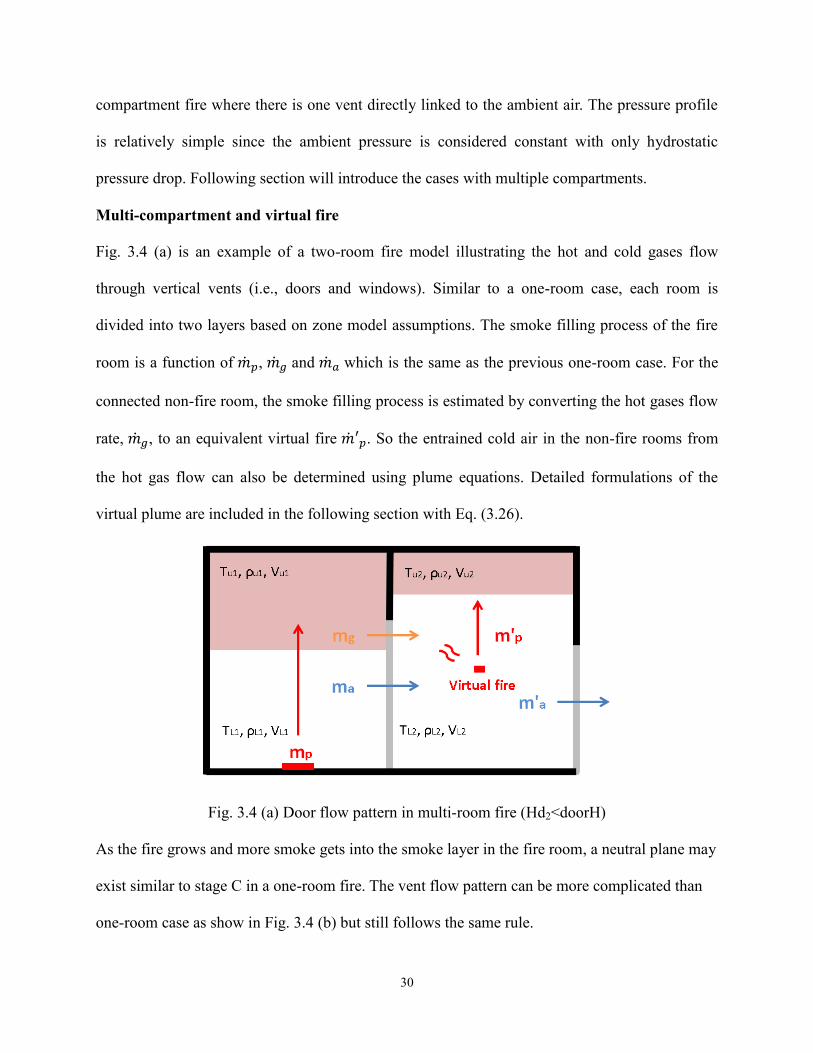
Multi-compartment and virtual fire

Fig. 3.4 (a) is an example of a two-room fire model illustrating the hot and cold gases flow

through vertical vents (i.e., doors and windows). Similar to a one-room case, each room is

divided into two layers based on zone model assumptions. The smoke filling process of the fire

room is a function of ��𝑝, ��𝑔 and ��𝑎 which is the same as the previous one-room case. For the

connected non-fire room, the smoke filling process is estimated by converting the hot gases flow

rate, ��𝑔, to an equivalent virtual fire ��′𝑝. So the entrained cold air in the non-fire rooms from

the hot gas flow can also be determined using plume equations. Detailed formulations of the

virtual plume are included in the following section with Eq. (3.26).

Fig. 3.4 (a) Door flow pattern in multi-room fire (Hd2<doorH)

As the fire grows and more smoke gets into the smoke layer in the fire room, a neutral plane may

exist similar to stage C in a one-room fire. The vent flow pattern can be more complicated than

one-room case as show in Fig. 3.4 (b) but still follows the same rule.

31

Fig. 3.4 (b) Door flow pattern in multi-room fire (Hd2>doorH)

In order to determine the flow rate at door and estimate the model states of each room, it is

formulated as following:

The pressure of a zone is determined by ideal gas law

P = ρ𝑖𝑅𝑇𝑖 (3.1)

where the background pressure of the upper layer and lower layer in the same compartment are

assumed to be identical. And ρ is density of zone air, R is gas constant and T is zone air

temperature. Subscription i represents the location of the layer.

Density

ρ𝑖 =𝑚𝑖

𝑉𝑖 (3.2)

Internal energy

E𝑖 = 𝐶𝑣𝑚𝑖𝑇𝑖 (3.3)

where the mass change over time of the upper layer, ��𝑈, is the sum of the total mass flow

through the upper layer boundary which can be expressed as

d𝑚𝑈

𝑑𝑡= ��𝑈 = ��𝑝 + ��𝑔 (3.4)

32

Since the control volume of each room is constant

V = 𝑉𝑈 + 𝑉𝐿 (3.5)

Next step is to apply energy conservation to a layer which is based on the thermodynamic first

law.

𝑑𝐸𝑖

𝑑𝑡+ 𝑃

𝑑𝑉𝑖

𝑑𝑡= ��𝑖 (3.6)

where ��𝑖 is the rate of total energy gain of a layer including the rate of heat gain and enthalpy

gain through the boundaries.

��𝑈 = ��𝑐 + 𝐶𝑝��𝑝𝑇𝐿 + ��𝑔 𝑟𝑎𝑑 − ��𝑐𝑈 (3.7)

and

��𝐿 = −𝐶𝑝��𝑝𝑇𝐿 − 𝐶𝑝��𝑎𝑇𝐿 + ��𝑐𝐿 (3.8)

Summing up Eq. (3.6) for upper and lower layer

(𝑑𝐸𝑈

𝑑𝑡+

𝑑𝐸𝐿

𝑑𝑡) + 𝑃(

𝑑𝑉𝑈

𝑑𝑡+

𝑑𝑉𝐿

𝑑𝑡) = ��𝑈 + ��𝐿 (3.9)

where

𝑑𝐸𝑈

𝑑𝑡+

𝑑𝐸𝐿

𝑑𝑡=

𝑑(𝑐𝑣𝑚𝑈𝑇𝑈)

𝑑𝑡+

𝑑(𝑐𝑣𝑚𝐿𝑇𝐿)

𝑑𝑡=

𝑐𝑣

𝑅[𝑑(𝑃𝑉𝑈)

𝑑𝑡+

𝑑(𝑃𝑉𝐿)

𝑑𝑡] (3.10)

From Eq. (3.5), the total volume of upper and lower layer is constant so

𝑑𝑉𝑈

𝑑𝑡+

𝑑𝑉𝐿

𝑑𝑡= 0 (3.11)

by substituting Eq. (3.10) and (3.11) into Eq. (3.9).

Then, the differential equation for pressure is obtained

𝑑𝑃

𝑑𝑡=

𝛾 − 1

𝑉(��𝑈 + ��𝐿) (3.12)

At this point, it can be observed that the pressure change over time is a function of total energy

flux entering and leaving the compartment where the mass flow rate from lower layer to upper

33

layer is irrelevant.

Differential equation for upper layer volume

𝑑𝑉𝑈

𝑑𝑡=

1

𝑃𝛾[(𝛾 − 1)��𝑈 − 𝑉𝑈

𝑑𝑃

𝑑𝑡] (3.13)

where the room pressure P is the sum of ambient pressure Pamb and the pressure perturbation ΔP.

P = 𝑃𝑎𝑚𝑏 + ∆𝑃 = 𝑃𝑎𝑚𝑏 +𝑑𝑃

𝑑𝑡∆𝑡 (3.14)

and the rate of temperature and density change for the upper zone can be determined by

𝑑𝑇𝑈

𝑑𝑡=

1

𝑐𝑝𝜌𝑈𝑉𝑈[(��𝑈 − 𝑐𝑝��𝑈𝑇𝑈) + 𝑉𝑈

𝑑𝑃

𝑑𝑡] (3.15)

and

𝑑𝜌𝑈

𝑑𝑡= −

1

𝑐𝑝𝑇𝑈𝑉𝑈[(��𝑈 − 𝑐𝑝��𝑈𝑇𝑈) −

𝑉𝑈

𝛾 − 1

𝑑𝑃

𝑑𝑡] (3.16)

Sub-models

The Heskestad Plume

In order to determine the plume mass flow rate, ��𝑝, in Eq. (3.7) and (3.8), this model applies

empirical correlations proposed by Heskestad (1984) which are a function of fire area, heat

release rate, convective ratio and smoke travel distance. Comparing to other plume models, the

Heskestad plume takes into account fire area and also assumes the fire as a virtual point source

which makes it easier to calculate radiant heat transfer. As illustrated by Fig. 3.5, instead of

directly using the fire area to calculate plume flow rate, Heskestad introduces a virtual origin

point which can convert the plume to a cone shape as an ideal plume. The distance between

actual fire source and the virtual origin, 𝑧0, can be determined by

34

𝑧0 = 0.083��2/5 − 1.02𝐷 (3.17)

where �� is the total heat release rate of the fire source (kW) and D is the diameter of the fire area

(m).

Fig. 3.5 Heskestad’s plume model

Then, the average flame height is given by

L = 0.235𝑄2/5 − 1.02𝐷 (3.18)

And the plume mass flow rate at height z can be expressed as

��𝑝 = 0.071��𝑐1/3

(𝑧 − 𝑧0)5/3 + 1.92 ∙ 10−3��𝑐 𝑓𝑜𝑟 𝑧 > 𝐿 (3.19)

and

��𝑝 = 0.0056��𝑐

𝑧

𝐿 𝑓𝑜𝑟 𝑧 < 𝐿 (3.20)

where ��𝑐 is the convective proportion of the total heat release rate �� and it usually ranges

between 60% to 80% for most fire models.

Orifice equation for vent flow rate

Another set of important variables in the differential equations are the flow rate through the vents

35

denoted ��𝑔 and ��𝑎, which are used to calculate the total energy flux through the boundary of a

layer in Eq (3.7) and Eq (3.8). To obtain the flow rate, the orifice equation is applied where the

velocity at a given height 𝑧 at the opening can be presented as

v(z) = 𝐶𝑑√2∆𝑃(𝑧)

𝜌 (3.21)

where 𝐶𝑑 is the flow coefficient and the mass flow rate is determined by

m = 𝜌𝑣𝐴 = 𝜌𝑣𝑤𝑧 (3.22)

where 𝑤 is the width of the opening.

By substituting velocity 𝑣 with Eq (3.21) and then integrate the equation along the height from

bottom to top of an opening, Eq (3.22) becomes

��𝑣𝑒𝑛𝑡 = ∫ 𝜌𝑣(𝑧)𝑤𝑑𝑧𝑡

𝑏

(3.23)

For a linear pressure profile over a given vertical distance, the equation can be rewritten as

��𝑣𝑒𝑛𝑡 = ∫ 𝐶𝑑√2∆𝑃(𝑧)𝜌𝑤𝑑𝑧 =2

3𝐶𝑑𝐴𝑣𝑒𝑛𝑡√2𝜌 (

𝑃𝑡 + √𝑃𝑡𝑃𝑏 + 𝑃𝑏

√𝑃𝑡 + √𝑃𝑏

)𝑡

𝑏

(3.24)

where 𝑃𝑡 and 𝑃𝑏 are the absolute pressure differences at the top and bottom of the opening

respectively. But the pressure profile over an opening usually has more than one interception

point, as shown in Fig. 3.4, where the calculations of the flow rates need to be divided into

multiple sections.

Equivalent fire plume for non-fire room

The previous section mentioned the smoke filling process of a non-fire room is based on an

equivalent fire plume where the heat release rate is determined by the hot gases flow from the

fire room and can be given by

36

��𝑒𝑞 = 𝑐𝑝(𝑇𝑢1 − 𝑇𝑢2)��𝑔 (3.25)

and the height of the equivalent virtual plume can be expressed as

𝑧𝑝,𝑒𝑞 =(𝐻𝑑1 − 𝐻𝑑2)

��𝑒𝑞2/5

+ 𝑣𝑝 (3.26)

where Hd1 and Hd2 are the smoke layer height of room one and room two respectively and the

virtual point source, 𝑣𝑝, can be determined by the following equations:

𝑣𝑝 = (8.1��𝑝

��𝑒𝑞

)

0.528

for 0 < (𝑚𝑝

��𝑒𝑞

) < 0.0061 (3.27)

𝑣𝑝 = (38.5��𝑝

��𝑒𝑞

)

1.1001

for 0.0061 < (𝑚𝑝

��𝑒𝑞

) < 0.026 (3.28)

𝑣𝑝 = (90.9��𝑝

��𝑒𝑞

)

1.76

for 0.026 < (𝑚𝑝

��𝑒𝑞

) (3.29)

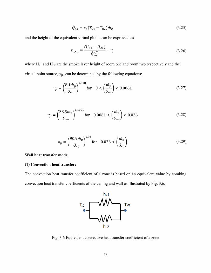
Wall heat transfer mode

(1) Convection heat transfer:

The convection heat transfer coefficient of a zone is based on an equivalent value by combing

convection heat transfer coefficients of the ceiling and wall as illustrated by Fig. 3.6.

Fig. 3.6 Equivalent convective heat transfer coefficient of a zone

37

Based on the ratio of the area, the convective heat transfer coefficient can be determined

h𝑐 =𝐴𝑐𝑒𝑖𝑙𝑖𝑛𝑔

𝐴𝑡𝑜𝑡𝑎𝑙ℎ𝑐,𝑐 +

𝐴𝑤𝑎𝑙𝑙

𝐴𝑡𝑜𝑡𝑎𝑙ℎ𝑐,𝑤 (3.30)

To calculate the heat transfer between the gas layer and the compartment surfaces including

ceiling, walls and floor, three different types of heat transfer models need to be taken into

account: convection, radiation and conduction. Fig. 3.7 shows an example of the heat transfer

occurring at the wall surface where T𝑔 is gas temperature, T𝑤𝑢 is wall temperature and T𝑜𝑢𝑡 is

exterior surface temperature.

Fig. 3.7 Heat balance at wall surface

(2) Radiation heat transfer

Radiation heat accounts for 20% to 40% of the total fire source heat release rate. So the radiation

model is also an important factor to the model accuracy especially for the fire room. In this

model, the fire is assumed to be a point source located in the center of the total flame height

which is L/2 where L can be obtained from Eq. (3.18). First consider the proportion of radiation

heat entering the upper layer, ��𝑡𝑜𝑡𝑎𝑙,𝑟𝑎𝑑.

��𝑡𝑜𝑡𝑎𝑙,𝑟𝑎𝑑 = 𝐹𝑂𝐴𝜀𝜎(𝑇𝑔4 − 𝑇𝑤𝑢

4)A (3.31)

where 𝐹𝑂𝐴 is the view factor of the point fire source to the destination compartment surface, 𝜀 is

the emissivity of the surface material and 𝜎 is the Stefan-Boltzmann constant. 𝑇𝑔 and 𝑇𝑤𝑢 are the

temperature of upper layer gases and wall surfaces respectively. A is the cross section area at the

smoke layer height which is usually the same as ceiling area.

38

To calculate view factor 𝐹𝑂𝐴 for relatively more complicated geometries than a rectangular plane,

the surface can be divided into multiple smaller rectangles and the view factor is approximated

by the sum of all small proportions similar to the example shown in Fig. 3.8.

Fig. 3.8 View factor of a point to a rectangular surface

Consider a point O and a rectangular surface A, the view factor can be

F𝑂𝐴 = 𝐹𝑂1 + 𝐹𝑂2 + 𝐹𝑂3 + 𝐹𝑂4 (3.32)

By applying following equation, the view factor for each segment can be determined

F𝑂1 =1

4𝜋sin−1[

1

√(𝑋2 + 1)(𝑌2 + 1)] (3.33)

where X = z/x and Y = z/y

The same method can also be applied to compute wall and floor view factors while the

orientations of the surface should also be considered to get correct X and Y.

Before the radiation heat flux reaching the wall surface, a certain percentage of the radiation heat

is absorbed by the upper layer gases, denoted ��𝑔,𝑟𝑎𝑑, which is a part of total heat flux, ��𝑈, in Eq

(3.7) and can be expressed as

��𝑔,𝑟𝑎𝑑 = ��𝑡𝑜𝑡𝑎𝑙,𝑟𝑎𝑑 ∙ 𝛼𝑔𝑎𝑠 (3.34)

where 𝛼𝑔𝑎𝑠 is the absorptance of the upper layer gases.

In order to reduce the computation time, the compartment surfaces are assumed to be blackbody

39

where the reflectance is assumed zero.

(3) Transient heat conduction through walls

After obtaining the convection and radiation heat flux at the compartment surfaces, the heat

conduction can also be computed by applying energy balance at the compartment surface as

shown by Fig 3.7. For the material with small heat capacity, the thermal storage within the wall

section can be neglected since it can be considered as thermal penetrated in early stage of fire. So

the calculation can be very easy since the temperature inside the wall is assumed uniform. But

for a thick wall where the temperature gradient inside the wall is significant, one must applies a

transient heat conduction model by dividing the wall into small control volumes using Fourier’s

Law.

(4) Wall surface

The compartment surface temperature is determined by steady state one-dimensional heat

transfer. But for the surfaces with high heat capacity, it is determined by transient heat transfer by

dividing the entire wall section into n control volumes. So the temperature for each control

volume is updated for each time step. For updating the surface temperature 𝑇𝑤 from previous

time I, it can be expressed by

𝑇𝑤𝑖+1 = (1 − 2𝜏 − 2𝜏

ℎ∆𝐿

𝑘) 𝑇𝑤

𝑖 + 2𝜏𝑇1𝑖 + 2𝜏

ℎ∆𝐿

𝑘𝑇𝑎𝑚𝑏 + 𝜏

��𝑤−𝑖∆𝐿

𝑘 (3.35)

where

τ =𝛼𝑤∆𝑡

∆𝐿2 (3.36)

And 𝐿 is the thickness of the wall (m), ∆𝐿 =L/n, k is thermal conductivity of the material

(W/mK), ��𝑤 is the total heat flux to the wall surface including convective and radiant heat

transfer and 𝛼𝑤 is the thermal diffusivity (m2/s)

40

After surface temperature is obtained, the temperature of each control volume inside the wall can

be calculated by

𝑇𝑗−1𝑖 − 2𝑇𝑗+1

𝑖 + 𝑇𝑗+1𝑖 +

��𝑗−𝑖∆𝐿2

𝑘=

(𝑇𝑗𝑖+1 − 𝑇𝑗

𝑖)

𝜏 (3.36)

where j is the index of the control volume and 𝑇0 is the wall surface temperature 𝑇𝑤.

Solving smoke transport problem

The zone model presented in this thesis is based on an explicit method where the model states at

a later time are calculated from the model states at the current time. As shown in Fig. 3.9, the

model is initialized using ambient conditions except the upper layer require a small initial

volume to avoid division-by-zero error. At t = 0, the air flow rate through the door is assumed

zero. The pressure increment is first calculated by energy balance equation and used as initial

value at t = 1. When the pressure is updated, the mass flow at the door can be obtained so the

gradients of volume, temperature and density can be determined. At t = 2, when the temperature

of the upper layer start increasing, the temperatures at the compartment surfaces start updating.

The model is programmed using Java 1.7 and the detailed source codes are presented in

Appendix.

41

Fig. 3.9 Flowchart of zone model numerical operations

3.1.2 Ensemble Kalman filter (EnKF)

The previous chapter briefly introduced the background information about the EnKF. This

chapter introduces the formulation of the EnKF in detail. In general, the numerical operations of

the EnKF can be divided into two steps as shown in Fig. 3.1:

(1) Forecasting step: It is assumed at time step k, there are q numbers of parallel ensemble

42

members for the estimation of the model states, 𝑥𝑘𝑓

, by using normally-distributed sampling

errors. Consider a discrete nonlinear stochastic model

𝑥𝑘𝑓

= f(𝑥𝑘−1, Φ𝑘−1) + 𝑤𝑘−1 (3.37)

where Φ𝑘−1 is the control vector and 𝑤𝑘−1 is a zero mean random white noise at time step k-1.

The measurements corresponding to the model state can be expressed as

𝑦𝑘 = 𝐇𝑥𝑘 + 𝑣𝑘 (3.38)

where the matrix H relates the model state x to the measurement y and v is the observation noise.

If x and y are presenting the same quantity, H can be an identity matrix I.

Assume at time step k, there are q numbers of ensembles that predict models states.

𝐗𝑘𝑓

= [𝑥𝑘𝑓1

, 𝑥𝑘𝑓2

… , 𝑥𝑘𝑓𝑞

] (3.39)

(2) Analysis step: The error covariance, or the expected error of the predicted model states at

analysis points and observation points, can be determined by the ensemble members from Eq.

(3.39).

𝐏𝑘𝑓

𝐇𝑇 =1

𝑞∑(𝑥𝑘

𝑓𝑖− 𝑥𝑘

𝑡 )(𝐇𝑥𝑘𝑓𝑖

− 𝐇𝑥𝑘𝑡 )𝑇

𝑞

𝑖=1

(3.40)

while true state, xkt, is unknown, we use the mean of the ensemble members to approximate the

true state.

𝑥𝑘𝑡 ≈ 𝑥𝑘

𝑓=

1

𝑞∑ 𝑥𝑘

𝑓𝑖

𝑞

𝑖=1

(3.41)

then Eq. (3.40) becomes

𝐏𝑘𝑓

𝐻𝑇 =1

𝑞 − 1∑(𝑥𝑘

𝑓𝑖− 𝑥𝑘

𝑓)(𝐇𝑥𝑘

𝑓𝑖− 𝐇𝑥𝑘

𝑓)𝑇

𝑞

𝑖=1

(3.42)

Please note that in order to make the estimation unbiased, a factor of 1/(q-1) is applied instead of

43

1/q. Then, the Kalman gain can be determined by using the traditional Kalman Filter equation

where an optimum value, xka can also be determined.

PkHT in Eq. (3.42) can be directly obtained from ensemble members and the HPkH

T is a global

matrix for all model states to calculate the covariance between forecast values at the observation

points. It can be noted that for all the q ensemble members, the Kalman gain, K, is always the

same value for all mirrored model states instead of an individual value for each ensemble

member, which significantly reduces the computation cost. In addition, the error covariance

matrix does not need to be saved for the next analysis cycle, which also improves the model

efficiency by releasing memory space for later use.

Fig. 3.10 Flowchart of EnKF forecasting and analysis steps

After Kalman gain is obtained for this time step, analysis can be done to update all model states

even for the model states without direct measurements. For the simulation time step without any

observation available, the prediction of model states is based on the average of all predicted

ensemble members. Meanwhile, one of the common limitations of initial EnKF applications is

44

that in each analysis cycle, the Kalman gain is applied to all model nodes even for those less

correlated so spurious correlations are caused as proven by Evensen (2009). For higher

dimensional models (models with higher number of parameters), it is usually suggested to apply

a distant-dependent Schur-product when using Kalman Gain to update model states (Hamill and

Whitaker, 2001). Detailed discussions about formulating an EnKF model to forecast indoor

environment is presented in Chapter 7.

References

Evensen, Geir. "Sequential data assimilation with a nonlinear quasi‐geostrophic model using

Monte Carlo methods to forecast error statistics." Journal of Geophysical Research: Oceans

(1978–2012) 99, no. C5 (1994): 10143-10162.

Fowkes, N. D. "A mechanistic model of the 1973 and 1974 bedroom test fires." A study of room

fire development: The second full-scale bedroom fire test of the home fire project (July 24,

1974) 2 (1975): 8-50.

Tanaka, Takeyoshi. "A model of multiroom fire spread." Fire Science and Technology 3, no. 2

(1983): 105-121.

Heskestad, Gunnar. "Engineering relations for fire plumes." Fire Safety Journal7, no. 1 (1984):

25-32.

McCaffrey, B. “. "Momentum implications for buoyant diffusion flames."Combustion and

Flame 52 (1983): 149-167.

Zukoski, E. E. "Mass flux in fire plumes." In Fire Safety Science-Proceedings of the Fourth

International Symposium, IAFSS, p. 13. 1994.

Hamill, Thomas M., Jeffrey S. Whitaker, and Chris Snyder. "Distance-dependent filtering of

background error covariance estimates in an ensemble Kalman filter." Monthly Weather

Review 129, no. 11 (2001): 2776-2790.

Evensen, Geir. "The ensemble Kalman filter for combined state and parameter

estimation." Control Systems, IEEE 29, no. 3 (2009): 83-104.

45

Chapter 4 Forecasting Simulations of Indoor Environment using

Data Assimilation via an Ensemble Kalman Filter1

ABSTRACT

Data assimilation is widely used in weather forecasting and other complex forecasting problems

such as hydrology, meteorology, and fire dynamics. Among various data assimilation methods,

the Ensemble Kalman Filter (EnKF) is one of the best solutions to large-scale nonlinear

problems as the computational cost is relatively less intense than other forecasting methods. In

this chapter, a new application of EnKF to forecast indoor contaminant concentrations is

presented. The first part of the paper introduces the fundamental theories of data assimilation.

The second part is a case study of forecasting the concentrations of a tracer gas in a multi-zone

manufactured house by using a mass balance model with an EnKF. The benefits of EnKF and

several important parameters for EnKF were discussed including numbers of ensemble members

and observations, time step of observations, and forecasting lead time. The EnKF method

presented is one of the first studies applied to the indoor environment field. It was shown that by

using EnKF, the predictability of the simple indoor air model for the multi-zone space was

improved significantly.

Highlights:

▪ The EnKF is applied to forecast indoor environment.

▪ The optimum number of ensemble members is approximately 70 to 80.

▪ Both number of observations and time step of observations affect the EnKF performance.

▪ Predictability of the indoor model is significantly improved with EnKF implementation.

1. The contents of this chapter are published in (Lin, Cheng-Chun, and Liangzhu Leon Wang“. "Forecasting

simulations of indoor environment using data assimilation via an Ensemble Kalman Filter." Building and

Environment 64 (2013): 169-176. The contents are slightly updated.

46

4.1 Introduction

4.1.1 Forecasting contaminant transport

The forecasting of indoor environment is of great interests due to its close relationship to

occupant’s safety (Koo et al. 2010), thermal comfort (Freire et al. 2008), and energy efficiency

(Oldewurtel et al. 2012 and Tudoroiu et al. 2008), for which an accurate prediction of important

parameters is often needed such as temperature, relative humidity and contaminant

concentration. Forecasting these indoor air properties, especially solving contaminant transport

problem in a dynamic environment, is a difficult task since the physical states of the building

environment could change rapidly over time (Liu and Zhai 2009). Under such uncontrollable

factors as ambient temperature, air velocity, humidity, and occupant loads, the contaminant

estimation is hard to achieve by conventional methods using steady state analysis of constant

model parameters. In addition, sudden release of contaminant, opening doors and windows,

change of occupant behavior and the use of electric appliances are a few common examples that

may further increase the difficulty of solving the forecasting problem. By using any numerical

model to predict future indoor air contaminants, these uncertain events will cause the predicted

physical states to depart from reality as the model evolves forward over time. Previous studies

showed a few different ways of indoor environment forecasting. Federspiel (1997) utilized a

method originating from the optimization theory, so-called the Kalman Filter, to estimate the

strength of gas sources in buildings successfully. But the model has some restrictions when it

applies to multi-zone problems since source strength and air flow rate must be known a priori.

Kemajou (2012) presented that indoor air temperature and relative humidity could be quickly

predicted by using artificial neural network (ANN). The potential problem of using a black-box

type of methods like ANN is that the training of models still relies on trial and error to determine

47

an optimum model structure while the training parameters usually cannot be applied to other

buildings. Another limitation is its inefficiency for each new case, in which huge amount of data

is required for the training. Sreedharan (2006) introduced another model of forecasting

simulation using Bayesian Monte Carlo method to quickly analyze measurements from multiple

indoor air sensors. This system can monitor real-time indoor environment to help protect

occupants by locating the release source of a high-risk pollutant. Follow-up studies (Gadgil et al.

2008 and Sreedharan 2011) focus more on using heterogeneous sensor systems such as

monitoring door position and mechanic ventilation operating status. Extensive reviews of other

methods for locating indoor air contaminants can be found in the article conducted by Liu and

Zhai (2007). Most of these previous studies focus on locating contaminant source instead of

predicting dynamic future evolvement of concentrations in a multi-zone building.

4.1.2 Data assimilation

The major task of forecasting simulations is to predict future states of physical phenomenon with

a certain lead time and accuracy. In order to find optimal state variables, data assimilation

provides different algorithms for parameter estimation while taking into account uncertainties of

measurements and numerical predictions.

In 1960, a pioneer research of data assimilation theory has been established by R. E. Kalman, the

Kalman Filter, which provides a recursive solution to find a best possible estimation of the true

state. Instead of finding an optimal estimation for one value as best linear unbiased estimation

(BLUE), the Kalman Filter can be applied to a dynamic model that evolves over time (Welch and

Bishop 2006 and van Velzen 2010). In order to solve different types of nonlinear problems, a few

Kalman Filter variants have been proposed. In the Extended Kalman Filter (XKF), the nonlinear

models are linearized by using partial derivatives which is similar to a Taylor series expansion. It

48

has been proven that XKF is effective in many applications but its weakness is the error

probability density is not fully considered in the linearization. Although the analysis scheme of

XKF is similar to traditional Kalman Filter, the computational requirements of XKF are

drastically increased by additional numerical operations, such as linearization. Another

mainstream of the data assimilation theories for nonlinear problems is four-dimensional

variational assimilation (4D-Var) and is widely used to weather forecasting (Courtier 2007). Like

its counterpart, three-dimensional variational assimilation (3D-Var), 4D-Var is based on

minimizing a cost function. In order to calculate the gradient of the cost function for

minimization, it is required to manipulate large matrices, which makes 4D-Var computationally

intensive. Evensen (1994) proposed a more affordable method, Ensemble Kalman Filter, to

determine error statistics by using the Monte Carlo method. The method reduces computational

requirement of XKF by using ensemble members, which are similar to the samplings in other

Monte Carlo methods, to avoid direct calculation and storage of the evolution of the large error

covariance matrices. Each ensemble member in EnKF can be calculated separately so it is

especially suitable for parallel computing and solving large scale problems. This method has

been widely used in weather forecasting, hydrology and fire dynamics predictions (van Velzen

2010 and Jahn 2010). No previous studies have been reported to use EnKF for indoor

environment simulations. Different from existent studies, the indoor air forecasting model with

the EnKF is performed without determining source strength and location but instead depending

on the accurate estimation of error statistics including uncertainties from both experiment and

numerical model. Therefore the EnKF can perform faster prediction than other methods but

relies on rapidly obtaining measurement data.

The objective of this paper is to explore the applications of EnKF to forecasting indoor air

49

environment and discuss the key parameters involved in the accuracy of EnKF for indoor

environment forecasting. This paper applied an EnKF to a case study of forecasting the

concentrations of a tracer gas in a multi-zone manufactured house by using a mass balance

model. The benefits of EnKF and several important parameters for EnKF were discussed

including numbers of ensemble members and observations, time step of observations, and

forecasting lead time. The EnKF method presented is one of the first studies applying a weather

forecasting model to indoor environment field. In this paper, all numerical operations relating to

data assimilation are based on a generic toolbox for data assimilation, OpenDA (Verlaan et al.

2010), developed by Delft University of Technology, Netherland.

4.2 Methodology

The detailed explanations on data assimilation and the fundamental theories of EnKF can be

found in many references (Kálmán 1960, Welch et al. 2006, Evensen 1994 and Verlaan et al.

2010) so they are not covered in this paper to avoid repetition. Instead of copying down the math

of EnKF, this paper will focus on how the fundamental methodology of EnKF is applied to the

indoor air modeling of a multi-zone manufactured house.

4.2.1 Multi-zone manufactured house

The experimental data for data assimilation come from a series of tracer gas measurements in a

manufactured house conducted by National Institute of Standards and Technology (NIST) in

2007 (Nabinger and Persily 2008, Wang and Emmerich 2010). The house includes living room,

family room, kitchen and three bedrooms as shown in Fig. 4.1. An attached garage was added

after the measured data were collected so it was not included in this study. During the

experiment, tracer gas, sulfur hexafluoride (SF6), was injected about every six hours in the living

room and the concentration of SF6 was measured at various indoor locations for every ten

50

minutes by gas chromatography. The system is capable of measuring SF6 concentration over a

range of 3 to 300 ppb, with an uncertainty of about 5 % of the reading. In this study, bedroom 3

was excluded because its sampling line was moved to the outside for another research project.

Please note that the measurement of each room starts from different time step as shown in Table

1.1. For example, the tracer gas concentration in the master bedroom was measured at t = 0, 10

min and so on, and bedroom 2 is measured at t = 1, 11 min etc. The average air change between

indoors and outdoors was calculated based on the tracer gas decay method, which was about 0.1

to 0.4 air changes per hour (ACH). In this study, twelve hours measurement data are obtained

from four different locations as observation while two injections are included. The first one is at

the beginning of the experiment and the other one is about six hours after the first injection. The

injection rate is intended to achieve an average initial gas concentration of around 120 ppb but is

assumed to be unknown in the simulations. The instruments were calibrated regularly and

believed to be accurate enough. 5% error is thus assigned to the observation errors accounting for

the mentioned uncertainties. The uncertainties associated with the mixing conditions are

considered in the numerical model in the following sections.

Fig. 4.1 CONTAM model of the manufacture house (Wang and Emmerich 2010).

51

Table 4.1 Summary description of the manufactured house and the tracer measurement. Room Master Bedroom Bedroom 2 Living Room Family Room Kitchen

Volume (m3) 35 28 80 50 40

Initial Concentration (ppb) 103 160 145 143 142

First Observation (min) 0 1 4 5 7

4.2.2 Tracer gas concentration model

The modeling of indoor environment here is to forecast the SF6 concentrations in the different

rooms of the house by a mass balance model of SF6. The forecasting accuracy of the model is

improved by combining with measured SF6 concentrations following the algorithm of the EnKF.

Based on the well-mixed assumption, which assumes the air property within a room/zone is well

mixed without spatial variation, the mass balance for a contaminant in one room can be

determined by

𝑑𝐶

𝑑𝑡(𝜌𝑖𝑛𝑉) = 𝑆𝑐 − ∑ 𝜌𝑖𝑛𝐶𝑄𝑜𝑢𝑡𝑓𝑙𝑜𝑤 + ∑ 𝜌𝑜𝑢𝑡𝐶𝑜𝑢𝑡𝑄𝑖𝑛𝑓𝑙𝑜𝑤 (4.1)

where V is the volume of the room, Sc is the contaminant source generation rate, ρ is the density

of the room air and Q is the air volumetric flow rate. Subscripts in and out indicate the flow

direction relative to each room. The contaminant concentration for each room at time k, C𝑘, can

be discretized in time as

𝐶𝑘 = 𝐶𝑘−1 +

𝑑𝐶𝑘−1

𝑑𝑡∆t (4.2)

where 𝑑𝐶𝑘−1

𝑑𝑡 is evaluated by Eq. (4.1) and can be solved numerically by a method such as the

Runge-Kutta method.

Eqs. (4.1) and (4.2) are applied to five zones including family room, master bedroom, kitchen,

living room and bedroom 2. The airflow rates among the different rooms, Q, are calculated by

using the multi-zone indoor air quality analysis software, CONTAM (Walton and Dols 2010),

with hourly averaged weather conditions as inputs. The weather conditions were measured by a

52

local weather station at the house site. The detailed simulation results are shown in the results

and discussions section.

4.2.3 Stochastic model of tracer gas concentration

Eq. (4.1) is a conventional deterministic model when the model parameters, either obtained

numerically or experimentally, are without considering uncertainties. For complex problems

and/or systems with high uncertainties, the analysis is commonly based on stochastic models to

reflect the randomness or the probability distribution of the model variables. Therefore, Eq. (4.1)

needs to be converted into a stochastic model by perturbing the model variables with an auto-

regression model during the Monte Carlo sampling process of the EnkF (Thornber 1967). An

example of setting up the uncertainties is that the calculated airflow rates in CONTAM are

expected to have 10 % deviations from the hourly variations of the experiment day. The error

from CONTAM simulation and the well-mixed assumption accounts for another 10 % deviation.

The selection of these uncertainties should be evaluated under different conditions but currently

is not the focus of this paper. Here we define these deviations as zero-mean, normally-distributed

white noise. Based on the probability density of these deviations, the model parameters for each

Monte Carlo sample, here so-called an ensemble member, are generated.

4.2.4 Combining numerical prediction and measurements by EnKF

By using the EnKF, the stochastic model is combined or so-called assimilated with the

measurements in different rooms. In this study, the measurements from four rooms are used at

current time step: the master bedroom, family room, kitchen and bedroom 2, in the data

assimilation to forecast the concentrations in all rooms in the future, especially that of the living

room, where no experimental data have been used. A data assimilation forecasting of a

contaminant concentration at the time k for a room j, 𝐶𝑗,𝑘𝑓

, can be expressed by:

53

𝐶𝑗,𝑘𝑓

= f(𝐶𝑗,𝑘−1, Φ𝑗,𝑘−1) + 𝑤𝑗,𝑘−1 (4.3)

where f means forecasting, j is the index of model nodes and k is the index of time; Φ𝑗,𝑘−1 is the

control vector which represents perturbed airflow rates and 𝑤𝑗,𝑘−1 is a zero mean random white

noise accounts for simulation errors at time step k-1. The function f here refers to Eq. (4.2).

When any observation is available, the true state of the living room concentration, 𝐶𝐿,𝑘𝑡 , is

estimated by EnKF. For example, at t = k min, the measurement is available in the master

bedroom so the EnKF is able to work as follows. A vector of the predicted SF6 concentration is

generated by the ensemble members with a total number of q for each room, e.g. the

concentration forecast of the master bedroom can be presented as

𝐶𝑀𝐵,𝑘𝑓

= [𝐶𝑀𝐵,𝑘𝑓1

, 𝐶𝑀𝐵.𝑘𝑓2

… , 𝐶𝑀𝐵,𝑘𝑓𝑞

] (4.4)

The measurement in the master bedroom corresponding to the numerical forecast is expressed as

𝑦𝑀𝐵,𝑘 = 𝐇𝐶𝑀𝐵,𝑘𝑓

+ 𝑣𝑘 (4.5)

where the matrix H relates the model state 𝐶𝑀𝐵,𝑘𝑓

to the measurement 𝑦𝑀𝐵,𝑘 and 𝑣𝑘 is the

observation noise (accounts for 5 % measurement error in this case). If 𝐶𝑀𝐵,𝑘 and 𝑦𝑀𝐵,𝑘 represent

the same physical quantity, H will be the identity matrix, I.

Then the forecast error covariance, or expected error of the model prediction, 𝑃𝑀𝐵,𝑘𝑓

, can be

approximated by the q ensemble members:

𝐏𝑀𝐵,𝑘𝑓

𝐇𝑇 =1

𝑞∑(𝐶𝑀𝐵,𝑘

𝑓𝑖− 𝐶𝑀𝐵,𝑘

𝑡 )(𝐇𝐶𝑀𝐵,𝑘𝑓𝑖

− 𝐇𝐶𝑀𝐵,𝑘𝑡 )𝑇

𝑞

𝑖=1

(4.6)

since the true state, 𝐶𝑀𝐵,𝑘𝑡 , is unknown, we use the mean of the ensemble members to

approximate

54

𝐶𝑀𝐵,𝑘𝑡 ≈ 𝐶𝑀𝐵,𝑘

𝑓 =

1

𝑞∑ 𝐶𝑀𝐵,𝑘

𝑓𝑖

𝑞

𝑖=1

(4.7)

then Eq. (4.6) becomes

𝐏𝑀𝐵,𝑘𝑓

𝐇𝑇 =1

𝑞 − 1∑(𝐶𝑀𝐵,𝑘

𝑓𝑖− 𝐶𝑀𝐵,𝑘

𝑓 )(𝐇𝐶𝑀𝐵,𝑘

𝑓𝑖− 𝐇𝐶𝑀𝐵,𝑘

𝑓 )𝑇

𝑞

𝑖=1

(4.8)

Please note that in order to make the estimation unbiased, a factor of 1/(q-1) is applied instead of

1/q (Whitaker 2002). Then, the Kalman gain for the master bedroom, KMB,K, can be determined

by using the traditional Kalman Filter equation where an optimal master bedroom

concentration,𝐶𝑀𝐵,𝑘𝑎 , is estimated as

𝐶𝑀𝐵,𝑘𝑎 = 𝐶𝑀𝐵,𝑘

𝑓 + 𝐊𝑀𝐵,𝑘(𝑦𝑀𝐵,𝑘 − 𝐇𝐶𝑀𝐵,𝑘

𝑓 ) (4.9)

where the Kalman gain for each room at t=k, 𝐊𝑗 can be estimated by

𝐊𝑗,𝑘 =

𝐏𝑗,𝑘𝐇𝑇

𝐇𝐏𝑀𝐵,𝑘𝐇𝑇 + 𝐑 (4.10)

where the denominator of Eq. (4.10) is a constant for all Kalman gains since the measurement is

only available in master bedroom and R presents the expected measurement error (5% in this

case). The numerator can be obtained without using any measurement by calculating the

respective error covariance 𝑃𝑗,𝑘𝐻𝑇 for each room. KMB,k = Kj,k when Pj,k is PMB,k. After obtaining

all five Kalman gains, the concentration can be updated for all five rooms even for those without

measurements by Eq. (4.9). So the true state of the living room 𝐶𝐿,𝑘𝑡

can be approximated by 𝐶𝐿,𝑘𝑎

which combines results of numerical prediction and experimental measurements. For the

simulation time step without any observation available, the prediction of model states is based on

the average of all predicted ensemble members. Since the predicted model states are sequentially

assimilated with the measurements, the error covariance matrix does not need to be saved for the

55

upcoming analysis cycle, which reduces the computational cost by releasing memory space for

later use.

4.3 Results and discussions

4.3.1 CONTAM airflow rate simulations

Fig. 4.2 illustrates the transient airflow rates predicted from CONTAM simulations used in the

forecasting simulation of SF6 concentrations. The airflow rate between the indoor and exterior

environment varies over time due to the change of weather condition while the interior airflow

rate are relative constant. Table 4.2 shows the average airflow rate between two neighboring

rooms. It can be observed that interior air exchange is generally much higher than the exterior.

Therefore, the dynamic model (e.g. Eq. 4.2) is calculated with a one-minute time step (Δt = 1

minute) by assuming constant airflow rates for the interior air exchange and time-dependent

airflows for the exterior exchange during the simulation. Like most existent indoor air

forecasting model, the deterministic model use measurement data from the sensors directly as

inputs where the uncertainties are not considered in this case.

Fig. 4.2 Examples of transient airflow rates from CONTAM outputs.

1350

1375

1400

1425

1450

-20

-10

0

10

20

0 120 240 360 480 600 720

Inte

rio

r A

irfl

ow

Rat

e (m

3/h

r)

Exte

rio

r A

irfl

ow

Rat

e (m

3/h

r)

Time (minutes)

Living room to Outdoor

Outdoor to living room

Kitchen to Family Room

56

Table 4.2 Average airflow rates in the house (m3/min).

From

To

Master

Bedroom

Bedroom 2 Living

Room

Family

Room

Kitchen Outdoor

Master Bedroom N/A 9.70 N/A 0.0 0.0

Bedroom Two N/A 7.70 N/A N/A 0.0

Living Room 9.44 7.66 N/A 25.43 0.17

Family Room 0.0 N/A N/A 26.36 0.14

Kitchen 0.01 N/A 24.79 26.59 0.09

Outdoor 0.04 0.02 0.04 0.0 0.0

Fig. 4.3 Comparisons of deterministic sequential simulation and EnKF with the measured SF6 in

the living room.

4.3.2 Tracer gas forecasting with and without EnKF

To demonstrate the benefits of using EnKF, we first directly use the deterministic model of Eq.

(4.2) to predict SF6 concentration in the living room as a control group for comparison. In both

cases, the measurements of all rooms except the living room at the previous time step are given

as the inputs to predict the concentration at the current time by Eq. (4.2), and only the initial

concentration is given in the living room. In Fig. 4.3, the deterministic (non-EnKF) model has

shown good predictability when there is no sudden change in SF6 concentration. But when the

second SF6 injection took place around the 350 minutes, the model will require about 30 minutes

to correct the prediction in the living room as illustrated by the bold horizontal bar in Fig. 4.3,

since there is no direct measurement available. The slow response of the non-EnKF model is due

40

60

80

100

120

140

160

0 120 240 360 480 600 720

Co

nce

ntr

atio

n (

pp

b)

Time (min)

Measurements

EnKF

Non-EnKF

57

to the reason that the measurement at one room is only used to update the model state for that

room but its impact on other rooms is not taken into account since Kalman gain is not calculated.

By implementing EnKF when one measurement is available, Kalman gains can be computed for

all the modeled nodes. Therefore, one measurement can update the concentrations for all nodes

even for those without measurements. The analyzed states are then used in the dynamic model as

a new initial condition to compute new model states in the following time steps. When the next

observation is available, the procedure is then repeated. As shown by the bold line in Fig. 4.3, the

predictability improves significantly with the EnKF implementation near the time of the

injection.

4.3.3 Discussion of key EnKF parameters

In this section, we will discuss how different key parameters affect the accuracy of the EnKF

during the indoor environment modeling in the case study. These parameters include number of

ensemble members, number of observations, observation time step, the effects of weather

conditions, forecasting lead time and finally the predictability.

Number of ensemble members

During the forecasting, the model states are determined by the average of all ensemble members

as shown by Eq. (4.7). Fig. 4.4 illustrates the predicted concentration of the living room from 70

ensemble members in grey lines and the black line is the average of all ensemble members when

compared to the measurements (the black squares). Although a single ensemble member may

vary significantly about the ensemble average, the average is very close to the experimental data,

which indicates 70 ensemble members are appropriate to provide the accurate prediction in this

case. From Eq. (4.8), the error statistics are estimated based on a finite size of ensemble members

to approximate q→∞. For a simple model with low number of mesh grids or data points, q not

58

only affects the predictability but also determines the computational cost of the analysis. Table

4.3 shows that the simulation time increased with the number of ensemble numbers. Considering

both accuracy and cost, 70 ensemble members seem to be the best choice for the modeled house.

In general, it is recommended to have around 100 ensemble members in many EnKF

applications since the results are not showing significant improvement by exceeding this number.

In addition, the computational burden also increases drastically with the ensemble members

(Evensen 2009). Thulin and Nævdal (2011) also suggested doing several EnKF runs in which

each with less ensemble members. We also simulated the same house under different weather

conditions, i.e. November and February in Fig. 4.5, and obtained consistent results. It shows the

optimum numbers of ensemble members for both cases are very close (q = 70 and q = 80).

Unfortunately, there is still no theoretical principles to determine an optimal ensemble number

but it is recommended to start trial and error from q = 100. For all cases, the simulations only

takes a few seconds, which shows the EnKF is very fast for this case.

Fig. 4.4 EnKF prediction of the living room concentration by 70 ensemble members.

0

50

100

150

200

380 400 420 440 460 480 500

Time (minute)

Co

nc

en

tra

tio

n (

pp

b)

59

Table 4.3 Comparisons of root mean squared errors of different models

Case 1 2 3 4 5 6 7

Ensemble numbers 30 50 70 90 110 70 70

Observations nodes 4 4 4 4 4 3 2

CPU time (seconds) 4 7 10 14 18 11 7

RMSE living room SF6 (ppb) 7.1 7.3 5.4 5.3 6.9 7.9 8.8

Fig. 4.5 Comparisons of the RMSE of the November and February cases (CV is the coefficient

of variation. Defined as the RMSE divided by the mean).

Number of observations

The number of observations also plays a role in performance of EnKF. As shown by case 3, 6

and 7 in Table 4.3, the RMSE decreases when more observed nodes available for data

assimilation for q = 70. It is not surprising because more data available for assimilation would

improve the accuracy of the prediction. For a real-time indoor air monitor system, the problem is

the optimal number of sensors and the best location to place in a multi-zone environment to

achieve certain forecasting accuracy. Fig. 4.6 shows that when the observations were only

provided for the kitchen and family room, the prediction in the living room seems still reasonable,

of which the RMSE is 8.8 ppb as shown by case 7 in Table 4.3. More studies using other

combinations of two observation nodes or even one node are beyond the scope of this paper but

are indeed worth further investigations.

0

4

8

12

16

30 40 50 60 70 80 90 100 110 120

Ensemble N umber q

CV

(RM

SE

) (%

)

N ovember

February

60

Fig. 4.6 Comparisons of the SF6 prediction in the living room by different numbers of

observations (“obs = K and F” means observation data are only provided for kitchen and family

room).

To complete this section, Fig. 4.7 shows the posteriori estimations of SF6 concentration in the

master bedroom. Different from the forecasted data in Fig. 4.8, the posteriori estimations in

Fig .4.7 are assimilated with local observation in the master bedroom so the results are very close

to the measurements. The similar results are also found for kitchen, family room and bedroom 2.

Fig. 4.7 Posteriori estimations of the SF6 concentration in master bedroom.

90

100

110

120

130

140

150

0 20 40 60 80 100 120

Co

nce

ntr

atio

n (

pp

b)

Time (minute)

Measurements

obs = K, F, MB and B2

obs = K, F and MB

obs = K and F

100

110

120

130

140

150

0 20 40 60 80 100 120

T ime (minute)

Co

ncen

trati

on

(p

pb

)

M easurement s

EnK F

61

Observation time step

Commercial off-the-shelf (COTS) sensors with desired resolution to analyze indoor air

commonly have 10 to 30 minutes response time (Won and Schleibinger 2011), which is slow for

an EnKF forecast for faster response. One of the remedies would be to arrange all sensors in a

sequential order that successively and continuously acquires observed data from different nodes,

instead of concurrent sampling that collects all sensor measurements simultaneously. With EnKF,

the forecasting can be updated for all modeled nodes even with only one measurement, no matter

which node the measurement comes from. As a result, as far as the EnKF is concerned, the

sensor response time can be shortened when using the sequential sampling.

For the current study, four gas samplings were supplied sequentially to one gas chromatography

(GC) so each room will have a measurement every 10 minutes, equivalent to a sensor response

time of 10 minutes, whereas an observation for the EnKF is available approximately every 2.5

minutes due to the sequential sampling process, if every observation is used for data assimilation.

To study the impact of the sensor response time on the forecast, Fig. 4.8 illustrates a comparison

of the models with different observation time steps. When the sensor response time increases

from 10 minutes to 20 or 30 minutes (observation time step equals to 2.5, 5.0 and 7.5 minutes

respectively), the predicting errors also increase. Although instruments with shorter response

time and higher resolution can increase forecasting accuracy, further studies are necessary to

determine the tradeoffs among sensor resolution, quantities and response time to the system costs,

which is beyond the scope of this paper. However, it is shown that the sensor response time and

the sampling strategy are important for the accuracy of the EnKF.

62

Fig. 4.8 Comparisons of the EnKF predictions models with different observation time steps.

Forecasting lead time and predictability

Another important character of a data assimilation simulation is the forecasting lead time. Fig.

4.9 shows the predictability of the model during the second injection when the observations were

stopped being provided for data assimilation at different time step. For example, the grey line

with squares starts, tstop = 340 min, represents the observations are not provided after t = 340 min.

Since the tracer gas was injected at around t = 350 min, new measurements are required to

update the model states so the model fails to predict the injection. By feeding the new

measurements from t = 350 to 360 min, the posteriori estimation switches to the bold solid line

associated with an improvement of predictability. When the observation feeding then stops at t =

360 min, i.e. the grey line with crosses, the prediction is shown to be within five percent

measurement error range only for about 10 mins after SF6 injection. When more measurements

were provided from t = 360 to t = 370 min, the forecasting improves as shown by the grey line

with solid squares. This illustrates that in times of an unpredicted major change of indoor air

properties, the forecast will require approximate 10 minutes to reach a stabilized model state and

provide 60 minutes lead time in prediction. By comparing to the non-EnKF model illustrated by

100

110

120

130

140

150

0 20 40 60 80 100 120

Co

nce

ntr

atio

n (

pp

b)

Time (minute)

Measurements

obs. time step = 2.5 mins

obs. time step = 5.0 mins

obs. time step = 7.5 mins

63

the bold dotted line, it requires at least 25 minutes to allow posteriori estimation to get into five

percent error range. It can be concluded that by providing four sensors with 10 minutes response

time (average 2.5 minutes observation time step), the model can quickly respond to sudden

concentration changes and provides high quality predictions after about 10 minutes following the

injection. When the data is fed continuously without being stopped until tstop = 440 min, the

model provides the best accuracy as illustrated by the solid line in the figure.

Fig. 4.9 Predictability of the model near the second injection of SF6 (e.g. tstop = 350 means the

observation data feeding for data assimilation stops at t = 350 min).

4.4 Conclusions

This paper applied a new methodology of using an EnKF to forecast the dispersion of

contaminant as simulated by a tracer gas in an indoor environment based on the assimilation of

multiple sensor data with a mass balance stochastic model. A general setup and key parameters

of the model were discussed. By sequentially implementing measurements from different

sensors, data assimilation can be performed more frequently to improve model performance.

Different from other existing research using the Monte-Carlo method, the reported model in this

50

70

90

110

130

150

320 340 360 380 400 420

T im e (m inute)

Co

nc

en

tra

tio

n (

pp

b)

M e a su re m e n ts

tsto p = 3 4 0 m in s

tsto p = 3 5 0 m in s

tsto p = 3 6 0 m in s

tsto p = 3 7 0 m in s

tsto p = 3 8 0 m in s

tsto p = 4 2 0 m in s

N o n -En KF

64

paper avoids estimating source strength and location in order to reduce the sampling numbers

and still provide noticeable predictability. Overall, this paper concludes that the benefits of using

EnKF to forecast indoor air environment are significant. Future research is needed to apply the

EnKF to other simulation problems, e.g. computational fluid dynamics, and confirm the results

to longer time duration, e.g. a few days or weeks, and other practical cases. It is also necessary to

study the tradeoffs among sensor resolution, quantities and response time to the system costs in

the future research.

Acknowledgment

This research is supported by Concordia University New Faculty Startup Funds. The authors

thank Dr. Nils van Velzen for assisting OpenDA programming and the indoor air quality and

ventilation group at the U.S. National Institute of Standards and Technology for providing

experimental data.

References

Koo, Sung-Han, Jeremy Fraser-Mitchell, and Stephen Welch. "Sensor-steered fire

simulation." Fire Safety Journal 45, no. 3 (2010): 193-205.

Freire, Roberto Z., Gustavo HC Oliveira, and Nathan Mendes. "Predictive controllers for thermal

comfort optimization and energy savings." Energy and buildings 40, no. 7 (2008): 1353-1365.

Oldewurtel, Frauke, Alessandra Parisio, Colin N. Jones, Dimitrios Gyalistras, Markus Gwerder,

Vanessa Stauch, Beat Lehmann, and Manfred Morari. "Use of model predictive control and

weather forecasts for energy efficient building climate control." Energy and Buildings 45 (2012):

15-27.

Tudoroiu, Nicolae, Mohamed Zaheeruddin, E-R. Tudoroiu, and Victor Jeflea. "Fault detection

and diagnosis (FDD) in heating ventilation air conditioning systems (HVAC) using an interactive

multiple model augmented unscented Kalman filter (IMMAUKF)." In Human System

Interactions, 2008 Conference on, pp. 334-339. IEEE, 2008.

Liu, Xiang, and Zhiqiang John Zhai. "Prompt tracking of indoor airborne contaminant source

location with probability-based inverse multi-zone modeling." Building and Environment 44, no.

6 (2009): 1135-1143.

65

Federspiel, Clifford C. "Estimating the inputs of gas transport processes in buildings." Control

Systems Technology, IEEE Transactions on 5, no. 5 (1997): 480-489.

Kémajou, Alexis, Léopold Mba, and Pierre Meukam. "Application of Artificial Neural Network

for Predicting the Indoor Air Temperature in Modern Building in Humid Region." British

Journal of Applied Science & Technology 2, no. 1 (2012): 23-34.

Sreedharan, Priya, Michael D. Sohn, Ashok J. Gadgil, and William W. Nazaroff. "Systems

approach to evaluating sensor characteristics for real-time monitoring of high-risk indoor

contaminant releases." Atmospheric Environment 40, no. 19 (2006): 3490-3502.

Gadgil, Ashok, Michael Sohn, and Priya Sreedharan. "Rapid Data Assimilation in the Indoor

Environment: Theory and Examples from Real-Time Interpretation of Indoor Plumes of Airborne

Chemical." In Air Pollution Modeling and Its Application XIX, pp. 263-277. Springer

Netherlands, 2008.

Sreedharan, Priya, Michael D. Sohn, William W. Nazaroff, and Ashok J. Gadgil. "Towards

improved characterization of high-risk releases using heterogeneous indoor sensor

systems." Building and Environment 46, no. 2 (2011): 438-447.

Liu, X., and Z. Zhai. "Inverse modeling methods for indoor airborne pollutant tracking: literature

review and fundamentals." Indoor air 17, no. 6 (2007): 419-438.

Kalman, Rudolph Emil. "A new approach to linear filtering and prediction problems." Journal of

Fluids Engineering 82, no. 1 (1960): 35-45.

Welch, Greg, and Gary Bishop. "An introduction to the Kalman filter." (1995).

Van Velzen, N. "A Generic Software Framework for Data Assimilation and Model

Calibration." Delft University of Technology, Delft (2010).

Talagrand, Olivier, and Philippe Courtier. "Variational assimilation of meteorological

observations with the adjoint vorticity equation. I: Theory. "Quarterly Journal of the Royal

Meteorological Society 113, no. 478 (1987): 1311-1328.

Evensen, Geir. "Sequential data assimilation with a nonlinear quasi‐geostrophic model using

Monte Carlo methods to forecast error statistics." Journal of Geophysical Research: Oceans

(1978–2012) 99, no. C5 (1994): 10143-10162.

Jahn, Wolfram. "Inverse modelling to forecast enclosure fire dynamics." (2010).

Verlaan, M., Velzen Nv, and S. Hummel. "A generic toolbox for data assimilation in numerical

modeling." In 15th biennial conference of the joint numeric. 2010.

Nabinger, S. J., and A. K. Persily. "Airtightness, Ventilation and Energy Consumption in a

Manufactured House: Pre-Retrofit Results." National Institute of Standards and

66

Technology (2008).

Wang, Liangzhu Leon, and Steven J. Emmerich. "Modeling the effects of outdoor gasoline

powered generator use on indoor carbon monoxide exposures." In Building Simulation, vol. 3,

no. 1, pp. 39-50. Tsinghua Press, 2010.

Walton, G. N., and W. S. Dols. "Contam 3.0 user guide and program documentation." National

Institute of Standards and Technology Technical Report NISTIR 7251 (2010).

Thornber, Hodson. "Finite sample Monte Carlo studies: An autoregressive illustration." Journal

of the American Statistical Association 62, no. 319 (1967): 801-818.

Whitaker, Jeffrey S., and Thomas M. Hamill. "Ensemble data assimilation without perturbed

observations." Monthly Weather Review 130, no. 7 (2002): 1913-1924.

Evensen, Geir. "The ensemble Kalman filter for combined state and parameter

estimation." Control Systems, IEEE 29, no. 3 (2009): 83-104.

Nævdal, Geir, Kristian Thulin, Hans Julius Skaug, and Sigurd Ivar Aanonsen. "Quantifying

Monte Carlo uncertainty in the ensemble Kalman filter." SPE Journal 16, no. 01 (2011): 172-

182.

Won, D. Y., and H. Schleibinger. "Commercial IAQ Sensors and their Performance Requirements

for Demand-Controlled Ventilation." (2011).

67

Chapter 5 Forecasting Smoke Transport during Compartment Fires

using a Data Assimilation Model1

Abstract

Forecasting simulation of an unknown compartment fire is challenging and usually accompanied

with large number of uncertainties. As the simulation progress over time, the forecasted physical

conditions such as fire heat release rate, room temperature and vent airflow rate may sway from

the reality in a highly dynamic environment. Conventional deterministic fire simulation tools

using one set of initial inputs to predict fire smoke transport may not easily generate satisfactory

results. In this paper, a new application of Ensemble Kalman Filter (EnKF) to forecast smoke

dispersion during compartment fires is presented. The model utilizes measurement data from

multiple sensors in multi-room compartments and is able to predict fire heat release rate and

smoke dispersions within several minutes. In addition, detailed formulation of the EnKF model

and three case studies are also discussed in the paper. The resulting model can be considered as a

prototype forecast simulation system to assist occupant evacuation, fire-fighting and smoke

extraction in a building fire accident.

5.1 Introduction

Forecast nowadays plays an important role in our daily lives. One of the widely-known examples

is weather forecast that gives accurate predictions of atmospheric temperature, wind, and other

climate information for hours and days. In the context of buildings, the technology of forecast is

relatively new and mostly applied to advanced control strategies of heating, ventilation and air

conditioning (HVAC) systems (Kaster et al. 2005). Based on the concept of model predictive

1. The contents of this chapter are published in Lin, Cheng-Chun, and Liangzhu Leon Wang“. "Forecasting

smoke transport during compartment fires using a data assimilation model." Journal of Fire

Sciences (2014): 0734904114548837. The contents are slightly updated.

68

control (MPC) using forecasted future states of room air as a reference to adjust system control

parameters, these advanced control methods are applied to achieving a comfortable indoor

environment at reduced energy costs (Morari and Lee 1999, Fux et al. 2014). While forecast aids

HVAC controls, its applicability and potential benefits have not been well explored in other

fields of building environment, one of which is building fire safety. There are many potential

benefits of forecasting fire spread and smoke transport during a fire accident. Forecasting can

provide critical information on fire spread and smoke movement to send early warnings for

occupant evacuation, fire-fighting practice and to enable early response and control of smoke

extraction. Unfortunately, there have been limited forecast studies for building fire safety. This

may be due to the nature that fire protection is a life safety issue demanding higher accuracy

from forecasted information than that of HVAC controls during non-fire occasions (Kastner et al.

2005 and Bushby 2001). Note that in this paper, the term “forecasting” is referring to predicting

future events by computer simulations based on certain numerical methods, which are often

stochastic ones due to uncertainties of future events. Therefore, forecasting simulations for

building fire safety need to consider the uncertain nature of future events while achieving more

accurate results than what are generally required for other forecast applications in buildings.

Many current computer models for building fire safety are deterministic ones, in which a set of

user inputs produces one solution. Hence, a deterministic simulation can be considered as one

sampling instance of stochastic simulation. According to previous surveys from 10 countries

(Friedman 1992, Olenick and Carpenter 2003), the number of computer programs for building

fire protection has been increased from 74 to 168 in the past decade. However, a well-known

problem of computer fire modeling is that the accuracy of simulation highly relies on users’

knowledge to determine appropriate input data. For example, heat release rate (HRR) is one of

69

the most important and difficult inputs (Babrauskas 1992), which depends on complex chemical

reactions associated with fuel type, fuel composition, oxygen quantity and fire temperature.

Inappropriate user inputs could cause significant difference between simulation results and

measured data. Another potential source of errors is the underlying assumptions of computer

models. For example, zone models often assume dividing a room into a hot upper layer and a

cold lower layer, within which smoke/air properties are considered uniformly distributed, and

ceiling jets (hot gases travel along the ceiling), if any, are neglected. Even the more sophisticated

field models, such as computational fluid dynamics models, are based on many assumptions,

especially about turbulence modeling, although they provide better spacious resolutions of

smoke properties than zone models. Therefore, a computer fire model often needs to be validated

by measured data. Experimental validations may provide a “good/poor” verdict about the model

functionality, or better off help to improve user inputs and/or adjust model settings. However,

they lack the capability of remedying model assumptions and calibrating the model automatically

(Rein et al. 2009).

If measurement data are available, some recent studies suggest hybrid approaches combining

numerical simulations with measured data from sensors so the measured data can be involved

actively to improve computer fire modeling instead of simply giving a verdict. Lee et al. (2004)

developed a hybrid neural network fire model to determine fire parameters and predict smoke

layer height in single compartment fire. Among 55 predicted samples, only three cases are

outside the range envelop of the experimental results. Richards et al. (1996) proposed an inverse

model to estimate fire location and HRR by using transient temperature measurements from

ceiling sensors. The model can be applied to locate and size the fire source while the results

show the average location error is with 1/2 to 1/3 sensor spacing but average HRR error can be

70

over 100%. Overholt and Ezekoye (2012) used another inverse model based on predictor-

corrected method to determine HRR inputs for a computer model, CFAST (Peacock 2005), by

using smoke layer temperature measurements. The results indicate each case requires 10 to 30

runs to calculate an inverse HRR solution with a relative error between 0.04 and 0.24. These

studies are successful but currently only applied to single compartment fire. For multi-zone

compartment fire simulations, Koo et al. (2010) proposed a sensor-linked fire simulation model

based on Monte-Carlo method. The model can forecast uncontrolled compartment fire using real-

time measurement data. The system currently exploits high performance computing resources in

order to forecast in real time and requires thermocouple trees to be located in the center of each

room for measuring accurate smoke temperature profile. Hostikka and Keski-Rahkonen (2003)

presented a probabilistic fire simulator by combining Monte Carlo simulation and CFAST for a

five-room tunnel. The results show the system is able to give a warning of fire damage but the

simulations took about one day to complete, which is not fast enough for real application since

the CPU time is still greater than forecasted time. Neviackas (2007) developed an inverse fire

model using genetic algorithms by minimizing a predefined cost function. The results show good

agreement between model estimation and reference HRR but the computation may as well need

several hours for multiple-room cases. Additionally, this model also requires some ideal

conditions such as measuring mass flow rates through building openings as model inputs. A

forecast simulation often needs to combine numerical simulations and measured data (so called

data assimilation). Although these previous studies may share similar hybrid concept as data

assimilation, the literature review shows that forecast simulations based on data assimilation of

multi-room fires with desired accuracy are still at infancy and need to be explored further.

In this study, Ensemble Kalman Filter (EnKF) (Evensen 1994), which is a data assimilation

71

model often used for numerical weather prediction (NWP) (Navon 2009), is applied to multi-

room compartment fires. The selected method, EnKF, is able to solve large-scale problems with

low computational requirement and simple implementation so it is one of most popular NWP

techniques but is relatively new to the field of building environment (Lin and Wang 2013). The

algorithm of EnKF is based on stochastic modeling similar to a Monte Carlo method which

makes it especially suitable for parallel computing. Similar to traditional Kalman Filter analysis

(Kalman 1960), whenever any measurement datum becomes available during a simulation

process, the EnKF will pause the simulation and adjust all model variables (e.g., HRR) then

resume simulation using updated parameters. In the following sections, we first introduce the

fundamentals of EnKF, and then demonstrate the predictability of the EnKF model by three case

studies. The first case is a two-zone fire simulation to present the EnKF capability of model

parameter estimation (i.e., correcting input parameters such as HRR). Then, the model is applied

to the same two-zone case to demonstrate both model parameter estimation and model state

estimation (i.e., forecasting). The third case is a five-zone building to apply the EnKF to multi-

room fire forecast simulations. The fire simulations in this paper are based on CFAST 6.3.0

(Peacock 2005) and FDS (McGrattan et al. 2007) developed by the US National Institute of

Standards and Technology (NIST), and the EnKF operations are programmed by using a generic

data assimilation toolbox, OpenDA (Verlaan 2010), developed by Delft University of

Technology, Netherlands.

5.2 Methodology

In this paper, EnKF is the technique to calibrate a numerical simulation of a multi-room

compartment fire with measurement data. In order to solve large-scale non-linear forecasting

problems, Evensen (1994) proposed a new affordable approach, Ensemble Kalman Filter, using

72

the Monte Carlo method, and later (2009) detailed the algorithms to combine parameter and state

estimations. The following section introduces the fundamental theory in the context of building

fire and smoke forecast. Here, consider a time-discrete model of fire simulation:

𝑥𝑡+1𝑓

= f(𝑥𝑡𝑓

, 𝛷𝑡) + 𝑤𝑡 (5.1)

where 𝑥𝑡𝑓 is a j-dimensional vector representing the forecasted model states in different locations

at time step t while superscript f means forecast. It can be noted that j is determined by the

number of model states and model nodes. In other words, all model states including

temperatures, smoke layer heights and pressures from various modeled locations are all included

in 𝑥 𝑡𝑓 as one vector. 𝛷𝑡 is a k-dimensional control vector which refers to model parameters such

as HRR and ventilation flow rates through vents. 𝑤𝑡 is a vector describing zero mean random

white noises accounting for simulation errors. These random noises are sometimes not

considered in the EnKF model. But for simulations with high uncertainties such as fire dynamics,

it is important to implement a noise model to ensure the true states are always covered in the

range of ensemble forecasts. Finally, regarding the function f, it is suggested to apply a low-

dimensional system with accurate short-term forecasts (Schrader and Moore 1977). In this paper,

the selected function f is the fire simulation tool, CFAST.

When an EnKF model is initiated, a total number of q ensemble members are generated by

perturbing the control vector, 𝛷𝑡 , and initial model states, 𝑥𝑡𝑓

, similar to other Monte Carlo

methods and can be presented as

𝐗𝑡𝑓

= [𝑥𝑡𝑓1

, 𝑥𝑡𝑓2

… 𝑥𝑡𝑓𝑞

] (5.2)

where the probability density function of the perturbation is assumed to be normally-distributed.

The measurement of the model state corresponding to the numerical forecast is expressed as

73

𝑦𝑡 = 𝐇𝑥𝑡𝑓

+ 𝑣𝑡 (5.3)

where the Matrix H is an observation operator which can be an interpolation from model node to

observed location. When 𝑦𝑡 and 𝒙𝑡𝑓 represent the same physical quantity, H can be an identity

matrix, I. 𝑣𝑡 is a vector accounting for random errors of each measurement and is assumed to be

independent in all EnKF applications. This is an important feature of EnKF to avoid ensemble

collapse caused by rapidly reducing ensemble spread range (Burgers et al. 1998).

Then, the expected error of model states and parameters prediction, as known as the forecasted

error covariance, can be estimated by

𝐏𝑡𝑓

𝐇𝑇 =1

𝑞∑(𝑥𝑡

𝑓𝑖− 𝑥𝑡

𝑡)(𝐇𝑥𝑡𝑓𝑖

− 𝐇𝑥𝑡𝑡)𝑇

𝑞

𝑖=1

(5.4)

It can be observed that EnKF is using a finite size of 𝑞 ensemble members to estimate forecasted

error covariance for q→∞. Since the true state of the model, 𝑥𝑡𝑡 , is unknown, it is here

approximated by the average of ensemble members.

𝑥𝑡𝑡 ≈ 𝑥𝑡

𝑓=

1

𝑞∑ 𝑥𝑡

𝑓𝑖

𝑞

𝑖=1

(5.5)

Substitute the above 𝑥𝑡𝑓into Eq. (5.6), Eq. (5.4) becomes

𝐏𝑡𝑓

𝐇𝑇 =1

𝑞 − 1∑(𝑥𝑡

𝑓𝑖− 𝑥𝑡

𝑓)(𝐇𝑥𝑡

𝑓𝑖− 𝐇𝑥𝑡

𝑓)𝑇

𝑞

𝑖=1

(5.6)

where a factor of 1/(q-1) is applied instead of 1/q in order to make the estimation unbiased.

Finally, a weighted factor 𝐾𝑡 between simulation results and the observations, so-called Kalman

gain, can be determined by using the traditional Kalman Filter equation where optimal model

state parameters are estimated as

74

𝑥𝑡𝑎 = 𝑥𝑡

𝑓+ 𝐊𝑡(𝑦𝑡 − 𝐇𝑥𝑡

𝑓) (5.7)

Where

𝐊𝑡 =𝐏𝑡𝐇𝑇

𝐇𝐏𝑡𝐇𝑇 + 𝐑 (5.8)

It can be noted that if m number of measurements are available at time t, the dimension of K is m

× k, which is irrelevant to the number of ensemble member q since all ensemble members are

updated with the same set of K. R is the measurement error covariance of 𝑣𝑡 with its dimension

m × m. Although some parameters of the control vector 𝜱𝑡 cannot be directly measured, they

can still be updated using Eq. (5.7) by merging it into 𝒙𝑡+1𝑓

so the vector dimension becomes n =

j + k. For example, HRR can be statistically estimated in this way by using temperature and

smoke layer height measurements.

After obtaining best estimated model states and model parameters, the forecast simulation can

continue and preform prediction to the next time step.

𝒙𝑡+1𝑓

= f(𝒙𝑡𝑎, 𝜱𝑡) + 𝒘𝑡 (5.9)

The benefit of EnKF in forecasting is that important model parameters and model states are all

updated in its analysis, so the forecast simulation model can maintain desired accuracy in a long

simulation time window.

The foregoing EnKF algorithms are implemented in OpenDA and CFAST is linked to OpenDA

by using its “black box” functionality. The source codes of CFAST 6.3.0 are also modified to add

a restart function to meet the pausing/resuming requirement of EnKF analysis. The modified

source codes are validated with the outputs from the original version and the results are

consistent with only rounding errors. In order to accelerate simulations and avoid convergence

problems in some special cases, wall materials in all simulations are removed from CFAST input

75

data while the thermal boundary condition is assumed to be adiabatic. The removal of wall

materials reduces simulation accuracy and in fact creates a more challenging situation for the

EnKF analysis.

5.3 Forecasting smoke transport using ensemble Kalman filter

To evaluate the capability of EnKF in forecasting multi-zone compartment fire, three different

case studies are conducted. We started with a simple two-zone case to demonstrate combining

model parameter and model state estimation using EnKF and then moved to a more complex

five-zone case to show the predictability of smoke transport improved by EnKF. All three case

studies focus on early stage of fires, when it is relatively challenging to predict smoke layer

height before reaching steady state. The forecast model here is based on CFAST, while the

observations (i.e. “measurement” in an EnKF analysis) are either obtained from CFAST itself or

Fire Dynamic Simulator (FDS) as shown in Table 5.1. Here, we choose FDS to produce the

observations because FDS provides more detailed data than the experiments. All FDS outputs

used in the case studies have been validated by experiment results (Tilley et al. 2011, Jones et al.

2009 and Peacock et al. 1988).

Table 5.1. EnKF model parameters for three case studies

Case Model states

(Forecasted by CFAST)

xf

Parameters

(Unknowns)

𝛷

Observations

y

Outputs

(Estimated by EnKF)

Xa

A

(two zone) Troom, Tatrium, hroom, hatrium Q, mz

Perturbed CFAST

outputs

Troom, Tatrium, hroom, hatrium

Q, mz

B

(two zone) Troom, Tatrium, hroom, hatrium Q, mz

FDS outputs

Troom, Tatrium, hroom Q, mz, hatrium

C

(five zone)

TFR, TE1, TCor, TE2, TTR

hFR, hE1, hCor, hE2, hTR Q

FDS outputs

TFR, TCor, hFR, hCor TTR, hTR

*FR = Fire Room; E1 = Entrance One; E2 = Entrance Two; Cor = Corridor; TR = Target Room

76

5.3.1 Case A: Estimation of Heat Release Rate and Mechanical Ventilation Rate

The objective of the first case study is to evaluate the capability of EnKF in parameter estimation

for a two-zone compartment fire. The case study is a two-room fire test based on a series of

experiments and FDS simulations from Poreh et al.’s and Tilley et al.’s research. Regarding

model geometries, the fire source is located in a small room adjacent to an atrium with a

mechanical ventilation vent at the atrium ceiling as shown in Fig. 5.1. In addition to HRR, the

ceiling mechanical ventilation rate is also considered important for the determination of the

smoke layer height of the atrium. Case A is based on a series of experimental and numerical

study in the literature, where the mechanical ventilation rates and HRRs are varied in different

cases. The mechanical ventilation rate may be known for each specific case but this study tries to

demonstrate a general approach for different ventilation flow rates. It also creates a more

challenging case than that with known flow rate. In reality, the actual performance of a

mechanical fan depends on its “fan-curve”, in which the flow rate is a function of pressure

difference across the fan. As a result, the fan may have a nominal design flow rate based on

standard test condition but the actual fan flow rate is still unknown. In such cases, the analysis in

Case A is practically relevant. Since HRR cannot be directly measured in compartment fire

experiments, it is usually approximated by measuring fuel or oxygen consumption. In this case, it

is difficult to justify if the HRR measurement can be considered as true state to verify the model

predictability because measurement uncertainties cannot be excluded. To conduct parameter

estimation analysis, previous studies often use numerical data as true state values (Overholt and

Ezekoye 2012, Chang and Latif 2013) to avoid uncertainties from experiments. Here, the focus

of this case is to show how EnKF is able to improve the CFAST simulation by assimilating with

noisy measurements to correct inaccurate initial inputs. We use a similar method as the previous

77

study as follows.

First, a CFAST model is conducted by using a constant 7.67 kW fire and 0.14 m3/s vent flow rate

while the resultant smoke layer height (h) and smoke temperature (T) in the two rooms are

considered as true states (i.e., correct results) with 10-second resolution. The correct results of

smoke layer height and smoke temperature are then perturbed by adding noises and considered

as measurements with respective uncertainty.

Fig. 5.1 Overview of the two-room test building in CFAST

Second, the specific settings of the CFAST simulation are defined as follows. The initial guess of

the HRR and the mechanical ventilation rate is based on a normal distribution where 68.2% of

the probabilities are within the range of 6.8 kW to 13 kW and 0.05 m3/s to 0.25m

3/s respectively.

The range is determined by multiple tests while model convergence problems are more likely to

occur when widening this perturbation range. The perturbation range cannot be further widened

due to the convergence problems possibly due to the limitations of the current model after

consulting with the CFAST developers. For the perturbation range without the convergence

problems, we have validated our modifications of the CFAST source codes by ensuring the

78

results are consistent with those from the original version with only rounding errors. For

observation uncertainties, the expected error of each measurement is assumed to be independent,

and 10%, 20% and 30% of the measurement error covariance for each sensor is assigned

respectively in matrix R in Eq. (5.8). After applying the EnKF model, HRR and mechanical

ventilation rate can be estimated whenever measurements are available.

Fig. 5.2 (a) shows the atrium smoke layer height predicted by 100 ensemble members which

covers a very wide range. The bold line indicates ensemble average which is closer to the true

state than most of the ensemble members. The region in the dotted rectangle is enlarged in Fig.

5.2 (b) for more detailed information. As shown in Fig 5.2 (b), the ensemble average is

significantly improved by the EnKF analysis when being assimilated with measurement data. It

can be observed that the update of EnKF is effective: all smoke layer height predictions at

different times are updated closer to the true states as indicated by the arrow.

Fig. 5.2 (a) Atrium smoke layer height outputs of 100 Ensemble members

0

0.5

1

1.5

2

2.5

0 50 100 150 200

Smo

ke la

yer

he

igh

t (m

)

Time (s)

Ensemble MemberEnsemble AverageTrue State

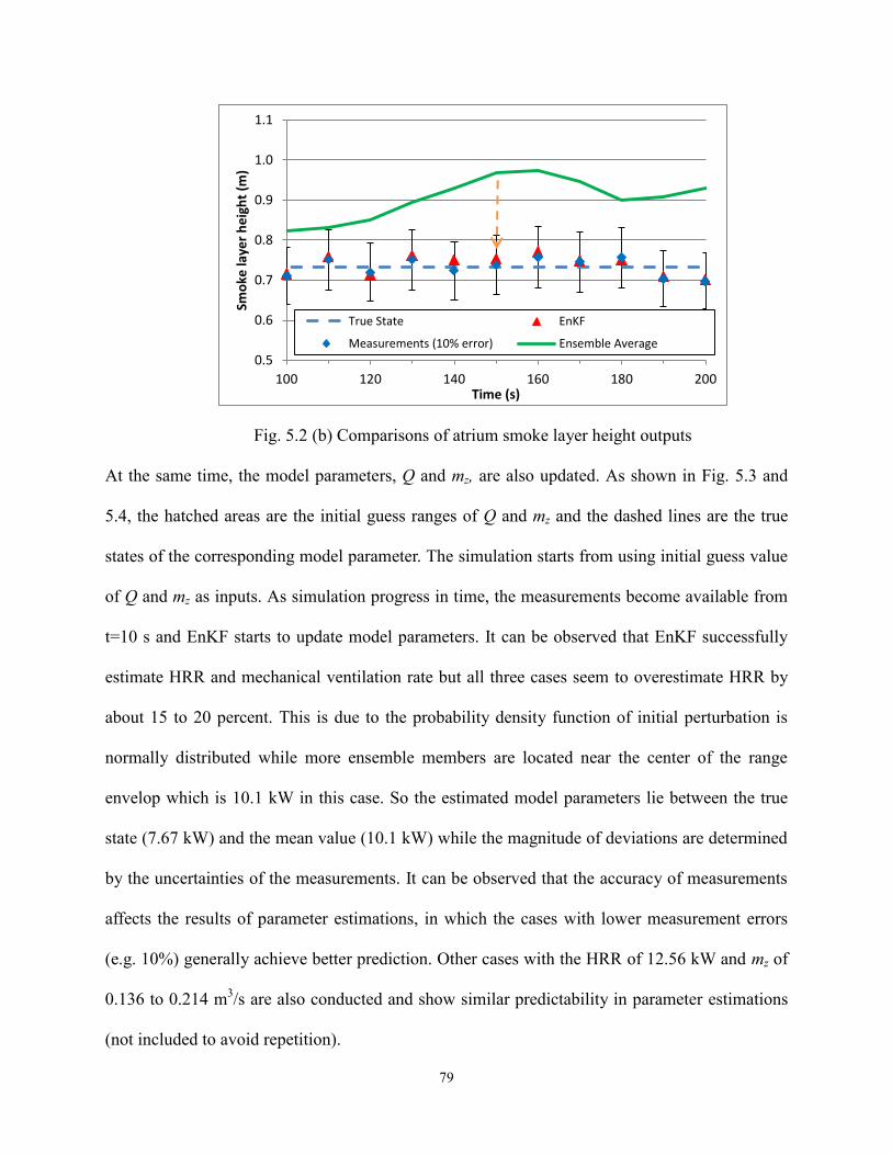
79

Fig. 5.2 (b) Comparisons of atrium smoke layer height outputs

At the same time, the model parameters, Q and mz, are also updated. As shown in Fig. 5.3 and

5.4, the hatched areas are the initial guess ranges of Q and mz and the dashed lines are the true

states of the corresponding model parameter. The simulation starts from using initial guess value

of Q and mz as inputs. As simulation progress in time, the measurements become available from

t=10 s and EnKF starts to update model parameters. It can be observed that EnKF successfully

estimate HRR and mechanical ventilation rate but all three cases seem to overestimate HRR by

about 15 to 20 percent. This is due to the probability density function of initial perturbation is

normally distributed while more ensemble members are located near the center of the range

envelop which is 10.1 kW in this case. So the estimated model parameters lie between the true

state (7.67 kW) and the mean value (10.1 kW) while the magnitude of deviations are determined

by the uncertainties of the measurements. It can be observed that the accuracy of measurements

affects the results of parameter estimations, in which the cases with lower measurement errors

(e.g. 10%) generally achieve better prediction. Other cases with the HRR of 12.56 kW and mz of

0.136 to 0.214 m3/s are also conducted and show similar predictability in parameter estimations

(not included to avoid repetition).

0.5

0.6

0.7

0.8

0.9

1.0

1.1

100 120 140 160 180 200

Smo

ke la

yer

he

igh

t (m

)

Time (s)

True State EnKF

Measurements (10% error) Ensemble Average

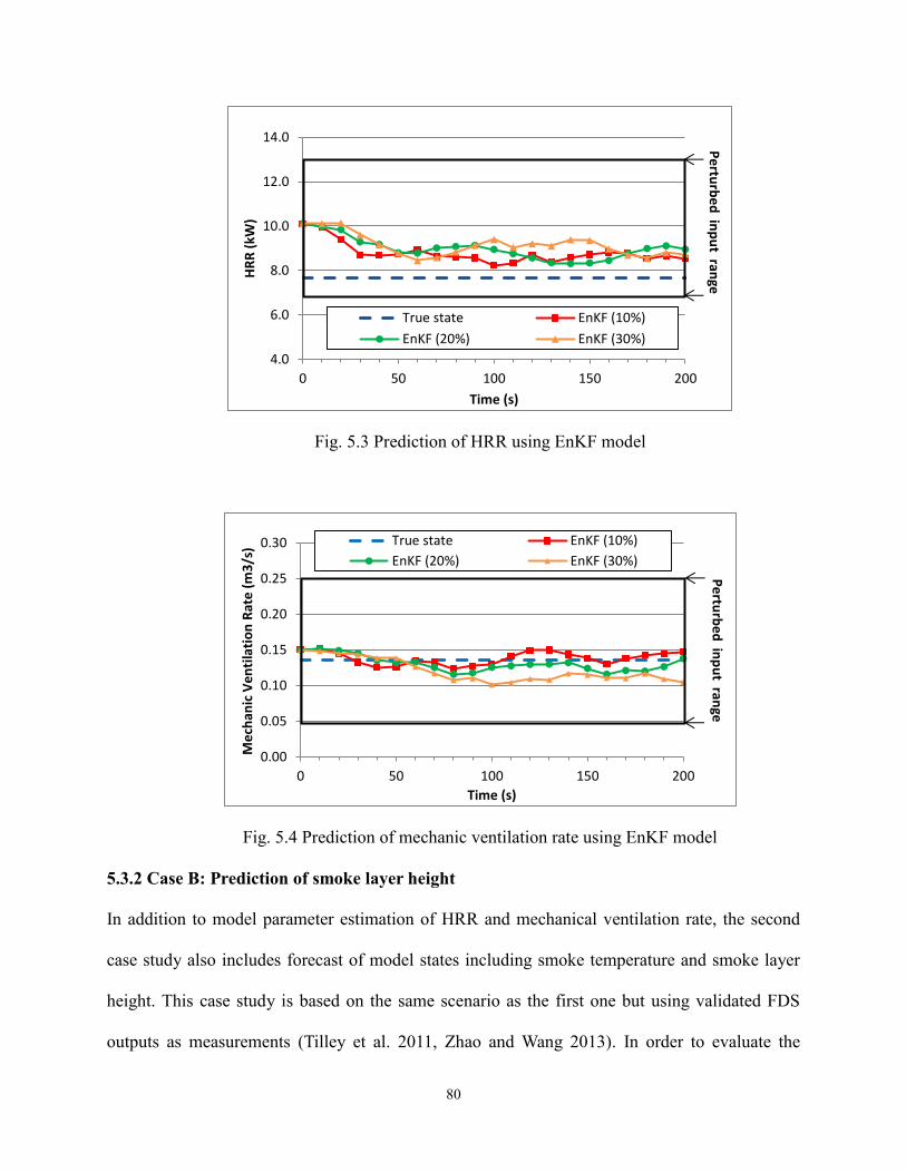
80

Fig. 5.3 Prediction of HRR using EnKF model

Fig. 5.4 Prediction of mechanic ventilation rate using EnKF model

5.3.2 Case B: Prediction of smoke layer height

In addition to model parameter estimation of HRR and mechanical ventilation rate, the second

case study also includes forecast of model states including smoke temperature and smoke layer

height. This case study is based on the same scenario as the first one but using validated FDS

outputs as measurements (Tilley et al. 2011, Zhao and Wang 2013). In order to evaluate the

4.0

6.0

8.0

10.0

12.0

14.0

0 50 100 150 200

HR

R (

kW)

Time (s)

True state EnKF (10%)

EnKF (20%) EnKF (30%)

Pe

rturb

ed

inp

ut ran

ge

0.00

0.05

0.10

0.15

0.20

0.25

0.30

0 50 100 150 200

Me

chan

ic V

en

tila

tio

n R

ate

(m

3/s

)

Time (s)

True state EnKF (10%)

EnKF (20%) EnKF (30%)

Pe

rturb

ed

inp

ut ran

ge

81

EnKF model to predict model states and parameters, the atrium smoke layer height

measurements (hAt) are not given in this case. Instead, it is later used to verify the predictability

of the EnKF model. Based on the FDS simulation results from the previous study Lee et al.

2004), four selected cases are conducted using different combinations of �� and ��𝑧 as shown in

Table 5.2. Although mechanical ventilation rate ��𝑧 is a known input in FDS and can also be

controlled by an operator in the experiment, the actual air mass flow rate through the duct is still

very different from the set point in a compartment fire. It is therefore considered as an unknown

model parameter in this case. The resulting smoke temperature and smoke layer height from FDS

outputs are recorded with 10-second resolution and later used as measurements.

Following the same procedure as Case A, four EnKF simulations are conducted using exactly the

same inputs while the only difference is that the measurement data are based on FDS simulations

in this case. This is similar to forecast an unknown fire while HRR and ventilation rate can only

be roughly estimated in the beginning. After the simulation progress in time, the measurements

become available and are used to adjust the simulation parameters to improve predictability. The

results of B1 case are presented with details in figures and the results of B2, B3 and B4 are

summarized in Table 5.3.

Table 5.2 FDS model inputs and EnKF parameter perturbation ranges of the two-room fire tests

Case # Q (kW) m𝑧 (m3/s)

B1 12.56 0.214

B2 12.56 0.126

B3 7.67 0.136

B4 7.67 0.117

EnKF range 7.1 to 13.1 0.6 to 0.24

Fig. 5.5 demonstrates a comparison of atrium smoke layer height predictions by using different

simulation tools/inputs. Dashed line shows a-priori CFAST simulation by a central ensemble

member using mean values of HRR and mechanical ventilation rate (center of the perturbed

82

range) as inputs while the results are very different from FDS outputs (approximated true state).

It is not surprising that the a-priori CFAST simulation performs poorly because of inappropriate

HRR input, which is used here as a base line for comparison. By using correct inputs (the same

inputs as FDS), the posteriori CFAST results improve but still with some overestimations as

shown by the dashed-dotted line. Finally, the solid line illustrates the results by using EnKF, in

which the inputs of HRR and mechanical ventilation rate are the same as the a-priori simulation

but measurement data are used for data assimilation at every simulation time step (10 seconds)

during the whole simulation. It can be observed that EnKF results are closer to FDS outputs

(solid squares) than the a-priori and a-posteriori CFAST models. Similar results can be found for

other cases as shown in Table 5.3, where all EnKF cases perform better than a-priori CFAST

models. This is due to the fact that EnKF not only estimates model parameters but also adjusts

model states at the same time.

Fig. 5.5 Comparisons of atrium smoke layer height outputs (Case B1)

0.0

0.3

0.6

0.9

1.2

1.5

0 50 100 150 200 250 300

Smo

ke L

aye

r H

eig

ht

(m)

Time (s)

CFAST (a priori) CFAST (a posteriori)

EnKF FDS (approx. true states)

83

Table 5.3 Root mean square errors of atrium smoke layer height prediction by different methods

when compared to FDS simulation results

Case # CFAST CFAST EnKF

A priori (m) A posteriori

(m)

(m)

B1 0.28 0.16 0.08

B2 0.58 0.19 0.23

B3 0.47 0.23 0.17

B4 0.19 0.10 0.13

It can be concluded in this case study that by using EnKF to forecast smoke layer height, the

simulation only requires users to define a reasonable range of HRR and mechanical ventilation

rate. The model is able to estimate model parameters and forecast smoke transport when

measurements become available.

5.3.3 Case C: Forecast smoke spread in a multi-room compartment fire

To further demonstrate the capabilities of EnKF in a more complicated case, the third case study

applies the EnKF model to a five-zone fire simulation. This case study is based on a series of

experiments performed by NIST and has been used to validate FDS and CFAST (Jones et al.

2009, Peacock and Reneke 2007). The test building consists of five compartments including fire

room, corridor, target room and two small spaces connecting mentioned rooms near entrances as

shown in Fig. 5.6. The fire source is a 110 kW constant fire. The doorway connecting the

corridor to the exterior is opened during the whole test.

84

Fig. 5.6 Overview of the five-zone fire test building in FDS

From the validation study of FDS and CFAST, both tools perform well for the rooms close to fire

source (not included here but can be found in McGrattan et al. 2007, Peacock and Reneke 2007).

Fig. 5.7 shows the smoke filling process of the target room in the early stage of the fire by

comparing outputs from different models and experiment measurements. The figure illustrates

that before t = 70 s, it is difficult to measure smoke layer height in the experiment since the

smoke layer is not well developed so the smoke layer height is hard to be determined (McGrattan

et al. 2007). Before t = 70 s, it can be found that both FDS and CFAST outputs are reasonably

close. During the same period, both programs also predict a similar smoke filling process in the

corridor as shown by the SmokeView (Forney 2013) visualization in Fig. 5.8. SmokeView is a

smoke visualization tool developed by the US NIST. At t = 20 s, the smoke starts to propagate

into the corridor along the ceiling then reaches the far end and also gets into the entrance two at t

= 30 s. In general, although the smoke layer of the corridor is formed at about t = 30 s, the

quantity of smoke calculated by CFAST as indicated by the solid line is still reasonable in the

early stage by comparing to that of FDS.

85

Fig. 5.7 Comparisons of target room smoke layer height from experiment measurements

and simulation results

Fig. 5.8 Comparisons of smoke layer height outputs from FDS and CFAST in the corridor

After t = 70 s, more smoke gets into the target room and the smoke layer can be measured

consistently in the experiment (Fig. 5.7). In the meantime, CFAST significantly underestimates

the smoke layer height in the target room. A closer look at the smoke filling process is provided

by Fig. 5.9 where the air temperature is illustrated by different colors as shown by the legends on

the right side. After t = 70 s, the smoke enteris the target room and forms a smoke layer. The

quantity of smoke in the room starts showing differences between CFAST and FDS at t = 70 s.

0.0

0.5

1.0

1.5

2.0

2.5

3.0

0 50 100 150 200 250 300

Smo

ke L

aye

r H

eig

ht

(m)

Time (s)

FDSCFAST_6.3Experiments

t=2

0

t=30

86

Fig. 5.9 Comparisons of smoke layer height outputs in the target room for a fire of 110 kW

At t = 100 s, CFAST starts to further underestimate the smoke layer height and shows significant

difference from FDS outputs. Finally at t = 200 s, the smoke layer height is about 0.11 m from

CFAST while FDS result is around 1 m.

The significant discrepancy of CFAST from FDS simulations of the target room comes from the

CFAST assumptions. In CFAST, each compartment is divided into two layers in which air

properties are assumed to be uniform, and a ceiling jet is not modeled. This method simplifies

calculations but also creates problems in the corridor. Due to momentum effect, more smoke will

exit the corridor through the doorway directly than entering the target room as illustrated in Fig.

5.8. CFAST thus overestimates the mass flow rate through the entrance two as shown in Fig.

5.10. After 70 s, the mass flow rate actually reaches a steady state as illustrated by the dashed

line whereas the CFAST prediction continues to increase till it reaches a value of over two times

more than that of FDS at about 200 s. This explains why the smoke layer height in CFAST is

87

much lower than that in FDS as shown by Fig. 5.9. Although CFAST implemented a delay

function for the smoke spread in a long corridor (Bailey et al. 2002), we tried different delay

functions for the smoke dispersion through the long corridor but the predictability cannot be

improved.

Fig. 5.10 Comparisons of the mass flow rate through the entrance two

This case shows an example how model assumptions affect simulation accuracy. Here we

implement an EnKF-based solution to improving the CFAST simulation. In order to take into

account the forecast uncertainties of the mass flow rate through the corridor doorway, a virtual

sink of mass is added in the corridor to consider excessive mass loss through the door way for

model state correction. The mass sink helps to leverage the mass flows distributed between the

entrance two and the corridor doorway so that the smoke flow through the doorway can be

correctly considered in CFAST. This sink is considered as an uncertainty of 0 to 0.2 m3/s to the

exterior. The range is determined by comparing the FDS and CFAST simulation results to make

sure the perturbed flow rate can cover the true state as illustrated by dotted-arrows in Fig. 5.8.

Regarding other parameter perturbations of the EnKF model, the uncertainty of the fire source

0.00

0.05

0.10

0.15

0.20

0.25

0.30

0.35

0 50 100 150 200 250 300

Flo

w R

ate

(kg

/s)

Time (s)

FDS flow rate

CFAST flow rate

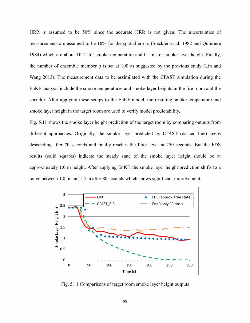
88

HRR is assumed to be 50% since the accurate HRR is not given. The uncertainties of

measurements are assumed to be 10% for the spatial errors (Steckler et al. 1982 and Quintiere

1984) which are about 10°C for smoke temperature and 0.1 m for smoke layer height. Finally,

the number of ensemble member q is set at 100 as suggested by the previous study (Lin and

Wang 2013). The measurement data to be assimilated with the CFAST simulation during the

EnKF analysis include the smoke temperatures and smoke layer heights in the fire room and the

corridor. After applying these setups to the EnKF model, the resulting smoke temperature and

smoke layer height in the target room are used to verify model predictability.

Fig. 5.11 shows the smoke layer height prediction of the target room by comparing outputs from

different approaches. Originally, the smoke layer predicted by CFAST (dashed line) keeps

descending after 70 seconds and finally reaches the floor level at 250 seconds. But the FDS

results (solid squares) indicate the steady state of the smoke layer height should be at

approximately 1.0 m height. After applying EnKF, the smoke layer height prediction shifts to a

range between 1.0 m and 1.4 m after 80 seconds which shows significant improvement.

Fig. 5.11 Comparisons of target room smoke layer height outputs

0

0.5

1

1.5

2

2.5

3

0 50 100 150 200 250 300

Smo

ke L

aye

r H

eig

ht

(m)

Time (s)

EnKF FDS (approx. true state)

CFAST_6.3 EnKF(only FR obs.)

89

Fig. 5.12 shows the results of smoke temperature prediction of the target room by using

difference methods. The solid squares illustrate 10 seconds average of FDS outputs which is

considered as an approximation of the true state and the dashed line is CFAST posteriori

estimation. It can be observed that the smoke temperature is about 15 to 20°C lower than the true

state even though the appropriate HRR is already given. After applying EnKF, the smoke

temperature prediction shifts closer to the solid line after the model states and parameters are

adjusted in the EnKF analysis.

Fig. 5.12 Comparisons of target room smoke temperature outputs

The EnkF simulation in the previous discussion uses the measurements of smoke temperatures

and smoke layer heights in both the fire room and the corridor. In order to demonstrate the

importance of the number of measurements used in EnKF analysis, a case with only fire room

smoke temperature and smoke layer height measurements is also conducted. The results are

illustrated as dash-dotted lines (only FR observation) in Fig. 5.11 and 5.12. It can be observed

that the smoke layer height prediction is worse than the previous case but is still within a

reasonable range of 1.2 m to 1.5 m. But the temperature prediction error is about 20 °C which

0

20

40

60

80

0 50 100 150 200 250 300

Tem

pe

ratu

re (

°C)

Time (s)

EnKF FDS (approx. true state)

CFAST_6.3 EnKF (only FR obs.)

90

accounts for about 28% relative error. This is due to the virtual sink is located in the corridor and

no local measurements in the target room are used in this case so the EnKF model is less

effective than the previous case.

Finally, a comparison of the simulation time and the predictability using three different methods

is presented in Table 5.4. The predictions of smoke temperature and smoke layer height have

significant improvement after applying EnKF. The total simulation time required by EnKF is 520

seconds without using any parallel computing on an Intel 2.8GHz processor while FDS may

require almost an hour to complete with the same hardware. In addition, for the EnkF simulation,

over 80% of computational time is associated with processing the ensemble members

sequentially. Currently, the model requires 520 seconds to perform a simulation of 300 seconds.

If parallel computing is applied to the model to process multiple ensemble members

simultaneously, the model will be potentially able to run in real time for the five-zone

compartment fire prediction.

From a practical perspective, to apply this model to predict fire and smoke dispersion to improve

building fire safety, the HRR of an unknown fire accident can be first estimated by the fuel load

and ventilation conditions of a given space with a reasonable range. When a fire accident occurs

and the fire alarm is activated, the fire source is then assumed to be located in the closest room to

the triggered smoke detector and start taking measurements from the sensors. After the EnKF

analysis, the computer simulations are calibrated with the measurements and generate a more

accurate prediction of fire growth and smoke dispersion which can be used in automated smoke

management, evacuation assistance and decision making in firefighting. For example, the

occupants can follow the signs and avoid going toward toxic smoke while fire fighters can have a

general idea about firefighting strategies before entering the building.

91

Table 5.4 Comparisons of model predictability and CPU time

Temperature

prediction error

Smoke layer

height prediction

error

CPU time

(seconds)

CFAST 28% 53.6% 0.8

EnKF 16.5% 16.5% 520

FDS - - 3330

*The error percentage is based on root mean squared error divided by the average

5.4 Conclusions and future work

A new method to forecast smoke dispersion in a compartment fire by combining state and

parameter estimation is presented. To solve the problems associated with the inaccurate user

inputs and model assumptions, the EnKF model assimilates different types of sensor data such as

smoke temperature and smoke layer height measurements to improve model predictability. The

resulting model is able to forecast long-distance smoke transport from the fire source in a

compartment fire. Comparing to other parameter estimation techniques in compartment fire

simulations that require solving large adjoint matrices, EnKF only needs to operate around 100

ensemble members within a few minutes and can sequentially calibrating the forecast model with

measurement data. The results from three case studies are showing noticeable predictability

while the computational requirement is relatively low.

For those who would apply EnKF to other simulation models, it is suggested to apply a low-

dimensional model with highly accurate short-term forecasts. This is due to the fact that the

EnKF will directly use the simulation model to perform predictions when measurements are not

available. Therefore, simulation tools with lower accuracy with fewer measurements available

will not benefit well from EnKF. In addition, modifications of the simulation tools are sometimes

required. For example in Case C of this study, a virtual sink is added in the corridor to take into

account model limitations due to assumptions. This modification makes the sampling of

92

ensemble members to focus more on most likely errors to improve the model efficiency.

Future studies would require looking into the parameter perturbations and simulation model

convergence criteria. This is due to the fact that, in some cases, when the deviations of model

parameters exceed about 60%, some ensemble members will have difficulty to converge in

CFAST. In addition, spurious correlations should also be looked into since it is a common

problem in all EnKF applications. The case studies presented in this paper are based on buildings

with two to five rooms while all model states are highly-correlated. When the model is applied to

a larger building, the EnKF model should implement a more detailed localization method to

avoid model parameters and states updated with irrelevant measurements such as sensor data

from a room far away from a fire source.

References

Kastner, Wolfgang, Georg Neugschwandtner, Stefan Soucek, and H. M. Newmann.

"Communication systems for building automation and control." Proceedings of the IEEE 93, no.

6 (2005): 1178-1203.

Morari, Manfred, and Jay H Lee. "Model predictive control: past, present and future." Computers

& Chemical Engineering 23, no. 4 (1999): 667-682.

Fux, Samuel F., Araz Ashouri, Michael J. Benz, and Lino Guzzella. "EKF based self-adaptive

thermal model for a passive house." Energy and Buildings68 (2014): 811-817.

Bushby, S. T. "Integrating Fire Alarm Systems with Other Building Automation and Controls

Systems." Fire Protection Engineering 11 (2001): 18-20.

Friedman, Raymond. "An international survey of computer models for fire and smoke." Journal

of Fire Protection Engineering 4, no. 3 (1992): 81-92.

Olenick, Stephen M., and Douglas J. Carpenter. "An updated international survey of computer

models for fire and smoke." Journal of Fire Protection Engineering 13, no. 2 (2003): 87-110.

Babrauskas, Vytenis, and Richard D. Peacock. "Heat release rate: the single most important

variable in fire hazard." Fire safety journal 18, no. 3 (1992): 255-272.

93

Rein, G., C. Abecassis-Empis, A. Amundarain, H. Biteau, A. Cowlard, A. Chan, W. Jahn et al.

"ROUND-ROBIN STUDY OF FIRE MODELLING BLIND-PREDICTIONS USING THE

DALMARNOCK FIRE TEST." In Proceedings of the 5th International Seminar on Fire and

Explosion Hazards, vol. 23, p. 27. 2007.

Lee, Eric WM, Richard KK Yuen, S. M. Lo, K. C. Lam, and G. H. Yeoh. "A novel artificial

neural network fire model for prediction of thermal interface location in single compartment

fire." Fire Safety Journal 39, no. 1 (2004): 67-87.

Richards, R. F., B. N. Munk, and O. A. Plumb. "Fire detection, location and heat release rate

through inverse problem solution. Part I: Theory." Fire safety journal 28, no. 4 (1997): 323-350.

Overholt, Kristopher J., and Ofodike A. Ezekoye. "Characterizing heat release rates using an

inverse fire modeling technique." Fire technology 48, no. 4 (2012): 893-909.

Peacock, R. D., W. W. Jones, P. A. Reneke, and G. P. Forney. "Consolidated Model of Fire

Growth and Smoke Transport (Version 6), User’s Guide." NIST Special Publication 1041.

Koo, Sung-Han, Jeremy Fraser-Mitchell, and Stephen Welch. "Sensor-steered fire

simulation." Fire Safety Journal 45, no. 3 (2010): 193-205.

Hostikka, Simo, and Olavi Keski-Rahkonen. "Probabilistic simulation of fire scenarios." Nuclear

engineering and design 224, no. 3 (2003): 301-311.

Neviackas, Andrew. Inverse fire modeling to estimate the heat release rate of compartment fires.

ProQuest, 2007.

Robinson, Allan R., and Pierre FJ Lermusiaux. "Overview of data assimilation." Harvard reports

in physical/interdisciplinary ocean science 62 (2000): 1-13.

Navon, Ionel M. "Data assimilation for numerical weather prediction: a review." In Data

Assimilation for Atmospheric, Oceanic and Hydrologic Applications, pp. 21-65. Springer Berlin

Heidelberg, 2009.

Evensen, Geir. "Sequential data assimilation with a nonlinear quasi‐geostrophic model using

Monte Carlo methods to forecast error statistics." Journal of Geophysical Research: Oceans

(1978–2012) 99, no. C5 (1994): 10143-10162.

Lin, Cheng-Chun, and Liangzhu Leon Wang. "Forecasting simulations of indoor environment

using data assimilation via an Ensemble Kalman Filter." Building and Environment 64 (2013):

169-176.

Kalman, Rudolph Emil. "A new approach to linear filtering and prediction problems." Journal of

Fluids Engineering 82, no. 1 (1960): 35-45.

McGrattan, Kevin B., Bryan Klein, Simo Hostikka, and Jason Floyd. "Fire dynamics simulator

94

(version 5), user’s guide." NIST special publication 1019, no. 5 (2008): 1-186.

Verlaan, M., Velzen Nv, and S. Hummel. "A generic toolbox for data assimilation in numerical

modeling." In 15th biennial conference of the joint numeric. 2010.

Evensen, Geir. "The ensemble Kalman filter for combined state and parameter

estimation." Control Systems, IEEE 29, no. 3 (2009): 83-104.

Schrader, B. P., and S. F. Moore. "Kalman filtering in water quality modeling: Theory vs.

practice." In Proceedings of the 9th conference on Winter simulation-Volume 2, pp. 504-510.

Winter Simulation Conference, 1977.

Burgers, Gerrit, Peter Jan van Leeuwen, and Geir Evensen. "Analysis scheme in the ensemble

Kalman filter." Monthly weather review 126, no. 6 (1998): 1719-1724.

Tilley, Nele, Pieter Rauwoens, and Bart Merci. "Verification of the accuracy of CFD simulations

in small-scale tunnel and atrium fire configurations." Fire Safety Journal 46, no. 4 (2011): 186-

193.

Jones, W. W., R. D. Peacock, G. P. Forney, and P. A. Reneke. "Consolidated Model of Fire

Growth and Smoke Transport (Version 6): Technical Reference Guide." NIST SP 1026.

Peacock, Richard D., Sanford Davis, and Billy T. Lee. An experimental data set for the accuracy

assessment of room fire models. Center for Fire Research, 1988.

Poreh, Michael, Norman R. Marshall, and Amir Regev. "Entrainment by adhered two-

dimensional plumes." Fire Safety Journal 43, no. 5 (2008): 344-350.

Chang, Shoou-Yuh, and Sikdar MI Latif. "Use of kalman filter and particle filter in a one

dimensional leachate transport model." In Proceedings of the 2007 National Conference on

Environmental Science and Technology, pp. 157-163. Springer New York, 2009.

Wang, Liangzhu Leon, and Guanchao Zhao. "Numerical study on smoke movement driven by

pure helium in atria." Fire Safety Journal 61 (2013): 45-53.

Peacock, R. D., and P. A. Reneke. "Verification and Validation of Selected Fire Models for

Nuclear Power Plant Applications, Volume 5: Consolidated Fire Growth and Smoke Transport

Model (CFAST)." NUREG-1824, US Nuclear Regulatory Commission, Washington, DC (2007).

Forney, Glenn P. Smokeview (version 6) a Tool for Visualizing Fire Dynamics Simulation Data

Volume II: Technical Reference Guide. 2013.

Bailey, J. L., Glenn P. Forney, P. A. Tatem, and W. W. Jones. "Development and validation of

corridor flow submodel for CFAST." Journal of Fire Protection Engineering 12, no. 3 (2002):

139-161.

95

Steckler, K. D., James G. Quintiere, and W. J. Rinkinen. "Flow induced by fire in a

compartment." In Symposium (international) on combustion, vol. 19, no. 1, pp. 913-920.

Elsevier, 1982.

Quintiere, James G., K. Steckler, and D. Corley. "An assessment of fire induced flows in

compartments." Fire Science and Technology 4, no. 1 (1984): 1-14.

96

Chapter 6 Scaled Compartment Fire Experiment

6.1 Background information

Compartment fire experiments have had great success in broadening knowledge of building fires.

However, the cost of a building fire experiment is usually high and the test is not easily

replicated because the building being tested is often damaged by the fire and is not always fully

recoverable. There is additional difficulty creating an identical ambient environment since most

experiments are conducted outdoors in uncontrollable weather conditions. Numerical

experiments (i.e., computer simulations) and scaled fire experiments are alternative ways to

study building fires that are not susceptible to such problems. Although numerical experiments

are widely used and noticeably accurate, the use of computer simulations alone to study a

specific fire phenomenon is not recommended (Johansson 2014). In fact, the only affordable

option for investigating certain types of compartment fire problems such as atrium fires and shaft

smoke transport is scaled fire experimentation. Although the scaling laws that relate small-scale

tests to full-scale results are only applicable to certain types of fuels, building materials, and

compartment geometries (Jolly and Saito 1990; Babrauskas 1995 and 1997), the method can still

give a general picture for predicting smoke temperature and smoke layer height (Moodie and

Jagger 1992).

The goal of the experiment presented in this chapter is to study the effects of changing fire

source HRR and the opening/closing of doors on the smoke filling process of a compartment fire.

These are very common events of real compartment fire accidents. As previously mentioned,

these events are unpredictable, which makes smoke and fire spread difficult to predict. According

to the existing literature, most established fire experiments usually attempt to apply one

97

condition to the entire test to avoid undesirable changes, but this does not produce desirable

results to test dynamical updating of data assimilation. The experiment is specially designed to

study dynamic events during a compartment fire.

6.2 Experiment setups

The experiment setup is a 1:5 scaled building based on a series of experiments conducted by

NIST (Peacock et al. 1988 and 2007). As shown in Fig. 6.1., the scaled building consists of three

rooms. The fire room is built entirely with cement board, except for one wall, which is built with

fire-proof glazing for smoke visualization. The other two rooms are constructed entirely of 0.8

cm-thick acrylic glass. These three rooms are connected by 0.4 m × 0.15 m doors. There are

three doors of the same size in the corridor that lead out of the compartments. Doors 2 and 3 are

closed for most of the tests, while Door 1 remains open.

Fig 6.1 (a) Description of experimental setups

98

Fig 6.1 (b) Experimental setups - apparatus

Table 6.1 Geometries and material properties of the scaled building

Length Width Height Material

Fire room 70 50 50 Acrylic glass

Cement board

Corridor 250 50 50 Acrylic glass

Target room 70 50 50 Acrylic glass

*unit: centimeter

Conductivity

kW/(m K)

Specific Heat

(kJ/kg K)

Density

(kg/m3)

Thickness

(cm)

Acrylic glass 0.0019 1.47 1185 0.8

Cement board 0.29 0.84 1200 1.5

The fire source is a Bunsen burner connected to a propane cylinder whose flow rate is controlled

by a flow meter and is located in the fire room. To prevent oxygen starvation and reduce

experimental uncertainties, the tube to the propane gas supply is fed to the outside air through a

small (0.1 m × 0.1 m) opening in the floor. To obtain the temperature measurement, three

thermocouple trees, each consisting of five type K thermocouples, are installed in each room.

The lowest one is located 5 cm above the floor and the highest one is 45 cm above the floor. The

other three thermocouples are located in-between these two and spaced 10 cm apart, as show in

Fig 6.1. An Agilent 34970A data acquisition unit is linked to all thermocouples and a PC that

99

records measurements every one second.

Since the hot gases in this experiment are generated with high efficiency from a Bunsen burner,

the hot gases are transparent and therefore hard to capture visually. In order to visualize the flow

pattern of the hot gases and observe the smoke layer height, artificial smoke is injected into the

fire room right next to the burner. The injected smoke is generated by a smoke machine that uses

fog fluid to make hot gases visible. To further enhance the effect, the smoke particles are

illuminated by two sheets of green laser light, as shown in Fig 6.2. In addition, the images

captured by digital camera are then analyzed with particle image velocimetry (PIV). Detailed

discussions regarding experiment setups are included in Section 7.1.4.

Fig 6.2 Visualization of smoke layer using artificial smoke and laser light

6.3 Smoke temperature and smoke layer height

The study of the smoke transport process of a compartment fire is based on comparisons of

average smoke temperature and smoke layer height. In this experiment, the temperature

measurements obtained from three thermocouple trees are converted into smoke layer height and

average smoke temperature for easier comparison. The smoke temperature at the interface, T𝐻𝑑,

100

is given by:

T𝐻𝑑 = 𝐶𝑠(𝑇𝑚𝑎𝑥 − 𝑇𝑓𝑙𝑜𝑜𝑟) + 𝑇𝑓𝑙𝑜𝑜𝑟 (6.1)

where 𝑇𝑚𝑎𝑥 is the maximum measured temperature and 𝑇𝑓𝑙𝑜𝑜𝑟 is the temperature measured near

the floor level. 𝐶𝑠 is an empirically determined factor equals to 0.2 (Peacock et. al 1988). The

average smoke layer temperature is determined by the mean integrated temperature measurement

over the layer:

T𝑈 = ∫𝑇(𝑧)

𝐻𝑟𝑜𝑜𝑚𝑑𝑧

𝐻𝑟𝑜𝑜𝑚

𝐻𝑑

(6.2)

where 𝐻𝑑 is the height at which the smoke temperature is T𝐻𝑑 and can be determined by linear

intepolation. 𝐻𝑟𝑜𝑜𝑚 is the height of room. Fig. 6.3 shows an example of converting thermocouple

tree measurements into smoke layer height and smoke temperature. The smoke layer height, or

the interface height, is located where the temperature rise is 20% over the entire room, which is

approximately 0.28 m. By applying Eq. (6.2), the smoke temperature, or the upper layer

temperature, can be determined and is 99.5 °C in this case.

Fig 6.3 Thermocouple measurements and smokelayer height

101

Before testing the effects of dynamic events, a series of tests using the same HRR of 2.0 kW and

door opening setups is conducted to calibrate all equipment. Fig 6.4 shows the temperature

measurements of one thermocople compared to FDS simulation results. The deviations between

the tests are negligible (less than 5%), and the results are also close to FDS outputs. Thus, it can

be confirmed that the experiment is highly repeatable.

Fig 6.4 Comparisons of ceiling thermocouple measurement in the fire room

6.4 Results and discussions

6.4.1 Case A – change of HRR

The heat release rate (HRR) of the fire source is the dominant feature of any compartment fire

(Babrauskas 1992). It is determined by complex chemical reactions that are usually not easily

predictable. In this experiment, the fire source is a Bunsen burner, which makes it much easier to

control. This setup enables comparisons of the effect of fire source HRR on smoke transport.

First, three experiments with constant HRRs are conducted, with values of 1.5, 2.0 and 2.8 kW

based on the propane gas flow rate to the burner. Fig 6.5(a) shows the temperature rise in the fire

room for all cases. The rate of temperature rise is very different for all three cases, even

0

50

100

150

200

250

0 100 200 300 400 500 600

Tem

pe

ratu

re (

∘C)

Time (s)

Fire room top temperature (TC 117)

Test A

Test B

Test C

FDS

102

immediately after ignition of the burner. As expected, the case with higher HRR has a higher rate

of smoke temperature rise. The same phenomenon can be observed in the corridor and target

room, but with approximate 20- and 40-second time delays, respectively, due to the time required

for hot gases to transport to these two non-fire rooms and build up a smoke layer. A comparison

of the temperature rise of the 2.0 kW and 2.8 kW cases in the fire room at t = 100 seconds

reveals a significant temperature difference when the HRR increases by 40% (i.e., from 2.0 kW

to 2.8 kW). A 40% increment may seem high for a well-controlled fire, but for a full-scale

underdeveloped compartment fire in different ventilation conditions, the HRR uncertainties can

be significant especially in the early growth stages (Makhviladze et al. 2006).

Another experiment using non-constant fire is conducted, in which the HRR begins at 1.5 kW

and then changes to 2.8 kW at t = 180 seconds. In Fig 6.5(a), the purple contour shows a sudden

temperature rise at around 180 seconds in the fire room due to the change of fire HRR. The

sudden temperature rises of the other two rooms have similar time delays of 20 to 40 seconds.

While strong correlations were found between average smoke temperature and HRR, the

correlations between smoke layer height and HRR are much weaker, as shown by Fig 6.6. The

smoke layer height contours obtained from temperature measurements in the fire room are nearly

identical. Similar results can be found from the corridor measurements. But, for the higher HRR

case (2.8 kW), the smoke layer descends faster in the early stage due to the fire source’s higher

flow rate. After around 120 seconds, once the same layer is well-developed in the corridor, all

three cases show nearly identical smoke layer height.

103

Fig 6.5 Comparisons of average smoke temperature rise in three rooms

0

50

100

150

200

0 100 200 300 400 500

Tem

pe

ratu

re (

∘C)

Time (s)

(a) Fire room smoke temperature rise

1.5 kW 2.0_kW

2.8 kW 1.5 kW to 2.8 kW

0

5

10

15

20

25

0 100 200 300 400 500

Tem

pe

ratu

re (

∘C)

Time (s)

(b) Corridor smoke temperature rise

1.5 kW2.0 kW

2.8 kW1.5 kW to 2.8 kW

0

1

2

3

4

5

0 100 200 300 400 500

Tem

pe

ratu

re (

∘C)

Time (s)

(c) Target room smoke temperature rise

1.5 kW2.0 kW2.8 kW1.5 kW to 2.8 kW

104

Fig 6.6 Comparisons of smoke layer height in three rooms

0

0.1

0.2

0.3

0.4

0.5

0 100 200 300 400 500

Smo

ke la

yer

he

igh

t (m

)

Time (s)

(a) Fire room smoke layer height

1.5 kW 2.0_kW

2.8 kW 1.5 kW to 2.8 kW

0

0.1

0.2

0.3

0.4

0.5

0 100 200 300 400 500

Smo

ke la

yer

he

igh

t (m

)

Time (s)

(b) Corridor smoke layer height

1.5 kW 2.0 kW

2.8 kW 1.5 kW to 2.8 kW

0

0.1

0.2

0.3

0.4

0.5

0 100 200 300 400 500

Smo

ke la

yer

he

igh

t (m

)

Time (s)

(c) Target room smoke layer height

1.5 kW

2.0 kW

2.8 kW

1.5 kW to 2.8 kW

105

For the target room smoke layer height, it is necessary to check the near-ceiling thermocouple

measurements to determine the time at which the hot gases enter the room. Fig 6.7 indicates that

the air temperature rise near the ceiling is first detected at 30 seconds after ignition of the burner

in the 2.8 kW HRR case. For the 2.0 kW and 1.5 kW HRR cases, hot gases reach the target room

at 36 and 42 seconds, respectively. This is due to the higher HRR fire sources also generate more

mass/volume of hot gases. In other words, the flow speed is higher and the time required to reach

the target room is shorter for high HRR cases. By obtaining the average travel time of smoke

reaching the target room, the observations at the time when no smoke enters the target room can

be excluded.

Fig 6.7 Temperature rise of target room ceiling thermocouple measurement

Fig 6.6(c) shows that, in general, in the case with higher HRR, the smoke layer descends faster in

all three rooms. But, for the non-constant HRR case, the smoke layer height rises after HRR is

increased from 1.5 kW to 2.8 kW. This can be explained by comparing the temperature profiles

at different times. Fig 6.8 illustrates the temperature profile in the target room at 150, 200 and

250 seconds after ignition. Originally, the temperature profile at 150 seconds, as shown by the

0

1

2

3

4

0 20 40 60 80 100

Tem

pe

ratu

re (

∘C)

Time (s)

Target room ceiling TC temperature rise

1.5 kW

2.0 kW

2.8 kW

106

blue contour, is a smooth curve using 1.5 kW HRR. When the HRR changes to 2.8 kW at 180

seconds, hotter gases start entering the room at around 200 seconds and change the temperature

profile, which creates a steep temperature rise above 0.25 meters height, as shown by the green

contour. This change also results in the rise of the smoke layer height at 200 seconds. As the

hotter smoke generated by the 2.8 kW fire keeps entering the room, the lower layer air is heated,

as shown by the purple contour, and the smoke layer height starts descending. Finally, the

temperature profile changed back to its original smooth shape only when measured at

temperatures higher than those measured at 150 seconds.

Fig 6.8 Target room temperature profiles at different time (HRR = 2.0 kW)

6.4.2 Case–B - change of opening

In addition to fire source HRR, the location and size of compartment openings also affect smoke

transport, especially when the openings are near the fire source. These openings not only provide

paths for smoke spread but also bring in additional air, which nurtures fire development. In

closed compartments, or ones with very small openings, the fire becomes ventilation-controlled

and limited by the quantity of oxygen available. In this experiment, the fire source always has a

0

0.1

0.2

0.3

0.4

0.5

0 1 2 3 4

He

igh

t (m

)

Temperature rise (degC)

Target room temperature rise

t=150

t=200

t=250

107

sufficient oxygen supply, so the opening only affects the transport of hot gases.

Table 6.2 shows three experimental setups with different door locations, as illustrated in Fig 6.1.

The results of average smoke temperature rise are shown in Fig 6.9. Because the fire room is

well-ventilated, the locations of the openings have very little effect on the fire room smoke

temperature. For corridor smoke temperature, represented by the red contour in Fig 6.9(b), Case

1 shows the highest temperature rise of all three cases. This is because Door 1 is located at the

end of the corridor that is furthest from the fire room, and the hot gases that flow out of this

opening have the lowest temperature. In other words, the total energy loss through the opening is

relatively lower for Case 1. Overall, the results indicate that the door position has only a minor

effect on the smoke temperature and smoke layer height. This may be due to the fact that the fire

source is a Bunsen burner, and the flow rate change is relatively small comparing to the air

supplied by the fire room floor opening.

Table 6.2 Door position for three case setups

Door 1 Door 2 Door 3

Case 1 Open Closed Closed

Case 2 Closed Open Closed

Case 3 Open Closed Open at t = 180 s

108

Fig 6.9 Comparisons of smoke temperature rise in three rooms for different door setups

0

30

60

90

120

0 100 200 300 400 500

Tem

pe

ratu

re (

∘C)

Time (s)

(a)Fire room smoke temperature rise

Case 1 (door 1)

Case 2 (door 2)

Case 3 (door 1 and 3)

0

5

10

15

0 100 200 300 400 500

Tem

pe

ratu

re (

∘C)

Time (s)

(b) Corridor smoke temperature rise

Case 1 (door 1)

Case 2 (door 2)

Case 3 (door 1 and 3)

0

1

2

3

4

0 100 200 300 400 500

Tem

pe

ratu

re (

∘C)

Time (s)

(c) Target room smoke temperature rise

Case 1 (door 1)

Case 2 (door 2)

Case 3 (door 1 and 3)

109

Fig 6.10 Comparisons of smoke layer height in three rooms for different door setups

0

0.1

0.2

0.3

0.4

0.5

0 100 200 300 400 500

Smke

laye

r h

eig

ht

(m)

Time (s)

(a) Fire room smoke layer height

Case 1 (door 1)Case 2 (door 2)Case 3 (door 1 and 3)

0

0.1

0.2

0.3

0.4

0.5

0 100 200 300 400 500

Smo

ke la

yer

he

igh

t (m

)

Time (s)

(b) Corridor smoke layer height

Case 1 (door 1)Case 2 (door 2)Case 3 (door 1 and 3)

0

0.1

0.2

0.3

0.4

0.5

0 100 200 300 400 500

Smo

ke la

yer

he

igh

t (m

)

Time (s)

(c) Target room smoke layer height

Case 1 (door 1)Case 2 (door 2)Case 3 (door 1 and 3)

110

References

Babrauskas, Vytenis, and Richard D. Peacock. "Heat release rate: the single most important

variable in fire hazard." Fire safety journal 18, no. 3 (1992): 255-272.

Peacock, Richard D., Sanford Davis, and Billy T. Lee. An experimental data set for the accuracy

assessment of room fire models. Center for Fire Research, 1988.

Peacock, R. D., and P. A. Reneke. "Verification and Validation of Selected Fire Models for

Nuclear Power Plant Applications, Volume 5: Consolidated Fire Growth and Smoke Transport

Model (CFAST)." NUREG-1824, US Nuclear Regulatory Commission, Washington, DC (2007).

Johansson, Nils. "Numerical experiments and compartment fires." Fire Science Reviews 3, no. 1

(2014): 1-12.

Babrauskas, Vytenis. "The generation of CO in bench‐scale fire tests and the prediction for real‐scale fires." Fire and Materials 19, no. 5 (1995): 205-213.

Babrauskas, Vytenis. "Sandwich panel performance in full‐scale and bench‐scale fire tests." Fire

and materials 21, no. 2 (1997): 53-65.

Moodie, K., and S. F. Jagger. "The King's Cross fire: results and analysis from the scale model

tests." Fire Safety Journal 18, no. 1 (1992): 83-103.

Jolly, Shashank, and Kl Saito. "Scale modeling of fires with emphasis on room flashover

phenomenon." Fire safety journal 18, no. 2 (1992): 139-182.

Makhviladze, G. M., A. V. Shamshin, S. E. Yakush, and A. P. Zykov. "Experimental and

numerical study of transient compartment fires. "Combustion, Explosion and Shock Waves 42,

no. 6 (2006): 723-730.

111

Chapter 7 Forecasting Smoke Transport in Real-Time

The models presented in Chapters 5 and 6 focus on a posteriori estimation of model states and

important parameters. In this chapter, the model is designed to be calibrated with a bench-scale

fire experiment and to predict smoke transport using real-time measurements.

7.1 Potential problems and important EnKF model parameters

The performance of an EnKF model heavily depends on several important model parameters to

determine simulation and observation error covariance and to further estimate the approximated

true states of the system. These parameters also directly affect simulation accuracy and speed. In

addition, when applied to a forecasting simulation of building environment, the determination of

these parameters can be very different from that of other types of systems. This section discusses

the potential problems that can arise when these EnKF model parameters are not properly

defined, as well as possible solutions for overcoming these problems.

7.1.1 Localization and spurious correlation

In general, the physical states of two different locations that are near each another are usually

highly correlated. In contrast, there is very little correlation between the physical states of two

locations that are physically far away from each other; thus, such correlations are considered

spurious. In other words, potential problems may arise when all observations are equally applied

to an EnKF analysis. For a compartment fire scenario as presented in this chapter, the

correlations between the observations and model states should take into account the flow rate

between the rooms. To well illustrate the problems for the reader’s convenience, we start again

with the basic equations of EnKF.

X𝑎 = 𝑋𝑓 + K(𝑦 − 𝐻𝑋𝑓 ) (7.1)

112

𝐾 =𝑃𝑓𝐻𝑇

𝐻𝑃𝑓𝐻𝑇 + 𝑅 (7.2)

If the spurious correlations are not considered when observing Eq. (7.1) and Eq. (7.2), the

measurement innovation (difference between measurement and forecasted measurement)

y − HX𝑓 becomes equally important to any model state regardless of the distance between them

because 𝐻𝑃𝑓𝐻𝑇 + 𝑅 is constant for one specific measurement. This may cause a model state to

be updated with an irrelevant observation even when the noise is much greater than the

correlation (Hamill et al. 2001). To account for this issue, various measures, which are so-called

“localization methods”, are proposed based on modifying forecasted error covariance 𝑃𝑓 and

observation error covariance R in Eq. (7.2). For example, for the grid points that are far away

from the observation location, the correlation becomes weaker where 𝑃𝑓should approach zero.

This can also be interpreted that when K is approaching zero in Eq. (7.2), the optimal model

states, X𝑎, in Eq. (7.1) are solely dependent on the forecasted states, 𝑋𝑓. Another method for

achieving a similar effect is to increase the measurement error covariance, R. By increasing R

when the distance is greater, the uncertainty of the measurement becomes higher, and the signal

becomes relatively lower. Thus, when R increases, K approaches zero, which yields similar

results to localizing 𝑃𝑓.

In order to formulate localization methods, Houtekamer and Mitchell (2001) introduced a

distant-dependent reduction of background (simulation) error covariance method for an EnKF.

The simulation error covariances are localized by applying a Schur-product based on a distant-

dependent function where the Schur-product, ρ, for covariance localization is determined by:

ρ = −1

4𝑑5 +

1

2𝑑4 +

5

8𝑑3 −

5

3𝑑2 + 1 𝑓𝑜𝑟 0 ≤ 𝑑 ≤ 1 (7.3)

113

ρ =1

12𝑑5 −

1

2𝑑4 +

5

8𝑑3 +

5

3𝑑2 − 5d + 4 −

2

3∙

1

𝑑𝑓𝑜𝑟 1 ≤ 𝑑 ≤ 2 (7.4)

ρ = 0 𝑓𝑜𝑟 2 ≤ 𝑑 (7.5)

d =|𝑧|

𝑐 (7.6)

where z is the physical distance between model grid points or the distance between the observed

location and a grid point, and c is the distance to scale the correlations between two nodes. The

correlation is assumed to be 1.0 when the distance is below c and gradually reduced to 0 when

the distance is increased to 2c. For the smoke transport forecasting model presented in this

chapter, c is determined by the average travel distance of hot smoke gases during a time period

between two measurements. For example, the average velocity at the fire room door is 0.4 m/s

(will be discussed in Section 7.1.3) with a 10-second sensor resolution. By applying Eq. (7.3) to

Eq. (7.6), the localization factor from the fire room to the corridor is about 0.15. For a system

with n model nodes and m observations, ρ is an n by m matrix, which is the same as the

dimension of K. Therefore, the Kalman gain can be improved by the Schur-product where

K𝑒 =(ρ ∘ 𝑃𝑓)𝐻𝑇

𝐻(ρ ∘ 𝑃𝑓)𝐻𝑇 + 𝑅 (7.7)

Fig 7.1 shows a comparison of the smoke layer height prediction in the target room using two

different EnKF models. All input parameters are identical except that one case uses improved

Kalman gain by applying the localization method as shown by Eq. (7.7), while the other uses

unimproved Kalman gain. As shown by the dotted orange line, the observation is given from

t = 10 to t = 100 seconds to update model states. Although local measurements are also given,

the results still show high deviations between the EnKF outputs and the measurements. This is

because the EnKF over-predicts the error covariance between the predicted target room smoke

layer height and the measurements from rooms far away. These correlations are supposed to be

114

weakly correlated due to their long distances but are mistaken as highly correlated in this case.

These spurious correlations update target room smoke layer height inaccurately. Since the

posteriori estimations of the target room smoke layer height are not successful in this case, the

predicted smoke layer height from t = 100 to t = 500 seconds, as shown by the solid-orange

line, is also very different from the experiment results and even worse than direct simulation

using the zone model. By applying the aforementioned localization methods, as shown by the

purple contour, the model reasonably performs posteriori estimation and also predicts the smoke

layer height from t = 100 seconds and t = 500 seconds with noticeable accuracy.

Fig 7.1 Comparison of EnKF results using localized and non-localized Kalman gain

7.1.2 Filter divergence

As mentioned in the previous section, the accuracy of an EnKF model is based on the estimation

of simulation and observation covariances using a limited number of ensemble members. When

the EnKF parameters are not appropriately defined, the model may have difficulty determining

analysis states (approximate true states), which causes filer divergence. A very commonly found

problem that causes filter divergence is when the perturbation range of the ensemble members

0

0.1

0.2

0.3

0.4

0.5

0 100 200 300 400 500

Smo

ke la

yer

he

igh

t (m

)

Time (s)

Target room smoke layer height

Experiment

Direct simulation

EnKF localized

EnKF non-localized

115

does not cover the true state of the system. As illustrated by Fig 7.2, when the true state acts like

one of the ensemble members, the sampling strategy is considered good because the error of the

model parameter can be determined and used to improve the model. However, when the true

state is not included in the ensemble perturbation range, the model may have difficulty

determining a proper value since all ensemble members are incorrect.

Fig 7.2 Illustrations of ensemble sampling strategies

There are several possible solutions for ensuring the ensemble perturbations covering the true

state. The first method is to increase the number of ensemble members to enlarge the

perturbation range. Since the perturbation of initial parameters is normally distributed, increasing

the number of ensemble members will likely widen the upper and lower perturbation boundaries.

However, this method is considered computationally intensive and inefficient when applied to a

high dimensional system (when the number of model states, n, is much greater than the number

of ensemble members, q).

The second method is to perturb the initial states of the simulation model to increase the range of

ensemble member outputs. This method only works for cases with a high accuracy simulation

model. For the simulation models with lower accuracy and higher systematic errors (higher bias),

filter divergence will still occur when the simulation progresses over time and all ensemble

members are going in the wrong direction, as shown in Fig 7.2. In this case, it is suggested to

116

apply the third method by adding a zero-mean white noise to the simulation model at every

analysis cycle to provide more spread to the ensemble members. This method is especially

suitable for mass transport problems when the model nodes are far away from the source

location. This is due to the model states are nearly identical for all ensemble members at these

far-away nodes in the early stage of simulation. The major drawback of this method is that more

ensemble members are required to compensate for the additional white noises in order obtain

accurate simulation error covariance. As a result, the additional numerical operations required to

process ensemble members in EnKF analysis cycles directly affect computational time and are

especially critical for systems that are designed to perform forecasting in real time. Therefore,

the forth method can be applied to avoid filter divergence is setting up a threshold or a switch to

start EnKF analysis. For example, in the case of a compartment fire, this can be a certain degree

of increase in temperature rise detected from near-ceiling thermocouples. For instance, at the

early stage of the fire, when there are no hot gases entering the rooms located far away from the

fire source, the measurements taken from those sensors located in faraway rooms are still at the

same initial ambient temperature. Thus, it is not necessary to process Kalman gain and update the

model states. By setting up a threshold, the EnKF model not only avoids filter divergence but

also bypasses unnecessary numerical operations.

In order to select an appropriate method for overcoming filter divergence problems, it is

suggested that one use current available measurements to do a posteriori estimation and evaluate

the discrepancies between the direct simulation results and the measurements. Based on general

estimations of errors for each parameter, the parameters to be perturbed can be selected, and the

magnitude of the perturbation can also be generally determined.

117

7.1.3 Determination of measurement uncertainties R

Measurement uncertainties are expected errors of the measurements obtained from the apparatus,

so the uncertainties are either from the device itself or the interpretation of an indirect

measurement. The measurements that are used in the EnKF analysis in this chapter are obtained

from the experiment presented in Chapter 6. The thermocouples and data logger are calibrated

before each set of experiments and are, therefore, considered highly accurate. In addition, the

measurements obtained from repeating bench-scale experiments in the previous chapter show

very minor deviations and are thus considered precise. By excluding the possible errors from the

experiment apparatus, the uncertainties of the measurements are mostly dependent on zonal

deviations. Because the smoke temperature and smoke layer height of a given room are

calculated from the measurements of one thermocouple tree where the zonal deviations are

excluded, they can be considered as indirect measurements. In general, the hot gases inside a

room can deviate significantly depending on the location, especially in the early stage of fire. As

illustrated by Fig 7.3, the zonal deviation of the gas temperature near the ceiling can be up to 20

°C in this case. In order to determine the uncertainties, an FDS model is employed, using the

bench-scale experiment setups as inputs, and R is approximated by the FDS outputs. For

example, the smoke layer height uncertainties in the fire room are 10% of the room height, and

the temperature uncertainties are 10% of the average smoke temperature rise in the early stage

(i.e., first 30 seconds); then, both decrease to 5% when the hot gas layer is well-developed. The

measurement uncertainties of the corridor are assumed to be 20% in the early stage and 10%

later on due to its larger size and higher zonal deviation. These uncertainties are considered

independent, so the error covariances among different locations are assumed to be zero.

118

(°C)

Fig 7.3 Zonal temperature distribution of the fire room from FDS results

7.1.4 Ensemble perturbation strategies

The major advantage of using EnKF to forecast building environment is that the important model

parameters can be adjusted when measurements are available. By using more accurate model

parameters, the predicted physical conditions can maintain at a desired accuracy in a longer time

window. Therefore, in order to have an efficient EnKF model, it is important to select the

parameters to be perturbed and design the magnitude of perturbation.

The most important parameter for a zone model simulation is HRR of the fire source. Since the

flow rate of the fire plume is also based on a sub model using HRR as input, HRR directly

affects both energy and mass conservation equation which makes it the most important parameter

that determines model accuracy. Another parameter that determines the accuracy of the zone

model is the door flow rate. As mentioned in Chapters 5 and 6, the main reason that a zone

model fails to predict smoke transport to rooms distant from the fire source is the accumulating

errors of the door flow rates. Therefore, it is suggested to add a new parameter to adjust flow rate

at the corridor door. Detailed discussions are included in Chapter 5 so it is not presented here to

avoid repetition.

In previous chapter, the inspection of the smoke layer height is based on injecting artificial

119

smoke and projecting laser sheets to visualize the hot gases layer. The visualized smoke layer

height is close to the results interpreted from temperature measurements and also FDS simulation

results. In this chapter, a detailed analysis of flow field is required to determine the uncertainties

of the zone model flow rates. An initial test of using artificial smoke as seeder in a particle image

velocimetry (PIV) system is conducted. The result shows that the lower layer does not have

sufficient seeders for flow field visualization due to the buoyancy of the hot gases as show in Fig

7.4. In this case, the injected seeder is replaced by aluminum oxide powder (Al2O3). Although

the particles of aluminum oxide powder are with small size (10 μm or smaller), the images

obtained from PIV system are showing promising results where the particles are distributed all

over the compartment as shown in Fig 7.5.

Fig 7.4 Flow field visualization using artificial smoke

Fig 7.5 Flow field visualization using aluminum oxide powder (Al2O3)

120

From the experience gained from Chapter 5, the uncertainties of mass flow rate through doors

should be included in the ensemble perturbation. Therefore, the PIV tests are conducted at the

center line of the fire room door to estimate the average mass flow rate. As shown in Fig 7.6, the

flow direction changes rapidly due to the turbulence near the door. In addition, the results are

showing high deviations when repeating the same test setups. In order to obtain an average flow

velocity, it can be achieved by either recording images from multiple planes altogether or

repeating the test and photographing different planes. However, the small door size does not

allow the prior method because the laser sheets are too close to each other so the particle images

can be noisy. The latter method is also not reliable since the unstable flow direction. Therefore,

the PIV tests are conducted near the center of the corridor where the flow pattern is more stable

and can be easily analyzed. Following are the general experiment setups of the PIV system.

(a) Seeding

The seeding particles are based on ceramic material Al2O3 which are injected near the burner and

the corridor section. The advantage of using Al2O3 over artificial smoke is its endurance to high

gas temperature such as the heat generated by the propane burner. The diameter of the particle is

less than 10 μm and the density is around 4g/cm3. The seeding process is based on global seeding

method (Melling 1997) because the hot gas flow rate from the fire room to the corridor is

relatively high and the corridor can be well-seeded in the early stage of fire. In order to inject the

particles in a more stable flow rate, the seeders and air are pre-mixed in a special seeding

chamber (30 cm x 30 cm x 30 cm, 3mm-thick acrylic) before entering the experiment

compartments. The angle of the injection is adjusted to avoid interferences to the burner and the

corridor flow field.

(b) Laser

121

The projected laser for particle visualization is based on a Nd:YAG laser machine (Newwave

solo) which can perform 15-200 mJ output at 532 nm. The laser is projected through a cylindral

lens attached in front of the laser beam while the projected laser is converted to a sheet to

illuminate the plane of interest for particle visualization. The frequency of the laser pulses is

adjusted by the software Flowmanager©

according to the rate of images are captured by the

digital camera.

Fig 7.6 Flow velocity field at fire room door from PIV results

Fig 7.7 Location for images taken for PIV analysis

122

(c) Camera

The images of illuminated particles are captured by a fast speed CCD digital camera using

Nikkor 35mm F2 lens. The calibration are also based on Flowmanager©

including the adjustment

of lens focus and length scale of the image to pixels.

(d) Image process

The images taken from the camera are divided into multiple integration areas (32 by 32 or 64 by

64) where the size of each integration area should be greater than 1/4 of the particle travel

distance during an image capturing time interval. The resulting images are first processed by

cross-correlations and average filtering. Finally, the detailed statistics of all vectors of the flow

field can be generated.

Fig 7.8 shows a comparison between the flow fields of FDS and of PIV. The length of the vectors

illustrates the flow velocity at different location. Both flow fields are separated into two zones

where the upper part is a hot gas zone with its flow direction to the right and the lower part is a

cold air zone with its flow direction to the left. Two zones are separated by the red lines where

the air velocity is assumed zero. It can be observed that FDS outputs have a smaller hot gas zone

but the velocity is relatively higher. By multiplying the cross-section areas for both cases, the

volume flow rates are very close for both cases. Thus, the flow rates in the experiment may be

approximated by the FDS results including the door flow rate. Finally, the uncertainties of the

zone model flow rate are approximated by comparing zone model and FDS results.

123

Fig 7.8 Comparisons of flow velocity field at t = 20 seconds

The perturbations of HRR and mass flow rate through corridor opening are based on the

Gaussian distribution where the expected value and standard deviations are prescribed in the

EnKF model. Fig 7.10 shows an example of HRR perturbation using the Gaussian distribution

where 68% of the ensemble members are expected to be within the range of Qf ± σ where Qf is

2.0 kW and σ is 0.75 kW. Similar method is also applied to the perturbation of mass flow rate

through the corridor opening where σ is 0.01 kg/s which is approximated by the comparisons of

zone model and FDS results. This is due to the flow field at the door is relatively more noisy in

PIV outputs so the reference flow rates are based on FDS results.

124

Fig 7.9 Comparisons of flow velocity field at t = 70 seconds

Fig 7.10 Probability distribution of HRR perturbation based on the Gaussian distribution

125

7.1.5 Number of ensemble members

To achieve real-time prediction, the time for processing one EnKF analysis cycle should be

shorter than the time period between two available measurements. In general, more than 80% of

the computational time of EnKF numerical operations relates to processing ensemble members.

Therefore, the number of ensemble members is the most important parameter in balancing the

model accuracy and simulation speed.

Fig 7.11 shows the comparisons of forecasting errors using different numbers of ensemble

members when the measurements are provided for the first 100 seconds with 10-second time

intervals. The blue contour with triangle (200-second forecast) means the model predicts the

smoke transport for 200 seconds after the measurements stop being provided. The y-axis (RMSE

%) is the average root mean square error (RMSE) of the forecasted smoke temperature divided

by the average smoke temperature.

The values presented in the figure are the average of seven simulations, while the cases with the

highest and lowest RMSE are excluded. It can be observed that the RMSE % decreases

drastically when the number of ensemble members increases from 5 to 20 for both, 200-second

and 400-second, cases. After that, the results show no significant improvement in the

predictability of smoke temperature. Similar results can be found in Fig 7.11(b) for the

forecasted error of the smoke layer height from q = 5 to q = 20. But, the RMSE % keeps

decreasing when q increases from 20 to 40, which indicates that the model with 40 ensemble

members performs better at predicting smoke layer height in this specific case.

126

Fig 7.11(a) Comparisons of temperature forecasting error using different numbers of q

Fig 7.11(b) Comparisons of smoke layer height forecasting error using different numbers of q

*RMSE% is defined as RMSE divided by the mean

To process 100-second available measurements and forecast smoke transport for 400 seconds,

this model requires about seven seconds of computational time, which is less than the

measurement time interval of 10 seconds. Therefore, 40 ensemble members can be considered an

optimal number for balancing forecast accuracy and CPU time, while achieving the goal of real-

15

17

19

21

0 10 20 30 40 50 60

Tem

pe

ratu

re R

MSE

(%

)

Number of ensemble member q

200-second forecast

400-second forecast

15

20

25

30

35

0 10 20 30 40 50 60

Smo

ke la

yer

he

igh

t R

MSE

(%

)

Number of ensemble member q

200-second forecast

400-second forecast

127

time forecasting.

Compared to the model presented in Chapter 5, this model requires a lesser number of ensemble

members to achieve desirable predictability in forecasting smoke transport. This is because

previous models are based on existing tools – CFAST 6.3 and OpenDA 1.1, making it more

difficult to implement localization methods. The spread of ensemble member outputs is based on

adding white noises; thus, more ensemble members are required to achieve similar predictability.

7.2 Forecasting smoke transport in a compartment fire

This section includes two different types of forecasting. The first type is forecasting a

compartment fire with constant HRR, and the second type is with non-constant HRR. The model

parameters are tested with a set of 2 kW HRR experiment results that show noticeable

predictability. After that, the model is directly applied to forecast other cases with different

observation data using exactly the same model parameters.

7.2.1 Forecasting smoke transport with constant HRR source

Case A – 1.5 kW fire

The first case is based on a 1.5 kW fire, in which observations are given every 10 seconds. In

order to test the predictability of the EnKF model, three different tests are conducted, wherein the

measurements are provided for the first 50, 100 and 150 seconds respectively. As shown in Fig

7.12, the red dashed lines are the results of direct simulation using a zone model and the blue

solid lines are the experiment results. It can be observed that the zone model over-predicts smoke

temperature in all three rooms, especially in the early stage of a fire. This may be because the

lower layer is considered adiabatic in the model assumption, so the total energy entering the

upper layer is over-estimated, resulting in high temperatures. This effect is especially noticeable

128

in the early stage of the fire since the lower layer volume is much greater than the upper layer.

After applying the EnKF model, the posteriori estimations of the smoke temperature and smoke

layer height (represented by dotted lines) are adjusted based on available measurements in the

EnKF analysis. At the same time, the perturbed model parameters (i.e., HRR and door flow rate)

are also estimated and used to forecast smoke transport. For example, the solid green line in Fig

7.12(f) shows the forecasted smoke layer height in the target room. When the measurements stop

being provided, at t = 50 seconds, measurements from the fire room and the corridor are used,

and the forecasted smoke layer height shows minor improvement since the local measurements

in the target room are still noisy. In addition, the updated HRR and flow rate estimations help

improve forecasting simulation results when measurements are not available. Following the same

procedures when measurements are provided up to t = 100 seconds, as indicated by the purple

dotted line, the posteriori estimation shows significant improvement when local measurements

are available. After t = 100 seconds, when the measurements become unavailable, the forecasted

smoke layer height still maintains reasonable accuracy, and finally, at t = 150 seconds, when

more measurements are available, the model accurately predicts the smoke layer height in a

longer time window because the model parameters have been corrected.

When comparing the forecasted smoke temperature and smoke layer height in different rooms,

the results in the corridor show greater discrepancy between the forecasted states and the

measurements. This is because the volume of the corridor is much greater than that of the other

two rooms; thus, a higher measurement error as discussed in Section 7.13, is assigned to R to

account for zonal deviation. When measurement uncertainties of the corridor are taken into

account, the predicted smoke layer height and smoke temperature are still within a reasonable

range as defined by R.

129

0

50

100

150

200

0 100 200 300 400 500

Tem

pe

ratu

re (

de

gC)

Time (s)

(a) Fire room smoke temperature

Experiment (1.5 kW) Zone modelEnKF t = 50 EnKF t = 100EnKF t = 150

0

10

20

30

40

50

60

70

0 100 200 300 400 500

Tem

pe

ratu

re (

de

gC)

Time (s)

(b) Corridor smoke temperature

Experiment (1.5 kW) Zone model

EnKF t = 50 EnKF t = 100

EnKF t = 150

0

10

20

30

40

50

0 100 200 300 400 500

Tem

pe

ratu

re (

de

gC)

Time (s)

(c) Target room smoke temperature

Experiment (1.5 kW) Zone model

EnKF t = 50 EnKF t = 100

EnKF t = 150

130

Fig 7.12 (a) to (f) Predictability of the EnKF model during a 1.5 kW fire

0.0

0.1

0.2

0.3

0.4

0.5

0 100 200 300 400 500

Smo

ke la

yer

he

igh

t (m

)

Time (s)

(d) Fire room smoke layer height

Experiment (1.5 kW) Zone model

EnKF t = 50 EnKF t = 100

EnKF t = 150

0.0

0.1

0.2

0.3

0.4

0.5

0 100 200 300 400 500

Smo

ke la

yer

he

igh

t (m

)

Time (s)

(e) Corridor smoke layer height

Experiment (1.5 kW) Zone modelEnKF t = 50 EnKF t = 100EnKF t = 150

0.0

0.1

0.2

0.3

0.4

0.5

0 100 200 300 400 500

Smo

ke la

yer

he

igh

t (m

)

Time (s)

(f) Target room smoke layer height

Experiment (1.5 kW) Zone model

EnKF t = 50 EnKF t = 100

EnKF t = 150

131

Case B – 2.78 kW fire

The second case is based on another set of measurements obtained from a 2.78 kW fire test. As

discussed in Chapter 6, the temperature rise in each room is significantly higher than that of a 1.5

kW fire case. Although the model inputs are exactly the same as the previous model, the EnKF

can still update model parameters and perform reasonable predictions. As simulation progresses

and more measurements become available, the results show more accurate predictions since the

model parameters and model states are updated as shown in Fig 7.13.

0

50

100

150

200

250

0 100 200 300 400 500

Tem

pe

ratu

re (

de

gC)

Time (s)

(a) Fire room smoke temperature

Experiment (2.8 kW) Zone model

EnKF t = 50 EnKF t = 100

EnKF t = 150

0

10

20

30

40

50

60

70

0 100 200 300 400 500

Tem

pe

ratu

re (

de

gC)

Time (s)

(b) Corridor smoke temperature

Experiment (2.8 kW) Zone model

EnKF t = 50 EnKF t = 100

EnKF t = 150

132

0

10

20

30

40

50

0 100 200 300 400 500

Tem

pe

ratu

re (

de

gC)

Time (s)

(c) Target room smoke temperature

Experiment (2.8 kW) Zone model

EnKF t = 50 EnKF t = 100

EnKF t = 150

0.0

0.1

0.2

0.3

0.4

0.5

0 100 200 300 400 500

Smo

ke la

yer

he

igh

t (m

)

Time (s)

(d) Fire room smoke layer height

Experiment (2.8 kW) Zone model

EnKF t = 50 EnKF t = 100

EnKF t = 150

133

Fig 7.13 (a) to (f) Predictability of the EnKF model during a 2.78 kW fire

7.2.2 Forecasting smoke transport with non-constant HRR

The model presented in the previous section verifies the predictability of constant HRR cases and

shows promising results. In this section, the scope is extended to forecasting non-constant HRR

cases. All EnKF model parameters are the same as in previous cases, except for the HRR

perturbation method. In the previous section, the perturbation of HRR gives each ensemble

member only one HRR value for all time steps because the measurements are based on a

0.0

0.1

0.2

0.3

0.4

0.5

0 100 200 300 400 500

Smo

ke la

yer

he

igh

t (m

)

Time (s)

(e) Corridor smoke layer height

Experiment (2.8 kW) Zone model

EnKF t = 50 EnKF t = 100

EnKF t = 150

0.0

0.1

0.2

0.3

0.4

0.5

0 100 200 300 400 500

Smo

ke la

yer

he

igh

t (m

)

Time (s)

(f) Target room smoke layer height

Experiment (2.8 kW) Zone model

EnKF t = 50 EnKF t = 100

EnKF t = 150

134

constant fire. But, for a transient HRR case presented in this section, the HRR is perturbed at

each time step in order to account for HRR change.

For the experiment setups, the initial HRR is 1.5 kW and changes to 2.78 kW at t = 180 seconds.

As illustrated by the solid-blue line in Fig 7.14(a), the smoke temperature measurements in the

fire room drastically change at around t = 190 seconds due to the change of HRR. Similar effects

can be found in the corridor and the target room, as presented by Fig 7.14(b) and (c), with a

certain time delay as discussed in previous chapters. At t = 150, the smoke temperature

forecasted by the EnKF, as illustrated by the solid purple line, is still based on the measurements

obtained from 1.5 kW HRR, so the forecasted smoke temperature does not show significant

change at t = 190 seconds. At t = 200 seconds, the measurements of the 2.78 kW fire become

available and the parameters are adjusted accordingly in the EnKF analysis. As shown by the

solid green line, the predicted smoke temperature drastically increases when using updated

parameters, including HRR and flow rates, as forecasted by the model. Even though the

measurements are not provided after t = 200 seconds in this case, the model can still noticeably

perform predictions. Finally, at t = 250 seconds, when more measurements become available, the

model further shows improved predictability compared to previous cases. Similar results can be

found in other rooms for smoke temperature and smoke layer height prediction.

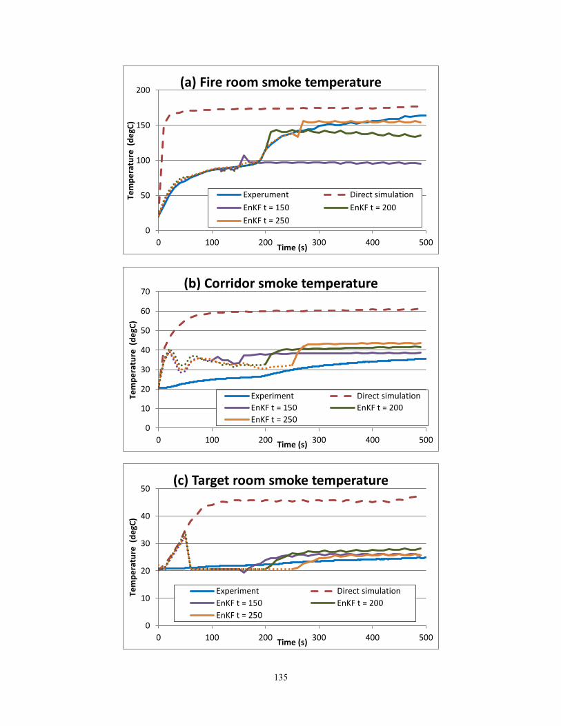
135

0

50

100

150

200

0 100 200 300 400 500

Tem

pe

ratu

re (

de

gC)

Time (s)

(a) Fire room smoke temperature

Experument Direct simulation

EnKF t = 150 EnKF t = 200

EnKF t = 250

0

10

20

30

40

50

60

70

0 100 200 300 400 500

Tem

pe

ratu

re (

de

gC)

Time (s)

(b) Corridor smoke temperature

Experiment Direct simulation

EnKF t = 150 EnKF t = 200

EnKF t = 250

0

10

20

30

40

50

0 100 200 300 400 500

Tem

pe

ratu

re (

de

gC)

Time (s)

(c) Target room smoke temperature

Experiment Direct simulation

EnKF t = 150 EnKF t = 200

EnKF t = 250

136

Fig 7.14 (a) to (f) Predictability of the EnKF model during a non-constant fire

0.0

0.1

0.2

0.3

0.4

0.5

0 100 200 300 400 500

Smo

ke la

yer

he

igh

t (m

)

Time (s)

(d) Fire room smoke layer height

Experiment Direct simulation

EnKF t = 150 EnKF t = 200

EnKF t = 250

0.0

0.1

0.2

0.3

0.4

0.5

0 100 200 300 400 500

Smo

ke la

yer

he

igh

t (m

)

Time (s)

(e) Corridor smoke layer height

Experiment Direct simulationEnKF t = 150 EnKF t = 200EnKF t = 250

0.0

0.1

0.2

0.3

0.4

0.5

0 100 200 300 400 500

Smo

ke la

yer

he

igh

t (m

)

Time (s)

(f) Target room smoke layer height

Experiment Direct simulation

EnKF t = 150 EnKF t = 200

EnKF t = 250

137

References

Hamill, Thomas M., Jeffrey S. Whitaker, and Chris Snyder. "Distance-dependent filtering of

background error covariance estimates in an ensemble Kalman filter." Monthly Weather

Review 129, no. 11 (2001): 2776-2790.

Melling, A. "Tracer particles and seeding for particle image velocimetry."Measurement Science

and Technology 8, no. 12 (1997): 1406.

138

Chapter 8 Conclusions and Future Work

8.1 Conclusions

This thesis outlined a general approach to forecasting building indoor environment by using

ensemble-based data assimilation algorithms. The results indicate that the proposed method can

improve predictability of a simple model by calibrating sensor measurements. Unlike other

methods that directly use measurement data as model inputs, the resulting models of this thesis

are able to statistically update model parameters to maintain the forecasting accuracy for longer

durations.

The models presented in this thesis provide noticeably accurate predictions and require low

computational resources compared to other conventional methods. The following is a list of

major findings and contributions from this thesis regarding using EnKF for indoor environment

forecasting:

▪This thesis research is among the very first studies of using numerical weather prediction

models and data assimilation techniques, specifically EnKF, for forecasting simulations of indoor

contaminant transport and building fire smoke spread. It is also one of the first times to achieve a

real-time forecasting of fire smoke spread in a scaled building model under a controlled

laboratory environment.

▪One of the most important parameters affecting the EnKF model’s performance is the number of

ensemble members. Unfortunately, there is still no theoretical principle for determining an

optimal number of ensemble members; it is usually determined by empirical methods such as

trial and error.

▪For the EnKF analysis, all sensor measurements are not necessarily provided at the same time

139

step. When the processing time of the simulation model is significantly shorter than the

observation time step, it is suggested that the system be arranged to obtain data in a sequential

order from each sensor rather than obtaining all measurements concurrently from all sensors.

▪When the method is applied to existing simulation models, filter divergence can be a potential

problem because the perturbation range is sometimes limited by the convergence criteria of the

simulation model. This can be mitigated by adding white noise to the simulation results to

increase the spread of ensemble members. In addition, modification of the simulation model is

sometimes necessary to enable perturbation of certain model parameters.

▪To achieve real-time forecasting, using localization methods to avoid spurious correlation,

instead of adding white noise, is suggested. This is because additional ensemble members must

compensate for the additional noises.

▪The EnKF is more flexible at applying different localization methods when certain model

parameters and model states are not highly correlated.

▪The convergence criteria of an implicit simulation model should be considered with the model

parameter perturbation range. When applying an explicit simulation model, the convergence

problem can be avoided, which means more freedom in parameter perturbation.

▪The range of parameter perturbation can be reasonably estimated using available measurements.

When the measurements are not directly obtainable, it can rely on other simulation tools with

higher accuracy (i.e., a CFD model).

▪The determination of measurement uncertainties should account for the assumptions of the

simulation model. For example, when a parameter is an average value of a physical condition,

the error of using one measurement to represent the mean should also be considered a

measurement uncertainty.

140

▪For noisy observations, such as the measurements obtained from the early stages of a

compartment fire, the EnKF analysis results are expected to deviate significantly from the

measurements. However, if the spread of ensemble perturbation is also very large, this may cause

the analysis results to fit too closely with the measurements, resulting in an imbalanced analysis,

which is considered suboptimal (Houtekamer and Mitchell 2005). To avoid this problem, the

observation uncertainty should also be increased.

8.2 Future works

8.2.1 Ensemble based DA algorithms for higher dimensional systems

In this thesis, the simulation models are all based on low dimensional systems wherein the

number of ensemble members is much greater than that of model nodes. Therefore, the number

of ensemble members is usually determined after the whole model structure has been outlined.

However, for a higher dimensional system, adding one ensemble member can significantly

increase the computational cost. Thus, the order in which the EnKF parameters are determined

becomes much more important in higher dimensional systems. For example, increasing the range

of parameter perturbation is necessary to avoid filter divergence but demands a higher number of

ensemble members, so the determination of optimal model parameters may require the testing of

different combinations of multiple parameters instead of optimizing one at each time.

8.2.2 Localization by modifying observation covariance

The localization method presented in this thesis is based on modifying simulation error

covariance. Chapter 7 introduces another method involving the modification of observation error

covariance. In general, localizing observations are considered more balanced than localizing

simulations, but they are also less accurate. The determination of the length scale is also different

141

(Greybush 2009). The major advantage of localizing observations is it can be applied to the local

transform ensemble Kalman filter (LETKF), while simulation localization cannot be

implemented. This may enable a comparison between EnKF and LETKF since the same

localization method is applied.

8.2.3 Other ensemble based DA algorithms

According to the literature reviews, each ensemble-based DA algorithm has its own advantages,

but there are very few ensemble-based DA studies related to building environment. In addition,

finding an ensemble-based DA method (and its corresponding model properties) that performs

better than other methods at solving a specific type of problem is still very challenging. The

study can only be conducted by direct comparisons of detailed models using different methods,

where each model is optimized independently, rather than using similar setups.

The following are some general suggestions for the selection of ensemble-based DA algorithms

to solve building environment problems:

▪DEnKF–It is more suitable for a system with noisy measurements but that uses a more accurate

simulation model. In this case, the magnitude of model state corrections in the analysis cycle can

be very small in order to avoid the filter divergence problem.

▪EnSRF–One of the most important characteristics of EnSRF is the non-uniqueness that different

ensembles can have the same covariance. This feature can be exploited to evaluate model

performance such as the computational and numerical properties of the filter (Tippett et al.

2002).

▪LETKF–For high dimensional systems with a low number of ensemble members, LETKF

requires a relatively large effective range for the localized box. This may significantly reduce the

efficiency of the system, so it is suggested for use with systems that have more measurements

142

available.

▪EnKF– The ensemble Kalman filter uses perturbed observation to maintain a reasonable range

of ensemble spread in order to avoid filter divergence. The EnKF is relatively more stable

compared to other methods but is sometimes considered suboptimal due to the additional

observation noises. However, when applied to high dimensional systems, its stability becomes

significant due to the lower number of ensemble members required.

8.2.4 Full-scale fire experiment

Although the results presented in Chapter 7 are showing the capability of EnKF in real-time

forecasting of compartment fire, the measurements are based on a scaled experiment under well-

controlled conditions in a laboratory. The temperature rise in the target room is relatively small

which makes it not easy to verify the model predictability. Therefore, a full scale fire experiment

is required to further study the effect of changing ventilation conditions as well as widen the

range of HRR change.

8.2.5 Reconstruction of a fire scene using available information

Reconstructions of fire scenes are generally performed in insurance and crime investigations. By

using information collected from the fire scene, such as a laboratory analysis report of on-site

fabric samples, investigators may be able to delineate the entire accident scene.

As several studies suggest (Shen 2008 and Chi 2011), these fire scene investigations can benefit

from computer simulations. CFD or zonal computer simulation models can help in the

reconstruction of a fire scene by establishing possible scenarios and identifying the most likely

case. However, the process can be very time consuming, as CFD simulations may take hours or

even days to process the results for one simple model. In such cases, ensemble-based DA

algorithms can first statistically outline the scene using simple zone models. Then, after

143

important parameters such as ignition source and HRR profile are determined, the information

can be applied to a CFD model to produce a more detailed fire scene reconstruction.

References

Greybush, Steven, Eugenia Kalnay, Takemasa Miyoshi, K. Ide, and B. Hunt. "EnKF localization

techniques and balance." In WMO 5th International Symposium on Data Assimilation.

Melbourne, Australia, pp. 6-9. 2009.

Shen, Tzu-Sheng, Yu-Hsiang Huang, and Shen-Wen Chien. "Using fire dynamic simulation

(FDS) to reconstruct an arson fire scene." Building and environment43, no. 6 (2008): 1036-1045.

Chi, Jen‐Hao, Sheng‐Hung Wu, and Chi‐Min Shu. "Using fire dynamics simulator to reconstruct

a hydroelectric power plant fire accident." Journal of forensic sciences 56, no. 6 (2011): 1639-

1644.

144

Appendix

145

Appendix Door Flow Rate Model

private static double[] doorflowRate(double doorH, double doorA, double roomHa, double roomHc, double Hda, double Hdc, double Pa, double Pc, double rhoa, double rhoc){ double mac = 0.0; double mca = 0.0; double mbd = 0.0; double mdb = 0.0; double g = 9.8; double rhoair = 1.20416; double cvent = 0.6; if (Hda>doorH){ //destination smoke layer height is always higher //smoke layer height (Hda) is above door soffit double dP1 = (Pa-Pc) - (rhoc-rhoa)*g*(roomHa-Hdc) - (rhoair-rhoa)*g*(Hdc-Hda); if (dP1 == 0){ mbd = 0.0; mdb = 0.0; }else{ mbd=Math.max(0.0,Math.abs(dP1)/dP1*flowRate(dP1,dP1,doorA,rhoa,cvent)); mdb=Math.max(0.0, -Math.abs(dP1)/dP1*flowRate(dP1,dP1,doorA,rhoa,cvent)); } }else if (Hdc>doorH){ // if smoke gets in destination room (Hda is below door soffit) // case 1, Hdc is above door soffit double dP1 = (Pa-Pc) - (rhoc-rhoa)*g*(roomHa-Hdc) - (rhoair-rhoa)*g*(Hdc-doorH); //deltaP at door soffit double dP2 = (Pa-Pc) - (rhoc-rhoa)*g*(roomHc-Hdc) - (rhoair-rhoa)*g*(Hdc-Hda); //deltaP at smoke layer Hda if (dP1>0){ // Normal Case if (dP2>0){ //Case B - 1 (No neutral layer) double Au = doorA/doorH*(doorH-Hda); double Ad = doorA/doorH*Hda; mac = flowRate(dP1,dP2,Au,rhoa,cvent); mbd = flowRate(dP2,dP2,Ad,rhoair,cvent); }else{ //Case C - 1 (Neutral layer exists) double Hna = Hdc-((Pa-Pc)-(roomHc-Hdc)*g*(rhoc-rhoa))/(rhoair-rhoa)/g; double Au = doorA/doorH*(doorH-Hna); double Ad1 = doorA/doorH*(Hna-Hda); double Ad2 = doorA/doorH*Hda; mac = flowRate(dP1,0,Au,rhoa,cvent); double mdb1 = flowRate(0,dP2,Ad1,rhoair,cvent); double mdb2 = flowRate(dP2,dP2,Ad2,rhoair,cvent); mdb = mdb1+mdb2; } } else { // Rare Case, dP1<0, back flow double Au = doorA/doorH*(doorH-Hda); double Ad = doorA/doorH*Hda; double mdb1 = flowRate(dP1,dP2,Au,rhoair,cvent); double mdb2 = flowRate(dP2,dP2,Ad,rhoair,cvent); mdb = mdb1 + mdb2; }

146

}else { // 2nd case, Hdc is below door soffit if (Hda<Hdc){ // Normally double dP1 = (Pa-Pc) - (rhoc-rhoa)*g*(roomHa-doorH); //at door soffit double dP2 = (Pa-Pc) - (rhoc-rhoa)*g*(roomHa-Hdc); //at Hdc double dP3 = (Pa-Pc) - (rhoc-rhoa)*g*(roomHa-Hdc) - (rhoair-rhoa)*g*(Hdc-Hda);//at Hda if (dP1>0){ // Normal Case if (dP2>0){ if (dP3>0){// Case B - 2 (No neutral layer) double Au1 = doorA/doorH*(doorH-Hdc); double Au2 = doorA/doorH*(Hdc-Hda); double Ad = doorA/doorH*Hda; double mac1 = flowRate(dP1,dP2,Au1,rhoa,cvent); double mac2 = flowRate(dP2,dP3,Au2,rhoa,cvent); mac = mac1 + mac2; mbd = flowRate(dP3,dP3,Ad,rhoair,cvent); } else {//Case C - 2 (Neutral layer is between Hda and Hdc) double Hna = Hdc-((Pa-Pc)-(roomHc-Hdc)*g*(rhoc-rhoa))/(rhoair-rhoa)/g; double Au1 = doorA/doorH*(doorH-Hdc); double Au2 = doorA/doorH*(Hdc-Hna); double Ad1 = doorA/doorH*(Hna-Hda); double Ad2 = doorA/doorH*Hda; double mac1 = flowRate(dP1,dP2,Au1,rhoa,cvent); double mac2 = flowRate(dP2,0,Au2,rhoa,cvent); double mdb1 = flowRate(0,dP3,Ad1,rhoair,cvent); double mdb2 = flowRate(dP3,dP3,Ad2,rhoair,cvent); mac = mac1 + mac2; mdb = mdb1 + mdb2; } }else{ // dP2 < 0, Case C - 3 (Neutral layer is between door soffit and Hdc) double Hna = Hdc-((Pa-Pc)-(roomHc-Hdc)*g*(rhoc-rhoa))/(rhoair-rhoa)/g; double Au = doorA/doorH*(doorH-Hna); double Ad1 = doorA/doorH*(Hna-Hdc); double Ad2 = doorA/doorH*(Hdc-Hda); double Ad3 = doorA/doorH*Hda; mac = flowRate(dP1,0,Au,rhoa,cvent); mca = flowRate(0,dP2,Ad1,rhoc,cvent); double mdb1 = flowRate(dP2,dP3,Ad2,rhoair,cvent); double mdb2 = flowRate(dP3,dP3,Ad3,rhoair,cvent); mdb = mdb1 + mdb2; } }else{ // Rare Case, dP1<0, back flow double Au1 = doorA/doorH*(doorH-Hdc); double Au2 = doorA/doorH*(Hdc-Hda); double Ad = doorA/doorH*Hda; mca = flowRate(dP1,dP2,Au1,rhoa,cvent); double mdb1 = flowRate(dP2,dP3,Au2,rhoa,cvent); double mdb2 = flowRate(dP3,dP3,Ad,rhoair,cvent); mdb = mdb1 + mdb2; } }else { // For far away room, long simulation

147

double dP1 = (Pa-Pc) - (rhoc-rhoa)*g*(roomHa-doorH); //at door soffit double dP2 = (Pa-Pc) - (rhoc-rhoa)*g*(roomHa-Hda); //at Hda double dP3 = (Pa-Pc) - (rhoc-rhoa)*g*(roomHa-Hda) - (rhoc-rhoair)*g*(Hda-Hdc);//at Hdc if (dP1>0){ // Normal Case if (dP2>0){ if (dP3>0){// Case B - 2 (No neutral layer) double Au = doorA/doorH*(doorH-Hda); double Ad1 = doorA/doorH*(Hda-Hdc); double Ad2 = doorA/doorH*Hdc; double mbd1 = flowRate(dP2,dP3,Ad1,rhoair,cvent); double mbd2 = flowRate(dP3,dP3,Ad2,rhoair,cvent); mac = flowRate(dP1,dP2,Au,rhoa,cvent); mbd = mbd1+mbd2; } else {//Case C - 2 (Neutral layer is between Hda and Hdc) double Hna = Hda - (Pa-Pc)/(rhoc-rhoair)/g+(rhoc-rhoa)/(rhoc-rhoair)*Hda; double Au1 = doorA/doorH*(doorH-Hda); double Au2 = doorA/doorH*(Hda-Hna); double Ad1 = doorA/doorH*(Hna-Hdc); double Ad2 = doorA/doorH*Hdc; double mac1 = flowRate(dP1,dP2,Au1,rhoa,cvent); double mac2 = flowRate(dP2,0,Au2,rhoair,cvent); double mdb1 = flowRate(0,dP3,Ad1,rhoc,cvent); double mdb2 = flowRate(dP3,dP3,Ad2,rhoair,cvent); mac = mac1+mac2; mdb = mdb1+mdb2; } }else{ // dP2 < 0, Case C - 3 (Neutral layer is between door soffit and Hdc) double Hna = roomHa - (Pa - Pc)/g/(rhoc - rhoa); double Au = doorA/doorH*(doorH-Hna); double Ad1 = doorA/doorH*(Hna-Hda); double Ad2 = doorA/doorH*(Hda-Hdc); double Ad3 = doorA/doorH*Hdc; mac = flowRate(dP1,0,Au,rhoa,cvent); double mdb1 = flowRate(0,dP2,Ad1,rhoc,cvent); double mdb2 = flowRate(dP2,dP3,Ad2,rhoair,cvent); double mdb3 = flowRate(dP3,dP3,Ad3,rhoair,cvent); mdb = mdb1 + mdb2 +mdb3; } }else{ // Rare Case, dP1<0, back flow double Au1 = doorA/doorH*(doorH-Hda); double Au2 = doorA/doorH*(Hda-Hdc); double Ad = doorA/doorH*Hdc; double mca1 = flowRate(dP1,dP2,Au1,rhoc,cvent); double mca2 = flowRate(dP2,dP3,Au2,rhoc,cvent); mca = mca1 + mca2; mdb = flowRate(dP3,dP3,Ad,rhoair,cvent); } } }