14 Global glacier changes: facts and figures 15

Box 3.2 ASTER satellite images

Satellite data are an important resource for global-scale glacier monitoring. They enable the observation of land ice masses over large spatial scales using a globally uniform set of data and methods, and independent of monitoring obstacles on the ground such as access problems and financial limitations on institutional levels. On the other hand, space-aided glacier moni-toring relies on a small number of space agencies, the financial resources and political willingness of which are thus crucial for the maintenance of the monitoring system. Typical glaciological parameters that can be observed from space are glacier areas and their changes over time, snow lines, glacier topography and glacier thickness changes, and glacier flow and its changes over time (Kääb 2005).

The satellite images in this publication were taken by the US/Japan Advanced Thermal Emission and Reflection Radiometer (ASTER) onboard the NASA Terra spacecraft. They were acquired within the Global Land Ice Measurements from Space (GLIMS) initiative and obtained through the US Geological Survey/NASA EOS data gateway. The ASTER sensor includes two spectral bands in the visible range (green and red), one band in the near-infrared, six bands in the short-wave infrared, and five bands in the thermal infrared. The most important bands for glaciological applications are the visible, near- and short-wave infrared bands (Fig. 3.1 a–d). They allow for automatic mapping of ice and snow areas. This technique exploits the large difference in ice and snow reflectivity between the visible, near- and short-wave infrared spectrum, and enables the fast compilation of a large number of glacier outlines and their changes over time. In addition to the above-mentioned nadir bands, ASTER has also a back-looking stereo sensor that, together with the corresponding nadir image, allows for the photogrammetric computation of glacier topography and its changes over time (Kääb 2005).

Global distribution of glaciers and ice caps

The need for a worldwide inventory of existing per-ennial ice and snow masses was first considered dur-ing the International Hydrological Decade declared by UNESCO for the period of 1965–1974 (Hoelzle and Trindler 1998, UNESCO 1970). The Temporal Technical Secretariat for the World Glacier Inventory (TTS/WGI) was established in 1975 to prepare guidelines for the compilation of such an inventory and to collect available data sets from different countries (WGMS 1989). These tasks were continued by its successor organisation, the WGMS, after 1986. In 1989, a status report on the WGI was published including detailed information on about 67 000 glaciers covering some 180 000 km2 and pre-liminary estimates for the other glacierised regions, both based on aerial photographs, maps, and satellite images (WGMS 1989). The detailed inventory includes tabular information about geographic location, area, length, orientation, elevation and classification of mor-phological type (a selection of different types is shown in Figures 3.2–3.5, and more in the other chapters) and moraines, which are related to the geographical coordi-nates of glacier label points. Due to the different data sources, the entries of the WGI do not refer to one spe-cific year but can be viewed as a snapshot of the glacier distribution around the 1960s. The average map year is 1964 with a standard deviation of eleven years, and a time range from 1901 to 1993. In 1998, the WGMS

and the NSIDC agreed to work together, pooled their data sources and made the inventory available online in 1999 via the NSIDC website (Box 3.1). Since then, several plausibility checks, subsequent data corrections and updates of the inventory have been carried out, including updates and new data sets from the former Soviet Union and China. At present the database con-tains information for over 100 000 glaciers throughout the world with an overall area of about 240 000 km2 (NSIDC 2008). This corresponds to about half of the to-tal number and roughly one-third of the global ice cover of glaciers and ice caps, which are estimated at 160 000 and 685 000 km2, respectively, by Dyurgerov and Meier (2005) based mainly on the WGI (WGMS 1989) and ad-ditional estimates from the literature.

In 1995, the GLIMS initiative was launched, in close col-laboration with the NSIDC and the WGMS, to continue the inventorying task with space-borne sensors as a logical extension of the WGI and storing the full complement of the WGMS-defined glacier characteristics (see Kääb et al. 2002, Bishop et al. 2004, Kargel et al. 2005). GLIMS is designed to monitor the world’s glaciers primarily us-ing data from optical satellite instruments, such as the Advanced Spaceborne Thermal Emission and reflection Radiometer (ASTER), an instrument that is required on board of Terra satellite (Box 3.2). A geographic infor-

A first attempt to compile a world glacier inventory started in the 1970s based mainly on aerial photographs and maps. Up to now, it resulted in a detailed inventory of more than 100 000 glaciers covering an area of about 240 000 km2, and in preliminary estimates for the remaining ice cover of some 445 000 km2. Today the task of inventorying glaciers worldwide is continued for the most part based on satellite images.

Global distribution of glaciers and ice caps 3

Fig. 3.1 a—d Glaciers in Bhutan, Himalayas (57x42 km): a) green ASTER band, b) shortwave-infrared, c) colour composite of the green, red and near-infrared bands, and d) colour composite of red, near-infrared and short-wave infrared bands.

Box 3.1 Online data access to the WGI and GLIMS databases

The World Glacier Inventory (WGI) currently has detailed information on over 100 000 glaciers throughout the world. Pa-rameters within the inventory include coordinates (latitude and longitude) per glacier, together with tabular information about geographic location, area, length, orientation and elevation, as well as classifications of morphological type and moraines. The entire database can be searched by entering attributes and geographical location. The data sets thus selected or the entire database can be downloaded via the websites of the NSIDC, the WGMS, or of the GLIMS glacier database.

The GLIMS Glacier Database stores some 62 000 digital glacier outlines together with tabular information such as glacier area, length and elevation. The database can be queried using a text or mapping search interface. Glacier outlines with the related information can be downloaded from the GLIMS website in several formats used by geographic information system software products.

WGI at NSIDC: http://nsidc.org/data/glacier_inventory/index.htmlWGI at WGMS: http://www.wgms.ch/wgi.htmlGLIMS Glacier Database: http://glims.colorado.edu/glacierdata/

Fig. 3.1a

Fig. 3.1c Fig. 3.1d

Fig. 3.1b

16 Global glacier changes: facts and figures 17

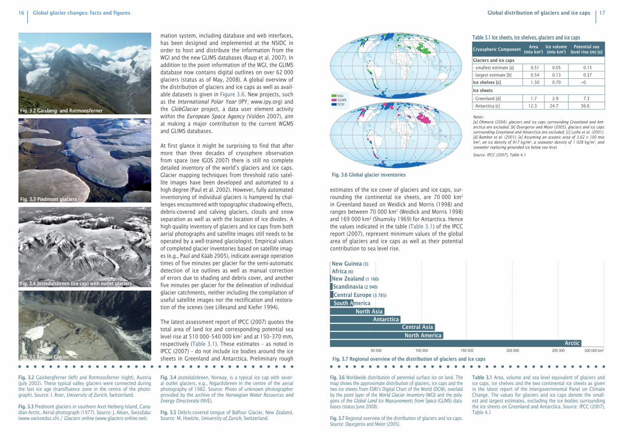
50 000 100 000 150 000 200 000 250 000 300 000 km2

New Guinea (3)

Africa (6)

New Zealand (1 160)

Central Europe (3 785)

South America

North Asia Antarctica

Central Asia

North AmericaArctic

Scandinavia (2 940)

estimates of the ice cover of glaciers and ice caps, sur-rounding the continental ice sheets, are 70 000 km2 in Greenland based on Weidick and Morris (1998) and ranges between 70 000 km2 (Weidick and Morris 1998) and 169 000 km2 (Shumsky 1969) for Antarctica. Hence the values indicated in the table (Table 3.1) of the IPCC report (2007), represent minimum values of the global area of glaciers and ice caps as well as their potential contribution to sea level rise.

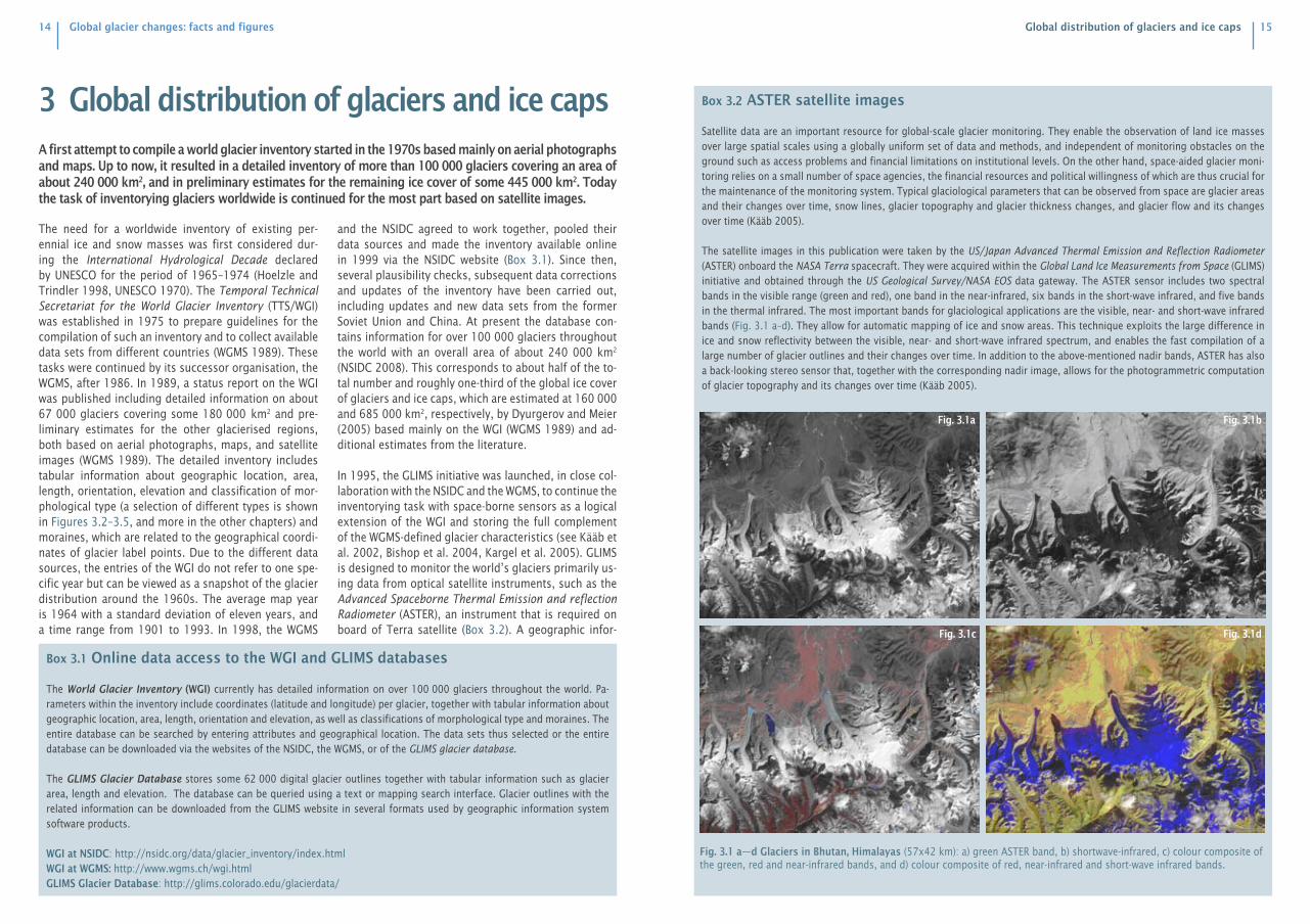
mation system, including database and web interfaces, has been designed and implemented at the NSIDC in order to host and distribute the information from the WGI and the new GLIMS databases (Raup et al. 2007). In addition to the point information of the WGI, the GLIMS database now contains digital outlines on over 62 000 glaciers (status as of May, 2008). A global overview of the distribution of glaciers and ice caps as well as avail-able datasets is given in Figure 3.6. New projects, such as the International Polar Year (IPY; www.ipy.org) and the GlobGlacier project, a data user element activity within the European Space Agency (Volden 2007), aim at making a major contribution to the current WGMS and GLIMS databases.

At first glance it might be surprising to find that after more than three decades of cryosphere observation from space (see IGOS 2007) there is still no complete detailed inventory of the world’s glaciers and ice caps. Glacier mapping techniques from threshold ratio satel-lite images have been developed and automated to a high degree (Paul et al. 2002). However, fully automated inventorying of individual glaciers is hampered by chal-lenges encountered with topographic shadowing effects, debris-covered and calving glaciers, clouds and snow separation as well as with the location of ice divides. A high quality inventory of glaciers and ice caps from both aerial photographs and satellite images still needs to be operated by a well-trained glaciologist. Empirical values of completed glacier inventories based on satellite imag-es (e.g., Paul and Kääb 2005), indicate average operation times of five minutes per glacier for the semi-automatic detection of ice outlines as well as manual correction of errors due to shading and debris cover, and another five minutes per glacier for the delineation of individual glacier catchments, neither including the compilation of useful satellite images nor the rectification and restora-tion of the scenes (see Lillesand and Kiefer 1994).

The latest assessment report of IPCC (2007) quotes the total area of land ice and corresponding potential sea level rise at 510 000–540 000 km2 and at 150–370 mm, respectively (Table 3.1). These estimates – as noted in IPCC (2007) – do not include ice bodies around the ice sheets in Greenland and Antarctica. Preliminary rough

Fig. 3.2 Gaisbergferner (left) and Rotmoosferner (right), Austria (July 2002). These typical valley glaciers were connected during the last ice age (transfluence zone in the centre of the photo-graph). Source: I. Roer, University of Zurich, Switzerland.

Fig. 3.3 Piedmont glaciers in southern Axel Heiberg Island, Cana-dian Arctic. Aerial photograph (1977). Source: J. Alean, SwissEduc (www.swisseduc.ch) / Glaciers online (www.glaciers-online.net).

Fig. 3.4 Jostedalsbreen, Norway, is a typical ice cap with sever-al outlet glaciers, e.g., Nigardsbreen in the centre of the aerial photography of 1982. Source: Photo of unknown photographer provided by the archive of the Norwegian Water Resources and Energy Directorate (NVE).

Fig. 3.5 Debris-covered tongue of Balfour Glacier, New Zealand. Source: M. Hoelzle, University of Zurich, Switzerland.

Global distribution of glaciers and ice caps

Fig. 3.2 Gaisberg- and Rotmoosferner

Fig. 3.3 Piedmont glaciers

Fig. 3.4 Jostedalsbreen (ice cap) with outlet glaciers

Fig. 3.5 Balfour Glacier

Fig. 3.6 Worldwide distribution of perennial surface ice on land. The map shows the approximate distribution of glaciers, ice caps and the two ice sheets from ESRI’s Digital Chart of the World (DCW), overlaid by the point layer of the World Glacier Inventory (WGI) and the poly-gons of the Global Land Ice Measurements from Space (GLIMS) data-bases (status June 2008).

Fig. 3.7 Regional overview of the distribution of glaciers and ice caps. Source: Dyurgerov and Meier (2005).

Table 3.1 Area, volume and sea level equivalent of glaciers and ice caps, ice shelves and the two continental ice sheets as given in the latest report of the Intergovernmental Panel on Climate Change. The values for glaciers and ice caps denote the small-est and largest estimates, excluding the ice bodies surrounding the ice sheets on Greenland and Antarctica. Source: IPCC (2007), Table 4.1

Fig. 3.6 Global glacier inventories

GLIMS WGI

DCW

Fig. 3.7 Regional overview of the distribution of glaciers and ice caps

Table 3.1 Ice sheets, ice shelves, glaciers and ice caps

Cryospheric ComponentArea

(mio km2)Ice volume (mio km3)

Potential sea level rise (m) [e]

Glaciers and ice caps

- smallest estimate [a] 0.51 0.05 0.15

- largest estimate [b] 0.54 0.13 0.37

Ice shelves [c] 1.50 0.70 ~0

Ice sheets

- Greenland [d] 1.7 2.9 7.3

- Antarctica [c] 12.3 24.7 56.6

Notes:[a] Ohmura (2004); glaciers and ice caps surrounding Greenland and Ant-arctica are excluded; [b] Dyurgerov and Meier (2005); glaciers and ice caps surrounding Greenland and Antarctica are excluded; [c] Lythe et al. (2001); [d] Bamber et al. (2001); [e] Assuming an oceanic area of 3.62 × 100 mio km2, an ice density of 917 kg/m3, a seawater density of 1 028 kg/m3, and seawater replacing grounded ice below sea level.

Source: IPCC (2007), Table 4.1