Geophysicae Application of model-based spectral … · Geophysicae Application of model-based spectral analysis to wind-proﬁler radar observations ... (Oppenheim and Shafer, 1989;

Annales Geophysicae (2001) 19: 815–824c© European Geophysical Society 2001Annales

Geophysicae

Application of model-based spectral analysis to wind-profiler radarobservations

E. Boyer1, M. Petitdidier 2, W. Corneil2, C. Adnet3, and P. Larzabal1,4

1LESiR/ENS Cachan, UPRESA 8029, 61 avenue du president Wilson, 94235 Cachan cedex, France2CETP, 10-12 Avenue de l’Europe, 78140 Velizy, France3THALES Air Dfense, 7-9 rue des Mathurins, Bagneux France4IUT de Cachan, CRIIP, Universite Paris Sud, 9 avenue de la division Leclerc, 94 234 Cachan cedex, France

Received: 24 July 2000 – Revised: 13 February 2001 – Accepted: 5 March 2001

Abstract. A classical way to reduce a radar’s data is to com-pute the spectrum using FFT and then to identify the differ-ent peak contributions. But in case an overlapping betweenthe different echoes (atmospheric echo, clutter, hydrometeorecho. . . ) exists, Fourier-like techniques provide poor fre-quency resolution and then sophisticated peak-identificationmay not be able to detect the different echoes. In order toimprove the number of reduced data and their quality rel-ative to Fourier spectrum analysis, three different methodsare presented in this paper and applied to actual data. Theirapproach consists of predicting the main frequency-compo-nents, which avoids the development of very sophisticatedpeak-identification algorithms. The first method is based oncepstrum properties generally used to determine the shift be-tween two close identical echoes. We will see in this pa-per that this method cannot provide a better estimate thanFourier-like techniques in an operational use. The secondmethod consists of an autoregressive estimation of the spec-trum. Since the tests were promising, this method was ap-plied to reduce the radar data obtained during two thunder-storms. The autoregressive method, which is very simple toimplement, improved the Doppler-frequency data reductionrelative to the FFT spectrum analysis. The third method ex-ploits a MUSIC algorithm, one of the numerous subspace-based methods, which is well adapted to estimate spectracomposed of pure lines. A statistical study of performancesof this method is presented, and points out the very goodresolution of this estimator in comparison with Fourier-liketechniques. Application to actual data confirms the goodqualities of this estimator for reducing radar’s data.

Key words. Meteorology and atmospheric dynamics (trop-ical meteorology)- Radio science (signal processing)- Gen-eral (techniques applicable in three or more fields)

Correspondence to:E. Boyer ([email protected])

1 Introduction

Wind-profiler radars generally operate in the VHF and UHFbands, and are used to observe the scattering of radiowavesfrom clear-air refractive-index fluctuations. Although notnecessarily optimised for detecting other types of scatter-ers, the signals that the radars receive, nevertheless, containnon-clear air echoes, such as hydrometeors at UHF, light-ning emissions at VHF, clutter at UHF and VHF, etc. Asthese radars become an operational tool for short-term pre-diction and forecasting, as well as a research instrument forboundary-layer tropospheric and stratospheric studies, thenrobust algorithms have to be implemented in order to deter-mine the different Doppler frequencies present in the signal,to classify and select the important ones, and to compute thewind. Primarily, the ordinary algorithm used contains thefollowing steps: coherent integrations of the signal, applica-tion of a window, computation of the spectrum using FFTand incoherent integrations (Tsuda, 1989). Sato and Wood-man (1982) computed the autocorrelation function instead ofthe FFT. Many approaches have been developed to search theechoes and to extract the corresponding Doppler frequencies(Yamamoto et al., 1988; Hocking, 1997) with the selection ofthe right frequency as the final step in order to compute thewind velocity. When the sought echo is unique and well sep-arated from the clutter, and located at 0 Hz, any algorithmworks, yet the fastest is the best. But over a whole verti-cal wind-profile (i.e. wind as a function of the altitude at agiven time) and in all weather conditions, this is not the case.Several echoes which may overlap could be present in thespectrum. The classical case of overlapping is the one be-tween clutter and atmospheric echo. Fourier-like techniquesprovide poor results for close echoes; the frequency reso-lution is not enough to separate the different contributions.The atmospheric echo may be approximated by a Gaussianshape, but the clutter does not correspond to any analyticalmodel, except when it may be considered as a single spectral

816 E. Boyer et al.: Application of model-based spectral analysis to wind-profiler radar observations

FIGURES

-0.5 -0.4 -0.3 -0.2 -0.1 0 0.1 0.2 0.3 0.4 0.50

200

400

600

800

1000

1200

-0.5 -0.4 -0.3 -0.2 -0.1 0 0.1 0.2 0.3 0.4 0.50

200

400

600

800

1000

1200

CEPSTRUM OF THE SIGNAL : ( )CE S f* ( )

SPECTRUM OF THE SIGNAL

Fig.1 Cepstrum results

Normalized frequency

Fig.1.b

CEPSTRUM OF THE PERIODICAL TERM

( )CE f f fδ δ( ) ( )+ − 0


Fig.1.d

Fig.2 Application of the cepstrum algorithm to two

different Gaussian echoes

CEPSTRUM OF THE SIGNAL SPECTRUM OF THE SIGNAL


Fig.2.a


Fig.2.b

-0.5 -0.4 -0.3 -0.2 -0.1 0 0.1 0.2 0.3 0.4 0.50

2

4

6

8

10

12

14

16

18

20

( )CE S f( )


Fig.1.c


Fig.1.a

-0.5 -0.4 -0.3 -0.2 -0.1 0 0.1 0.2 0.3 0.4 0.5 0

50

100

150

200

250

powe

r

powe

r

powe

r

powe

r

-0.5 -0.4 -0.3 -0.2 -0.1 0 0.1 0.2 0.3 0.4 0.5-5

0

5

10

15

20

25

30

35

40

powe

r (dB

)

-0.5 -0.4 -0.3 -0.2 -0.1 0 0.1 0.2 0.3 0.4 0.50

20

40

60

80

100

120

140

powe

r (dB

)

(a) (b)

FIGURES

-0.5 -0.4 -0.3 -0.2 -0.1 0 0.1 0.2 0.3 0.4 0.50

200

400

600

800

1000

1200

-0.5 -0.4 -0.3 -0.2 -0.1 0 0.1 0.2 0.3 0.4 0.50

200

400

600

800

1000

1200





Fig.1.b


( )CE f f fδ δ( ) ( )+ − 0


Fig.1.d





Fig.2.a


Fig.2.b

-0.5 -0.4 -0.3 -0.2 -0.1 0 0.1 0.2 0.3 0.4 0.50

2

4

6

8

10

12

14

16

18

20

( )CE S f( )


Fig.1.c


Fig.1.a

-0.5 -0.4 -0.3 -0.2 -0.1 0 0.1 0.2 0.3 0.4 0.5 0

50

100

150

200

250

powe

r

powe

r

powe

r

powe

r

-0.5 -0.4 -0.3 -0.2 -0.1 0 0.1 0.2 0.3 0.4 0.5-5

0

5

10

15

20

25

30

35

40

powe

r (dB

)

-0.5 -0.4 -0.3 -0.2 -0.1 0 0.1 0.2 0.3 0.4 0.50

20

40

60

80

100

120

140

powe

r (dB

)

(c) (d)

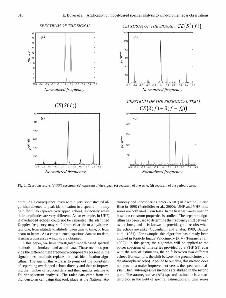
Fig. 1. Cepstrum results(a) FFT spectrum,(b) cepstrum of the signal,(c) cepstrum of one echo,(d) cepstrum of the periodic term.

point. As a consequence, even with a very sophisticated al-gorithm devoted to peak identification in a spectrum, it maybe difficult to separate overlapped echoes, especially whentheir amplitudes are very different. As an example, in UHF,if overlapped echoes could not be separated, the identifiedDoppler frequency may shift from clear-air to a hydrome-teor one, from altitude to altitude, from time to time, or frombeam to beam. As a consequence, spurious data or no data,if using a consensus window, are obtained.

In this paper, we have investigated model-based spectralmethods on simulated and actual data. These methods pro-vide the different main frequency-components present in thesignal; these methods replace the peak-identification algo-rithm. The aim of this work is to point out the possibilityof separating overlapped echoes directly and then to improv-ing the number of reduced data and their quality relative toFourier spectrum analysis. The radar data came from thethunderstorm campaign that took place at the National As-

tronomy and Ionospheric Center (NAIC) in Arecibo, PuertoRico in 1998 (Petitdidier et al., 2000); UHF and VHF timeseries are both used in our tests. In the first part, an estimationbased on cepstrum properties is studied. The cepstrum algo-rithm has been used to determine the frequency shift betweentwo echoes, and it is known to provide good results whenthe echoes are alike (Oppenheim and Shafer, 1989; Balluetet al., 1981). For example, this algorithm has already beenapplied in Particle Image Velocimetry (PIV) (Fournel et al.,1992). In this paper, the algorithm will be applied to thepower spectrum of time series provided by a VHF ST radarwith the aim of estimating the shift between two differentechoes (for example, the shift between the ground clutter andthe atmospheric echo). Applied to our data, this method doesnot provide a major improvement versus the spectrum anal-ysis. Then, autoregressive methods are studied in the secondpart. The autoregressive (AR) spectral estimator is a stan-dard tool in the field of spectral estimation and time series

E. Boyer et al.: Application of model-based spectral analysis to wind-profiler radar observations 817

FIGURES

-0.5 -0.4 -0.3 -0.2 -0.1 0 0.1 0.2 0.3 0.4 0.50

200

400

600

800

1000

1200

-0.5 -0.4 -0.3 -0.2 -0.1 0 0.1 0.2 0.3 0.4 0.50

200

400

600

800

1000

1200





Fig.1.b


( )CE f f fδ δ( ) ( )+ − 0


Fig.1.d





Fig.2.a


Fig.2.b

-0.5 -0.4 -0.3 -0.2 -0.1 0 0.1 0.2 0.3 0.4 0.50

2

4

6

8

10

12

14

16

18

20

( )CE S f( )


Fig.1.c


Fig.1.a

-0.5 -0.4 -0.3 -0.2 -0.1 0 0.1 0.2 0.3 0.4 0.5 0

50

100

150

200

250

powe

r

powe

r

powe

r

powe

r

-0.5 -0.4 -0.3 -0.2 -0.1 0 0.1 0.2 0.3 0.4 0.5-5

0

5

10

15

20

25

30

35

40

powe

r (dB

)

-0.5 -0.4 -0.3 -0.2 -0.1 0 0.1 0.2 0.3 0.4 0.50

20

40

60

80

100

120

140

powe

r (dB

)

Fig. 2. Application of the cepstrum algorithm on two different Gaussian echoes.

analysis (Kay and Marple, 1981). This method is applied di-rectly to time series. Subspace-based methods are presentedin the third part. The key idea consists in a decompositionof the observation space in two subspaces: the signal sub-space containing the echoes, and the noise subspace (Bienv-enue and Kopp, 1979, Schmidt, 1986). This decompositionis realized by computing the covariance matrix of the signal,which is then decomposed into its eigenvectors. The signifi-cant eigenvalues correspond to signal subspace eigenvectorsand the other eigenvalues correspond to the noise subspace.

2 Exploitation of the power cepstrum

2.1 The power cepstrum algorithm

In the cepstrum algorithm, the power spectrumS∗(f ) issupposed to be the sum of two identical echoes,f0 shifted(Fig. 1a):

S∗(f ) = S(f ) + S(f − f0) (1)

s∗(t) = s(t)(1 + e2jπf0t ) (2)

wheres(t) is the Fourier transform ofS(f ) ands∗(t) is theFourier transform ofS∗(f ). Let us define the complex loga-rithm by

ln c(S) = ln |S| + i arg(S) (3)

where arg(S) represents the unwrapped phase ofS to ensurethe uniqueness of the function. In the development

ln c(s∗(t)

)= ln c

(s(t)

)+ ln c

(1 + e2jπf0t

)(4)

the term lnc(1 + e2jπf0t

)is af0 periodical: a Fourier trans-

form of Eq. (4) exhibits a peak at the expected frequency,f0.Consequently, the power cepstrum ofS∗(f ) is defined by:

CE(S∗(f )

)=

∣∣∣∣FT(

ln c[FT

(S∗(f )

)])∣∣∣∣

=

∣∣∣∣FT(

ln c[s∗(t)

])∣∣∣∣ (5)

whereCE denotes the cepstrum operator andFT the FourierTransform operator. (5) can be rewritten as

CE(S∗(f )

)= CE

(S(f )

)+ CE

(δ(f ) + δ(f − f0)

)(6)

whereδ(f ) denotes the Dirac distribution.The cepstrum operator is generally applied directly on a

time series, but in our case, the cepstrum operator is appliedon spectra because we estimate the shift between two Gaus-sian spectra. Consequently, cepstra are represented with a“frequency” axis in Fig. 1 (b, c and d).

The second term

CE(δ(f ) + δ(f − f0)

)= FT

(ln c

[1 + e2jπf0t

])of Eq. (6), represented in Fig. 1d, exhibits a peak at thef0frequency and harmonics which are easily interpreted by theTaylor expansion of the logarithm function. In Fig. 1b, wecan easily detect this peak but in some cases, the first termCE

(S(f )

)+ (represented in Fig. 1c) can hide that peak and

the estimation won’t be possible (especially when the secondGaussian echo presents a significant attenuation in compari-son with the first one).

2.2 Simulation results

For simulations, the spectrum of the signal has been com-puted as proposed by Papoulis (1965):

S∗(f ) =1

Ninc

Ninc∑m=1

(Sth(f ) + σ 2

b

)∣∣ym

∣∣2 (7)

whereSth(f ) is the theoretical spectrum,σ 2b is an additive

noise power,Ninc is the number of incoherent integration andym is a Gaussian random variable with unit standard devia-tion. We took 256 points for the FFT algorithm.


Fig.3

AR method : test on the number of pole

normalized frequency normalized frequency

normalized frequency normalized frequency

pow

er (

dB)

(a) Experimental spectrum

(b) p=12

(c) p=5

(d) p=50

103

102

101

100

10-1

10-2

-0.6 0.6 -0.2 0 0.2 -0.6 0.6 -0.2 0 0.2

pow

er (

dB)

pow

er (

dB)

pow

er (

dB)

-0.6 0.6 -0.2 0 0.2 -0.8 1 -0.2 0 0.2

102

101

100

10-1

102

101

100

10-1

30

20

10

0

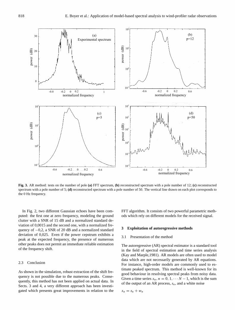
Fig. 3. AR method: tests on the number of pole(a) FFT spectrum,(b) reconstructed spectrum with a pole number of 12;(c) reconstructedspectrum with a pole number of 5;(d) reconstructed spectrum with a pole number of 50. The vertical line drawn on each plot corresponds tothe 0 Hz frequency.

In Fig. 2, two different Gaussian echoes have been com-puted: the first one at zero frequency, modeling the groundclutter with a SNR of 15 dB and a normalized standard de-viation of 0,0015 and the second one, with a normalized fre-quency of−0,2, a SNR of 20 dB and a normalized standarddeviation of 0,025. Even if the power cepstrum exhibits apeak at the expected frequency, the presence of numerousother peaks does not permit an immediate reliable estimationof the frequency shift.

2.3 Conclusion

As shown in the simulation, robust extraction of the shift fre-quency is not possible due to the numerous peaks. Conse-quently, this method has not been applied on actual data. InSects. 3 and 4, a very different approach has been investi-gated which presents great improvements in relation to the

FFT algorithm. It consists of two powerful parametric meth-ods which rely on different models for the received signal.

3 Exploitation of autoregressive methods

3.1 Presentation of the method

The autoregressive (AR) spectral estimator is a standard toolin the field of spectral estimation and time series analysis(Kay and Marple,1981). AR models are often used to modeldata which are not necessarily generated by AR equations.For instance, high-order models are commonly used to es-timate peaked spectrum. This method is well-known for itsgood behaviour in resolving spectral peaks from noisy data.Given a time seriesxn, n = 0, 1, · · ·N − 1, which is the sumof the output of an AR process,sn, and a white noise

xn = sn + wn


5 10 15 20 25 30 35 40 45 500.024

0.026

0.028

0.03

0.032

0.034

0.036

0.038

5 10 15 20 25 30 35 40 45 50-0.035

-0.03

-0.025

-0.02

-0.015

-0.01

-0.005

0 5 10 15 20 25 30 35 40 45 500.7

0.75

0.8

0.85

0.9

0.95

1

-0.5 -0.4 -0.3 -0.2 -0.1 0 0.1 0.2 0.3 0.4 0.5-5

0

5

10

15

20

25

30

35

Fig.4.c

Fig.4.b

Fig.4.d

Fig.4.a p

p p

normalized frequency

pow

er (

dB)

F C

mea

n rm

s

Fig.4 AR method: choice of the order p: two Gaussian echoes with f1=0.1 σ1=0.04

SNR1=20 dB ; f2=0.21 σ2=0.005 SNR2=18 dB.

mea

n bi

as

(a) (b)

5 10 15 20 25 30 35 40 45 500.024

0.026

0.028

0.03

0.032

0.034

0.036

0.038

5 10 15 20 25 30 35 40 45 50-0.035

-0.03

-0.025

-0.02

-0.015

-0.01

-0.005

0 5 10 15 20 25 30 35 40 45 500.7

0.75

0.8

0.85

0.9

0.95

1

-0.5 -0.4 -0.3 -0.2 -0.1 0 0.1 0.2 0.3 0.4 0.5-5

0

5

10

15

20

25

30

35

Fig.4.c

Fig.4.b

Fig.4.d

Fig.4.a p

p p


pow

er (

dB)

F C

mea

n rm

s


SNR1=20 dB ; f2=0.21 σ2=0.005 SNR2=18 dB.

mea

n bi

as

(c) (d)

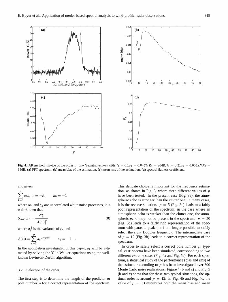
Fig. 4. AR method: choice of the orderp: two Gaussian echoes withf1 = 0.1σ1 = 0.04SNR1 = 20dB;f2 = 0.21σ2 = 0.005SNR2 =

18dB. (a) FFT spectrum,(b) mean bias of the estimation,(c) mean rms of the estimation,(d) spectral flatness coefficient.

and givenp∑

k=0

aksn−k = −ξn a0 = −1

wherewn andξn are uncorrelated white noise processes, it iswell-known that

SAR(ω) =σ 2

ξ∣∣A(ω)∣∣2 (8)

whereσ 2ξ is the variance ofξn and

A(ω) =

p∑k=0

ake−jωk a0 = −1 .

In the application investigated in this paper,ak will be esti-mated by solving the Yule-Walker equations using the well-known Levinson-Durbin algorithm.

3.2 Selection of the order

The first step is to determine the length of the predictor orpole numberp for a correct representation of the spectrum.

This delicate choice is important for the frequency estima-tion, as shown in Fig. 3, where three different values ofp

have been tested. In the present case (Fig. 3a), the atmo-spheric echo is stronger than the clutter one; in many cases,it is the reverse situation.p = 5 (Fig. 3c) leads to a fairlypoor representation of the spectrum; in the case where anatmospheric echo is weaker than the clutter one, the atmo-spheric echo may not be present in the spectrum.p = 50(Fig. 3d) leads to a fairly rich representation of the spec-trum with parasite peaks: it is no longer possible to safelyselect the right Doppler frequency. The intermediate caseof p = 12 (Fig. 3b) leads to a correct representation of thespectrum.

In order to safely select a correct pole numberp, typi-cal VHF spectra have been simulated, corresponding to twodifferent extreme cases (Fig. 4a and Fig. 5a). For each spec-trum, a statistical study of the performance (bias and rms) ofthe estimator according top has been investigated over 500Monte Carlo noise realizations. Figure 4 (b and c) and Fig. 5(b and c) show that for these two typical situations, the op-timal order is aroundp = 12: in Fig. 4b and Fig. 4c, thevalue ofp = 13 minimizes both the mean bias and mean


5 10 15 20 25 30 35 40 45 500.005

0.01

0.015

0.02

0.025

0.03

0.035

5 10 15 20 25 30 35 40 45 50-0.05

-0.04

-0.03

-0.02

-0.01

0

0.01

5 10 15 20 25 300.905

0.91

0.915

0.92

0.925

0.93

0.935

0.94

0.945

-0.5 -0.4 -0.3 -0.2 -0.1 0 0.1 0.2 0.3 0.4 0.5-10

-5

0

5

10

15

20

Fig.5.b

Fig.5.d

Fig.5.a


SNR1=10 dB ; f2=-0.06 σ2=0.03 SNR2=0 dB

p

p p


pow

er (d

B)

Fig.5.c

F C

mea

n bi

as

mea

n rm

s (a) (b)

5 10 15 20 25 30 35 40 45 500.005

0.01

0.015

0.02

0.025

0.03

0.035

5 10 15 20 25 30 35 40 45 50-0.05

-0.04

-0.03

-0.02

-0.01

0

0.01

5 10 15 20 25 300.905

0.91

0.915

0.92

0.925

0.93

0.935

0.94

0.945

-0.5 -0.4 -0.3 -0.2 -0.1 0 0.1 0.2 0.3 0.4 0.5-10

-5

0

5

10

15

20

Fig.5.b

Fig.5.d

Fig.5.a


SNR1=10 dB ; f2=-0.06 σ2=0.03 SNR2=0 dB

p

p p


pow

er (d

B)

Fig.5.c

F C

mea

n bi

as

mea

n rm

s

(c) (d)

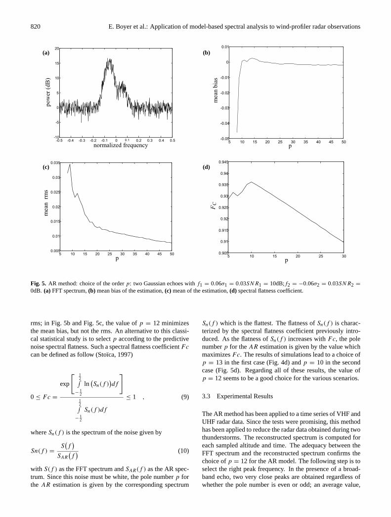
Fig. 5. AR method: choice of the orderp: two Gaussian echoes withf1 = 0.06σ1 = 0.03SNR1 = 10dB;f2 = −0.06σ2 = 0.03SNR2 =

0dB. (a) FFT spectrum,(b) mean bias of the estimation,(c) mean of the estimation,(d) spectral flatness coefficient.

rms; in Fig. 5b and Fig. 5c, the value ofp = 12 minimizesthe mean bias, but not the rms. An alternative to this classi-cal statistical study is to selectp according to the predictivenoise spectral flatness. Such a spectral flatness coefficientFc

can be defined as follow (Stoıca, 1997)

0 ≤ Fc =

exp

[ 12∫

−12

ln(Sn(f )

)df

]12∫

−12

Sn(f )df

≤ 1 , (9)

whereSn(f ) is the spectrum of the noise given by

Sn(f ) =S(f

)SAR

(f

) (10)

with S(f ) as the FFT spectrum andSAR(f ) as the AR spec-trum. Since this noise must be white, the pole numberp forthe AR estimation is given by the corresponding spectrum

Sn(f ) which is the flattest. The flatness ofSn(f ) is charac-terized by the spectral flatness coefficient previously intro-duced. As the flatness ofSn(f ) increases withFc, the polenumberp for theAR estimation is given by the value whichmaximizesFc. The results of simulations lead to a choice ofp = 13 in the first case (Fig. 4d) andp = 10 in the secondcase (Fig. 5d). Regarding all of these results, the value ofp = 12 seems to be a good choice for the various scenarios.

3.3 Experimental Results

The AR method has been applied to a time series of VHF andUHF radar data. Since the tests were promising, this methodhas been applied to reduce the radar data obtained during twothunderstorms. The reconstructed spectrum is computed foreach sampled altitude and time. The adequacy between theFFT spectrum and the reconstructed spectrum confirms thechoice ofp = 12 for the AR model. The following step is toselect the right peak frequency. In the presence of a broad-band echo, two very close peaks are obtained regardless ofwhether the pole number is even or odd; an average value,


rK

r( )t

r1 r2

∆Ts ∆Ts

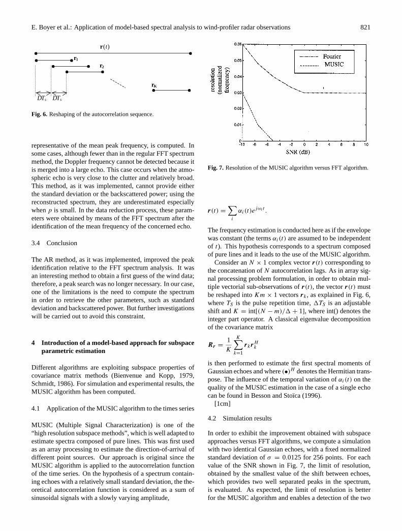
Fig.6 Reshaping of the autocorrelation sequence Fig. 6. Reshaping of the autocorrelation sequence.

representative of the mean peak frequency, is computed. Insome cases, although fewer than in the regular FFT spectrummethod, the Doppler frequency cannot be detected because itis merged into a large echo. This case occurs when the atmo-spheric echo is very close to the clutter and relatively broad.This method, as it was implemented, cannot provide eitherthe standard deviation or the backscattered power; using thereconstructed spectrum, they are underestimated especiallywhenp is small. In the data reduction process, these param-eters were obtained by means of the FFT spectrum after theidentification of the mean frequency of the concerned echo.

3.4 Conclusion

The AR method, as it was implemented, improved the peakidentification relative to the FFT spectrum analysis. It wasan interesting method to obtain a first guess of the wind data;therefore, a peak search was no longer necessary. In our case,one of the limitations is the need to compute the spectrumin order to retrieve the other parameters, such as standarddeviation and backscattered power. But further investigationswill be carried out to avoid this constraint.

4 Introduction of a model-based approach for subspaceparametric estimation

Different algorithms are exploiting subspace properties ofcovariance matrix methods (Bienvenue and Kopp, 1979,Schmidt, 1986). For simulation and experimental results, theMUSIC algorithm has been computed.

4.1 Application of the MUSIC algorithm to the times series

MUSIC (Multiple Signal Characterization) is one of the“high resolution subspace methods”, which is well adapted toestimate spectra composed of pure lines. This was first usedas an array processing to estimate the direction-of-arrival ofdifferent point sources. Our approach is original since theMUSIC algorithm is applied to the autocorrelation functionof the time series. On the hypothesis of a spectrum contain-ing echoes with a relatively small standard deviation, the the-oretical autocorrelation function is considered as a sum ofsinusoidal signals with a slowly varying amplitude,

Fig. 7. Resolution of the MUSIC algorithm versus FFT algorithm.

r(t) =

∑i

αi(t)ejωi t .

The frequency estimation is conducted here as if the envelopewas constant (the termsαi(t) are assumed to be independentof t). This hypothesis corresponds to a spectrum composedof pure lines and it leads to the use of the MUSIC algorithm.

Consider anN × 1 complex vectorr(t) corresponding tothe concatenation ofN autocorrelation lags. As in array sig-nal processing problem formulation, in order to obtain mul-tiple vectorial sub-observations ofr(t), the vectorr(t) mustbe reshaped intoKm × 1 vectorsrk, as explained in Fig. 6,whereTS is the pulse repetition time,1TS is an adjustableshift andK = int[(N − m)/1 + 1], where int() denotes theinteger part operator. A classical eigenvalue decompositionof the covariance matrix

Rr =1

K

K∑k=1

rkrHk

is then performed to estimate the first spectral moments ofGaussian echoes and where(•)H denotes the Hermitian trans-pose. The influence of the temporal variation ofαi(t) on thequality of the MUSIC estimation in the case of a single echocan be found in Besson and Stoıca (1996).

[1cm]

4.2 Simulation results

In order to exhibit the improvement obtained with subspaceapproaches versus FFT algorithms, we compute a simulationwith two identical Gaussian echoes, with a fixed normalizedstandard deviation ofσ = 0.0125 for 256 points. For eachvalue of the SNR shown in Fig. 7, the limit of resolution,obtained by the smallest value of the shift between echoes,which provides two well separated peaks in the spectrum,is evaluated. As expected, the limit of resolution is betterfor the MUSIC algorithm and enables a detection of the two


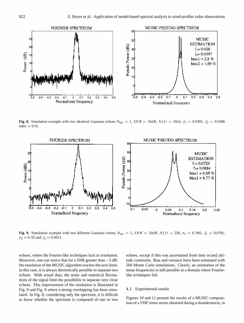
Fig. 8. Simulation example with two identical Gaussian echoesNinc = 1, SNR = 10dB, Nff t = 1024,f1 = 0.0391,f2 = 0.0586andσ = 0.01.

Fig. 9. Simulation example with two different Gaussian echoesNinc = 1, SNR = 10dB, Nff t = 256, σ1 = 0, 005, f1 = 0.0781,σ2 = 0, 02 andf2 = 0.0813.

echoes, where the Fourier-like techniques lack in resolution.Moreover, one can notice that for a SNR greater than−5 dB,the resolution of the MUSIC algorithm reaches the zero limit:in this case, it is always theoretically possible to separate twoechoes. With actual data, the noise and statistical fluctua-tions of the signal limit the possibility to separate very closeechoes. This improvement of the resolution is illustrated inFig. 8 and Fig. 9 where a strong overlapping has been simu-lated. In Fig. 8, considering only the spectrum, it is difficultto know whether the spectrum is composed of one or two

echoes, except if this was ascertained from time or/and alti-tude continuity. Bias and variance have been estimated with500 Monte Carlo simulations. Clearly, an estimation of themean frequencies is still possible in a domain where Fourier-like techniques fail.

4.3 Experimental results

Figures 10 and 11 present the results of a MUSIC computa-tion of a VHF times series obtained during a thunderstorm, in


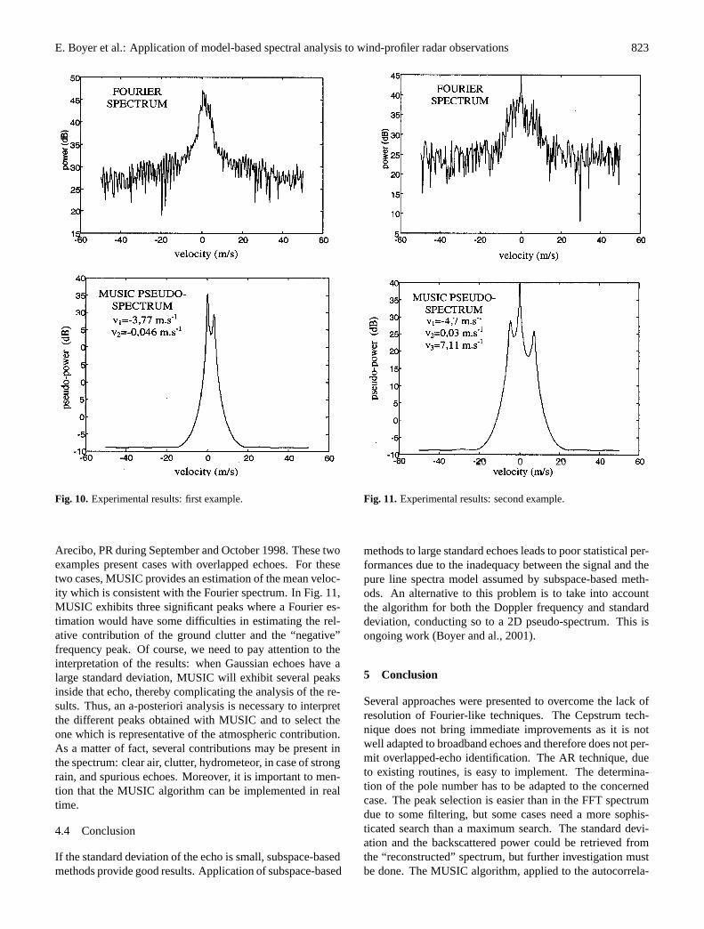
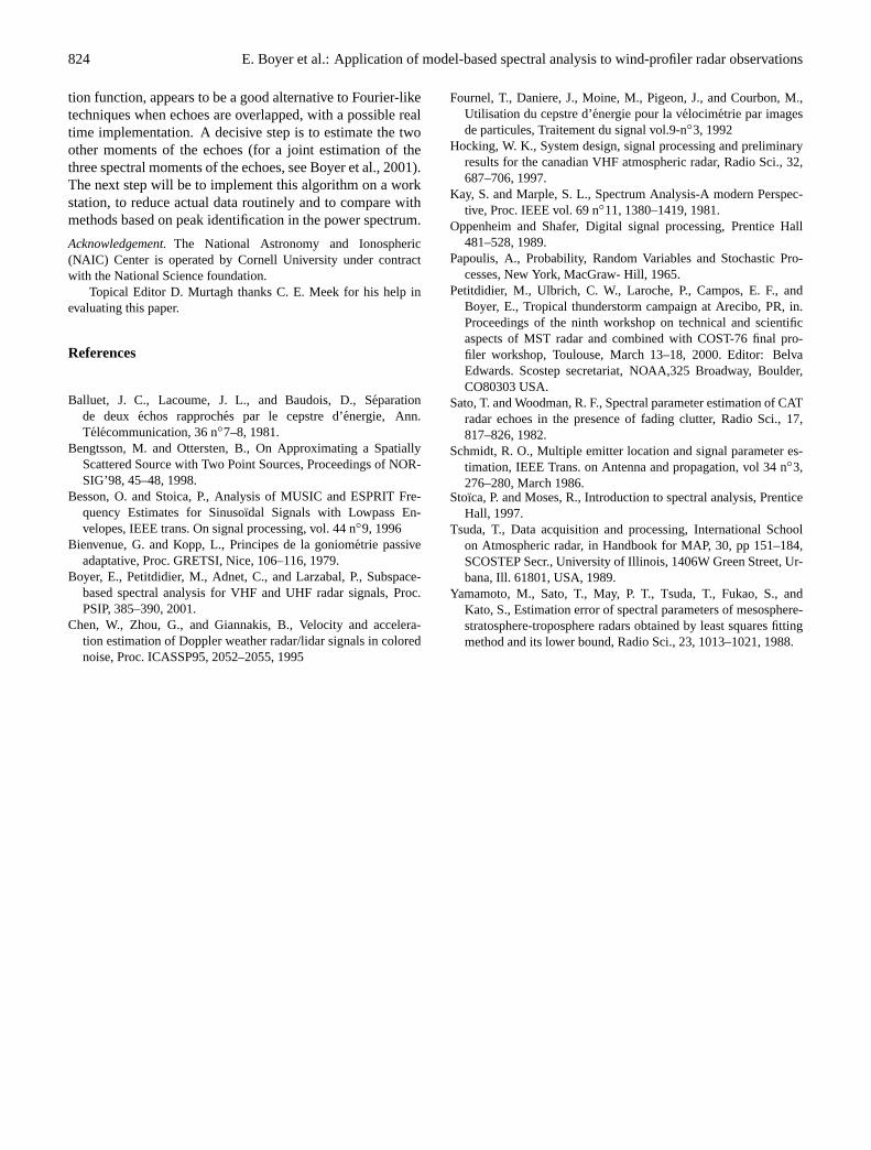
Fig. 10. Experimental results: first example.

Arecibo, PR during September and October 1998. These twoexamples present cases with overlapped echoes. For thesetwo cases, MUSIC provides an estimation of the mean veloc-ity which is consistent with the Fourier spectrum. In Fig. 11,MUSIC exhibits three significant peaks where a Fourier es-timation would have some difficulties in estimating the rel-ative contribution of the ground clutter and the “negative”frequency peak. Of course, we need to pay attention to theinterpretation of the results: when Gaussian echoes have alarge standard deviation, MUSIC will exhibit several peaksinside that echo, thereby complicating the analysis of the re-sults. Thus, an a-posteriori analysis is necessary to interpretthe different peaks obtained with MUSIC and to select theone which is representative of the atmospheric contribution.As a matter of fact, several contributions may be present inthe spectrum: clear air, clutter, hydrometeor, in case of strongrain, and spurious echoes. Moreover, it is important to men-tion that the MUSIC algorithm can be implemented in realtime.

4.4 Conclusion

If the standard deviation of the echo is small, subspace-basedmethods provide good results. Application of subspace-based

2020 0

Fig. 11. Experimental results: second example.

methods to large standard echoes leads to poor statistical per-formances due to the inadequacy between the signal and thepure line spectra model assumed by subspace-based meth-ods. An alternative to this problem is to take into accountthe algorithm for both the Doppler frequency and standarddeviation, conducting so to a 2D pseudo-spectrum. This isongoing work (Boyer and al., 2001).

5 Conclusion

Several approaches were presented to overcome the lack ofresolution of Fourier-like techniques. The Cepstrum tech-nique does not bring immediate improvements as it is notwell adapted to broadband echoes and therefore does not per-mit overlapped-echo identification. The AR technique, dueto existing routines, is easy to implement. The determina-tion of the pole number has to be adapted to the concernedcase. The peak selection is easier than in the FFT spectrumdue to some filtering, but some cases need a more sophis-ticated search than a maximum search. The standard devi-ation and the backscattered power could be retrieved fromthe “reconstructed” spectrum, but further investigation mustbe done. The MUSIC algorithm, applied to the autocorrela-


tion function, appears to be a good alternative to Fourier-liketechniques when echoes are overlapped, with a possible realtime implementation. A decisive step is to estimate the twoother moments of the echoes (for a joint estimation of thethree spectral moments of the echoes, see Boyer et al., 2001).The next step will be to implement this algorithm on a workstation, to reduce actual data routinely and to compare withmethods based on peak identification in the power spectrum.

Acknowledgement.The National Astronomy and Ionospheric(NAIC) Center is operated by Cornell University under contractwith the National Science foundation.

Topical Editor D. Murtagh thanks C. E. Meek for his help inevaluating this paper.

References

Balluet, J. C., Lacoume, J. L., and Baudois, D., Separationde deux echos rapproches par le cepstre d’energie, Ann.Telecommunication, 36 n◦7–8, 1981.

Bengtsson, M. and Ottersten, B., On Approximating a SpatiallyScattered Source with Two Point Sources, Proceedings of NOR-SIG’98, 45–48, 1998.

Besson, O. and Stoica, P., Analysis of MUSIC and ESPRIT Fre-quency Estimates for Sinusoıdal Signals with Lowpass En-velopes, IEEE trans. On signal processing, vol. 44 n◦9, 1996

Bienvenue, G. and Kopp, L., Principes de la goniometrie passiveadaptative, Proc. GRETSI, Nice, 106–116, 1979.

Boyer, E., Petitdidier, M., Adnet, C., and Larzabal, P., Subspace-based spectral analysis for VHF and UHF radar signals, Proc.PSIP, 385–390, 2001.

Chen, W., Zhou, G., and Giannakis, B., Velocity and accelera-tion estimation of Doppler weather radar/lidar signals in colorednoise, Proc. ICASSP95, 2052–2055, 1995

Fournel, T., Daniere, J., Moine, M., Pigeon, J., and Courbon, M.,Utilisation du cepstre d’energie pour la velocimetrie par imagesde particules, Traitement du signal vol.9-n◦3, 1992

Hocking, W. K., System design, signal processing and preliminaryresults for the canadian VHF atmospheric radar, Radio Sci., 32,687–706, 1997.

Kay, S. and Marple, S. L., Spectrum Analysis-A modern Perspec-tive, Proc. IEEE vol. 69 n◦11, 1380–1419, 1981.

Oppenheim and Shafer, Digital signal processing, Prentice Hall481–528, 1989.

Papoulis, A., Probability, Random Variables and Stochastic Pro-cesses, New York, MacGraw- Hill, 1965.

Petitdidier, M., Ulbrich, C. W., Laroche, P., Campos, E. F., andBoyer, E., Tropical thunderstorm campaign at Arecibo, PR, in.Proceedings of the ninth workshop on technical and scientificaspects of MST radar and combined with COST-76 final pro-filer workshop, Toulouse, March 13–18, 2000. Editor: BelvaEdwards. Scostep secretariat, NOAA,325 Broadway, Boulder,CO80303 USA.

Sato, T. and Woodman, R. F., Spectral parameter estimation of CATradar echoes in the presence of fading clutter, Radio Sci., 17,817–826, 1982.

Schmidt, R. O., Multiple emitter location and signal parameter es-timation, IEEE Trans. on Antenna and propagation, vol 34 n◦3,276–280, March 1986.

Stoıca, P. and Moses, R., Introduction to spectral analysis, PrenticeHall, 1997.

Tsuda, T., Data acquisition and processing, International Schoolon Atmospheric radar, in Handbook for MAP, 30, pp 151–184,SCOSTEP Secr., University of Illinois, 1406W Green Street, Ur-bana, Ill. 61801, USA, 1989.

Yamamoto, M., Sato, T., May, P. T., Tsuda, T., Fukao, S., andKato, S., Estimation error of spectral parameters of mesosphere-stratosphere-troposphere radars obtained by least squares fittingmethod and its lower bound, Radio Sci., 23, 1013–1021, 1988.

Documents

Geophysicae Application of model-based spectral … · Geophysicae Application of model-based spectral analysis to wind-proﬁler radar observations ... (Oppenheim and Shafer, 1989;