Embed Size (px)
Citation preview
J . FZuid Mech. (1989), vol. 198. p p . 557685
Printed in Great Britain
557
Geometry of self-propulsion at low Reynolds number
By ALFRED SHAPERE? AND F R A N K WILCZEKS t Institute for Advanced Study, Princeton, NJ 08540, USA
$ Institute for Theoretical Physics, University of California, Santa Barbara, CA 93106, USA
(Received 15 April 1987 and in revised form 12 July 1988)
The problem of swimming a t low Reynolds number is formulated in terms of a gauge field on the space of shapes. Effective methods for computing this field, by solving a linear boundary-value problem, are described. We employ conformal-mapping techniques to calculate swimming motions for cylinders with a variety of cross- sections. We also determine the net translational motion due to arbitrary infinitesimal deformations of a sphere.
1. Introduction It has been appreciated for some time that self-propulsion a t low Reynolds number
is an interesting fluid-dynamical problem of considerable biological importance (Taylor 1951). Dynamics at low Reynolds number has a rather special and unique character. The effects of inertia are negligible in this limit ; in the absence of driving forces, bodies are a t rest. For this reason, motion a t low Reynolds number has been called a realization of Aristotelean mechanics (Purcell 1977).
In the absence of inertia, the motion of a swimmer through a fluid is completely determined by the geometry of the sequence of shapes that the swimmer assumes. It is independent of any variation in the rates a t which different parts of the sequence are run through (as long as this rate is slow, of course).
The purely geometrical nature of the problem of self-propulsion at low Reynolds number suggested to us that there should be a natural, attractive mathematical framework for this problem. We believe that we have found such a framework. It is the subject of this paper.
We shall show, in $2, that the problem of self-propulsion a t low Reynolds number naturally resolves itself into the computation of a gauge potential field on the space of shapes. The gauge potential A describes the net translation and rotation resulting from an arbitrary infinitesimal deformation of a shape. It takes its values in the Lie algebra of rigid motions in Euclidean space. To find the translation and rotation of a swimmer which changes its shape along a given path in shape space, one computes the (path-ordered) integral of the gauge potential A along this path. We shall describe how to calculate A , in principle, by solving a linear boundary-value problem.
In two dimensions, there are powerful techniques which make explicit calculations of A quite practical for a wide range of shapes. The similarity between the equations of low-Reynolds-number hydrodynamics and of elasticity theory is well known (Rayleigh 1878). I n two dimensions, complex-variable methods developed in the context of elasticity theory (Muskhelishvili 1953) can be carried over almost without
558 A . Shapere and F . Wilczek
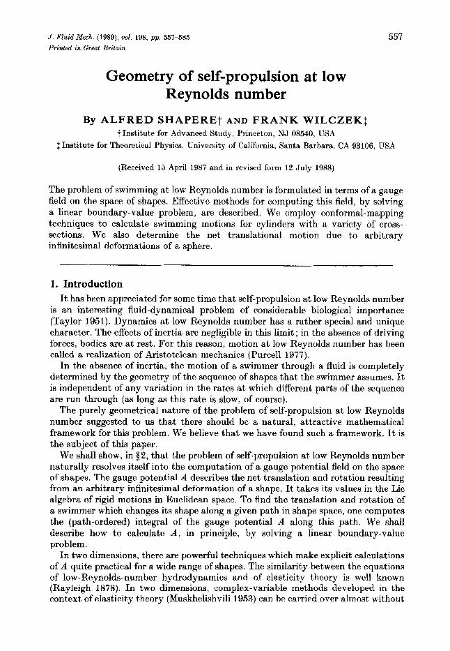
I k
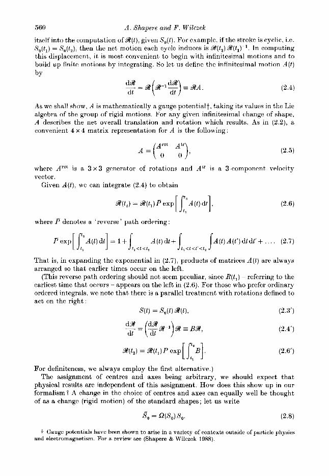
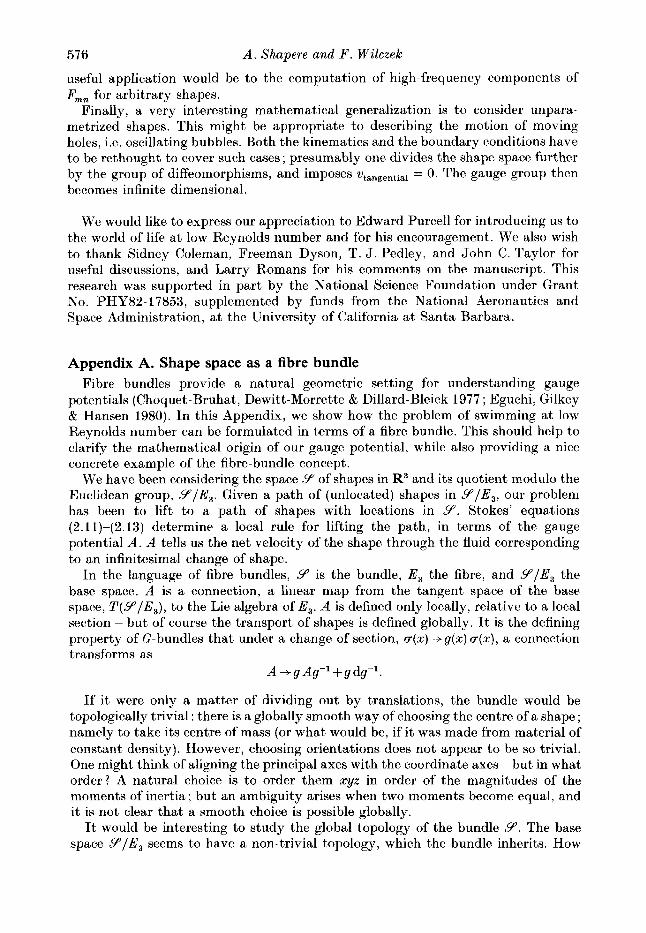
FIGURE 1. In order to measure distances between different shapes, an arbitrary choice of reference frames must be made.
modification (for a review, see Hasimoto & Sano 1980). These techniques are well- adapted to solving our boundary-value problem. The general procedure is outlined, and some examples are presented, in $3. Strokes involving infinitesimal deformations of a circle are analysed completely, as are finite deformations within a restricted space of shapes.
In $4 we discuss the swimming of a nearly spherical organism in three dimensions. Again, the case of infinitesimal deformations can be analysed completely, by using vector spherical harmonics to exploit the symmetry of the problem. In the final section, we discuss possible extensions of the work. Several appendices contain details of our calculations and discussions of mathematical topics.
The calculation of efficiencies, leading to the determination of optimally efficient strokes, is presented in a companion paper (Shapere & Wilczek 1989).
2. Kinematics 2.1. General framework; gauge structure
The configuration space of a deformable body is the space of all possible shapes. We should a t the outset distinguish between the space of shapes located somewhere in space and the more abstract space of unlocated shapes. The latter space may be obtained from the space of shapes cum locations by declaring two shapes with different centres of mass and orientations to be equivalent.
The problem we wish to solve may be stated as follows: what is the net rotation and translation which results when a deformable body goes through a given sequence of unoriented shapes, in the absence of external forces and torques 1 I n other words, given a path in the space of unlocated shapes, what is the corresponding path in the space of located shapes ? The problem is intuitively well-defined - if a body changes its shape in some way, a net rotation and translation is induced. The net motion may be found by solving Stokes’ equations for the fluid flow, with boundary conditions on the surface of the shape corresponding to the given deformation.
These remarks may seem straightforward enough, but as soon as we try to formulate the problem more specifically, we encounter a crucial ambiguity. The root problem in the kinematics of deformable shapes is displayed in figure 1. We wish to
Geometry of self-propulsion at low Reynolds number 559
compute the motion : how far has shape I moved, and how has i t reoriented itself, in the process of becoming shape 111 In this form, the question is clearly ill-posed. Different points on or inside of the boundary may have moved differently.
To quantify the motion, it is necessary to at,tach a centre and a set of axes to each unlocated shape, as in figure 1. This is equivalent to choosing a 'standard location ' for each shape; namely, to each unlocated shape there now corresponds a unique located shape, whose centre and axes are aligned with the origin and coordinate axes of physical space. Once a choice of standard locations for shapes has been made, then we shall say that the rigid motion required to move from I to I1 is the displacement and rotation necessary to align their centres and axes.
Now let r parameterize the boundary of a shape S(a), and let S,(a) be the associated standard shape. (For example, if S is a simply connected shape in three dimensions, we will take r = (e,#) to be a coordinate on the unit two-sphere, and S ( r ) to be a map from S2 into R3. For two-dimensional (cylindrical) shapes, it will prove to be most convenient to use the complex coordinate on the unit circle, r = cis.) Then
S ( r ) = WS,(r), (2.1)
where 9 is a rigid motion. We emphasize that S and So are parameterized shapes; different functions S ( r ) and S ' ( r ) correspond to different shapes, even if their images coincide geometrically.
To make (2.1) more explicit, we introduce a matrix representation for the group of Euclidean motions, of which W is a member. A three-dimensional rigid motion consisting of a rotation R followed by a translation d may be represented as a 4 x 4 matrix
where R is an ordinary 3 x 3 rotation matrix, d is a 3-component column vector, and 1 is just the I x 1 identity matrix. These matrices obey the correct group algebra
[ R , d'] [R, d ] = [R'R, Rd+d'],
[R,d]-l = [R-', -R-ld].
Vectors u on which [R,d] acts are represented as 4-component column vectors (v, l)T; then v+Rv+d. In the notation of (2.1), W = [R,d] acts on the vector (#,(a), l)T, for each r.
Now in considering the problem of self-propulsion a t low Reynolds number, we shall assume that our swimmer can squirm, but not pull itself by its bootstraps. That is, we shall assume it has control over its form (i.e. its standard shape, as defined above), but cannot exert net forces and torques on itself. A swimming stroke is therefore specified by a time-dependent sequence of forms, or equivalently standard shapes S,(t) (the r-dependence is implicit). The actual shapes will then be
S(t) = W(t)S , ( t ) , (2.3)
where 9 ( t ) is a time-dependent sequence of rigid displacements. Note that we allow shape changes which change both the volume and surface area in our general formulation. These may be constrained at a later stage, although we shall not consider such restrictions in this paper.
The dynamical problem of self-propulsion a t low Reynolds number thus resolves
560 A. Shapere and F . Wilczek
itself into the computation of 9 ( t ) , given S,(t). For example, if the stroke is cyclic, i.e. s,(t,) = s,(t,), then the net motion each cycle induces is 9 ( t , ) 9( t1 ) - l . In computing this displacement, it is most convenient to begin with infinitesimal motions and to build up finite motions by integrating. So let us define the infinitesimal motion A ( t ) by
(2.4)
As we shall show, A is mathematically a gauge potentialt, taking its values in the Lie algebra of the group of rigid motions. For any given infinitesimal change of shape, A describes the net overall translation and rotation which results. As in (2.2), a convenient 4 x 4 matrix representation for A is the following :
where Arot is a 3 x 3 generator of rotations and Atr is a 3-component velocity vector.
Given A(t), we can integrate (2.4) to obtain
where P denotes a ‘reverse’ path ordering:
Ponp[ [:A(t)dt] = I + l A(t)dt+J p ( t ) A ( t ’ ) d t d t ’ + . . . . (2.7) t l < t < t , t,<t <t‘<t,
That is, in expanding the exponential in (2.7), products of matrices A(t) are always arranged so that earlier times occur on the left.
(This reverse path ordering should not seem peculiar, since R(t,) ~ referring to the earliest time that occurs - appears on the left in (2.6). For those who prefer ordinary ordered integrals, we note that there is a parallel treatment with rotations defined to act on the right:
W) = d,(t) 9 ( t ) , (2.3‘)
(2.4’)
(2.6’)
For definiteness, we always employ the first alternative.) The assignment of centres and axes being arbitrary, we should expect that
physical results are independent of this assignment. How does this show up in our formalism 1 A change in the choice of centres and axes can equally well be thought of as a change (rigid motion) of the standard shapes ; let us write
t Gauge potentials have been shown to arise in a variety of contexts outside of particle physics and electromagnetism. For a review see (Shapere & Wilczek 1988).
Geometry of self-propulsion at low Reynolds number 56 1
The physical shapes being unchanged, (2.1) requires us to define
&(t) = 9 ( t ) Q-l(Eo(t)) . (2.9)
From this, the transformation law A and for the connecting path integral follow:
a = QAQ- l+Q- dt (2.10)
Readers familiar with gauge field theory will recognize these transformation laws. W implements a gauge transformation in the space of shapes ; A transforms as a gauge potential and W as a Wilson line integral. Our freedom in choosing the assignment of centres and axes shows up as a freedom of gauge choice on the space of standard shapes. The final relationship between physical shapes, i.e. E(t,) and s ( t , ) , is manifestly independent of such choices.
The appearance of a gauge structure in the context of low-Reynolds-number fluid mechanics is in fact quite natural. Generally, gauge structures are associated with large redundancies in the description of a physical system. Here, the redundancy is associated with our freedom to choose a standard orientation and location for each possible shape. This gauge structure is a general feature of the mechanics of deformable bodies without inertia.
The gauge potential A has a geometric origin. Namely, A may be viewed as a connection on a fibre bundle over the space of standard shapes. This point of view is discussed in Appendix A.
2.2. T h e dynamical problem : determining the gauge potential The dynamical problem of self-propulsion a t low Reynolds number has been reduced to the calculation of the gauge potential A . Here we outline an effective method for determining A . Later parts of the paper contain many specific examples.
First, let a sequence of forms 8,(t) be given. I n general, this sequence of forms does not in itself specify a possible motion according to our hypotheses, for it will involve net forces and torques on the swimmer. The allowed motion, involving the same sequence of forms, will include additional time-dependent rigid displacements. I n other words, the actual motion will be the superposition of the given motion sequence S,(t) and counterflows, corresponding to additional rigid displacements which cancel the forces and torques.
To calculate the counterflow, we solve for the response of the fluid to the trial motion Eo(t) . This is given by the solution to the boundary-value problem (Happel & Brenner 1965; Childress 1978)
v.v = 0, (2.11)
(2.12) vyv x v) = 0,
(2.13)
Equations (2.11) and (2.12) are the standard equations for incompressible flow a t low Reynolds numbers, and (2.13) is the no-slip boundary condition. I n interpreting (2.13), it is important to remember that the E,(t) are really parametrized shapes E o ( c , t ) , and that the variation is meant to be taken with
The force and torques associated with the trial motion can be inferred from the fixed.
562 A . Shapere and F . Wilczek
asymptotic behaviour of v at spatial infinity. The force on the shape is related to the external force on the fluid a t spatial infinity, a,nd thence to the asymptotic flow, by thc conservation of momentum. Indeed, if uij is the stress tensor then the force on the shape is (Ratchelor 1970)
F, = 1 %ja8j> shape
but the stress tensor is conserved, a,a, = 0, so this is n
Now the stress tensor is given in terms of the velocity, and only the terms that fall off slowly and have the right symmetry survive. In fact, we shall show in $4 that the force is linearly related to the leading term in the asymptotic flow. A similar argument, leading to a similar conclusion, can be made for the torque.
To cancel these forces and torques, we must correct the motion by subtracting a Stokes’ flow corresponding to a rigid displacement of the shape with the same leading behaviour a t infinity as our trial solution. The result is the actual fluid motion. By our definition, this rigid displacement is
1 x A ( t ) st. (2.14)
This completes our outline of the method for calculating A . Thus far, we have treated A as a time-dependent quantity. However, the
geometric nature of our problem suggests that it should be possible to formulate an answer to i t in a completely time-independent way, i.e. to express the integrand in (2.6) in a manner that makes no reference to a time coordinate. Accordingly, we can define an abstract vector field over shape space, which we shall also denote by A , whose projection onto the direction SS,/Gt a t the point s,(t) is just A ( t ) :
= A.So[S,(t)l. (2.15)
Then the integral of (2.6) is equal to the line integral of A over the path S,(t) in shape space. and is manifestly independent of how this path is parameterized :
9 ( t 2 ) = 9 ( t l ) P exp [ l::l:: A[S’,] d&] . (2.16)
A may have infinitely many components, one for each direction of shape space, and each of which is a generator of a rigid motion. In terms of a fixed basis of vector fields {w,} over Yo, we may define components A,[S,] = A,,[S,].
2.3. Two corollaries
We now pause to discuss two simple but notable general properties of self-propulsion a t low Reynolds number, which are particularly easy to appreciate in our framework.
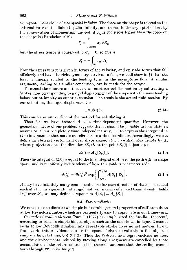
Generalized scallop theorem Purcell (1977) has emphasized the ‘scallop theorem ’, according to which a simple hinged object such as the one shown in figure 2 cannot swim a t low Reynolds number. Any repeatable stroke gives no net motion. In our framework, this is evident because the space of shapes available to this object is simply a bounded line, 0 < 0 < 2 ~ . Thus the Wilson line integral encloses no area, and the displacements induced by moving along a segment are cancelled by those accumulated in the return motion. (The theorem assumes that the scallop cannot turn through 2x on its hinge!)
Geometry of self-propulsion at low Reynolds number 563
FIGURE 2. A simple hinged animal with one degree of freedom cannot swim.
Helix theorem One cycle of a swimming stroke results in a definite displacement, i.e. translation and rotation. Repeating this cycle will lead to the square of the displacement, and so forth. The result is that the swimmer will trace out a generalized helix. To put i t more precisely, a true helix is described by
x( t ) = exp (ta) x(O), (2.17)
where a is in the Lie algebra of rigid motions, the infinitesimal displacement which generates the helix. A generalized helix, in our sense, is described by
z ( t ) = exp (ta) R(t) x(O), (2.18)
where R(t) is some periodic function, with R(T) = R(0) = 1. The proof is as follows. Let the period of the cyclic motion be one time unit, and let the rotation and displacement due to one stroke be
expa = P e x p [ S,’.dt].
[ Lt, A Then P exp[ [ A dt = exp (ta) exp ([t l- t) a P exp
= exp (ta) R(t),
where [t] denotes the greatest integer < t . Many swimming micro-organisms have indeed been observed to follow helical
trajectories. Some examples of helical paths for flagellar swimmers have been computed and compared with observations by Keller & Rubinow (1976). Helices are ubiquitous in biology ; we suspect the mathematical reason is this theorem.
In two dimensions, the helix theorem takes on a peculiar form. It says that cyclic swimming strokes can only lead to net motions which are ‘generalized circles’. That is, orbits of the Euclidean group E2 are circles, and the path of a swimmer will in general be a sort of a squiggly polygon described by (2.18). Motidn of this type is depicted in figure 4. In order for the swimmer to avoid going around in circles, the net displacement per cycle must be a pure translation.
2.4. InJinitesimal deformations The case of infinitesimal deformations of a shape is sufficiently important and interesting that it deserves separate comment.
Let the standard shapes be parametrized by
&,(t) = X,+s(t), (2.19)
where the s(t) are infinitesimal. We expand s(t) in terms of a fixed basis of vector fields on S o :
s ( t ) = Ca,(t) wi. (2.20) i
564
Then we have for the velocity on #,(t):
A. Shapere and P. Wilczek
Xow let us expand the gauge potentials to second order :
(2.21)
(2.22)
In the path-ordered exponential integral (2.7) around a cycle, which is the basic object giving the net displacement, the first-order term gives no contribution, for i t is a total derivative. The second-order contributions are terms quadratic in A and lincar in its derivatives. Because (2.7) is gauge covariant for a cyclic path, its Taylor expansion in powers of s ( t ) must also be gauge covariant, order by order. In fact, there is a unique (up to normalization) second-order gauge covariant term we can form, which is antisymmetric in the indices i and j:
(2.23)
The physical significance of Elwiwj is as follows. Suppose we make a sequence of successive deformations of So by cwi, rwj, -ewt, and -ywj. Finally, we close the sequence of shapes with the Lie brackct - q [ w i , uij]. Then the nct displacement will be erFwtwj . This makes it clear why F must be antisymmetric in its indices, so that thc reverse sequence of shapes gives the reverse displacement.
It is easily verified that expansion of (2.7) to second order gives
P exp [ f A dt] = 1 + f f C Fwiwj ai ci j dt. i j
(2.24)
The field strength tensor, evaluated a t a shape So, thus encodes all information on swimming motions due to arbitrary infinitesimal deformations of So.
3. The two-dimensional problem 3. I . Two-dimensional techniques
We shall now apply the techniques described in $2 to study the swimming motion of extended bodies a t very low Reynolds number. In this section, we restrict our attention to t)he admittedly unbiological example of an infinitely long cylindrical body of constant cross-section. The boundary-value problem (2.11)-(2.13) then becomes effectively two-dimensional, and may be solved by techniques of complex analysis. The solution is qualitatively similar to the three-dimensional case, yet easier to obtain and to interpret.
After setting up the machinery for handling the general two-dimensional problem, we shall apply it to the computation of the swimming motions of cylinders with some simple cross-sectional shapes. We shall also compute the field strength tensor for a cylinder with circular cross-section, leading to a description of all swimming motions of nearly circular cylinders.
Geometry of self-propulsion at low Reynolds number 565
In $2, we found the set of equations that must be satisfied by the velocity field v a t low Reynolds number:
v . u = 0, (3.1)
(3.2) V2(V x u) = 0,
ax ul, = t’ (3.3)
Let us suppose that the shape S is a cylinder and that the velocity field v contains no z-component, so that the boundary-value problem is two-dimensional. Then the first equation implies that the two-component vector u is the curl of a scalar potential U (possibly multivalued), and
v x v = v x (V x U ) = -v2u. J Thus U , by (2.2), satisfies the biharmonic equation,
v4u = 0. (3.5)
This equation has been extensively studied in the theory of elasticity in two dimensions. In elastic boundary-value problems, the second partial derivatives of U represent the stresses on an elastic medium (Rayleigh 1878; Hill & Power 1955). Muskhelishvili (1953) (see also England 1971) has applied methods of complex analysis to these problems, with elegant results. His methods have proved equally useful in the context of low-Reynolds-number fluid mechanics (Richardson 1968 ; Hasimoto & Sano 1980).
One reason complex analysis is so useful in solving the biharmonic equation is that biharmonic functions have a simple representation in terms of analytic functions. Namely, any U satisfying (3.5) may be written in the form
+U(Z, q = ~ $ ( z ) + z ~ + @ ( z ) + 1 C r ( z ) , (3.6)
where $ and II. are analytic in z = x+iy. As a corollary, we obtain an important representation for the velocity field, written as u = u,+ivy,
~~
= $lW -z$’,(z, + $&,. (3.7)
To discuss the swimming of shapes, we wish to consider an external boundary- value problem for U , with u = V x U specified on the exterior boundary of a compact region in the plane. Let s represent the complex coordinate z restricted to the boundary. Then given u(s), we wish to find functions $1, $2 analytic in the exterior of s such that
4 s ) = % w - s m + m . (3.8)
The problem is easily solved if S is a circle - we simply equate Fourier coefficients on both sides of (3.8). Although the result has been derived elsewhere (Muskhelishvili
566 A . Shapere and F . Wilczek
1953), we shall present a derivation in order to establish notation. Suppose we have Fourier expansions
m
v(s ) = c vlcsk+l, k=-m
(3.9)
where s = eie. (Summation over non-positive k ensures that $ ] ( z ) and #,(z), and consequently v(z), are finite at infinity. We may take bk, = 0 without loss of generality.) Then (3.8) is equivalent to
m
2 WkSk+1 = c akSk+l- c ( k + 1) ciks-k+l + c liks-k-1, k--w k<O k<O k<-1
since s-l = S. The complete solution is
a, = vk
b-, = co,
(k: < O ) ,
bk = f l . - k - 2 + ( k + 3 ) V k + 2 ( k < -2).
Thus the solutions with v ( s ) = Aszf1 on the circle correspond to
(3.10)
$hl(s) = 0, $2(s) = xs-l-' (1 > - 11, (3.11)
$1(4 = = 0 (I = - l), (3.12)
$h1(s) = Aslfl , $,(s) = h(Z+ 1) 81-1 (1 < - 1). (3.13)
These may be extended to the entire region of flow, i.e. the exterior of the circle, by substituting s+ z and using the representation (3.7). The results are
= Az- l - l (1 > - I ) , (3.14)
v = A ( I = - l ) , (3.15)
v = Az~+l-X(Z+ 1) zl-l(%z- 1) (3.16)
This is the complete solution to the boundary-value problem (3.8) when X is a circle.
For those who prefer two-component vector notation, we can successively take h real or imaginary in (3.14)-(3.16) to obtain a basis of equivalent solutions
( I < - 1).
for 12 -1, (3.17) 1 v i ( r , 0) = r-'-l(cos (Z+ 1) 8, sin ( Z + 1) B ) , v:(r,O) = ~ ~ - ' ( - s i n ( i + 1 ) 8 , cos(Z+1)8)
v; = r l+ l (cos ( I + 1) B - (Z+ 1) (1 -r+) cos ( I - 1) 8, and
for I < - 1. (3.18) I sin (1 + 1) B + (1 + 1) ( 1 - T + ) sin (1 - 1) B ) , v 2 - - r I f 1 ( - s i n ( I + l ) 8 + ( Z + l ) ( l - r ~ z ) s i n ( I - l ) ~ ,
Geometry of self-propulsion at low Reynolds number 567
It will prove useful to form combinations with definite helicity (i.e. simple properties under rotation)
( 1 2 - 1)
1 -(z+1)(1-r-z) eki(r-l)Op d2 (1 , f i ) I ( 1 < - 1). (3.19)
(It should be kept in mind that the i appearing in (3.19) is not the same as in z = z+iy.) Rotation through a changes these flows by
wt + ekizaw$. (3.20)
We say that wlk has helicity f l . Note that the solutions (3.15) corresponding to translations of the circle involve
rigid motion of the fluid as a whole. (Solutions corresponding to rigid rotations ( 1 = 0 and Ih( = 1) fall off slowly, like ~ l . ) This unphysical behaviour is known as Stokes’ paradox, and is a well-known peculiarity of two-dimensional low-Reynolds-number hydrodynamics. Because of our requirement that the external forces and torques vanish, we never encounter these rigid motions of the circle - in fact we determine the gauge potentials precisely by ‘subtracting them off’. The fact that, math- ematically, rigid motions of the circle give rise to such long-range motions of the fluid is actually a convenience, since it allows us to identify the necessary counterflows, i.e. the gauge potentials, very easily from the asymptotics of a trial flow at infinity. (As we shall see, the story is different for non-circular shapes, and for three-dimensional spheres.)
3.2. Nearly circular shapes
Before continuing to build up the general formalism, we pause to work out the important example of nearly circular shapes in detail. This computation has been done previously by Blake (1971 b) , in the case of irrotational strokes symmetric about the axis of propulsion.
To compute the field strength tensor, F , which governs the motion resulting from infinitesimal deformations, we must consider closed paths in two-dimensional sub- spaces of shape space. Let wl, w2 be two velocity fields on the circle and let W(swl, v w z ) be the rotation and translation of the circle induced by the following sequence of motions, as depicted in figure 3:
s +s + EW1 +s+ EVl + vvz -+s + ?pz +s. (3.21)
We work to second order in E , Y . Then, by (2.24),
W(EZ.’1,7%) = [ l I o l + M v l v p (3.22)
Fv,vl lies in the Lie algebra of rigid motions. F is most easily computed by matching the boundary condition Tv,(B) on the surface of the circle deformed by ewl(O). If we
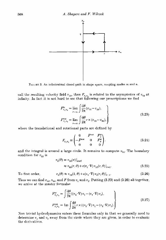
568 A . Shapere and F . Wilczek
an
I FIGURE 3. An infinitesimal closed path in shape space, coupling modes m and n.
call the resulting velocity field vI2, then F,'.,,, is related to the asymptotics of w12 at infinity. In fact it is not hard to see that following our prescriptions we find
where the translational and rotational parts are defined by
0 Frat FF F, , = -Frat 0 F:).
1 2 ( 0 0 0
(3.23)
(3.24)
and the integral is around a large circle. It remains to compute vIz. The boundary condition for w12 is
V2(6') = w12(4 lsurf
= v12(r, 6 ) + d W l . V ) %z(r, 6 ) 17=1. (3.25)
To first order, w2(6 ' ) = v,2(1,6')+€(:(v;V)v,(r,B) Ll. (3.26)
Thus we can find wI2, w21, and F from wl and w2. Putting (3.23) and (3.26) all together, we arrive a t the master formulae
(3.27)
Non-trivial hydrodynamics enters these formulas only in that we generally need to determine v1 and w2 away from the circle where they are given, in order to evaluate the derivatives.
Geometry of selj- propulsion at low Reynolds number 569
(It is worth remarking that the formulas (3.27) for the gauge field strength can be generalized to describe tangential deformations of an arbitrary shape. The argument preceding (3.27) implies that
where [ % W Z l = ( V , ~ V ) ~ 2 - ( ~ z ' V ) V 1
is the Lie bracket. Thus the complete field strength is
Fv1v2 = A,v1,v2,+[4J1,AvJ.
For the circle and sphere the second term vanishes - but it does not in general. When both v1 and w2 are tangential fields, the Lie bracket may be evaluated completely in terms of their values on the shape, with no hydrodynamics. Thus for purely tangential motions - reparametrizations of the boundary, which do not change the bulk shape - the form of A determines F directly.)
After these preliminaries, it is now a matter of straightforward algebra to insert the vector fields (3.19) into the master formula and thus derive F. The results for the translational part are as follows :
1 Ftr+ + = - [ - (m + 1) 8-, S,+,+, e- + (n + 1) en am+,+, e-
4 2 m n
+ (m+ 1) 8-, am+, e+- (n+ 1) 8-nS-m+n-le-], (3.30)
(3.31)
where e , = ( 1 / 4 2 ) (1 , k i ) , and 8, is zero for negative n and 1 for non-negative n. It is understood here that the + and - labels refer to the solutions wf in (3.19). The matrix F is antisymmetric ; apart from this all components of F whioh do not appear explicitly in (3.28)-(3.31) vanish. It is of course no accident that the vast majority of the components of F vanish in the helicity basis. Under a rotation through a, wf is multiplied by the phase in (3.20), while e + +e*ine+. Since F is linear in its arguments, and everything about our problem &I symmetric under rotations, this leads directly to constraints on which components of F may be non-zero.
F t r - + = -Ftr+ n m j - m n
For the rotational part of F we find
F ' O t m+n+ = - [ ( m + 1 ) 8, - (n+ 1) O n ] Sm+,, (3.32)
F',Otn- = [(m+1)8,-(n+l)8,]Sm+,, (3.33)
Fro$ m n - = - I m +1lSm-n , (3.34)
Fro! m n + = -F;jm-. (3.35)
570 A . Shapere and F . Wilczek
An alternative method for computing the components of the field strength, using complex variables throughout, is presented in Appendix B. In Appendix C, we discuss an interpretation of F,, in terms of the Virasoro algebra of conformal deformations.
3.3. Large deformations In the preceding section, we computed the net translation and rotation of a nearly circular cylinder due to an infinitesimal closed sequence of deformations. Here, we shall perform a complementary calculation for deformations of finite size. This will provide a concrete application of the gauge potential formalism we introduced in $2. Because the complexity of the calculation increases with the complexity of the deformations, we shall restrict attention to shapes described by conformal maps of the unit circle with degree D Q 2. (The extension to shapes of arbitrary degree will be discussed later.) A sequence of such deformations may be parameterized as
S(cr,t) = ao(t) a+a-,(t) a-l+a_,(t)a-2 (3.36)
where CT = cis. Here we have taken = 0 to 'fix the gauge' with respect to translations. We may also choose orientations for the standard shapes by requiring a,, to be real and positive. Note that a, must vanish if the analytic extension of S to the region of flow is to be conformal a t infinity.
To compute the translation and rotation due to the sequence of deformations (3.36), we need to solve the boundary-value problem (3.8) on the exterior of each of the shapes X(u, t ) for 0 Q t < T. This is most easily accomplished by conformally mapping the exterior of S(u, t ) in the z-plane onto the exterior of the unit circle, using z = S(5). Pulled back to the unit circle 5 = u in the 5-plane, (3.8) becomes
(3.37)
where o * ( a ) = v(S(a)) and $:, ,(a) = $1, 2(S(a)). (The asterisk here denotes a pull-back of q5, not complex conjugation.)
We may now solve for $:(c,t) and $ ? ( C , t ) . Then, if we want to know the actual fluid velocity field, we map back to the physical z-plane to obtain $1,2(z) = $T,,(X-'(z)) and use (3.7) to find v(z). More precisely, suppose that we have Laurent expansions in the 5- and z-planes
(3.38)
(3.39)
(3.40)
(3.41)
(3.42)
z a-2
010 z 5 = X-'(z) = ----+. . . . (3.43)
Geometry of self-propulsion at low Reynolds number 57 1
Then we solve for a,* and b,* by equating Fourier components in (3.37) and use S-l(z) to express a, and b, linearly in terms of a: and b,*. For example, the lead- ing coefficients a_, and b-, are
a_, = a-1, * (3.44)
b-, = a, b-,. * (3.45)
These are in fact the only coefficients we need in order to compute the gauge potential
As[S(a, t)l (3.46)
and consequently the net velocity of the shape a t time t . To proceed, (3.37) gives the following four equations for the leading a: and b,*
coefficients
(3.47)
(3.48)
1 a_, u-, = a*, u-,,
a_, u-l = a', u-l,
0 = a*, + Cc;la_, fz',, -
a, u = (b', + @;la-, a', + 2Cc;k3 a!,) u.
These may be solved to yield -
b-, = CI, b', = 0 1 ~ a, - Z-, - 2&, 4 a_, = a!, = - 2a;la-, &,,
since a, is real. The constant component of the fluid flow at infinity must be zero in order for the
net force on the shape to vanish. So we subtract from our solution v(z ) a counterflow up,, leading to a net translation velocity for the cylinder of
At' = B,. (3.49)
Similarly, after some algebra involving the equations of motion, the net torque is found to be
= lim r,p Re [ / .~gdZ] r0+m
= 8np Im (b-,). (3.50)
We can cancel this torque with a rotational counterflow of angular velocity w
(3.51)
such that, from (3.48),
Im (b-,) = Im (iw[la,12 + la-,I2 + 21a-,I2]}. (3.52)
Solving for w and using (3.48) we find then net rotational velocity of the shape
(3.53)
19 FLM I90
572 A . Shapere and F . Wilczek
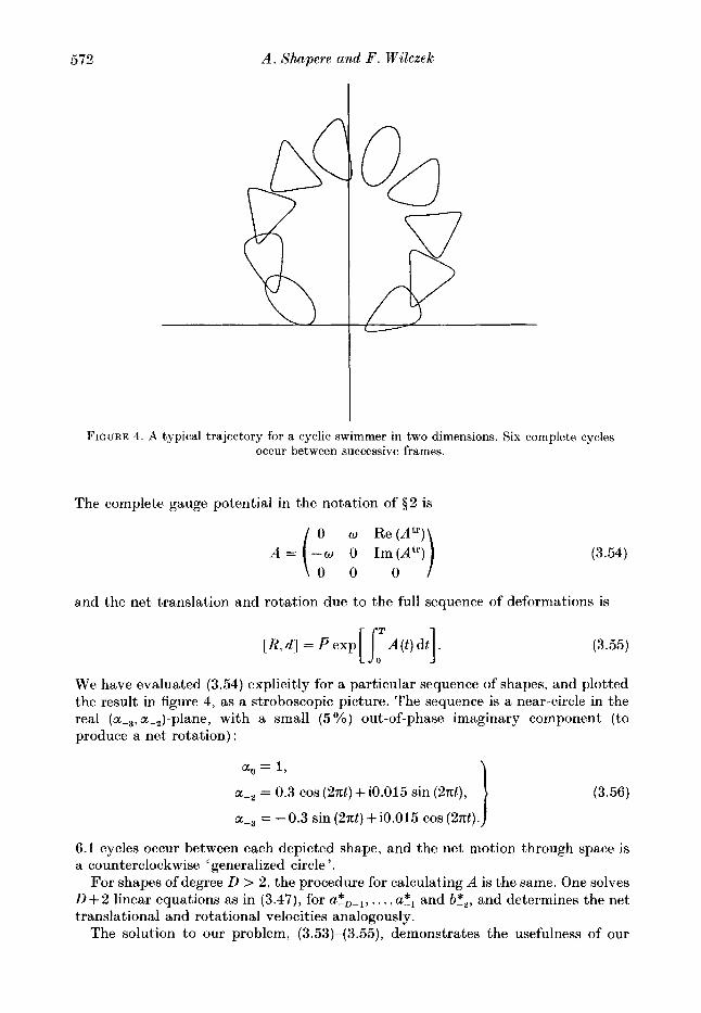
FIGURE 4. A I
typical trajectory for a cyclic swimmer in two dimensions. Six complete occur between successive frames.
The complete gauge potential in the notation of $ 2 is
0 o Re(Atr)
0 0 0 --w 0 Im(Atr)
cycles
(3.54)
and the net translation and rotation due to the full sequence of deformations is
[ R , d ] = P e x p [ S f A ( t ) d t ] . (3.55)
We have evaluated (3.54) explicitly for a particular sequence of shapes, and plotted the result in figure 4, as a stroboscopic picture. The sequence is a near-circle in the real (a-3, a-,)-plane, with a small (5 %) out-of-phase imaginary component (to produce a net rotation) :
a, = 1,
a-2 = 0.3 cos ( 2 x t ) + i0.015 sin (2x t ) , (3.56)
a-3 = -0.3 sin (2x t ) +i0.015 cos (2nt). J 6.1 cycles occur between each depicted shape, and the net motion through space is a counterclockwise ‘generalized circle ’.
For shapes of degree D > 2, the procedure for calculating A is the same. One solves D+2 linear equations as in (3.47), for aiD-l , . . . , a!, and b i z , and determines the net translational and rotational velocities analogously.
The solution to our problem, (3.53)-(3.55), demonstrates the usefulness of our
Geometry of self-propulsion at low Reynolds number 573
kinematic framework, and shows why it is necessary to introduce A in order to compute the net rigid motion. In fact, any solution to the problem we have posed in this section must be given by a path-ordered exponential integral over shape space, of a quantity which transforms under changes of reference axes for shapes as a gauge potential.
4. Squirming spheres We now wish to study the possible swimming motions of a nearly spherical
deformable body. This is a problem of some relevance in the biophysics of animal locomotion (Lighthill 1952 and Blake 1971 a) . In particular, consider a spherical animal which swims by waving a layer of short, densely packed cilia. (For reviews on the subject of self-propulsion of ciliated micro-organisms, see Blake & Sleigh 1975 ; Brennen & Winet 1977; Childress 1978; Lighthill 1975; Jahn & Votta 1972; Pedley 1975). An exact determination of all the swimming motions of such an animal would be impractical. However, we can usefully approximate the shape of this animal by a quasi-sphere, whose boundary just encloses the cilia. This approximation is known as the envelope model, and it is valid in the dual limit of short cilia relative to the radius of the sphere and dense packing relative to the lengths of the cilia. Paramecia, for example, are shaped like elongated spheres of length 200-300 pm (Blake & Sleigh 1975). The cilia are roughly 10 pm long and spaced 2 pm apart over the surface of the organism. Waves produced by the synchronous beating of the cilia are observed to have a frequency of about 30 Hz and a wavelength of 10 pm. The resulting helical trajectory is traversed with a velocity which has been observed to be between 600 and 2500 pm/s. While Paramecia are far from perfect spheres, one might hope to obtain at least, a qualitative understanding of their swimming patterns. We also expect that our methods can be extended to encompass simple non-spherical shapes such as ellipsoids.
The problem of determining all swimming motions of such an animal lends itself perfectly to solution within the framework we have developed. Namely, if we know the 'field strength tensor' F a t the sphere (which we may take to be of unit radius), then we know everything. The computation of F(S2) parallels that for the cylinder. We first find the general solution of the Navier-Stokes equations as an expansion in terms of vector spherical harmonics. We then solve the boundary-value problem for a slightly deformed sphere and obtain F,, from the asymptotic behaviour of this solution. We shall ignore any constraints on the volume or surface area of the quasi- sphere, other than the limits imposed by the lengths of the cilia.
Since our boundary conditions for the flow v are going to be on the surface of a unit sphere, it is appropriate to expand v in vector spherical harmonics:
The Y J L M are defined in terms of ordinary scalar spherical harmonics by 1
G L M = c c YLM<Lmlq ILIJM) e"q1 14.21
where &+, = T ( & z k i & u ) / 4 2 , e", = kt , and (LmlqILlJM) is a spin-1 Clebsch-Gordan coefficient.
We now insert the expansion of (4.1) u into the Navier-Stokes equations (2.11) and (2.12) to find k as a function of JLM. Using standard formulas for the Laplacian, curl,
m q=-1
10-2
574 A . Shapere and ill. Wilczek
and divergence of f ( r ) YJLM (see Appendix D) it is straightforward to show that (Lamb 1895)
This expansion should be compared with its two-dimensional analogue, given by (3.14)-(3.16). It is easily checked that the boundary-value problem of matching u with an arbitrary velocity field on a surface is well-determined.
The net velocities due to a given change in shapc are found, as in the two- dimensional case, from the condition that the net force and torque on the shape vanish. In fact, the net force and torque are proportional to leading asymptotics of u, of order r-l and rP2. To see this, recall that the net force is the surface integral of the fluid stress tensor over the boundary of the shape (Batchelor 1970):
By the divergence theorem and the fact that t..utj = 0 (Stokes’ equations), this is equal to the integral of uij over a large sphere of radius r
= Is, utj ?ij r2 dQ, (4.5)
where ?ij is a unit outward normal to the sphere. As r + m, the only piece of uij which survives in the integral is the term proportional to rP2, which comes from the term
C1M r-l KOM (4.6)
in (4.3). Thus, if our solution u contains such a piece, we must subtract it as a ‘ counterflow ’ in order to satisfy F = 0. The resulting net translational velocity of the shape is accordingly
Vtrans = - C l q e g . (4.7a)
(Here and henceforth, we sum implicitly over q = - l , O , 1 . ) Similarly, the rotation velocity comes from the term in the expansion of u proportional to Y O l M :
%t = aoqeq. (4 .7b )
To compute the translational components of the field strength, we follow the same procedure as in our earlier two-dimensional calculation, leading to the master formula of (3.27). The computation is presented in detail, and compared to earlier results of Blake, in Appendix E. We obtain
(4.8) - {JLM * J’L’M’},
Geometry of selj-propulsion at low Reyn,olds number 575
It is worth remarking on the similarity of this result to the field strength FZn of a circular cylinder, found in $3.2, First, the only non-zero components of F in either case correspond to pairs of modes which are connected by a two- or three- dimensional angular momentum operator. I n the three-dimensional case, this is a consequence of the spherical symmetry of the sphere. Thus, if the sphere is rotated by some J - h , then the translation d due to F must rotate similarly. Rephrasing the argument given in $3.2 for the cylinder now shows that J and J' must differ by a t most 1 in order for the sphere to translate.
A second similarity is that F,LM, J r L , M , grows linearly with J , for large J . This shows that the swimming motions of spheres and cylinders arc quantitatively as well as qualitatively similar, a conclusion which presumably extends to other shapes as well.
The computation of FYiM, J,L'M, is similar, although somewhat more involved. Frot is certainly essential in determining the helical motion which results from an arbitrary periodic swimming stroke. However, we expect that any maximally eficient stroke will involve no rotation (see Shapere & Wilczek 1989).
5. Summary and concluding remarks This paper provides a general kinematic framework for discussing self-propulsion
a t low Reynolds number. We have formulated this problem in terms of a gauge potential A , which gives the net rigid motion resulting from an arbitrary change of shape. Finite motions due to a sequence of changes of shape are given by a path- ordered exponential integral of A along a path in shape space, and cyclic infinitesimal swimming motions are described by the covariant curl F of A . We have discussed an algorithm for determining A a t shapes related to the circle by a conformal map of finite degree, and evaluated A explicitly for all deformations of conformal degree two. Our computations of the field strength of the circular cylinder and of the sphere effectively determine all possible infinitesimal swimming motions of these shapes.
Knowing, as we now do, the motion that results from any infinitesimal cyclic swimming stroke around a circle or a sphere, we may try to find the most efficient strokes. We analyse this problem in an accompanying paper (Shapere & Wilczek 1989). Qualitatively, we find that optimal infinitesimal strokes are wave-like motions symmetric about the axis of propulsion. The waves propagate from front to rear (relative to the direction of motion), achieving a maximum amplitude near the middle.
There are several other directions in which our work should be extended: It should be possible, following the methods of Muskhelishvili, to calculate F for
a variety of two-dimensional shapes, e.g. ellipses. It is quite possible that there is a fairly direct algorithm of calculating F for any conformal image of the circle ; we have not examined this closely. In three dimensions, it would be biologically interesting to extend our calculation of F for the sphere to prolate spheroids, by expanding the flow in prolate spheroidal harmonics.
The similarity of the field strengths of the cylinder and the sphere in the high- frequency limit suggests a possible approximation which could apply to arbitrary shapes. Since the flows generated by high-frequency disturbances on the boundary tend to die rapidly with distance, it should be possible to treat them approximately for any shape, by replacing the shape locally with its tangent plane. Such an approximation has been mentioned in the literature (Childress 1978 and references therein), although, to our knowledge, a firm mathematical justification is lacking. A
576 A . Shapere and F . Wilcxek
useful application would be to the computation of high-frequency components of F,, for arbitrary shapes.
Finally, a very interesting mathematical generalization is to consider unpara- metrized shapes. This might be appropriate to describing the motion of moving holes, i.e. oscillating bubbles. Both the kinematics and the boundary conditions have to be rethought to cover such cases; presumably one divides the shape space further by the group of diffeomorphisms, and imposes vtangential = 0. The gauge group then becomes infinite dimensional.
W'e would like to express our appreciation to Edward Purcell for introducing us to the world of life a t low Reynolds number and for his encouragement. We also wish to thank Sidney Coleman, Freeman Dyson, T. J . Pedley, and John C. Taylor for useful discussions, and Larry Romans for his comments on the manuscript. This research was supported in part by the National Science Foundation under Grant No. PHY82-17853, supplcmcnted by funds from the National Aeronautics and Space Administration, at the University of California at Santa Barbara.
Appendix A. Shape space as a fibre bundle Fibre bundles provide a natural geometric setting for understanding gauge
potentials (Choquet-Bruhat, Dewitt-Morrette & Dillard-Bleick 1977 ; Eguchi, Gilkey & Hansen 1980). In this Appendix, we show how the problem of swimming at low Reynolds number can be formulated in terms of a fibre bundle. This should help to clarify the mathematical origin of our gauge potential, while also providing a nice concrete example of the fibre-bundle concept.
We have been considering the space Y of shapes in R3 and its quotient modulo tJhe Euclidean group, Y I E , . Given a path of (unlocated) shapes in Y / E , , our problem has been to lift to a path of shapes with locations in Y . Stokes' equations (2.11)-(2.13) determine a local rule for lifting the path, in terms of the gauge potential A . ,4 tells us the net velocity of the shape through the fluid corresponding to an infinitesimal change of shape.
In the language of fibre bundles, Y is the bundle, E , the fibre, and Y / E 3 the base space. A is a connection, a linear map from the tangent space of the base space, T ( Y / E , ) , to the Lie algebra of E,. A is defined only locally, relative to a local section - but of course the transport of shapes is defined globally. It is the defining property of G-bundles that under a change of section, a(x) --f g(x) a(x), a connection transforms as
A +g Ag-l +g dg-l.
If i t were only a matter of dividing out by translations, the bundle would be topologically trivial : there is a globally smooth way of choosing the centre of a shape ; namely to take its centre of mass (or what would be, if i t was made from material of constant density). However, choosing orientations does not appear to be so trivial. One might think of aligning the principal axes with the coordinate axes ~ but in what order? A natural choice is to order them xyx in order of the magnitudes of the moments of inertia; but an ambiguity arises when two moments become equal, and it is not clear that a smooth choice is possible globally.
It would be interesting to study the global topology of the bundle 9. The base space Y / E , seems to have a non-trivial topology, which the bundle inherits. How
Geometry of self-propulsion at low Reynolds number 577
'twisted' is the connection A ? An answer to this mathematical question might provide us with some qualitative insight into the motion of shapes which undergo large deformations.
Appendix B. The nearly circular cylinder in complex coordinates In $3.2, we computed the swimming motions of a cylinder with nearly circular
cross-section. Our results were given in vector notation in order to make the generalization to three dimensions straightforward. However, the details of the calculation take a somewhat simpler form when presented in the complex variables framework employed elsewhere in 8 3. In addition, the corresponding calculation for a cylinder of non-circular cross-section is most directly approached using conformal- mapping techniques, which requires the use of complex coordinates. With this motivation, we now calculate, using complex coordinates, the field strength of a circular cylinder.
Our strategy for evaluating F a t the unit circle 5 = a = eie will be as in $3.2. We consider the sequence of motions in (3.21), and directly compute the resulting net translation and rotation, to find Fv,v2. But now we work in the complex basis for vector fields on the circle given in (3.11)-(3.16). Thus, if
v l ( a ) = a m + 1 , v2 (a ) = a n + 1 (B 1)
then we can define t'he components of F by
Note that for each m and n, F has four components, because e and q each have two real components. It turns out that the particular holomorphic decomposition given above is computationally the most convenient.
As before, we define vI2(x) to be velocity field of the fluid, which results when the boundary condition qu2(a) is applied at the surface of the cylinder x = s = a+cvl (a) . The complex analogue of (3.27) is
= I: a k x k f l - ~ 2 ( k + l ) g + I: b,z"', (B 4) k t 0 k<O X i - 1
we see that the leading asymptotic behaviour of v12, and hence the field strength tensor of the cylinder, is obtained by solving for a_, and bP2, the leading coefficients of $1 and # z :
578 A . Shapere and F . Wilczek
The first step in solving the boundary-value problem (3.8) for vI2, is to pull back to the circle, expressing everything in terms of the circle coordinate v. To lowest order in E , we get
yP+l = 'u12(b+ e f F + l )
I n the terms on the right-hand side of this equation which are of order E , we may replace ak (k + - 1 ) and bk ( k + -2) by their values aio) and bp) when E = 0. Any corrections to ak and bk for small e can be ignored in terms which are already small. From (3.10), we have
with 8, = 0 for negative n and 8, = 1 for non-negative n. We now solve for a_, and Ft' by isolating the constant term in the expression (B 6). After some algebra, the
Similarly, the term proportional to v yields an expression for b-, from which we obtain the rotational components of F :
Note that the net translation and rotation due to a sequence of infinitesimal deformations, determined by F according to (B 2 ) , agree with the corresponding results found in 53.3 for certain large deformations. Consider, for example, the
Geometry of self-propulsion at low Reynolds number 579
translation d(-2)( -3) associated with the closed path in (ap2,ap3) space shown in figure 3:
On the other hand, since m = n + 1, only F g , is non-zero for m = - 2 and n = - 3 , so the net translation according to (B 8) is
(-3) = FkV-3) 6_2 7-3
- yp3 6_2. (B 11) - -
In Appendix C, we discuss a fluid-mechanical modification of the algebra of infinitesimal conformal transformations of the circle and its relation to F,, for cylinders.
Appendix C. The Virasoro algebra In this Appendix we would like to point out a connection between F,, and the two-
dimensional Virasoro algebra. This is the Lie algebra of infinitesimal deformations of the unit circle, with infinitely many generators L,. L , generates the infinitesimal deformation
exp E , L, : c+ c+ E , cn+l. (C 1)
Note that L-, generates rigid translations and that Lo generates rigid scale transformations (for IZ,, real) and rotations (e0 imaginary). We shall denote the generator of rotations by Im Lo.
A simple computation shows that
[Lm, LnI = (m-n) Lm+n. (C 2)
This algebra is important in string theory and conformal field theory (Shenker 1986). I n these contexts, quantization modifies (C 2) by the addition of an ‘anomaly’ term proportional to (n3-n)6,+n,0. Our field strength tensor F,, also produces a modification of (C 2). Consider the path in shape space generated by applying L,, L,, - L, and - L,, successively. The failure of this path to close is given by [L,, L,]. But there is a further failure to close in the actual configuration space of shapes with locations, given by F,, :
[L,, L,] = (m-n) Lm+m+FE, L-,+FS,O‘ Im Lo. (C 3)
There are obvious parallels between (C 3) and the anomalous Virasoro algebra, but there is also an important difference. The anomaly which arises in conformal field theories depends cubically on the mode number n, and cannot be ‘gauged away’ by redefining the L,. However, our fluid-mechanical modification of the Virasoro algebra, which is linear in n, can be absorbed into the L, by including compensating rotations and translations which keep the shape centred a t the origin.
580 A . Shupere and F . Wilczek
Appendix D. Vector spherical harmonics
used to derive (4.3) (see Edmonds 1957 for details). This Appendix contains formulas involving vector spherical harmonics which were
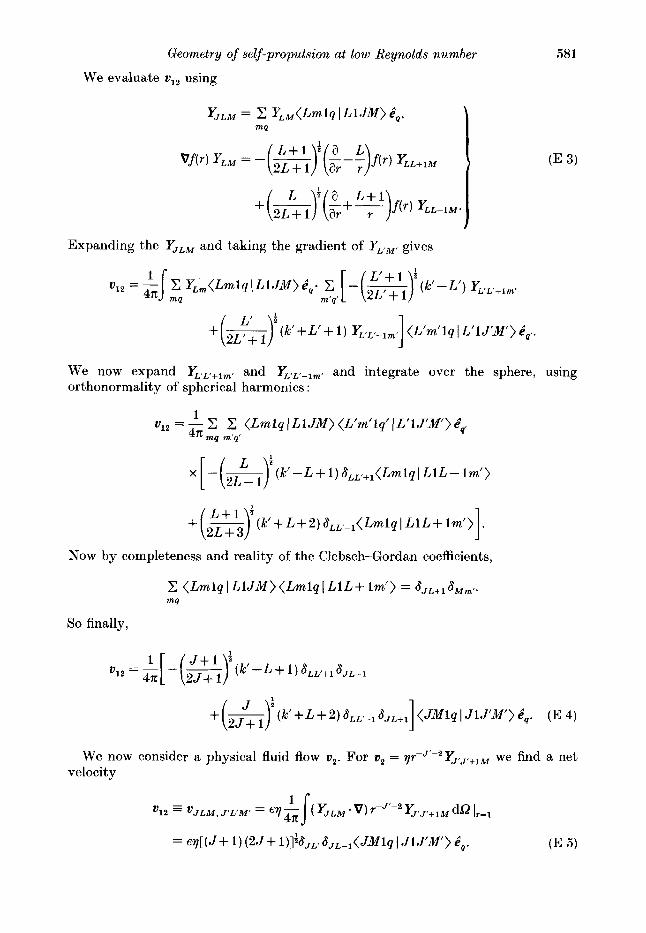
Appendix E. Calculation of F ( 9 ) In this Appendix, we sketch a derivation of (4.8) and compare it to a result of Blake
( 1 9 7 1 ~ ) . First, we compute the constant component v,, of the velocity field on the surface
of a sphere when the sphere is successively deformed by the (unphysical) fluid velocity fields v, = crk Y J L M and v, = Trk' Y J r L f M , :
Next, we consider physical fluid velocity fields (of the form given in (4.3)), whose values on the boundary of the two-sphere are vI = c YJLM and v, = 7 Y J T F M , , i.e.
cr-J-2 Y J j + l M
cr-J-l YJ J M
c Y J L M ( @ > $) = c y p J Y J J - i M I +c(&)?!I!(r-J-2- 2 -J ) y J J + l M (E 2 )
for r = 1. Using (E l), it is then straightforward to compute the net translation due to the closed cycle of shapes of figure 3, namely
d J L M , J'L'M' = C.m, J*L'M'ET.
Geometry of self-propulsion at low Reynolds number 58 1
We evaluate v,, using
Expanding the YJLM and taking the gradient of YLrM, gives
+(&)h+L'+ 1 ) q , 'L- lm' 1 (L'm'lqIL'lJ'M')e",,.
We now expand KrLflmf and YL,L'-lmr and integrate over the sphere, using orthonormality of spherical harmonics :
1 vl, = - C I; (Lmlql
471. mq m'q' L1 J M ) (L'm'lq' 1 L'WM') gq,
x - - [ ( 2;- l)t (k' - L + 1 ) 8,,,,(Lmlq I L 1L - lm))
1 + (sr (k' + L + 2 1 8LLr-l ( Lm 1 q I L 1 L + 1m' > .
Now by completeness and reality of the Clebsch-Gordan coefficients,
C (Lmlq I LlJM) (Lmlq I LlL+ lm' ) = 8JL+18Mm'. mq
So finally,
We now consider a physical fluid flow v,. For v, = yr-J'-2Y J,J'+IM we find a net velocity
582
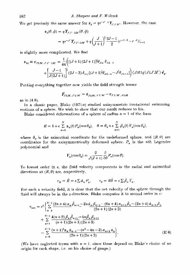
We get precisely the same answer for v 2 = r,w-J'-lY J , JfMr. However, the case
A . Shapere and F . Wilczek
v 2 ( B , $) = 7 yJ 'J - lM' (8 , $)
is slightly more complicated. We find
01, V J L M , j ' J ' - l M ' = [ ( J + 1)(2J+ l)]'fiJJL'fiJL-I
Putting everything together now yields the field strength tensor
- 4mt, J ' ~ M ' - v J L M , J ' L ' M ' - ~ J ' L ' M * , J L M
as in (4.8).
motions of a sphere. We wish to show that our result reduces to his. In a classic paper, Blake (1971 a ) studied axisymmetric irrotational swimming
Blake considered deformations of a sphere of radius a = 1 of the form
N N
R = l + e an(t)Pn(cos8,), f3 = O , + E C P,(t) V , ( O O S ~ , ) ,
where 0, is the azimuthal coordinate for the undeformed sphere, and (R,B) are coordinates for the axisymmetrically deformed sphere. Pn is the nth Legendre polynomial and
n=2 n=l
2 a J ( J + 1) ae Vn(c0sf3,) = ~ - P,(cos 0).
To lowest order in e, the fluid velocity components in the radial and azimuthal directions a t (B , 0) are, respectively,
v R = R = € C k n P n , v ~ = R B = E C P , V ~ ' , .
For such a velocity field, it is clear that the net velocity of the sphere through the fluid will always be in the z-direction. Blake computes it to second order in E :
N - 1 (n+ 1)2an k,,, - (n2-4n-2) L i n
( 2 n + l ) ( 2 n + 3 ) -z
n-2
(We have neglected terms with n = 1, since these depend on Blake's choice of an origin for each shape, i.e. on his choice of gauge.)
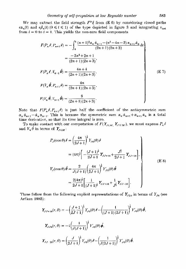
Geometry of self-propulsion at low Reynolds number 583
We may extract the field strength Ftr2 from (E 6) by considering closed paths ea,(t) and $,(t) (0 < t f 1) of the type depicted in figure 3 and integrating unet from t = 0 to t = 1 . This yields the non-zero field components
dt (n+ I)'an in+, - (n2 -4n-2) ci,
(2n+1)(2n+3) F(P, i , P,+l i ) = -
-2n2+2n+ 1 (2n+ 1)(2n+3)'
- -
4n (2n + 1) (2n + 3 ) '
8 ( 2 n + l ) ( 2 n + 3 ) '
B( v, 6, P,+l i ) =
F(V, e, v,,, 8) =
Note that F(P,i,F'n+li) is just half the coefficient of the antisymmetric sum a,a,+l-ci,a,+l. This is because the symmetric sum ~~,ci,+,+a,+~ci, is a total time derivative, so that its time integral is zero.
To m9ke contact with our computation of F ( Y J L M , Y J r C M , ) , we must express P, 4 and V, 8 in terms of YJLM :
These follow from the following explicit representations of U,,, in terms of Y,, (see Arf ken 1985) :
584
The last ingredients needed are four components of FJLM, J , L , M r [see (4.8)] :
A . Shapere and F . Wilczek
1 %+lo, J+1J+SO = “J + 1) (J + 2)14
1 4n &+lo, J+lJO = - (J +
1 w-1 47c W + 3 ’ c - 1 0 , J+IJ+PO = - [J(J + 2)li-
1 2 J - 1 FA-10, J + 1 J O = - - [J(J + 2 ) l i W . 47c
Here, we have made use of the Clebsch-Gordan coefficients
<J-101O(J-llJO) =
( J + 1010 IJ+ 11JO) =
We shall now compute F(P,r^,P,+,E) explicitly. Combining ( E 8) and (E 9), and using the linearity of F, we obtain
- - W + W + l - (W + 1) (W+3) ’
in agreement with (E 7). The remaining components of F may be evaluated similarly.
REFEREPU’CES ARFKEN, G. 1985 Mathematical Methods for Physicists. Academic. BATCHELOR, G . K. 1970 An Introduction to Fluid Dynamics. Cambridge University Press. BLAKE, J. R. 1971a A spherical envelope approach to ciliary propulsion. J . Fluid Mech. 46,
119-208. BLAKE, J. R. 1971 b Self propulsion due to oscillations on the surface of a cylinder at low Reynolds
BLAKE, J. R. & SLEIGH, M. A. 1975 Hydromechanical aspects of ciliary propulsion. In Swimming
BRENNEN, C. & WINET, H. 1977 Fluid mechanics of propulsion by cilia and flagella. A n n . Rev.
CHILDRESS, S. 1978 Mechanics of Swimming and Flying. Cambridge University Press. CHOQUET-BRUHAT, Y., DEWITT-MORRETTE, c. & DILLARD-BLEICK, M. 1977 Analysia, Manifolds,
EDMONDS, A. E. 1957 Angular Momentum in Quantum Mechanics. Princeton University Press.
number. Bull. Austral. Math. Soc. 3, 255-264.
and Flying in Nature (ed. T. Y. Wu, C. J. Brokaw and C. Brennen), pp. 185-210. Plenum.
Fluid Mech. 9, 339-398.
a d Topology. North-Holland.
Geometry of self-propulsion at low Reynolds number 585
EGUCHI. T.. CILKEY, P. B. & HANSEN, A. J. 1980 Gravitation, gauge theories, and differential
ENGLAND, H. 1971 Complex Variable Methods in Elasticity. Wiley-Interscience. HAPPEL, J. & BRENNRR, H. 1965 Low Reynolds Number Hydrodynamics. Prentice-Hall. HASIMOTO, H. & SANO, H. 1980 Stokeslets and eddies in creeping flow. Ann. Rev. Fluid Mech. 12,
HILL, R. & POWER, G. 1955 Extremum principles for slow viscous flow and the approximate
JAHN, T. L. & VOTTA, J . J . 1972 Locomotion of protozoa. A n n . Rev. Fluid Mech. 4, 93-116. KELLER, J. B. & RUBINOW, S. J. 1976 Swimming of flagellated microorganisms. Biophys. J . 16,
151. LAMB, H LIGHTHILL. J. 1952 On the squirming motion of nearly spherical deformable bodies through
LIGHTHILL, J. 1975 Mathematical Bio$uidmechanics. SIAM. MUSKHELISHVILI, N. I.
PEDLEY, T. J. (ed.) 1975 Scale Effects in Animal Locomotion. Academic. PURCELL, E. 1977 Life a t low Reynolds number. A n n . J . Phys. 45, 3. RAYLEIGH, LORD 1878 The Theory of Sound, vol. 1, chap. 19. Macmillan. RICHARDSON, S. 1968 Two-dimensional bubbles in slow viscous flows. J . Fluid Mech. 33,
4 7 w 9 3 . SHAPERE, A. & WILCZEK, F. 1988 Geometric Phases in Physics. World Scientific (to be
published). SHAPERE, A. & WILCZEK, F. 1989 Efficiencies of self-propulsion a t low Reynolds number.
J . Fluid Mech. 198, 587-599. SHENKER, S. 1986 Introduction to conformal and superconformal field theory. In Unijied 8tring
Thporirs (ed. D. Gross & M. Green). World Scientific. TAYLOR, GI. I . 1951 Analysis of the swimming of microscopic organisms. Proc. R . Soc. Lond. A209,
geometry. Phys. Rep. 66, 213.
335-364.
calculation of drag. &. J . Mech. Appl. Maths 9, 313-319.
1895 Hydrodynamics. Cambridge University Press.
liquids a t very small Reynolds number. Commun. Pure. Appl. Maths 5, 10!+118.
1953 Some Basic Problems of the Mathematicat Theory of Elasticity (translated by J. R. M. Radok). Noordhoff.
447-46 1.