Embed Size (px)
Citation preview
Elastic Tail Propulsionat Low Reynolds
Number
Tony S. Yu
BackgroundSwimming at LowReynolds Number
Dynamics of Elastic Tails
Fixed SwimmerExperiment
Propulsive Force
Tail Shape
Summary I
Free SwimmerExperiment
Swimming Velocity
Summary II
Elastic Tail Propulsion at Low Reynolds Number
An Experimental Study
Tony S. Yu
Advisor: Prof. A.E. Hosoi
Hatsopoulos Microfluids Laboratory
Department of Mechanical Engineering
Massachusetts Institute of Technology
Elastic Tail Propulsionat Low Reynolds
Number
Tony S. Yu
BackgroundSwimming at LowReynolds Number
Dynamics of Elastic Tails
Fixed SwimmerExperiment
Propulsive Force
Tail Shape
Summary I
Free SwimmerExperiment
Swimming Velocity
Summary II
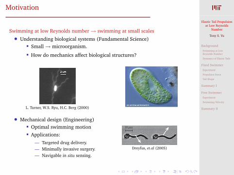
Motivation
Swimming at low Reynolds number → swimming at small scales
• Understanding biological systems (Fundamental Science)Small → microorganism.
How do mechanics affect biological structures?
L. Turner, W.S. Ryu, H.C. Berg (2000)
• Mechanical design (Engineering)Optimal swimming motion
Applications:
— Targeted drug delivery.— Minimally invasive surgery.— Navigable in situ sensing.
10 µm
Dreyfus, et.al (2005)
Elastic Tail Propulsionat Low Reynolds
Number
Tony S. Yu
BackgroundSwimming at LowReynolds Number
Dynamics of Elastic Tails
Fixed SwimmerExperiment
Propulsive Force
Tail Shape
Summary I
Free SwimmerExperiment
Swimming Velocity
Summary II
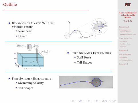
Outline
• DYNAMICS OF ELASTIC TAILS INVISCOUS FLUIDS
Nonlinear
Linearr(s)
t(s)
n(s)
y
x
ds
ψ(s)
D
BodyTail
StrainGauges
CantileverBeam
20 cm
35 cm 51 cm
VideoCamera
Robotic Swimmer
• FIXED SWIMMER EXPERIMENTS
Stall Force
Tail Shapes
• FREE SWIMMER EXPERIMENTS
Swimming Velocity
Tail Shapes
Elastic Tail Propulsionat Low Reynolds
Number
Tony S. Yu
BackgroundSwimming at LowReynolds Number
Dynamics of Elastic Tails
Fixed SwimmerExperiment
Propulsive Force
Tail Shape
Summary I
Free SwimmerExperiment
Swimming Velocity
Summary II
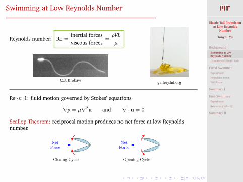
Swimming at Low Reynolds Number
Reynolds number: Re =inertial forcesviscous forces
=ρVLµ
C.J. Brokaw gallery.hd.org
Re 1: fluid motion governed by Stokes’ equations
∇p = µ∇2u and ∇ · u = 0
Scallop Theorem: reciprocal motion produces no net force at low Reynoldsnumber.
NetForce
NetForce
Closing Cycle Opening Cycle
Elastic Tail Propulsionat Low Reynolds
Number
Tony S. Yu
BackgroundSwimming at LowReynolds Number
Dynamics of Elastic Tails
Fixed SwimmerExperiment
Propulsive Force
Tail Shape
Summary I
Free SwimmerExperiment
Swimming Velocity
Summary II
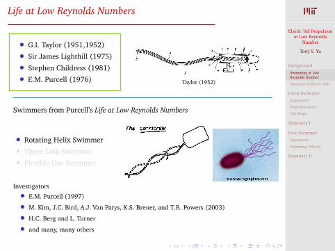
Life at Low Reynolds Numbers
• G.I. Taylor (1951,1952)
• Sir James Lighthill (1975)
• Stephen Childress (1981)
• E.M. Purcell (1976) Taylor (1952)
Swimmers from Purcell’s Life at Low Reynolds Numbers
• Rotating Helix Swimmer
• Three-Link Swimmer
• Flexible Oar Swimmer
Investigators
• E.M. Purcell (1997)
• M. Kim, J.C. Bird, A.J. Van Parys, K.S. Breuer, and T.R. Powers (2003)
• H.C. Berg and L. Turner
• and many, many others

Elastic Tail Propulsionat Low Reynolds
Number
Tony S. Yu
BackgroundSwimming at LowReynolds Number
Dynamics of Elastic Tails
Fixed SwimmerExperiment
Propulsive Force
Tail Shape
Summary I
Free SwimmerExperiment
Swimming Velocity
Summary II
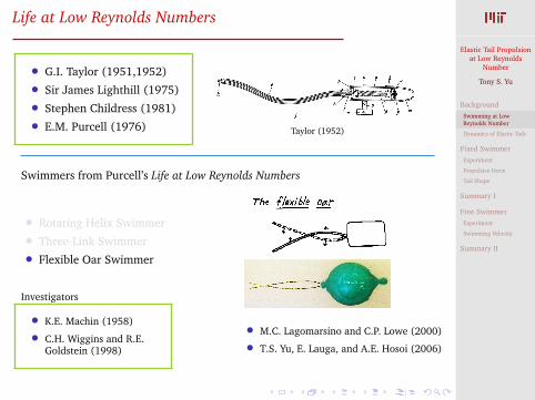
Life at Low Reynolds Numbers
• G.I. Taylor (1951,1952)
• Sir James Lighthill (1975)
• Stephen Childress (1981)
• E.M. Purcell (1976) Taylor (1952)
Swimmers from Purcell’s Life at Low Reynolds Numbers
• Rotating Helix Swimmer
• Three-Link Swimmer
• Flexible Oar Swimmer
Investigators
• L.E. Becker, S.A. Koehler, and H.A. Stone (2002)
• B. Chan and A.E. Hosoi
• D.S.W. Tam and A.E. Hosoi (2007)
Elastic Tail Propulsionat Low Reynolds
Number
Tony S. Yu
BackgroundSwimming at LowReynolds Number
Dynamics of Elastic Tails
Fixed SwimmerExperiment
Propulsive Force
Tail Shape
Summary I
Free SwimmerExperiment
Swimming Velocity
Summary II
Life at Low Reynolds Numbers
• G.I. Taylor (1951,1952)
• Sir James Lighthill (1975)
• Stephen Childress (1981)
• E.M. Purcell (1976) Taylor (1952)
Swimmers from Purcell’s Life at Low Reynolds Numbers
• Rotating Helix Swimmer
• Three-Link Swimmer
• Flexible Oar Swimmer
Investigators
• K.E. Machin (1958)
• C.H. Wiggins and R.E.Goldstein (1998)
• M.C. Lagomarsino and C.P. Lowe (2000)
• T.S. Yu, E. Lauga, and A.E. Hosoi (2006)
Elastic Tail Propulsionat Low Reynolds
Number
Tony S. Yu
BackgroundSwimming at LowReynolds Number
Dynamics of Elastic Tails
Fixed SwimmerExperiment
Propulsive Force
Tail Shape
Summary I
Free SwimmerExperiment
Swimming Velocity
Summary II
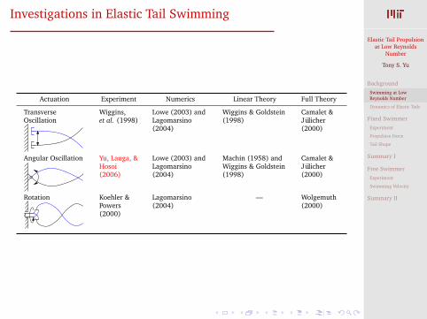
Investigations in Elastic Tail Swimming
Actuation Experiment Numerics Linear Theory Full Theory
TransverseOscillation
Wiggins,et al. (1998)
Lowe (2003) andLagomarsino(2004)
Wiggins & Goldstein(1998)
Camalet &Jülicher(2000)
Angular Oscillation Yu, Lauga, &Hosoi(2006)
Lowe (2003) andLagomarsino(2004)
Machin (1958) andWiggins & Goldstein(1998)
Camalet &Jülicher(2000)
Rotation Koehler &Powers(2000)
Lagomarsino(2004)
— Wolgemuth(2000)
Elastic Tail Propulsionat Low Reynolds
Number
Tony S. Yu
BackgroundSwimming at LowReynolds Number
Dynamics of Elastic Tails
Fixed SwimmerExperiment
Propulsive Force
Tail Shape
Summary I
Free SwimmerExperiment
Swimming Velocity
Summary II
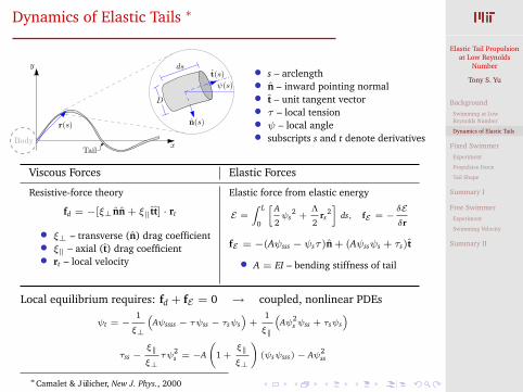
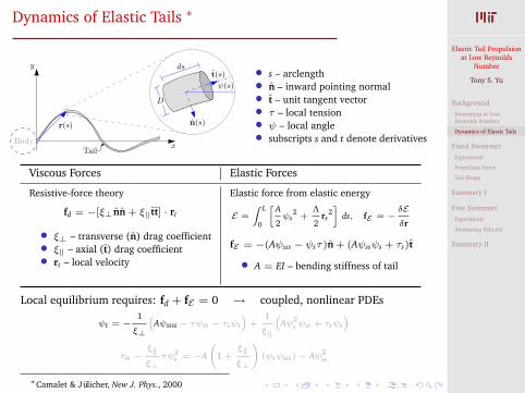
Dynamics of Elastic Tails ∗
r(s)
t(s)
n(s)
y
x
ds
ψ(s)
D
BodyTail
• s – arclength• n – inward pointing normal• t – unit tangent vector• τ – local tension• ψ – local angle• subscripts s and t denote derivatives
Viscous Forces Elastic Forces
Resistive-force theory
fd = −[ξ⊥nn + ξ‖ tt] · rt
• ξ⊥ – transverse (n) drag coefficient• ξ‖ – axial (t) drag coefficient• rt – local velocity
Elastic force from elastic energy
E =
Z L
0
» A
2ψs
2+
Λ
2rs
2–
ds, fE = −δEδr
fE = −(Aψsss − ψsτ)n + (Aψssψs + τs )t
• A = EI – bending stiffness of tail
Local equilibrium requires: fd + fE = 0 → coupled, nonlinear PDEs
ψt = −1
ξ⊥
“Aψssss − τψss − τsψs
”+
1
ξ‖
“Aψ2
s ψss + τsψs
”
τss −ξ‖
ξ⊥τψ
2s = −A
1 +
ξ‖
ξ⊥
!(ψsψsss)− Aψ2
ss
∗Camalet & Jülicher, New J. Phys., 2000
Elastic Tail Propulsionat Low Reynolds
Number
Tony S. Yu
BackgroundSwimming at LowReynolds Number
Dynamics of Elastic Tails
Fixed SwimmerExperiment
Propulsive Force
Tail Shape
Summary I
Free SwimmerExperiment
Swimming Velocity
Summary II
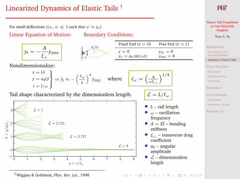
Linearized Dynamics of Elastic Tails †
For small deflections (i.e., ψ 1 such that ψ ≈ yx)
Linear Equation of Motion:
yt = −Aξ⊥
yxxxx
Boundary Conditions:
ω
a0Fixed End (x = 0) Free End (x = L)
y = 0 yxx = 0yx = a0 sin(ωt) yxxx = 0
Nondimensionalize:x = Lx
y = a0Ly
t = t/ω
9>>=>>;⇒ yt ≈ −„`ω
L
«4yxxxx where `ω =
“A
ωξ⊥
”1/4
Tail shape characterized by the dimensionless length: L = L/`ω
0 1 2 3 4 5 6 7 8 9−1
0
1
2
3 L = 1
L = 2.121
L = 3.737
L = 9
η = x/`ω
h=
y/a
0` ω
• L – tail length• ω – oscillation
frequency• A = EI – bending
stiffness• ξ⊥ – transverse drag
coefficient• a0 – angular
amplitude• L – dimensionless
length
†Wiggins & Goldstein, Phys. Rev. Let., 1998
Elastic Tail Propulsionat Low Reynolds
Number
Tony S. Yu
BackgroundSwimming at LowReynolds Number
Dynamics of Elastic Tails
Fixed SwimmerExperiment
Propulsive Force
Tail Shape
Summary I
Free SwimmerExperiment
Swimming Velocity
Summary II
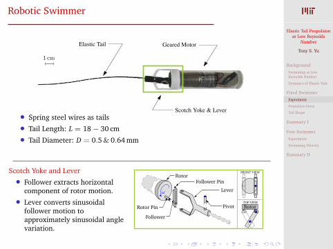
Robotic Swimmer
Elastic Tail
Scotch Yoke & Lever
Geared Motor
1 cm
• Spring steel wires as tails
• Tail Length: L = 18− 30 cm
• Tail Diameter: D = 0.5 & 0.64 mm
Scotch Yoke and Lever
• Follower extracts horizontalcomponent of rotor motion.
• Lever converts sinusoidalfollower motion toapproximately sinusoidal anglevariation.
FRONT VIEW
TOP VIEW
ω
Rotor
Follower
Lever
Pivot
Follower Pin
Rotor Pin Rotor
Elastic Tail Propulsionat Low Reynolds
Number
Tony S. Yu
BackgroundSwimming at LowReynolds Number
Dynamics of Elastic Tails
Fixed SwimmerExperiment
Propulsive Force
Tail Shape
Summary I
Free SwimmerExperiment
Swimming Velocity
Summary II
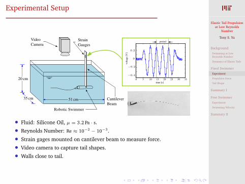
Experimental Setup
StrainGauges
CantileverBeam
20 cm
35 cm 51 cm
VideoCamera
Robotic Swimmer
0 5 10 15 20 25 30 35
−0.4
−0.2
0
0.2
time [s]
volta
ge[V
]
period
• Fluid: Silicone Oil, µ = 3.2 Pa · s.
• Reynolds Number: Re ≈ 10−2 − 10−3.
• Strain gages mounted on cantilever beam to measure force.
• Video camera to capture tail shapes.
• Walls close to tail.
Elastic Tail Propulsionat Low Reynolds
Number
Tony S. Yu
BackgroundSwimming at LowReynolds Number
Dynamics of Elastic Tails
Fixed SwimmerExperiment
Propulsive Force
Tail Shape
Summary I
Free SwimmerExperiment
Swimming Velocity
Summary II
Propulsive Force of Elastic Tail
0
0.2
0.4
0.6
0.8
Non
dim
ensi
onal
Forc
e,F
0 1 2 3 4 5
Nondimensional Length, L
linearnonlinear
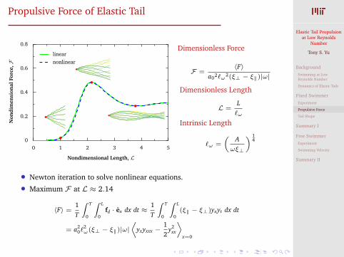
Dimensionless Force
F =〈F〉
a02`ω2(ξ⊥ − ξ‖)|ω|
Dimensionless Length
L =L`ω
Intrinsic Length
`ω =
„A
ωξ⊥
« 14
• Newton iteration to solve nonlinear equations.
• Maximum F at L ≈ 2.14
〈F〉 =1T
Z T
0
Z L
0fd · ex dx dt ≈
1T
Z T
0
Z L
0(ξ‖ − ξ⊥)yxyt dx dt
= a20`
2ω(ξ⊥ − ξ‖)|ω|
fiyxyxxx −
12
y2xx
flx=0
Elastic Tail Propulsionat Low Reynolds
Number
Tony S. Yu
BackgroundSwimming at LowReynolds Number
Dynamics of Elastic Tails
Fixed SwimmerExperiment
Propulsive Force
Tail Shape
Summary I
Free SwimmerExperiment
Swimming Velocity
Summary II
Propulsive Force of Elastic Tail
0
0.2
0.4
0.6
0.8
Non
dim
en
sion
al
Forc
e,F
Non
dim
en
sion
al
Forc
e,F
0 1 2 3 4 5
Nondimensional Length, LNondimensional Length, L
linear
nonlinear
L = 18 cm
L = 18 cm
L = 20 cm
L = 23 cm
L = 30 cm
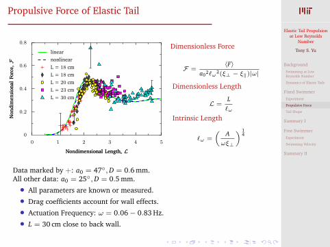
Dimensionless Force
F =〈F〉
a02`ω2(ξ⊥ − ξ‖)|ω|
Dimensionless Length
L =L`ω
Intrinsic Length
`ω =
„A
ωξ⊥
« 14
Data marked by +: a0 = 47,D = 0.6 mm.All other data: a0 = 25,D = 0.5 mm.
• All parameters are known or measured.
• Drag coefficients account for wall effects.
• Actuation Frequency: ω = 0.06− 0.83 Hz.
• L = 30 cm close to back wall.
Elastic Tail Propulsionat Low Reynolds
Number
Tony S. Yu
BackgroundSwimming at LowReynolds Number
Dynamics of Elastic Tails
Fixed SwimmerExperiment
Propulsive Force
Tail Shape
Summary I
Free SwimmerExperiment
Swimming Velocity
Summary II
Tail Shapes of Elastic Tail
(c)
(b)
(a)
−0.02
0
0.02−0.05
0
0.05
−0.05
0
0.05
y[m
]y
[m]
0 0.05 0.1 0.15 0.2
x [m]x [m]
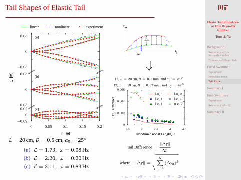
linear nonlinear experiment
L = 20 cm, D = 0.5 cm, a0 = 25
(a) L = 1.73, ω = 0.08 Hz
(b) L = 2.20, ω = 0.20 Hz
(c) L = 3.11, ω = 0.83 Hz
x
y
∆x
∆yn
⇓(1) L = 20 cm, D = 0.5 mm, and a0 = 25
(2) L = 18 cm, D = 0.63 mm, and a0 = 47
0
0.002
0.004
0.006
Tail
Dif
fere
nce
Tail
Dif
fere
nce
1.5 2 2.5 3 3.5
Nondimensional Length, LNondimensional Length, L
l-n, 1
l-e, 1
l-e, 1
l-n, 2
l-e, 2
n-e, 2
Tail Difference =‖∆y‖
NL
where ‖∆y‖ =
vuuut NXn=1
(∆yn)2
Elastic Tail Propulsionat Low Reynolds
Number
Tony S. Yu
BackgroundSwimming at LowReynolds Number
Dynamics of Elastic Tails
Fixed SwimmerExperiment
Propulsive Force
Tail Shape
Summary I
Free SwimmerExperiment
Swimming Velocity
Summary II
Conclusions
FIXED SWIMMER
• Oscillating, flexible tail generates propulsion at low Re.
• Linear theory describes tail motion and propulsive force well despite largeactuation angle (a0 = 47).
Tony S. Yu, Eric Lauga, and A.E. Hosoi, Phys. Fluids, (2006)
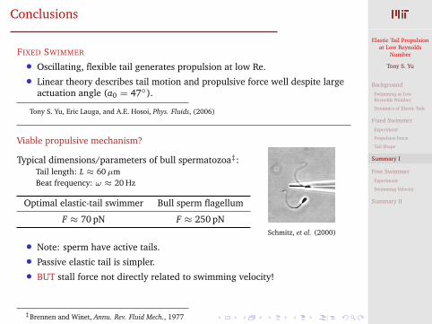
Viable propulsive mechanism?
Typical dimensions/parameters of bull spermatozoa‡:Tail length: L ≈ 60µmBeat frequency: ω ≈ 20 Hz
Optimal elastic-tail swimmer Bull sperm flagellum
F ≈ 70 pN F ≈ 250 pNSchmitz, et al. (2000)
• Note: sperm have active tails.
• Passive elastic tail is simpler.
• BUT stall force not directly related to swimming velocity!
‡Brennen and Winet, Annu. Rev. Fluid Mech., 1977
Elastic Tail Propulsionat Low Reynolds
Number
Tony S. Yu
BackgroundSwimming at LowReynolds Number
Dynamics of Elastic Tails
Fixed SwimmerExperiment
Propulsive Force
Tail Shape
Summary I
Free SwimmerExperiment
Swimming Velocity
Summary II
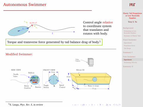
Autonomous Swimmer
ex
ey a0 sinωt
L
a
Control angle relativeto coordinate systemthat translates androtates with body.
Torque and transverse force generated by tail balance drag of body.§
Modified Swimmer:
SpeedControl
ToggleSwitch
Motor &Gearbox Battery
8 cmFRONT VIEWSIDE VIEW
BalloonNeedleValve
VideoCamera
Silicone Oil
Water (≈ 2 cm)
77 cm33 cm
12 cm
§E. Lauga, Phys. Rev. E, in review
Elastic Tail Propulsionat Low Reynolds
Number
Tony S. Yu
BackgroundSwimming at LowReynolds Number
Dynamics of Elastic Tails
Fixed SwimmerExperiment
Propulsive Force
Tail Shape
Summary I
Free SwimmerExperiment
Swimming Velocity
Summary II
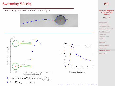
Swimming Velocity
Swimming captured and velocity analyzed:
0 0.5 1 1.5 2 2.5 3 3.5 40
1
2
3
4
5
6
×10−3
Nondimensional Length, L
Non
dim
ensi
onal
Vel
oci
ty,V
L = 2.64
L = 1.95
E. Lauga (in review)
• Dimensionless Velocity: V =〈U1〉
a02`ω|ω|
• L = 15 cm, a = 4 cm
Elastic Tail Propulsionat Low Reynolds
Number
Tony S. Yu
BackgroundSwimming at LowReynolds Number
Dynamics of Elastic Tails
Fixed SwimmerExperiment
Propulsive Force
Tail Shape
Summary I
Free SwimmerExperiment
Swimming Velocity
Summary II
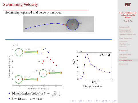
Swimming Velocity
Swimming captured and velocity analyzed:
0 0.5 1 1.5 2 2.5 3 3.5 40
1
2
3
4
5
6
×10−3
Nondimensional Length, L
Non
dim
ensi
onal
Vel
oci
ty,V
L = 2.64
L = 1.95
L = 3.55
E. Lauga (in review)
• Dimensionless Velocity: V =〈U1〉
a02`ω|ω|
• L = 15 cm, a = 4 cm
Elastic Tail Propulsionat Low Reynolds
Number
Tony S. Yu
BackgroundSwimming at LowReynolds Number
Dynamics of Elastic Tails
Fixed SwimmerExperiment
Propulsive Force
Tail Shape
Summary I
Free SwimmerExperiment
Swimming Velocity
Summary II
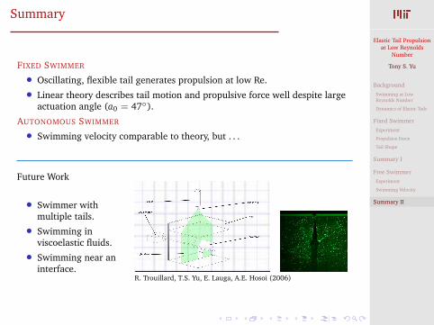
Summary
FIXED SWIMMER
• Oscillating, flexible tail generates propulsion at low Re.
• Linear theory describes tail motion and propulsive force well despite largeactuation angle (a0 = 47).
AUTONOMOUS SWIMMER
• Swimming velocity comparable to theory, but . . .
Future Work
• Swimmer withmultiple tails.
• Swimming inviscoelastic fluids.
• Swimming near aninterface.
R. Trouillard, T.S. Yu, E. Lauga, A.E. Hosoi (2006)
Elastic Tail Propulsionat Low Reynolds
Number
Tony S. Yu
Appendix
Hydrodynamic Drag
Wall Effects
Efficiency
Numerics
ExperimentalParameters
Free Swimmer Data
Force Measurement
Image Processing
Additional Slides
Hydrodynamic Drag
Wall Effects
Efficiency
Numerics
Experimental Parameters
Free Swimmer Data
Force Measurement
Image Processing
Elastic Tail Propulsionat Low Reynolds
Number
Tony S. Yu
Appendix
Hydrodynamic Drag
Wall Effects
Efficiency
Numerics
ExperimentalParameters
Free Swimmer Data
Force Measurement
Image Processing
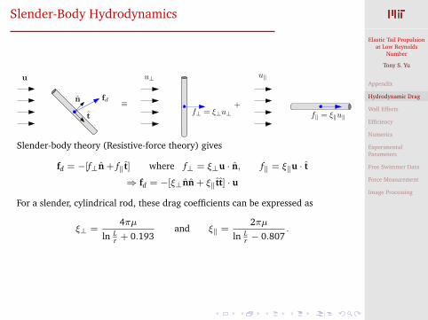
Slender-Body Hydrodynamics
u⊥ u‖
f⊥ = ξ⊥u⊥
u
fd
f‖ = ξ‖u‖
n
t
≡ +
Slender-body theory (Resistive-force theory) gives
fd = −[f⊥n + f‖ t] where f⊥ = ξ⊥u · n, f‖ = ξ‖u · t
⇒ fd = −[ξ⊥nn + ξ‖ tt] · u
For a slender, cylindrical rod, these drag coefficients can be expressed as
ξ⊥ =4πµ
ln Lr + 0.193
and ξ‖ =2πµ
ln Lr − 0.807
.
Elastic Tail Propulsionat Low Reynolds
Number
Tony S. Yu
Appendix
Hydrodynamic Drag
Wall Effects
Efficiency
Numerics
ExperimentalParameters
Free Swimmer Data
Force Measurement
Image Processing
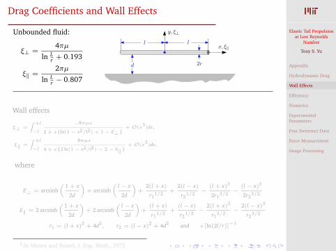
Drag Coefficients and Wall Effects
Unbounded fluid:
ξ⊥ =4πµ
ln Lr + 0.193
ξ‖ =2πµ
ln Lr − 0.807
x, ξ‖
y, ξ⊥
d
l l
2r
Wall effects
ξ⊥ =Z +l
−l
−8πµε
2 + εln(1 − x2/l2) + 1 − E⊥+ O(ε
3)dx,
ξ‖ =Z +l
−l
8πµε
4 + ε2 ln(1 − x2/l2) − 2 − E‖+ O(ε
3)dx,
where
E⊥ = arcsinh„ 1 + x
2d
«+ arcsinh
„ l − x
2d
«+
2(l + x)
r11/2
+2(l − x)
r21/2
−(l + x)3
2r13/2
−(l − x)3
2r23/2
E‖ = 2 arcsinh„ 1 + x
2d
«+ 2 arcsinh
„ l − x
2d
«+
(l + x)
r11/2
+(l − x)
r21/2
−2(l + x)3
r13/2
−2(l − x)3
r23/2
r1 = (l + x)2+ 4d2
, r2 = (l − x)2+ 4d2 and ε [ln(2l/r)]−1
§de Mestre and Russel, J. Eng. Math., 1975
Elastic Tail Propulsionat Low Reynolds
Number
Tony S. Yu
Appendix
Hydrodynamic Drag
Wall Effects
Efficiency
Numerics
ExperimentalParameters
Free Swimmer Data
Force Measurement
Image Processing
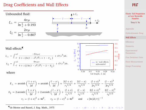
Drag Coefficients and Wall Effects
Unbounded fluid:
ξ⊥ =4πµ
ln Lr + 0.193
ξ‖ =2πµ
ln Lr − 0.807
x, ξ‖
y, ξ⊥
d
l l
2r
Wall effects¶
ξ⊥ =Z +l
−l
−8πµε
2 + εln(1 − x2/l2) + 1 − E⊥+ O(ε
3)dx,
ξ‖ =Z +l
−l
8πµε
4 + ε2 ln(1 − x2/l2) − 2 − E‖+ O(ε
3)dx,
where0
0.5
1
1.5
2
2.5
3
3.5
tail length, L [m]ξ ⊥
−ξ ‖
[Pa·
s]
0.16 0.2 0.24 0.28 0.320
0.1
0.2
0.3
0.4
0.6
erro
r
w/ wall effectsunbounded
0.5
E⊥ = arcsinh„ 1 + x
2d
«+ arcsinh
„ l − x
2d
«+
2(l + x)
r11/2
+2(l − x)
r21/2
−(l + x)3
2r13/2
−(l − x)3
2r23/2
E‖ = 2 arcsinh„ 1 + x
2d
«+ 2 arcsinh
„ l − x
2d
«+
(l + x)
r11/2
+(l − x)
r21/2
−2(l + x)3
r13/2
−2(l − x)3
r23/2
r1 = (l + x)2+ 4d2
, r2 = (l − x)2+ 4d2 and ε [ln(2l/r)]−1
¶de Mestre and Russel, J. Eng. Math., 1975
Elastic Tail Propulsionat Low Reynolds
Number
Tony S. Yu
Appendix
Hydrodynamic Drag
Wall Effects
Efficiency
Numerics
ExperimentalParameters
Free Swimmer Data
Force Measurement
Image Processing
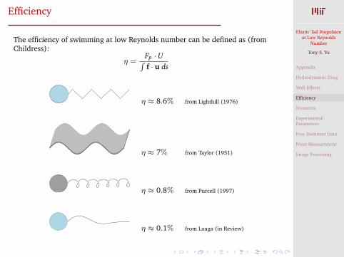
Efficiency
The efficiency of swimming at low Reynolds number can be defined as (fromChildress):
η =Fp · URf · u ds
η ≈ 8.6% from Lighthill (1976)
η ≈ 7% from Taylor (1951)
η ≈ 0.8% from Purcell (1997)
η ≈ 0.1% from Lauga (in Review)
Elastic Tail Propulsionat Low Reynolds
Number
Tony S. Yu
Appendix
Hydrodynamic Drag
Wall Effects
Efficiency
Numerics
ExperimentalParameters
Free Swimmer Data
Force Measurement
Image Processing
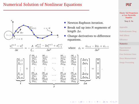
Numerical Solution of Nonlinear Equations
y
xBody
∆s
i = 0
i = Nψ(i)
• Newton-Raphson iteration.
• Break tail up into N segments oflength ∆s.
• Change derivatives to differenceequations.
ψn+1i − ψn
i
∆t= −
Aξ⊥
φn+1i+1 − 2φn+1
i + φn+1i−1
∆s2where φi =
ψi+1 − 2ψi + ψi−1
∆s2
2666664f1,1f2,1
...f1,Nf2,N
3777775| z
f
+
26666666664
∂f1,1∂ψ1
∂f1,1∂φ1
. . .∂f1,1∂ψN
∂f1,1∂φN
∂f2,1∂ψ1
∂f2,1∂φ1
. . .∂f2,1∂ψN
∂f2,1∂φN
......
. . ....
...∂f1,N∂ψ1
∂f1,N∂φ1
. . .∂f1,N∂ψN
∂f1,N∂φN
∂f2,N∂ψ1
∂f2,N∂φ1
. . .∂f2,N∂ψN
∂f2,N∂φN
37777777775| z
J
2666664∆ψ1∆φ1
...∆ψN∆φN
3777775| z
∆x
=
266666400...00
3777775 .
Elastic Tail Propulsionat Low Reynolds
Number
Tony S. Yu
Appendix
Hydrodynamic Drag
Wall Effects
Efficiency
Numerics
ExperimentalParameters
Free Swimmer Data
Force Measurement
Image Processing
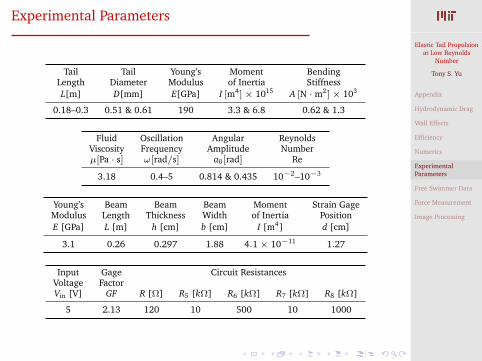
Experimental Parameters
Tail Tail Young’s Moment BendingLength Diameter Modulus of Inertia StiffnessL[m] D[mm] E[GPa] I [m4] × 1015 A [N · m2] × 103
0.18–0.3 0.51 & 0.61 190 3.3 & 6.8 0.62 & 1.3
Fluid Oscillation Angular ReynoldsViscosity Frequency Amplitude Numberµ[Pa · s] ω[rad/s] a0[rad] Re
3.18 0.4–5 0.814 & 0.435 10−2–10−3
Young’s Beam Beam Beam Moment Strain GageModulus Length Thickness Width of Inertia PositionE [GPa] L [m] h [cm] b [cm] I [m4] d [cm]
3.1 0.26 0.297 1.88 4.1 × 10⁻¹¹ 1.27
Input Gage Circuit ResistancesVoltage FactorVin [V] GF R [Ω] R5 [kΩ] R6 [kΩ] R7 [kΩ] R8 [kΩ]
5 2.13 120 10 500 10 1000
Elastic Tail Propulsionat Low Reynolds
Number
Tony S. Yu
Appendix
Hydrodynamic Drag
Wall Effects
Efficiency
Numerics
ExperimentalParameters
Free Swimmer Data
Force Measurement
Image Processing
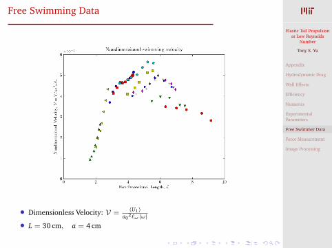
Free Swimming Data
• Dimensionless Velocity: V =〈U1〉
a02`ω|ω|
• L = 30 cm, a = 4 cm
Elastic Tail Propulsionat Low Reynolds
Number
Tony S. Yu
Appendix
Hydrodynamic Drag
Wall Effects
Efficiency
Numerics
ExperimentalParameters
Free Swimmer Data
Force Measurement
Image Processing
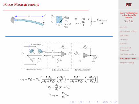
Force Measurement
FL
ε(y)x
yM
dx
h
NeutralAxis
M = −F (L− x)
σ = −My
I
ε =F (L− x)y
EI
R3
R5
Vin
Strain Gages
−+
−+
R4
Wheatstone Bridge Differential Amplifier Inverting Amplifier
R1
R2
V1
V2
V3
VDAQ
R5
R6
R6
R7
R8
(V1 − V2) = Vin
»R1R2
(R1 + R2)2
„dR1
R1
«+
R3R4
(R3 + R4)2
„−
dR3
R3
«–V3 =
R6
R5(V1 − V2)
VDAQ = −R8
R7V3.
Elastic Tail Propulsionat Low Reynolds
Number
Tony S. Yu
Appendix
Hydrodynamic Drag
Wall Effects
Efficiency
Numerics
ExperimentalParameters
Free Swimmer Data
Force Measurement
Image Processing
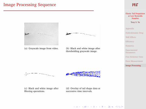
Image Processing Sequence
(a) Grayscale image from video. (b) Black and white image afterthresholding grayscale image.
(c) Black and white image afterfiltering operations.
(d) Overlay of tail shape data atsuccessive time intervals.
Elastic Tail Propulsionat Low Reynolds
Number
Tony S. Yu
Appendix
Hydrodynamic Drag
Wall Effects
Efficiency
Numerics
ExperimentalParameters
Free Swimmer Data
Force Measurement
Image Processing
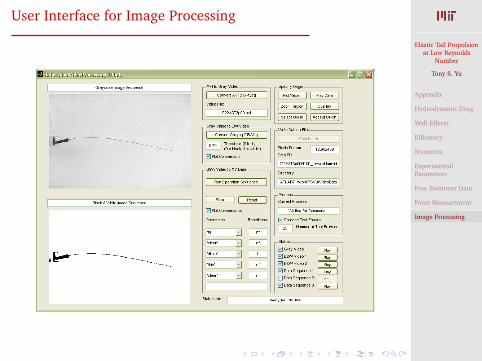
User Interface for Image Processing