Geometry in CT Reconstruction

Copyright 2011 Benjamin Kimia

February 22, 2011

Contents

1 Introduction to CT Reconstruction 31.1 Linear Attenuation Coefficient . . . . . . . . . . . . . . . . . . 31.2 Linear Tomography . . . . . . . . . . . . . . . . . . . . . . . . 51.3 Radon Transform . . . . . . . . . . . . . . . . . . . . . . . . . 61.4 Understanding Back Projection . . . . . . . . . . . . . . . . . 81.5 The Fourier Approach to CT Reconstruction . . . . . . . . . . 121.6 Filtered Backprojection . . . . . . . . . . . . . . . . . . . . . . 121.7 Watch out for those singularities: A review of Calculus . . . . 171.8 The Spatial Domain Approach to CT Reconstruction . . . . . 181.9 Inverse Radon Transform . . . . . . . . . . . . . . . . . . . . . 20

2 Fan Beam Geometry 212.1 Radon Transform and Fan Beam Geometry . . . . . . . . . . . 242.2 Radon Inversion Formula for Fan Beam Geometry . . . . . . . 262.3 Convolution in Fan Beam Geometry . . . . . . . . . . . . . . . 30

3 Flirting with Filtering 323.1 Introduction . . . . . . . . . . . . . . . . . . . . . . . . . . . . 323.2 Filtering . . . . . . . . . . . . . . . . . . . . . . . . . . . . . . 323.3 Matched Filtering . . . . . . . . . . . . . . . . . . . . . . . . . 363.4 Detecting Spots . . . . . . . . . . . . . . . . . . . . . . . . . . 37

3.4.1 Detecting A Gaussian Spot . . . . . . . . . . . . . . . 373.4.2 Detecting A Circular Spot . . . . . . . . . . . . . . . . 38

4 Taylor Expansion in the View Space 41

5 Geometric Tomography 415.1 Fan Beam Geometry . . . . . . . . . . . . . . . . . . . . . . . 46

1

6 Cone Beam Tomography and Volumetric CT 486.1 Notation and Definition . . . . . . . . . . . . . . . . . . . . . 506.2 Relating Cone Beam and Radon Transform . . . . . . . . . . . 546.3 Reconstruction Algorithms for Cone Beam Helical CT . . . . . 576.4 History of Helical Cone Beam CT Development . . . . . . . . 636.5 Material to be worked into this section . . . . . . . . . . . . . 646.6 Numerical algorithms for helical cone-beam reconstruction . . 65

7 Radon’s Proof 66

8 To Do 67

A Integrals Involving Gaussians and Derivatives of Gaussians 71A.1 Integrals involving a Gaussian and its derivatives . . . . . . . 71A.2 Fourier Transform of the Gaussian . . . . . . . . . . . . . . . . 72A.3 Integrals of the Gabor Filter . . . . . . . . . . . . . . . . . . . 73A.4 . . . . . . . . . . . . . . . . . . . . . . . . . . . . . . . . . . . 74

B Integrals Involving Characteristic Function of Circular Do-mains 77B.1 . . . . . . . . . . . . . . . . . . . . . . . . . . . . . . . . . . . 77B.2 . . . . . . . . . . . . . . . . . . . . . . . . . . . . . . . . . . . 78

C Some Standard Fourier Formulas 79

D A Numerically stable method to find an extremum 80

E Solving A sin θ +B cos θ = C 81

F Π-line membership 83F.1 References not included in the paper yet . . . . . . . . . . . . 88

2

1 Introduction to CT Reconstruction

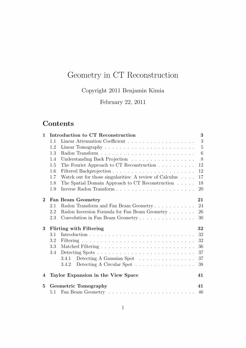
The key to CT reconstruction is a characterization of how X-rays are ab-sorbed by material. Since X-rays are electromagnetic waves, we considerhow the latter are absorbed as a function of the properties of the materialthrough which the light is traveling, as studied in the field of optics. Thisabsorption is governed by the Beer Lambert law, also alternatively knownas the Beer’s law or the Lambert Beer law or the Beer-Lambert-Bouguer,Figure xx. In short, this law states that the intensity of light passed througha slab of length l drops exponentially with l, i.e.,

I(l) = I0 e−αl, (1)

where I0 is the original intensity of the light, etc...

Figure 1: An illustration of the BeerLambert law in optics

1.1 Linear Attenuation Coefficient

Consider an X-ray beam going through some material. The probability thata photon gets removed from a beam (either absorbed or scattered) dependson (i) the energy of the photon, and (ii) the nature of the material throughwhich the beam passes. Define the linear attenuation coefficient µte of tissuet at energy e as

µte = − ln(pe), (2)

where pe is the probability that a photon of energy e transmits through auniform slab of unit length of tissue t in a direction perpendicular to the faceof the slab. For example, the linear attenuation coefficient of water at 73 kevis 0.19 cm−1.

3

A general model of X-ray absorption is based on an independence as-sumption: The extent of X-ray absorption by the material by any portionof space is independent of that corresponding to the complementary space.This independence is essentially what gives rise to the exponential decay inX-ray intensity. The following discussion is adapted from [11]. Specifically,consider a slab of non-uniform material and denote the linear attenuation co-efficient as a function of the coordinate x along the space as µe(x). Let pe(x)be the probability of absorption in a slab of width dx at x, i.e., the proba-bility that a photon of energy e is transmitted as far as x. Note that pe(x)is a monotonically decreasing function of x. Now, consider an infinitesimalsection dx of the slab from x to x+ dx. Let qe(x, dx) denote the probabilitythat a photon of energy e which has reached x will not be transmitted be-yond x+ dx. It is clear, therefore, that the probability of a photon reachingx+ dx is the probability of it reaching x and being transmitted through thedx slab:

pe(x+ dx) = pe(x)(1− qe(x, dx)),

or

qe(x, dx) = −pe(x+ dx)− pe(x)

pe(x).

Now let

µe(x) = limdx→0

qe(x, dx)

dx= −p

′e(x)

pe(x)= −d(ln(pe(x))

dx.

Observe that∫ A

0

µe(x)dx = −∫ A

0

−d(ln(pe(x))

dxdx = − ln(pe(x))|A0 = − ln(pe(A))+ln(1) = − ln(pe(A)).

Now, for a uniform slab of unit length, i.e. where µe(x) = µe and A = 1, wehave

µe =

∫ 1

0

µe(x)dx = − ln(pe(1)).

Comparing this to Equation(2), it is clear that µe = µte. Since qe as aprobability is dimensionless, µe has dimension of length−1 and so does µte.

In actual practice, since calibration is required to make measurements uni-form across detection, the actual linear attenuation coefficient µte is measuredrelative to µce, the linear attenuation coefficient of the calibration material.Define the relative linear attenuation coefficient as

µt,ae = µte − µae .

4

Note that line integrals of these quantities are simply related:∫ A

0

µt,ae (x)dx =

∫ A

0

(µte(x)− µae(x))dx

=

∫ A

0

µte(x)dx−∫ A

0

µae(x)dx

= − ln(pte(A)) + ln(pae(A))

= − ln(pte(A)

pae(A)).

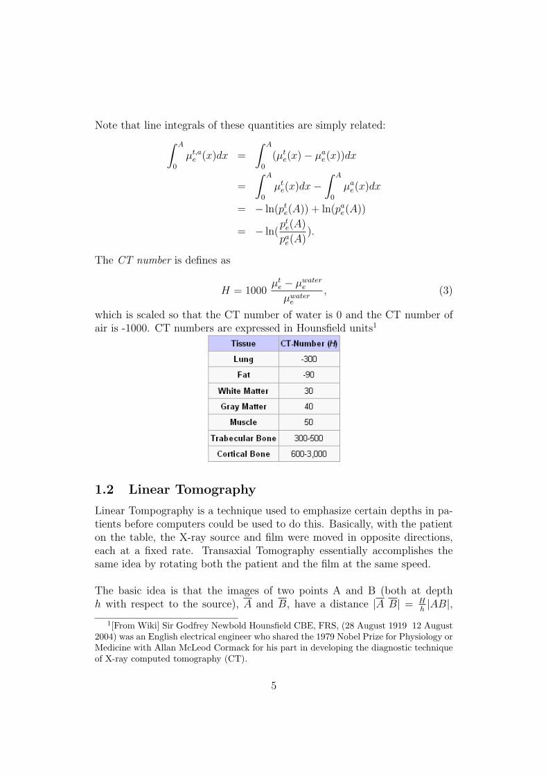
The CT number is defines as

H = 1000µte − µwatere

µwatere

, (3)

which is scaled so that the CT number of water is 0 and the CT number ofair is -1000. CT numbers are expressed in Hounsfield units1

1.2 Linear Tomography

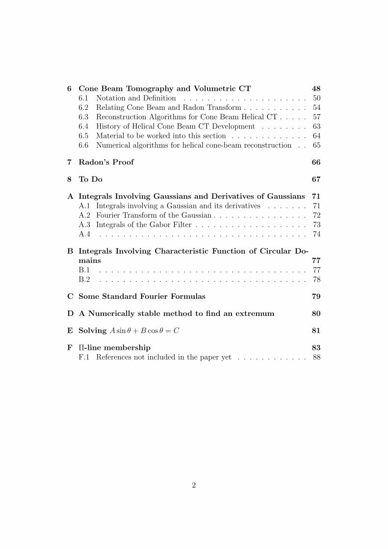
Linear Tompography is a technique used to emphasize certain depths in pa-tients before computers could be used to do this. Basically, with the patienton the table, the X-ray source and film were moved in opposite directions,each at a fixed rate. Transaxial Tomography essentially accomplishes thesame idea by rotating both the patient and the film at the same speed.

The basic idea is that the images of two points A and B (both at depthh with respect to the source), A and B, have a distance |A B| = H

h|AB|,

1[From Wiki] Sir Godfrey Newbold Hounsfield CBE, FRS, (28 August 1919 12 August2004) was an English electrical engineer who shared the 1979 Nobel Prize for Physiology orMedicine with Allan McLeod Cormack for his part in developing the diagnostic techniqueof X-ray computed tomography (CT).

5

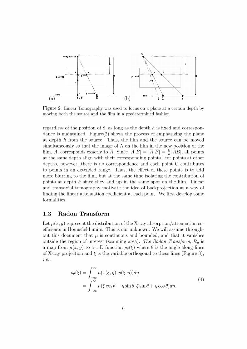
(a) (b)

Figure 2: Linear Tomography was used to focus on a plane at a certain depth bymoving both the source and the film in a predetermined fashion

regardless of the position of S, as long as the depth h is fixed and correspon-dance is maintained. Figure(2) shows the process of emphasizing the planeat depth h from the source. Thus, the film and the source can be movedsimultaneously so that the image of A on the film in the new position of thefilm, A, corresponds exactly to A. Since |A B| = |A B| = H

h|AB|, all points

at the same depth align with their corresponding points. For points at otherdepths, however, there is no correspondence and each point C contributesto points in an extended range. Thus, the effect of these points is to addmore blurring to the film, but at the same time isolating the contribution ofpoints at depth h since they add up in the same spot on the film. Linearand transaxial tomography motivate the idea of backprojection as a way offinding the linear attenuation coefficient at each point. We first develop someformalities.

1.3 Radon Transform

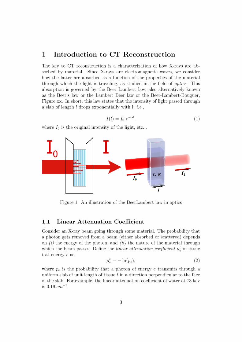
Let µ(x, y) represent the distribution of the X-ray absorption/attenuation co-efficients in Hounsfield units. This is our unknown. We will assume through-out this document that µ is continuous and bounded, and that it vanishesoutside the region of interest (scanning area). The Radon Transform, Rµ isa map from µ(x, y) to a 1-D function ρθ(ξ) where θ is the angle along linesof X-ray projection and ξ is the variable orthogonal to these lines (Figure 3),i.e.,

ρθ(ξ) =

∫ ∞−∞

µ(x(ξ, η), y(ξ, η))dη

=

∫ ∞−∞

µ(ξ cos θ − η sin θ, ξ sin θ + η cos θ)dη.

(4)

6

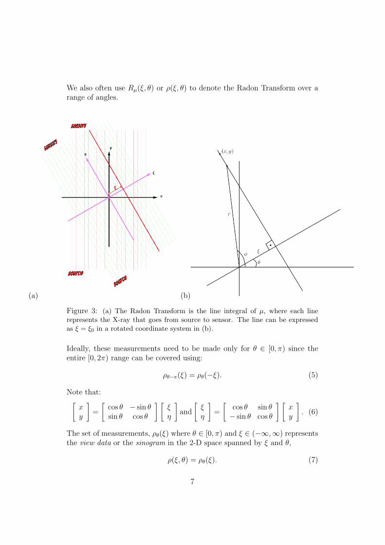
We also often use Rµ(ξ, θ) or ρ(ξ, θ) to denote the Radon Transform over arange of angles.

(a) (b)

Figure 3: (a) The Radon Transform is the line integral of µ, where each linerepresents the X-ray that goes from source to sensor. The line can be expressedas ξ = ξ0 in a rotated coordinate system in (b).

Ideally, these measurements need to be made only for θ ∈ [0, π) since theentire [0, 2π) range can be covered using:

ρθ−π(ξ) = ρθ(−ξ). (5)

Note that:[xy

]=

[cos θ − sin θsin θ cos θ

] [ξη

]and

[ξη

]=

[cos θ sin θ− sin θ cos θ

] [xy

]. (6)

The set of measurements, ρθ(ξ) where θ ∈ [0, π) and ξ ∈ (−∞,∞) representsthe view data or the sinogram in the 2-D space spanned by ξ and θ,

ρ(ξ, θ) = ρθ(ξ). (7)

7

Our goal is to recover µ(x, y) from ρ(ξ, θ).

Remark: The Radon Transform is integration along a line. We can specifya line by its distance ξ from the origin and the angle it makes with the x-axisθ. A point (x, y) is on the line if and only if (x, y).(cos θ, sin θ) = ξ. Thus ina 2D plane δ(x cos θ+ y sin θ− ξ) is non-zero only when the point (x, y) is onthis line. Thus, we see the Radon Transform.

Alternatively, in polar notation, a point (r, φ) is on the line if and only if(r cosφ, r sinφ)(cos θ, sin θ) = ξ which reduces to r cos(φ−θ) = ξ. This givesan expression for the Radon Transform in polar notation

ρ(ξ, θ) =

∫ π

0

∫ ∞−∞

µ(r, φ)δ(r cos(φ− θ)− ξ)rdrdφ

also written as

ρ(ξ, θ) =

∫ ∞−∞

∫ ∞−∞

µ(x, y)δ(x cos θ + y sin θ − ξ)dxdy.

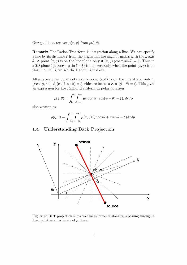
1.4 Understanding Back Projection

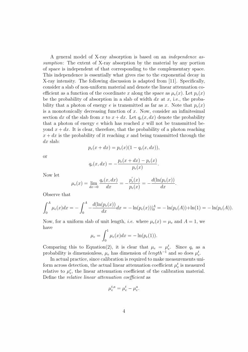
Figure 4: Back projection sums over measurements along rays passing through afixed point as an estimate of µ there.

8

The idea of backprojection goes back to Linear and Transaxial Tomography.Consider the same idea with a single source and a single sensor rotatingaround the object around some fixed point ρ(x0, y0), Figure(4). The idea isto backproject each view data to all points giving rise to it in an accumulativefashion,i.e., the estimated linear attenuation coefficient at each point in thesum of intensities measured for all rays going through the point. The sensorreading for each ray through ρ, indexed by θ, is obtained from Equation (4)

ρ(ξ0, θ) =

∫ ∞−∞

µ(ξ0 cos θ − η sin θ, ξ0 sin θ + η cos θ)dη, (8)

where ξ0 = x0 cos θ + y0 sin θ. Each ray passes through ρ, but any otherpoint participates in the view data in only one ray. Thus, in the cumulativeresponse, the contribution of all points fades in comparison to that of ρ. Theprocess of accumulating all ray measurements through ρ and using it as anestimate of µ(x0, y0) at ρ is called backprojection. Formally,

µBP (x0, y0) =1

π

∫ π

0

ρ(ξ0, θ)dθ, where ξ0 = x0 cos θ + y0 sin θ. (9)

How good an estimate of µ is µBP ? The following theorem relates thebackprojection estimate of µ to µ.

Theorem 1.

µBP (x, y) = µ(x, y) ∗ 1

π

1√x2 + y2

. (10)

Proof. We can relate the two by simplifying Equation (9) using Equation(8):

µBP (x0, y0) =1

π

∫ π

0

[∫ ∞−∞

µ(ξ0(θ) cos θ − η sin θ, ξ0(θ) sin θ + η cos θ) dη

]dθ,

(11)where ξ0(θ) = x0 cos θ+y0 sin θ. We can gain a better insight into this integralby switching to a polar coordinate system centered around (x0, y0),

x = x0 + r cosφ

y = y0 + r sinφ.(12)

Now, given (θ, η) in integral (11), these identify (x, y)x = ξ0(θ) cos θ − η sin θ

y = ξ0(θ) sin θ + η cos θ.(13)

9

Equating (12) and (13) relates (r,φ) to (η, θ):r cosφ = ξ0(θ) cos θ − η sin θ − x0 = (ξ0(θ) cos θ − η sin θ)− (ξ0(θ) cos θ − η0(θ) sin θ)

r sinφ = ξ0(θ) sin θ + η cos θ − y0 = (ξ0(θ) sin θ + η cos θ)− (ξ0(θ) sin θ + η0(θ) cos θ)

or, r cosφ = −(η − η0(θ)) sin θ

r sinφ = (η − η0(θ)) cos θ

where ξ0(θ) = x0 cos θ + y0 sin θ

η0(θ) = −x0 sin θ + y0 cos θ.

When η < η0(θ), we have r = −(η − η0(θ))

φ = θ − π

2

or, solving for (η, θ) η = −r − x0 cosφ− y0 sinφ

θ = φ+ π/2.

When η > η0(θ), we have r = η − η0(θ)

φ = θ +π

2

or, solving for (η, θ) η = r + x0 cosφ+ y0 sinφ

θ = φ− π/2.

In rewriting (9) in terms of r and φ, we will also need an expression for ξ0(θ).When η < η0(θ)

ξ0(θ) = x0 cos(φ+π

2) + y0 sin(φ+

π

2)

= −x0 sinφ+ y0 cosφ.

10

and when η > η0(θ)

ξ0(θ) = x0 cos(φ− π

2) + y0 sin(φ− π

2)

= x0 sinφ− y0 cosφ.

We can now rewrite µBP in (9) as

µBP (x0, y0) =1

π

∫ π

0

∫ η0(θ)

−∞µ(ξ0(θ) cos θ − η sin θ, ξ0(θ) sin θ + η cos θ) dηdθ

+1

π

∫ π

0

∫ ∞η0(θ)

µ(ξ0(θ) cos θ − η sin θ, ξ0(θ) sin θ + η cos θ) dηdθ

=1

π

∫ π2

−π2

∫ 0

−∞µ((−x0 sinφ+ y0 cosφ)(− sinφ)− (−r − x0 cosφ− y0 sinφ)(cosφ),

(−x0 sinφ+ y0 cosφ)(cosφ) + (−r − x0 cosφ− y0 sinφ)(− sinφ)) drdφ

+1

π

∫ 3π2

π2

∫ ∞0

µ((x0 sinφ− y0 cosφ)(sinφ)− (r + x0 cosφ+ y0 sinφ)(− cosφ),

(x0 sinφ− y0 cosφ)(− cosφ) + (r + x0 cosφ+ y0 sinφ)(sinφ)) drdφ

=1

π

∫ π2

−π2

∫ ∞0

µ((x0 sinφ− y0 cosφ) sinφ+ (x0 cosφ+ y0 sinφ) cosφ+ r cosφ,

(−x0 sinφ+ y0 cosφ) cosφ+ (x0 cosφ+ y0 sinφ) sinφ+ r sinφ) drdφ

+1

π

∫ 3π2

π2

∫ ∞0

µ((x0 sinφ− y0 cosφ) sinφ+ (x0 cosφ+ y0 sinφ) cosφ+ r cosφ,

(−x0 sinφ+ y0 cosφ) cosφ+ (x0 cosφ+ y0 sinφ) sinφ+ r sinφ) drdφ

=1

π

∫ 2π

0

∫ ∞0

µ(x0 + r cosφ, y0 + r sinφ)drdφ.

We are now in a position to interpret this as an area integral, i.e.

µBP (x0, y0) =1

π

∫ 2π

0

∫ ∞0

[µ(x0 + r cosφ, y0 + r sinφ)

r

]rdrdφ

=1

π

∫ ∞−∞

∫ ∞−∞

µ(x, y)√(x− x0)2 + (y − y0)2

dxdy

= µ(x, y) ∗ 1

π

1√x2 + y2

x=x0,y=y0

,

which is the 1r

filter well-known from the Fourier approach to the CT recon-struction. In summary, the back projection process gives a blurred estimateof µ(x, y) with a 1

rblurring filter.

11

1.5 The Fourier Approach to CT Reconstruction

In this approach, the CT-reconstruction of µ(x, y) relies on its Fourier Trans-form,

µ(ωx, ωy) = Fµ(x, y) =

∫ ∞−∞

∫ ∞−∞

µ(x, y)e−iωxxe−iωyydxdy.

Consider a polar representation of µ in the Fourier domain, i.e., µ(ω, θ),where ωx = ω cos θ and ωy = ω sin θ. We have

µ(ω, θ) =

∫ ∞−∞

∫ ∞−∞

µ(x, y)e−i(ω cos θ)xe−i(ω sin θ)ydxdy

=

∫ ∞−∞

∫ ∞−∞

µ(x, y)e−i(x cos θ+y sin θ)ωdxdy

=

∫ ∞−∞

∫ ∞−∞

µ(ξ cos θ − η sin θ, ξ sin θ + η cos θ)e−iξωdξdη.

The latter integral can be viewed in the form of a 1-D Fourier Transformwhere θ is fixed, but ω is varying:

µ(ω, θ) =

∫ ∞−∞

[∫ ∞−∞

µ(ξ cos θ − η sin θ, ξ sin θ + η cos θ)dη

]e−iξωdξ

=

∫ ∞−∞

ρ(ξ, θ)e−iξωdξ

= Fξρ(ξ, θ)(ω) = ρ(ω, θ),

where ρ(ω, θ) is the one dimensional Fourier Transform of ρ(ω, θ) for fixedθ along the variable ξ. In other words, when keeping θ fixed in the Fourierdomain, this slice of the Fourier Transform of µ(ω, θ) corresponds exactly tothe 1-D Fourier Transform of the Radon Transform for that θ, i.e., ρθ(ξ).This is the central slice theorem. Alternatively, replacing each column ofthe sinogram by its Fourier Transform gives the Fourier Transform of µ inpolar coordinates.

Need some figures

1.6 Filtered Backprojection

The central slice theorem allows us to recover µ(x, y) from the measurementsusing the inverse Fourier Transform and a change of coordinates from the

12

Cartesian coordinates (ωx, ωy) to the polar coordinates ω, θ.

µ(x, y) =1

4π2

∫ ∞−∞

∫ ∞−∞

µ(ωx, ωy)eiωxxeiωyydωxdωy

=1

4π2

∫ π

0

∫ ∞−∞

µ(ω, θ)eiω(cos θ)xeiω(sin θ)y|ω|dωdθ

=1

2π

∫ π

0

[1

2π

∫ ∞−∞

µ(ω, θ) |ω| eiω(x cos θ+y sin θ)dω

]dθ. (14)

The inner integral in the square brackets is the one-dimensional inverseFourier Transform of µ(ω, θ)|ω| along the variable ω with fixed θ. Define

ρ∗(ξ, θ) = F−1[µ(ω, θ)|ω|] =1

2π

∫ ∞−∞

µ(ω, θ) |ω| eiω(x cos θ+y sin θ)dω. (15)

Then

µ(x, y) =1

2π

∫ π

0

ρ∗θ(x cos θ + y sin θ)dθ. (16)

Equation (16) provided the recipe for recovery of µ:

1)Filtering step: From ρ(ξ, θ), find ρ∗(ξ, θ) = F−1ω Fξρ(ξ, θ)|ω|,

2)Backprojection: Sum over ρ∗(ξ, θ) over all θ.The first step is called the filtering step because it seems to be inter-

pretable as a convolution: Observing that a product in the Fourier domainis a convolution in the spatial domain it is tempting to write

ρ∗(ξ, θ) = ρ(ξ, θ) ∗ F−1|ω|. (17)

However, the function |ω| has infinite energy and such a split into two func-tions is not valid. A different split is possible:

F−1ω Fξρ(ξ, θ)|ω| = F−1

ω Fξρ(ξ, θ)H(w)

.H(w)|ω| (18)

= F−1ω Fξρ(ξ, θ)H(w)

∗ F−1ω H(w)|ω|, (19)

where H(ω) is expected to decrease sufficiently fast to compensate for theincrease by |ω| so that F−1

ω H(w)|ω| exists. If ρ(ξ, θ) is band-limited sothat frequencies beyond Ω are not present,

Fξρ(ξ, θ) = 0 when ω > Ω, (20)

then we can design H(ω) to be 1 up to Ω, and then drop monotonically tozero.

13

H(ω) = 1, |ω| ≤ ΩH(ω) 6= 0, otherwise.

(21)

In this case we have we have

F−1ω Fξρ(ξ, θ)H(w)

= F−1ω Fξρ(ξ, θ)

1 = ρ(ξ, θ), (22)

andρ∗(ξ, θ) = ρ(ξ, θ) ∗ F−1

ω H(w)|ω|. (23)

The filter H(ω) can be designed a number of ways. First, the filter definedby Ramachandran and Lakshiminarayanan [23], known now as the Ram-Lak filter, is simply obtained by limiting the frequency domain response,Figure(5).

H(ω) =

1, |ω ≤ Ω0, otherwise.

(24)

so that the overall filter is HRL(ω) = HRL(ω)|ω|, or,

HRL(ω) =

|ω|, |ω| ≤ Ω0, otherwise.

(25)

Using Appendix(C), Formula 3, the spatial domain filter is

hRL(x) =Ω2

π[sinc(Ωx)− 1

2sinc2(

Ωx

2)], (26)

See Figure(5).Second, the Shepp-Logan filter [25] has a similar design that it also limits

the frequency upper bound, but in contrast to the Ram-Lak filter, it does sogradually using a sinc function 2Ω

πsinc(πω

2Ω), Figure(5), with the overall filter

defined as

HSL(ω) =

∣∣sin (πω2Ω

)∣∣ , |ω| < Ω0, otherwise

(27)

14

(a) (b)

Figure 5: (a)Examples of the band-limited filter function of sampled data. Notethe cyclic repetitiveness of the digital filter. (b) Spatial domain filter kernels cor-responding to the filter functions shown in the Ram-Lak filter is a high-pass filterwith a sharp response but results in some noise enhancement, while the Shepp-Logan and the Hamming window filters are noise-smoothed filters and thereforehave better SNR. (Images taken from [3])

The spatial filter corresponding to the Shepp-Logan filter is

hSL(ω) =1

2π

∫ ∞−∞

HSL(ω)eiωxdω

=1

2π

∫ Ω

−Ω

∣∣∣sin(πω2Ω

)∣∣∣ eiωxdω=

1

2π

∫ Ω

0

2 sin(πω

2Ω

)cosωxdω

=1

2π

∫ Ω

0

sin(( π

2Ω+ x)ω)dω +

1

2π

∫ Ω

0

sin(( π

2Ω− x)ω)dω

=−1

2π

cos((

π2Ω

+ x)ω)(

π2Ω

+ x)

Ω

0

− 1

2π

cos((

π2Ω− x)ω)(

π2Ω− x)

Ω

0

=1

2π

1− cos(π2

+ Ωx)

π2Ω

+ x+

1

2π

1− cos(π2− Ωx

)π

2Ω− x

=1

2π

1 + sin(Ωx)π

2Ω+ x

+1

2π

1− sin(Ωx)π

2Ω− x

=1

2π

1(π

2Ω

)2 − x2

[πΩ− 2x sin(Ωx)

]=

1

π

π2Ω− x sin(Ωx)(π

2Ω

)2 − x2.

15

The Ram-Lak filter has the following formula in the spatial domain whensampled at Nyquist rate which is two times the bandwidth of a bandlimitedsignal so that . ∆x = π

Ω:

H(k) =

π4, if k=0− 1πk2 , if k odd

0, if even

while the Shepp-Logan filter is given by:

H(k) =−8Ω2

π2(4k2 − 1), k = 0,±1,±2, . . .

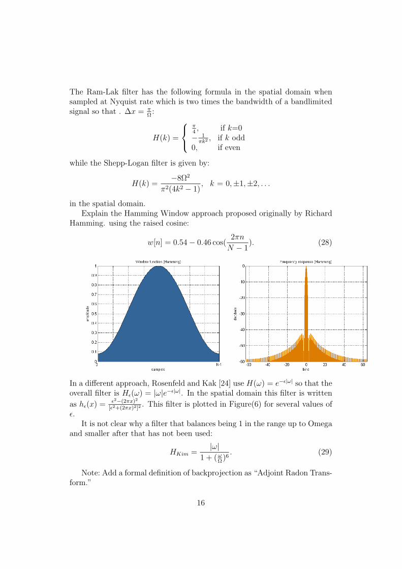
in the spatial domain.Explain the Hamming Window approach proposed originally by Richard

Hamming. using the raised cosine:

w[n] = 0.54− 0.46 cos(2πn

N − 1). (28)

In a different approach, Rosenfeld and Kak [24] use H(ω) = e−ε|ω| so that theoverall filter is Hε(ω) = |ω|e−ε|ω|. In the spatial domain this filter is written

as hε(x) = ε2−(2πx)2

[ε2+(2πx)2]2. This filter is plotted in Figure(6) for several values of

ε.It is not clear why a filter that balances being 1 in the range up to Omega

and smaller after that has not been used:

HKim =|ω|

1 + (ωΩ

)6. (29)

Note: Add a formal definition of backprojection as “Adjoint Radon Trans-form.”

16

Figure 6: The approximate reconstruction filter hε(x) from [24] plotted for ε = 5(blue), ε = 4 (red) and ε = 3 (green).

1.7 Watch out for those singularities: A review of Cal-culus

What do you do when the integrand has a singularity? Consider the integral

I =

∫ a

−a

1√xdx, (30)

where the integrand blows up at x = 0; what happens to the value of theintegral? A substitution y =

√x gives

I =1

2

∫ √a−√a

dy =√a, (31)

a finite value, even when a→ 0. Now consider the integral

II =

∫ a

−a

1

x2dx. (32)

17