Chapter 23

GEOKINETICSSections 23.1, 23.2, and 23.3 J.C. Johnston and J.C. BattisSection 23.4 J.J. Cipar and G.H. CabanissSection 23.5 J.A. Shearer and J.M. Novak Capt. USAF

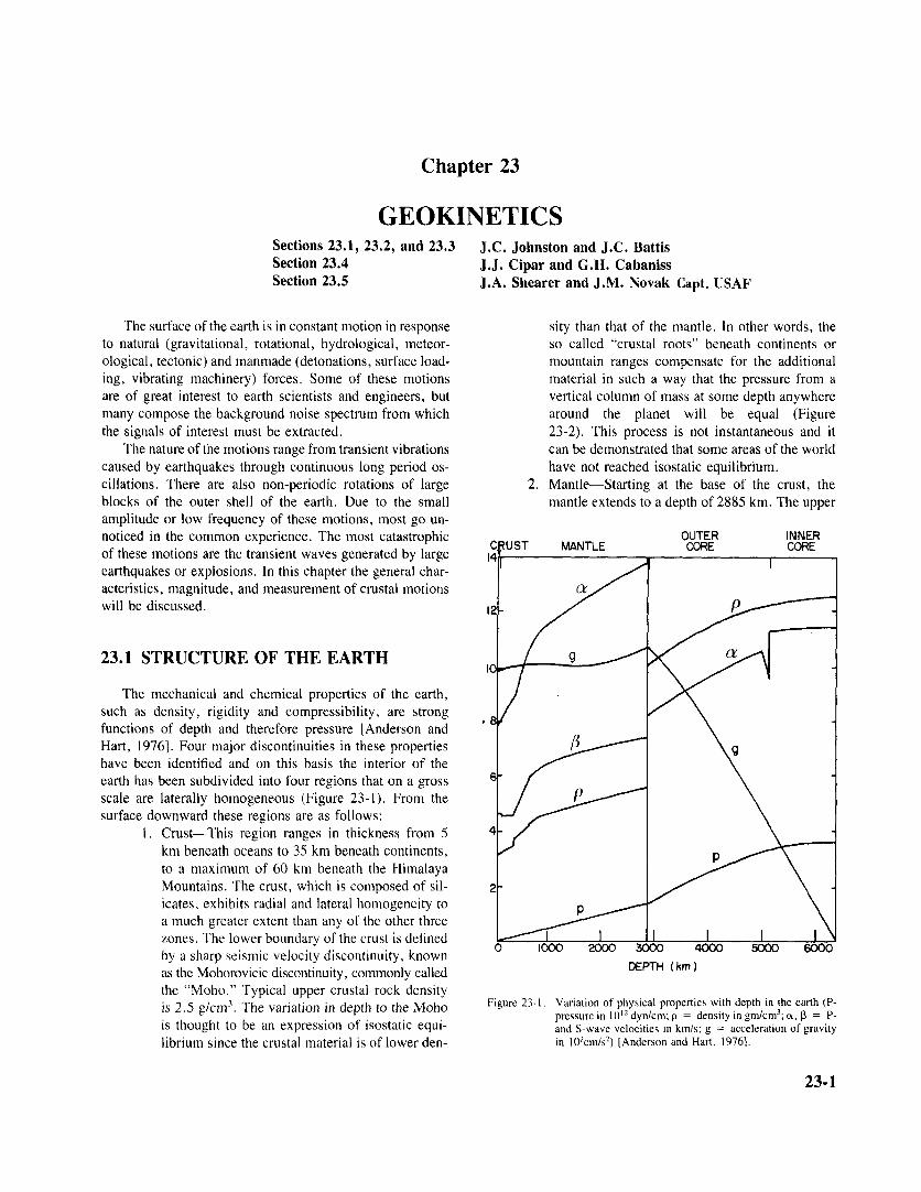
The surface of the earth is in constant motion in response sity than that of the mantle. In other words, theto natural (gravitational, rotational, hydrological, meteor- so called "crustal roots" beneath continents orological, tectonic) and manmade (detonations, surface load- mountain ranges compensate for the additionaling, vibrating machinery) forces. Some of these motions material in such a way that the pressure from aare of great interest to earth scientists and engineers, but vertical column of mass at some depth anywheremany compose the background noise spectrum from which around the planet will be equal (Figurethe signals of interest must be extracted. 23-2). This process is not instantaneous and it

The nature of the motions range from transient vibrations can be demonstrated that some areas of the worldcaused by earthquakes through continuous long period os- have not reached isostatic equilibrium.cillations. There are also non-periodic rotations of large 2. Mantle-Starting at the base of the crust, theblocks of the outer shell of the earth. Due to the small mantle extends to a depth of 2885 km. The upperamplitude or low frequency of these motions, most go un-noticed in the common experience. The most catastrophic OUTER INNERCRUST MANTLE CORE COREof these motions are the transient waves generated by largeearthquakes or explosions. In this chapter the general char-acteristics, magnitude, and measurement of crustal motions awill be discussed. 12

23.1 STRUCTURE OF THE EARTH

The mechanical and chemical properties of the earth,such as density, rigidity and compressibility, are strongfunctions of depth and therefore pressure [Anderson andHart, 1976]. Four major discontinuities in these propertieshave been identified and on this basis the interior of theearth has been subdivided into four regions that on a grossscale are laterally homogeneous (Figure 23-1). From thesurface downward these regions are as follows:

1. Crust-This region ranges in thickness from 5km beneath oceans to 35 km beneath continents,to a maximum of 60 km beneath the HimalayaMountains. The crust, which is composed of sil-icates, exhibits radial and lateral homogeneity toa much greater extent than any of the other threezones. The lower boundary of the crust is definedby a sharp seismic velocity discontinuity, knownas the Mohorovicic discontinuity, commonly called DEPTH (km)

the "Moho." Typical upper crustal rock densityis 2.5 g/cm3. The variation in depth to the Moho Figure 23-1. Variation of physical properties with depth in the earth (P-

pressure in 1012 dyn/cm; p = density in gm/cm3; a, B = P-is thought to be an expression of isostatic equi- and S-wave velocities in km/s; g = acceleration of gravity

librium since the crustal material is of lower den- in 102cm/s2) [Anderson and Hart, 1976].

23-1

CHAPTER 23

cussions can be found in geological and geophysical textspublished since 1970 (for example, Garland [1971] andWyllie [1971]). There are also several collections of sci-entific papers (such as Bird and Isacks [1972] and Cox[1973]) that illustrate the chronological development of the

CRUST theory.

Plate tectonics is primarily concerned with the kine-matics of the first several hundred kilometers below thesurface of the earth. This region is divided into two zones:the lithosphere, from the Greek word meaning "rock", and

MANTLE the asthenosphere, from the Greek word meaning "weak"CRUSTAL or lacking strength. The lithosphere exhibits finite strength

and is capable of brittle fracture, while the asthenosphere_ can be viewed as a basement of weak material having low

PRESSURE AT BOTTOM OF COLUMN P IN UNITS OF moss/length mechanical strength. The lithosphere includes the crust, but(p, h2+P2 h1)g= (P1 h3)g also extends into the upper mantle. The boundary between

these two regions is associated with the top of a seismicFigure 23-2. Isostacy principle--crustal roots under continents and moun- low velocity zone (LVZ) which typically occurs at approx-

tain ranges permit a spherical shell of equal pressure to existat some depth beneath the surface of the earth. imately 100 km depth. See Dorman [1969] and Figure

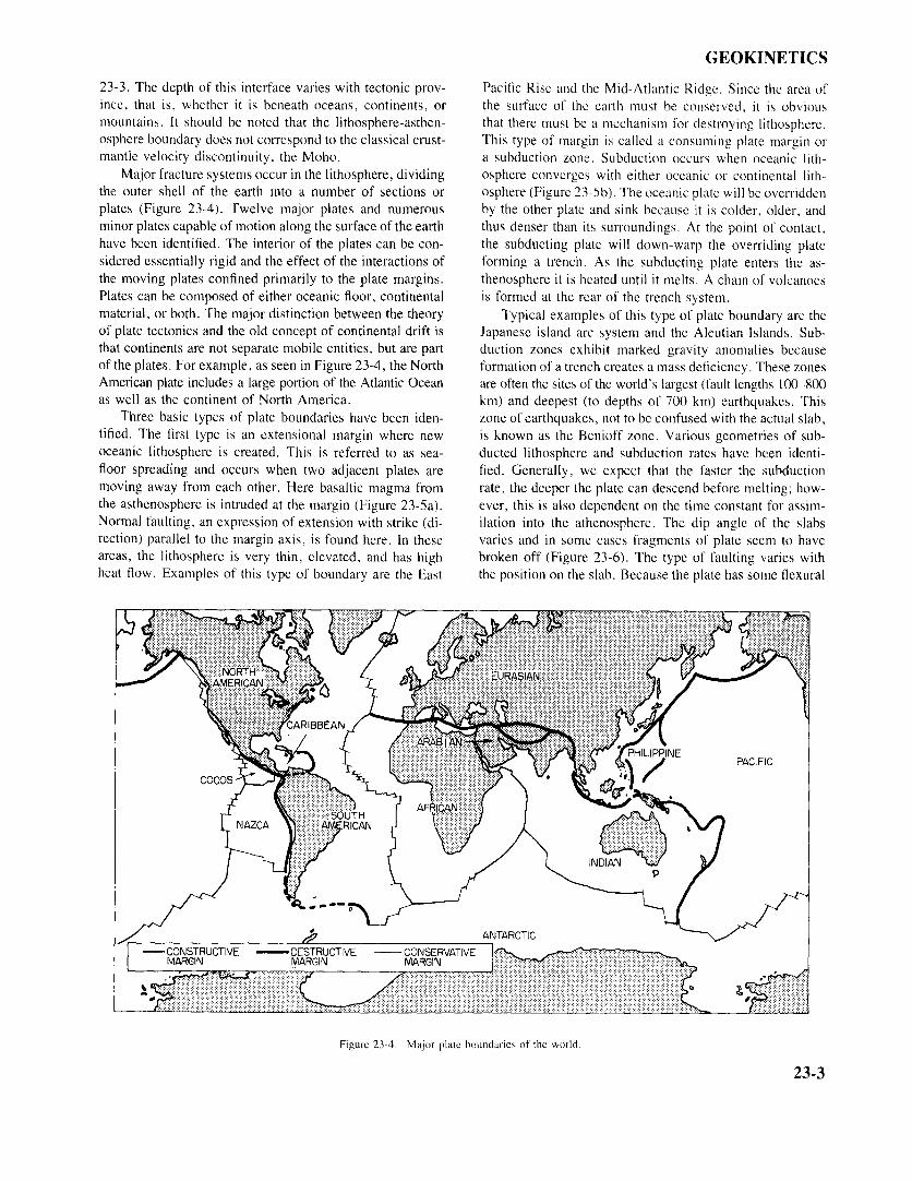
part of the mantle is probably composed mainlyof peridotites (olivines and pyroxines). The term Figure 23-3. Crust and upper mantle velocity distributions (solid line-

"pyrolite" has been applied to the composition of Pacific Ocean; dash line-Alpine; dotted line-CanadianShield). Thick horizontal bars indicate top of low velocity

the upper mantle [Clark and Ringwood, 1964]. zone [Dorman, 1969].The composition of the lower mantle is uncertain.It may consist of oxides and silicates of magne- 3.0 4.0 5.0sium and iron with small amounts of aluminumand calcium [Verhoogen et al, 1970]. Typicalmantle densities range from 3 to 5 g/cm3.

3. Outer core-This region ranges from a depth of2885 to 5155 km. It is believed to be composedof liquid iron and nickel and therefore cannotsupport shear forces. The density of the outer coreranges from approximately 9 g/cm3 to 12 g/cm3 .

4. Inner core-Beginning at a depth of 5155 km,the inner core extends to the center (6371 kmdepth) of the earth. Like the outer core, it isbelieved to consist of iron and nickel; however,as a result of the extreme pressure it is solid. Thedensity of the inner core material is approximately11 g/cm3 .

In geophysical literature there is another radial divisionof the earth into the lithosphere and the asthenosphere. Thisis primarily a division based on strength, and the boundarydoes not correspond to any of the ones previously discussed.The next section, which is an overview of the theory ofplate tectonics, is concerned with this division.

23.2 PLATE TECTONICS

The development of the theory of plate tectonics rep-resents a revolution in the understanding of the evolutionof the surface of the earth. Because the theory is referredto in several of the following sections, a brief survey of thesubject will be presented here. More comprehensive dis- SHEAR VELOCITY (km/sec)

23-2

GEOKINETICS

23-3. The depth of this interface varies with tectonic prov- Pacific Rise and the Mid-Atlantic Ridge. Since the area ofince, that is, whether it is beneath oceans, continents, or the surface of the earth must be conserved, it is obviousmountains. It should be noted that the lithosphere-asthen- that there must be a mechanism for destroying lithosphere.osphere boundary does not correspond to the classical crust- This type of margin is called a consuming plate margin ormantle velocity discontinuity, the Moho. a subduction zone. Subduction occurs when oceanic lith-

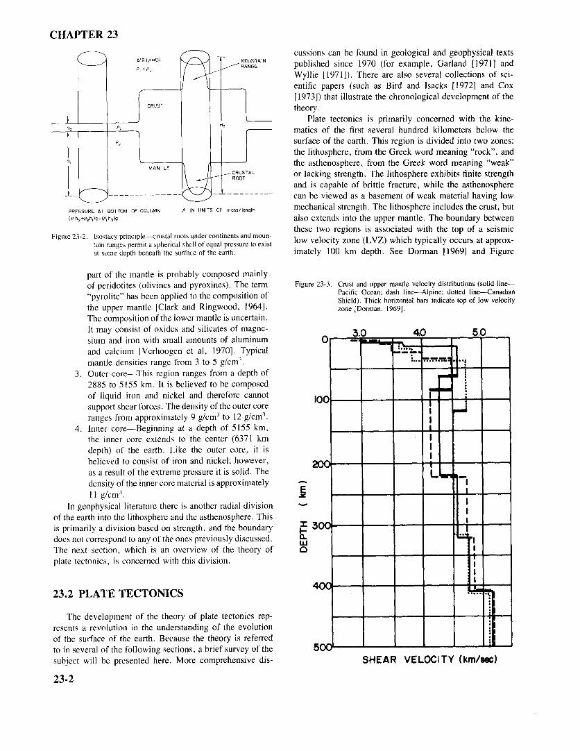
Major fracture systems occur in the lithosphere, dividing osphere converges with either oceanic or continental lith-the outer shell of the earth into a number of sections or osphere (Figure 23-5b). The oceanic plate will be overriddenplates (Figure 23-4). Twelve major plates and numerous by the other plate and sink because it is colder, older, andminor plates capable of motion along the surface of the earth thus denser than its surroundings. At the point of contact,have been identified. The interior of the plates can be con- the subducting plate will down-warp the overriding platesidered essentially rigid and the effect of the interactions of forming a trench. As the subducting plate enters the as-the moving plates confined primarily to the plate margins. thenosphere it is heated until it melts. A chain of volcanoesPlates can be composed of either oceanic floor, continental is formed at the rear of the trench system.material, or both. The major distinction between the theory Typical examples of this type of plate boundary are theof plate tectonics and the old concept of continental drift is Japanese island arc system and the Aleutian Islands. Sub-that continents are not separate mobile entities, but are part duction zones exhibit marked gravity anomalies becauseof the plates. For example, as seen in Figure 23-4, the North formation of a trench creates a mass deficiency. These zonesAmerican plate includes a large portion of the Atlantic Ocean are often the sites of the world's largest (fault lengths 100-800as well as the continent of North America. km) and deepest (to depths of 700 km) earthquakes. This

Three basic types of plate boundaries have been iden- zone of earthquakes, not to be confused with the actual slab,tified. The first type is an extensional margin where new is known as the Benioff zone. Various geometries of sub-oceanic lithosphere is created. This is referred to as sea- ducted lithosphere and subduction rates have been identi-floor spreading and occurs when two adjacent plates are fied. Generally, we expect that the faster the subductionmoving away from each other. Here basaltic magma from rate, the deeper the plate can descend before melting; how-the asthenosphere is intruded at the margin (Figure 23-5a). ever, this is also dependent on the time constant for assim-Normal faulting, an expression of extension with strike (di- ilation into the athenosphere. The dip angle of the slabsrection) parallel to the margin axis. is found here. In these varies and in some cases fragments of plate seem to haveareas, the lithosphere is very thin, elevated, and has high broken off (Figure 23-6). The type of faulting varies withheat flow. Examples of this type of boundary are the East the position on the slab. Because the plate has some flexural

AMERICAN

NAZCA AMERICAN

ANTARCTIC- CONSTRUCTIVE DESTRUCTIVE CONSERVATIVE

MARGIN MARGIN MARGIN

Figure 23-4. Major plate boundaries of the world.

23-3

CHAPTER 23

RIFT (a)ZONE (a) LITHOSPHERF

PLATE

MOTION ASTHENOSPHERE

ASTHENOSPHERE

(a) EXTENSIONAL BOUNDARY

TRENCHVOLCANO

(b)

(b) SUBDUCTION ZONES

PLATE

(c) TRANSFORM PLATE (C)

TRENCH MOUNTAINS

LITHOSPHERE

(d) ACCRETING MARGIN (d)

Figure 23-5. Plate boundary types.

rigidity, the downgoing slab actually warps upward aboutthe radius of curvature. Tensional faulting is observed inthis region. Compressional thrust faulting is found furtherdown the subducted slab. In some areas of the world, parts Figure 23-6. Various geometries of subducting slabs.

(a) shallow angleof the downgoing slab appear to be breaking off and are in (b) steep angle

tension (axis of least compressive stress is parallel to the (c) short slab

slab and dipping down). This could be caused by gravita- (d) broken slab

tional sinking [Isacks et al., 1968]. In some cases of sub-duction of oceanic lithosphere beneath continental litho- in the plate boundaries and friction between the two plates.sphere, slivers of ocean crust have been scraped off onto In this case, the Pacific plate is rotating in a counterclock-the continent. These fragments are called "ophiolites" [Gass, wise direction relative to the North American Plate.19821. It should be noted that the recycling scheme mentioned

While the combination of the spreading mid-ocean ridge above refers only to oceanic lithosphere. Continental lith-systems with the subduction zones creates a recycling scheme osphere, which is buoyant and thick, generally does notfor the surface of the earth, a third type of boundary neither subduct. As a consequence, the oldest oceanic lithospherecreates nor destroys lithosphere. If two plates do not con- (about 200 million years) is younger than most continentalverge but slide past each other, the plate margin is called lithosphere. When the collision involves continental lith-a transform or strike-slip fault. See Figure 23-5c and Wilson osphere of both plates, the buoyant forces of the overridden[1965]. The San Andreas Fault in California is the best plate produce uplift of the overriding plate resulting inknown example of a transform fault. In this case, the only mountain building forces (Figure 23-5d). The Tibetan Pla-resistance to the relative motion results from irregularities teau, site of the convergence of the India and Eurasian

23-4

GEOKINETICS

plates, is an example of this type of plate margin. The plate seems to have terminated prior to significant separation. Theapproximation becomes less useful for continent to continent Mississippi and St. Lawrence River Valleys may be regionscollisions and the plastic properties of the lithosphere must of failed rifting. This theory postulates that a plate beginsbe considered. Since continental lithosphere cannot be de- to break up because of upwelling mantle plumes which arestroyed, the oldest rocks in the world are found on the stable, convective cells of molten material that reach the surface.inactive continental shields such as Canada and Africa. Is- It can be shown that the least energy configuration for frac-land arcs, which are not part of the continental lithosphere, ture from a point source is a triple junction with radiallyare usually "scraped off' ih slivers by the overriding plate symmetric fracture arms at 120 degrees. If several of thesewhen the plate subducts. This is thought to be a mechanism spreading arms from other plumes intersect, the coalescingfor creation of the continents. arms become a spreading ridge. The third faulted arm be-

comes relatively dormant. A name sometimes applied tothese "failed arms" is alachogen.

23.2.1 Driving Mechanism

The driving mechanism for plate motion is unknown; 23.2.2 Plate Motionshowever, several hypotheses have been proposed. Initially,thermal convection cells in the mantle resulting from dis- Relative plate motions can be estimated by the analysissipation of heat in the deep mantle from radioactive decay of spreading rates at extensional margins, displacement acrosswere believed to drive the system by exerting viscous drag transform faults, and earthquake slip at subduction zones.on the bottom of the lithospheric plates. Although this mech- Spreading rates at sea floor spreading ridges are generallyanism has not been discounted, other explanations have been measured by paleomagnetic anomalies. When magma isoffered. Other hypothetical mechanisms include gravita- intruded at these ridges, it is heated past the Curie temper-tional pulling by subducting plates, pushing by injection of ature, the temperature at which material gives up its re-new crust at mid-ocean ridges (considered unlikely on the manent magnetization and realigns itself with the ambientbasis of simple energy arguments), and excitation by the magnetic field. When the magma cools it "freezes" in theChandler wobble or change in the length of day (rotation ambient magnetic field. This makes estimates of spreadingrate). In the latter, it is unclear which is the cause and which rates possible because of two facts. First, the polarity of theis the effect. earth's magnetic field reverses itself on a seemingly random

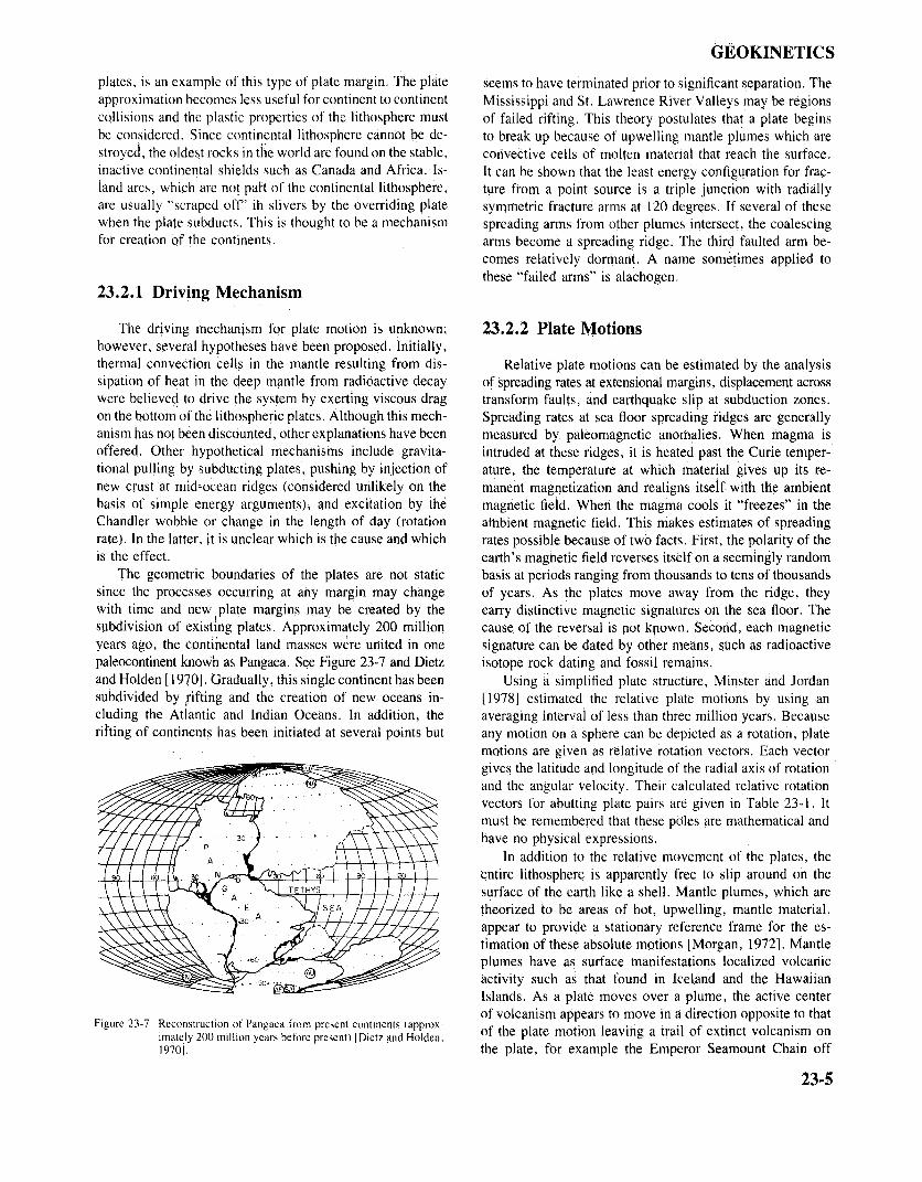
The geometric boundaries of the plates are not static basis at periods ranging from thousands to tens of thousandssince the processes occurring at any margin may change of years. As the plates move away from the ridge, theywith time and new plate margins may be created by the carry distinctive magnetic signatures on the sea floor. Thesubdivision of existing plates. Approximately 200 million cause of the reversal is not kpown. Second, each magneticyears ago, the continental land masses were united in one signature can be dated by other means, such as radioactivepaleocontinent known as Pangaea. See Figure 23-7 and Dietz isotope rock dating and fossil remains.and Holden [1970]. Gradually, this single continent has been Using a simplified plate structure, Minster and Jordansubdivided by rifting and the creation of new oceans in- [1978] estimated the relative plate motions by using ancluding the Atlantic and Indian Oceans. In addition, the averaging interval of less than three million years. Becauserifting of continents has been initiated at several points but any motion on a sphere can be depicted as a rotation, plate

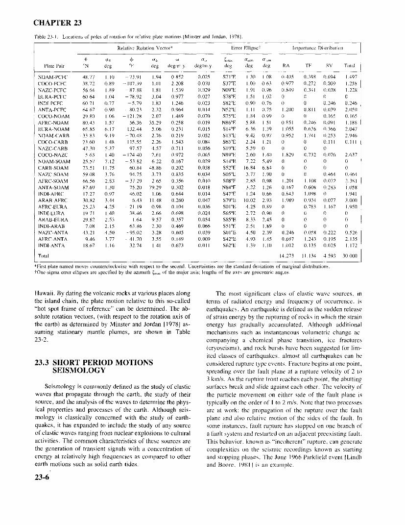
motions are given as relative rotation vectors. Each vectorgives the latitude and longitude of the radial axis of rotationand the angular velocity. Their calculated relative rotationvectors for abutting plate pairs are given in Table 23-1. Itmust be remembered that these poles are mathematical andhave no physical expressions.

In addition to the relative movement of the plates, theentire lithosphere is apparently free to slip around on thesurface of the earth like a shell. Mantle plumes, which aretheorized to be areas of hot, upwelling, mantle material,appear to provide a stationary reference frame for the es-timation of these absolute motions [Morgan, 1972]. Mantleplumes have as surface manifestations localized volcanicactivity such as that found in Iceland and the HawaiianIslands. As a plate moves over a plume, the active centerof volcanism appears to move in a direction opposite to that

Figure 23-7 Reconstruction of Pangaea from present continents (approx-imately 200 million years before present) [Dietz and Holden, of the plate motion leaving a trail of extinct volcanism on1970]. the plate, for example the Emperor Seamount Chain off

23-5

CHAPTER 23

Table 23-1. Locations of poles of rotation for relative plate motions [Minster and Jordan, 1978].

Relative Rotation Vector* Error Ellipse- Importance Distribution

0 0o O O w aw max amax omin

Plate Pair °N deg °E deg deg/m.y. deg/m.y. deg deg deg RA TF SV Total

NOAM-PCFC 48.77 1.10 73.91 1.94 0.852 0.025 S71°E 1.30 1.08 0.405 0.398 0.694 1.497COCO-PCFC 38.72 0.89 -107.39 1.01 2.208 0.070 S37°E 1.00 0.63 0.977 0.272 0.009 1.258NAZC-PCFC 56.64 1.89 -87.88 1.81 1.539 0.029 N09°E 1.91 0.96 0.849 0.341 0.038 1.228EURA-PCFC 60.64 1.04 -78.92 3.04 0.977 0.027 S78°E 1.51 1.02 0 0 0 0INDI-PCFC 60.71 0.77 -5.79 1.83 1.246 0.023 S82°E 0.90 0.76 0 0 0.246 0.246ANTA-PCFC 64.67 0.90 -80.23 2.32 0.964 0.014 N52°E 1.11 0.75 1.200 0.811 0.039 2.050COCO-NOAM 29.80 1.06 121.28 2.07 1.489 0.070 S75°E 1.84 0.99 0 0 0.165 0.165AFRC-NOAM 80.43 1.57 56.36 35.29 0.258 0.019 N86°E 5.88 1.51 0.851 0.246 0.091 1.188EURA-NOAM 65.85 6.17 132.44 5.06 0.231 0.015 S14°E 6.36 1.39 1.055 0.626 0.366 2.047NOAM-CARB -33.83 9.19 -70.48 2.76 0.219 0.052 S13°E 9.42 0.97 0.952 1.741 0.253 2.946COCO-CARB 23.60 1.48 115.55 2.26 1.543 0.084 S63°E 2.24 1.21 0 0 0.111 0.111NAZC-CARB 47.30 5.37 -97.57 4.57 0.711 0.056 S19°E 5.59 0 0 0 0COCO-NAZC 5.63 1.40 -124.40 2.61 0.972 0.065 N89°E 2.60 1.40 1.829 0.732 0.076 2.637NOAM-SOAM 25.57 7.12 -53.82 6.22 0.167 0.029 S14°E 7.22 5.49 0 0 0 0CARB-SOAM 73.51 11.75 60.84 48.86 0.202 0.038 S52°E 16.84 6.84 0 0 0 0NAZC-SOAM 59.08 3.76 - 94.75 3.73 0.835 0.034 S05°E 3.77 1.90 0 0 0.464 0.464AFRC-SOAM 66.56 2.83 -37.29 2.65 0.356 0.010 S08°E 2.85 0.98 1.201 1.108 0.072 2.381ANTA-SOAM 87.69 1.30 75.20 79.29 0.302 0.018 N84°E 3.22 1.26 0.167 0.608 0.283 1.058INDI-AFRC 17.27 0.97 46.02 1.06 0.644 0.014 S47°E 1.24 0.66 0.843 1.098 0 1.941ARAB-AFRC 30.82 3.44 6.43 11.48 0.260 0.047 S79°E 10.02 2.93 1.989 0.934 0.077 3.000AFRC-EURA 25.23 4.25 -21.19 0.98 0.104 0.036 S01°E 4.25 0.89 0 0.783 1.167 1.950INDI-EURA 19.71 1.40 38.46 2.66 0.698 0.024 S65°E 2.72 0.90 0 0 0 0ARAB-EURA 29.82 2.53 1.64 9.57 0.357 0.054 S85°E 8.33 2.45 0 0 0 0INDI-ARAB 7.08 2.15 63.86 2.30 0.469 0.066 S51°E 2.51 1.89 0 0 0 0NAZC-ANTA 43.21 4.50 -95.02 3.28 0.605 0.039 S01°E 4.50 2.39 0.246 0.058 0.222 0.526AFRC-ANTA 9.46 3.77 -41.70 3.55 0.149 0.009 S42°E 4.93 1.45 0.697 1.243 0.195 2.135INDI-ANTA 18.67 1.16 32.74 1.41 0.673 0.011 S62°E 1.39 1.10 1.012 0.135 0.025 1.172

Total 14.273 11.134 4.593 30.000

*First plate named moves counterclockwise with respect to the second. Uncertainties are the standard deviations of marginal distributions.tOne-sigma error ellipses are specified by the azimuth Xmax of the major axis; lengths of the axes are geocentric angles.

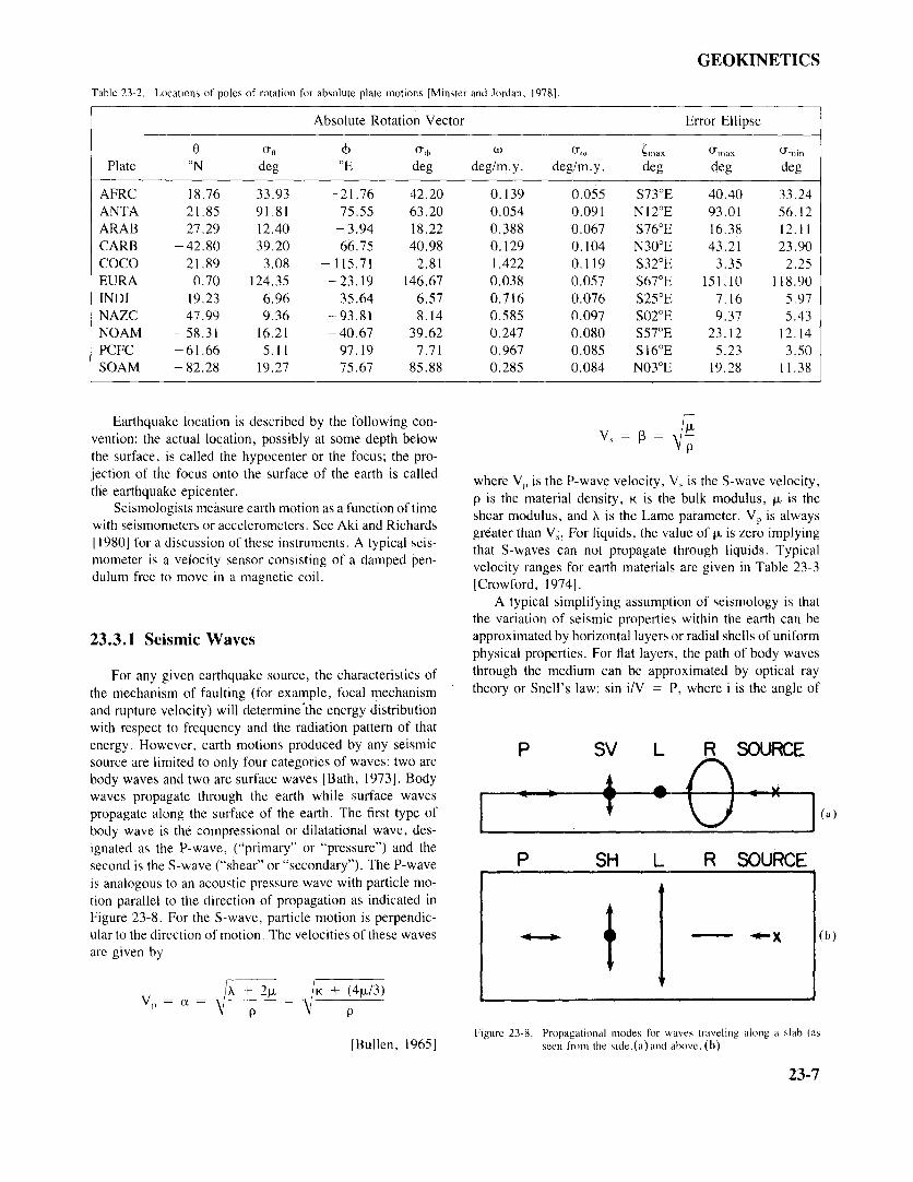
Hawaii. By dating the volcanic rocks at various places along The most significant class of elastic wave sources, inthe island chain, the plate motion relative to this so-called terms of radiated energy and frequency of occurrence, is"hot spot frame of reference" can be determined. The ab- earthquakes. An earthquake is defined as the sudden releasesolute rotation vectors, (with respect to the rotation axis of of strain energy by the rupturing of rocks in which the strainthe earth) as determined by Minster and Jordan [1978] as- energy has gradually accumulated. Although additionalsuming stationary mantle plumes, are shown in Table mechanisms such as instantaneous volumetric change ac-23-2. companying a chemical phase transition, ice fractures

(cryoseisms), and rock bursts have been suggested for lim-ited classes of earthquakes, almost all earthquakes can be

23.3 SHORT PERIOD MOTIONS considered rupture type events. Fracture begins at one point,SEISMOLOGY spreading over the fault plane at a rupture velocity of 2 to

3 km/s. As the rupture front reaches each point, the abuttingSeismology is commonly defined as the study of elastic surfaces break and slide against each other. The velocity of

waves that propagate through the earth, the study of their the particle movement on either side of the fault plane issource, and the analysis of the waves to determine the phys- typically on the order of I to 2 m/s. Note that two processesical properties and processes of the earth. Although seis- are at work: the propagation of the rupture over the faultmology is classically concerned with the study of earth- plane and also relative motion of the sides of the fault. Inquakes, it has expanded to include the study of any source some instances, fault rupture has stopped on one branch ofof elastic waves ranging from nuclear explosions to cultural a fault system and restarted on an adjacent preexisting fault.activities. The common characteristics of these sources are This behavior, known as "incoherent" rupture, can generatethe generation of transient signals with a concentration of complexities on the seismic recordings known as startingenergy at relatively high frequencies as compared to other and stopping phases. The June 1966 Parkfield event [Lindhearth motions such as solid earth tides. and Boore, 1981] is an example.

23-6

GEOKINETICS

Table 23-2. Locations of poles of rotation for absolute plate motions [Minster and Jordan, 1978].

Absolute Rotation Vector Error Ellipse

0 ao O w aw Xmax Zmin

Plate °N deg °E deg deg/m.y. deg/m.y. deg deg deg

AFRC 18.76 33.93 -21.76 42.20 0.139 0.055 S730E 40.40 33.24ANTA 21.85 91.81 75.55 63.20 0.054 0.091 N12oE 93.01 56.12ARAB 27.29 12.40 - 3.94 18.22 0.388 0.067 S76°E 16.38 12.11CARB -42.80 39.20 66.75 40.98 0.129 0.104 N30oE 43.21 23.90COCO 21.89 3.08 -115.71 2.81 1.422 0.119 S32oE 3.35 2.25EURA 0.70 124.35 -23.19 146.67 0.038 0.057 S67°E 151.10 118.90INDI 19.23 6.96 35.64 6.57 0.716 0.076 S25oE 7.16 5.97NAZC 47.99 9.36 -93.81 8.14 0.585 0.097 S02°E 9.37 5.43NOAM - 58.31 16.21 - 40.67 39.62 0.247 0.080 S57oE 23.12 12.14PCFC -61.66 5.11 97.19 7.71 0.967 0.085 S16oE 5.23 3.50SOAM -82.28 19.27 75.67 85.88 0.285 0.084 N03oE 19.28 11.38

Earthquake location is described by the following con-vention: the actual location, possibly at some depth below Vs = B =the surface, is called the hypocenter or the focus; the pro-jection of the focus onto the surface of the earth is called

where Vp is the P-wave velocity, Vs is the S-wave velocity,the earthquake epicenter. p is the material density, K is the bulk modulus, u is the

Seismologists measure earth motion as a function of time shear modulus, and X is the Lame parameter. Vp is alwayswith seismometers or accelerometers. See Aki and Richards greater than Vs. For liquids, the value of u is zero implying[1980] for a discussion of these instruments. A typical seis-

that S-waves can not propagate through liquids. Typicalmometer is a velocity sensor consisting of a damped pen-mometer is a velocity sensor consisting of a damped pen- velocity ranges for earth materials are given in Table 23-3dulum free to move in a magnetic coil. [Crowford, 1974].

A typical simplifying assumption of seismology is thatthe variation of seismic properties within the earth can be

23.3.1 Seismic Waves approximated by horizontal layers or radial shells of uniformphysical properties. For flat layers, the path of body waves

For any given earthquake source, the characteristics of through the medium can be approximated by optical raythe mechanism of faulting (for example, focal mechanism theory or Snell's law: sin i/V = P, where i is the angle ofand rupture velocity) will determine the energy distributionwith respect to frequency and the radiation pattern of thatenergy. However, earth motions produced by any seismic P SV L R SOURCEsource are limited to only four categories of waves: two arebody waves and two are surface waves [Bath, 1973]. Bodywaves propagate through the earth while surface wavespropagate along the surface of the earth. The first type ofbody wave is the compressional or dilatational wave, des-ignated as the P-wave, ("primary" or "pressure") and thesecond is the S-wave ("shear" or "secondary"). The P-wave P SH L R SOURCEis analogous to an acoustic pressure wave with particle mo-tion parallel to the direction of propagation as indicated inFigure 23-8. For the S-wave, particle motion is perpendic-ular to the direction of motion. The velocities of these waves X (b)are given by

X + 2u - K + (4 u /3 )Vp = a = =

Figure 23-8. Propagational modes for waves traveling along a slab (as[Bullen, 19651 seen from the side,(a)and above, (b)

23-7

CHAPTER 23

Table 23-3. Typical seismic velocities.

Seismic Velocity Seismic VelocityMaterial ft/s m/s

Loose and dry soils 600- 3 300 180-1 000Clay and wet soils 2 500- 6 300 760-1 900Coarse and compact soils 3 000- 8 500 910-2 600Sandstone and cemented soils 3 000-14 000 910-4 300Shale and marl 6 000-17 500 1 800-5 300Limestone--chalk 7 000-21 000 2 100-6 400Metamorphic rocks 10 000-21 000 3 000-6 400Volcanic rocks 10 000-22 000 3 000-6 700Sound plutonic rocks 13 000-25 000 4 000-7 600Jointed granite 8 000-15 000 2 400-4 600Weathered rocks 2 000-10 000 600-3 100

incidence of a ray at the interface, V is the appropriatevelocity for P or S waves and p, the ray parameter, is aconstant along the ray path. At each interface, an impinging FOCUS 1 STATION I

P or S wave can generate both reflected and transmitted Pand S waves. Thus, the potential paths over which bodywave energy can travel from the source to the point ofobservation grow quickly with an increasing number of lay-ers. Over many paths, however, insufficient energy is trans-mitted to define a distinct arrival at the observation point.

There is a standard method for identifying body wavesas they pass through the earth. See Richter [19581 and Ben-Menahem and Singh 11981] for a complete discussion. S

Briefly the convention isP P-waveS S-wave STATION 3

PP P-wave reflected once by the surfaceSS S-wave reflected once from the surface a STATION 2

PPP... SSS... Multiply reflected Ps or SsSP S wave reflected by surface changed into

P wave.PSPS... Reflected wave which changed on reflec-

tion into P or S SOLID PK Wave is transmitted through outer core MANTLE

(no shear wave in liquid outer core). Ex-ample: PKP FLUID OUTER

I Wave passes through inner core COREc Wave reflects off outer corej Wave reflects off inner core COREp,s..pP,sS.. Depth phase p and s waves travel up to

the surface from deep focus earthquakes.3Example: pP,sS \

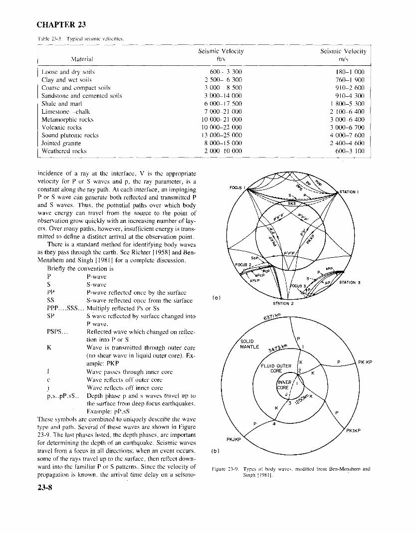
These symbols are combined to uniquely describe the wavetype and path. Several of these waves are shown in Figure PKIKP23-9. The last phases listed, the depth phases, are important

PKJKPfor determining the depth of an earthquake. Seismic wavestravel from a focus in all directions; when an event occurs, (b)some of the rays travel up to the surface, then reflect down-ward into the familiar P or S patterns. Since the velocity of Figure 23-9. Types of body waves, modified from Ben-Menahem andpropagation is known, the arrival time delay on a seismo- Singh [1981].

23-8

GEOKINETICS

gram between a pP and P for example, will be a function medium, will arrive at the receiver over different paths.of the depth. This packet will be followed by S-waves, also arriving along

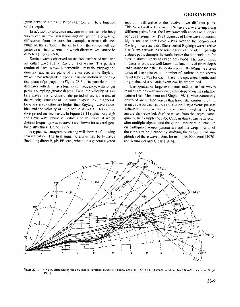
In addition to reflection and transmission, seismic body different paths. Next, the Love wave will appear with longerwaves can undergo refraction and diffraction. Because of periods arriving first. The frequency of Love waves becomesdiffraction about the core, for example, a certain distance higher and the later Love waves overlap the long-periodrange on the surface of the earth from the source will ex- Rayleigh wave arrivals. Short-period Rayleigh waves arriveperience a "shadow zone" in which direct waves cannot be last. Many arrivals in the seismogram can be identified withdetected (Figure 23-10). distinct paths through the earth; hence the nomenclature for

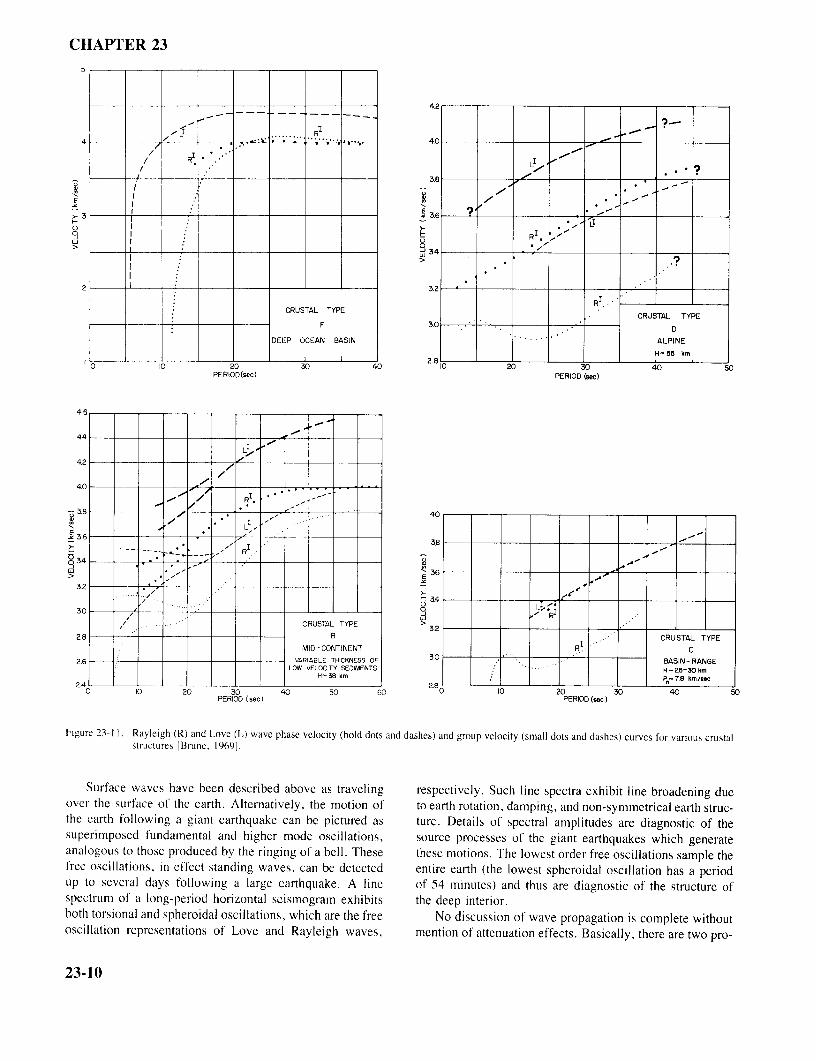
Surface waves observed on the free surface of the earth these distinct signals has been developed. The travel timesare either Love (L) or Rayleigh (R) waves. The particle of these arrivals are well known as functions of event depthmotion of Love waves is perpendicular to the propagation and distance from the observation point. By fitting the arrivaldirection and in the plane of the surface, while Rayleigh times of these phases at a number of stations to the knownwaves have retrograde elliptical particle motion in the ver- travel time curves for each phase, the epicenter, depth, andtical plane of propagation (Figure 23-8). The particle motion origin time of a seismic event can be determined.decreases with depth as a function of frequency, with longer Earthquakes or large explosions radiate surface wavesperiods sampling greater depths. Thus, the velocity of sur- in all directions with amplitudes that depend on the radiationface waves is a function of the period of the wave and of pattern [Ben-Menahem and Singh, 1981]. Most commonlythe velocity structure of the earth (dispersion). In general, observed are surface waves that travel the shortest arc of aLove wave velocities are higher than Rayleigh wave veloc- great circle between source and station. Large events possessities and the velocity of long period waves are faster than sufficient energy so that surface waves traveling the longshort period surface waves. In Figure 23-11 typical Rayleigh arc are also recorded. Surface waves from the largest earth-and Love wave phase velocities (the velocities at which quakes, for example the 1960 Chilean shock, can be detecteddistinct frequency waves travel) are shown for several geo- after multiple trips around the globe. Important informationlogic structures [Brune, 19691. on earthquake source parameters and the deep interior of

A typical seismogram recording will show the following the earth can be gleaned by studying the velocity and am-characteristics. The first signal to arrive will be P-waves plitudes of these waves. See, for example, Kanamori [1970](including direct P, pP, PP, etc.) which, in a general layered and Kanamori and Cipar [19741.

105o

Figure 23-10. P wave, diffracted by the core-mantle interface, creates a "shadow zone" at 105o to 142o distance, modified from Ben-Menahem and Singh

[1981]. 23-9

Figure 23-10 P wave diffracted by the core-mantle iterface, creates a "shadow zone" at 105° to 140o distance, modified from Ben-Menahem and Sing[1981]

23-9

CHAPTER 235

42

.

CRUSTAL TYPECRUSTAL TYPEF 30

DEEP OCEAN BASIN ALPINE

24 km 2.8 H 55 kmO 10 20 30 40 10 20 30 40 50PERIOD(sec) PERIOD (sec)

44

42

36

3.2

3.0

CRUSTAL TYPE3.2

28 CRUSTAL TYPEMID- CONTINENT RI C

2.6 VARIABLE THICKNESS OF BASIN-RANGELOW VELOCITY SEDIMENTS H- 25-30 km

H-38 km P-7.8 km/ sec0 10 20 30 40 50 60 0 10 20 30 40 50

PERIOD (sec) PERIOD (sec)

Figure 23-11. Rayleigh (R) and Love (L) wave phase velocity (bold dots and dashes) and group velocity (small dots and dashes) curves for various crustalstructures [Brune, 1969].

Surface waves have been described above as traveling respectively. Such line spectra exhibit line broadening dueover the surface of the earth. Alternatively, the motion of to earth rotation, damping, and non-symmetrical earth struc-the earth following a giant earthquake can be pictured as ture. Details of spectral amplitudes are diagnostic of thesuperimposed fundamental and higher mode oscillations, source processes of the giant earthquakes which generateanalogous to those produced by the ringing of a bell. These these motions. The lowest order free oscillations sample thefree oscillations, in effect standing waves, can be detected entire earth (the lowest spheroidal oscillation has a periodup to several days following a large earthquake. A line of 54 minutes) and thus are diagnostic of the structure ofspectrum of a long-period horizontal seismogram exhibits the deep interior.both torsional and spheroidal oscillations, which are the free No discussion of wave propagation is complete withoutoscillation representations of Love and Rayleigh waves, mention of attenuation effects. Basically, there are two pro-

23-10

GEOKINETICS

cesses at work. The first, geometric spreading, is an inverse form boundaries and at extensional margins) are generallysquare function of the distance from the source, analogous shallow with depths less than 35 km. At subduction zonesto the falloff of gravity as l/r2 where r is the distance. This the whole range of depths can be seen in a distinct pattern.occurs because the area at distance r subtended by a steradian At the trench side of the margin, the depths are shallow,(solid angle) is proportional to r2. The second type, called increasing away from the trench and under the overridingintrinsic attentuation or internal friction, is a function of the plate. The focal depth increases with the depth of penetrationdistance from the source and the wavelength of the wave, of the subducting plate into the asthenosphere.that is, the number of cycles traversed over the distance. In California, where almost all major and minor faultSome of the causes of anelastic damping are changes in zones are well mapped, most earthquakes can be associatedinternal vibrational energy in the molecules, coulomb force with pre-existing fault zones. This is readily explained by(friction) effects on the particles as a result of the physical the fact that a pre-existing fault represents a zone of weak-interaction, viscous damping, and mechanical damping dur- ness in the crust where stresses accumulate and lower stressing the acceleration of the particles. The energy is dissipated concentrations are required to cause rupturing. In other re-in the form of heat. The form of the expressions in the gions away from major plate boundaries, such as New Eng-equations for the anelastic damping factor, Q, varies and land or the Central Mississippi River Valley, the patternsthe reader should refer to one of the standard texts, for of earthquake occurrence are less clear. In these regions theexample, Aki and Richards [1980], for details. Generally, lack of surficial expression of faults due to the thickness ofa high value of Q connotes low attenuation and vice versa. soil and alluvial coverage over bedrock and the lower tem-

poral rate of occurrence of earthquakes tends to producemore diffuse patterns of seismic activity.

23.3.2 Earthquakes23.3.2.2 Measurement. The size of an earthquake can

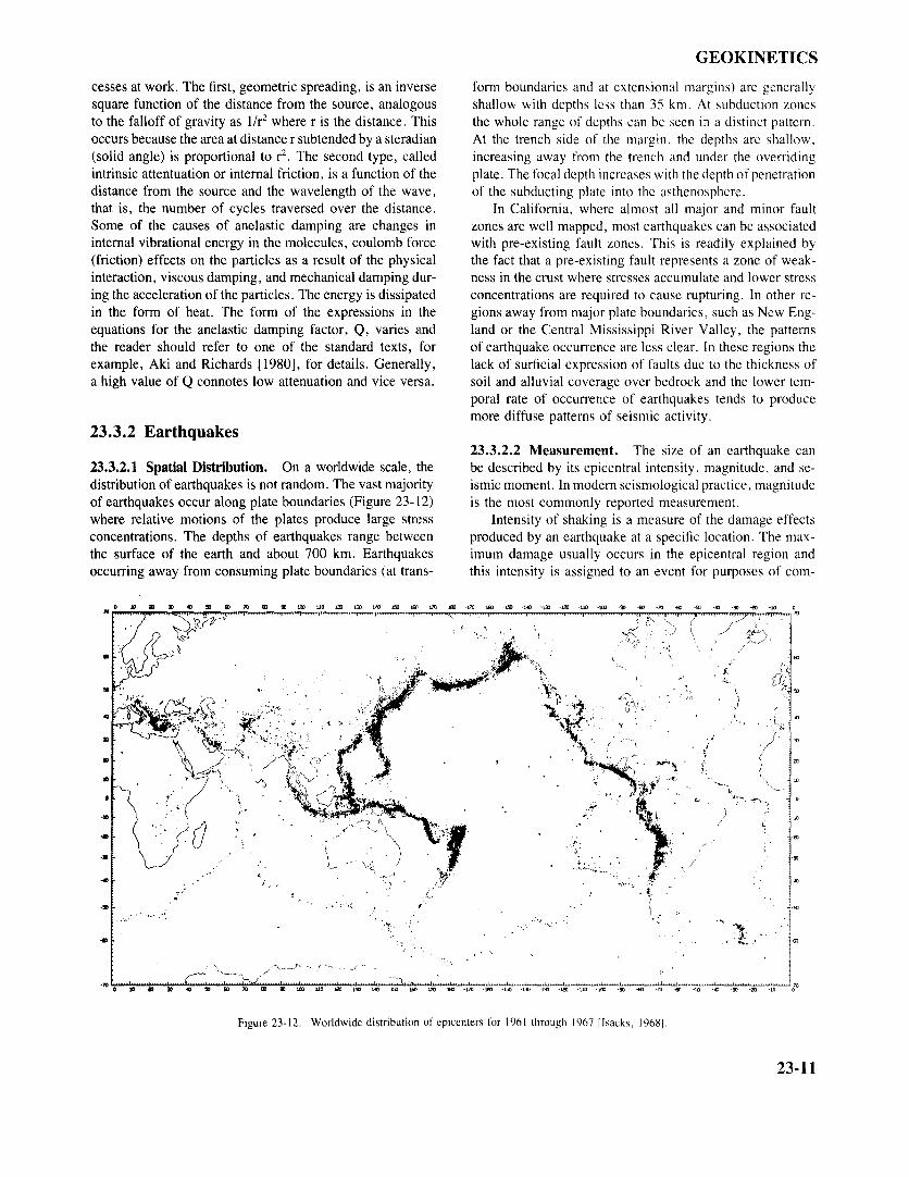
23.3.2.1 Spatial Distribution. On a worldwide scale, the be described by its epicentral intensity, magnitude, and se-distribution of earthquakes is not random. The vast majority ismic moment. In modern seismological practice, magnitudeof earthquakes occur along plate boundaries (Figure 23-12) is the most commonly reported measurement.where relative motions of the plates produce large stress Intensity of shaking is a measure of the damage effectsconcentrations. The depths of earthquakes range between produced by an earthquake at a specific location. The max-the surface of the earth and about 700 km. Earthquakes imum damage usually occurs in the epicentral region andoccurring away from consuming plate boundaries (at trans- this intensity is assigned to an event for purposes of com-

.

Figure 23-12. Worldwide distribution of epicenters for 1961 through 1967 [Isacks, 19681.

23-11

CHAPTER 23

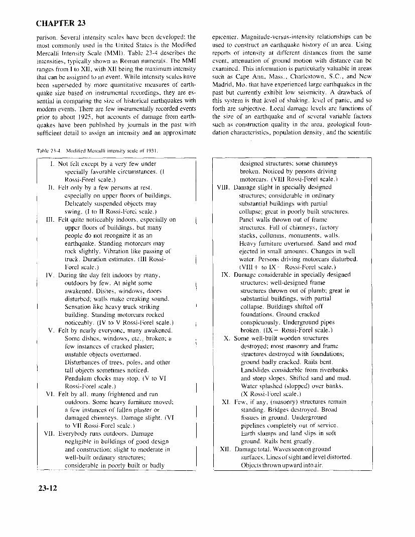
parison. Several intensity scales have been developed; the epicenter. Magnitude-versus-intensity relationships can bemost commonly used in the United States is the Modified used to construct an earthquake history of an area. UsingMercalli Intensity Scale (MMI). Table 23-4 describes the reports of intensity at different distances from the sameintensities, typically shown as Roman numerals. The MMI event, attenuation of ground motion with distance can beranges from I to XII, with XII being the maximum intensity examined. This information is particularly valuable in areasthat can be assigned to an event. While intensity scales have such as Cape Ann, Mass., Charlestown, S.C., and Newbeen superseded by more quantitative measures of earth- Madrid, Mo. that have experienced large earthquakes in thequake size based on instrumental recordings, they are es- past but currently exhibit low seismicity. A drawback ofsential in comparing the size of historical earthquakes with this system is that level of shaking, level of panic, and somodem events. There are few instrumentally recorded events forth are subjective. Local damage levels are functions ofprior to about 1925, but accounts of damage from earth- the size of an earthquake and of several variable factorsquakes have been published by journals in the past with such as construction quality in the area, geological foun-sufficient detail to assign an intensity and an approximate dation characteristics, population density, and the scientific

Table 23-4. Modified Mercalli intensity scale of 1931.

I. Not felt except by a very few under designed structures; some chimneysspecially favorable circumstances. (I broken. Noticed by persons drivingRossi-Forel scale.) motorcars. (VIII Rossi-Forel scale.)

II. Felt only by a few persons at rest, VIII. Damage slight in specially designedespecially on upper floors of buildings. structures; considerable in ordinaryDelicately suspended objects may substantial buildings with partialswing. (I to I1 Rossi-Forel scale.) collapse; great in poorly built structures.

III. Felt quite noticeably indoors, especially on Panel walls thrown out of frameupper floors of buildings, but many structures. Fall of chimneys, factorypeople do not recognize it as an stacks, collumns, monuments, walls.earthquake. Standing motorcars may Heavy furniture overturned. Sand and mudrock slightly. Vibration like passing of ejected in small amounts. Changes in welltruck. Duration estimates. (111 Rossi- water. Persons driving motorcars disturbed.Forel scale.) (VIII + to IX - Rossi-Forel scale.)

IV. During the day felt indoors by many, IX. Damage considerable in specially designedoutdoors by few. At night some structures; well-designed frameawakened. Dishes, windows, doors structures thrown out of plumb; great indisturbed; walls make creaking sound. substantial buildings, with partialSensation like heavy truck striking collapse. Buildings shifted offbuilding. Standing motorcars rocked foundations. Ground crackednoticeably. (IV to V Rossi-Forel scale.) conspicuously. Underground pipes

V. Felt by nearly everyone, many awakened. broken. (IX+ Rossi-Forel scale.)Some dishes, windows, etc., broken; a X. Some well-built wooden structuresfew instances of cracked plaster; destroyed; most masonry and frameunstable objects overturned. structures destroyed with foundations;Disturbances of trees, poles, and other ground badly cracked. Rails bent.tall objects sometimes noticed. Landslides considerble from riverbanksPendulum clocks may stop. (V to VI and steep slopes. Shifted sand and mud.Rossi-Forel scale.) Water splashed (slopped) over banks.

VI. Felt by all, many frightened and run (X Rossi-Forel scale.)outdoors. Some heavy furniture moved; XI. Few, if any, (masonry) structures remaina few instances of fallen plaster or standing. Bridges destroyed. Broaddamaged chimneys. Damage slight. (VI fissues in ground. Undergroundto VII Rossi-Forel scale.) pipelines completely out of service.

VII. Everybody runs outdoors. Damage Earth slumps and land slips in softnegligible in buildings of good design ground. Rails bent greatly.and construction; slight to moderate in XII. Damage total. Waves seen on groundwell-built ordinary structures; surfaces. Lines of sight and level distorted.considerable in poorly built or badly Objects thrown upward into air.

23-12

GEOKINETICS

integrity of the observer. If population is sparse in the ep- ration of the magnitude scale. The highest magnitude evericentral area, reports of the maximum damage may be miss- evaluated is 8.9Ms for an event near Japan on 2 Marching, thus underestimating the size of the event or mislocating 1933. This event approached the theoretical maximum mag-the epicenter. nitude based on the strengths of rocks. On the lower end

Because of these problems, data used to compile rela- of the scale, the sensitivity of the instruments and the dis-tionships of intensity to quantitative measures of earthquake tance from the event are the only limiting values with neg-size such as peak acceleration or magnitude are derived from ative magnitudes being determined for some events detectedscattered data sets. A potentially more informative intensity at very close range. Approximate relationships between theseparameter, earthquake felt area, is often computed. It is scales have been determined by several authors [for ex-defined as the area enclosed by a particular "isoseismal" ample, Nuttli, 1979; Bath, 1973]. Examples of such em-line. These lines are contours of intensity data drawn around pirical relationships are mb = 1.7 + 0.8ML - 0.01 ML2

an epicenter. Felt area is usually computed to the transition and mb = 0.56Ms + 2.9.between intensity III to IV or II to III. Local magnitude is strictly defined only for California,

The magnitude of an earthquake is calculated from an or places with very similar attenuation characteristics, whileinstrumental measurement of the amplitude of a specified the body wave and surface wave magnitudes are applied onwave packet, such as body waves or surface waves. The a worldwide basis. A common mistake found in the liter-general form is Mx = (log[A/T] or log A) + Cp + Cs + Cr, ature, especially in engineering studies, is to combine allwhere M is the magnitude, x is the subscript that identifies magnitudes or to simply assume they are all the same. Suchthe type of magnitude, A is amplitude, T is the period of a practice, as indicated by the relationships above, canthe waves (equal to approximately 1 s for body waves, 20 completely invalidate the study. Even though some reportss for surface waves), CP is the correction factor whereby and agencies may simply quote "Magnitude" or "Richterstations at all distances theoretically calculate the same mag- Magnitude", care should be taken to understand how thenitude for an event (a function of the depth of the event and magnitude was calculated. Richter magnitude often meansthe epicentral distance to the event from the station), Cs is "ML" up to M = 6.0 and "Ms" above M = 6.0. Impropera correction factor for local conditions and Cr encompasses discrimination of magnitude types causes major problemsregional correction factors allowing for effects of recording in communication and comparison of data, for examplesite, wave path, and focal mechanism [Willmore, 1979]. the estimation of maximum credible earthquakes in specificAs can be seen from the above representation, earthquake regions.magnitude is a logarithmic scale so that a change of one Relationships between magnitude and intensity have alsounit of magnitude roughly represents a change of a factor been developed and these functions have strong regionalof 10 in actual ground motion. dependencies [Brazee, 1976]. For the Western United States,

The concept of magnitude was developed by Richter in the relation between maximum intensity, Io, and body wavethe 1930's for California earthquakes and has been expanded magnitude is mb = 2.886 + 0.365Io, while for the Centralfor other areas and different wave packets by Richter and United States the relation is mb = 2.607 + 0.341 Io. Themany others. Among the most common magnitudes used importance of this regional variation and the difficulties oftoday are local magnitude (ML), the original scale proposed using intensity scales for determination of earthquake sizeby Richter (M), teleseismic body wave magnitude (mb), and are demonstrated by comparing the 1906 San Franciscosurface wave magnitude (Ms). earthquake and the 1811-1812 New Madrid earthquakes

Due to many factors, the magnitude determined for each [Nuttli, 1973]. The San Francisco earthquake probably hadscale usually will not be identical for a given earthquake, a higher magnitude than any of the New Madrid earth-The shape of the seismic wave spectrum is generally flat quakes. However, due to regional differences in seismicup to some "corner frequency" after which the amplitude wave attenuation, the San Francisco earthquake was feltdecays. The level of the flat portion is a function of the size over an area less than one-tenth of that for the largest ofof an earthquake: generally the larger the earthquake, the the New Madrid series of events. This is the result of lowerlarger the amplitude of the spectrum at a given frequency. seismic wave attenuation in the Central and Eastern UnitedThis is why mb and Ms magnitudes, which are measures of States than in California. Attenuation will be discussed fur-the amplitudes at specific frequencies, are used to measure ther in the section on seismic hazard (Section 23.3.2.5).size. However, the corner frequency moves to lower fre- The seismic moment (Mo,) of an earthquake is definedquencies and longer periods as the size of the earthquake as the product of the rigidity (u), the average offset alongincreases. Thus the relationships between magnitude scales, the fault (D) and the area of the fault (S) [Kanamori, 19771.besides being almost completely empirical, are often non- It is usually calculated in units of dyne-cm. When theselinear. Mathematically, there is no upper limit to the earth- parameters are not directly observed, spectral analysis andquake magnitude scale; however, because of this shift in speculation must be used. This measurement of earthquakecorner frequency, the size of an earthquake can get increas- size is closer to describing the physical dimensions of aingly larger with a smaller and smaller increase in M, as rupture then other kinds of measures (Io, MMI, M). Relativediscussed by Chinnery [1975]. This effect is called satu- to earthquake magnitude, which is systematically calculated

23-13

CHAPTER 23

by various international agencies such as the InternationalSeismological Centre in Edinburg, only a handful of mo-ments, mostly for larger events, have been determined. Anew type of magnitude based on the strain energy drop (themoment) has been computed for some events. It was de-veloped by Kanamori [1977] and is defined by logWo = 1.5Mw + 11.8 where W,, is the minimum strain en-ergy drop and Mw is the moment magnitude. This magnitudescale circumvents the problem of saturation of Ms that wasdiscussed earlier in this section. The great Chilean earth-quake had an Mw of 9.5 but an Ms of only 8.3.

There are numerous magnitude scales developed for usewith events too small to be recorded teleseismically (defi-nitions of this term vary; here 1000 km is considered the STRIKE=90 ° DIP=45ocutoff distance). Measurement of such events presents a (a) PURE THRUST FAULTINGproblem because the recordings are heavily influenced bythe path through the crust.

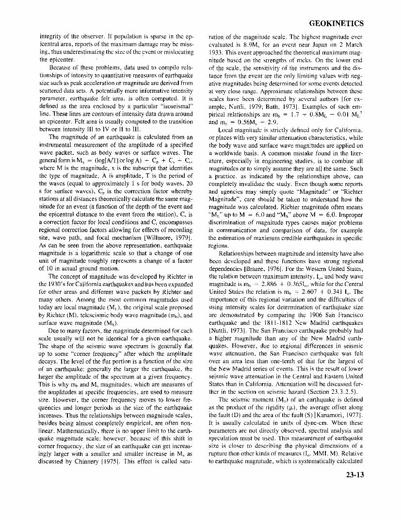
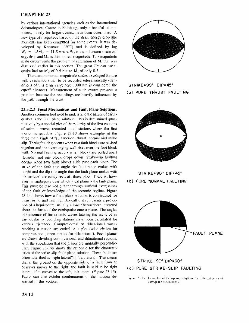
23.3.2.3 Focal Mechanisms and Fault Plane Solutions.Another common tool used to understand the nature of earth-quakes is the fault plane solution. This is determined quan-titatively by a special plot of the polarity of the first motionsof seismic waves recorded at all stations where the firstmotion is readable. Figure 23-13 shows examples of thethree main kinds of fault motion: thrust, normal and strikeslip. Thrust faulting occurs when two fault blocks are pushedtogether and the overhanging wall rises over the foot blockwall. Normal faulting occurs when blocks are pulled apart(tension) and one block drops down. Strike-slip faultingoccurs when two fault blocks slide past each other. Thestrike of the fault (the angle the fault plane makes withnorth) and the dip (the angle that the fault plane makes with STRIKE= 90 DIP=45othe surface) are easily read off these plots. There is, how-ever, an ambiguity over which focal plane is the fault plane. ( b ) PURE NORMAL FAULT INGThis must be resolved either through surficial expressionsof the fault or knowledge of the tectonic regime. Figure23-14a shows how a fault plane solution is constructed forthrust or normal faulting. Basically, it represents a projec-tion of a hemisphere, usually a lower hemisphere, centeredabout the focus of the earthquake onto a plane. The anglesof incidence of the seismic waves leaving the scene of anearthquake to recording stations have been calculated forvarious distances. Compressional or dilatational wavesreaching a station are coded on a plot (solid circles forcompressional, open circles for dilatational). Focal planes FAULT PLANEare drawn dividing compressional and dilatational regions,with the stipulation that the planes are mutually perpendic-ular. Figure 23-14b shows the rationale for the character-istics of the strike-slip fault plane solution. These faults areoften described as "right lateral" or "left lateral". This meansthat if the ground on the opposite side of a fault from an STRIKE 90o DIP=90oobserver moves to the right, the fault is said to be right (c) PURE STRIKE-SLIP FAULTINGlateral; if it moves to the left, left lateral (Figure 23-15).Faults can also exhibit combinations of the motions de- Figure 23-13. Examples of fault-plane solutions for different types ofscribed in this section. earthquake mechanisms.

23-14

GEOKINETICS

SIDE VIEW OF THRUST FAULT LEFT LATERAL MOTION

DIP ANGLESURFACE

(a)FAULT PLANE

DILATATIONAL DILATATIONAL

FIRST MOTIONS FIRST MOTIONS

PHYSICAL FAULT

OBSERVERCOMPRESSIONALFIRST MOTIONS

TOP VIEW PHYSICAL FAULT RIGHT LATERAL MOTIONPLANE

(b) FAULT PLANE

OBSERVER

TOP VIEW OF Figure 23-15. Fault motion conventionSTRIKE-SLIP FAULT (a) Observer sees land on opposite side of fault line moveto his left.

(b) Observer sees land on opposite side of fault line moveCOMPRESSIONAL DILATATIONAL to his right.

DILATATIONAL COMPRESSIONAL curves of this form are useful for areas as small as 104km2.The slope, or b-value, of the curve is normally found to lie

PHYSICAL FAULT between 0.5 and 1.5. It is not clear whether the variationsPLANE

are caused by scatter or are indicators of the seismic pro-cesses in a region. The value of "a" is highly variable,however. Obviously regions of high seismic activity, suchas southern California, have higher "a" values than less

TOP VIEW PHYSICAL FAULTPLANE seismically active regions, such as New England.

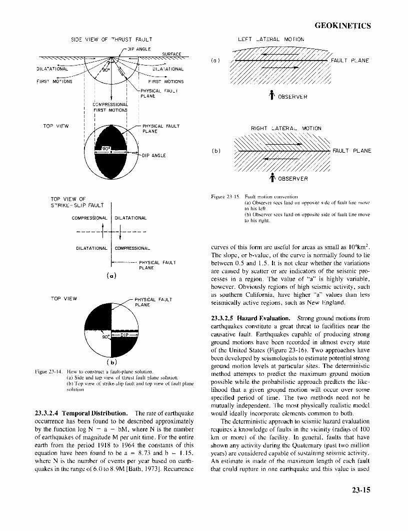
23.3.2.5 Hazard Evaluation. Strong ground motions fromearthquakes constitute a great threat to facilities near thecausative fault. Earthquakes capable of producing strongground motions have been recorded in almost every stateof the United States (Figure 23-16). Two approaches have

been developed by seismologists to estimate potential strong(b) ground motion levels at particular sites. The deterministic

Figue 23-14. How to construct a fault-plane solution.(a) Side and top view of thrust fault plane solution(b) Top view of strike-slip fault and top view of fault plane possible while the probabilistic approach predicts the like-solution lihood that a given ground motion will occur over some

specified period of time. The two methods need not bemutually independent. The most physically realistic model

23.3.2.4 Temporal Distribution. The rate of earthquake would ideally incorporate elements common to both.occurrence has been found to be described approximately The deterministic approach to seismic hazard evaluationby the function log N = a - bM, where N is the number requires a knowledge of faults in the vicinity (radius of 100of earthquakes of magnitude M per unit time. For the entire km or more) of the facility. In general, faults that haveearth from the period 1918 to 1964 the constants of this shown any activity during the Quaternary (past two millionequation have been found to be a = 8.73 and b = 1.15, years) are considered capable of sustaining seismic activity.where N is the number of events per year based on earth- An estimate is made of the maximum length of each faultquakes in the range of 6.0 to 8.9M [Bath, 1973]. Recurrence that could rupture in one earthquake and this value is used

23-15

CHAPTER 23

I

largest earthquake with a reasonable chance of occurring onMAXIMUM INTENSITIES EXPERIENCED

20o THROUGHOUT THE CENTERMINOUSUNITED STATES FROM 1928- 1973

NATIONAL OCEANIC a ATMOSPHERICADMINISTRATION

ENVIRONMENTAL DATA SERVICE

115o 1100 1050 100o 95o 90o 850 80o 750

Figure 23-16. Maximum earthquake intensities throughout the United States from 1928 to 1973 [Brazee, 1976].

to evaluate a maximum credible earthquake, that is, the ln as = 6.16 + 0.6 45ML - 1.3(R+25)largest earthquake with a reasonable chance of occurring onthe given fault. The evaluation is done using any of several ln v, = 1.63 - 0.921ML - 1.2(R +25)empirical equations relating magnitude to maximum faultrupture length [Slemmons, 1977]. One equation of this form In ds = 0.393 + 0.9 9ML - 0.88(R+25),is ML = 5.4 + 1.4 Log L, a = 0.26, where L is the lengthof the fault in kilometers [Greensfelder, 1974]. This phase where as, vs and ds are the site acceleration, velocity, andof the deterministic approach, estimating the maximum pos- displacement, ML is the event magnitude, and R is thesible earthquake, is the most difficult. Often the length of distance from the fault to the site in kilometers. Note thatthe fault is unknown and estimates of magnitude of past these equations are valid only for rock sites in the westernevents from geological examination of fault offsets do not United States. A modified acceleration function for the cen-always yield unique values. When the estimation is made, tral United States is given by Battis [1981]: ln as = 3.155strong ground motions at a site can then be evaluated using + 1.2 4 0 mb - 1.244 ln(R + 25). Further modification ofempirical relations between magnitude, distance, acceler- these equations is required to compensate for local site con-ation, velocity, or displacement. A compilation of various ditions, but these methods are beyond the scope of thisrelationships can be found in McGuire [1976]. Caution must review.be used however in selecting a set of equations since they One problem with a purely deterministic approach isare not all valid worldwide; some were developed for spe- that the return period of the maximum event may be so largecific areas, such as California. One set of equations of this that it is unreasonable logistically and financially to designtype is a relatively short lived facility to a very high value. For

23-16

GEOKINETICS

example, if a magnitude 7.0 event had a return period of BACKGROUND

100 000 years, the annual rate of occurrence would be SOURCEI x 10-5 . If the life of the structure in question is 40 years,then the probability of exceeding a magnitude 7 during the SITE

lifetime of the structure would be approximately 4 x 10-4.

At this point the probabilistic approach should be utilized.Another problem is that these relationships for accel-

eration do not predict the level of ground motion over theentire frequency range. Standardized spectra have been de-veloped (Nuclear Regulatory Guide 1.60) which can beanchored at a peak acceleration value. As yet, modificationof the shape of the spectra for the type of soil at the siteand for the magnitude of the event is not a routine process[Johnston et al., 1980].

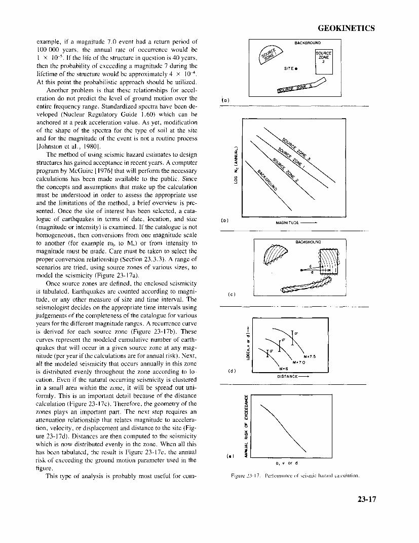
The method of using seismic hazard estimates to designstructures has gained acceptance in recent years. A computerprogram by McGuire [1976] that will perform the necessarycalculations has been made available to the public. Sincethe concepts and assumptions that make up the calculationmust be understood in order to assess the appropriate useand the limitations of the method, a brief overview is pre-sented. Once the site of interest has been selected, a cata-logue of earthquakes in terms of date, location, and size (b) MAGNITUDE

(magnitude or intensity) is examined. If the catalogue is nothomogeneous, then conversions from one magnitude scaleto another (for example mb to Ms) or from intensity to BACKGROUND

magnitude must be made. Care must be taken to select theproper conversion relationship (Section 23.3.3). A range ofscenarios are tried, using source zones of various sizes, tomodel the seismicity (Figure 23-17a). d

Once source zones are defined, the enclosed seismicityis tabulated. Earthquakes are counted according to magni- (c)tude, or any other measure of size and time interval. Theseismologist decides on the appropriate time intervals usingjudgements of the completeness of the catalogue for variousyears for the different magnitude ranges. A recurrence curveis derived for each source zone (Figure 23-17b). Thesecurves represent the modeled cumulative number of earth-quakes that will occur in a given source zone at any mag-nitude (per year if the calculations are for annual risk). Next, M=7.5

all the modeled seismicity that occurs annually in this zone M=7.0

is distributed evenly throughout the zone according to lo- (d) M=6

cation. Even if the natural occurring seismicity is clustered DISTANCE

in a small area within the zone, it will be spread out uni-formly. This is an important detail because of the distancecalculation (Figure 23-17c). Therefore, the geometry of thezones plays an important part. The next step requires anattenuation relationship that relates magnitude to accelera-tion, velocity, or displacement and distance to the site (Fig-ure 23-17d). Distances are then computed to the seismicitywhich is now distributed evenly in the zone. When all thishas been tabulated, the result is Figure 23-17e, the annualrisk of exceeding the ground motion parameter used in the a, v or d

figure.This type of analysis is probably most useful for com- Figure 23-17. Performance of seismic hazard calculation.

23-17

CHAPTER 23

parison purposes: performing this calculation for two dis-tinct sites that have a fairly accurate earthquake catalog willyield a good estimate of the relative seismic hazard of thetwo regions. Since there are some elements of the deter-ministic approach incorporated into the hazard, such aschoosing the source zone boundaries and an event uppermagnitude cutoff, this method gives more information aboutthe actual hazard to a facility during its useful lifetime (typ-ically 30 to 50 years). It also allows designers or regulatingagencies to quantitatively incorporate conservatism into thedesign or to set guidelines. Often a 10 000 year return periodis considered to be an acceptable hazard. The actual prob- SCALE: FRACTIONS OF g,THE

ability of damage to a stucture using seismic hazard and GRAVITY, ARE SHOWN.

engineering methods is called the seismic risk.Another limitation of the hazard method is that it does Figure 23-19. Contours of peak accelerations due to earthquakes at the

not include the duration of the ground motion contributing 90% confidence level for any 50-yr period [Donovan etal., 1977]. Reprinted with permission from Technology

to the annual risk. Seismic waves from a magnitude 7.0 Review, © 1977.

earthquake at 100 km distance may, for example, havehigher amplitude ground motion and longer time durationat periods greater than approximately 0.8 s than will a mag- 23.3.2.6 Premonitory Phenomena. In recent yearsnitude 5.5 which is located within 10 km of the site. Since earthquake prediction has become one of the major areasstructures respond to periodic signals more readily than to of study in seismology. The basic premise of prediction isa single spike of motion and have specific natural frequen- that as stresses accumulate in the crust, physical propertiescies, these complications should be considered. of the rock will change and these changes are detectable.

The maximum credible earthquake may have a much Compression of rock along the future earthquake rupturelonger return period than the useful life of most structures. zone is expected to produce changes in porosity, electricalProbabilistic methods are generally considered to provide resistivity, seismic velocities, water table levels, and themore realistic estimates of the ground motions and may be radon content of ground water. Tilt and elevation changesmore useful in the case of life-line structures or structures may also be indicators of future significant events. Each ofsuch as nuclear reactor facilities whose failure would pro- these phenomena are detectable by various means. For shortduce a significant threat. term prediction, abnormal animal behavior has been asso-

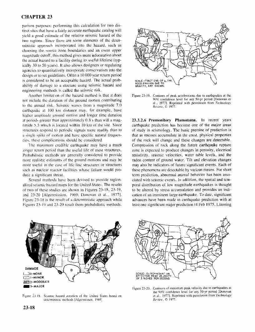
Several methods have been devised to provide region- ciated with seismic events. In addition, the spatial and tem-alized seismic hazard maps for the United States. The results poral distribution of low magnitude earthquakes is thoughtof two of these studies are shown in Figures 23-18, 23-19, to be altered by stress accumulation and provides an indi-and 23-20 [Algermission, 1969; Donovan et al., 1977]. cation of an imminent large earthquake. To date, significantFigure 23-18 is the result of a deterministic approach while advances have been made in earthquake prediction with atFigures 23-19 and 23-20 result from probabilistic methods. least one significant major prediction (4 Feb 1975, Liaoning

DAMAGE

O-NONE SCALE: 0.1 REPRESENT AN1-MINOR EFFECTIVE PEAK VELOCITY

OF 3 INCHES PER SECOND.2-MODERATE

3-MAJOR Figure 23-20. Contours of maximum peak velocity due to earthquakes atthe 90% confidence level for any 50-yr period [Donovan

Figure 23 18. Seismic hazard zonation of the United States based on et al., 1977]. Reprinted with permission from Technology

deterministic methods [Algermissen, 1969]. Review, © 1977.

23-18

GEOKINETICS

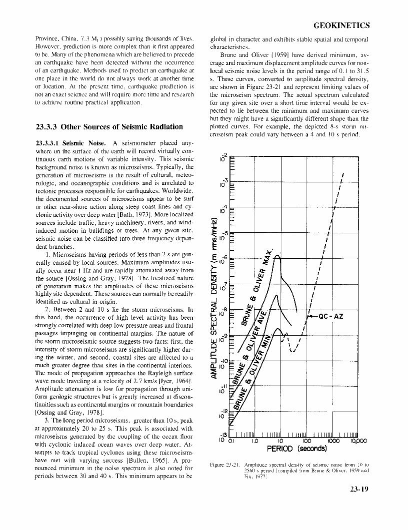
Province, China, 7.3 ML) possibly saving thousands of lives. global in character and exhibits stable spatial and temporalHowever, prediction is more complex than it first appeared characteristics.to be. Many of the phenomena which are believed to precede Brune and Oliver [1959] have derived minimum, av-an earthquake have been detected without the occurrence erage and maximum displacement amplitude curves for non-of an earthquake. Methods used to predict an earthquake at local seismic noise levels in the period range of 0.1 to 3 1.5one place in the world do not always work at another time s. These curves, converted to amplitude spectral density,or location. At the present time, earthquake prediction is are shown in Figure 23-21 and represent limiting values ofnot an exact science and will require more time and research the microseism spectrum. The actual spectrum calculatedto achieve routine practical application. for any given site over a short time interval would be ex-

pected to lie between the minimum and maximum curvesbut they might have a significantly different shape than the

23.3.3 Other Sources of Seismic Radiation plotted curves. For example, the depicted 8-s storm mi-croseism peak could vary between a 4 and 10 s period.

23.3.3.1 Seismic Noise. A seismometer placed any-where on the surface of the earth will record virtually con- -2tinuous earth motions of variable intensity. This seismic 10background noise is known as microseisms. Typically, thegeneration of microseisms is the result of cultural, meteo-rologic, and oceanographic conditions and is unrelated to 10-3tectonic processes responsible for earthquakes. Worldwide,the documented sources of microseisms appear to be surfor other near-shore action along steep coast lines and cy- -4clonic activity over deep water [Bath, 1973]. More localized l0-4sources include traffic, heavy machinery, rivers, and wind-induced motion in buildings or trees. At any given site,seismic noise can be classified into three frequency depen- 10-5dent branches.

1. Microseisms having periods of less than 2 s are gen- 6erally caused by local sources. Maximum amplitudes usu- 10-6ally occur near 1 Hz and are rapidly attenuated away fromthe source [Ossing and Gray, 1978]. The localized natureof generation makes the amplitudes of these microseisms 10-7highly site dependent. These sources can normally be readilyidentified as cultural in origin.

2. Between 2 and 10 s lie the storm microseisms. In -8this band, the occurrence of high level activity has beenstrongly correlated with deep low pressure areas and frontalpassages impinging on continental margins. The nature ofthe storm microseismic source suggests two facts: first, the 10-9intensity of storm microseisms are significantly higher dur-ing the winter, and second, coastal sites are affected to amuch greater degree than sites in the continental interiors. 10-10The mode of propagation approaches the Rayleigh surfacewave mode traveling at a velocity of 2.7 km/s [Iyer, 1964.Amplitude attenuation is low for propagation through uni- 10-11form geologic structures but is greatly increased at discon-tinuities such as continental margins or mountain boundaries[Ossing and Gray, 1978]. -12

3. The long period microseisms, greater than 10 s, peak 10-12at approximately 20 to 25 s. This peak is associated withmicroseisms generated by the coupling of the ocean floor -13

10-13with cyclonic induced ocean waves over deep water. At-tempts to track tropical cyclones using these microseisms PERIOD (seconds)have met with varying success IBullen, 1965]. A pro-have met with varying success Bullen, 1965]. A pro- Figure 23-21. Amplitude spectral density of seismic noise from 10 tonounced minimum in the noise spectrum is also noted for 2560 s period [compiled from Brune & Oliver. 1959 and

periods between 30 and 40 s. This minimum appears to be Fix. 19721.

23-19

CHAPTER 23

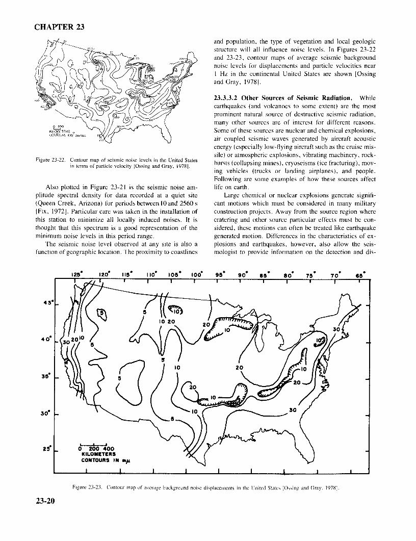
and population, the type of vegetation and local geologicstructure will all influence noise levels. In Figures 23-22and 23-23, contour maps of average seismic backgroundnoise levels for displacements and particle velocities nearI Hz in the continental United States are shown [Ossing

23.3.3.2 Other Sources of Seismic Radiation. Whileearthquakes (and volcanoes to some extent) are the mostprominent natural source of destructive seismic radiation,many other sources are of interest for different reasons.

KILOMETERS Some of these sources are nuclear and chemical explosions,CONTOURS X10-7 cm/sec air coupled seismic waves generated by aircraft acoustic

energy (especially low-flying aircraft such as the cruise mis-sile) or atmospheric explosions, vibrating machinery, rock-

Figure 23-22. Contour map of seismic noise levels in the United States bursts (collapsing mines) cryoseisms (ice fracturing), mov-in terms of particle velocity [Ossing and Gray, 1978].

ing vehicles (trucks or landing airplanes), and people.Following are some examples of how these sources affect

Also plotted in Figure 23-21 is the seismic noise am- life on earth.plitude spectral density for data recorded at a quiet site Large chemical or nuclear explosions generate signifi-(Queen Creek, Arizona) for periods between 10 and 2560 s cant motions which must be considered in many military[Fix, 19721. Particular care was taken in the installation of construction projects. Away from the source region wherethis station to minimize all locally induced noises. It is cratering and other source particular effects must be con-thought that this spectrum is a good representation of the sidered, these motions can often be treated like earthquakeminimum noise levels in this period range. generated motion. Differences in the characteristics of ex-

The seismic noise level observed at any site is also a plosions and earthquakes, however, also allow the seis-function of geographic location. The proximity to coastlines mologist to provide information on the detection and dis-

125' 120' 115' 110 105" 100' 95' 90' 85' 80' 75' 70' 65

45'

35'

KILOMETERSCONTOURS in mu

I I I

Figure 23-23. Contour map of average background noise displacements in the United States [Ossing and Gray. 1978].

23-20

GEOKINETICS

crimination of nuclear explosions for the purpose of test ban other manifestation of tectonic processes, are capable oftreaty verification. In the siting of motion sensitive instru- producing large. if localized. motion.ments, local disturbances caused by any source should be Recent tectonic theory has given the broad picture ofconsidered, especially where large concrete structures are relative motions between rigid plates, but the details areconstructed. Vibrations caused by even small quarry blasts considerably blurred for several reasons. First, the plateduring the critical curing period can prevent the proper cohe- boundaries are not simple discontinuities but are gener-sion from developing. ally zones up to 100 km or more in width where strain

The fact that moving vehicles and personnel produce can accumulate. A second problem is that plate tectonicsseismic signals has been used to develop security systems does not explain crustal motions in plate interiors. An-and methods of remote battlefield sensing. Pressure waves other problem of a different nature is the proclivity of manygenerated by military aircraft can, under certain conditions, investigators to discover "micro-plates". Then, of course,couple with the ground to produce large amplitude seismic there are large-scale secular motions that have no directmotions which could affect ground facilities or be used to relationship to plate tectonics, for example, the mid-con-track the aircraft. tinental downwarps associated with deposition in sedimen-

The study of seismic sources in the high frequency re- tary basins.gime has almost unlimited practical applications in geologicexploration, nuclear detection, and earthquake prediction. 23.4.1.1 Horizontal Motions. Almost all earthquakes that

cause observable surface displacements are associated withfaults or fault zones. Coseismic fault displacements range

23.4 LONG PERIOD AND SECULAR from negligible for small earthquakes, to several centimetersfor magnitude 5, to several meters over hundreds of kilo-

EARTH MOTIONS meters for magnitude 9 shocks. The maximum total dis-placement for the great Alaskan earthquake of 1964 was

This section briefly treats measurement of crustal motion placement for the great Alaskan earthquake of 1964 wasover 25 m. The ratio of displacement to fault length rangesand puts some bounds on the magnitude of such deforma- from 10-4 to 10-6. Well-defined, natural or artificial (plannedtions and the accuracy of the observations. Some of the or fortuitous) linear or planar features (for example, fences,most important techniques used are from the field of ge- alignment arrays, stream channels, or shorelines) crossingodesy, which is reviewed in Chapter 24. In the first sub- the fault can be used to determine the offset. Repeatedsection, details of the motions caused by tectonic processes, geodetic surveys (Chapter 24) are also made to determinewhich were reviewed in Section 23.2 will be examined; in both earthquake displacements and accumulation of strain.the second, the earth tides; and in the third, other more The U.S. Geological Survey runs an active deformationlocalized types of motions, which often form the noise back- monitoring program in California, using laser geodimetersground and hinder the performance of instruments and sys- to measure the distances among benchmarks in several geo-tems. Specifically excluded from consideration are various detic networks [Savage et al., 1981]. The formal errorsgeological processes, such as soil creep, landslides, gla- (standard deviations) in these surveys are between 10-6 andciological activity, and volcanic activity, all of which can l0-7 for lines between 20 and 50 km long. Most of the errorexhibit substantial motions. is attributable to variations of the index of refraction along

the line of sight. The strain accumulation rate in the SanAndreas fault zone is about 0.3 x 10-6/yr, or where the

23.4.1 Tectonic Motions motion is creep on the faults themselves with little or nostrain buildup, about 3-5cm/yr. Thus the expected line length

We know from geological and paleomagnetic studies changes are of the order of the present day survey accuracythat portions of the earth have moved, at least in a relative and several years must elapse between surveys before re-sense, thousands of kilometers horizontally and tens of kil- liable results can be obtained. Since several crustal platesometers vertically (the top of Mt. Everest is marine lime- converge in Japan, the deformation rate is high and thestone). We also have found from such studies that these motion pattern complex [Mogi, 1981]. Similar programsmovement velocities are not constant but are discontinuous, are in progress in Turkey, India, New Zealand, the USSR,episodic, or even cyclical. One of the main challenges in Central America, Alaska, Canada, and many others. Seesolid earth geophysics is to directly measure such motions, Simpson and Richards [1981] for examples.relate them to the past rates determined geologically orpaleomagnetically, and develop empirical or physical models 23.4.1.2 Vertical Displacements. Secular vertical crus-to predict future motions. These goals are not without prac- tal motions rarely exceed I mm/yr. Some exceptions aretical application, for the most dramatic form of tectonic Japan (7 mm/yr in some regions), where tectonic activitymotion is the sudden release of accumulated strain during is high, the Hudson Bay region (10 mm/yr), which is stillmajor earthquakes with the concurrent generation of poten- responding to the removal of the continental ice sheettially destructive seismic waves. Volcanoes, which are an- 10 000 years ago, and several other, usually local, areas.

23-21

CHAPTER 23

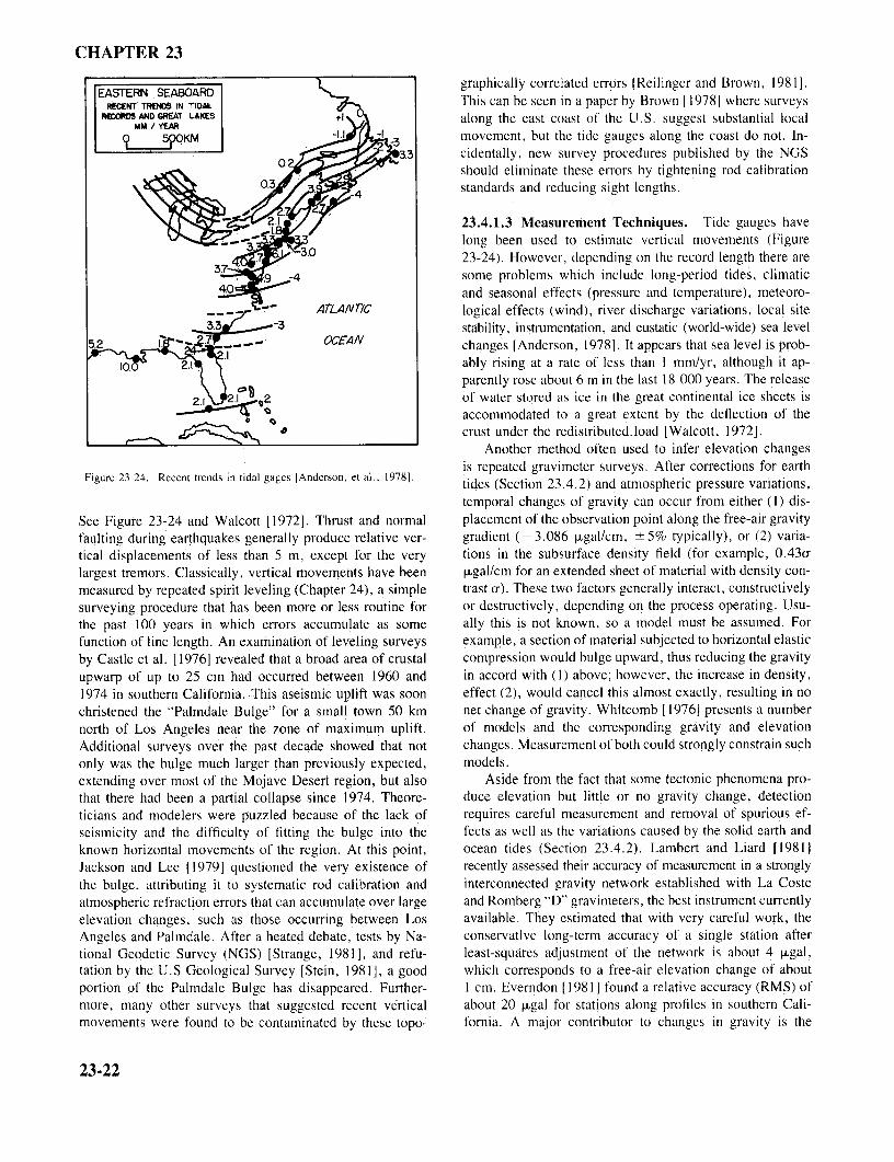
_ EASTERN SEABOARD graphically correlated errors [Reilinger and Brown, 1981].RECENT TRENDS IN TIDAL This can be seen in a paper by Brown 11978] where surveys

RECORDS AND GREAT LAKES along the east coast of the U.S. suggest substantial local

500KM movement, but the tide gauges along the coast do not. In-cidentally, new survey procedures published by the NGSshould eliminate these errors by tightening rod calibrationstandards and reducing sight lengths.

23.4.1.3 Measurement Techniques. Tide gauges havelong been used to estimate vertical movements (Figure

However, depending on the record length there aresome problems which include long-period tides, climaticand seasonal effects (pressure and temperature), meteoro-

ATLANLIC logical effects (wind), river discharge variations, local site

OCEAN stability, instrumentation, and eustatic (world-wide) sea levelchanges [Anderson, 1978]. It appears that sea level is prob-

ably rising at a rate of less than l mm/yr, although it ap-parently rose about 6 m in the last 18 000 years. The releaseof water stored as ice in the great continental ice sheets isaccommodated to a great extent by the deflection of thecrust under the redistributed.load [Walcott, 1972].

Another method often used to infer elevation changesis repeated gravimeter surveys. After corrections for earth

Figure 23-24. Recent trends in tidal gages [Anderson, et al., 1978]. tides (Section 23.4.2) and atmospheric pressure varitions,tides (Section 23.4.2) and atmospheric pressure variations,temporal changes of gravity can occur from either (1) dis-

See Figure 23-24 and Walcott [1972]. Thrust and normal placement of the observation point along the free-air gravityfaulting during earthquakes generally produce relative ver- gradient (- 3.086 ugal/cm, + 5% typically), or (2) varia-tical displacements of less than 5 m, except for the very tions in the subsurface density field (for example, 0.43alargest tremors. Classically, vertical movements have been ugal/cm for an extended sheet of material with density con-measured by repeated spirit leveling (Chapter 24), a simple trast a). These two factors generally interact, constructivelysurveying procedure that has been more or less routine for or destructively, depending on the process operating. Usu-the past 100 years in which errors accumulate as some ally this is not known, so a model must be assumed. Forfunction of line length. An examination of leveling surveys example, a section of material subjected to horizontal elasticby Castle et al. [1976] revealed that a broad area of crustal compression would bulge upward, thus reducing the gravityupwarp of up to 25 cm had occurred between 1960 and in accord with (l) above; however, the increase in density,1974 in southern California. This aseismic uplift was soon effect (2), would cancel this almost exactly, resulting in nochristened the "Palmdale Bulge" for a small town 50 km net change of gravity. Whitcomb [1976] presents a numbernorth of Los Angeles near the zone of maximum uplift. of models and the corresponding gravity and elevationAdditional surveys over the past decade showed that not changes. Measurement of both could strongly constrain suchonly was the bulge much larger than previously expected, models.extending over most of the Mojave Desert region, but also Aside from the fact that some tectonic phenomena pro-that there had been a partial collapse since 1974. Theore- duce elevation but little or no gravity change, detectionticians and modelers were puzzled because of the lack of requires careful measurement and removal of spurious ef-seismicity and the difficulty of fitting the bulge into the fects as well as the variations caused by the solid earth andknown horizontal movements of the region. At this point, ocean tides (Section 23.4.2). Lambert and Liard [19811Jackson and Lee [1979] questioned the very existence of recently assessed their accuracy of measurement in a stronglythe bulge, attributing it to systematic rod calibration and interconnected gravity network established with La Costeatmospheric refraction errors that can accumulate over large and Romberg "D" gravimeters, the best instrument currentlyelevation changes, such as those occurring between Los available. They estimated that with very careful work, theAngeles and Palmdale. After a heated debate, tests by Na- conservative long-term accuracy of a single station aftertional Geodetic Survey (NGS) [Strange, 1981], and refu- least-squares adjustment of the network is about 4 ugal,tation by the U.S Geological Survey [Stein, 1981], a good which corresponds to a free-air elevation change of aboutportion of the Palmdale Bulge has disappeared. Further- l cm. Everndon [1981] found a relative accuracy (RMS) ofmore, many other surveys that suggested recent vertical about 20 ugal for stations along profiles in southern Cali-movements were found to be contaminated by these topo- fornia. A major contributor to changes in gravity is the

23-22

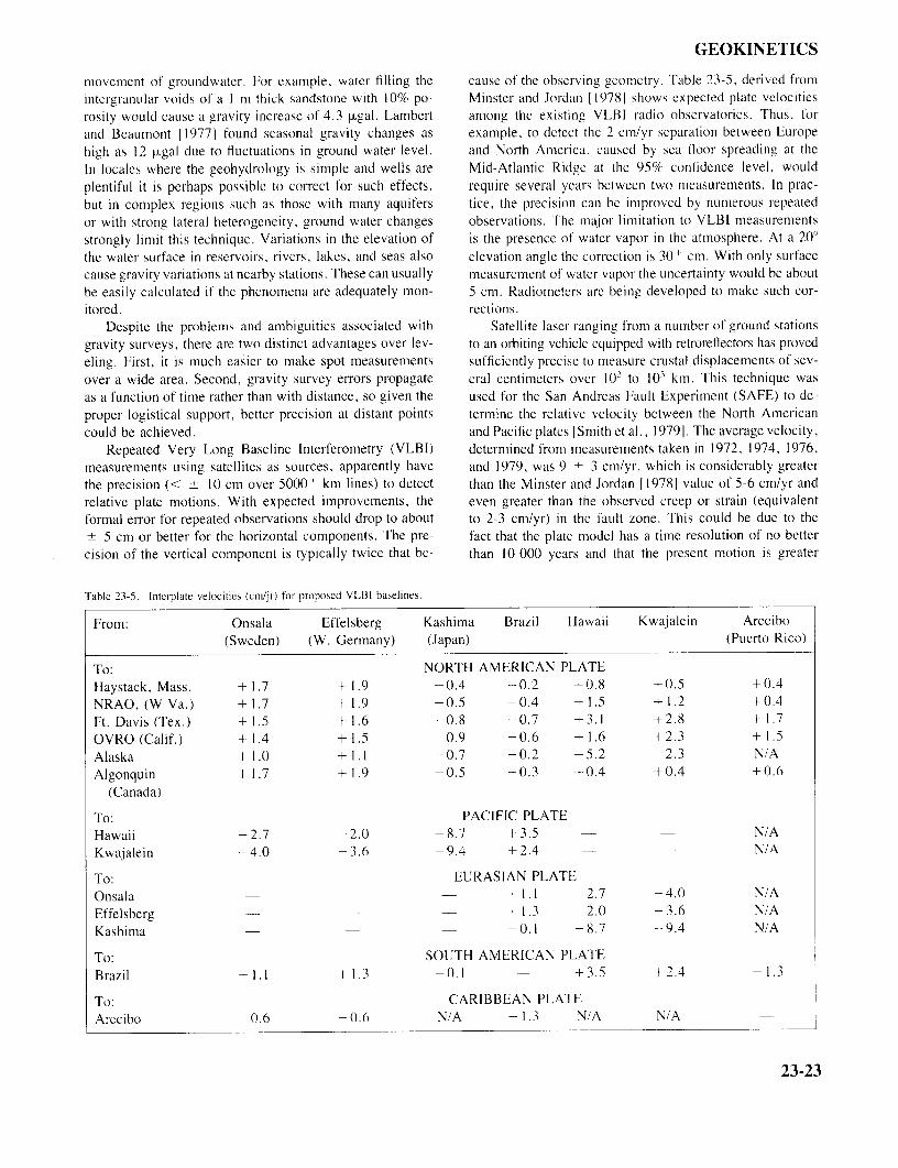
GEOKINETICS

movement of groundwater. For example, water filling the cause of the observing geometry. Table 23-5, derived fromintergranular voids of a I m thick sandstone with 10% po- Minster and Jordan 119781 shows expected plate velocitiesrosity would cause a gravity increase of 4.3 ugal. Lambert among the existing VLBI radio observatories. Thus, forand Beaumont [19771 found seasonal gravity changes as example, to detect the 2 cm/yr separation between Europehigh as 12 ugal due to fluctuations in ground water level. and North America, caused by sea floor spreading at the

In locales where the geohydrology is simple and wells are Mid-Atlantic Ridge at the 95% confidence level, wouldplentiful it is perhaps possible to correct for such effects, require several years between two measurements. In prac-but in complex regions such as those with many aquifers tice, the precision can be improved by numerous repeatedor with strong lateral heterogeneity, ground water changes observations. The major limitation to VLBI measurementsstrongly limit this technique. Variations in the elevation of is the presence of water vapor in the atmosphere. At a 20°

the water surface in reservoirs, rivers, lakes, and seas also elevation angle the correction is 30 + cm. With only surfacecause gravity variations at nearby stations. These can usually measurement of water vapor the uncertainty would be aboutbe easily calculated if the phenomena are adequately mon- 5 cm. Radiometers are being developed to make such cor-itored. rections.

Despite the problems and ambiguities associated with Satellite laser ranging from a number of ground stationsgravity surveys, there are two distinct advantages over lev- to an orbiting vehicle equipped with retroreflectors has provedeling. First, it is much easier to make spot measurements sufficiently precise to measure crustal displacements of sev-over a wide area. Second, gravity survey errors propagate eral centimeters over 102 to 103 km. This technique wasas a function of time rather than with distance, so given the used for the San Andreas Fault Experiment (SAFE) to de-proper logistical support, better precision at distant points termine the relative velocity between the North Americancould be achieved. and Pacific plates [Smith et al., 19791. The average velocity,

Repeated Very Long Baseline Interferometry (VLBI) determined from measurements taken in 1972, 1974, 1976,measurements using satellites as sources, apparently have and 1979, was 9 + 3 cm/yr, which is considerably greaterthe precision (< + 10 cm over 5000 + km lines) to detect than the Minster and Jordan 119781 value of 5-6 cm/yr andrelative plate motions. With expected improvements, the even greater than the observed creep or strain (equivalentformal error for repeated observations should drop to about to 2-3 cm/yr) in the fault zone. This could be due to the+ 5 cm or better for the horizontal components. The pre- fact that the plate model has a time resolution of no bettercision of the vertical component is typically twice that be- than 10 000 years and that the present motion is greater

Table 23-5. Interplate velocities (cm/jr) for proposed VLBI baselines.

From: Onsala Effelsberg Kashima Brazil Hawaii Kwajalein Arecibo(Sweden) (W. Germany) (Japan) (Puerto Rico)

To: NORTH AMERICAN PLATEHaystack, Mass. + 1.7 + 1.9 -0.4 -0.2 +0.8 +0.5 +0.4

NRAO, (W Va.) + 1.7 + 1.9 -0.5 -0.4 + 1.5 + 1.2 +0.4

Ft. Davis (Tex.) + 1.5 +1.6 -0.8 -0.7 +3.1 +2.8 +1.7OVRO (Calif.) + 1.4 + 1.5 -0.9 -0.6 + 1.6 +2.3 +1.5Alaska + 1.0 +1.1 -0.7 -0.2 -5.2 -2.3 N/AAlgonquin + 1.7 + 1.9 -0.5 -0.3 +0.4 +0.4 +0.6

(Canada)

To: PACIFIC PLATEHawaii - 2.7 - 2.0 8.7 + 3.5 N/AKwajalein -4.0 -3.6 -9.4 +2.4 - N/A

To: EURASIAN PLATEOnsala + 1.1 2.7 4.0 N/A

Effelsberg + 1.3 2.0 -3.6 N/AKashima -0.1 - 8.7 -9.4 N/A

To: SOUTH AMERICAN PLATEBrazil + 1.1 + 1.3 0.1 +3.5 +2.4 1.3

To: CARIBBEAN PLATEArecibo 0.6 0.6 N/A -- 1.3 N/A N/A

23-23

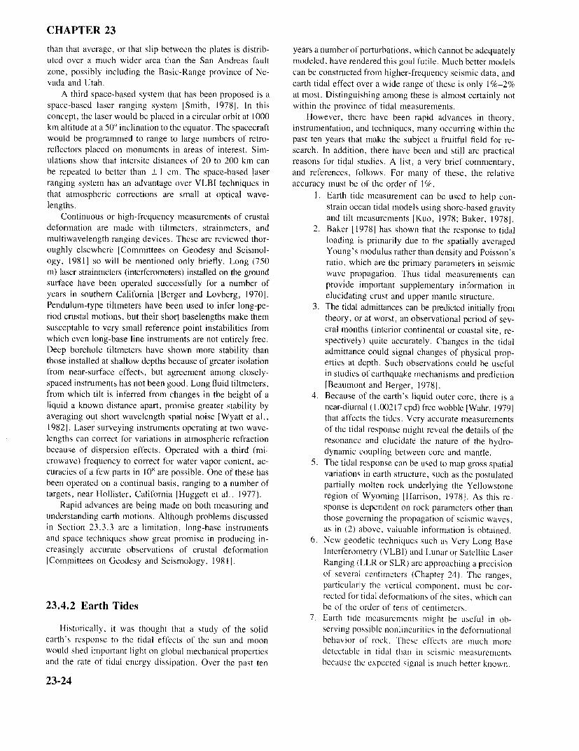
CHAPTER 23

than that average, or that slip between the plates is distrib- years a number of perturbations, which cannot be adequatelyuted over a much wider area than the San Andreas fault modeled, have rendered this goal futile. Much better modelszone, possibly including the Basic-Range province of Ne- can be constructed from higher-frequency seismic data, andvada and Utah. earth tidal effect over a wide range of these is only 1%-2%

A third space-based system that has been proposed is a at most. Distinguishing among these is almost certainly notspace-based laser ranging system [Smith, 1978]. In this within the province of tidal measurements.concept, the laser would be placed in a circular orbit at 1000 However, there have been rapid advances in theory,km altitude at a 50° inclination to the equator. The spacecraft instrumentation, and techniques, many occurring within thewould be programmed to range to large numbers of retro- past ten years that make the subject a fruitful field for re-reflectors placed on monuments in areas of interest. Sim- search. In addition, there have been and still are practicalulations show that intersite distances of 20 to 200 km can reasons for tidal studies. A list, a very brief commentary,be repeated to better than + I cm. The space-based laser and references, follows. For many of these, the relativeranging system has an advantage over VLBI techniques in accuracy must be of the order of 1%.that atmospheric corrections are small at optical wave- 1. Earth tide measurement can be used to help con-lengths. strain ocean tidal models using shore-based gravity

Continuous or high-frequency measurements of crustal and tilt measurements [Kuo, 1978; Baker, 1978].deformation are made with tiltmeters, strainmeters, and 2. Baker [19781 has shown that the response to tidalmultiwavelength ranging devices. These are reviewed thor- loading is primarily due to the spatially averagedoughly elsewhere [Committees on Geodesy and Seismol- Young's modulus rather than density and Poisson'sogy, 1981] so will be mentioned only briefly. Long (750 ratio, which are the primary parameters in seismicm) laser strainmeters (interferometers) installed on the ground wave propagation. Thus tidal measurements cansurface have been operated successfully for a number of provide important supplementary information inyears in southern California [Berger and Lovberg, 1970]. elucidating crust and upper mantle structure.Pendulum-type tiltmeters have been used to infer long-pe- 3. The tidal admittances can be predicted initially fromriod crustal motions, but their short baselengths make them theory, or at worst, an observational period of sev-susceptable to very small reference point instabilities from eral months (interior continental or coastal site, re-which even long-base line instruments are not entirely free. spectively) quite accurately. Changes in the tidalDeep borehole tiltmeters have shown more stability than admittance could signal changes of physical prop-those installed at shallow depths because of greater isolation erties at depth. Such observations could be usefulfrom near-surface effects, but agreement among closely- in studies of earthquake mechanisms and predictionspaced instruments has not been good. Long fluid tiltmeters, [Beaumont and Berger, 1978].from which tilt is inferred from changes in the height of a 4. Because of the earth's liquid outer core, there is aliquid a known distance apart, promise greater stability by near-diurnal (1.00217 cpd) free wobble [Wahr, 1979]averaging out short wavelength spatial noise [Wyatt et al., that affects the tides. Very accurate measurements1982]. Laser surveying instruments operating at two wave- of the tidal response might reveal the details of thelengths can correct for variations in atmospheric refraction resonance and elucidate the nature of the hydro-because of dispersion effects. Operated with a third (mi- dynamic coupling between core and mantle.crowave) frequency to correct for water vapor content, ac- 5. The tidal response can be used to map gross spatialcuracies of a few parts in 108 are possible. One of these has variations in earth structure, such as the postulatedbeen operated on a continual basis, ranging to a number of partially molten rock underlying the Yellowstonetargets, near Hollister, California [Huggett et al., 1977]. region of Wyoming [Harrison, 1978]. As this re-

Rapid advances are being made on both measuring and sponse is dependent on rock parameters other thanunderstanding earth motions. Although problems discussed those governing the propagation of seismic waves,in Section 23.3.3 are a limitation, long-base instruments as in (2) above, valuable information is obtained.and space techniques show great promise in producing in- 6. New geodetic techniques such as Very Long Basecreasingly accurate observations of crustal deformation Interferometry (VLBI) and Lunar or Satellite Laser[Committees on Geodesy and Seismology, 19811. Ranging (LLR or SLR) are approaching a precision

of several centimeters (Chapter 24). The ranges,particularly the vertical component, must be cor-rected for tidal deformations of the sites, which can

23.4.2 Earth Tides be of the order of tens of centimeters.7. Earth tide measurements might be useful in ob-

Historically, it was thought that a study of the solid serving possible nonlinearities in the deformationalearth's response to the tidal effects of the sun and moon behavior of rock. These effects are much morewould shed important light on global mechanical properties detectable in tidal than in seismic measurementsand the rate of tidal energy dissipation. Over the past ten because the expected signal is much better known.

23-24

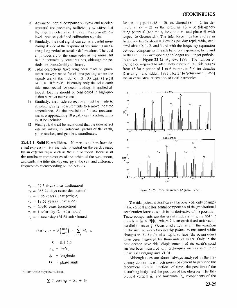
GEOKINETICS

8. Advanced inertial components (gyros and acceler- for the long period (S = 0), the diurnal (S = 1), the de-ometers) are becoming sufficiently sensitive that midiurnal (S = 2), or the terdiurnal (S = 3) tide-gener-the tides are detectable. They can thus provide low ating potential (at time t, longitude O, and phase O withlevel, precisely-defined calibration signals. respect to Greenwich). The tidal force thus has energy in

9. Similarly, the tidal signal can act as a useful mon- frequency bands about 0.3 cycles per day (cpd) wide, cen-itoring device of the response of instruments meas- tered about 0, 1, 2, and 3 cpd with the frequency separationuring long-period or secular deformations. The tidal between components in each band corresponding to T1 andamplitudes are of the same order as the annual tilt further splitting corresponding to longer and longer periods,rate in tectonically active regions, although the pe- as shown in Figure 23-25 [Agnew, 1979]. The number ofriods are considerably different. harmonics required to adequately represent the tide ranges

10. Tidal corrections have long been made to gravi- from 13 for a period of I to 6 months to 500 for decadesmeter surveys made for oil prospecting where the [Cartwright and Edden, 1973]. Refer to Schureman [1958]signals are of the order of 10-100 ugal (1 ugal for an exhaustive derivation of tidal harmonics.= I x 10-6 cm/s 2). Normally only the solid earthtide, uncorrected for ocean loading, is applied al-though loading should be considered in high-pre- DIURNAL

cision surveys near coasts.11. Similarly, earth tide corrections must be made to

absolute gravity measurements to remove the timedependence. As the precision of these measure-ments is approaching 10 ugal, ocean loading termsmust be included.

12. Finally, it should be mentioned that the tides affectsatellite orbits, the rotational period of the earth,polar motion, and geodetic coordinates. cpd

SEMIDIURNAL

23.4.2.1 Solid Earth Tides. Numerous authors have de-rived expressions for the tidal potential on the earth caused -by an exterior mass such as the sun or moon. Because of 2

the nonlinear complexities of the orbits of the sun, moon,and earth, the tides display energy at the sum and differencefrequencies corresponding to the periods

cpd

T1 = 27.3 days (lunar declination)T2 = 365.24 days (solar declination) Figure 23-25. Tidal harmonics [Agnew. 1979].

T3 = 8.85 years (lunar perigee)

T4 = 18.61 years (lunar node) The tidal potential itself cannot be observed, only changesT5 = 20940 years (perihelion) in the vertical and horizontal components of the gravitational

T0 = I solar day (24 solar hours) acceleration force g, which is the derivative of the potential.Tc = 1 lunar day (24.84 solar hours) These components are the gravity tides g = g · z and tilt

tides h = g x Zl/lgl, where z is an earth-fixed unit vector5 parallel to mean g. Occasionally tidal strain, the variation

that is, a = S wo) + E Mk Wk in distance between two nearby points, is measured whileWc k= 1 changes in the height of a liquid surface (the ocean tides)

have been measured for thousands of years. Only in theS = 0,1,2,3 past decade have tidal displacements of the earth's solid

Wk = 2pi/Tk surface been measured with techniques such as satellite orlunar laser ranging and VLBI.

m = longitude Although tides are almost always analyzed in the fre-0 = phase angle quency domain, it is much more convenient to generate the

theoretical tides as functions of time, the position of thein harmonic representation, disturbing body, and the position of the observer. The the-

oretical vertical gm and horizontal h,, components of theE Cj cos(ajt + Sa, + O)

23-25

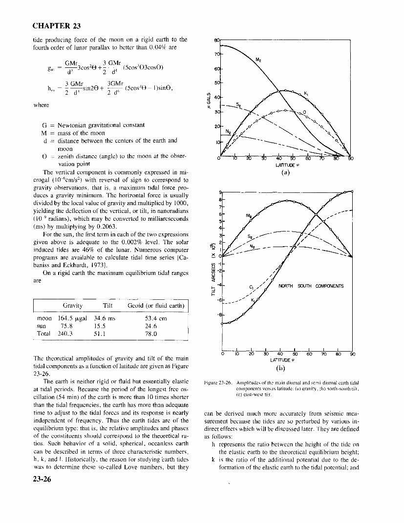
CHAPTER 23

tide producing force of the moon on a rigid earth to thefourth order of lunar parallax to better than 0.04% are

GMr 3 GMrgm = d3 3cos20 3/2+ - (5cos3 O3cosO) 6

3 GMr 3GMrhm - sin2O + 2 (5cos2 O- I)sinO,2 d3 2 d4

where

G = Newtonian gravitational constant 20M = mass of the moond = distance between the centers of the earth and

moon

0 = zenith distance (angle) to the moon at the obser- 0 ovation point LATITUE O

The vertical component is commonly expressed in mi- (a)crogal (10 6cm/s 2 ) with reversal of sign to correspond togravity observations, that is, a maximum tidal force pro-duces a gravity minimum. The horizontal force is usually 8divided by the local value of gravity and multiplied by 1000,yielding the deflection of the vertical, or tilt, in nanoradians 6

(10-9 radians), which may be converted to milliarcseconds(ms) by multiplying by 0.2063. 4

For the sun, the first term in each of the two expressions 3given above is adequate to the 0.002% level. The solar 2induced tides are 46% of the lunar. Numerous computer 1programs are available to calculate tidal time series [Ca- 0baniss and Eckhardt, 1973]. -1

On a rigid earth the maximum equilibrium tidal ranges -2are

-4 NORTH SOUTH COMPONENTS

-6Gravity Tilt Geoid (or fluid earth)

moon 164.5 ugal 34.6 ms 53.4 cmsun 75.8 15.5 24.6Total 240.3 51.1 78.0

0 10 20 30 40 50 60 70 80 90The theoretical amplitudes of gravity and tilt of the main LATITUDE p

tidal components as a function of latitude are given as Figure (b)23-26.

The earth is neither rigid or fluid but essentially elastic Figure 23-26. Amplitudes of the main diurnal and semi-diurnal earth tidal

at tidal periods. Because the period of the longest free os- components versus latitude: (a) gravity, (b) north-south tilt,

cillation (54 min) of the earth is more than 10 times shorter (c) east-west tilt.than the tidal frequencies, the earth has more than adequatetime to adjust to the tidal forces and its response is nearly can be derived much more accurately from seismic mea-independent of frequency. Thus the earth tides are of the surement because the tides are so perturbed by various in-equilibrium type; that is, the relative amplitudes and phases direct effects which will be discussed later. They are definedof the constituents should correspond to the theoretical ra- as follows:tios. Such behavior of a solid, spherical, oceanless earth h represents the ratio between the height of the tide oncan be described in terms of three characteristic numbers, the elastic earth to the theoretical equilibrium height;h, k, and l. Historically, the reason for studying earth tides k is the ratio of the additional potential due to the de-was to determine these so-called Love numbers, but they formation of the elastic earth to the tidal potential; and

23-26

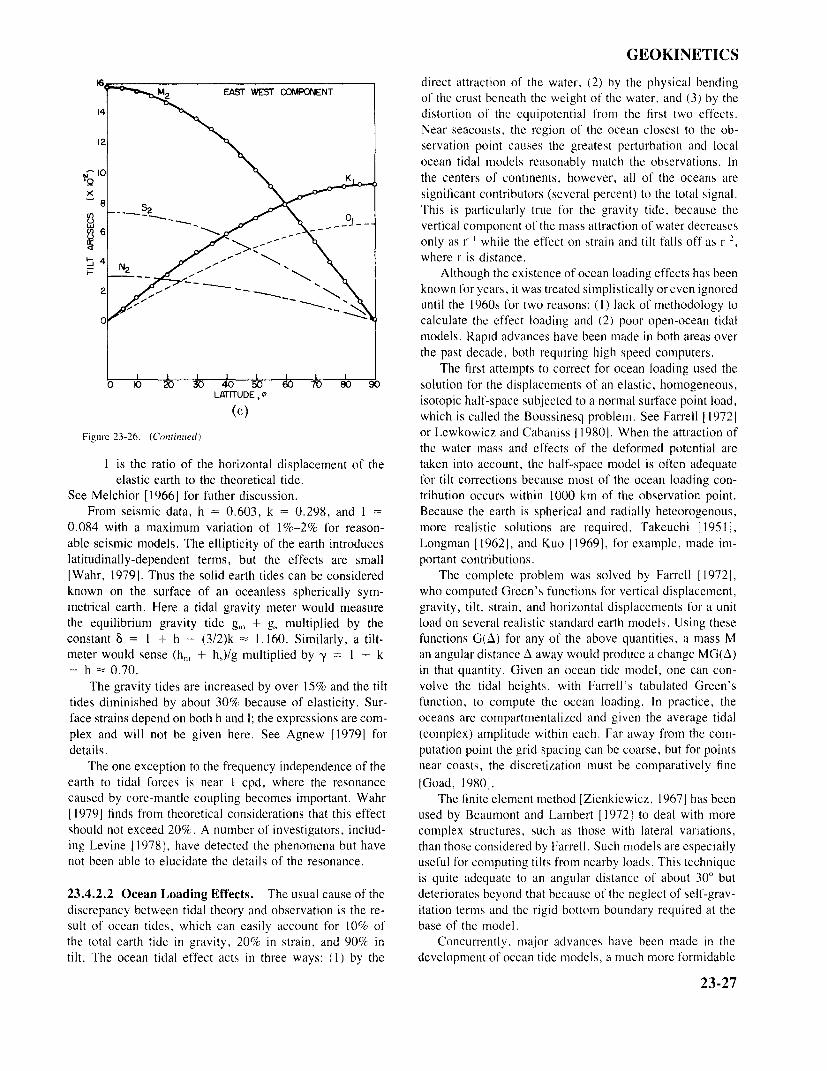
GEOKINETICS

EAST WEST COMPONENT direct attraction of the water, (2) by the physical bendingof the crust beneath the weight of the water, and (3) by thedistortion of the equipotential from the first two effects.Near seacoasts, the region of the ocean closest to the ob-

12 servation point causes the greatest perturbation and localocean tidal models reasonably match the observations. Inthe centers of continents, however, all of the oceans aresignificant contributors (several percent) to the total signal.This is particularly true for the gravity tide, because thevertical component of the mass attraction of water decreasesonly as r-l while the effect on strain and tilt falls off as r-2,

4 where r is distance.Although the existence of ocean loading effects has been

known for years, it was treated simplistically or even ignoreduntil the 1960s for two reasons: (1) lack of methodology tocalculate the effect loading and (2) poor open-ocean tidalmodels. Rapid advances have been made in both areas overthe past decade, both requiring high speed computers.

The first attempts to correct for ocean loading used the10 20 30 40 50 60 70 80 90 solution for the displacements of an elastic, homogeneous,

LATITUDE,P isotopic half-space subjected to a normal surface point load,(c) which is called the Boussinesq problem. See Farrell [19721

Figure 23-26. (Continued) or Lewkowicz and Cabaniss 11980]. When the attraction ofthe water mass and effects of the deformed potential are

l is the ratio of the horizontal displacement of the taken into account, the half-space model is often adequateelastic earth to the theoretical tide. for tilt corrections because most of the ocean loading con-

See Melchior [1966] for futher discussion. tribution occurs within 1000 km of the observation point.From seismic data, h = 0.603, k = 0.298, and I = Because the earth is spherical and radially heteorogenous,

0.084 with a maximum variation of 1%-2% for reason- more realistic solutions are required. Takeuchi [1951],able seismic models. The ellipticity of the earth introduces Longman [1962], and Kuo [1969], for example, made im-latitudinally-dependent terms, but the effects are small portant contributions.[Wahr, 1979]. Thus the solid earth tides can be considered The complete problem was solved by Farrell [1972],known on the surface of an oceanless spherically sym- who computed Green's functions for vertical displacement,metrical earth. Here a tidal gravity meter would measure gravity, tilt, strain, and horizontal displacements for a unitthe equilibrium gravity tide gm + gs multiplied by the load on several realistic standard earth models. Using theseconstant 8 = I + h - (3/2)k = 1.160. Similarly, a tilt- functions G(A) for any of the above quantities, a mass Mmeter would sense (h,,, + hs)/g multiplied by y = 1 + k an angular distance A away would produce a change MG(A)- h - 0.70. in that quantity. Given an ocean tide model, one can con-

The gravity tides are increased by over 15% and the tilt volve the tidal heights, with Farrell's tabulated Green'stides diminished by about 30% because of elasticity. Sur- function, to compute the ocean loading. In practice, theface strains depend on both h and l; the expressions are com- oceans are compartmentalized and given the average tidalplex and will not be given here. See Agnew [1979] for (complex) amplitude within each. Far away from the com-details. putation point the grid spacing can be coarse, but for points

The one exception to the frequency independence of the near coasts, the discretization must be comparatively fineearth to tidal forces is near l cpd, where the resonance [Goad, 1980].caused by core-mantle coupling becomes important. Wahr The finite element method [Zienkiewicz, 1967] has been[1979] finds from theoretical considerations that this effect used by Beaumont and Lambert [1972] to deal with moreshould not exceed 20%. A number of investigators, includ- complex structures, such as those with lateral variations,ing Levine 11978], have detected the phenomena but have than those considered by Farrell. Such models are especiallynot been able to elucidate the details of the resonance. useful for computing tilts from nearby loads. This technique

is quite adequate to an angular distance of about 30° but23.4.2.2 Ocean Loading Effects. The usual cause of the deteriorates beyond that because of the neglect of self-grav-discrepancy between tidal theory and observation is the re- itation terms and the rigid bottom boundary required at thesult of ocean tides, which can easily account for 10% of base of the model.the total earth tide in gravity, 20% in strain, and 9 0% in Concurrently. major advances have been made in thetilt. The ocean tidal effect acts in three ways: (1) by the development of ocean tide models, a much more formidable

23-27

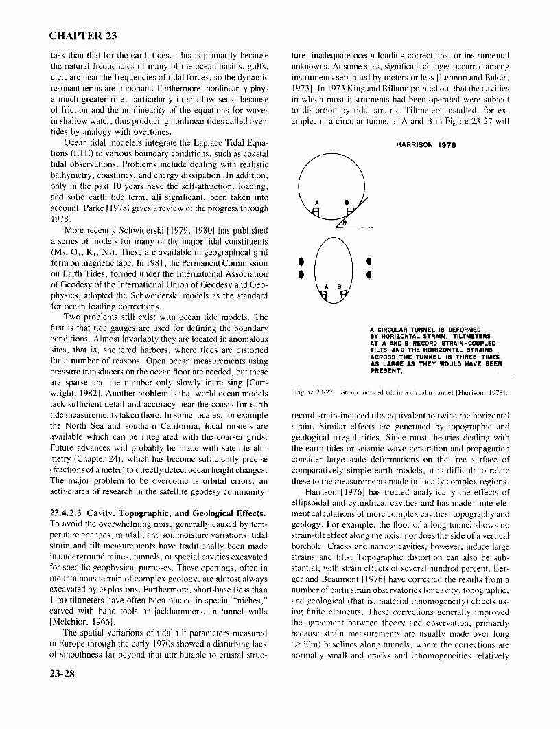
CHAPTER 23

task than that for the earth tides. This is primarily because ture, inadequate ocean loading corrections, or instrumentalthe natural frequencies of many of the ocean basins, gulfs, unknowns. At some sites, significant changes occurred amongetc., are near the frequencies of tidal forces, so the dynamic instruments separated by meters or less [Lennon and Baker,resonant terms are important. Furthermore, nonlinearity plays 1973]. In 1973 King and Bilham pointed out that the cavitiesa much greater role, particularly in shallow seas, because in which most instruments had been operated were subjectof friction and the nonlinearity of the equations for waves to distortion by tidal strains. Tiltmeters installed, for ex-in shallow water, thus producing nonlinear tides called over- ample, in a circular tunnel at A and B in Figure 23-27 willtides by analogy with overtones.

Ocean tidal modelers integrate the Laplace Tidal Equa- HARRISON 1978tions (LTE) to various boundary conditions, such as coastaltidal observations. Problems include dealing with realisticbathymetry, coastlines, and energy dissipation. In addition,only in the past 10 years have the self-attraction, loading,and solid earth tide term, all significant, been taken intoaccount. Parke 11978] gives a review of the progress through1978.

More recently Schwiderski [1979, 1980] has publisheda series of models for many of the major tidal constituents(M2, O1, K1, N2). These are available in geographical gridform on magnetic tape. In 1981, the Permanent Commissionon Earth Tides, formed under the International Associationof Geodesy of the International Union of Geodesy and Geo-physics, adopted the Schweiderski models as the standardfor ocean loading corrections.

Two problems still exist with ocean tide models. Thefirst is that tide gauges are used for defining the boundary A CIRCULAR TUNNEL IS DEFORMEDconditions. Almost invariably they are located in anomalous BY HORIZONTAL STRAIN. TILTMETERSAT A AND B RECORD STRAIN-COUPLEDsites, that is, sheltered harbors, where tides are distorted TILTS AND THE HORIZONTAL STRAINS

ACROSS THE TUNNEL IS THREE TIMESfor a number of reasons. Open ocean measurements using AS LARGE AS THEY WOULD HAVE BEENpressure transducers on the ocean floor are needed, but these PRESENT.are sparse and the number only slowly increasing [Cart-wright, 1982]. Another problem is that world ocean models Figure 23-27. Strain-induced tilt in a circular tunnel [Harrison, 19781.

lack sufficient detail and accuracy near the coasts for earthtide measurements taken there. In some locales, for example record strain-induced tilts equivalent to twice the horizontalthe North Sea and southern California, local models are strain. Similar effects are generated by topographic andavailable which can be integrated with the coarser grids. geological irregularities. Since most theories dealing withFuture advances will probably be made with satellite alti- the earth tides or seismic wave generation and propagationmetry (Chapter 24), which has become sufficiently precise consider large-scale deformations on the free surface of(fractions of a meter) to directly detect ocean height changes. comparatively simple earth models, it is difficult to relateThe major problem to be overcome is orbital errors, an these to the measurements made in locally complex regions.active area of research in the satellite geodesy community. Harrison [1976] has treated analytically the effects of

ellipsoidal and cylindrical cavities and has made finite ele-23.4.2.3 Cavity, Topographic, and Geological Effects. ment calculations of more complex cavities, topography andTo avoid the overwhelming noise generally caused by tem- geology. For example, the floor of a long tunnel shows noperature changes, rainfall, and soil moisture variations, tidal strain-tilt effect along the axis, nor does the side of a verticalstrain and tilt measurements have traditionally been made borehole. Cracks and narrow cavities, however, induce largein underground mines, tunnels, or special cavities excavated strains and tilts. Topographic distortion can also be sub-for specific geophysical purposes. These openings, often in stantial, with strain effects of several hundred percent. Ber-mountainous terrain of complex geology, are almost always ger and Beaumont [1976] have corrected the results from aexcavated by explosions. Furthermore, short-base (less than number of earth strain observatories for cavity, topographic,1 m) tiltmeters have often been placed in special "niches," and geological (that is, material inhomogeneity) effects us-carved with hand tools or jackhammers, in tunnel walls ing finite elements. These corrections generally improved[Melchior, 1966]. the agreement between theory and observation, primarily

The spatial variations of tidal tilt parameters measured because strain measurements are usually made over longin Europe through the early 1970s showed a disturbing lack '>30m) baselines along tunnels, where the corrections areof smoothness far beyond that attributable to crustal struc- normally small and cracks and inhomogeneities relatively

23-28

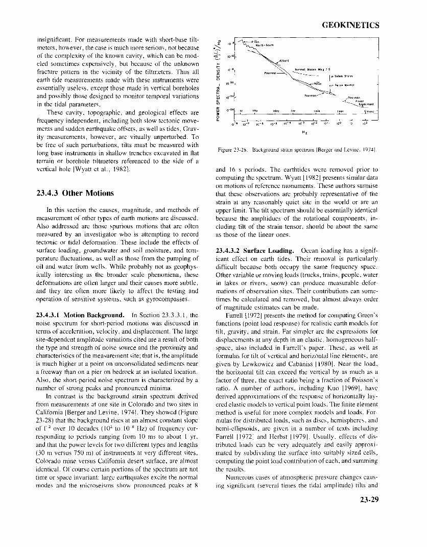
GEOKINETICS

insignificant. For measurements made with short-base tilt-meters, however, the case is much more serious, not becauseof the complexity of the known cavity, which can be mod-eled sometimes expensively, but because of the unknownfracture pattern in the vicinity of the tiltmeters. Thus allearth tide measurements made with these instruments wereessentially useless, except those made in vertical boreholesand possibly those designed to monitor temporal variationsin the tidal parameters.

These cavity, topographic, and geological effects arefrequency independent, including both slow tectonic move- 0-

ments and sudden earthquake offsets, as well as tides. Grav-ity measurements, however, are vitually unperturbed. Tobe free of such perturbations, tilts must be measured with

Figure 23-28. Background strain spectrum [Berger and Levine, 1974].long base instruments in shallow trenches excavated in flatterrain or borehole tiltmeters referenced to the side of avertical hole [Wyatt et al., 1982]. and 16 s periods. The earthtides were removed prior to

computing the spectrum. Wyatt 119821 presents similar dataon motions of reference monuments. These authors surmise

23.4.3 Other Motions that these observations are probably representative of thestrain at any reasonably quiet site in the world or are an

In this section the causes, magnitude, and methods of upper limit. The tilt spectrum should be essentially identicalmeasurement of other types of earth motions are discussed. because the ampltidues of the rotational components, in-Also addressed are those spurious motions that are often cluding tilt of the strain tensor, should be about the samemeasured by an investigator who is attempting to record as those of the linear ones.tectonic or tidal deformation. These include the effects ofsurface loading, groundwater and soil moisture, and tem- 23.4.3.2 Surface Loading. Ocean loading has a signif-perature fluctuations, as well as those from the pumping of icant effect on earth tides. Their removal is particularlyoil and water from wells. While probably not as geophys- difficult because both occupy the same frequency space.ically interesting as the broader scale phenomena, these Other variable or moving loads (trucks, trains, people, waterdeformations are often larger and their causes more subtle, in lakes or rivers, snow) can produce measurable defor-and they are often more likely to affect the testing and mations of observation sites. Their contributions can some-operation of sensitive systems, such as gyrocompasses. times be calculated and removed, but almost always order

of magnitude estimates can be made.23.4.3.1 Motion Background. In Section 23.3.3.1, the Farrell [1972] presents the method for computing Green'snoise spectrum for short-period motions was discussed in functions (point load response) for realistic earth models forterms of acceleration, velocity, and displacement. The large tilt, gravity, and strain. Far simpler are the expressions forsite-dependent amplitude variations cited are a result of both displacements at any depth in an elastic, homogeneous half-the type and strength of noise source and the proximity and space, also included in Farrell's paper. These, as well ascharacteristics of the measurement site; that is, the amplitude formulas for tilt of vertical and horizontal line elements, areis much higher at a point on unconsolidated sediments near given by Lewkowicz and Cabaniss 11980]. Near the load,a freeway than on a pier on bedrock at an isolated location. the horizontal tilt can exceed the vertical by as much as aAlso, the short-period noise spectrum is characterized by a factor of three, the exact ratio being a fraction of Poisson'snumber of strong peaks and pronounced minima. ratio. A number of authors, including Kuo [1969], have

In contrast is the background strain spectrum derived derived approximations of the response of horizontally lay-from measurements at one site in Colorado and two sites in ered elastic models to vertical point loads. The finite elementCalifornia [Berger and Levine, 1974]. They showed (Figure method is useful for more complex models and loads. For-23-28) that the background rises at an almost constant slope mulas for distributed loads, such as discs, hemispheres, andof f 2 over 10 decades (102 to 10 Hz) of frequency cor- hemi-ellipsoids, are given in a number of texts includingresponding to periods ranging from 10 ms to about 1 yr, Farrell [1972] and Herbst 11979]. Usually, effects of dis-and that the power levels for two different types and lengths tributed loads can be very adequately and easily approxi-(30 m versus 750 m) of instruments at very different sites, mated by subdividing the surface into suitably sized cells,Colorado mine versus California desert surface, are almost computing the point load contribution of each, and summingidentical. Of course certain portions of the spectrum are not the results.time or space invariant: large earthquakes excite the normal Numerous cases of atmospheric pressure changes caus-modes and the microseisms show pronounced peaks at 8 ing significant (several times the tidal amplitude) tilts and

23-29

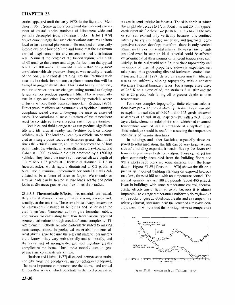
CHAPTER 23

strains appeared until the early 1970s in the literature [Mel- waves in semi-infinite halfspaces. The skin depth at whichchior, 1966]. Some authors postulated the coherent move- the amplitude decays to l/e is about I m and 20 m in typicalment of crustal blocks hundreds of kilometers wide and earth materials for these two periods. In this model the rockpartially decoupled from adjoining blocks. Herbst 11979] or soil can expand only vertically because it is confinedargues convincingly that such observations must result from laterally by equally heated materials, and horizontal com-local or instrumental phenomena. He modeled an unusually pressive stresses develop; therefore, there is only verticalintense cyclonic low of 50 mb and found that the maximum strain, no tilts or horizontal strains. However, instrumentsvertical displacement for any reasonable load distribution installed even in such an ideal material could be affectedwas 16 mm at the center of the loaded region, with a tilt by asymmetry of their mounts or inherent temperature sen-of 45 nrads at the center and edge, far less than the typical sitivity. In the real world with finite surface topography andtidal tilt of 100 nrads. He was able to show that the apparent variations of thermal properties, sideways expansion cancorrelation with air pressure changes was actually a result take place, thus generating tilts and horizontal strains. Har-of the concurrent rainfall draining into the fractured rock rison and Herbst [1977] derive an expression for tilts andnear his borehole instruments, a phenomenon that will be strains on uniformly sloping topography with a constanttreated in greater detail later. This is not to say, of course, thickness thermal boundary layer. For a temperature wavethat air or water pressure changes acting normal to sloping of 283 K on a slope of 6° , the strain is 2 x 10-6 and theterrain cannot produce significant tilts. This is especially tilt is 20 urads, both falling off at greater depths as doestrue in clays and other low-permeability materials where temperature.diffusion of pore fluids becomes important [Zschau, 1976]. For more complex topography, finite element calcula-Direct pressure effects on instruments act by either distorting tions have proved quite satisfactory. Herbst [1979] was ablecompliant sealed cases or buoying the mass in unsealed to explain annual tilts of 0.625 and 0.125 urads observedcases. The variations of mass attraction of the atmosphere at depths of 15 and 30 m, respectively, with a 2-D, three-must be considered in very precise earth tide gravimetry. layer, finite element model of this site, which had an annual

Vehicles and fluid storage tanks can produce significant temperature wave of 281 K amplitude at a depth of 1 m.tilts and tilt rates at nearby test facilities built on uncon- This technique should be useful in assessing the temperaturesolidated soils. The load produced by a vehicle can be mod- sensitivity of various structures.eled as a single point source at distances greater than three In buildings and other facilities, especially those ex-times the vehicle diameter, and as the superposition of four posed to solar insolation, the tilts can be very large. As onepoint loads, the wheels, at lesser distances. Lewkowicz and side of a building expands, it bends, flexing the floors andCabaniss 11980] examined the tilts produced by a 1500 kg transmitting stresses to its foundation. These can affect testvehicle. They found the maximum vertical tilt at a depth of piers completely decoupled from the building floors and1.3 m was 1.25 urads at a horizontal distance of 1.3 m walls unless such piers are some distance from the foun-(nearest axle), which rapidly diminished to 0.2 urads at dation. Figure 23-29 [Tsutsumi, 1970] shows the tilt on a6 m. The maximum, unmeasured horizontal tilt was cal- pier in an insulated building standing on exposed bedrockculated to be a factor of three or larger. Water tanks or on a low, forested hill and with no temperature control. Thesimilar loads can be treated as disc loads nearby and point annual variation is over 100 arcseconds (about 485 urads).loads at distances greater than five times their radius. Even in buildings with some temperature control, thermo-

elastic effects are difficult to avoid because it is almost23.4.3.3 Thermoelastic Effects. As materials are heated, impossible to change temperatures uniformly throughout anthey almost always expand, thus producing stresses and, entire room. Figure 23-30 shows the tilts and air temperatureusually, strains and tilts. These are almost always observable (clearly diurnal) measured near the center of a massive con-on instruments installed in buildings and on or near the crete pier. First, note that the phasing between temperatureearth's surface. Numerous authors give formulas, tables,and curves for calculating heat flow from various types ofsource distributions through media of some complexity. Fi- NORTH-SOUH TILT

nite element methods are also particularly suited to making WESTON, MASS 1966-1968

such computations. In geological materials, problems al- 25 SEC

most always arise because the relevant material parametersare unknown: they vary both spatially and temporally, andthe movement of groundwater and soil moisture greatly EAST-WEST TILT

complicates the issue. Thus, most models used in geo- WESTON, MASS

physics are comparatively simple.Harrison and Herbst [1977] discussed thermoelastic strains

0 A 0and tilts from the geophysical instrumentation standpoint. TIME MONTHS)

The most important components are the diurnal and annualtemperature waves, which penetrate as damped progressive Figure 23-29. Weston vault tilt [Tsutsumi. 1970].

23-30

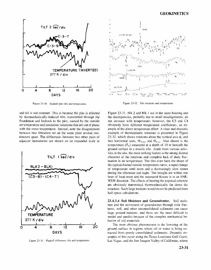
GEOKINETICS

TILT 2 sec/div

SCC RMAD

TEMPERATURE (INVERTED) LCD OPEN

277 K / div

0 4 8 12 16 20DAYS

Figure 23-30. Haskell pier tilts and temperature. Figure 23-32. Silo rotations and temperature.

and tilt is not constant. This is because the pier is affected Figure 23-31. Blk 2 and Blk 1 are in the same housing andby thermoelastically-induced tilts, transmitted through the the discrepancies, probably due to small misalignments, dofoundation and bedrock to the pier, caused by the outside not increase with temperature; however, the C3 and C4air temperature and insolation variations that are out of phase obviously have different temperature coefficients, an ex-with the room temperature. Second, note the disagreement ample of the direct temperature effect. A clear and dramaticbetween two tiltmeters set on the same plate several cen- example of thermoelastic rotations is presented in Figuretimeters apart. The differences between two other pairs of 23-32, which shows rotations about the vertical axis Oz andadjacent instruments are shown on an expanded scale in two horizontal axes, ONorth and OEast. Also shown is the

temperature (TB) measured at a depth of 10 m beneath theground surface in a missile silo. Aside from various activ-ities in the silo, the most striking feature is the strong diurnal

TILT I sec/div character of the rotations and complete lack of daily fluc-tuation in air temperature. The tilts even have the shape of

BLK2 - BLKI the typical diurnal outside temperature curve, a rapid changeFigure_23-30. of temperature until noon and a decreasingly slow return

during the afternoon and night. The troughs are within one(C3 -8)- (C4- 7 ) hour of local noon and the measured flexure is in an ENE-

WSW direction. The effects of heating the exposed concreteare obviously transmitted thermoelastically far down thestructure. Such large motions would never be predicted fromhalf-space calculations.

23.4.3.4 Soil Moisture and Groundwater. Soil mois-ture and the movement of groundwater through rock frac-tures, soil, and other unconsolidated sediments can cause

TEMPERATURE large ground motions, and these are the most difficult tomodel and predict because of the complex mechanical be-

277 K/div havior of soil materials.

The most obvious phenomenon is the lowering of theground surface in regions where oil or water is being ex-

DAYS tracted from poorly consolidated sediments. Dramatic ex-amples of this occur along the Texas-Louisiana Gulf Coast,

Figure 23-31. Haskell difference tilts and temperature. Las Vegas, and the San Joaquin Valley of California, where

23-31

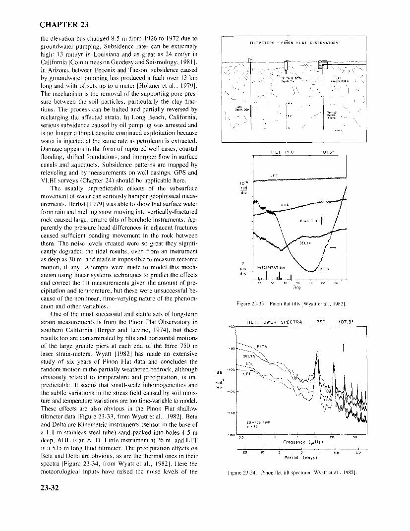
CHAPTER 23

the elevation has changed 8.5 m from 1926 to 1972 due togroundwater pumping. Subsidence rates can be extremely TILTMETERS - PINON FLAT OBSERVATORY

high: 13 mm/yr in Louisiana and as great as 24 cm/yr inCalifornia [Committees on Geodesy and Seismology, 1981].In Arizona, between Phoenix and Tucson, subsidence causedby groundwater pumping has produced a fault over 13 kmlong and with offsets up to a meter [Holzner et al., 1979].The mechanism is the removal of the supporting pore pres-sure between the soil particles, particularly the clay frac-tions. The process can be halted and partially reversed byrecharging the affected strata. In Long Beach, California,serious subsidence caused by oil pumping was arrested andis no longer a threat despite continued exploitation becausewater is injected at the same rate as petroleum is extracted.Damage appears in the form of ruptured well cases, coastal TILT PFO 107.3°

flooding, shifted foundations, and improper flow in surfacecanals and aqueducts. Subsidence patterns are mapped byreleveling and by measurements on well casings. GPS and LFT

VLBI surveys (Chapter 24) should be applicable here.The usually unpredictable effects of the subsurface

movement of water can seriously hamper geophysical meas-urements. Herbst 11979] was able to show that surface water ADL

from rain and melting snow moving into vertically-fracturedrock caused large, erratic tilts of borehole instruments. Ap- Down Tilt

parently the pressure head differences in adjacent fracturescaused sufficient bending movement in the rock betweenthem. The noise levels created were so great they signifi- DELT

cantly degraded the tidal results, even from an instrumentas deep as 30 m, and made it impossible to measure tectonicmotion, if any. Attempts were made to model this mech- cm PRECIPITATION BETA

anism using linear systems techniques to predict the effects div

and correct the tilt measurements given the amount of pre-cipitation and temperature, but these were unsuccessful be- Day

cause of the nonlinear, time-varying nature of the phenom-Figure 23-33. Pinon f1at tilts [Wyatt et al., 1982].enon and other variables.

One of the most successful and stable sets of long-termstrain measurements is from the Pinon Flat Observatory in TILT POWER SPECTRA PFO 107.3o

southern California [Berger and Levine, 1974], but theseresults too are contaminated by tilts and horizontal motionsof the large granite piers at each end of the three 750 m -80

laser strain-meters. Wyatt [1982] has made an extensive DEELAstudy of six years of Pinon Flat data and concludes the ADL

random motion in the partially weathered bedrock, althoughobviously related to temperature and precipitation, is un-predictable. It seems that small-scale inhomogeneities andthe subtle variations in the stress field caused by soil mois-ture and temperature variations are too time-variable to model.These effects are also obvious in the Pinon Flat shallowtiltmeter data [Figure 23-33, from Wyatt et al., 19821. Betaand Delta are Kinemetric instruments (sensor in the base ofa 1.1 m stainless steel tube) sand-packed into holes 4.5 m

0.5 20 50deep, ADL is an A. D. Little instrument at 26 m, and LFT Frequency (uHz)is a 535 m long fluid tiltmeter. The precipitation effects on

5Beta and Delta are obvious, as are the thermal ones in their Period (days)

spectra [Figure 23-34, from Wyatt et al., 1982]. Here themeteorological inputs have raised the noise levels of the Figure 23-34. Pinon flat tilt spectrum [Wyatt et al., 1982].

23-32

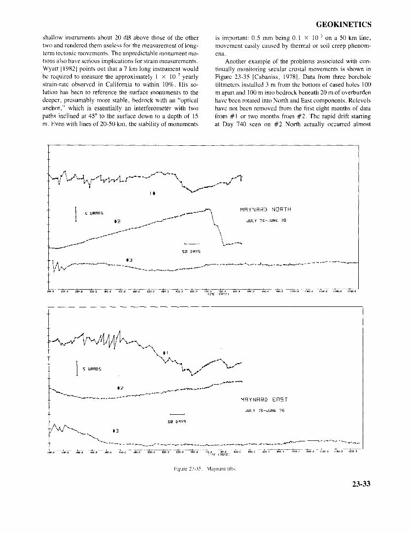
GEOKINETICS

shallow instruments about 20 dB above those of the other is important: 0.5 mm being 0.1 x 10-7 on a 50 km line,two and rendered them useless for the measurement of long- movement easily caused by thermal or soil creep phenom-term tectonic movements. The unpredictable monument mo- ena.tions also have serious implications for strain measurements. Another example of the problems associated with con-Wyatt [1982] points out that a 7 km long instrument would tinually monitoring secular crustal movements is shown inbe required to measure the approximately 1 x 10-7 yearly Figure 23-35 [Cabaniss, 1978]. Data from three boreholestrain-rate observed in California to within 10%. His so- tiltmeters installed 3 m from the bottom of cased holes 100lution has been to reference the surface monuments to the m apart and 100 m into bedrock beneath 20 m of overburdendeeper, presumably more stable, bedrock with an "optical have been rotated into North and East components. Relevelsanchor," which is essentially an interferometer with two have not been removed from the first eight months of datapaths inclined at 45° to the surface down to a depth of 15 from #1 or two months from #2. The rapid drift startingm. Even with lines of 20-50 km, the stability of monuments at Day 740 seen on #2 North actually occurred almost

5 MYNRD NORTH

JULY 7-JUNE 78

TIME [DAYS]

URRDS

MAYNARD EAST

JULY 75-JUNE 78

TIME [DAYS)

Figure 23-35. Maynard tilts.

23-33

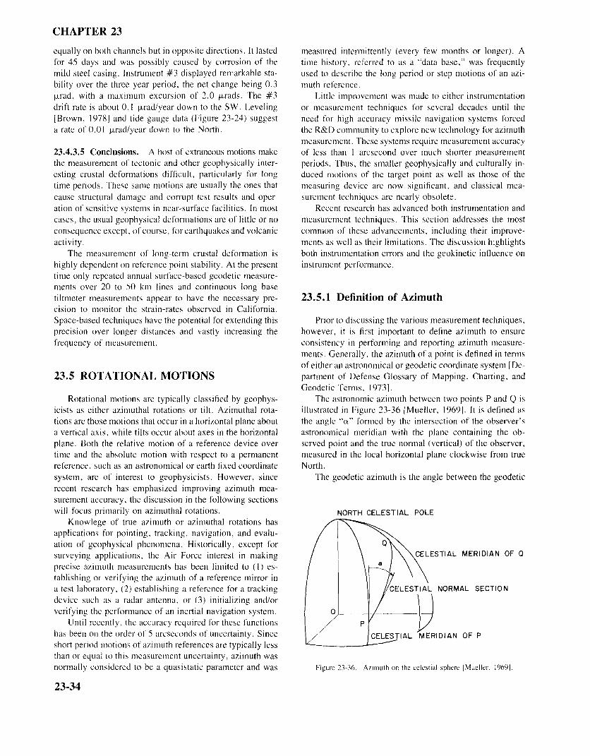
CHAPTER 23

equally on both channels but in opposite directions. It lasted measured intermittently (every few months or longer). Afor 45 days and was possibly caused by corrosion of the time history, referred to as a "data base," was frequentlymild steel casing. Instrument #3 displayed remarkable sta- used to describe the long period or step motions of an azi-bility over the three year period, the net change being 0.3 muth reference.urad, with a maximum excursion of 2.0 urads. The #3 Little improvement was made to either instrumentationdrift rate is about 0. I urad/year down to the SW. Leveling or measurement techniques for several decades until the[Brown, 1978] and tide gauge data (Figure 23-24) suggest need for high accuracy missile navigation systems forceda rate of 0.01 urad/year down to the North. the R&D community to explore new technology for azimuth

measurement. These systems require measurement accuracy23.4.3.5 Conclusions. A host of extraneous motions make of less than I arcsecond over much shorter measurementthe measurement of tectonic and other geophysically inter- periods. Thus, the smaller geophysically and culturally in-esting crustal deformations difficult, particularly for long duced motions of the target point as well as those of thetime periods. These same motions are usually the ones that measuring device are now significant, and classical mea-cause structural damage and corrupt test results and oper- surement techniques are nearly obsolete.ation of sensitive systems in near-surface facilities. In most Recent research has advanced both instrumentation andcases, the usual geophysical deformations are of little or no measurement techniques. This section addresses the mostconsequence except, of course, for earthquakes and volcanic common of these advancements, including their improve-activity. ments as well as their limitations. The discussion highlights

The measurement of long-term crustal deformation is both instrumentation errors and the geokinetic influence onhighly dependent on reference point stability. At the present instrument performance.time only repeated annual surface-based geodetic measure-ments over 20 to 50 km lines and continuous long basetiltmeter measurements appear to have the necessary pre- 23.5.1 Definition of Azimuthcision to monitor the strain-rates observed in California.Space-based techniques have the potential for extending this Prior to discussing the various measurement techniques,precision over longer distances and vastly increasing the however, it is first important to define azimuth to ensurefrequency of measurement. consistency in performing and reporting azimuth measure-

ments. Generally, the azimuth of a point is defined in termsof either an astronomical or geodetic coordinate system [De-

23.5 ROTATIONAL MOTIONS partment of Defense Glossary of Mapping, Charting, andGeodetic Terms, 1973].

Rotational motions are typically classified by geophys- The astronomic azimuth between two points P and Q isicists as either azimuthal rotations or tilt. Azimuthal rota- illustrated in Figure 23-36 [Mueller, 19691. It is defined astions are those motions that occur in a horizontal plane about the angle "a" formed by the intersection of the observer'sa vertical axis, while tilts occur about axes in the horizontal astronomical meridian with the plane containing the ob-plane. Both the relative motion of a reference device over served point and the true normal (vertical) of the observer,time and the absolute motion with respect to a permanent measured in the local horizontal plane clockwise from truereference, such as an astronomical or earth fixed coordinate North.system, are of interest to geophysicists. However, since The geodetic azimuth is the angle between the geodeticrecent research has emphasized improving azimuth mea-surement accuracy, the discussion in the following sectionswill focus primarily on azimuthal rotations. NORTH CELESTIAL POLE

Knowlege of true azimuth or azimuthal rotations hasapplications for pointing, tracking, navigation, and evalu-ation of geophysical phenomena. Historically, except forsurveying applications, the Air Force interest in making CELESTIAL MERIDIAN OF Qprecise azimuth measurements has been limited to (1) es-tablishing or verifying the azimuth of a reference mirror ina test laboratory, (2) establishing a reference for a tracking CELESTIAL NORMAL SECTIONdevice such as a radar antenna, or (3) initializing and/orverifying the performance of an inertial navigation system.

Until recently, the accuracy required for these functionshas been on the order of 5 arcseconds of uncertainty. Since CELESTIAL MERIDIAN OF Pshort period motions of azimuth references are typically lessthan or equal to this measurement uncertainty, azimuth wasnormally considered to be a quasistatic parameter and was Figure 23-36. Azimuth on the celestial sphere [Mueller, 19691.

23-34

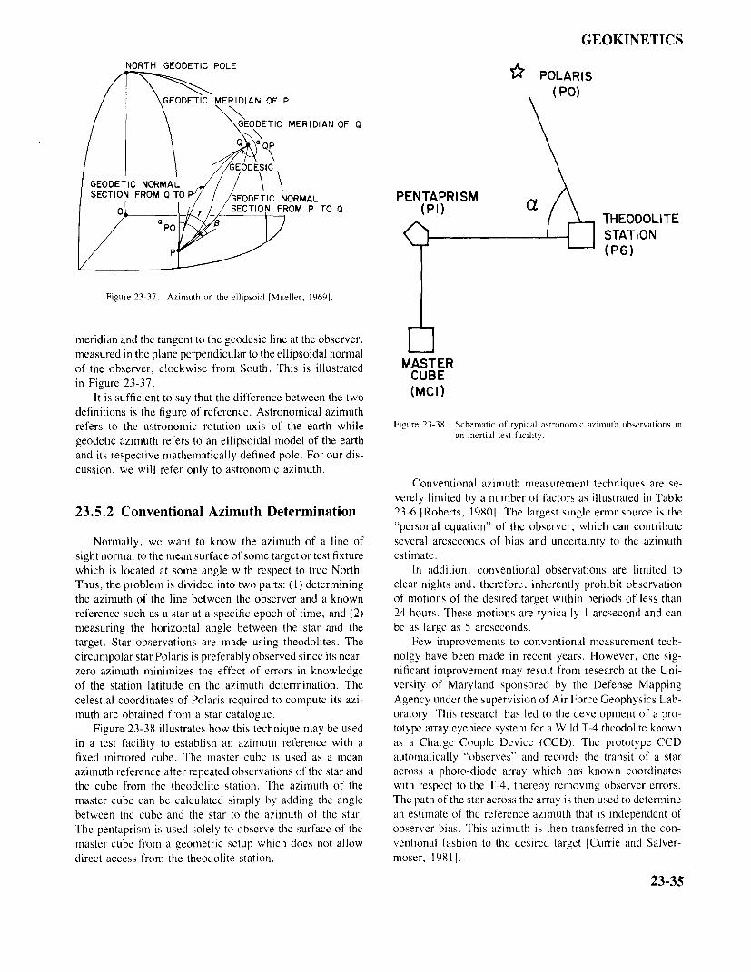
GEOKINETICS

NORTH GEODETIC POLEPOLARIS

GEODETIC MERIDIAN OF P

GEODETIC MERIDIAN OF Q

Q

GEODESIC

GEODETIC NORMALSECTION FROM Q TO P GEODETIC NORMAL PENTAPRISM

SECTION FROM P TO Q (P1) THEODOLITEPQ

STATION(P6)

Figure 23-37. Azimuth on the ellipsoid [Mueller, 1969].

meridian and the tangent to the geodesic line at the observer,measured in the plane perpendicular to the ellipsoidal normalof the observer, clockwise from South. This is illustrated MASTERin Figure 23-37.

It is sufficient to say that the difference between the two (MCI)definitions is the figure of reference. Astronomical azimuthrefers to the astronomic rotation axis of the earth while Figure 23-38. Schematic of typical astronomic azimuth observations in

geodetic azimuth refers to an ellipsoidal model of the earth an inertial test facility.and its respective mathematically defined pole. For our dis-cussion, we will refer only to astronomic azimuth.

Conventional azimuth measurement techniques are se-verely limited by a number of factors as illustrated in Table

23.5.2 Conventional Azimuth Determination 23-6 [Roberts, 19801. The largest single error source is the"personal equation" of the observer, which can contribute

Normally, we want to know the azimuth of a line of several arcseconds of bias and uncertainty to the azimuthsight normal to the mean surface of some target or test fixture estimate.which is located at some angle with respect to true North. In addition, conventional observations are limited toThus, the problem is divided into two parts: (1) determining clear nights and, therefore, inherently prohibit observationthe azimuth of the line between the observer and a known of motions of the desired target within periods of less thanreference such as a star at a specific epoch of time, and (2) 24 hours. These motions are typically 1 arcsecond and canmeasuring the horizontal angle between the star and the be as large as 5 arcseconds.target. Star observations are made using theodolites. The Few improvements to conventional measurement tech-circumpolar star Polaris is preferably observed since its near- nolgy have been made in recent years. However, one sig-zero azimuth minimizes the effect of errors in knowledge nificant improvement may result from research at the Uni-of the station latitude on the azimuth determination. The versity of Maryland sponsored by the Defense Mappingcelestial coordinates of Polaris required to compute its azi- Agency under the supervision of Air Force Geophysics Lab-muth are obtained from a star catalogue. oratory. This research has led to the development of a pro-

Figure 23-38 illustrates how this technique may be used totype array eyepiece system for a Wild T-4 theodolite knownin a test facility to establish an azimuth reference with a as a Charge Couple Device (CCD). The prototype CCDfixed mirrored cube. The master cube is used as a mean automatically "observes" and records the transit of a starazimuth reference after repeated observations of the star and across a photo-diode array which has known coordinatesthe cube from the theodolite station. The azimuth of the with respect to the T-4, thereby removing observer errors.master cube can be calculated simply by adding the angle The path of the star across the array is then used to determinebetween the cube and the star to the azimuth of the star. an estimate of the reference azimuth that is independent ofThe pentaprism is used solely to observe the surface of the observer bias. This azimuth is then transferred in the con-master cube from a geometric setup which does not allow ventional fashion to the desired target [Currie and Salver-direct access from the theodolite station. moser, 19811.

23-35

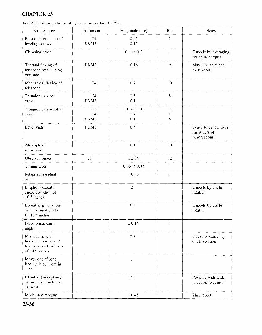
CHAPTER 23

Table 23-6. Azimuth or horizontal angle error sources [Roberts, 1980].

Error Source Instrument Magnitude (sec) Ref Notes

Elastic deformation of T4 0.05 8leveling screws DKM3 0.15

Clamping error 0.1 to 0.2 1 Cancels by averagingfor equal torques

Thermal flexing of DKM3 0.16 9 May tend to canceltelescope by touching by reversalone side

Mechanical flexing of T4 0.7 10telescope

Trunnion axis roll T4 0.6 8error DKM3 0.1

Trunnion axis wobble T3- 1 to +0.5 11error T4 0.4 8

DKM3 0.1 8

Level vials DKM3 0.5 1 Tends to cancel overmany sets ofobservations

Atmospheric 0.1 10refraction

Observer biases T3 + 2.84 12

Timing error 0.06 to 0.15

Petaprism residual ±0.25

error

Elliptic horizontal 2 Cancels by circlecircle distortion of rotation10-4 inches

Eccentric graduations 0.4 Cancels by circleon horizontal circle rotationby 10-4 inches

Porro prism can't +0.14angle

Misalignment of 0.4 Does not cancel byhorizontal circle and circle rotationtelescope vertical axesof 10- 4 inches

Movement of longline mark by I cm inI nm

Blunder. (Acceptance 0.3 Possible with wideof one 5 s blunder in rejection tolerance16 sets)

Model assumptions ± 0.45 This report

23-36

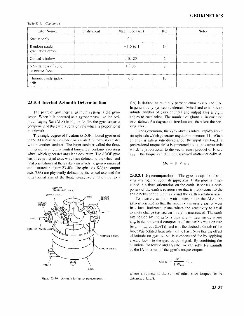
GEOKINETICS

Table 23-6. (Continued)

Error Source Instrument Magnitude (sec) Ref Notes

Star Models 0.1

Random circle -1.5 to 1 13graduation errors

Optical window +0.125 2

Non-flatness of cube +0.06 2or mirror faces

Thermal circle index 0.3 10drift

23.5.3 Inertial Azimuth Determination (1A) is defined as mutually perpendicular to SA and OA.In general, any gyroscopic element (wheel and axle) has an

The heart of any inertial azimuth system is the gyro- infinite number of pairs of input and output axes at rightscope. When it is operated as a gyrocompass like the Azi- angles to each other. The number of gimbals, in our casemuth Laying Set (ALS) in Figure 23-39, the gyro senses a two, defines the degrees of freedom and therefore the sen-component of the earth's rotation rate which is proportional sing axes.to azimuth. During operation, the gyro wheel is rotated rapidly about

The single degree of freedom (SDOF) floated gyro used the spin axis which generates angular momentum (H). Whenin the ALS may be described as a sealed cylindrical canister an angular rate is introduced about the input axis (wIA), awithin another canister. The inner canister called the float, precessional torque (Mo) is generated about the output axisimmersed in a fluid at neutral buoyancy, contains a rotating which is proportional to the vector cross product of H andwheel which generates angular momentum. The SDOF gyro (wIA. This torque can then be expressed mathematically ashas three principal axes which are defined by the wheel andfloat orientation and the gimbals on which the gyro is mounted Mo = H x WIA

as illustrated in Figure 23-40a. The spin axis (SA) and outputaxis (OA) are physically defined by the wheel axis and thelongitudinal axis of the float, respectively. The input axis 23.5.3.1 Gyrocompassing. The gyro is capable of sen-

sing any rotation about its input axis. If the gyro is main-tained in a fixed orientation on the earth, it senses a com-

AZIMUTHGIMBAL AXIS ponent of the earth's rotation rate that is proportional to the

BUBBLE LEVEL angle between the input axis and the earth's rotation axis.GYRO SENSOR MIRROR To measure azimuth with a sensor like the ALS, the

SENSOR MIRROR gyro is oriented so that the input axis is nearly east or westin a local horizontal plane where the sensitivity to smallazimuth change (sensed earth rate) is maximized. The earthrate sensed by the gyro is then WIA = WEH sin a, where

wEH is the horizontal component of the earth's rotation rate[WEH = wE cos (LAT)], and a is the desired azimuth of the

ROTATION GIMBAL AX,input axis defined from astronomic East. Note that the effect

ROTATION GIMBAL of latitude on gyro output is compensated for by applyinga scale factor to the gyro output signal. By combining theequations for torque and lA rate, we can solve for azimuth

AZIMUTH GIMBAL of the IA in terms of the gyro's torque output:

Mosin a =

TRIVET HW EHBASE

where E represents the sum of other error torques (to beFigure 23-39. Azimuth laying set gyrocompass. discussed later).

23-37

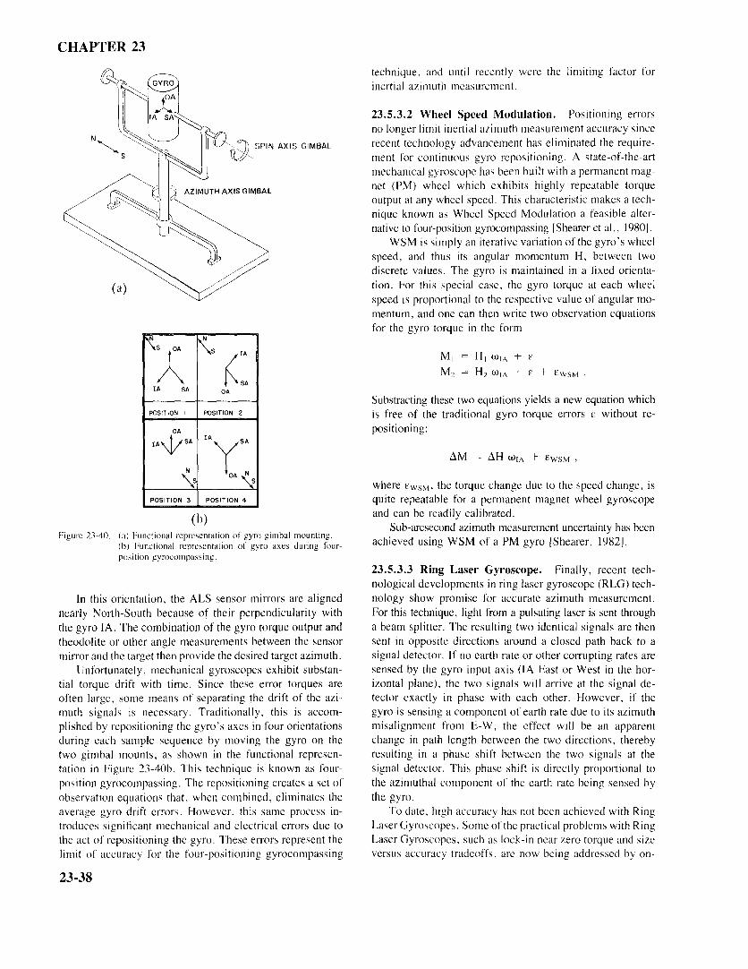
CHAPTER 23

technique, and until recently were the limiting factor forinertial azimuth measurement.

23.5.3.2 Wheel Speed Modulation. Positioning errorsno longer limit inertial azimuth measurement accuracy since

SPIN AXIS GIMBAL recent technology advancement has eliminated the require-ment for continuous gyro repositioning. A state-of-the-artmechanical gyroscope has been built with a permanent mag-

AZIMUTH AXIS GIMBAL net (PM) wheel which exhibits highly repeatable torqueoutput at any wheel speed. This characteristic makes a tech-nique known as Wheel Speed Modulation a feasible alter-native to four-position gyrocompassing [Shearer et al., 1980].

WSM is simply an iterative variation of the gyro's wheelspeed, and thus its angular momentum H, between twodiscrete values. The gyro is maintained in a fixed orienta-

(a) tion. For this special case, the gyro torque at each wheelspeed is proportional to the respective value of angular mo-mentum, and one can then write two observation equationsfor the gyro torque in the form

M1 H1 W1A + E

M2 = H2 -w1A + E + EwSM

Substracting these two equations yields a new equation whichPOSITION I POSITION 2 is free of the traditional gyro torque errors E without re-

positioning:

AM = AH w1A + EWSM,

where EWSM, the torque change due to the speed change, isPOSITION 3 POSITION 4 quite repeatable for a permanent magnet wheel gyroscope

(b) and can be readily calibrated.Sub-arcsecond azimuth measurement uncertainty has been

Figure 23-40. (a) Functional representation of gyro gimbal mounting.(b) Functional representation of gyro axes during four- achieved using WSM of a PM gyro [Shearer, 19821.position gyrocompassing.

23.5.3.3 Ring Laser Gyroscope. Finally, recent tech-nological developments in ring laser gyroscope (RLG) tech-

In this orientation, the ALS sensor mirrors are aligned nology show promise for accurate azimuth measurement.nearly North-South because of their perpendicularity with For this technique, light from a pulsating laser is sent throughthe gyro IA. The combination of the gyro torque output and a beam splitter. The resulting two identical signals are thentheodolite or other angle measurements between the sensor sent in opposite directions around a closed path back to amirror and the target then provide the desired target azimuth. signal detector. If no earth rate or other corrupting rates are

Unfortunately, mechanical gyroscopes exhibit substan- sensed by the gyro input axis (IA East or West in the hor-tial torque drift with time. Since these error torques are izontal plane), the two signals will arrive at the signal de-often large, some means of separating the drift of the azi- tector exactly in phase with each other. However, if themuth signals is necessary. Traditionally, this is accom- gyro is sensing a component of earth rate due to its azimuthplished by repositioning the gyro's axes in four orientations misalignment from E-W, the effect will be an apparentduring each sample sequence by moving the gyro on the change in path length between the two directions, therebytwo gimbal mounts, as shown in the functional represen- resulting in a phase shift between the two signals at thetation in Figure 23-40b. This technique is known as four- signal detector. This phase shift is directly proportional toposition gyrocompassing. The repositioning creates a set of the azimuthal component of the earth rate being sensed byobservation equations that, when combined, eliminates the the gyro.average gyro drift errors. However, this same process in- To date, high accuracy has not been achieved with Ringtroduces significant mechanical and electrical errors due to Laser Gyroscopes. Some of the practical problems with Ringthe act of repositioning the gyro. These errors represent the Laser Gyroscopes, such as lock-in near zero torque and sizelimit of accuracy for the four-positioning gyrocompassing versus accuracy tradeoffs, are now being addressed by on-

23-38

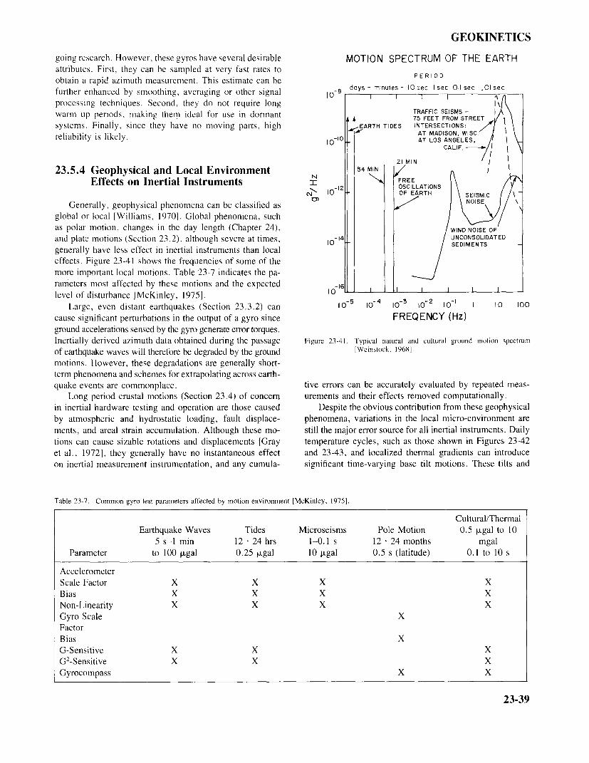
GEOKINETICS

going research. However, these gyros have several desirable MOTION SPECTRUM OF THE EARTHattributes. First, they can be sampled at very fast rates toobtain a rapid azimuth measurement. This estimate can be PERIODfurther enhanced by smoothing, averaging or other signalprocessing techniques. Second, they do not require longwarm up periods, making them ideal for use in dormant TRAFFIC SEISMS -

75 FEET FROM STREET

systems. Finally, since they have no moving parts, high EARTH TIDES INTERSECTIONS:reliability is likely. AT MADISON, WISC.

AT LOS ANGELES,CALIF.

23.5.4 Geophysical and Local EnvironmentEffects on Inertial Instruments FREE

OSCILLATIONSOF EARTH SEISMIC

Generally, geophysical phenomena can be classified as NOISE

global or local [Williams, 1970]. Global phenomena, suchas polar motion, changes in the day length (Chapter 24), WIND NOISE OF

and plate motions (Section 23.2), although severe at times, UNCONSOLIDATED

generally have less effect in inertial instruments than localeffects. Figure 23-41 shows the frequencies of some of themore important local motions. Table 23-7 indicates the pa-rameters most affected by these motions and the expectedlevel of disturbance [McKinley, 1975].

Large, even distant earthquakes (Section 23.3.2) cancause significant perturbations in the output of a gyro since FREQENCY (Hz)ground accelerations sensed by the gyro generate error torques.Inertially derived azimuth data obtained during the passage Figure 23-41. Typical natural and cultural ground motion spectrum

of earthquake waves will therefore be degraded by the ground [Weinstock, 1968].motions. However, these degradations are generally short-term phenomena and schemes for extrapolating across earth-quake events are commonplace. tive errors can be accurately evaluated by repeated meas-

Long period crustal motions (Section 23.4) of concern urements and their effects removed computationally.in inertial hardware testing and operation are those caused Despite the obvious contribution from these geophysicalby atmospheric and hydrostatic loading, fault displace- phenomena, variations in the local micro-environment arements, and areal strain accumulation. Although these mo- still the major error source for all inertial instruments. Dailytions can cause sizable rotations and displacements [Gray temperature cycles, such as those shown in Figures 23-42et al., 1972], they generally have no instantaneous effect and 23-43, and localized thermal gradients can introduceon inertial measurement instrumentation, and any cumula- significant time-varying base tilt motions. These tilts and

Table 23-7. Common gyro test parameters affected by motion environment [McKinley, 19751.

Cultural/ThermalEarthquake Waves Tides Microseisms Pole Motion 0.5 ugal to 10

5 s-l min 12 24 hrs 1-0.1 s 12 24 months mgalParameter to 100 ugal 0.25 ugal 10 ugal 0.5 s (latitude) 0.1 to 10 s

AccelerometerScale Factor X X X XBias X X X XNon-Linearity X X X XGyro Scale XFactorBias XG-Sensitive X X XG2-Sensitive X X XGyrocompass X X

23-39

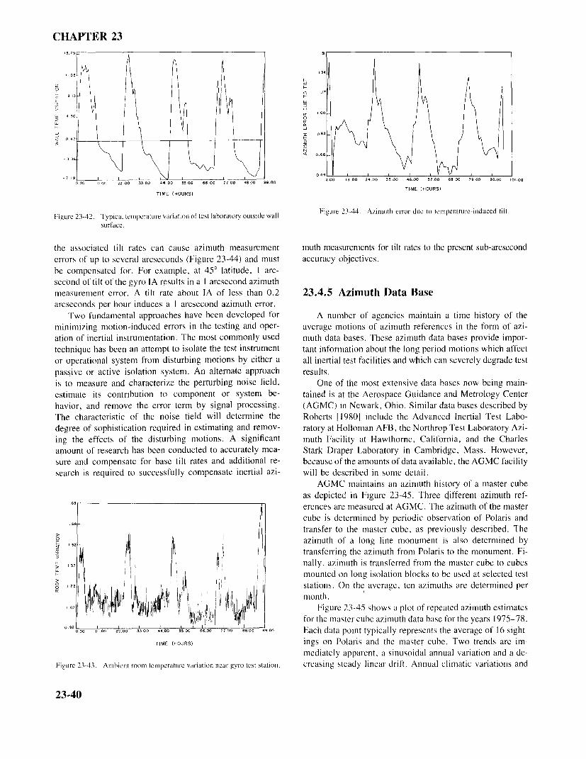
CHAPTER 23

0

0

TIME (HOURS)TIME (HOURS)

Figure 23-44. Azimuth error due to temperature-induced tilt.Figure 23-42. Typical temperature variation of test laboratory outside wall Figure 23-44. Azimuth error due to temperature-indced tilt.

surface.

the associated tilt rates can cause azimuth measurement muth measurements for tilt rates to the present sub-arcseconderrors of up to several arcseconds (Figure 23-44) and must accuracy objectives.be compensated for. For example, at 45o latitude, I arc-second of tilt of the gyro IA results in a I arcsecond azimuthmeasurement error. A tilt rate about IA of less than 0.2 23.4.5 Azimuth Data Basearcseconds per hour induces a 1 arcsecond azimuth error.

Two fundamental approaches have been developed for A number of agencies maintain a time history of theminimizing motion-induced errors in the testing and oper- average motions of azimuth references in the form of azi-ation of inertial instrumentation. The most commonly used muth data bases. These azimuth data bases provide impor-technique has been an attempt to isolate the test instrument tant information about the long period motions which affector operational system from disturbing motions by either a all inertial test facilities and which can severely degrade testpassive or active isolation system. An alternate approach results.is to measure and characterize the perturbing noise field, One of the most extensive data bases now being main-estimate its contribution to component or system be- tained is at the Aerospace Guidance and Metrology Centerhavior, and remove the error term by signal processing. (AGMC) in Newark, Ohio. Similar data bases described byThe characteristic of the noise field will determine the Roberts [1980] include the Advanced Inertial Test Labo-degree of sophistication required in estimating and remov- ratory at Holloman AFB, the Northrop Test Laboratory Azi-ing the effects of the disturbing motions. A significant muth Facility at Hawthorne, California, and the Charlesamount of research has been conducted to accurately mea- Stark Draper Laboratory in Cambridge, Mass. However,sure and compensate for base tilt rates and additional re- because of the amounts of data available, the AGMC facilitysearch is required to successfully compensate inertial azi- will be described in some detail.

AGMC maintains an azimuth history of a master cubeas depicted in Figure 23-45. Three different azimuth ref-erences are measured at AGMC. The azimuth of the mastercube is determined by periodic observation of Polaris andtransfer to the master cube, as previously described. Theazimuth of a long line monument is also determined bytransferring the azimuth from Polaris to the monument. Fi-nally, azimuth is transferred from the master cube to cubesmounted on long isolation blocks to be used at selected teststations. On the average, ten azimuths are determined per

Figure 23-45 shows a plot of repeated azimuth estimatesmonth.for the master cube azimuth data base for the years 1975-78.

Each data point typically represents the average of 16 sight-TIME (HOURS) ings on Polaris and the master cube. Two trends are im-

mediately apparent, a sinusoidal annual variation and a de-Figure 23-43. Ambient room temperature variation near gyro test station. creasing steady linear drift. Annual climatic variations and

23-40

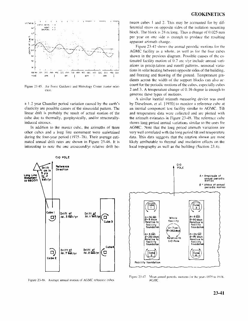
GEOKINETICS

tween cubes I and 2. This may be accounted for by dif-GRAND MEAN = 1 3

58. RAMP 13 ferential stress on opposite sides of the isolation mountingSINUSOID =12

57" block. The block is 24 m long. Thus a change of 0.025 mmper year on one side is enough to produce the resultingapparent azimuth change.

Figure 23-47 shows the annual periodic motions for the54" AGMC facility as a whole, as well as for the four cubes

53" shown in the previous diagram. Possible causes of the es-52" timated facility motion of 0.7 arc s/yr include annual vari-

ations in precipitation and runoff patterns, seasonal varia-tions in solar heating between opposite sides of the building,

DAY NO 100 200 300 400 500 600 700 800 900 1000 1100 1200 1300 1400 1500

YEAR 1975 1976 1977 1978 and freezing and thawing of the ground. Temperature gra-dients across the width of the support blocks can also ac-

Figure 23-45. Air Force Guidance and Metrology Center master refer- count for the periodic motions of the cubes, especially cubesencc. 2 and 3. A temperature change of O. 16 degree is enough to

generate these types of motions.A similar inertial azimuth measuring device was used

a 1.2 year Chandler period variation caused by the earth's by Dieselman, et al. 119701 to monitor a reference cube atelasticity are possible causes of the sinusoidal pattern. The an inertial component test facility similar to AGMC. Tiltlinear drift is probably the result of actual motion of the and temperature data were collected and are plotted withcube due to thermally, geophysically, and/or structurally- the azimuth estimates in Figure 23-48. The reference cubeinduced stresses. shows long period annual variations similar to the ones for

In addition to the master cube, the azimuths of three AGMC. Note that the long period azimuth variations areother cubes and a long line monument were maintained very well correlated with the long period tilt and temperatureduring the four-year period (1975-78). Their average esti- data. This data suggests that the rotation shown are mostmated annual drift rates are shown in Figure 23-46. It is likely attributable to thermal and insolation effects on theinteresting to note the one arcsecond/yr relative drift be- local topography as well as the building (Section 23.4).

CIO POLE

CIOReference POLEDirection

Long Line A = Amplitude ofMonument annual periodic= 6600ft motion

8 = phase of annualperiodic motion

Cube I Drift of Dritt, ofWhole A=.6 sec

Cube 3 Relative to facility Relative to

foundation A =.7 sec foundationB = 362days

A=.6 sec A=.05 sec

B=261 days Relative to B=181 days

facility CIO Pole facility

Cube4Drift of Drift of=. 7 sec/yr =.2 sec/yr

Cube 2Facility foundation

Figure 23-47. Mean annual periodic motions for the years 1975 to 1978.Figure 23-46. Average annual motion of AGMC reference cubes. AGMC.

23-41

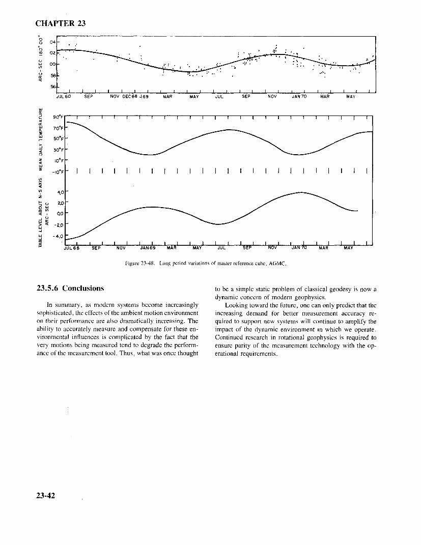
CHAPTER 23

0

58

56

JUL 60 SEP NOV DEC68 J.69 MAR MAY JUL SEP NOV JAN70 MAR MAY

70oF

50oF

30oF

1O°F

-4.0

-4.0

JUL68 SEP NOV JAN69 MAR MAY JUL SEP NOV JAN70 MAR MAY

Figure 23-48. Long period variations of master reference cube, AGMC.

23.5.6 Conclusions to be a simple static problem of classical geodesy is now adynamic concern of modern geophysics.

In summary, as modern systems become increasingly Looking toward the future, one can only predict that thesophisticated, the effects of the ambient motion environment increasing demand for better measurement accuracy re-on their performance are also dramatically increasing. The quired to support new systems will continue to amplify theability to accurately measure and compensate for these en- impact of the dynamic environment in which we operate.vironmental influences is complicated by the fact that the Continued research in rotational geophysics is required tovery motions being measured tend to degrade the perform- ensure parity of the measurement technology with the op-ance of the measurement tool. Thus, what was once thought erational requirements.

23-42

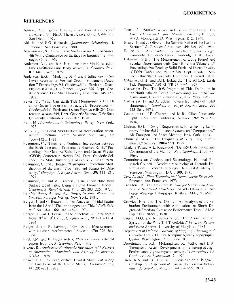
GEOKINETICS

REFERENCES

Agnew, D.C., Strain Tides at Pinon Flat: Analysis and Brune, J., "Surface Waves and Crustal Structures." TheInterpretation, Ph.D. Thesis, University of California, Earth's Crust and Upper Mantle, edited by P. Hart.San Diego, 1979. AGU, Monograph 13, Washington, D.C. 1969.

Aki, K. and P.G. Richards, Quantitative Seismology, 1, Brune, J. and J. Oliver. "The Seismic Noise of the Earth'sFreeman, San Francisco, 1980. Surface," Bull. Seismol. Soc. Am., 49: 349-353, 1959.

Algermissen, S., Seismic Risk Studies in the United States, Bullen, K.E., An Introduction to the Theory of Seisiology,4th World Conference on Earthquake Engineering, San- Cambridge University Press, Cambridge, U.K., 1965.tiago, Chile, 1969. Cabaniss, G.H., "The Measurement of Long Period and

Anderson, D.L. and R.S. Hart, "An Earth Model Based on Secular Deformation with Deep Borehole Tiltmeters,"Free Oscillations and Body Waves," J. Geophys. Res., Proceedings 9th Geodesy/Solid Earth and Ocean Physics81: 1461-1475, 1976. (GEOP) Conference, Report 280, Dept. Geodetic Sci-

Anderson, E.G., "Modeling of Physical Influences in Sea ence, Ohio State University, Columbus, 165-169, 1978.Level Records for Vertical Crustal Movement Detec- Cabaniss, G.H. and D.H. Eckhardt, "The AFCRL Earthtion," Proceedings 9th Geodesy/Solid Earth and Ocean Tide Program," AFCRL TR-73-0084, 1973.Physics (GEOP) Conference, Report 280, Dept. Geo- Cartwright, D., "The IOS Program of Tidal Definition indetic Science, Ohio State University, Columbus, 145 152, the North Atlantic Ocean." Proceedings 9th Earth Tide1978. Symposium, Columbia University, New York, 1982.

Baker, T., "What Can Earth Tide Measurements Tell Us Cartwright, D. and A. Edden, "Corrected Tables of Tidalabout Ocean Tide or Earth Structure'?," Proceedings 9th Harmonics," Geophys. J. Royal Astron. Soc., 33:Geodesy/Solid Earth and Ocean Physics (GEOP) Con- 253-264, 1973.ference, Report280, Dept. Geodetic Science, Ohio State Castle, R.O., J.P. Church, and M.R. Elliot, "AseismicUniversity, Columbus, 299-307, 1978. Uplift in Southern California," Science, 192: 251 253,

Bath, M., Introduction to Seismology, Wiley, New York, 1976.1973. Chilton, E.G., "Design Requirements for a Testing Labo-

Battis, J., "Regional Modification of Acceleration Atten- ratory for Inertial Guidance Systems and Components,"uation Functions," Bull. Seismol. Soc. Am., 71: Air Transport and Space Meeting, New York, 1964.1309-1321, 1981. Chinnery, M.A., "The Frequency of Very Large Earth-

Beaumont, C., "Linear and Nonlinear Interactions between quakes," Science, 190(4222), 1975.the Earth Tide and a Tectonically Stressed Earth," Pro- Clark, S.P. and A.E. Ringwood, "Density Distribution andceedings 9th Geodesy/Solid Earth and Ocean Physics Constitution of the Mantle," Rev. Geophys., 2: 35-88,(GEOP) Conference, Report 280, Dept. Geodetic Sci- 1964.ence, Ohio State University, Columbus, 313-318, 1978. Committees on Geodesy and Seismology, National Re-

Beaumont, C. and J. Berger, "Earthquake Prediction: Mod- search Council, "Geodetic Monitoring of Tectonic De-ification of the Earth Tide Tilts and Strains by Dila- formation - Toward a Strategy," National Academy oftancy," Geophys. J. Royal Astron. Soc., 39: 111-121, Sciences, Washington. D.C., 109, 1981.1974. Cox, A. (ed.), Plate Tectonics and Geomagnetic Reversals,

Beaumont, C. and A. Lambert, "Crustal Structure from Freeman, San Francisco, 1973.Surface Load Tilts, Using a Finite Element Model," Crowford, R., The Air Force Manual for Design and Anal-Geophys. J. Royal Astron. Sec., 29: 203 226, 1972. ysis of Hardened Structures, AFWL-TR-74-102, Air

Ben-Menahem, A. and S.J. Singh, Seismic Waves and Force Weapons Laboratory, Kirtland AFB, N. Mex.,Sources, Springer Verlag, New York, 1981. 1974.

Berger, J. and C. Beaumont, "An Analysis of Tidal Strains Crowley, F.A. and H.A. Ossing, "An Analysis of the Vi-from the USA: II The Inhomogeneous Tide." Bull. Seis- bration Environment with Applications to Single-De-mol. Soc. Am., 66: 1821-1846, 1976. gree-of-Freedom Gyroscope Performance Tests," AIAA

Berger, J. and J. Levine, "The Spectrum of Earth Strain Paper No. 70-951, 1970.from 10-8 to 102 Hz,"J. Geophys. Res., 79: 1210-1214, Currie, D.G. and R. Salvermoser, "The Array Eyepiece1974. System for the Wild T-4 Theodolite," Program Review

Berger, J. and R. Lovberg, "Earth Strain Measurements and Field Results, University of Maryland, 1981.with a Laser Interferometer," Science, 170: 296-303, Department of Defense, Glossary of Mapping, Charting and1970. Geodetic Terins, Defense Mapping Agency Topographic

Bird, J.M. and B. Isacks (eds.), Plate Tectonics, selected Center, Washington, D.C., June 1973.papers from the J. Geophys. Res., 1972. Dieselman, J., R.L. McLaughlin, K. Millo, and L.B.

Brazee, R., Analysis of Earthquake Intensities With Respect Thompson, "Recent Developments in the Testing of Highto Attenuation, Magnitude and Rate of Recurrence, Performance Gyrocompass Devices," Proceedings 5thNOAA, 1976. Guidance Test Symposium, 2, 1970.

Brown, L.D., "Recent Vertical Crustal Movement Along Dietz, R.S. and J.C. Holden, "Reconstruction to Pangaea:the East Coast of the United States," Tectonophysics, Breakup and Dispersion of Continents, Permian to Pre-44: 205-231, 1978. sent,"J. Geophys. Res.. 75: 4939-49-56, 1970.

23-43

CHAPTER 23

Donovan, N., B. Bolt, and R. Whitman. Technology Re- Jaenke, M.G., "A Proposed Model for the Rotational Mo-view, Cambridge. Mass.. May 1977. tions of a Test Pad," AIAA Paper No. 74-855, 1974.

Dorman, J., "Seismic Surface Wave Data on the Upper Johnston, J.C., Z.A. Cybriwsky, and G.K. Leblanc, "TheMantle," The Earth's Crust and Upper Mantle, edited Regulatory Guide 1.60 Its Content and Applicability"by P.J. Hart, AGU, Monograph 13, Washington, D.C., abstract, Earthquake Notes, 51(3), 1980.1969. Kanamori, H.. "Velocity and Q of Mantle Waves," Phys.

Everndon, J.F.. "Gravity Profiles in Southern California," Earth Planet. Int., 2: 259-275, 1970.Earthquake Prediction: An International Review, AGU, Kanamori, H. and J. Cipar, "Focal Process of Great ChileanWashington, D.C. 485-496, 1981. Earthquake," May 22, 1960, Phys. Earth Planet. Int.,

Ewing, C.E. and M.M. Mitchell, Introduction to Geodesy, 9: 128-136, 1974.Elsevier, New York, 1970. Kanamori, H., "The Energy Release in Great Earthquakes,"

Farrell, W.E., "Deformation of the Earth by Surface Loads," J. Geophys. Res., 82(20), 1977.Rev. Geophvs. Space Phys., 10: 761-797, 1972. Kayton, M., "Fundamental Limitations on Inertial Mea-

Fix, J., "Ambient Earth Motions in the Period Range from surements," Guidance and Control, Academic Press,0.1 to 2560 Sec, Bull. Seismol. Soc. Am., 62: 1753-1760, New York, 1962.1972. Kuo, J.T., "Static Response of a Multilayered Medium Un-

Garland, G.D., Introduction to Geophysics, W.B. Saunders der Inclined Surface Loads," J. Geophys. Res., 74:Co., Philadelphia, 1971. 3195 3207, 1969.

Gass, I.G., "Ophiolites," Sci. Am., August 1982. Kuo, J.T., "The Inverse Problem: Ocean Tides DerivedGoad, C.C., "Gravimetric Tidal Loading Computed from from Earth Tide Observations," Proceedings 9th Geo-

Integrated Green's Functions," J. Geophys. Res., 85: desy/Solid Earth and Ocean Physics (GEOP) Confer-2679-2683, 1980. ence, Report 280, Dept. Geodetic Science, Ohio State

Gray, R.A., G.H. Cabaniss, F.A. Crowley, H.A. Ossing, University, Columbus, 319 326, 1978.T.S. Rhoades, and L.B. Thompson, "Earth Motions and Lambert, A. and C. Beaumont, "Nano Variations in GravityTheir Effects on Inertial Instrument Performance," Due to Seasonal Groundwater Movements: ImplicationsAFCRL-72-0278, AD748274, 1972. for the Gravitational Detection of Tectonic Movements,"

Greensfelder, R., "Maximum Credible Rock Acceleration J. Geophys. Res., 82, 297-306, 1977.from Earthquakes in California," California Division of Lambert, A. and J.O. Liard, "A Search for Long-TermMines and Geology, Map Sheet 25, 1974. Earthquake Precursors in Gravity Data in the Charle-

Harrison, J.C., "Cavity and Topographic Effects in Tilt and voix Region, Quebec," Earthquake Prediction: An In-Strain Measurement," J. Geophys. Res., 81: 319 328, ternationalReview, AGU, Washington, D.C.,473-483,1976. 1981.

Harrison, J.C., "Implications of Cavity, Topographic, and Lennon, G.W. and T.F. Baker, "The Earth Tide Signal andGeologic Influences on Tilt and Strain Measurements," Its Coherency," Qtrly. J. Roy. Astron. Soc., 14: 161-182,Proceedings 9th Geodesy/Solid Earth and Ocean Phy- 1973.sics (GEOP) Conference, Report 280, Dept. Geodetic Levine, J., "Strain-Tide Spectroscopy," Geophys. J. RoyalScience, Ohio State University, Columbus, 283-287, Astron. Soc., 54: 27-41, 1978.1978. Levine, S.A. and A. Gelb, "Geodetic and Geophysical Un-

Harrison, J.C., and K. Herbst, "Thermoelastic Strains certainties Fundamental Limitations on Terrestrial In-and Tilt Revisted," Geophys. Res. Lett., 4: 535-537, ertial Navigation," AIAA Guidance Control and Flight1977. Dynamics Conference, Pasadena, Calif., 1968.

Herbst, K., "Interpretation of Tilt Measurements in the Pe- Lewkowicz, J.F. and G.H. Cabaniss, "Near-Field Staticriod Range above that of the Tides," AFGL-TR-79- Tilts from Surface Loads," AFGL-TR-80-0221,0093, ADA074525 (Translation No. 109), 1979. ADA094123, 1980.

Holzner, T.L., S.N. Davis, and B.E. Lofgren, "Faulting Lindh, A.G. and D.M. Boore, "Control of Rupture by FaultCaused by Groundwater Extraction in South-Central Ar- Geometry During the 1966 Parkfield Earthquake," Bull.izona," J. Geophys. Res., 84: 603-612, 1979. Seismo. Soc. Am., 71, 95-116, 1981.

Huggett, G.R., L.E. Slater, and J. Langbein, "Fault Slip Longman, I.M., "A Green's Function for Determining theEpisodes near Hollister, California: Initial Results Using Deformation of the Earth Under Surface Mass Loads,a Multiwavelength Distance Measuring Instrument," J. I. Theory," J. Geophys. Res., 67: 845-850, 1962.Geophys. Res., 82: 3361-3368, 1977. McGuire, R., FORTRAN Computer Program for Seismic

Isacks, B., J. Oliver, and L. Sykes, "Seismology and Risk Analysis, U.S. Geological Survey, Open File Re-the New Global Tectonics," J. Geophys. Res., 73:(18), port, 76-67, 1976.1968. McKinley, H.L.. "Geokinetic and Geophysical Influence

Iyer, H., The History of Science of Microseisms, VESIAC on 1980's ICBM Guidance," AIAA Guidance and Con-Report 4410-64-X, University of Michigan, Ann Arbor, trol Conference, Boston, Mass, 1975.1964. Melchior, P., The Earth Tides, Pergamon Press, Oxford,

Jackson, D.D. and W.B. Lee, "The Palmdale Bulge An 1966.Alternate Interpretation," Eos, Trans. AGU, 60, 810, Minster, J.B. and T.H. Jordan, "Present day plate motions,"1979. J. Geophys. Res., 83: 5331 5354, 1978.

23-44

GEOKINETICS

Mogi, K., "Earthquake Prediction in Japan," Earthquake Shearer, J.A., "Error Analysis and Performance Data fromPrediction: An International Review, AGU, Washing- an Automated Azimuth Measuring System," AIAA Pa-ton, D.C., 635-666, 1981. per No. 80-1793, 1980.

Morgan, W.J., "Rises, Trenches, Great Faults, and Crustal Simmons, B.J., R.M. Hanes, and F.S. Heming, "DynamicBlocks," J. Geophys. Res., 73: 1959, 1968. Analysis of Test Platform," AIAA Paper No. 81-1816,

Morgan, W.J., "Plate Motions and Deep Mantle Convec- 1981.tion," Studies in Earth and Space Sciences, Geol. Soc. Simpson, D.W. and P.G. Richards (eds.), Earthquake Pre-Amer. Mem. 132, 1972. diction: An International Review, AGU, Washington,

Mueller, Ivan I., Spherical and Practical Astronomy as D.C., 1981.Applied to Geodesy, Ungar, New York, 1969. Slemmons, D., Faults and Earthquake Magnitude, U.S.

Nuttli, O., "The Mississippi Valley Earthquakes of 1811 Army Engineers Waterways Experimentation Station,and 1812: Intensities, Ground Motion and Magnitudes," Miscellaneous Paper S-73-1, 1977.Bull. Seismol. Soc. Am., 63: 227-248, 1973. Smith, D.E., "Spaceborn Ranging System," Proceedings

Nuttli, O., The Relation of Sustained Maximum Ground 9th Geodesy/Solid Earth and Ocean Physics (GEOP)Acceleration and Velocity to Earthquake Intensity and Conference, Report 280, Dept. Geodetic Science, OhioMagnitude, U.S. Army Engineer Waterways Experi- State University, Columbus, 59-64, 1978.mentation Station, Miscellaneous Paper S-73-1, 1979. Smith, D.E., R. Kolenkiewicz, P.J. Dunn, and M.H.

Ossing H. and R. Gray, A Survey of the Ambient Motion Torrence, "The Measurement of Fault Motion by Sat-Environment in the Southwestern United States, In- ellite Laser Ranging," Tectonophysics, 52: 59-67,terim Scientific Report AFGL-TR-78-0052, ADA056872, 1979.1978. Stein, R.S., "Discrimination of Tectonic Displacement from

Parke, M.E., "Open Ocean Tide Modelling," Proceedings Slope Dependent Errors in Geodetic Leveling from9th Geodesy/Solid Earth and Ocean Physics (GEOP) Southern California, 1953-1979," Earthquake Predic-Conference, Report 280, Dept. Geodetic Science, Ohio tion: An International Review, AGU, Washington, D.C.,State University, Columbus, 289-297, 1978. 441-456, 1981.

Predicting Earthquakes, Panel on Earthquake Prediction, Strange, W., "The Impact of Refraction Correction on Lev-National Academy of Sciences, Washington, D.C., 1976. eling Interpretations in Southern California," J. Geo-

Raisler, R.B. and J.C. Fatz, "Stability of Stable Areas," phys. Res., 86: 2809-2824, 1981.AIAA Paper No. 74-859, 1974. Takeuchi, H., "On the Earth Tide," J. Fac. Sci, University

Reilinger, R. and L.D. Brown, "Neotectonic deforma- of Tokyo, Sec 11-7; Part II, 1-7, 1951.tion, near surface movements and systematic errors in Tsutsumi, K., "A Program of Study on Long-Term EarthU.S. releveling measurements: Implications for earth- Tilts," AFCRL-70-0268, AD724868, 1970.quake prediction," Earthquake Prediction: An Inter- Verhoogen, J., F.J. Turner, L.E. Weiss, C. Wahrhaftig,national Review, AGU, Washington, D.C., 422-440, and W.S. Fyfe, The Earth: An Introduction to Physical1981. Geology, Holt, Rinehart & Winston, New York, 1970.

Richter, C., Elementary Seismology, Freeman, San Fran- Wahr, J.M., The Tidal motions of a Rotating, Elliptical,cisco, 1958. Elastic, and Oceanless Earth, Ph.D Thesis, University

Roberts, G.E., "MX laboratory azimuth data base study of Colorado, 1979.(Status report)," Geodynamics Corporation, Santa Bar- Walcott, R.I., "Late Quaternary Vertical Movements inbara, CDR-0008 (SR38OU)-1, 1980. Eastern North America: Quantitative Evidence of Gla-

Savage, J.C., W.H. Prescott, M. Lisowski, and N.E. King, cio-Isostatic Rebound," Rev. Geophys. Space Phys., 10:"Strain Accumulation in Southern California 1973-1980," 849-884, 1972.J. Geophys. Res., 86: 6991-7001, 1981. Weinstock, H., "Design of Precision Tilt and Rotational

Schureman, P., "Manual of Harmonic Analysis and Pre- Vibration Isolation System for Inertial Sensor Testing,"diction of Tides," Spec. Pub. 98, U.S. Coast and Geo- AIAA Paper No. 68-894, 1968.detic Survey, 1958. Whitcomb, J.H., "New Vertical Geodesy," J. Geophys.

Schwiderski, E.W., "Ocean tides, Part I: Global Tidal Equa- Res., 81: 4937-4944, 1976.tions," Marine Geodesy, 3: 161-187, 1979. Williams, O.W., "A Review of Geophysical Effects and

Schwiderski, E.W., "On Charting Global Ocean Tides," Suggested Testing Conditions Related to Advanced In-Rev. Geophys. Space Phys., 18: 38-61, 1980. ertial Components" Paper presented to USAF Scientific

Schwiderski, E.W., "Ocean tides, Part 11: A Hydro- Advisory Board Ad Hoc Committee on Geophysicaldynamic Interpolation Model,"Marine Geodesy, 3:219- Effects on Inertial Instruments, 1970.255, 1980. Willmore, P. L. (ed.), Manual of Seismological Observatory

Seismic Noise Survey, Geotech Technical Report 63-45, 1: Practice, World Data Center A for Solid Earth Geo-Garland Texas, 1963. physics, Report SE-20, 1979.

Seismic Noise Survey, Geotech Technical Report 63-45, 2: Wilson, J.T., "A New Class of Faults and their Bearing onGarland, Texas, 1963. Continental Drift," Nature 207: 343-347, 1965.

Shearer, J.A., "Evaluation of an Advanced Gyro and Wheel Wittry, J.R., "Description of an Inertial Test Facility In-Speed Modulation for Highly Accurate Azimuth Deter- corporating a Passively Isolated and Actively Stabilizedmination," AFGL-TR-82-0016, AD114640, 1982. Platform," AIAA Paper No. 69-863, 1969.

23-45

CHAPTER 23

Wyatt, F., "Displacement of Surface Monuments: Hor- Zienkiewicz, O.C., The Finite Element Method in Struc-izontal Motion," J. Geophys. Res., 87: 979-989, tural and Continuum Mechanics, McGraw-Hill, New1982. York, 1967.

Wyatt, F., G.H. Cabaniss, and D.C. Agnew, "A Compar- Zschau, J., "Tidal Sea Load Tilt of the Crust, and Its Ap-ison of Tiltmeters at Tidal Frequencies," Geophys. Res. plication to the Study of Crustal and Upper Mantle Struc-Ltrs., 9: 743-746, 1982. ture," Geophys. J. Royal Astron. Soc., 44: 577-593,

Wyllie, P.J., The Dynamic Earth, Wiley, New York, 1971. 1976.

23-46