Fè et al. BMC Genomics (2015) 16:921 DOI 10.1186/s12864-015-2163-3

RESEARCH ARTICLE Open Access

Genomic dissection and prediction ofheading date in perennial ryegrass

Dario Fè1,3*, Fabio Cericola1, Stephen Byrne2, Ingo Lenk3, Bilal Hassan Ashraf1, Morten Greve Pedersen3,Niels Roulund3, Torben Asp2, Luc Janss1, Christian Sig Jensen3 and Just Jensen1

Abstract

Background: Genomic selection (GS) has become a commonly used technology in animal breeding. In crops, it isexpected to significantly improve the genetic gains per unit of time. So far, its implementation in plant breedinghas been mainly investigated in species farmed as homogeneous varieties. Concerning crops farmed in familypools, only a few theoretical studies are currently available. Here, we test the opportunity to implement GS inbreeding of perennial ryegrass, using real data from a forage breeding program. Heading date was chosen as amodel trait, due to its high heritability and ease of assessment. Genome Wide Association analysis was performedto uncover the genetic architecture of the trait. Then, Genomic Prediction (GP) models were tested and predictionaccuracy was compared to the one obtained in traditional Marker Assisted Selection (MAS) methods.

Results: Several markers were significantly associated with heading date, some locating within or proximal togenes with a well-established role in floral regulation. GP models gave very high accuracies, which weresignificantly better than those obtained through traditional MAS. Accuracies were higher when predictions weremade from related families and from larger training populations, whereas predicting from unrelated families causedthe variance of the estimated breeding values to be biased downwards.

Conclusions: We have demonstrated that there are good perspectives for GS implementation in perennial ryegrassbreeding, and that problems resulting from low linkage disequilibrium (LD) can be reduced by the presence ofstructure and related families in the breeding population. While comprehensive Genome Wide Association analysisis difficult in species with extremely low LD, we did identify variants proximal to genes with a known role inflowering time (e.g. CONSTANS and Phytochrome C).

Keywords: Genomic selection, Perennial ryegrass, Heading, Flowering, GWAS, Lolium, CONSTANS, Phytochrome,Accuracy

BackgroundPerennial ryegrass (Lolium perenne L.) is one of the mostcultivated forage species in temperate grasslands, mainlyfarmed for its re-growth capacity after defoliation, andfor the high value as feed for ruminants, due to palat-ability, digestibility, and nutritive contents [1–3]. Peren-nial ryegrass is an obligate allogamous species withgenetic gametophytic self-incompatibility [4], and is bredin genetically heterogeneous families.

* Correspondence: dfe@dlf.com1Department of Molecular Biology and Genetics, Center for QuantitativeGenetics and Genomics, Aarhus University, Blichers Allé 20, 8830 Tjele,Denmark3DLF A/S, Research Division, Højerupvej 31, 4660 Store Heddinge, DenmarkFull list of author information is available at the end of the article

© 2015 Fè et al. Open Access This article is dLicense (http://creativecommons.org/licenses/medium, provided you give appropriate crediCommons license, and indicate if changes wecreativecommons.org/publicdomain/zero/1.0/

Heading date (HD) is an important trait for foragespecies, often used as a model trait [5, 6] due to its highheritability and the ease of assess. It follows the shiftfrom vegetative to reproductive growth, and it is signifi-cantly correlated with several other traits involved inplant growth and development, such as plant height,spike length, tiller number and size, leaf length [7, 8], aswell as with a number of yield and quality traits. Earlyheading genotypes show a higher growth rate in springand higher forage yield in the first cut, [9–12]. Corres-pondingly, the opposite was found for later cuts in sum-mer, where dry matter forage yield was higher for lategenotypes. Results in the literature are inconsistent re-garding performances in fall and winter. Humphreys [9]found higher autumn and winter growth rate in late

istributed under the terms of the Creative Commons Attribution 4.0 Internationalby/4.0/), which permits unrestricted use, distribution, and reproduction in anyt to the original author(s) and the source, provide a link to the Creativere made. The Creative Commons Public Domain Dedication waiver (http://) applies to the data made available in this article, unless otherwise stated.

Fè et al. BMC Genomics (2015) 16:921 Page 2 of 15

genotypes, while in Sampoux et al. [11], the correlationbetween HD and forage yield in autumn was not signifi-cantly different from zero. Differences between early andlate genotypes were also observed in the intensity ofaftermath heading, which was higher in the early mater-ial [9, 11, 12], as well as in the content of fiber and sol-uble sugars. Humphreys [9] and Sampoux et al. [11]measured less water soluble carbohydrates and more lig-nin and neutral detergent fiber in early- than in late HDvarieties. Late heading was also associated with higherdigestibility and therefore to a higher lactation energycontent for milk production [10]. Although heading alsomarks the production of seeds, the correlation with seedyield is unclear. Later genotypes were generally found togive lower seed production [13, 14], but this correlationwas not always significant [8, 14].Due to its significant effects on other traits, breeding

has always aimed to exploit the natural variation in HD,in order to create mixtures of varieties that could givehigh performances throughout the whole year. SinceInternational listing of new varieties requires fulfilmentof the three criteria; distinctiveness, uniformity, and sta-bility (DUS) there is also a strong breeding focus on HDin order to create uniform varieties. While the uniform-ity of inbred varieties is rather easy to control it can bemore challenging in outbreeding grass varieties that arebreed as families.In order to ensure more stability in forage quality

over the season, cultivars have been divided into dif-ferent earliness groups. The number- and extend ofeach HD group differs between countries, with somecountries defining up to nine HD groups. However,HD appears to behave as a continuous character, andthe distinction between early and late material is notalways clear, with new candidates that may be classi-fied in different neighboring HD groups, dependingon the definitions used in the different countries.The trait always showed medium to high heritability[9, 12, 14–16]. Kearsey et al. [15] showed the pres-ence of both additive and dominance effects, withthe first being the larger and dominance being forearly heading, but did not find any evidence forepistasis. Genotype by environment (G × E) interac-tions were found to be small by Ravel and Charmet[16], in a multi-site analysis in France. However, adifferent result was obtained by Kearsey et al. [15],who showed interactions between the environment andboth additive and dominance effects, in an experimentacross Italy and the UK.In the latter decade, the genetic control of HD was

better understood thanks to the use of molecularmarkers and comparative genome analyzes. In modelspecies, such as Arabidopsis thaliana L., as well as in ce-reals like wheat and rice heading or the control of

flowering has been the subject for numerous studies andpublications (reviewed in [17–19]). Especially the use ofinduced Arabidopsis mutants and the combinations ofsuch lead to the detailed modelling of the genetic con-trol of flowering in plants. The investigations demon-strated the involvement of genes belonging to threemajor pathways: (i) vernalization response genes (Vrn),which regulates heading after low temperature periods;(ii) photoperiod response genes (Ppd), which is active/in-active with a certain day length; (iii) ‘earliness per se’ fac-tors, which seems to be independent of light and coldrequirements [20].In perennial ryegrass a number of flowering genes

were previously identified by sequence homology withflowering genes found in Arabidopsis, rice, and maize[17, 21–23]. Others were identified through classicalQuantitative Trait Loci (QTL) mapping, performed usingdifferent plant material and different genetic maps. Gen-etic maps were organized in seven linkage groups (LGs),numbered according to the conserved synteny with theTriticeae’s maps [24]. QTLs were identified on all sevenLGs [7, 8, 25–29]. Comparison between studies is com-plicated due to lack of common markers and it is alwaysdifficult to determine if two significant markers foundon the same LG, actually correspond to the same QTL.Furthermore, among different studies there is often pooragreement regarding the number and the distribution ofthe QTLs, likely due to environmental factors, use of dif-ferent mapping populations [30], and low statisticalpower in several studies. A great effort was put in under-standing the genetic mechanisms behind the QTLs inLG4 and LG7, which were significant in almost all stud-ies. The first was found to be in a syntenic associationwith the wheat Vrn1 gene [26], and its function seems tobe conserved between diploid wheat and perennial rye-grass [19]. A relation was also hypothesized with a puta-tive casein kinase gene, previously mapped in rice andinvolved in photoperiod sensitivity [29]. The QTL onLG7 was suggested to be associated with the gene LpCO,homologous to the CONSTANS of Arabidopsis and theHd1 of rice, involved in the photoperiodic regulation offlowering time [17, 31, 32]. Synteny was also detectedwith the Hd3 region of rice [25], which codes for aFLOWERING-LOCUS-T (FT) orthologue of Arabidopsis.FT gene is involved in induction to reproductive growthat the meristem [33, 34] and has been shown to activelyregulate the flowering response in L. perenne [35]. Otherhypothesis have been proposed to relate the other sig-nificant markers to QTL previously found in related spe-cies, such as Lolium multiforum Lam. and Festucapratensis L. [29].While these studies identified some of the key genes in

floral control in ryegrass, the biology of the trait is stillfar from being understood. Furthermore, the use of QTL

Fè et al. BMC Genomics (2015) 16:921 Page 3 of 15

analyses was shown to be not effective in capturing smalleffect genes [36] and to overestimate the varianceexplained by QTLs, due to the so called Beavis effect[37, 38]. However, such limitations may be overcome bythe use of Genomic Selection (GS). In contrast to trad-itional Marker Assisted selection (MAS), GS does not focuson finding specific QTLs, but selects families/individualsbased on Genomic Estimated Breeding Values (GEBV),which are calculated using all markers simultaneously.Linkage Disequilibrium (LD) between causative loci andmarkers is ensured by high marker coverage. Such LD cancome from three sources: (i) close physical linkage betweenmarker and QTL; (ii) family structure in the population,creating both short range (within chromosome) andlong range (across chromosomes) LD; (iii) populationstructure due to mixing breeding material of differentorigin. Therefore, the LD can be also tracked acrossfamilies, enabling to estimate marker effects at apopulation level [36].GS is practically implemented trough different steps:

(i) model development on a set of individuals/familiesthat are both genotyped and phenotyped (training set);(ii) estimation of GEBVs for a set of individuals/familiesthat are only genotyped (validation set), based on theirrelationship with the training set; (iii) selection of thebest breeding material. In this paper we will refer to thefirst two steps as Genomic Prediction (GP). GS is nowwidely used in animal breeding [39], but it is still a newtechnology in crop breeding. To date only a limitednumber of studies has been published on real data,mainly on species that are primarily grown as homoge-neous varieties, such as maize, barley, and wheat(reviewed in [40]). The first results are promising andGS is expected to significantly increase genetic gains, es-pecially due to the shortening of the breeding cycles[41]. So far, aside from a few theoretical discussions, verylittle has been reported about GS potentials in allogam-ous species that are breed and farmed as heterogeneouspopulations. Specifically for perennial ryegrasses, Hayeset al. [42] showed good perspectives for introducing GSin practical breeding programs. However, a full imple-mentation would require radical changes in the presentbreeding systems, and may face problems due to low LDand high effective population size, due to the outcrossingnature of the species [42].This paper represents our first attempt to introduce

GP in a breeding program of forage perennial ryegrass,using HD as model trait. 1757 F2 families (F2s), pheno-typed for HD and genotyped with high marker coverage,were used to dissect the genetic and genomic structureof the trait. First, a Genome Wide Association Analysis(GWAS), to check for the presence of major QTL wasconducted. Second, significant markers were used to cal-culate the GEBVs in a set of synthetic (SYN) families, a

part of which was related with the training set. Third,GP models were tested within the F2 set, using differentcross-validation (CV) schemes and different populationsizes, and then used to predict breeding values of SYNfamilies. Predictive ability of GP was compared with pre-dictions based on GWAS results.

ResultsPopulation structure, LD, and genetic parametersResults from the Principal Component Analysis (PCA)showed the presence of some degree of populationstructure (Fig. 1). The ‘elbow’ point of the PCA screeplot was determined at the fourth PC (Additional file 1:Figure S1). The first four PCs explained 28, 10, 7, and6% of the variance among SNPs respectively. The opti-mal numbers of cluster, determined by k-means cluster-ing, turned out to be two. The separation in the twoclusters could be explained by the first PC and it wasstrongly related to the origin of the Parent Populations(PPs). In Fig. 1a, all the families represented by bluepoints were identified as pair-crosses having a varietiesoriginated in UK as one PP. For this reason, in the fol-lowing part of the paper, we will refer to this group as(UK). The population structure was also shown to be re-lated to HD, which was mostly explained by the thirdPC (Fig. 1b).Results from the LD analysis are displayed in Fig. 2.

The LD was shown to have a rather short extent, decay-ing below 0.5 after a few hundred base pairs (bp). With-out using any correction for relatedness and populationstructure (Fig. 2a), the markers with LD > 0.10 and LD >0.25 were the 6.3 % and the 3.37 % of the total numberof SNPs respectively. The average distance betweenmarkers having LD > 0.10 was about 8900 bp, and formarkers having LD > 0.25 the distance was close to3600 bp. The correction further reduced the proportionof SNPs in LD (Fig. 2b), which dropped down to 3.4 %for LD > 0.10 and to 1.43 % for LD > 0.25, correspondingto a reduction of 46 and 40 % respectively. The averagedistance between markers having LD > 0.10 was reducedto 6300, while the one for markers having LD > 0.25,drop down to 1200 bp, corresponding to a reduction of29 and 66 % respectively, showing that the correctionfor structure and relatedness reduced the short rangeLD in the population. The proportions of SNPs sepa-rated by more than 1200 and 6300 bp were about 86and 71 % respectively.The total amount of phenotypic variance, together

with different definition of heritability, is shown in Fig. 3.The additive genetic variance accounted for half of thetotal phenotypic variance, and it was equally divided be-tween the ‘within PPs’ and the ‘among PPs’ components.The interaction between the additive effect and the en-vironment was relatively small (accounting for the 13 %

Fig. 1 First PCs and: a origin of the PPs; b breeding value for HD

Fè et al. BMC Genomics (2015) 16:921 Page 4 of 15

of the total phenotypic variance) and occurred onlywithin PPs.

Genome wide associationUsing the Bayesian Information Criterion, the optimalnumber of PCs for population structure correction wasdetermined to be four, confirming the visual identifica-tion of the ‘elbow’ point. The effect of the correction onthe significance levels expressed as –log10(P) is clearfrom the QQ-plots reported in Fig. 4. After selection forhigh LD within scaffold, the number of significant SNPs(P < 0.05) was 10 using the t-test with Bonferroni correc-tion, and 19 using False Discovery Rate (FDR) (Table 1).SNPs are anchored to genomic scaffolds, which are notorientated or ordered with respect to a genetic map.However, the draft assembly has been annotated withthe aid of extensive transcriptome data and a number

Fig. 2 LD decay: a without corrections; b corrected for relatedness and po

of genes have been predicted in the scaffolds harboringthe significant SNPs (Additional file 2 and Additionalfile 3: Table S1 in the supplementary material). Atotal of ten markers were found to be within the genespace, 9 of which were mapped in exon regions(Table 1). The allele substitution effects ranged from0.40 to 1.39 days. The percentage of additive varianceacross locations/years explained by each marker wasbetween 0.59 and 1.82 % within the F2 families, andbetween 0.28 and 1.06 % in the SYN families. Thesum of the variances explained by all significantmarkers corresponded to about 20.3 % in the F2s and11.2 % in the SYNs. The correlation between themarker effect in the two sets was positive (r2 = 0.22).The SNP 5059|6359 is situated in a scaffold where the

Hd1 homolog of the LpCO gene was also mapped. Themarker 2801|42855 locates in a gene encoding for

pulation structure

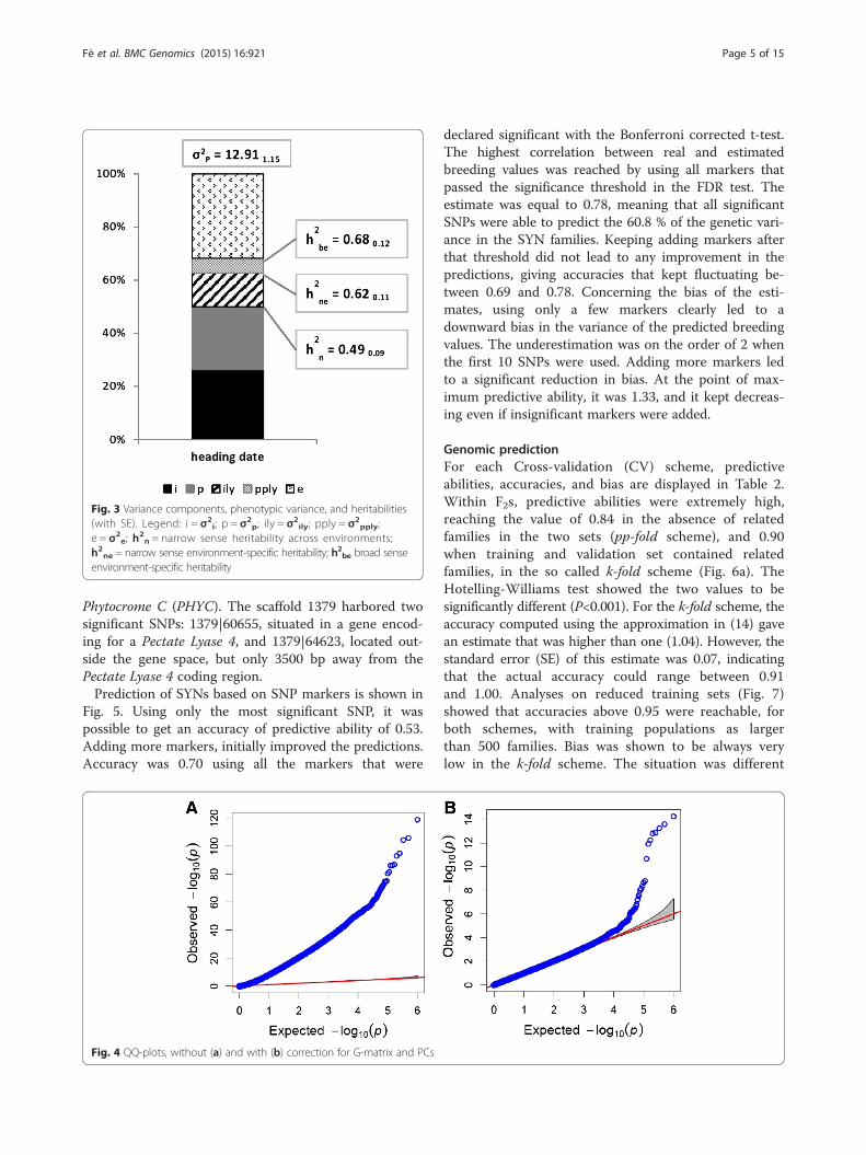
Fig. 3 Variance components, phenotypic variance, and heritabilities(with SE). Legend: i = σ2

i; p = σ2p; ily = σ2

ily; pply = σ2pply;

e = σ2e; h

2n = narrow sense heritability across environments;

h2ne = narrow sense environment-specific heritability; h2be broad senseenvironment-specific heritability

Fè et al. BMC Genomics (2015) 16:921 Page 5 of 15

Phytocrome C (PHYC). The scaffold 1379 harbored twosignificant SNPs: 1379|60655, situated in a gene encod-ing for a Pectate Lyase 4, and 1379|64623, located out-side the gene space, but only 3500 bp away from thePectate Lyase 4 coding region.Prediction of SYNs based on SNP markers is shown in

Fig. 5. Using only the most significant SNP, it waspossible to get an accuracy of predictive ability of 0.53.Adding more markers, initially improved the predictions.Accuracy was 0.70 using all the markers that were

Fig. 4 QQ-plots, without (a) and with (b) correction for G-matrix and PCs

declared significant with the Bonferroni corrected t-test.The highest correlation between real and estimatedbreeding values was reached by using all markers thatpassed the significance threshold in the FDR test. Theestimate was equal to 0.78, meaning that all significantSNPs were able to predict the 60.8 % of the genetic vari-ance in the SYN families. Keeping adding markers afterthat threshold did not lead to any improvement in thepredictions, giving accuracies that kept fluctuating be-tween 0.69 and 0.78. Concerning the bias of the esti-mates, using only a few markers clearly led to adownward bias in the variance of the predicted breedingvalues. The underestimation was on the order of 2 whenthe first 10 SNPs were used. Adding more markers ledto a significant reduction in bias. At the point of max-imum predictive ability, it was 1.33, and it kept decreas-ing even if insignificant markers were added.

Genomic predictionFor each Cross-validation (CV) scheme, predictiveabilities, accuracies, and bias are displayed in Table 2.Within F2s, predictive abilities were extremely high,reaching the value of 0.84 in the absence of relatedfamilies in the two sets (pp-fold scheme), and 0.90when training and validation set contained relatedfamilies, in the so called k-fold scheme (Fig. 6a). TheHotelling-Williams test showed the two values to besignificantly different (P<0.001). For the k-fold scheme, theaccuracy computed using the approximation in (14) gavean estimate that was higher than one (1.04). However, thestandard error (SE) of this estimate was 0.07, indicatingthat the actual accuracy could range between 0.91and 1.00. Analyses on reduced training sets (Fig. 7)showed that accuracies above 0.95 were reachable, forboth schemes, with training populations as largerthan 500 families. Bias was shown to be always verylow in the k-fold scheme. The situation was different

Table 1 Summary statistics for all the significant SNPs

Scaffold|Position Location MAF α % σ2g(F2) % σ2g(SYN) P-value Bonferroni P-value FDR

3546|38401 outside gene 0.08 1.19 1.62 0.65 6E-09 6E-09

18961|1999 exon 0.12 1.00 1.70 0.74 3E–08 1E–08

18961|3412 exon 0.27 0.57 1.01 0.71 0.004 4E–04

6570|54193 outside gene 0.11 1.03 1.68 1.02 6E–07 9E–08

22974|3466 outside gene 0.06 1.39 1.82 1.06 1E–06 2E–07

22974|2499 outside gene 0.22 0.74 1.47 0.86 2E–05 3E–06

1379|64623 outside gene 0.09 0.84 0.92 0.33 0.002 2E–04

1379|60655 exon 0.23 0.56 0.87 0.53 0.147 0.009

18588|6786 intron 0.06 1.14 1.19 0.37 0.002 2E–04

18588|6657 exon 0.28 0.50 0.79 0.52 0.417 0.020

18588|6882 exon 0.06 1.01 0.98 0.45 0.696 0.027

9291|22927 outside gene 0.18 0.59 0.80 0.46 0.007 6E–04

9679|461 outside gene 0.20 0.59 0.88 0.41 0.010 7E–04

2801|42855 exon 0.33 0.51 0.91 0.56 0.355 0.018

5059|6359 exon 0.25 0.51 0.77 0.53 0.457 0.021

3169|35325 exon 0.06 1.05 0.90 0.75 0.503 0.022

21110|2619 outside gene 0.17 0.52 0.59 0.28 0.597 0.025

3586|39964 exon 0.43 0.40 0.61 0.43 0.730 0.027

3395|30371 outside gene 0.39 0.47 0.82 0.54 0.837 0.030

Fè et al. BMC Genomics (2015) 16:921 Page 6 of 15

in the pp-fold CV, where the GEBVs variance wasgenerally underestimated, and where an increase inthe population size resulted in a bias reduction: theregression coefficient (b) was 1.39 using 175 families,and 1.10 using the full dataset. Bias for populationsizes below 175 families is not shown, because af-fected by very large SE and not indicative of anytrend. Accuracies within the set (UK) were lowerthan the ones found on an equal number of ran-domly chosen F2s, especially in the pp-fold scheme.Bias was also slightly higher. The CV within the

Fig. 5 Accuracies (a) and bias (b) for prediction of SYNs, based on marker effBonferroni corrected t-test (dotted line), and FDR (dashed line)

other cluster gave more or less the same results asthe CV within all F2s.Predictions across sets also worked well. Accuracy of

predicting UK set from the other F2 families was slightlylower (accuracy equal to 0.78). Predictions for GEBVswere better when the set (UK) was used as training set.In this case, accuracies were comparable to the ones ob-tained within all F2s, with a pp-fold scheme, and using asimilar population size. The bias level indicates that theGEBVs variance was underestimated when the set(UK) was used as training population, and slightly

ects. Legend: the vertical lines indicate the two significant thresholds:

Table 2 Population size and results (with SE) for all CV schemes

CV scheme Pop.size ρӯf;ĝ† ρg;ĝ bias (b)

k-fold 1757 0.90 0.01a 1.04 0.07 1.02 0.01

pp-fold 1757 0.84 0.01b 0.98 0.06 1.10 0.02

k-fold (UK) 466 0.78 0.03a 0.86 0.09 1.06 0.04

pp-fold (UK) 466 0.52 0.04b 0.57 0.07 1.30 0.10

k-fold (others) 1291 0.90 0.01a 1.04 0.07 1.02 0.01

pp-fold (others) 1291 0.86 0.01b 0.99 0.07 1.17 0.02

UK - > others 466 0.78 0.02N 0.90 0.07 1.46 0.03

Others - > UK 1291 0.71 0.03N 0.78 0.08 0.92 0.04

F2s - > SYNs (GS) 1757 0.88 0.05a 0.93 0.24 1.02 0.06

F2s - > SYNs (GWAS)‡ 1757 0.74 0.07b 0.78 0.21 1.33 0.13

†different letters indicate a significant difference between the two CV schemes(P < 0.001) based on Hotelling-Williams test. N indicates that the comparisondoes not apply, as models were based on different sets of data‡using all SNPs that were declared significant after FDR test

Fè et al. BMC Genomics (2015) 16:921 Page 7 of 15

overestimated when the prediction was performed inthe opposite direction. Predictive ability for SYNs(Fig. 6b) was similar to the ones within all F2s, andsignificantly different from the one obtained fromGWAS results (P< 0.001). The accuracy was 0.93,14 % higher than the in prediction based on the sig-nificant markers. In this case, the linear regression ofmean corrected phenotypes on GEBVs indicated nobias in the GEBVs variance.

DiscussionPopulation structure, LD, and genetic parametersThe population structure was mainly defined by the ori-gin of the PPs, which was correlated with the first prin-cipal component. The majority of the F2 families weregrouped in one big cluster. This may lead to the hypoth-esis of a common European genetic pool. This pool islikely to originate from the continuous and (more orless) free exchange of breeding material among the dif-ferent breeders. The parents of the set (UK) may be an

Fig. 6 GEBV vs. corrected mean phenotypes: a within F2s (k-fold); b predictline = linear regression

exception to that pool, and their genetic origin need tobe further investigated. The relation between PC3 andHD indicates the need to correct for population struc-ture while performing GWAS, in order to avoid falsepositives. Further variance analyses were performed byadding fixed regressions for the first 1, 2, 3, and 4 PCsto the equation shown in formula (2). Result indicates acorrelation of HD with the PC3, but not with the otherthree main PCs. When accounting for the first two PCs,the additive genomic variance across location was equalto the 98 % of the ones of the model without any PC.When accounting for the first three PCs, the additivegenetic variance left was the 89 %. Adding a regressionfor PC4 had a negligible effect.The LD within scaffolds showed to decay rapidly, con-

firming the concerns expressed by Hayes et al. [42], whoreported useful LD (r2 > 0.25) to extend at best 1 kb.However, in the present breeding material, the presenceof relatedness and population structure generally in-creased the LD, bringing to an increase by the order ofthree in the average distance between those markers.This fact suggests that population structure, which isknown to be mostly responsible for the long range LD,also plays an important role in increasing the level of LDwithin scaffolds. The correction also led to a decrease inthe average distance between markers in LD, which wasmore pronounced for higher LD levels.Estimation of variance components confirm results

obtained by Fè et al. [12] on a subset of the same data.In this paper was also possible to calculate the heritabil-ity across environments, and to estimate the extent ofG × E for additive and non-additive effects. Comparedwith other traits previously analyzed [12], the proportionof genetic variance between PPs was much higher. Thesmall level of G × E seems to confirm the results ob-tained by Ravel and Charmet [16]. However, plants werecultivated only in Denmark and England. To have a bet-ter understanding of G × E effects, it would be a good

ing SYNs from F2s. Legend: blue line = plot diagonal; red

Fig. 7 Accuracies (a) and bias (b) with different population sizes: k-fold (black) and pp-fold scheme (grey)

Fè et al. BMC Genomics (2015) 16:921 Page 8 of 15

idea to perform experiments covering more diverse cli-matic conditions. The significant amount of σ2pply mayindicate the presence of dominance acting between fam-ilies and within single environments. In the literature,the presence of non-additive effect is reported alsoacross location [15]. However results are not directlycomparable, as this paper ignores additive effects thatmay be present within F2 families.

Significant markers and genetic architectureThe GWAS analysis revealed a rather complex geneticarchitecture of HD in ryegrass. Several markers with sig-nificant effect were identified. In the most significantSNPs, a shift from one homozygous form to the othercan cause changes of up to 2.78 days in the date of head-ing. That is a remarkable difference, if compared withthe level of variation in the phenotypes: average pheno-types corrected for fixed effect had a SD of 4.92. How-ever, due to low Minor Allele Frequency (MAF), thesemarkers were only able to explain a small proportion ofthe additive variance, which may indicate the presenceof a large number of genes also affecting the trait, butwith effects lower than the detection limit. There were ahigh number of significant SNPs found outside the genespace. This is not too surprising considering a recentstudy in maize found that the majority of trait associatedvariants were located outside annotated genes, butwithin 5 Kb of transcriptional start and stop sites [43].Some of the significant SNPs were clearly linked to

genes that may have a direct or indirect influence onHD. It is well established that CONSTANS (CO) plays acrucial role in promoting flowering in response to longdays [44]. We identified a significant SNP within lessthan 5 Kb of a CO homolog. It has already been estab-lished that a ryegrass homolog to CO exhibits expressionpatterns consistent with its function in Arabidopsis, andcan complement co mutants [17]. Furthermore, the CO

homolog co-located on linkage group seven with a largeeffect QTL for HD [19, 31]. Allelic variation in an inter-genic region upstream of CO was found to be signifi-cantly associated with HD in a collection of 96 perennialryegrass genotypes (originating from nine populations)[32]. The ~29 Kb region sequenced as part of that studyshares near perfect identity with scaffold 5059 (Additionalfile 4: Figure S2), which has the significant SNP identifiedin our study, and therefore represent the same genomicregions. Overall, our results provide further evidencethat allelic variation at CO contributes to variation inHD in perennial ryegrass, specifically within a largecollection of breeding families.We also identified a significant SNP within the coding

region of a homolog to PHYC. Phytochromes are red/far-red photoreceptors that play a role in how a plant re-sponds to light, and adapts its growth and development.It was recently demonstrated in wheat that PHYC playsa major role in accelerating flowering under long-days[45], in contrast to the model plants such as Arabidopsisand rice where PHYC represses flowering under non-inductive conditions. The fact that loss-of-function mu-tations in PHYC resulted on average in a 108 day delayin flowering of wheat under long days emphasizes thepotential for allelic variation at this gene to greatly alterflowering times. A similar role for PHYC has also beenrecently reported in Brachypodium distachyon [46]. Per-ennial ryegrass is a close relative of wheat and Brachypo-dium, and a similar role for PHYC in floral induction ofperennial ryegrass is possible. A homolog to PHYC hasbeen mapped to linkage group four of perennial ryegrass[47], although it mapped some distance from the HDQTL identified in that experimental population. No cor-relation was found between significant markers andother genes that are known to be important in floweringtime regulation, such as FT. That may be due to differ-ent reasons: (i) absence of causative polymorphisms in

Fè et al. BMC Genomics (2015) 16:921 Page 9 of 15

the breeding material; (ii) no or low LD betweenmarkers and the causative polymorphisms (likely to hap-pen, due to the fast decaying LD); (iii) low MAF at thecausative polymorphisms (about 45 % of the markershad MAF lower than 0.05); (iv) polymorphisms not de-tected because they are correlated with the family struc-ture and shrunken by the correction with G-matrix andPCs (the third PC was clearly correlated with HD).

Prediction of breeding valuesDespite explaining only a small part of the genetic vari-ance in the SYNs, the significant markers were able topredict the breeding values with high accuracy, evenwhen only a few markers were used. This is due to fewgenes with relatively large effects identified in the F2population. However, the presence of a certain level ofpopulation structure (displayed in Fig. 1) will also con-tribute to the predictive ability in the SYNs. In theGWAS, we accounted for the presence of populationstructure by correcting the marker effect (using the G-matrix and the first four PCs). However, that correctiondoes not apply to the estimation of prediction accuracy.When we correlate the phenotypes with one marker, weare actually estimating the correlation of the phenotypewith that particular marker, plus all the populationstructure that is correlated to the SNP. The trend in ac-curacy for an increasing number of markers met our ex-pectations: any significant SNP is supposed to addinformation that will increase the correlation with thetrue breeding value. Non-significant SNPs will mainlyadd random noise to the correlation, but were able toadd genetic information that increased the variance ofestimated breeding values. The fact that the accuracyreaches the highest value in correspondence of the nine-teenth SNP is also a strong argument for using FDR, in-stead of Bonferroni corrected t-test, as significance test.The decreases in prediction accuracy that happenedafter adding the fourth and the sixth markers may be re-lated to different levels of expression or to different in-teractions in the two populations.Results from SYNs prediction (Table 2) show a clear

advantage for using GP, compared with GWAS, both interms of accuracies, and in terms of bias, as well as itsgood potential in predicting across different generations.The relatively high SE for accuracies may be related tothe experimental design that, due to incompleterandomization between trials and PPs, which could leadto less accurate estimate of PP variance components.Within all F2 families, predictions were extremely good,allowing the explanation of nearly the whole geneticvariance. This result is higher than what usually foundfor the same trait in other species (reviewed in [40]),even though accuracies above 0.8 have already been re-ported in other outcrossing species such as maize. That

may be related with the high level of structure in thepopulation, and to the fact that heading date primarily isaffected by additive genetic effects, so the additive valuesof the PPs are very well estimated.A very high accuracy may also seem in contrast with

what reported in the literature for traits affected bymajor effect SNPs [48]. Theoretically, for traits that in-clude some genes with large effect, it would be recom-mended to use other prediction methods such asBayesian models, which allow marker effects to belongto distributions with different variance. However, Gen-omic Best Linear Unbiased Prediction (GBLUP), whencompared with Bayesian methods, was shown to be bet-ter in accounting for population structure, but less cap-able to explain the short range LD between markers[36]. This makes it particularly effective for GP in breed-ing programs of species like perennial ryegrass, charac-terized quick decay of short range LD, and usually bredon a sib-mating scheme. The lower accuracies foundwithin the set (UK) may be related to a low level ofpopulation structure within the cluster, as appear alsofrom Fig. 1.Accuracies reached by predicting from related families

(k-fold scheme) were significantly higher than the onesobtained in the absence of related families (pp-foldscheme), for any population size. Regarding the relation-ship between predictions and the size of training popula-tion, increasing the training size led to pronounced gainsin predictive abilities for population sizes lower than 500families, and to smaller gains in the case of larger popu-lations. Despite that, due to the higher predictive abil-ities, accurate predictions could be obtained even usinga relatively small training set. Problems of underestima-tions of the GEBVs variance may arise in absence ofclosely related families. Regarding predictions acrosssets, the relative difficulty in predicting the set (UK) maybe due to families in this set having fewer relatives inthe chosen training population. The level of bias mayarise due to the differences in genetic variance or to gen-etic correlations that are less than unity between the twosets. This problem could compromise a correct compari-sons between GEBVs from the training set (which haveknown bias) and the validation set (which have unknownbias). This should be taken into consideration during thedesign of the training population, allowing the presencea wide variety of genotypes in as many environments aspossible.

ConclusionsOur research clearly showed considerable potential forimplementation of GS in breeding of L. perenne. Resultsobtained by GP significantly outperformed the accuracybased on traditional MAS, being able to predict a verylarge proportion of the genetic variance. GBLUP was

Fè et al. BMC Genomics (2015) 16:921 Page 10 of 15

shown to be capable of reaching very high accuracies,even in a trait characterized by major effect genes, atleast in a population with fast decaying LD and popula-tion structure arising from admixture and relatedness.Predictions were also very good across datasets, with ac-curacies of up to 0.93. Bias in the GEBV variance couldbe caused by lack of common parent populations be-tween training and validation set.The study has also revealed important details about

the genetic architecture of HD in L. perenne. The traitappears to be controlled by both major and minor effectgenes, regulated both by sequence changes within cod-ing regions, and by the action of intergenic regulatory el-ements. SNPs were identified within or proximal togenes with well-established roles in floral induction inplants (CONSTANS and PHYC). Despite this, the tech-nique used for GWAS has limitations, mainly due to themarker density given the rapid decay of LD, and due tothe strong structure in the population.

MethodsPlant material, genomic and phenotypic dataBoth Phenotypic and genomic data were available for atotal of 1846 families of forage diploid perennial rye-grass. All breeding material was part of a standard foragebreeding program run by DLF A/S (Store Heddinge,Denmark). Unlike cereal breeding, population based for-age breeding usually does not advance further than thesecond generation. Each year, the best breeding materialis selected and added to the company’s gene bank, whichalso includes European varieties, commercialized bothby DLF and other companies.The plant material consisted of two different sets:

Set 1. F2s: 1757 F2 families produced across 13 years(between 2000 and 2012) from a seed bank of 198 PPs.Development of F2 families was detailed in Fè et al.[12]. In brief: (i) pair-crosses between single plantsfrom two different PPs (self-pollination avoided due toself-incompatibility). Each single plant was used only inone pair-cross; (ii) seed harvesting from both parentplants; (iii) pooling of the F1 seeds; (iv) isolatedmultiplication of F1 populations in isolated plots forrandom mating; (v) harvesting of F2 seeds; (vi) fieldtrials of F2 families (assumed to be in Handy-Weinbergequilibrium).Set 2. SYNs: 89 families obtained by random matingbetween 5–11 single plants. Single plants were selectedfrom the highest biomass yielding F2 families, by visualmerits and according to the synchronous heading time.After crossing, SYNs production followed the sameprotocol described for F2 families, involving pooling,multiplication of the seed in isolated plots, and testingin field trials.

Sequence data was produced by Genotyping-By-Sequencing (GBS) [49]. GBS uses methylation sensitiverestriction enzymes (such as ApeKI) to target the lowcopy fraction of the genome, and can be used to esti-mate genome-wide allele frequency profiles in breedingpopulations [50]. Sampling and library preparationfollowed the protocol described by Byrne et al. [50], andElshire et al. [49]. A total of 32 libraries were prepared,each of them containing up to 64 F2 families, and se-quenced on multiple lanes of on an Illumina HiSeq2000(single-end). After basic data filtering, the average num-ber of reads per family was about 20 million. Data foreach family was then aligned against a draft sequence as-sembly. 1,879,139 SNPs were identified, distributedacross 30,285 scaffolds. Sequencing depth at a SNPranged from 1 to 250 (upper limit) reads per family.SNP positions having more than 60 reads were dis-carded, as suspected to be originated from plastid ge-nomes or from highly repetitive regions not captured inthe draft assembly. No threshold was set in relation tothe minimum number of reads. That could lead to apoor estimation of the allele frequencies and, conse-quently, to underestimation of allele substitution effect.However, it is possible to take account of this problemsby using specific corrections, as showed by Ashraf et al.[51]. Markers were also filtered based on allele frequen-cies, removing SNPs with an estimated MAF lower than0.02. After that, a total 1,447,122 markers were availablefor analyses. A further filtering was performed forGWAS and LD analyses (MAF > 0.05), leaving a total of1,005,590 SNPs.Phenotypic data were collected, within the standard

breeding procedures of DLF. Families were sown duringspring and scored during the following season. HD wasassessed on family means by visual scoring, and definedas the day in which, two-thirds of the spike is visible onat least one plant in the plot or one third of the spike isvisible in three plants in the plot. The character wasexpressed as ‘days after May 1st’. Data were available fora period of 11 years (between 2003 and 2013), and fortwo locations: Store Heddinge (South-Eastern Denmark)and Didbrook (Southern England). Fields were dividedin trials, each consisting of randomized 24 sward plots,arranged in 2 sub-trials. Plot size was 1.5*10 m inDenmark and 0.5*4 m in England. Randomization wasensured within trials, but not always across trials. Insome cases, especially in the oldest experiments, familieswere sorted according to the flowering time, or to theyear of origin. That resulted in a certain degree ofunbalance, within locations, between trials and PPs. Asummary of the phenotypic data is displayed inTable 3, which shows the number of phenotyped families,along with the number of environments (location × year)where data were recorded, and some descriptive

Table 3 Summary statistics for F2 and SYN families

F2s SYNs

N. phenotyped families 1757 89

N. locations 2 2

N. environments (location*year) 10 4

N. replicates 3.9 2.3

N. location per family 1.56 1.18

N. environments per family 1.98 1.18

Mean 25.9 31.5

SD 8.6 8.6

Min 3 13

Max 51 50

Fè et al. BMC Genomics (2015) 16:921 Page 11 of 15

statistics (mean, standard deviation [SD], minimum,and maximum).

Population Structure and LDA Genomic relationship matrix (G-matrix) for all fam-ilies was calculated from all SNP markers, after filteringfor SNP depth and allele frequency (MAF > 0.02). Firstly,allele frequencies were arranged in a matrix X(i×j), with iindexing marker, and j indexing family. The matrix wasthen centered by mean SNP frequencies Mij ¼ Xij−�Xi

� �,

where missing data were imputed with the average allelefrequency, and used to compute G:

G ¼ M′M=K ð1Þwhere K is a scaling parameter, corresponding to thesum of expected SNP variances as computed by Ashraf

et al. [51], being 0.25XNi¼1

�Xi 1−�Xið Þ, with N equal to num-

ber of markers. Then, a PCA was performed on the G-matrix. The best number of clusters was determined by k-means clustering, using the R package ‘NbClust’ [52]. Theprobability, for each family, to belong to each cluster wascomputed with the R package ‘e1071’ [53]. LD within scaf-folds was measured across all the F2 families on a set of 100scaffolds larger than 20 kbp, randomly sampled across thewhole genome. The LD was expressed as squared correl-ation between markers (r2). Corrections for both related-ness and for population structure were performedaccording to the method described by Mangin et al. [54].

Statistical models and genetic parametersData were analyzed by linear mixed models, using thesoftware DMU [55, 56]. The genomic information wasimplemented by using the G-matrix as variance covari-ance structure of the breeding values. Due to the notperfectly randomized design, the trial effect was includedin the fixed part of the model [57]. Different modelswere tested on the F2 set and compared by F-test (for

the fixed part) and Akaike test (for the random part).The models that showed the best fit to the data is re-ported below:

y ¼ Xtþ Z1iþ Z2ily þ Z3pþ Z4pply þ e ð2Þwhere y is the vector of phenotypes; X is the designmatrix for the fixed factor; t is the vector of trial effectsnested within location and year; Zi are design matricesfor random factors; i is a vector of breeding values ~N(0, Gσ2i ), where G is the G-matrix; ily is a vector ofgenotype × environment interactions ~ N(0, Iσ2ily); p is avector of the originating PPs ~ N(0, Pσ2p), with P beinga genomic relationship matrix among PPs (P-matrix)built as described in the following paragraph; pply isthe vector of interaction between PPs (which wouldmainly arise from dominance effects) nested withinenvironments ~ N(0, Iσ2pply); e is a vector of randomresiduals ~ N(0, Iσ2e). Additional factors for breedingvalues and PPs, with identity matrices as variance-covariance structure were tested to check for presenceof genetic effects not explained by G- and P- matrix.However, such effects turned out to be not significantlydifferent from zero and were left out from the model. Thesame was for the interactions among PPs and betweenPPs and environments, and for the spatial effectwithin trials. Breeding values were calculated by summingthe corresponding solutions for i and p:

gj ¼ ij þ p j1þ pj2

ð3Þwhere j indicates family and j1 and j2 indicates the par-ents population for family j.Matrix Z3 was built to account for the presence of

multiple PPs, as shown in Additional file 5: Figure S3 inthe supplementary material. In each row, numbers indi-cate the expected probability, for each allele, to comefrom each PP. As each locus has two alleles, the num-bers on each row sum up to two. P was computed basedon the estimated frequencies of the PPs, following thesame procedure that used to compute G-matrix. PPs fre-quencies were estimated for each SNP marker, using thefollowing model:

f i ¼ μi þ Zpi þ ei ð4Þwhere fi is the vector of frequencies for marker i; μi isthe mean frequency for marker i; Z is a matrix of ran-dom effect, accounting for the presence of multiple PPs,built as explained in Additional file 5: Figure S3; pi is avector of originating PPs ~ N(0, Iσ2p). The estimated PPsfrequency for a marker i was equal to:

fpi ¼ μi þ 2pi ð5ÞThe model was based on the additive biallelic infini-

tesimal model described by Ashraf et al. [51], which was

Fè et al. BMC Genomics (2015) 16:921 Page 12 of 15

built on the following assumptions: (i) large number ofindividuals in PPs, F1 and F2 families; (ii) PPs in Hardy-Weinberg equilibrium; (iii) large number of familiesoriginated by each parent combination; (iv) parent plantschosen at random from the PPs; (v) absence of self-pollination; (vi) no intercross among F1 families; (vii)absence of selection between F1s and F2s; (viii) uniform var-iances across different factors. Here, the only difference inrespect to the original model is represented by the relation-ship among PPs. That would cause inbreeding between theF1’s, [51] and lead to changes in frequencies and variancesamong PPs and F2s (described by P-matrix and by G-matrix respectively), and within F2s. The latter componentcan be ignored, as analyses are based on family means. TheG-matrix also accounts for the increase in inbreedingwithin the F2 families. Variance components were estimatedby restricted maximum likelihood method (REML), andcan be interpreted as follows: σ2i is the additive geneticvariance among families, across environments; σ2ily is theadditive G × E variance; σ2p is the variance among PPsacross environments; σ2pply is the variance of the G× E fordominance; σ2e is the variance of residuals, which includesenvironmental effects within plots and measurement errors.Across PPs, it was possible to compute three kinds

of heritabilities for a single observation: (6) narrowsense heritability across environments; (7) narrowsense environment-specific heritability; (8) broad senseenvironment-specific heritability:

h2n ¼ Gσ2

i þ 2Pσ2p

� �=σ2

P ð6Þ

h2ne ¼ Gσ2

i þ 2Pσ2p þ σ2

ily� �

=σ2P ð7Þ

h2be ¼ Gσ2

i þ 2Pσ2P þ σ2

ily þ σ2pply

� �=σ2

P ð8Þwhere the component σ2p was added twice, as each F2family was originated from two PPs, and where σ2P is thephenotypic variance, calculated as:

σ2P ¼ Gσ2

i þ σ2ily þ 2Pσ2

p þ σ2pply þ σ2

e: ð9Þ

Genome Wide Association and Genomic PredictionGWAS analysis was performed by using the softwareGAPIT [58]. Correction for relatedness was ensured by theuse of G-matrix as kinship matrix. A further correction forpopulation structures was carried out by adding the mainfour PCs to the model. The optimal number of PCs was de-termined by GAPIT through Bayesian Information Criter-ion. The model used for GWAS was the following:

g ¼ X1α0i þ X2pcþ Ziþ e ð10Þwhere ĝ is a vector of breeding values, calculated fromthe model shown in equation (3), but assuming all vari-ance covariance matrices to be identity matrices; Xi and

Z are design matrices for fixed and random effects re-spectively; α0i is the allele substitution effect for locus i;pc is the vector for PCs effects; i is the vector of breed-ing values with G-matrix as variance-covariance struc-ture distributed as N(0, Gσ2i); e is a vector of randomresiduals, distributed as N(0, Iσ2e). Missing genotypes,for each marker, were imputed with the average allelefrequencies across families, as was done for computingG-matrix. The significance of each marker effect wasevaluated using t-test after Bonferroni correction andFDR [59], using a cut off level of 0.05. In case there weretwo or more significant markers in the same scaffold, anLD analyses was performed within the scaffold. WhenSNPs were in LD (r2 > 0.10), only the marker with thelowest P-values was regarded as significant. Allele substi-tution effects were corrected for low sequencing depth[51], using the following formula:

αi ¼ α0i � 1þ 3=Dið Þ ð11Þwhere α0 is the allele substitution effect as estimatedfrom GWAS, α is the corrected allele substitution effect,D is the average sequencing depth across families, and irefers to a given locus.As the allele frequencies are expressed on family

means, the genetic variance would be half of the vari-ance between individuals [51], and the variance ex-plained by each marker should be computed with thefollowing formula:

σ2gi ¼ pi 1−pið Þαi2 ð12Þ

where p is the MAF, α is equal to the allele substitutioneffect, and i refers to a given allele. For all the SNPs thatwere declared significant in at least one of the tests, σ2giwas calculated both within the F2 families, and using theMAF of the SYN families. Then, a single marker regres-sion was performed in the SYN families, in order to checkthe association between marker effects in the two sets.Later, all SNPs were ordered based on their P-values, andthen used to estimate the GEBVs of the SYN families:

g¼ΣM

i¼1αi � pi ð13Þ

in this equation, ĝ is the vector of GEBVs, M is equal tothe number of significant markers, αi is the allele substi-tution effect for marker i, and pi is the MAF at markeri. The calculation was performed multiple times, assum-ing different values for M (from 1 to 50 markers).GP studies were carried out by GBLUP [60, 61], using

CV within different F2 sets: (i) all F2 families; (ii) differ-ent clusters of F2 families, previously identified duringthe PCA; (iii) reduced sets of randomly chosen F2s, dif-fering for size of the training populations. Within eachset, CV was performed according to two different

Fè et al. BMC Genomics (2015) 16:921 Page 13 of 15

schemes testing different hypothesis: (a) k-fold (k = 100)tests predictions in case of presence of related individ-uals in the training and in the validation set, leaving outfamilies in random order and estimates their breedingvalues; (b) pp-fold tests predictions in case of absence ofrelated individuals in the training and in the validationset, estimating all the families originated by a certainPPs combination, after having left out everything thathad at least a PP in common. As pp-fold implied agreater reduction in terms of training population com-pared to k-fold, a pp-like strategy was also tested, inorder to ensure the same training population size is usedin both schemes. This strategy exactly replicated thecross-validation scheme used in pp-fold, but leaving outrandom families instead. Analyses on set (iii) were re-peated ten times, each time using a different set of ran-domly chosen F2s, and the average predictive abilitiesand bias were calculated. Then, CVs were performedacross clusters and, finally, all the F2s were used to pre-dict the breeding values of the SYN families.Accuracy is defined as the correlation between true

breeding values and GEBVs (ρg,ĝ). In this case, its valueis not known, but can easily be computed by using thefollowing equation [62]:

ρg;g ¼ ρ�yf;g=ρ�yf ;g ð14Þ

where the nominator is the true correlation betweenGEBVs with the average phenotypes corrected for thefixed effect (yf ), defined as predictive ability, and the de-nominator represents the expected correlation betweenGEBVs and �yf . Such a formula gives an estimation of thecorrelation between g and ĝ, which is not guaranteed tofall within the theoretically defined range of the pa-rameters. The expected correlation between GEBVsand �yf can be calculated with the following equation[63]:

ρ�yf;g ¼ σg � σ2g þ σ2

e=n� �− 1=2ð Þ ð15Þ

where σ2g is the genomic variance, and n number ofreplicates. That is equivalent to the square root of theheritability based on family means (based on severalobservations), and represents the upper limit for theprediction accuracy. However, this formula refers to avery simplified model with only genomic and residualvariances. In the present paper, the equation needs toaccount for the other random components:

ρ�yf ;g ¼ffiffiffiffiffiffiffiffiffiffiffiffiffiffiffiffiffiffiffiffiffiffiffiffiffiffiffiffiGσ2

i þ 2Pσ2p

q� ðGσ2

i þ 2Pσ2p

þσ2ily=nily þ σ2

pply=npply þ σ2e=nÞ−ð1=2Þ

ð16Þ

As different families were replicated a different num-ber of times, n is the average number of replicates acrossall fields (nplots/nfamilies); nily is the average number of

environments per each family (nily/nfamilies) and npply is theaverage number of environments per each PP (nPPly/nPP).When predictions were performed on the same dataset,comparison between predictive abilities from differentmodels was performed with Hotelling-Williams test [64],using the R script developed by Christensen et al.[65]. The bias of the predictions was investigated byregressing �yf on the breeding value estimates:

�yf ¼ bg þ c; b ¼ σ�yf ;g=σ2g ð17Þ

where �yf is the vector of corrected and average pheno-types not included in computing GEBVs, and ĝ is thevector of GEBVs from the CV procedure. Absence ofbias will result in a regression coefficient (b) of 1. A sig-nificant deviation from 1 indicates bias in the estimationof the GEBVs’ variance.

Additional files

Additional file 1: Figure S1. PCA scree plot. (BMP 13 kb)

Additional file 2: Genes predicted in the scaffolds harboring thesignificant SNPs. (XLSX 14 kb)

Additional file 3: Table S1. Scaffolds with significant SNPs. (DOCX 14 kb)

Additional file 4: Figure S2. A dot plot of the sequence alignment ofthe genomic scaffold (first sequence) that contains the SNP significantlyassociated with heading date, and proximal to CO, against the 29Kbregion (SEQ2) sequenced in the study of Skøt et al., [29]. (BMP 2159 kb)

Additional file 5: Figure S3. Construction of the design matrices forPPs. Legend: F2_j, SYNj = families; PPi = parent populations. (BMP 288 kb)

Abbreviationsbp: base pairs; CV: cross-validation; FDR: false discovery rate; G × E: genotype byenvironment; GBLUP: genomic best liner unbiased prediction; GBS: genotypeby sequencing; GEBV: genomic estimated breeding value; GP: genomicprediction; GS: genomic selection; GWAS: Genome Wide Association Analysis;HD: heading date; LD: linkage disequilibrium; LG: linkage group; MAF: minorallele frequency; MAS: marker assisted selection; PP: Parent population;QTL: quantitative trait locus; SYN: synthetic familiy.

Competing interestsDario Fè is enrolled as an “Industrial PhD student” at Aarhus University and isemployed at DLF A/S. An industrial PhD student is working in a joint researchproject (run together buy a university and a private company). Public founding isalso provided by the Danish Ministry of Education, through the Council forIndustrial PhD Education (11–109967). Detailed info is available here: http://ufm.dk/en/research-and-innovation/funding-programmes-for-research-and-innovation/find-danishfunding-programmes/programmes-managed-by-innovation-fund-denmark/industrial-phd. The present project is also founded bythe Danish Ministry of Food, Agriculture and Fisheries, through The Law ofInnovation (3412-09-02602) and the GUDP (Grønt Udviklings- ogDemonstrationsprogram - Green Development and Demonstration Program)(3405-11-0241).Ingo Lenk, Morten Greve Pedersen, Niels Roulund and Christian Sig Jensenare employed by DLF A/S. The other authors declare that they have nocompeting interests.

Authors’ contributionsDF carried out the GP and GWAS analyses and had the major role in draftingthe manuscript. MGP and NR were involved in the production of the plantmaterial and in the acquisition of the phenotypic data. IL was involved inDNA sample preparation, sequencing and alignment. SB and TA carried outthe sequencing, and subsequent bioinformatics analysis, and played a majorrole in the interpretation and in the writing of the GWAS results. BA and LJ

Fè et al. BMC Genomics (2015) 16:921 Page 14 of 15

worked on the development of the statistical models and on thecomputation of the genetic relationship matrices. FC carried out in the PCAand LD analysis and was involved in the computation of the geneticrelationship matrices. CSJ played a major role in the interpretation of dataand in drafting the manuscript. JJ worked on the development of thestatistical models, on the interpretation of data, and on drafting themanuscript. All authors read and approved the final manuscript.

AcknowledgmentsThe project was financed by the Danish Ministry of Education, through theCouncil for Industrial Ph.D. Education (11–109967), by the Danish Ministry of Food,Agriculture, and Fisheries, through The Law of Innovation (3412-09-02602) andthe Green Development and Demonstration Program (GUDP; 3405-11-0241),and by DLF A/S.We also acknowledge Adrian Czaban and Stephan Hentrup, who collaboratedon the preparation of GBS libraries, working at Aarhus University, Department ofMolecular Biology and Genetics, Crop Genetics and Biotechnology.

Author details1Department of Molecular Biology and Genetics, Center for QuantitativeGenetics and Genomics, Aarhus University, Blichers Allé 20, 8830 Tjele,Denmark. 2Department of Molecular Biology and Genetics, Crop Geneticsand Biotechnology, Aarhus University, Forsøgsvej 1, 4200 Slagelse, Denmark.3DLF A/S, Research Division, Højerupvej 31, 4660 Store Heddinge, Denmark.

Received: 27 May 2015 Accepted: 29 October 2015

References1. Wilkins PW. Breeding perennial ryegrass for agriculture. Euphytica. 1991;52:201–14.2. Fulkerson W, Slack K, Lowe K. Variation in the response of Lolium genotypes

to defoliation. Aust J Agric Res. 1994;45(Alberda 1966):1309–17.3. Tallowin JRB, Brookman SKE, Santos GL. Leaf growth and utilization in four

grass species under steady state continuous grazing. J Agric Sci.1995;124:403–17.

4. Cornish MA, Hayward MD, Lawrence MJ. Self-incompatibility in ryegrass I.Genetic control in diploid Lolim perenne L. Heredity (Edinb). 1979;43:95–106.

5. Yano M. Naturally occurring allelic variations as a new resource forfunctional genomics in rice. In: Khush GS, Brar DS, Hardy B, editors. RiceGenet IV. Enfield: Science Publishers, Inc.; 2001. p. 227–238.

6. Emebiri LC, Moody DB. Heritable basis for some genotype-environment stability statistics: Inferences from QTL analysis ofheading date in two-rowed barley. F Crop Res. 2006;96:243–51.

7. Yamada T, Jones ES, Cogan NOI, Vecchies a C, Nomura T, Hisano H, et al.QTL analysis of morphological, developmental, and winter hardiness-associated traits in perennial ryegrass. Crop Sci. 2004;44:925–35.

8. Studer B, Jensen LB, Hentrup S, Brazauskas G, Kölliker R, Lübberstedt T.Genetic characterisation of seed yield and fertility traits in perennial ryegrass(Lolium perenne L.). Theor Appl Genet. 2008;117:781–91.

9. Humphreys MO. A genetic approach to the multivariate differentiation ofperennial ryegrass (Lolium perenne L.) populations. Heredity (Edinb).1991;66:437–43.

10. Laidlaw a S. The relationship between tiller appearance in spring andcontribution to dry-matter yield in perennial ryegrass (Lolium perenne L.)cultivars differing in heading date. Grass Forage Sci. 2005;60:200–9.

11. Sampoux JP, Baudouin P, Bayle B, Béguier V, Bourdon P, Chosson JF, et al.Breeding perennial grasses for forage usage: an experimental assessment oftrait changes in diploid perennial ryegrass (Lolium perenne L.) cultivarsreleased in the last four decades. F Crop Res. 2011;123:117–29.

12. Fè D, Pedersen MG, Jensen CS, Jensen J. Genetic and EnvironmentalVariation in a Commercial Breeding Program of Perennial Ryegrass. Crop Sci.2015;55:631.

13. Bugge G. Selection for seed yield in Lolium perenne L. Plant Breed.1987;98:149–55.

14. Elgersma A. Spaced-plant traits related to seed yield in plots of perennialryegrass (Lolium perenne L.). Euphytica. 1990;51:151–61.

15. Kearsey MJ, Hayward MD, Devey FD, Arcioni S, Eggleston MP, Eissa MM.Genetic analysis of production characters in Lolium 1. Triple test crossanalysis of spaced plant performance. J Agric Sci. 1987;75:66–75.

16. Ravel C, Charmet G. A comprehensive multisite recurrent selection strategyin perennial ryegrass. Euphytica. 1996;88:215–26.

17. Martin J, Storgaard M, Andersen CH, Nielsen KK. Photoperiodic regulation offlowering in perennial ryegrass involving a CONSTANS-like homolog. PlantMol Biol. 2004;56:159–69.

18. Yamada T, Forster JW, Humphreys MW, Takamizo T. REVIEW. Genetics andmolecular breeding in Lolium/Festuca grass species complex. Grassl Sci.2005;51:89–106.

19. Andersen JR, Jensen LB, Asp T, Lübberstedt T. Vernalization response inperennial ryegrass (Lolium perenne L.) involves orthologues of diploidwheat (Triticum monococcum) VRN1 and rice (Oryza sativa) Hd1. Plant MolBiol. 2006;60:481–94.

20. Laurie D a. Comparative genetics of flowering time. Plant Mol Biol.1997;35:167–77.

21. Jensen CS, Salchert K, Nielsen KK. A TERMINAL FLOWER1-like gene fromperennial ryegrass involved in floral transition and axillary meristem identity.Plant Physiol. 2001;125:1517–28.

22. Andersen CH, Jensen CS, Petersen K. Similar genetic switch systems mightintegrate the floral inductive pathways in dicots and monocots. TrendsPlant Sci. 2004;9:105–7.

23. Petersen K, Didion T, Andersen CH, Nielsen KK. MADS-box genes fromperennial ryegrass differentially expressed during transition from vegetativeto reproductive growth. J Plant Physiol. 2004;161:439–47.

24. Jones ES, Mahoney NL, Hayward MD, Armstead IP, Jones JG, HumphreysMO, et al. An enhanced molecular marker based genetic map of perennialryegrass (Lolium perenne) reveals comparative relationships with otherPoaceae genomes. Genome. 2002;45:282–95.

25. Armstead IP, Turner LB, Farrell M, Skøt L, Gomez P, Montoya T, et al. Syntenybetween a major heading-date QTL in perennial ryegrass (Lolium perenneL.) and the Hd3 heading-date locus in rice. Theor Appl Genet.2004;108:822–8.

26. Jensen LB, Andersen JR, Frei U, Xing Y, Taylor C, Holm PB, et al. QTLmapping of vernalization response in perennial ryegrass (Lolium perenne L.)reveals co-location with an orthologue of wheat VRN1. Theor Appl Genet.2005;110:527–36.

27. Armstead IP, Turner LB, Marshall a H, Humphreys MO, King IP,Thorogood D. Identifying genetic components controlling fertility in theoutcrossing grass species perennial ryegrass (Lolium perenne) byquantitative trait loci analysis and comparative genetics. New Phytol.2008;178:559–71.

28. Barre P, Moreau L, Mi F, Turner L, Gastal F, Julier B, et al. Quantitative traitloci for leaf length in perennial ryegrass (Lolium perenne L.). Grass ForageSci. 2009;64:310–21.

29. Byrne S, Guiney E, Barth S, Donnison I, Mur L a J, Milbourne D. Identificationof coincident QTL for days to heading, spike length and spikelets per spikein Lolium perenne L. Euphytica. 2009;166:61–70.

30. Shinozuka H, Cogan NOI, Spangenberg GC, Forster JW. Quantitative TraitLocus (QTL) meta-analysis and comparative genomics for candidate geneprediction in perennial ryegrass (Lolium perenne L.). BMC Genet.2012;13:101.

31. Armstead IP, Skøt L, Turner LB, Skøt K, Donnison IS, Humphreys MO,et al. Identification of perennial ryegrass (Lolium perenne (L.)) andmeadow fescue (Festuca pratensis (Huds.)) candidate orthologoussequences to the rice Hd1(Se1) and barley HvCO1 CONSTANS-likegenes through comparative mapping and microsynteny. New Phytol.2005;167:239–47.

32. Skøt L, Humphreys J, Humphreys MO, Thorogood D, Gallagher J, SandersonR, et al. Association of candidate genes with flowering time and water-soluble carbohydrate content in Lolium perenne (L.). Genetics.2007;177:535–47.

33. Corbesier L, Vincent C, Jang S, Fornara F, Fan Q, Searle I, et al. Long-distancesignaling in floral induction of Arabidopsis. Science (80- ). 2007;316:1030–3.

34. Tamaki S, Matsuo S, Wong HL, Yokoi S, Shimamoto K. Hd3a protein is amobile. Science (80- ). 2007;316:1033–6.

35. Skøt L, Sanderson R, Thomas A, Skøt K, Thorogood D, Latypova G, et al.Allelic variation in the perennial ryegrass FLOWERING LOCUS T gene isassociated with changes in flowering time across a range of populations.Plant Physiol. 2011;155:1013–22.

36. Jannink J-L, Lorenz AJ, Iwata H. Genomic selection in plant breeding: fromtheory to practice. Brief Funct Genomics. 2010;9:166–77.

37. Beavis W. QTL analyses: power, precision, and accuracy. In: Paterson AH,editor. Molecular dissection of complex traits. New York: CRC Press;1998. p. 145–62.

Fè et al. BMC Genomics (2015) 16:921 Page 15 of 15

38. Xu S. Theoretical basis of the Beavis effect. Genetics. 2003;165:2259–68.39. Hayes BJ, Bowman PJ, Chamberlain a J, Goddard ME. Invited review:

Genomic selection in dairy cattle: progress and challenges. J Dairy Sci.2009;92:433–43.

40. Lin Z, Hayes BJ, Daetwyler HD. Genomic selection in crops, trees andforages : a review. Crop pasture Sci. 2014;65:1177–91.

41. Heffner EL, Lorenz AJ, Jannink JL, Sorrells ME. Plant breeding with genomicselection: gain per unit time and cost. Crop Sci. 2010;50:1681–90.

42. Hayes BJ, Cogan NOI, Pembleton LW, Goddard ME, Wang J, SpangenbergGC, et al. Prospects for genomic selection in forage plant species. PlantBreed. 2013;132:133–43.

43. Wallace JG, Bradbury PJ, Zhang N, Gibon Y, Stitt M, Buckler ES. Associationmapping across numerous traits reveals patterns of functional variation inmaize. PLoS Genet. 2014;10:e1004845.

44. Putterill J, Robson F, Lee K, Simon R, Coupland G. The CONSTANS gene ofArabidopsis promotes flowering and encodes a protein showing similaritiesto zinc finger transcription factors. Cell. 1995;80:847–57.

45. Chen A, Li C, Hu W, Lau MY, Lin H, Rockwell NC, et al. PHYTOCHROME Cplays a major role in the acceleration of wheat flowering under long-dayphotoperiod. Proc Natl Acad Sci U S A. 2014;111:10037–44.

46. Woods DP, Ream TS, Minevich G, Hobert O, Amasino RM. PHYTOCHROME Cis an essential light receptor for photoperiodic flowering in the temperategrass, Brachypodium distachyon. Genetics. 2014;198(September):397–408.

47. Studer B, Byrne S, Nielsen RO, Panitz F, Bendixen C, Islam M, et al. Atranscriptome map of perennial ryegrass (Lolium perenne L.). BMCGenomics. 2012;13:140.

48. De los Campos G, Hickey JM, Pong-Wong R, Daetwyler HD, Calus MPL.Whole-genome regression and prediction methods applied to plant andanimal breeding. Genetics. 2013;193:327–45.

49. Elshire RJ, Glaubitz JC, Sun Q, Poland J a, Kawamoto K, Buckler ES, et al.A robust, simple genotyping-by-sequencing (GBS) approach for highdiversity species. PLoS One. 2011;6:1–10.

50. Byrne S, Czaban A, Studer B, Panitz F, Bendixen C, Asp T. Genome WideAllele Frequency Fingerprints (GWAFFs) of Populations via Genotyping bySequencing. PLoS One. 2013;8.3:e57438.

51. Ashraf BH, Jensen J, Asp T, Janss LL. Association studies using family poolsof outcrossing crops based on allele-frequency estimates from DNAsequencing. Theor Appl Genet. 2014;127:1331–41.

52. Charrad M, Ghazzali N, Boiteau V, Niknafs A. NbClust : an R package fordetermining the relevant number of clusters in a data set. J Stat Softw.2014;61:1–36.

53. Meyer D, Dimitriadou E, Hornik K, Weingessel A, Leisch F, Chang C-C, et al.Misc functions of the Department of Statistics (e1071). 2015.

54. Mangin B, Siberchicot A, Nicolas S, Doligez A, This P, Cierco-Ayrolles C.Novel measures of linkage disequilibrium that correct the bias due topopulation structure and relatedness. Heredity (Edinb). 2012;108:285–91.

55. Jensen J, Mäntysaari E, Madsen P, Thompson R. Residual maximumlikelihood estimation of (co) variance components in multivariate mixedlinear models using average information. J Indian Soc Agric Stat.1997;49:215–36.

56. Madsen P, Jensen J. A users guide to DMU. A package for analysingmultivariate mixed models. 2013.

57. Henderson CR. Applications of Linear Models in Animal Breeding Models.1984.

58. Lipka AE, Tian F, Wang Q, Peiffer J, Li M, Bradbury PJ, et al. GAPIT: Genomeassociation and prediction integrated tool. Bioinformatics. 2012;28:2397–9.

59. Benjamini Y, Hochberg Y. Controlling the false discovery rate : a practicaland powerful approach to multiple testing. J R Stat Soc B. 1995;57:289–300.

60. Habier D, Fernando RL, Dekkers JCM. The impact of genetic relationshipinformation on genome-assisted breeding values. Genetics.2007;177:2389–97.

61. VanRaden PM. Efficient methods to compute genomic predictions. J DairySci. 2008;91:4414–23.

62. Su G, Madsen P, Nielsen US, Mäntysaari E a, Aamand GP, Christensen OF,et al. Genomic prediction for Nordic Red Cattle using one-step andselection index blending. J Dairy Sci. 2012;95:909–17.

63. Crossa J, De Los CG, Pérez P, Gianola D, Burgueño J, Araus JL, et al.Prediction of genetic values of quantitative traits in plant breeding usingpedigree and molecular markers. Genetics. 2010;186:713–24.

64. Dunn O, Clark V. Comparison of tests of the equality of dependentcorrelation coefficients. J Am Stat Assoc. 1971;66:904–8.

65. Christensen OF, Madsen P, Nielsen B, Ostersen T, Su G. Single-step methodsfor genomic evaluation in pigs. Animal. 2012;6:1565–71.

Submit your next manuscript to BioMed Centraland take full advantage of:

• Convenient online submission

• Thorough peer review

• No space constraints or color figure charges

• Immediate publication on acceptance

• Inclusion in PubMed, CAS, Scopus and Google Scholar

• Research which is freely available for redistribution

Submit your manuscript at www.biomedcentral.com/submit