1

Genetic Based Discrete Particle Swarm Optimization for Elderly Day

Care Center Timetabling

M.Y. LIN1, K.S. CHIN

2*, and K.L. TSUI

3, T.C. WONG

4,

1 Department of Systems Engineering and Engineering Management, City University of Hong Kong, Kowloon Tong,

Kowloon, Hong Kong, meiyanlin2-c@my.cityu.edu.hk

2 Department of Systems Engineering and Engineering Management and Centre of Systems Informatics Engineering,

City University of Hong Kong, Kowloon, Hong Kong, mekschin@cityu.edu.hk

3 Department of Systems Engineering and Engineering Management and Centre of Systems Informatics Engineering,

City University of Hong Kong, Kowloon, Hong Kong, kltsui@cityu.edu.hk

4 Department of Design, Manufacture, and Engineering Management, University of Strathclyde, Glasgow, Scotland,

United Kingdom, andywtc@graduate.hku.hk

Abstract

The timetabling problem of local Elderly Day Care Centers (EDCCs) is formulated into a

weighted maximum constraint satisfaction problem (Max-CSP) in this study. The EDCC

timetabling problem is a multi-dimensional assignment problem, where users (elderly) are

required to perform activities that require different venues and timeslots, depending on

operational constraints. These constraints are categorized into two: hard constraints, which must

be fulfilled strictly, and soft constraints, which may be violated but with a penalty. Numerous

methods have been successfully applied to the weighted Max-CSP; these methods include exact

algorithms based on branch and bound techniques and approximation methods based on repair

heuristics, such as the min-conflict heuristic. This study aims to explore the potential of

evolutionary algorithms by proposing a genetic-based discrete particle swarm optimization

(GDPSO) to solve the EDCC timetabling problem. The proposed method is compared with the

min-conflict random-walk algorithm (MCRW), Tabu search (TS), standard particle swarm

optimization (SPSO), and a guided genetic algorithm (GGA). Computational evidence shows that

GDPSO significantly outperforms the other algorithms in terms of solution quality and efficiency.

Keywords

Timetabling problem, discrete particle swarm optimization, weighted Max-constraint satisfaction

problem, Tabu search, genetic algorithm, min-conflict random walk

2

Abbreviations

ANOVA Analysis Of Variance

BCO Bee Colony Optimization

CSP Constraint Satisfaction Problem

DPSO Discrete Particle Swarm Optimization

EDCC Elderly Day Care Center

FSP Flow-Shop Scheduling Problem

GA Genetic Algorithm

GDPSO Genetic-based Discrete Particle Swarm Optimization

GGA Guided Genetic Algorithm

JSP Job Shop Scheduling Problem

Max-CSP Maximum Constraint Satisfaction Problem

MCRW Min-Conflict Random-Walk algorithm

NP-hard non-deterministic polynomial hard

PSO Particle Swarm Optimization

ROV Ranked-Order Value

SA Simulated Annealing

SPSO Standard Particle Swarm Optimization

TS Tabu Search

3

1. Introduction

Driven by fertility and mortality reduction, and medical and economic advancements, the rapid

aging of the world population has been one of the major global demographic trends [1]. This trend

has also increased the demand for age-friendly and affordable healthcare services, including the

long-term care, curative care and preventive care. Thus, the quality of healthcare services

provided by day-care centers, community care centers and nursing homes gains increasingly

significant attention [2]. To ensure the quality of such services, centers should deliver more

effective services. However, many care centers suffer from operational inefficiency. Driven by

low resource utilization and long waiting lists from manual timetabling, the EDCCs in Hong

Kong call for more studies to improve the quality of healthcare services.

The EDCC timetabling problem is the assignment of users (elderly) and the activities of these

users to different venues and timeslots depending on the operational constraints of the day care

center. Therefore, a feasible solution to this problem can be described by formulating a

timetabling assignment which satisfies all hard constraints (constraints that should not be violated

under any circumstance) and many soft constraints (constraints that may be violated but with a

penalty). The infeasibility value of a solution is the sum of the number of hard constraint

violations multiplied by a heavy penalty. Infeasibility value plus the sum of the number of soft

constraints is the objective value. A solution is better than another solution if this solution has less

objective value. The EDCC timetabling aims to find a feasible solution with smallest objective

value and determine which soft constraints suffer the most violation. Timetabling problems are

encountered in various situations, such as rostering duties of nurse in hospitals [3-7] , scheduling

transportation events [8], and constructing timetables for courses or examinations in the education

industry [9-15]. The EDCC timetabling has some unique characteristics (e.g. first-come,

first-served rule; different service center arrival patterns, and mixed event types in the same room)

in contrast to other existing timetabling problems. The details of these differences are discussed in

Section 2.1.

In addition to satisfying hard constraints, if the violations of soft constraints should be minimized,

the EDCC timetabling can be defined as an optimization problem that seeks a solution that satisfies

4

the maximum number of constraints and exposes the most violated constraints. Hence, it is

formulated with respect to the Max-CSP framework [16]. A typical Max-CSP considers all

constraints with a same weight, whereas it considers all soft constraints with a same weight but any

hard constraint violation with a heavy penalty. The methods to Max-CSP include exact algorithms

based on branch-and-bound techniques [16, 17] and approximation algorithms based on heuristics,

such as the min-conflict [18] and TS [19]. Evolutionary algorithms, such as GA [20] and PSO [21]

for solving Max-CSPs, have been examined because of their capacities to resolve successfully

difficult problems in various domains.

This study presents a GDPSO to solve the EDCC timetabling problem under the Max-CSP

framework. The PSO-based algorithm is proposed because of the following reasons.

- PSO-based algorithms are proven efficient and effective in solving many optimization

problems, such as flow-shop scheduling (FSP) [22-26], timetabling [10, 13, 14], and

vehicle routing [27, 28].

- PSO has several advantages, including a simple structure, flexibility (immediate

accessibility for practical applications), easy implementation, rapid solution acquisition,

and high robustness [24].

- An objective of the EDCC timetabling problem is to address the most violated constraints;

PSO has been proven as promising in achieving it within a short time because PSO is a

one-way information sharing mechanism, where only the local/global best particle

provides the best information and all the particles tend to quickly converge into the best

solution [29].

The proposed GDPSO is in the combination of min-conflict strategy, random walk, genetic

operators and one-way information sharing mechanism from PSO. The min-conflict strategy gives

greedy heuristic logic to search for better solutions in short time and random walk consists of a

succession of random steps. Instead of using the standard update scheme of PSO, it applies the

crossover and mutation operator cooperated with min-conflict strategy and random walk to update

particles. Compared with swarm optimization algorithms, such as GGA [20] and SPSO [30],

5

GDPSO has fewer parameters to be tuned and quick convergence. In contrast with heuristic

methods, such as MCRW and TS [19], GDPSO has stable performance while MCRW may

randomly work into a space that violate the hard constraints and provide an unfeasible solution.

GDPSO also outperforms TS in terms of solution quality and convergence speed. The main

contributions of this article are as follows:

- The presentation of a proposed GDPSO for the EDCC timetabling problem. The

experimental results indicate that the proposed GDPSO is deemed superior over other

benchmarking methods and also implies its potential in solving the Max-CSP.

- The description and implementation of a Max-CSP-based EDCC timetabling problem. It

offers a clear knowledge about which constraint is the most violated one and give the

HHC structure suggestions on improvement based on the solution details.

The remainder of this paper is organized as follows. Section 2 reviews the former studies on

timetabling and PSO. Section 3 introduces the Max-CSP-based EDCC timetabling problem.

Section 4 explains the rationale of the proposed GDPSO. Section 5 describes the experiment

design. Finally, Section 6 concludes this study and recommends future research directions.

2. Literature review

2.1 Timetabling problem

Burke and Kingston [31] provided the following generic description of timetabling: “A

timetabling problem is defined by four parameters: T, a finite set of times; R, a finite set of

resources; M, a finite set of meetings; and C, a finite set of constraints. The problem is to assign

times and resources to the meetings so as to satisfy the constraints as far as possible.” Timetabling

applications have been explored in various forms such as educational timetabling, nurse rostering,

sports scheduling, and transportation timetabling.

Educational timetabling problems require the allocation of events to timetable periods while

satisfying a set of hard constraints and minimizing a set of soft constraints [9-15]. Pillay [32]

provided an overview of the research conducted in the school timetabling problem, which

summarized its general definition and categorized constraints into seven groups (i.e. problem

6

requirements, no clashes, resources utilization, workload, period distribution, preference and

lesson constraints). University timetabling problem can be classified into course timetabling and

examination timetabling, between which the substantial difference was summarized by

MirHassani and Habibi [33]. For instance, a course has to be scheduled into exactly one room

while several exams share a room or an exam split across several rooms. Critical discussions of

the research on educational timetabling in last decades were presented in [32-34], which

highlighted the new trends and key achievements.

Nurse rostering problems generate a schedule for each nurse, who has day off patterns, working

shifts patterns and different work contracts, to fulfill the collective agreement requirements and

hospital staffing demand coverage, while minimizing salary cost and maximizing nurse preferences

and quality [3-7]. Burke and Curtois [6] developed a mathematical model for all the instances of

nurse rostering problems by applying “regular expression” to incorporate their varying types of

constraints (e.g., minimum/maximum consecutive work days, day on/off request, and shift on/off

request). Solos et al. [3] proposed a more effective generic variable neighborhood search

algorithm to solve seven different nurse rostering instances and summarize these varying types of

constraints into two categories: hard constraints (e.g., all shift type demands must be met) and soft

constraints (e.g., maximum number of hours worked), most of which were also modelled as an

integer programming in [5] and included in [7] when presenting a mathematical formulation for

all nurse rostering problem instances with 2 hard and 18 soft constraints in the First International

Nurse Rostering Competition (INRC-2010). It is different from the educational timetabling

problem mainly because of the demand coverage constraint, which specifies the number of nurses

in each skill level [4], salary costs, nurse preferences, and degree of balance among nurses.

Furthermore, the main issue in sports scheduling is determining the date and venue for each

tournament game. For example, a round robin tournament requires each team to play against all

other teams in a fixed number of times. Moreover, breaks minimization, distance minimization,

traveling tournament problem, and carry-over effects minimization can all be considered in sports

scheduling, thus, this scheduling is different from the educational timetabling problem. Ribeiro [35]

7

provided an introductory review of fundamental problems in sports scheduling and a survey of

applications of optimization methods for solving them.

In terms of train timetabling problems, Cacchiani and Toth [8] presented an overview of the main

works on train timetabling and distinguished it into the non-cyclic [36] and cyclic [37] version.

Trains with cyclic timetables leave the stations at the beginning or at a specific interval every cycle.

For example, if the cycle is one hour, trains leave the stations at the same minute every hour. For

non-cyclic timetables, trains leave the stations depending on the latest traffic and passenger flows.

Unlike cyclic timetables, non-cyclic timetable problems are more complex because the degree of

freedom is higher when determining the train times. However, the train service can be more

responsive simultaneously if the schedule is not fixed.

Given the distinct features of timetabling problems, different approaches have been proposed over

the last few years. Mathematical approaches, such as integer programming, for formulating

timetabling problems have been proposed by [5, 38]. Timetabling have also employed heuristic

methods, such as SA [12] and TS [9]; constraint-based methods [39] ; and population-based

approaches, such as GA [11], BCO [15] and PSO [13, 14].

We introduce a different problem in this study, particularly, EDCC timetabling, which shares

common characteristics with some of the exam timetabling problems, such as clashing,

availability, and capacity constraints. The EDCC timetabling problem also has some unique

characteristics that are quite different from the exam timetabling problem. Briefly, some of the

unique features are as follows: the elderly reach a center through different means, which implies

that the start time of users varies; the elderly who come first are served first; users cannot perform

exercises/services in three consecutive timeslots (each timeslot is limited to 20 minutes) because

of the users’ health condition; and each elderly comes to the center with his/her own arrival

pattern (e.g., Mon–Wed–Fri, Tue–Thu–Sat, or daily) each week. On one hand, the user

satisfaction and resource utilization can be maximized by solving the EDCC problem. On the

other hand, soft constraint violations help indicate the areas that need the most improvement.

8

2.2 Particle Swarm Optimization

PSO is one of the latest evolutionary techniques to solve optimization problems. Based on the

metaphor of social interaction and communication in a flock of birds or school of fishes, PSO was

initially proposed by Eberhart and Kennedy [40] to optimize various continuous nonlinear

functions. PSO has been efficiently applied to solve numerous combinatorial optimization

problems, particularly scheduling and timetabling in actual instances, such as, FSP [22-26], home

care worker visit scheduling [41], course timetabling in high schools or universities [10, 13, 14],

and train service timetabling [29].

When PSO is used to solve scheduling problems, transformation methods, such as ROV [42],

priority based [43], and heuristic assignment [41], have enabled “continuous” PSO to solve

“discrete” combinatorial optimization problems. However, the transformation may require extra

computational time in problem-solving. To avoid a tedious transformation, several researchers

developed and applied different types of DPSO in scheduling problems. When designing DPSO

for solving FSP, Ponnambalam et al. [24] presented particle by job permutation and velocity by

being denoted as lists of moves to update particle; while Wang and Tang [25] also used the

similar job permutation representation of particles. They defined three new operators (subtract,

multiply, and add operators) to update the velocity and a self-adaptive perturbation strategy to

update the particle position. The latter [25] turned out to outperform the former [24]. A hybrid

algorithm combining DPSO simulated annealing was proposed by Shao et al. [26] to solve a

multi-objective flexible JSP, and gave better results in terms of a number of Pareto solutions and

computational time. They used operation permutation vector and machine allocation vector to

present a solution and redefine the update schema of particles by applying a specific list of steps

(e.g., calculating the similarity between current solution and personal best solution). For this

promising potential of DPSO, Zhang et al. [23] developed an improved PSO algorithm with the

particle as the permutations of all jobs and the velocity update model as a crossover operator

cooperated by mutation operator, which obtained better performance and possesses better

convergence property. Tseng and Liao [22] used several inheritance schemes motivated by GA,

such as the one-point, two-point, and position-based inheritance for lot streaming FSP. They have

reported that genetic operators based DPSO is very promising in solving scheduling problems.

9

Therefore, we also propose a DPSO with genetic, mutation and crossover operators, whose details

differ from those being applied in the literature because we have formulated the EDCC

timetabling problem as a Max-CSP problem. More details are provided in the section 4.

PSOs are currently applied in solving the timetabling problems, by using some transformation

methods, such as “round up or round off” and lists of moves (swap, insertion), to redefine update

schema. Shiau [10] proposed a PSO incorporated with local search mechanism that explores a

better solution improvement in university course timetabling problem. The study used the integer

position values to round up these real values of particles to solve the conflict between the discrete

solution space of the problem and a continuous space that particles search. The similar strategy

(round off) was also used by Chen and Shih [14] when investigating PSO to solve the course

timetabling problem. Similar to the representation of particles in a previous study [41],

Tassopoulos and Beligiannis [13] presented particles in a two-dimensional array using rows and

columns to represent class IDs and timeslots, respectively; By contrast of [41], they applied a

“swap with probability” and “insertions of randomly selected timeslots” instead of velocity as

applied in an SPSO. Given the absence of literature on DPSO in timetabling context, of which the

update scheme is redefined by genetic operators, this study may provide useful insights into the

potential application of the proposed GDPSO in solving timetabling problems.

The DPSO in literature with genetic operators has focused on identifying feasible solutions to

specific scheduling/timetabling problem and does not monitor constraint violations when

searching. In our Max-CSP-based timetabling problem, we aim to determine a feasible solution

with the smallest objective value and address the most violated constraints. Therefore, a particle

with fewer constraint violations in each of the particle dimensions should be selected to obtain

particles with high constraints satisfaction at the end of the search process. Thus, an ancillary

structure is proposed to store the cost of constraints violation for each GDPSO particle. The

crossover and mutation operators developed by Bouamama et al. [20] are simplified and applied

to our GDPSO and these operators are compared with other general crossover and mutation

operators [22].

10

3. EDCC timetabling problem

3.1 Problem description

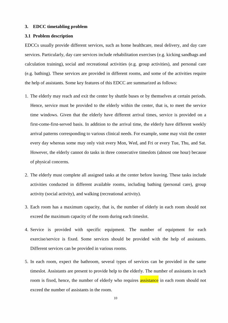
EDCCs usually provide different services, such as home healthcare, meal delivery, and day care

services. Particularly, day care services include rehabilitation exercises (e.g. kicking sandbags and

calculation training), social and recreational activities (e.g. group activities), and personal care

(e.g. bathing). These services are provided in different rooms, and some of the activities require

the help of assistants. Some key features of this EDCC are summarized as follows:

1. The elderly may reach and exit the center by shuttle buses or by themselves at certain periods.

Hence, service must be provided to the elderly within the center, that is, to meet the service

time windows. Given that the elderly have different arrival times, service is provided on a

first-come-first-served basis. In addition to the arrival time, the elderly have different weekly

arrival patterns corresponding to various clinical needs. For example, some may visit the center

every day whereas some may only visit every Mon, Wed, and Fri or every Tue, Thu, and Sat.

However, the elderly cannot do tasks in three consecutive timeslots (almost one hour) because

of physical concerns.

2. The elderly must complete all assigned tasks at the center before leaving. These tasks include

activities conducted in different available rooms, including bathing (personal care), group

activity (social activity), and walking (recreational activity).

3. Each room has a maximum capacity, that is, the number of elderly in each room should not

exceed the maximum capacity of the room during each timeslot.

4. Service is provided with specific equipment. The number of equipment for each

exercise/service is fixed. Some services should be provided with the help of assistants.

Different services can be provided in various rooms.

5. In each room, expect the bathroom, several types of services can be provided in the same

timeslot. Assistants are present to provide help to the elderly. The number of assistants in each

room is fixed, hence, the number of elderly who requires assistance in each room should not

exceed the number of assistants in the room.

11

6. Considering the health condition of the elderly, each timeslot is limited to 20 minutes, which is

shorter than those in the educational timetabling problem. The number of timeslots in each

working day can be calculated through the following equation: (end_time-start_time)/duration.

7. No restriction is imposed on the sequence of tasks for each elderly, that is, an activity can be

performed as long as the elderly and associated resources are available in the same timeslot.

The type and number of tasks for each elderly are designed based on his/her health condition

upon admission, but these tasks are subject to change after future evaluation.

8. Some group activities need to be performed only at fixed timeslots on certain days because of

some specific considerations, such as participant and room availabilities. An elderly who

participates in a group activity cannot perform other tasks during the same timeslot.

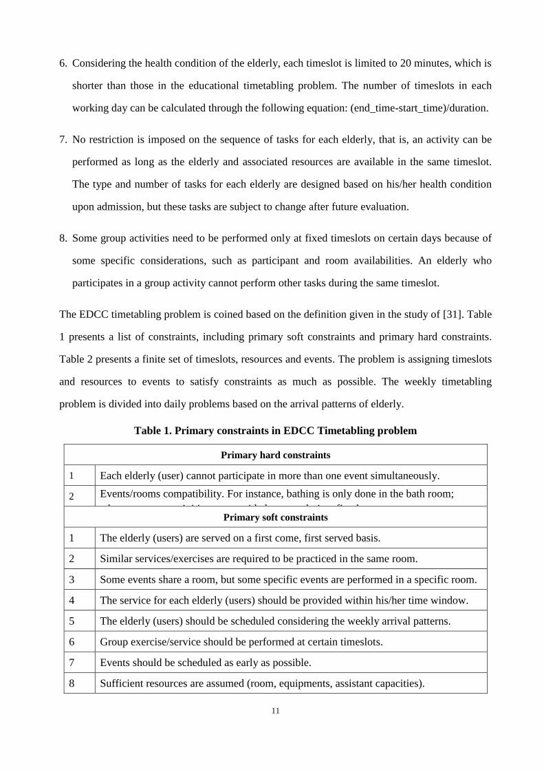
The EDCC timetabling problem is coined based on the definition given in the study of [31]. Table

1 presents a list of constraints, including primary soft constraints and primary hard constraints.

Table 2 presents a finite set of timeslots, resources and events. The problem is assigning timeslots

and resources to events to satisfy constraints as much as possible. The weekly timetabling

problem is divided into daily problems based on the arrival patterns of elderly.

Table 1. Primary constraints in EDCC Timetabling problem

Primary hard constraints

1 Each elderly (user) cannot participate in more than one event simultaneously.

2 Events/rooms compatibility. For instance, bathing is only done in the bath room;

whereas, group activities are provided separately in a fixed room. Primary soft constraints

1 The elderly (users) are served on a first come, first served basis.

2 Similar services/exercises are required to be practiced in the same room.

3 Some events share a room, but some specific events are performed in a specific room.

4 The service for each elderly (users) should be provided within his/her time window.

5 The elderly (users) should be scheduled considering the weekly arrival patterns.

6 Group exercise/service should be performed at certain timeslots.

7 Events should be scheduled as early as possible.

8 Sufficient resources are assumed (room, equipments, assistant capacities).

12

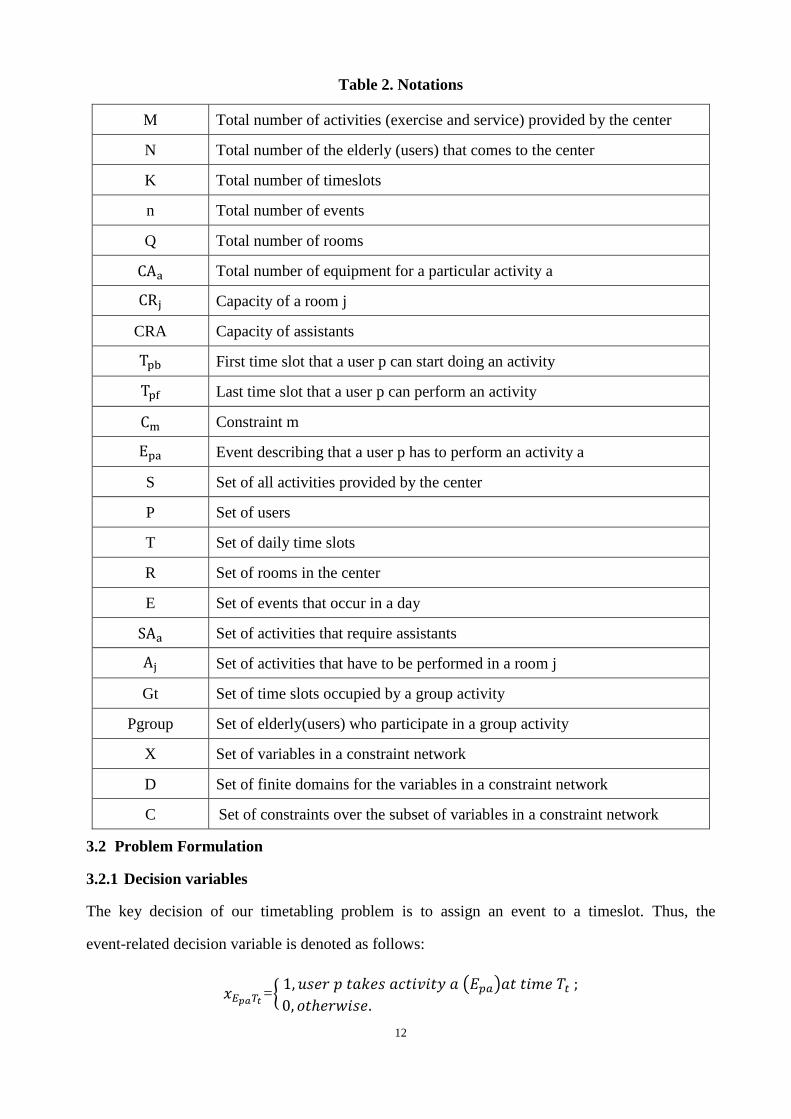
Table 2. Notations

M Total number of activities (exercise and service) provided by the center

N Total number of the elderly (users) that comes to the center

K Total number of timeslots

n Total number of events

Q Total number of rooms

CAa Total number of equipment for a particular activity a

CRj Capacity of a room j

CRA Capacity of assistants

Tpb First time slot that a user p can start doing an activity

Tpf Last time slot that a user p can perform an activity

Cm Constraint m

Epa Event describing that a user p has to perform an activity a

S Set of all activities provided by the center

P Set of users

T Set of daily time slots

R Set of rooms in the center

E Set of events that occur in a day

SAa Set of activities that require assistants

Aj Set of activities that have to be performed in a room j

Gt Set of time slots occupied by a group activity

Pgroup Set of elderly(users) who participate in a group activity

X Set of variables in a constraint network

D Set of finite domains for the variables in a constraint network

C Set of constraints over the subset of variables in a constraint network

3.2 Problem Formulation

3.2.1 Decision variables

The key decision of our timetabling problem is to assign an event to a timeslot. Thus, the

event-related decision variable is denoted as follows:

𝑥𝐸𝑝𝑎𝑇𝑡={

1, 𝑢𝑠𝑒𝑟 𝑝 𝑡𝑎𝑘𝑒𝑠 𝑎𝑐𝑡𝑖𝑣𝑖𝑡𝑦 𝑎 (𝐸𝑝𝑎)𝑎𝑡 𝑡𝑖𝑚𝑒 𝑇𝑡 ;

0, 𝑜𝑡ℎ𝑒𝑟𝑤𝑖𝑠𝑒.

13

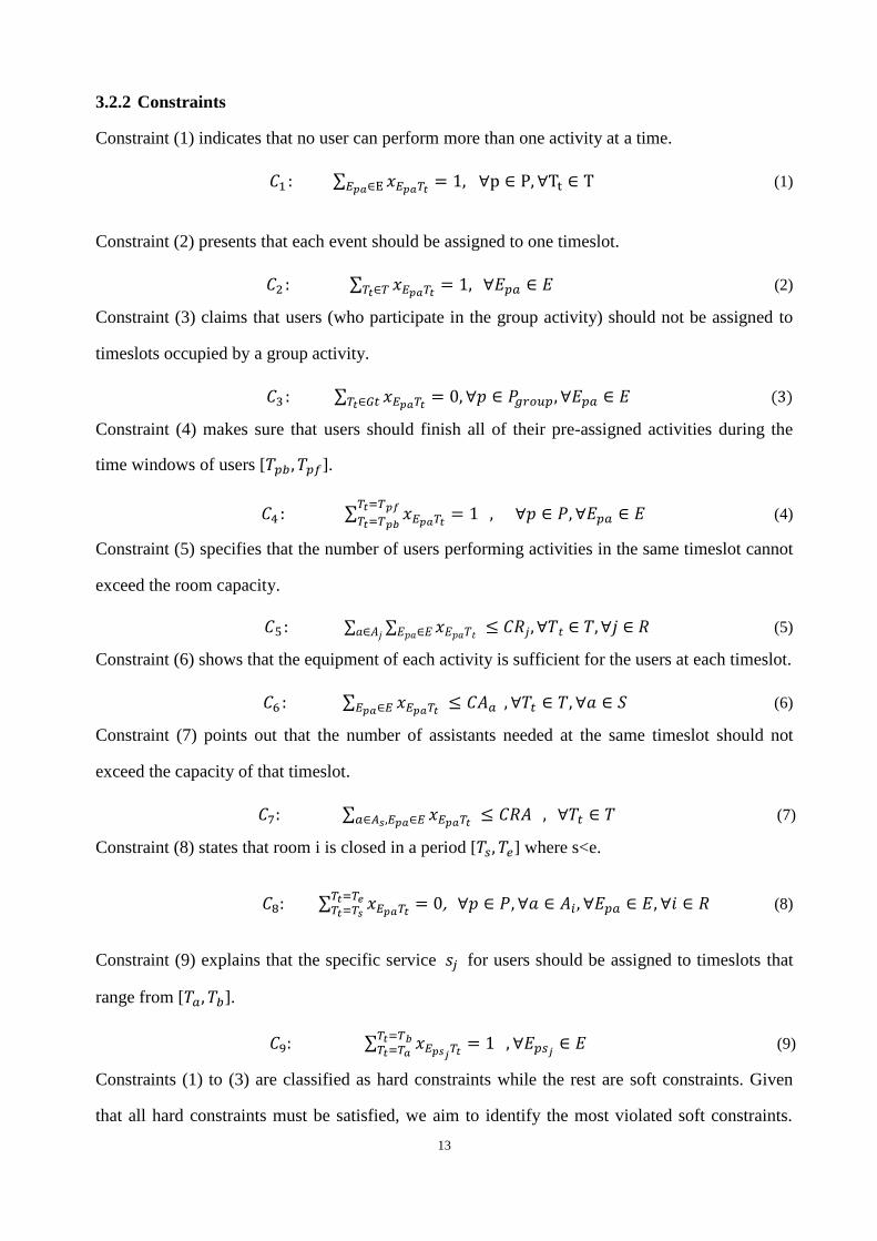
3.2.2 Constraints

Constraint (1) indicates that no user can perform more than one activity at a time.

𝐶1 : ∑ 𝑥𝐸𝑝𝑎𝑇𝑡𝐸𝑝𝑎∈E = 1, ∀p ∈ P, ∀Tt ∈ T (1)

Constraint (2) presents that each event should be assigned to one timeslot.

𝐶2 : ∑ 𝑥𝐸𝑝𝑎𝑇𝑡𝑇𝑡∈𝑇 = 1, ∀𝐸𝑝𝑎 ∈ 𝐸 (2)

Constraint (3) claims that users (who participate in the group activity) should not be assigned to

timeslots occupied by a group activity.

𝐶3 : ∑ 𝑥𝐸𝑝𝑎𝑇𝑡𝑇𝑡∈𝐺𝑡 = 0, ∀𝑝 ∈ 𝑃𝑔𝑟𝑜𝑢𝑝, ∀𝐸𝑝𝑎 ∈ 𝐸 (3)

Constraint (4) makes sure that users should finish all of their pre-assigned activities during the

time windows of users [𝑇𝑝𝑏 , 𝑇𝑝𝑓].

𝐶4 : ∑ 𝑥𝐸𝑝𝑎𝑇𝑡= 1

𝑇𝑡=𝑇𝑝𝑓

𝑇𝑡=𝑇𝑝𝑏 , ∀𝑝 ∈ 𝑃, ∀𝐸𝑝𝑎 ∈ 𝐸 (4)

Constraint (5) specifies that the number of users performing activities in the same timeslot cannot

exceed the room capacity.

𝐶5 : ∑ ∑ 𝑥𝐸𝑝𝑎𝑇𝑡𝐸𝑝𝑎∈𝐸𝑎∈𝐴𝑗 ≤ 𝐶𝑅𝑗, ∀𝑇𝑡 ∈ 𝑇, ∀𝑗 ∈ 𝑅 (5)

Constraint (6) shows that the equipment of each activity is sufficient for the users at each timeslot.

𝐶6 : ∑ 𝑥𝐸𝑝𝑎𝑇𝑡 ≤ 𝐶𝐴𝑎𝐸𝑝𝑎∈𝐸 , ∀𝑇𝑡 ∈ 𝑇, ∀𝑎 ∈ 𝑆 (6)

Constraint (7) points out that the number of assistants needed at the same timeslot should not

exceed the capacity of that timeslot.

𝐶7: ∑ 𝑥𝐸𝑝𝑎𝑇𝑡 ≤ 𝐶𝑅𝐴𝑎∈𝐴𝑠,𝐸𝑝𝑎∈𝐸 , ∀𝑇𝑡 ∈ 𝑇 (7)

Constraint (8) states that room i is closed in a period [𝑇𝑠, 𝑇𝑒] where s<e.

𝐶8: ∑ 𝑥𝐸𝑝𝑎𝑇𝑡= 0

𝑇𝑡=𝑇𝑒𝑇𝑡=𝑇𝑠

, ∀𝑝 ∈ 𝑃, ∀𝑎 ∈ 𝐴𝑖, ∀𝐸𝑝𝑎 ∈ 𝐸, ∀𝑖 ∈ 𝑅 (8)

Constraint (9) explains that the specific service 𝑠𝑗 for users should be assigned to timeslots that

range from [𝑇𝑎, 𝑇𝑏].

𝐶9: ∑ 𝑥𝐸𝑝𝑠𝑗𝑇𝑡

= 1𝑇𝑡=𝑇𝑏𝑇𝑡=𝑇𝑎

, ∀𝐸𝑝𝑠𝑗∈ 𝐸 (9)

Constraints (1) to (3) are classified as hard constraints while the rest are soft constraints. Given

that all hard constraints must be satisfied, we aim to identify the most violated soft constraints.

14

These soft constraints may indicate the potential improvement for an EDCC if some of the

constraints can be relaxed, for example, increasing the room capacity and the number of

equipment, and extending the opening hours.

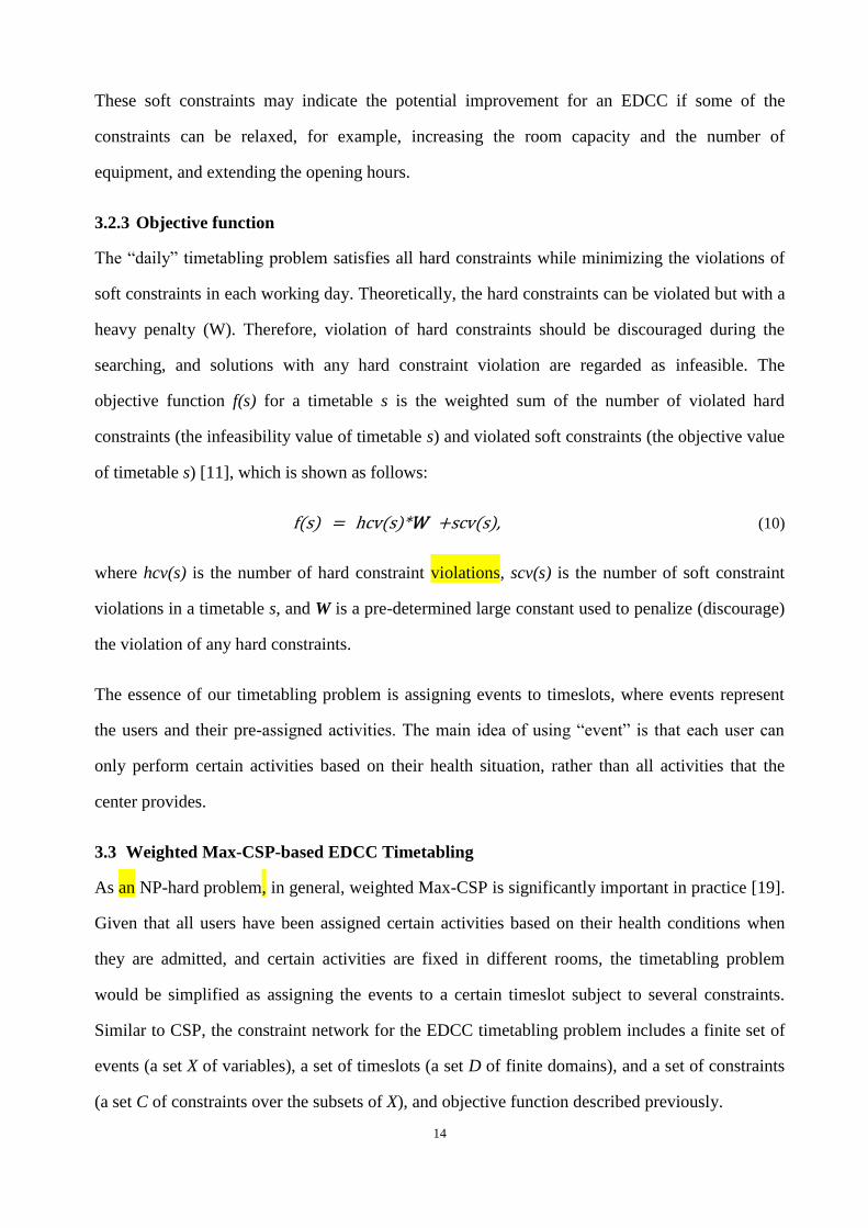
3.2.3 Objective function

The “daily” timetabling problem satisfies all hard constraints while minimizing the violations of

soft constraints in each working day. Theoretically, the hard constraints can be violated but with a

heavy penalty (W). Therefore, violation of hard constraints should be discouraged during the

searching, and solutions with any hard constraint violation are regarded as infeasible. The

objective function f(s) for a timetable s is the weighted sum of the number of violated hard

constraints (the infeasibility value of timetable s) and violated soft constraints (the objective value

of timetable s) [11], which is shown as follows:

f(s) = hcv(s)*W +scv(s), (10)

where hcv(s) is the number of hard constraint violations, scv(s) is the number of soft constraint

violations in a timetable s, and W is a pre-determined large constant used to penalize (discourage)

the violation of any hard constraints.

The essence of our timetabling problem is assigning events to timeslots, where events represent

the users and their pre-assigned activities. The main idea of using “event” is that each user can

only perform certain activities based on their health situation, rather than all activities that the

center provides.

3.3 Weighted Max-CSP-based EDCC Timetabling

As an NP-hard problem, in general, weighted Max-CSP is significantly important in practice [19].

Given that all users have been assigned certain activities based on their health conditions when

they are admitted, and certain activities are fixed in different rooms, the timetabling problem

would be simplified as assigning the events to a certain timeslot subject to several constraints.

Similar to CSP, the constraint network for the EDCC timetabling problem includes a finite set of

events (a set X of variables), a set of timeslots (a set D of finite domains), and a set of constraints

(a set C of constraints over the subsets of X), and objective function described previously.

15

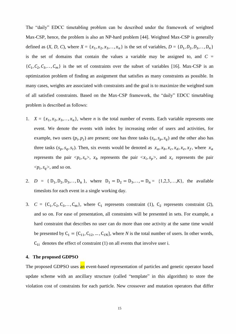
The “daily” EDCC timetabling problem can be described under the framework of weighted

Max-CSP, hence, the problem is also an NP-hard problem [44]. Weighted Max-CSP is generally

defined as (X, D, C), where X = {𝑥1, 𝑥2, 𝑥3, . . , 𝑥𝑛} is the set of variables, D = {𝐷1, 𝐷2, 𝐷3, . . , 𝐷𝑛}

is the set of domains that contain the values a variable may be assigned to, and C =

{𝐶1, 𝐶2, 𝐶3, . . , 𝐶𝑚} is the set of constraints over the subset of variables [16]. Max-CSP is an

optimization problem of finding an assignment that satisfies as many constraints as possible. In

many cases, weights are associated with constraints and the goal is to maximize the weighted sum

of all satisfied constraints. Based on the Max-CSP framework, the “daily” EDCC timetabling

problem is described as follows:

1. X = {𝑥1, 𝑥2, 𝑥3, . . , 𝑥𝑛}, where n is the total number of events. Each variable represents one

event. We denote the events with index by increasing order of users and activities, for

example, two users (𝑝𝑖, 𝑝𝑗) are present; one has three tasks (𝑠𝑜 , 𝑠𝑝, 𝑠𝑞) and the other also has

three tasks (𝑠𝑝, 𝑠𝑞 , 𝑠𝑡). Then, six events would be denoted as 𝑥𝑎, 𝑥𝑏 , 𝑥𝑐, 𝑥𝑑, 𝑥𝑒 , 𝑥𝑓, where 𝑥𝑎

represents the pair <𝑝𝑖 , 𝑠𝑜>, 𝑥𝑏 represents the pair <𝑥𝑖 , 𝑠𝑝>, and 𝑥𝑐 represents the pair

<𝑝𝑖, 𝑠𝑞>, and so on.

2. D = { D1, D2, D3, . . , Dn }, where D1 = D2 = D3, . . , = Dn = {1,2,3,…,K}, the available

timeslots for each event in a single working day.

3. C = {C1, C2, C3, . . , Cm}, where C1 represents constraint (1), C2 represents constraint (2),

and so on. For ease of presentation, all constraints will be presented in sets. For example, a

hard constraint that describes no user can do more than one activity at the same time would

be presented by C1 = {C11, C12, … , C1N}, where N is the total number of users. In other words,

C1i denotes the effect of constraint (1) on all events that involve user i.

4. The proposed GDPSO

The proposed GDPSO uses an event-based representation of particles and genetic operator based

update scheme with an ancillary structure (called “template” in this algorithm) to store the

violation cost of constraints for each particle. New crossover and mutation operators that differ

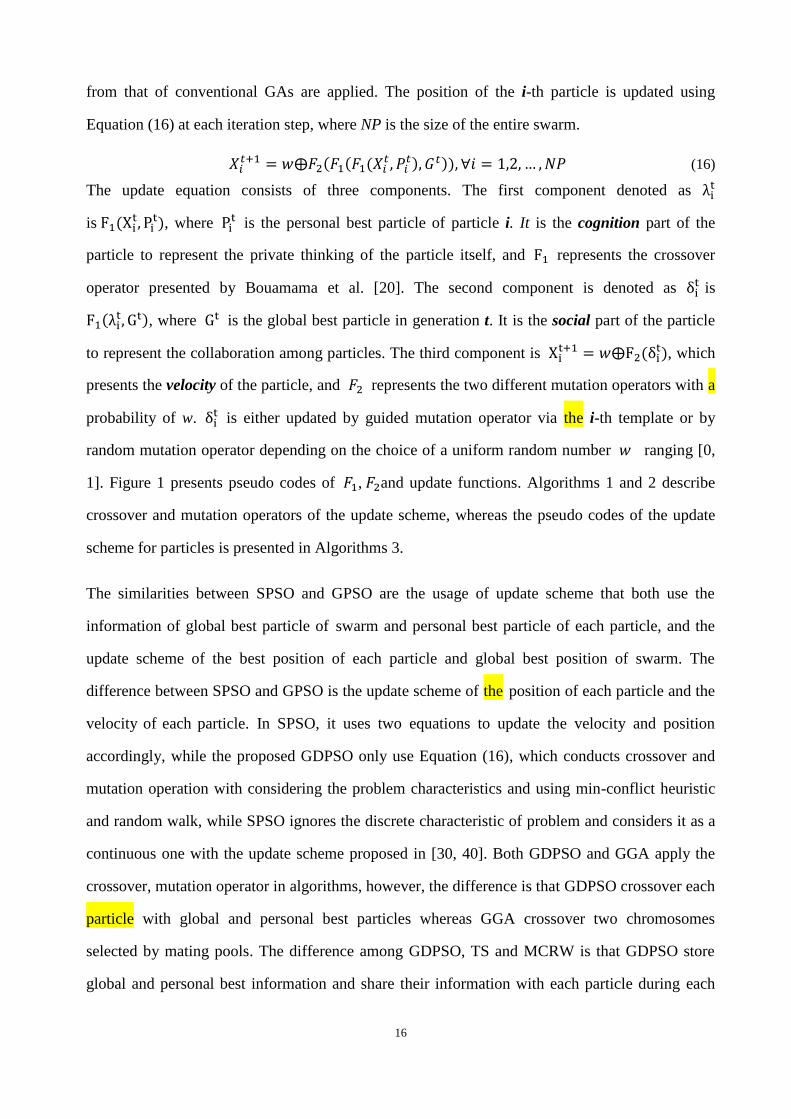
16

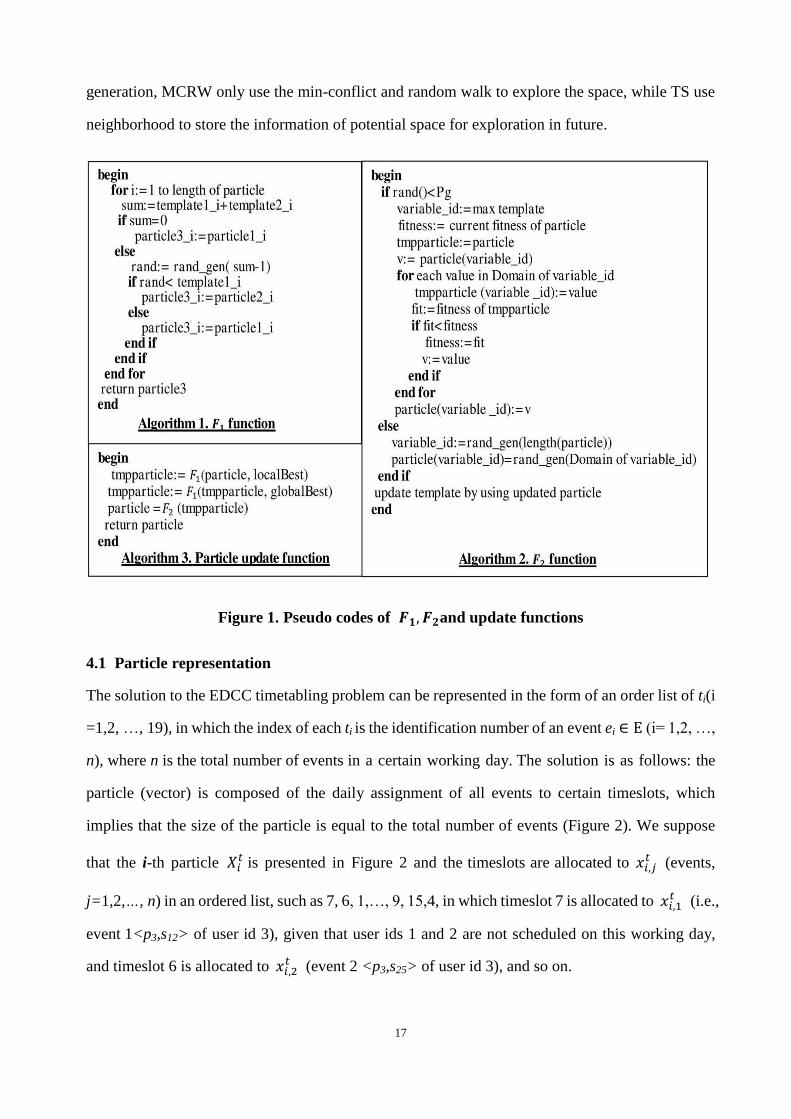
from that of conventional GAs are applied. The position of the i-th particle is updated using

Equation (16) at each iteration step, where NP is the size of the entire swarm.

𝑋𝑖𝑡+1 = 𝑤⨁𝐹2(𝐹1(𝐹1(𝑋𝑖

𝑡 , 𝑃𝑖𝑡), 𝐺𝑡)), ∀𝑖 = 1,2, … , 𝑁𝑃 (16)

The update equation consists of three components. The first component denoted as λit

is F1(Xit, Pi

t), where Pit is the personal best particle of particle i. It is the cognition part of the

particle to represent the private thinking of the particle itself, and F1 represents the crossover

operator presented by Bouamama et al. [20]. The second component is denoted as δit is

F1(λit, Gt), where Gt is the global best particle in generation t. It is the social part of the particle

to represent the collaboration among particles. The third component is Xit+1 = 𝑤⨁F2(δi

t), which

presents the velocity of the particle, and 𝐹2 represents the two different mutation operators with a

probability of w. δit is either updated by guided mutation operator via the i-th template or by

random mutation operator depending on the choice of a uniform random number 𝑤 ranging [0,

1]. Figure 1 presents pseudo codes of 𝐹1, 𝐹2and update functions. Algorithms 1 and 2 describe

crossover and mutation operators of the update scheme, whereas the pseudo codes of the update

scheme for particles is presented in Algorithms 3.

The similarities between SPSO and GPSO are the usage of update scheme that both use the

information of global best particle of swarm and personal best particle of each particle, and the

update scheme of the best position of each particle and global best position of swarm. The

difference between SPSO and GPSO is the update scheme of the position of each particle and the

velocity of each particle. In SPSO, it uses two equations to update the velocity and position

accordingly, while the proposed GDPSO only use Equation (16), which conducts crossover and

mutation operation with considering the problem characteristics and using min-conflict heuristic

and random walk, while SPSO ignores the discrete characteristic of problem and considers it as a

continuous one with the update scheme proposed in [30, 40]. Both GDPSO and GGA apply the

crossover, mutation operator in algorithms, however, the difference is that GDPSO crossover each

particle with global and personal best particles whereas GGA crossover two chromosomes

selected by mating pools. The difference among GDPSO, TS and MCRW is that GDPSO store

global and personal best information and share their information with each particle during each

17

generation, MCRW only use the min-conflict and random walk to explore the space, while TS use

neighborhood to store the information of potential space for exploration in future.

Figure 1. Pseudo codes of 𝑭𝟏, 𝑭𝟐and update functions

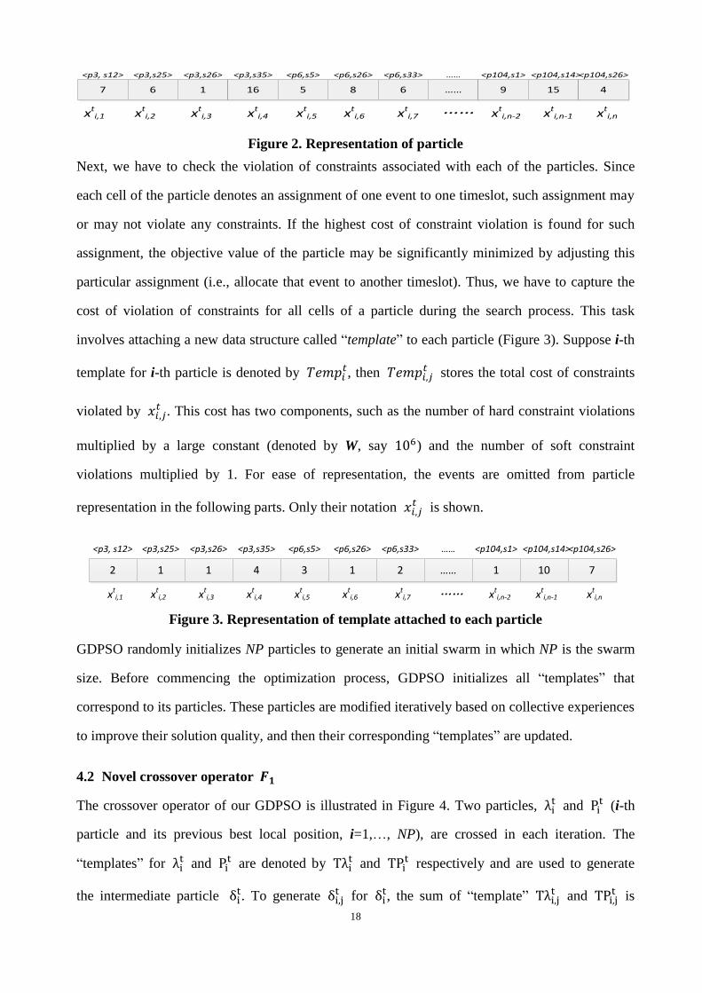
4.1 Particle representation

The solution to the EDCC timetabling problem can be represented in the form of an order list of ti(i

=1,2, …, 19), in which the index of each ti is the identification number of an event ei ∈ E (i= 1,2, …,

n), where n is the total number of events in a certain working day. The solution is as follows: the

particle (vector) is composed of the daily assignment of all events to certain timeslots, which

implies that the size of the particle is equal to the total number of events (Figure 2). We suppose

that the i-th particle 𝑋𝑖𝑡 is presented in Figure 2 and the timeslots are allocated to 𝑥𝑖,𝑗

𝑡 (events,

j=1,2,…, n) in an ordered list, such as 7, 6, 1,…, 9, 15,4, in which timeslot 7 is allocated to 𝑥𝑖,1𝑡 (i.e.,

event 1<p3,s12> of user id 3), given that user ids 1 and 2 are not scheduled on this working day,

and timeslot 6 is allocated to 𝑥𝑖,2𝑡 (event 2 <p3,s25> of user id 3), and so on.

18

7 6 1 16 5 8 6 …… 9 15 4

<p3, s12> <p3,s25> <p3,s26> <p3,s35> <p6,s5> <p6,s26> <p6,s33> …… <p104,s1> <p104,s14><p104,s26>

xti,1 xt

i,2 xti,3 xt

i,4 xti,5 xt

i,6 xti,7 xt

i,n-2 xti,n-1 xt

i,n……

Figure 2. Representation of particle

Next, we have to check the violation of constraints associated with each of the particles. Since

each cell of the particle denotes an assignment of one event to one timeslot, such assignment may

or may not violate any constraints. If the highest cost of constraint violation is found for such

assignment, the objective value of the particle may be significantly minimized by adjusting this

particular assignment (i.e., allocate that event to another timeslot). Thus, we have to capture the

cost of violation of constraints for all cells of a particle during the search process. This task

involves attaching a new data structure called “template” to each particle (Figure 3). Suppose i-th

template for i-th particle is denoted by 𝑇𝑒𝑚𝑝𝑖𝑡, then 𝑇𝑒𝑚𝑝𝑖,𝑗

𝑡 stores the total cost of constraints

violated by 𝑥𝑖,𝑗𝑡 . This cost has two components, such as the number of hard constraint violations

multiplied by a large constant (denoted by W, say 106) and the number of soft constraint

violations multiplied by 1. For ease of representation, the events are omitted from particle

representation in the following parts. Only their notation 𝑥𝑖,𝑗𝑡 is shown.

2 1 1 4 3 1 2 …… 1 10 7

<p3, s12> <p3,s25> <p3,s26> <p3,s35> <p6,s5> <p6,s26> <p6,s33> …… <p104,s1> <p104,s14><p104,s26>

xti,1 xt

i,2 xti,3 xt

i,4 xti,5 xt

i,6 xti,7 xt

i,n-2 xti,n-1 xt

i,n……

Figure 3. Representation of template attached to each particle

GDPSO randomly initializes NP particles to generate an initial swarm in which NP is the swarm

size. Before commencing the optimization process, GDPSO initializes all “templates” that

correspond to its particles. These particles are modified iteratively based on collective experiences

to improve their solution quality, and then their corresponding “templates” are updated.

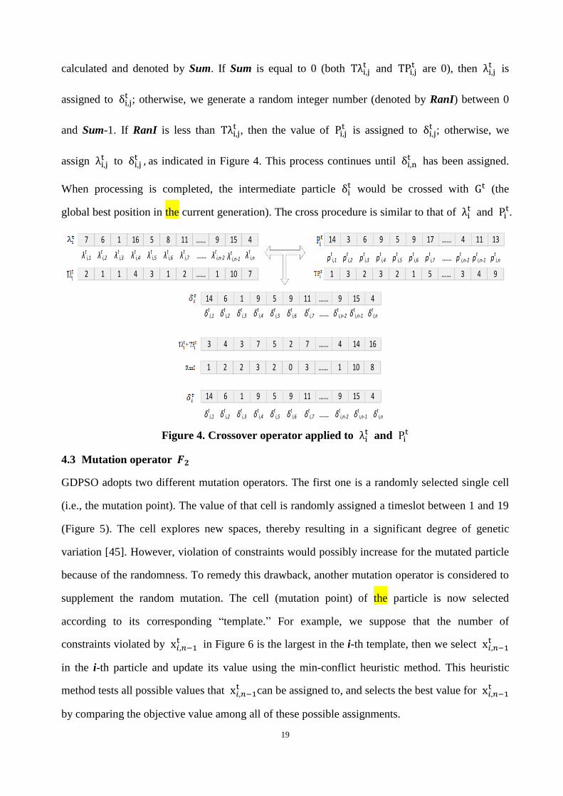
4.2 Novel crossover operator 𝑭𝟏

The crossover operator of our GDPSO is illustrated in Figure 4. Two particles, λit and Pi

t (i-th

particle and its previous best local position, i=1,…, NP), are crossed in each iteration. The

“templates” for λit and Pi

t are denoted by Tλit and TPi

t respectively and are used to generate

the intermediate particle δit. To generate δi,j

t for δit, the sum of “template” Tλi,j

t and TPi,jt is

19

calculated and denoted by Sum. If Sum is equal to 0 (both Tλi,jt and TPi,j

t are 0), then λi,jt is

assigned to δi,jt ; otherwise, we generate a random integer number (denoted by RanI) between 0

and Sum-1. If RanI is less than Tλi,jt , then the value of Pi,j

t is assigned to δi,jt ; otherwise, we

assign λi,jt to δi,j

t , as indicated in Figure 4. This process continues until δi,nt has been assigned.

When processing is completed, the intermediate particle δit would be crossed with Gt (the

global best position in the current generation). The cross procedure is similar to that of λit and Pi

t.

7 6 1 16 5 8 11 …… 9 15 4

λti,1 λt

i,2 λti,3 λt

i,4 λti,5 λt

i,6 λti,7 λt

i,n-2 λti,n-1 λt

i,n……

2 1 1 4 3 1 2 …… 1 10 7 1 3 2 3 2 1 5 …… 3 4 9

14 3 6 9 5 9 17 …… 4 11 13

14 6 1 9 5 9 11 …… 9 15 4

3 4 3 7 5 2 7 …… 4 14 16

1 2 2 3 2 0 3 …… 1 10 8

14 6 1 9 5 9 11 …… 9 15 4

pti,1 pt

i,2 pti,3 pt

i,4 pti,5 pt

i,6 pti,7 pt

i,n-2 pti,n-1 pt

i,n……

δti,1 δt

i,2 δti,3 δt

i,4 δti,5 δt

i,6 δti,7 δt

i,n-2 δti,n-1 δt

i,n……

δti,1 δt

i,2 δti,3 δt

i,4 δti,5 δt

i,6 δti,7 δt

i,n-2 δti,n-1 δt

i,n……

Figure 4. Crossover operator applied to λit and Pi

t

4.3 Mutation operator 𝑭𝟐

GDPSO adopts two different mutation operators. The first one is a randomly selected single cell

(i.e., the mutation point). The value of that cell is randomly assigned a timeslot between 1 and 19

(Figure 5). The cell explores new spaces, thereby resulting in a significant degree of genetic

variation [45]. However, violation of constraints would possibly increase for the mutated particle

because of the randomness. To remedy this drawback, another mutation operator is considered to

supplement the random mutation. The cell (mutation point) of the particle is now selected

according to its corresponding “template.” For example, we suppose that the number of

constraints violated by x𝑖,𝑛−1t in Figure 6 is the largest in the i-th template, then we select x𝑖,𝑛−1

t

in the i-th particle and update its value using the min-conflict heuristic method. This heuristic

method tests all possible values that x𝑖,𝑛−1t can be assigned to, and selects the best value for x𝑖,𝑛−1

t

by comparing the objective value among all of these possible assignments.

20

7 6 1 16 5 8 11 …… 9 15 4

xti,1 xt

i,2 xti,3 xt

i,4 xti,5 xt

i,6 xti,7 xt

i,n-2 xti,n-1 xt

i,n……

particle

7 6 1 16 5 2 11 …… 9 6 4

xti,1 xt

i,2 xti,3 xt

i,4 xti,5 xt

i,6 xti,7 xt

i,n-2 xti,n-1 xt

i,n……

particle 15

Figure 5.Mutation operator with random selected j for 𝑋𝑖𝑡

7 6 1 16 5 8 11 …… 9 15 4

xti,1 xt

i,2 xti,3 xt

i,4 xti,5 xt

i,6 xti,7 xt

i,n-2 xti,n-1 xt

i,n……

2 1 1 4 3 1 2 …… 1 10 7

particle

template

7 6 1 16 5 8 11 …… 9 6 4

xti,1 xt

i,2 xti,3 xt

i,4 xti,5 xt

i,6 xti,7 xt

i,n-2 xti,n-1 xt

i,n……

1 2 1 2 5 2 7 …… 2 11 2

particle

template

Figure 6.Mutation operator with min-conflict heuristic

4.4 Fitness evaluation

As defined by Equation (10), the objective is to minimize the violation of hard and as many soft

constraints as possible. The fitness evaluation uses the objective function to calculate the fitness

of each particle, which implies that smaller fitness (smaller constraint violation cost) of a particle

results in a better solution.

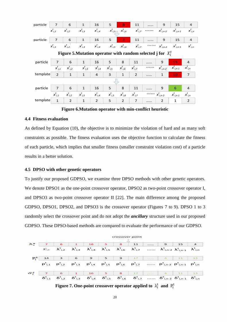
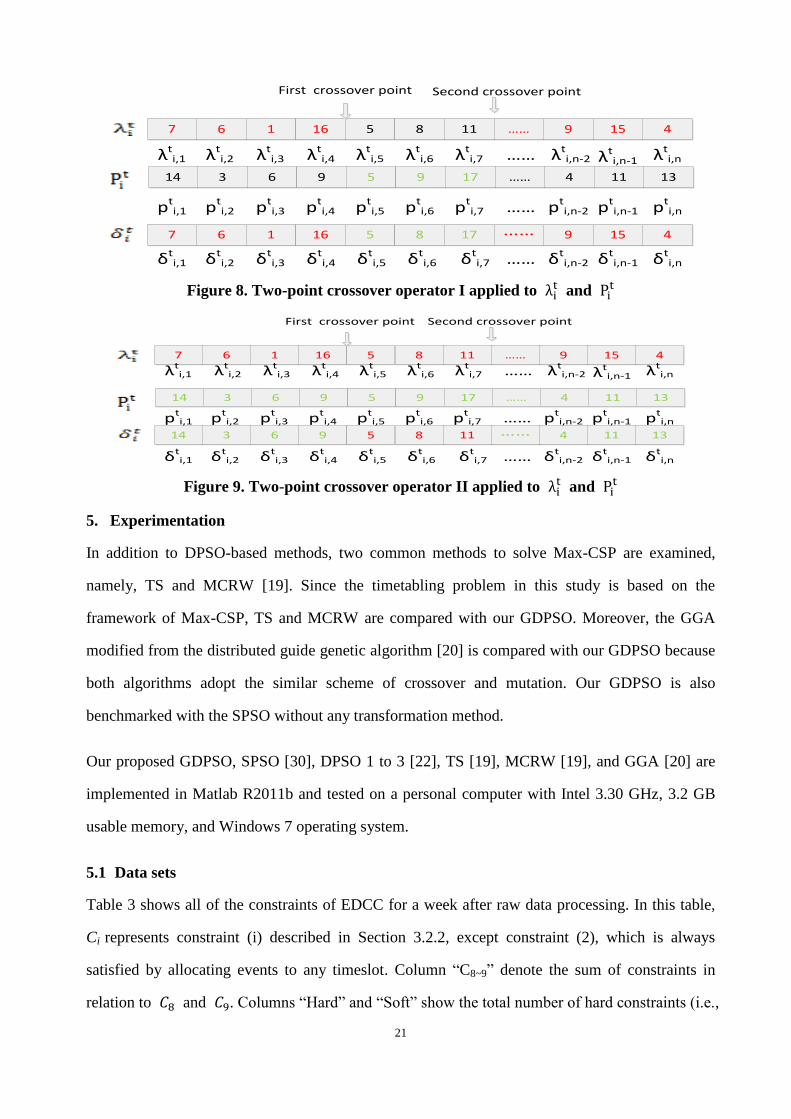
4.5 DPSO with other genetic operators

To justify our proposed GDPSO, we examine three DPSO methods with other genetic operators.

We denote DPSO1 as the one-point crossover operator, DPSO2 as two-point crossover operator I,

and DPSO3 as two-point crossover operator II [22]. The main difference among the proposed

GDPSO, DPSO1, DPSO2, and DPSO3 is the crossover operator (Figures 7 to 9). DPSO 1 to 3

randomly select the crossover point and do not adopt the ancillary structure used in our proposed

GDPSO. These DPSO-based methods are compared to evaluate the performance of our GDPSO.

7 6 1 16 5 8 11 …… 9 15 4

λti,1 λt

i,2 λti,3 λt

i,4 λti,5 λt

i,6 λti,7 λt

i,n-2 λti,n-1 λt

i,n……

14 3 6 9 5 9 17 …… 4 11 13

pti,1 pt

i,2 pti,3 pt

i,4 pti,5 pt

i,6 pti,7 pt

i,n-2 pti,n-1 pt

i,n……

7 6 1 16 5 8 17 …… 4 11 13

δti,1 δt

i,2 δti,3 δt

i,4 δti,5 δt

i,6 δti,7 δt

i,n-2 δti,n-1 δt

i,n……

crossover point

Figure 7. One-point crossover operator applied to λit and Pi

t

21

7 6 1 16 5 8 11 …… 9 15 4

λti,1 λt

i,2 λti,3 λt

i,4 λti,5 λt

i,6 λti,7 λt

i,n-2 λti,n-1 λt

i,n……

First crossover point Second crossover point

14 3 6 9 5 9 17 …… 4 11 13

pti,1 pt

i,2 pti,3 pt

i,4 pti,5 pt

i,6 pti,7 pt

i,n-2 pti,n-1 pt

i,n……

7 6 1 16 5 8 17 …… 9 15 4

δti,1 δt

i,2 δti,3 δt

i,4 δti,5 δt

i,6 δti,7 δt

i,n-2 δti,n-1 δt

i,n……

Figure 8. Two-point crossover operator I applied to λit and Pi

t

7 6 1 16 5 8 11 …… 9 15 4

First crossover point Second crossover point

14 3 6 9 5 9 17 …… 4 11 13

14 3 6 9 5 8 11 …… 4 11 13

δti,1 δt

i,2 δti,3 δt

i,4 δti,5 δt

i,6 δti,7 δt

i,n-2 δti,n-1 δt

i,n……

pti,1 pt

i,2 pti,3 pt

i,4 pti,5 pt

i,6 pti,7 pt

i,n-2 pti,n-1 pt

i,n……

λti,1 λt

i,2 λti,3 λt

i,4 λti,5 λt

i,6 λti,7 λt

i,n-2 λti,n-1 λt

i,n……

Figure 9. Two-point crossover operator II applied to λit and Pi

t

5. Experimentation

In addition to DPSO-based methods, two common methods to solve Max-CSP are examined,

namely, TS and MCRW [19]. Since the timetabling problem in this study is based on the

framework of Max-CSP, TS and MCRW are compared with our GDPSO. Moreover, the GGA

modified from the distributed guide genetic algorithm [20] is compared with our GDPSO because

both algorithms adopt the similar scheme of crossover and mutation. Our GDPSO is also

benchmarked with the SPSO without any transformation method.

Our proposed GDPSO, SPSO [30], DPSO 1 to 3 [22], TS [19], MCRW [19], and GGA [20] are

implemented in Matlab R2011b and tested on a personal computer with Intel 3.30 GHz, 3.2 GB

usable memory, and Windows 7 operating system.

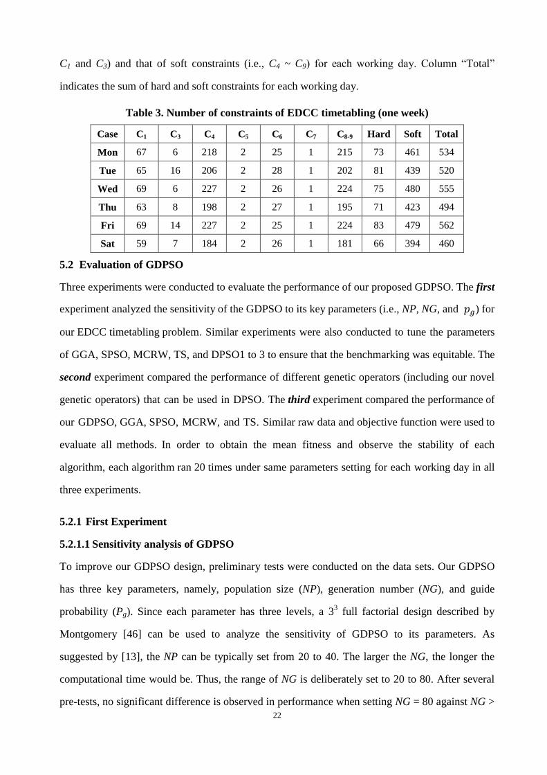
5.1 Data sets

Table 3 shows all of the constraints of EDCC for a week after raw data processing. In this table,

Ci represents constraint (i) described in Section 3.2.2, except constraint (2), which is always

satisfied by allocating events to any timeslot. Column “C8~9” denote the sum of constraints in

relation to 𝐶8 and 𝐶9. Columns “Hard” and “Soft” show the total number of hard constraints (i.e.,

22

C1 and C3) and that of soft constraints (i.e., C4 ~ C9) for each working day. Column “Total”

indicates the sum of hard and soft constraints for each working day.

Table 3. Number of constraints of EDCC timetabling (one week)

Case C1 C3 C4 C5 C6 C7 C8-9 Hard Soft Total

Mon 67 6 218 2 25 1 215 73 461 534

Tue 65 16 206 2 28 1 202 81 439 520

Wed 69 6 227 2 26 1 224 75 480 555

Thu 63 8 198 2 27 1 195 71 423 494

Fri 69 14 227 2 25 1 224 83 479 562

Sat 59 7 184 2 26 1 181 66 394 460

5.2 Evaluation of GDPSO

Three experiments were conducted to evaluate the performance of our proposed GDPSO. The first

experiment analyzed the sensitivity of the GDPSO to its key parameters (i.e., NP, NG, and 𝑝𝑔) for

our EDCC timetabling problem. Similar experiments were also conducted to tune the parameters

of GGA, SPSO, MCRW, TS, and DPSO1 to 3 to ensure that the benchmarking was equitable. The

second experiment compared the performance of different genetic operators (including our novel

genetic operators) that can be used in DPSO. The third experiment compared the performance of

our GDPSO, GGA, SPSO, MCRW, and TS. Similar raw data and objective function were used to

evaluate all methods. In order to obtain the mean fitness and observe the stability of each

algorithm, each algorithm ran 20 times under same parameters setting for each working day in all

three experiments.

5.2.1 First Experiment

5.2.1.1 Sensitivity analysis of GDPSO

To improve our GDPSO design, preliminary tests were conducted on the data sets. Our GDPSO

has three key parameters, namely, population size (NP), generation number (NG), and guide

probability (Pg). Since each parameter has three levels, a 33 full factorial design described by

Montgomery [46] can be used to analyze the sensitivity of GDPSO to its parameters. As

suggested by [13], the NP can be typically set from 20 to 40. The larger the NG, the longer the

computational time would be. Thus, the range of NG is deliberately set to 20 to 80. After several

pre-tests, no significant difference is observed in performance when setting NG = 80 against NG >

23

80. The range of Pg is set to 0.3 to 0.8 because this parameter requires longer computing time

when Pg = 1. The performance (Pg = 1) is insignificantly different from that of Pg = 0.8, but the

performance (Pg = 0.3) is significantly different from that of Pg = 0. Experimentally, three levels

of each parameter {low, medium, high} are set as: NP {20, 30, 40}, NG {20, 40, 80}, and Pg {0.3,

0.5, 0.8}.

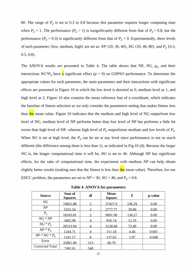
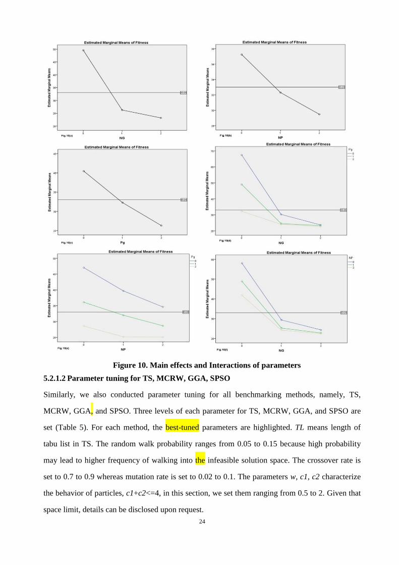
The ANOVA results are presented in Table 4. The table shows that NP, NG, pg, and their

interactions NG*Pg have a significant effect (p = 0) on GDPSO performance. To determine the

appropriate values for each parameter, the main parameters and their interactions with significant

effects are presented in Figure 10 in which the low level is denoted as 0, medium level as 1, and

high level as 2. Figure 10 also contains the mean reference line of y-coordinate, which indicates

the baseline of fitness selection so we only consider the parameters setting that makes fitness less

than the mean value. Figure 10 indicates that the medium and high level of NG outperform low

level of NG, medium level of NP performs better than low level of NP but performs a little bit

worse than high level of NP, whereas high level of Pg outperforms medium and low levels of Pg.

When NG is set at high level, the Pg can be set at any level since performance is not so much

different (the difference among them is less than 1), as indicated in Fig.10 (d). Because the larger

NG is, the longer computational time it will be, NG is set to 40. Although NP has significant

effects, for the sake of computational time, the experiment with medium NP can help obtain

slightly better results (making sure that the fitness is less than the mean value). Therefore, for our

EDCC problem, the parameters are set to NP = 30, NG = 40, and Pg = 0.8.

Table 4. ANOVA for parameters

Source Sum of

Squares df

Mean

Square F p-value

NG 74855.88 2 37427.9 536.29 0.00

NP 5555.54 2 2777.77 39.80 0.00

Pg 18183.81 2 9091.90 130.27 0.00 NG * NP

3402.98 4 850.74 12.19 0.00 NG * Pg 20513.94 4 5128.48 73.49 0.00 NP * Pg 1244.71 4 311.18 4.46 0.001

NP * NG * Pg 1101.17 8 137.65 1.97 0.048 Error

35801.90 513 69.79 Corrected Total

749116 540

24

Figure 10. Main effects and Interactions of parameters

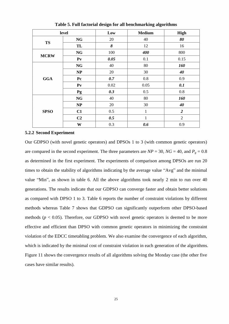
5.2.1.2 Parameter tuning for TS, MCRW, GGA, SPSO

Similarly, we also conducted parameter tuning for all benchmarking methods, namely, TS,

MCRW, GGA, and SPSO. Three levels of each parameter for TS, MCRW, GGA, and SPSO are

set (Table 5). For each method, the best-tuned parameters are highlighted. TL means length of

tabu list in TS. The random walk probability ranges from 0.05 to 0.15 because high probability

may lead to higher frequency of walking into the infeasible solution space. The crossover rate is

set to 0.7 to 0.9 whereas mutation rate is set to 0.02 to 0.1. The parameters w, c1, c2 characterize

the behavior of particles, c1+c2<=4, in this section, we set them ranging from 0.5 to 2. Given that

space limit, details can be disclosed upon request.

25

Table 5. Full factorial design for all benchmarking algorithms

level Low Medium High

TS NG 20 40 80

TL 8 12 16

MCRW NG 100 400 800

Pv 0.05 0.1 0.15

GGA

NG 40 80 160

NP 20 30 40

Pc 0.7 0.8 0.9

Pv 0.02 0.05 0.1

Pg 0.3 0.5 0.8

SPSO

NG 40 80 160

NP 20 30 40

C1 0.5 1 2

C2 0.5 1 2

W 0.3 0.6 0.9

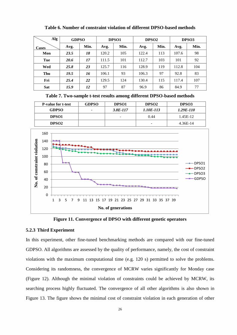
5.2.2 Second Experiment

Our GDPSO (with novel genetic operators) and DPSOs 1 to 3 (with common genetic operators)

are compared in the second experiment. The three parameters are NP = 30, NG = 40, and Pg = 0.8

as determined in the first experiment. The experiments of comparison among DPSOs are run 20

times to obtain the stability of algorithms indicating by the average value “Avg” and the minimal

value “Min”, as shown in table 6. All the above algorithms took nearly 2 min to run over 40

generations. The results indicate that our GDPSO can converge faster and obtain better solutions

as compared with DPSO 1 to 3. Table 6 reports the number of constraint violations by different

methods whereas Table 7 shows that GDPSO can significantly outperform other DPSO-based

methods (p < 0.05). Therefore, our GDPSO with novel genetic operators is deemed to be more

effective and efficient than DPSO with common genetic operators in minimizing the constraint

violation of the EDCC timetabling problem. We also examine the convergence of each algorithm,

which is indicated by the minimal cost of constraint violation in each generation of the algorithms.

Figure 11 shows the convergence results of all algorithms solving the Monday case (the other five

cases have similar results).

26

Table 6. Number of constraint violation of different DPSO-based methods

Alg

Cases

GDPSO DPSO1 DPSO2 DPSO3

Avg. Min. Avg. Min. Avg. Min. Avg. Min.

Mon 23.5 18 120.2 105 122.4 113 107.6 98

Tue 20.6 17 111.5 101 112.7 103 101 92

Wed 25.8 23 125.7 116 128.9 119 112.8 104

Thu 19.5 16 106.1 93 106.3 97 92.8 83

Fri 25.4 22 129.5 124 130.4 115 117.4 107

Sat 15.9 12 97 87 96.9 86 84.9 77

Table 7. Two-sample t-test results among different DPSO-based methods

P-value for t-test GDPSO DPSO1 DPSO2 DPSO3

GDPSO - 3.8E-117 1.10E-113 1.29E-110

DPSO1 - 0.44 1.45E-12

DPSO2 - 4.36E-14

Figure 11. Convergence of DPSO with different genetic operators

5.2.3 Third Experiment

In this experiment, other fine-tuned benchmarking methods are compared with our fine-tuned

GDPSO. All algorithms are assessed by the quality of performance, namely, the cost of constraint

violations with the maximum computational time (e.g. 120 s) permitted to solve the problems.

Considering its randomness, the convergence of MCRW varies significantly for Monday case

(Figure 12). Although the minimal violation of constraints could be achieved by MCRW, its

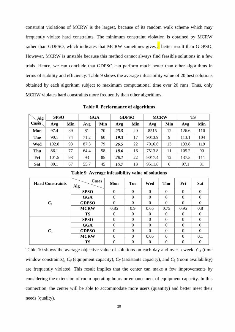
searching process highly fluctuated. The convergence of all other algorithms is also shown in

Figure 13. The figure shows the minimal cost of constraint violation in each generation of other

0

20

40

60

80

100

120

140

160

1 3 5 7 9 11 13 15 17 19 21 23 25 27 29 31 33 35 37 39

No.

of

con

stra

int

vio

lati

on

No. of generations

DPSO1

DPSO2

DPSO3

GDPSO

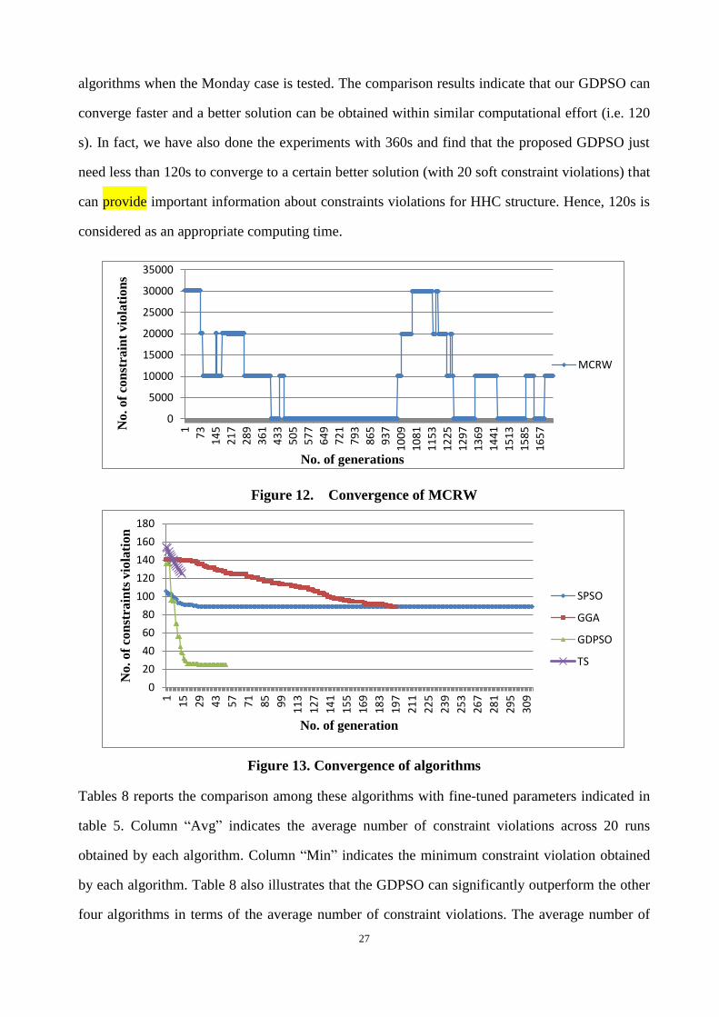
27

algorithms when the Monday case is tested. The comparison results indicate that our GDPSO can

converge faster and a better solution can be obtained within similar computational effort (i.e. 120

s). In fact, we have also done the experiments with 360s and find that the proposed GDPSO just

need less than 120s to converge to a certain better solution (with 20 soft constraint violations) that

can provide important information about constraints violations for HHC structure. Hence, 120s is

considered as an appropriate computing time.

Figure 12. Convergence of MCRW

Figure 13. Convergence of algorithms

Tables 8 reports the comparison among these algorithms with fine-tuned parameters indicated in

table 5. Column “Avg” indicates the average number of constraint violations across 20 runs

obtained by each algorithm. Column “Min” indicates the minimum constraint violation obtained

by each algorithm. Table 8 also illustrates that the GDPSO can significantly outperform the other

four algorithms in terms of the average number of constraint violations. The average number of

0

5000

10000

15000

20000

25000

30000

35000

1

73

14

5

21

7

28

9

36

1

43

3

50

5

57

7

64

9

72

1

79

3

86

5

93

7

10

09

10

81

11

53

12

25

12

97

13

69

14

41

15

13

15

85

16

57N

o.

of

con

stra

int

vio

lati

on

s

No. of generations

MCRW

0

20

40

60

80

100

120

140

160

180

1

15

29

43

57

71

85

99

11

3

12

7

14

1

15

5

16

9

18

3

19

7

21

1

22

5

23

9

25

3

26

7

28

1

29

5

30

9

No.

of

con

stra

ints

vio

lati

on

No. of generation

SPSO

GGA

GDPSO

TS

28

constraint violations of MCRW is the largest, because of its random walk scheme which may

frequently violate hard constraints. The minimum constraint violation is obtained by MCRW

rather than GDPSO, which indicates that MCRW sometimes gives a better result than GDPSO.

However, MCRW is unstable because this method cannot always find feasible solutions in a few

trials. Hence, we can conclude that GDPSO can perform much better than other algorithms in

terms of stability and efficiency. Table 9 shows the average infeasibility value of 20 best solutions

obtained by each algorithm subject to maximum computational time over 20 runs. Thus, only

MCRW violates hard constraints more frequently than other algorithms.

Table 8. Performance of algorithms

Alg

Cases

SPSO GGA GDPSO MCRW TS

Avg Min Avg Min Avg Min Avg Min Avg Min

Mon 97.4 89 81 70 23.5 20 8515 12 126.6 110

Tue 90.1 74 71.2 60 19.3 17 9013.9 9 113.1 104

Wed 102.8 93 87.3 79 26.5 22 7016.6 13 133.8 119

Thu 86.1 77 64.4 58 18.6 16 7513.8 11 105.2 90

Fri 101.5 93 93 85 26.1 22 9017.4 12 137.5 111

Sat 80.1 67 55.7 45 15.7 13 9511.8 6 97.1 81

Table 9. Average infeasibility value of solutions

Hard Constraints Cases

Alg Mon Tue Wed Thu Fri Sat

C1

SPSO 0 0 0 0 0 0

GGA 0 0 0 0 0 0

GDPSO 0 0 0 0 0 0

MCRW 0.85 0.9 0.65 0.75 0.95 0.8

TS 0 0 0 0 0 0

C3

SPSO 0 0 0 0 0 0

GGA 0 0 0 0 0 0

GDPSO 0 0 0 0 0 0

MCRW 0 0 0.05 0 0 0.1

TS 0 0 0 0 0 0

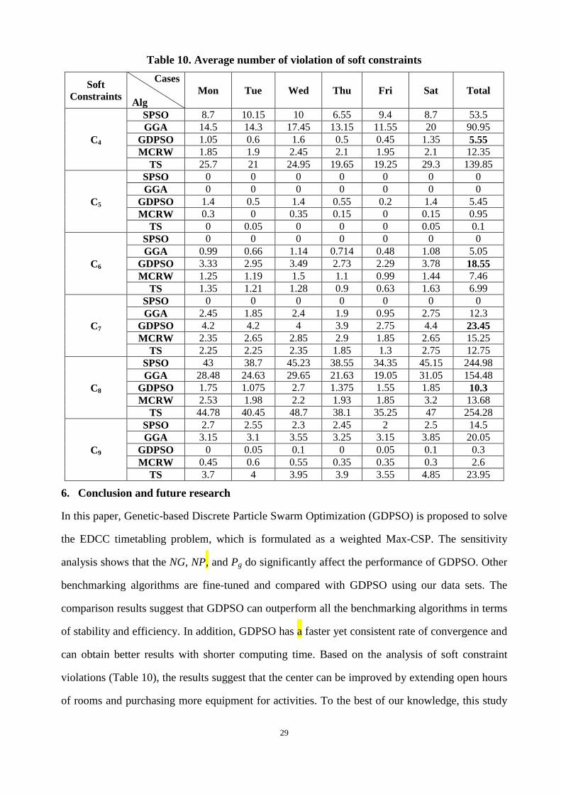
Table 10 shows the average objective value of solutions on each day and over a week. C4 (time

window constraints), C6 (equipment capacity), C7 (assistants capacity), and C8 (room availability)

are frequently violated. This result implies that the center can make a few improvements by

considering the extension of room operating hours or enhancement of equipment capacity. In this

connection, the center will be able to accommodate more users (quantity) and better meet their

needs (quality).

29

Table 10. Average number of violation of soft constraints

Soft

Constraints

Cases

Alg

Mon Tue Wed Thu Fri Sat Total

C4

SPSO 8.7 10.15 10 6.55 9.4 8.7 53.5

GGA 14.5 14.3 17.45 13.15 11.55 20 90.95

GDPSO 1.05 0.6 1.6 0.5 0.45 1.35 5.55

MCRW 1.85 1.9 2.45 2.1 1.95 2.1 12.35

TS 25.7 21 24.95 19.65 19.25 29.3 139.85

C5

SPSO 0 0 0 0 0 0 0

GGA 0 0 0 0 0 0 0

GDPSO 1.4 0.5 1.4 0.55 0.2 1.4 5.45

MCRW 0.3 0 0.35 0.15 0 0.15 0.95

TS 0 0.05 0 0 0 0.05 0.1

C6

SPSO 0 0 0 0 0 0 0

GGA 0.99 0.66 1.14 0.714 0.48 1.08 5.05

GDPSO 3.33 2.95 3.49 2.73 2.29 3.78 18.55

MCRW 1.25 1.19 1.5 1.1 0.99 1.44 7.46

TS 1.35 1.21 1.28 0.9 0.63 1.63 6.99

C7

SPSO 0 0 0 0 0 0 0

GGA 2.45 1.85 2.4 1.9 0.95 2.75 12.3

GDPSO 4.2 4.2 4 3.9 2.75 4.4 23.45

MCRW 2.35 2.65 2.85 2.9 1.85 2.65 15.25

TS 2.25 2.25 2.35 1.85 1.3 2.75 12.75

C8

SPSO 43 38.7 45.23 38.55 34.35 45.15 244.98

GGA 28.48 24.63 29.65 21.63 19.05 31.05 154.48

GDPSO 1.75 1.075 2.7 1.375 1.55 1.85 10.3

MCRW 2.53 1.98 2.2 1.93 1.85 3.2 13.68

TS 44.78 40.45 48.7 38.1 35.25 47 254.28

C9

SPSO 2.7 2.55 2.3 2.45 2 2.5 14.5

GGA 3.15 3.1 3.55 3.25 3.15 3.85 20.05

GDPSO 0 0.05 0.1 0 0.05 0.1 0.3

MCRW 0.45 0.6 0.55 0.35 0.35 0.3 2.6

TS 3.7 4 3.95 3.9 3.55 4.85 23.95

6. Conclusion and future research

In this paper, Genetic-based Discrete Particle Swarm Optimization (GDPSO) is proposed to solve

the EDCC timetabling problem, which is formulated as a weighted Max-CSP. The sensitivity

analysis shows that the NG, NP, and Pg do significantly affect the performance of GDPSO. Other

benchmarking algorithms are fine-tuned and compared with GDPSO using our data sets. The

comparison results suggest that GDPSO can outperform all the benchmarking algorithms in terms

of stability and efficiency. In addition, GDPSO has a faster yet consistent rate of convergence and

can obtain better results with shorter computing time. Based on the analysis of soft constraint

violations (Table 10), the results suggest that the center can be improved by extending open hours

of rooms and purchasing more equipment for activities. To the best of our knowledge, this study

30

is one of the few attempts to explore the potential of evolutionary algorithms in solving Max-CSP.

However, a few limitation of this study include that our problem is mainly defined with respect to

the actual setting of the local day care center and several operating features are fixed. Thus, a

more generalized EDCC problem will be studied to obtain a more generalized solution using our

proposed GDPSO.

Our future work may focus more on the testing of GDPSO on larger Max-CSP, compared with

the one reported in this paper. Moreover, the GDPSO search mechanism will be further

investigated. In this study, the computational time for each example was nearly 2 min, which

could be reduced to enhance the usefulness of our GDPSO. Finally, GDPSO can be used to solve

other real-world problems, such as vehicle routing problems for home care visits and nurse

scheduling problems in hospitals.

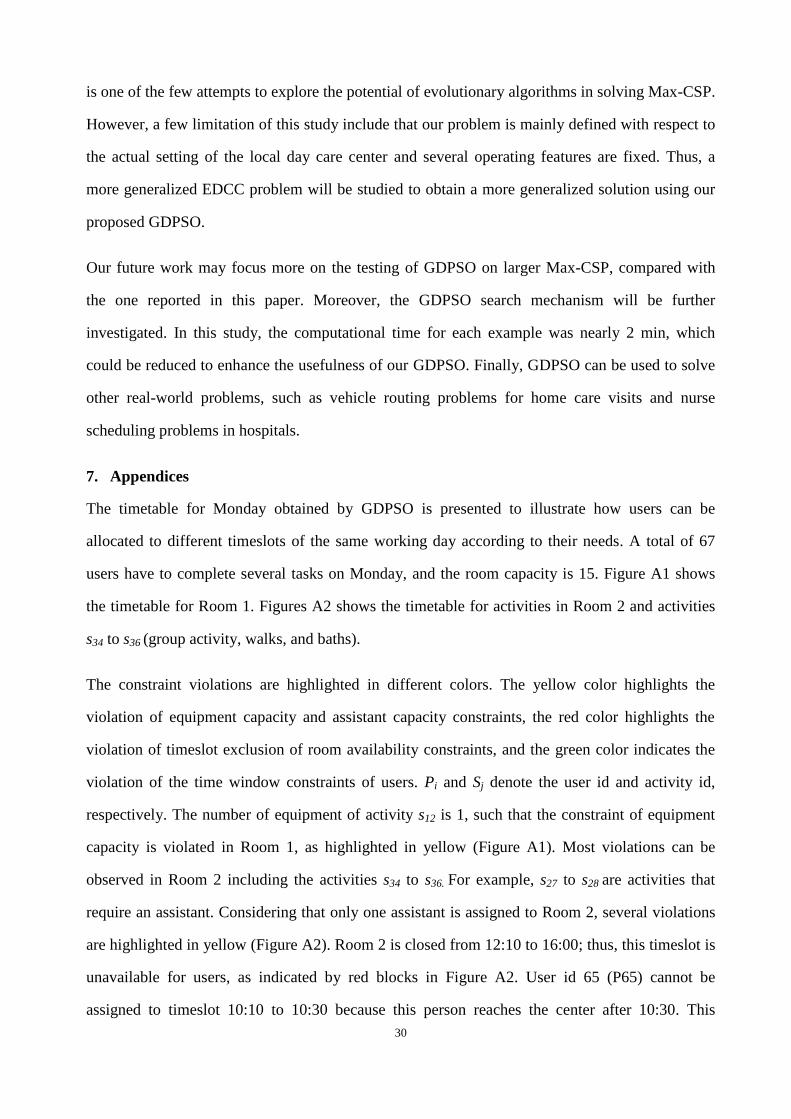
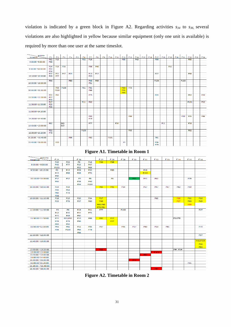
7. Appendices

The timetable for Monday obtained by GDPSO is presented to illustrate how users can be

allocated to different timeslots of the same working day according to their needs. A total of 67

users have to complete several tasks on Monday, and the room capacity is 15. Figure A1 shows

the timetable for Room 1. Figures A2 shows the timetable for activities in Room 2 and activities

s34 to s36 (group activity, walks, and baths).

The constraint violations are highlighted in different colors. The yellow color highlights the

violation of equipment capacity and assistant capacity constraints, the red color highlights the

violation of timeslot exclusion of room availability constraints, and the green color indicates the

violation of the time window constraints of users. Pi and Sj denote the user id and activity id,

respectively. The number of equipment of activity s12 is 1, such that the constraint of equipment

capacity is violated in Room 1, as highlighted in yellow (Figure A1). Most violations can be

observed in Room 2 including the activities s34 to s36. For example, s27 to s28 are activities that

require an assistant. Considering that only one assistant is assigned to Room 2, several violations

are highlighted in yellow (Figure A2). Room 2 is closed from 12:10 to 16:00; thus, this timeslot is

unavailable for users, as indicated by red blocks in Figure A2. User id 65 (P65) cannot be

assigned to timeslot 10:10 to 10:30 because this person reaches the center after 10:30. This

31

violation is indicated by a green block in Figure A2. Regarding activities s34 to s36, several

violations are also highlighted in yellow because similar equipment (only one unit is available) is

required by more than one user at the same timeslot.

Figure A1. Timetable in Room 1

Figure A2. Timetable in Room 2

32

8. Reference

[1] Christensen K, Doblhammer G, Rau R, Vaupel JW. Ageing populations: The challenges ahead.

The Lancet. 2009;374(9696):1196-208

[2] Reinhardt UE. Does the aging of the population really drive the demand for health care? Health

Affairs. 2003;22(6):27-39

[3] Solos IP, Tassopoulos IX, Beligiannis GN. A generic two-phase stochastic variable

neighborhood approach for effectively solving the nurse rostering problem. Algorithms.

2013;6(2):278-308.

[4] Della Croce F, Salassa F. A variable neighborhood search based matheuristic for nurse rostering

problems. Ann Oper Res. 2014;218(1):185-99.

[5] Santos HG, Toffolo TAM, Gomes RAM, Ribas S. Integer programming techniques for the

nurse rostering problem. Ann Oper Res. 2014:1-27.

[6] Burke EK, Curtois T. New approaches to nurse rostering benchmark instances. European

Journal of Operational Research. 2014;237(1):71-81.

[7] Tassopoulos IX, Solos IP, Beligiannis GN. Α two-phase adaptive variable neighborhood

approach for nurse rostering. Computers & Operations Research. 2015;60:150-69.

[8] Cacchiani V, Toth P. Nominal and robust train timetabling problems. European Journal of

Operational Research. 2012;219(3):727-37

[9] Jat SN, Yang SX. A hybrid genetic algorithm and tabu search approach for post enrolment

course timetabling. Journal of Scheduling. 2011;14(6):617-37.

[10] Shiau DF. A hybrid particle swarm optimization for a university course scheduling problem

with flexible preferences. Expert Systems with Applications. 2011;38(1):235-48.

[11] Yang Sx, Jat SN. Genetic algorithms with guided and local search strategies for university

course timetabling. IEEE Transactions on Systems, Man, and Cybernetics, Part C: Applications and

Reviews. 2011;41(1):93-106

[12] Ceschia S, Di Gaspero L, Schaerf A. Design, engineering, and experimental analysis of a

simulated annealing approach to the post-enrolment course timetabling problem. Computers &

Operations Research. 2012;39(7):1615-24.

[13] Tassopoulos IX, Beligiannis GN. A hybrid particle swarm optimization based algorithm for

high school timetabling problems. Applied Soft Computing. 2012;12(11):3472-89.

[14] Chen RM, Shih HF. Solving university course timetabling problems using constriction particle

swarm optimization with local search. Algorithms. 2013;6(2):227-44.

[15] Alzaqebah M, Abdullah S. Hybrid bee colony optimization for examination timetabling

problems. Computers & Operations Research. 2015;54(0):142-54.

[16] Freuder EC, Wallace RJ. Partial constraint satisfaction. Artificial Intelligence.

1992;58(1):21-70

[17] Normand JM, Goldsztejn A, Christie M, Benhamou F. A branch and bound algorithm for

numerical Max-CSP. Constraints. 2010;15(2):213-37.

[18] Minton S, Johnston MD, Philips AB, Laird P. Minimizing conflicts: A heuristic repair method

for constraint satisfaction and scheduling problems. Artificial Intelligence. 1992;58(1):161-205

[19] Galinier P, Hao JK. Tabu search for maximal constraint satisfaction problems. In: Smolka G,

(Ed.). Principles and Practice of Constraint Programming-CP97: Springer; 1997. p. 196-208

33

[20] Bouamama S, Jlifi B, Ghédira K. D2G2A: A distributed double guided genetic algorithm for

Max_CSPs. In: Palade V, Howlett RJ, Jain L, (Eds.) Knowledge-Based Intelligent Information and

Engineering Systems: Springer; 2003. p. 422-9

[21] Khadhraoui A, Bouamama S. A new hybrid distributed double guided genetic swarm

algorithm for optimization and constraint reasoning: Case of Max-CSPs. International Journal of

Swarm Intelligence Research. 2012;3(2):63-74.

[22] Tseng CT, Liao CJ. A discrete particle swarm optimization for lot-streaming flowshop

scheduling problem. European Journal of Operational Research. 2008;191(2):360-73

[23] Zhang CS, Sun JG, Zhu XJ, Yang QY. An improved particle swarm optimization algorithm for

flowshop scheduling problem. Information Processing Letters. 2008;108(4):204-9.

[24] Ponnambalam SG, Jawahar N, Chandrasekaran S. Discrete particle swarm optimization

algorithm for flowshop scheduling. In: Lazinica A, (Ed.). Particle Swarm Optimization: INTECH

Open Access Publisher; 2009.

[25] Wang XP, Tang LX. A discrete particle swarm optimization algorithm with self-adaptive

diversity control for the permutation flowshop problem with blocking. Applied Soft Computing.

2012;12(2):652-62

[26] Shao XY, Liu WQ, Liu Q, Zhang CY. Hybrid discrete particle swarm optimization for

multi-objective flexible job-shop scheduling problem. The International Journal of Advanced

Manufacturing Technology. 2013:1-17

[27] Goksal FP, Karaoglan I, Altiparmak F. A hybrid discrete particle swarm optimization for

vehicle routing problem with simultaneous pickup and delivery. Computers & Industrial

Engineering 2012.

[28] Kechagiopoulos PN, Beligiannis GN. Solving the urban transit routing problem using a

particle swarm optimization based algorithm. Applied Soft Computing. 2014;21:654-76.

[29] Ho TK, Tsang CW, Ip KH, Kwan KS. Train service timetabling in railway open markets by

particle swarm optimisation. Expert Systems with Applications. 2012;39(1):861-8.

[30] Bratton D, Kennedy J. Defining a standard for particle swarm optimization. the 4th Swarm

Intelligence Symposium (SIS'07). Honolulu, Hawaii, USA: IEEE; 2007. p. 120-7.

[31] Burke EK, Kingston J. Applications to timetabling. In: Gross JL, Yellen J, (Eds.) Handbook of

graph theory: CRC Press; 2004. p. 445.

[32] Pillay N. A survey of school timetabling research. Ann Oper Res. 2014;218(1):261-93.

[33] MirHassani SA, Habibi F. Solution approaches to the course timetabling problem. Artificial

Intelligence Review. 2013;39(2):133-49.

[34] Qu R, Burke EK, McCollum B, Merlot LTG, Lee SY. A survey of search methodologies and

automated system development for examination timetabling. Journal of scheduling.

2009;12(1):55-89.

[35] Ribeiro CC. Sports scheduling: Problems and applications. International Transactions in

Operational Research. 2012;19(1-2):201-26

[36] Cacchiani V, Caprara A, Toth P. Scheduling extra freight trains on railway networks.

Transportation Research Part B: Methodological. 2010;44(2):215-31.

[37] Liebchen C, Möhring R. The modeling power of the periodic event scheduling problem:

Railway timetables — and beyond. In: Geraets F, Kroon L, Schoebel A, Wagner D, Zaroliagis C,

(Eds.) Algorithmic Methods for Railway Optimization: Springer Berlin Heidelberg; 2007. p. 3-40.

34

[38] Phillips AE, Waterer H, Ehrgott M, Ryan DM. Integer programming methods for large-scale

practical classroom assignment problems. Computers & Operations Research. 2015;53:42-53.

[39] He F, Qu R. A constraint programming based column generation approach to nurse rostering

problems. Computers & Operations Research. 2012;39(12):3331-43.

[40] Eberhart R, Kennedy J. A new optimizer using particle swarm theory. the 6th International

Symposium on Micro Machine and Human Science (MHS '95). Nagoya, Japan: IEEE; 1995. p.

39-43

[41] Akjiratikarl C, Yenradee P, Drake PR. An improved particle swarm optimization algorithm for

care worker scheduling. Industrial Engineeering & Management Systems. 2008;7(2):171-81.

[42] Liu B, Wang L, Jin YH. An effective PSO-based memetic algorithm for flow shop scheduling.

IEEE Transactions on Systems, Man, and Cybernetics, Part B: Cybernetics. 2007;37(1):18-27

[43] Zhang H, Li XD, Li H, Huang FL. Particle swarm optimization-based schemes for

resource-constrained project scheduling. Automation in Construction. 2005;14(3):393-404.

[44] Jonsson P, Krokhin A, Kuivinen F. Ruling out polynomial-time approximation schemes for

hard constraint satisfaction problems. In: Diekert V, Volkov M, Voronkov A, (Eds.) Computer

Science – Theory and Applications: Springer Berlin Heidelberg; 2007. p. 182-93.

[45] Sharapov RR. Genetic algorithms: Basic ideas, variants and analysis. In: Obinata G, Dutta A,

(Eds.) Vision Systems: Segmentation and Pattern Recognition: INTECH Open Access Publisher;

2007.

[46] Montgomery DC. Design and analysis of experiments: Wiley New York; 1984.