Genetic Analysis of Complex Diseases || Data Analysis Issues in Expression Profiling

&CHAPTER 7

Data Analysis Issues in ExpressionProfiling

SIMON LIN and MICHAEL HAUSER

INTRODUCTION

Although virtually every cell in the body contains the full complement of genes,

individual cells and tissues are distinguished from one another by the subset of

RNA or protein products of those genes they express. Expression profiling enables

identification of this subset of transcribed genes and the levels at which they are

expressed, thereby providing a valuable tool for increasing our understanding of

the regulatory and functional complexities of the genome. Expression profiling

has been used to characterize signaling and regulatory pathways, identifying

genes responsive to p53 induction (Zhao et al., 2000; Madden et al., 1997) and

genes expressed in yeast during sporulation (Chu et al., 1998). Much research has

focused on using gene expression information to distinguish between different

classes of malignant tissue: Diffuse large B-cell lymphomas that respond well to

chemotherapy can be distinguished from those that do not on the basis of expression

profiling (Alizadeh et al., 2000). Similar approaches have been taken to analyze

breast cancer (Perou et al., 2000) and colon cancer (Alon et al., 1999; Zhang

et al., 1997). This use of expression analysis to segregate samples into distinct phe-

notypic groups, called classification analysis, has the potential to greatly improve

clinical management of cancer.

Another powerful use of gene expression profiling is the identification of candi-

date susceptibility genes for complex diseases. Linkage analysis in such disorders

frequently identifies large genomic regions that may contain hundreds of genes.

Sorting through so many genes to find the few that influence disease susceptibility

can be a daunting task. Expression profiling reveals genes whose expression levels

are up or down regulated as a function of the disease process or in response to acute

disease-related stimuli. Genes with such a pattern of expression that also map to

193

Genetic Analysis of Complex Diseases, Second Edition, Edited by Jonathan L. Haines andMargaret Pericak-VanceCopyright # 2006 John Wiley & Sons, Inc.

regions of linkage represent excellent candidates for further molecular analysis. This

strategy has been used in conjunction with rat model systems to generate a series of

excellent candidate susceptibility genes for mania and psychosis (Niculescu et al.,

2000).

Many different experimental methods have been used for expression profiling.

All methods begin with the purification of transcribed RNA from the tissue

sample(s) of interest. The classic techniques of subtractive hybridization (Lee

et al., 1991) and differential display (Liang and Pardee, 1992) use physical

methods to isolate and clone messages whose expression levels differ greatly

between two samples. In this chapter, we will focus on the two techniques

that have emerged as the most powerful and flexible experimental approaches

to expression analysis: serial analysis of gene expression (SAGE) (Velculescu

et al., 1995) and microarray analysis. These two techniques have the great advan-

tage that they generate large databases of expression information, rather than just a

few clones for immediate analysis. A single experiment can provide information

about the expression levels of thousands of genes in a given sample. These

expression data are now being stored in public databases, providing a tremen-

dously rich source of information that can be mined repeatedly by many different

investigators.

In this chapter, we will first describe the construction and analysis of SAGE

libraries. Then, after a brief description of the different types of DNA microarrays,

we will introduce some more advanced approaches to the statistical analysis of com-

plex expression datasets obtained through SAGE or microarrays. Finally, we will

discuss some biological applications of these expression profiling techniques.

SERIAL ANALYSIS OF GENE EXPRESSION

Developed in 1995 by Vogelstein and Kinzler (Velculescu et al., 1995), briefly,

SAGE isolates a 14-bp sequence immediately adjacent to the 30-most N1aIII site

within each transcript. These short sequences, called tags, are then cloned in long

tandem arrays for sequencing. The approach is conceptually similar to sequencing

large numbers of cDNA clones from a tissue but is much more efficient as more

than 20 tags can be identified by sequencing a single template. The genes to

which the SAGE tags correspond are then identified by using the “tag to gene map-

ping” database prepared by Alex Lash, available on the National Center for

Biotechnology Information (NCBI) website (http://www.ncbi.nlm.nih.gov/SAGE/SAGEtag.cgi). Our current knowledge of the human genome allows the

majority of SAGE tags to be mapped to a single UniGene set. The UniGene sets

are clusters of mRNA and expressed sequence tags (ESTs) that are believed to rep-

resent individual genes. A subset of SAGE tags map to multiple UniGene sets,

which may reflect uncertainty in transcript clustering in the UniGene sets, actual

sequence similarity causing different genes to have the same SAGE tag, or complex-

ities of transcript processing, including alternative splicing or polyadenylation sites.

The expression patterns of many transcripts can be evaluated by sequencing several

194 DATA ANALYSIS ISSUES IN EXPRESSION PROFILING

thousand clones (40,000–50,000 tags), comparing the abundance of individual tags,

and identifying the corresponding genes.

The detailed SAGE protocol is freely available for academic use and can be

obtained from http://www.sagenet.org/sage.htm. This technique has several

important advantages as compared to other techniques for the detection of tissue-

specific expression. First, SAGE does not simply isolate a small number of

clones, but rather creates a permanent, quantitative record of the entire set of

sequences transcribed in a given tissue or cell population. Thus, a SAGE database

can be used long after it was originally constructed to ascertain the expression

levels of newly identified genes. Second, SAGE can detect small changes in

expression levels, even among messages that are expressed at very low levels over-

all. Third, transcripts that are over- or underexpressed can be detected equally well.

SAGE is an “open-platform” technology: It does not require any preexisting biologi-

cal or sequence information and can be applied to any species. In contrast, micro-

array experiments cannot detect a transcript unless the corresponding gene is

already known and has been included in the array. Other open-platform systems

for analysis of gene expression such as GeneCalling, TOGA, and READS have

been recently reviewed (Green et al., 2001).

Since the original SAGE protocol was published in 1995, many technical

improvements have been introduced. Using the I-SAGE kit marketed by Invitrogen

(Carlsbad, CA), SAGE can now be performed starting with as little as 2 mg total

RNA. Additional modifications allow SAGE libraries to be constructed from as

few as 40,000 cells (Datson et al., 1999; Virlon et al., 1999; Peters et al., 1999) or,

with the addition of a polymerase chain reaction (PCR) amplification step, from a

single oocyte (Neilson et al., 2000). The sequencing of several thousand clones

from each SAGE library can now be performed commercially on a fee-for-service

basis (Genome Therapeutics Co.). There have also been improvements in the soft-

ware used for extraction of SAGE tags from individual sequence reads. For example,

eSAGE (Margulies and Innis, 2000) allows the user to establish a minimum PHRED

quality score for each extracted SAGE tag. This allows quantitative calculations of

the frequency of sequencing errors and resulting misspecification of genes.

Analysis of SAGE Libraries

The SAGE libraries are most commonly analyzed by performing a direct compari-

son of tag abundance between two individual libraries or two groups of libraries

using software such as the xProfiler (http://www3.ncbi.nlm.nih.gov/SAGE/sagexpsetup.cgi). The statistical significance of observed differences in tag counts

between SAGE libraries can be evaluated in several different ways. Monte Carlo

simulations can be used to estimate the likelihood that the experimentally observed

differences could arise by chance alone (Zhang et al., 1997). An alternate Bayesian

approach has been suggested (Audic and Claverie, 1997), and the necessary soft-

ware has been made available (http://igs-server.cnrs.mrs.fr). Analysis of SAGE

data using simple hypothesis-testing methods such as x2 or the Fisher exact test

has been reviewed (Man et al., 2000).

SERIAL ANALYSIS OF GENE EXPRESSION 195

The amount of SAGE data in public databases is increasing rapidly through the

efforts of groups such as the Cancer Genome Anatomy Project (CGAP, http://cgap.nci.nih.gov/). Well over 300 libraries have now been constructed from

normal and malignant tissue (Lal et al., 1999). As more libraries are constructed

from different tissue types, these databases can be used for surveys of tissue-specific

expression of individual genes, sometimes called digital northern analysis (http://www.ncbi.nlm.nih.gov/SAGE/sagevn.cgi). The availability of large amounts of

SAGE data will also allow the application of the more sophisticated dimensional

reduction and clustering technologies described below.

Microarray Analysis

In contrast to SAGE, microarray technologies are all based on mRNA hybridization,

so only genes with available sequences or clones can be detected. First, polyA

mRNA is isolated from samples and labeled with fluorescent dye or a radioactive

isotope. It is then hybridized to probe sequences arrayed at high density on a

solid support (glass, silicon, or nylon membrane). Finally, a scanner measures the

fluorescent intensities of each spot on the hybridization array, from which the initial

concentrations of the corresponding transcripts are inferred. There are two main

types of microarrays: commercial high-density oligonucleotide arrays, called

“gene chips,” and custom-spotted glass slides.

Affymetrix Corporation (Santa Clara, CA) manufactures high-density gene chips

using photolithographic technology. In general, the specific gene probes found on

these arrays are standardized and cannot be customized for individual users. Each

probe set consists of over 20 different oligonucleotides, some matching the tran-

script’s sequence exactly and some containing intentional mismatches as back-

ground hybridization controls. Proprietary software algorithms provided by the

manufacturer use the level of hybridization to all of these oligonucleotides to calcu-

late the level of gene expression in a sample.

Custom-spotted glass slide microarrays can be prepared by individual users or

core laboratories. Large collections of transcripts of individual genes (PCR products

or long oligonucleotides) are available from commercial sources such as Invitrogen

Corporation (Carlsbad, CA). Individual transcripts are selected from these probe sets

and a small volume of each corresponding DNA solution is spotted onto a glass

slide, where it adheres tightly. These glass slides are then hybridized and scanned

to quantitate RNA abundance.

Oligonucleotide gene chips are manufactured with a consistent amount of hybridi-

zation target at each spot on each chip. For this reason, a chip can be probed with a

single RNA sample, and the resulting gene expression levels can be compared with

other independent chip experiments after appropriate normalization. To account for

variations in the amount of material spotted on each array, custom-spotted glass

slide arrays are hybridized with two different RNA samples simultaneously, one

experimental and one reference sample. The two samples are labeled with different

fluorescent dyes, and the expression data obtained are a ratio of the two samples.

Microarray data analysis consists of three steps: (i) data preparation, in which

data are adjusted for the downstream algorithms; (ii) algorithm selection for data


analysis; and (iii) interpretation, in which the results from the algorithms are

explained in a biological context.

Data Preparation

Data preparation is a critical step in microarray data analysis. Each data preproces-

sing method can accentuate, create, or destroy findings from downstream analytic

algorithms. It has been argued that data preprocessing has had a stronger influence

on the final results than the choices of subsequence statistical analysis methods

(Hoffmann et al., 2002). Data quality control, transformation, and normalization

are usually addressed in this step.

Data Quality Control. Expression profiling measurements usually contain noise

and erroneous data points, due to scratches on the hybridization surface, white noise

during image scanning, irregular spot morphology, and numerous other stochastic

experimental artifacts. The first step in data analysis is quality control to identify

those erroneous data points. Flagging such points and eliminating them from further

analysis can improve the overall quality of the analysis. More sophisticated algor-

ithms have been developed to quantitatively measure spot qualities (Wang et al.,

2001). Li and Wong (2001) have proposed a statistical model to detect outliers

and data irregularities for the Affymetrix platform. It has been shown that quality

control of the raw data helps normalization and downstream analysis (Yang et al.,

2001; Raffelsberger et al., 2002).

Data Transformation. Many statistical tests such as the t-test and analysis of

variance (ANOVA) assume independence between the mean and the variance of

data. However, raw measurements of microarrays usually demonstrate a reasonably

strong correlation between the mean expression level of a given gene and its stan-

dard deviation (Durbin et al., 2002). Thus, a transformation is necessary to stabilize

the variance, such as logarithm transformations (Dudoit et al., 2002) and cubic-root

transformations (Tusher et al., 2001). However, log transformations inflate the var-

iance of observations at low expression levels. Rocke (Durbin et al., 2002) and

Huber (2002) independently proposed similar models for microarray data transform-

ation to stabilize the variance over the full range of measurements.

Data Normalization. Before any numerical inference about microarray data can

be made, it must be clear that those measurements reflect true biological differences,

not experimental artifacts such as dye-labeling effects, array-printing pin effects, or

overall intensity differences. Those systematic differences caused by experimental

artifacts can be eliminated by a normalization procedure. The assumptions of nor-

malization are usually based on constant expression levels of internal housekeeping

genes or external markers, overall intensity levels, or constant expression of the

majority of genes (Yang et al., 2002; Kepler et al., 2002). Huber et al. (2002)

consolidated both data normalization and variance into one variance stabilization

and normalization (VSN) model.


Expression Data Matrix

Before we discuss data analysis in more detail, we must first define several concepts

used in multivariate analysis and pattern recognition. An object is a sample posses-

sing quantitative or qualitative properties that can be described by features, also

known as attributes or variables. A series of observations made on a set of objects

can be organized as a multivariate data matrix—a rectangular array of numbers.

Here we use the convention that lets the rows of the matrix represent objects and

the columns represent features. The general data matrix X with m objects and n

features can be written as follows:

X ¼

x11 � � � x1 j � � � x1n

..

. . .. ..

. . .. ..

.

xi1 � � � xi j � � � xin

..

. . .. ..

. . .. ..

.

xm1 � � � xm j � � � xm n

266666664

377777775

The element in row i and column j of matrix X is denoted xij. It represents the

value of an object i on feature j. A vector is a special matrix with a single column

or a single row of elements. Thus, rows or columns in a matrix can be viewed as

vectors.

In the gene expression data matrix, by convention the objects (rows) in the matrix

are genes and the features (columns) in the matrix are experimental conditions.

Usually, m, the number of genes, is much larger than n, the number of experimental

conditions. In this orientation, a complete row of features is called a gene’s profile. It

is expressed as a vector in the n-dimensional feature space. Similarly, a column

represents an experiment’s profile by a vector in the m-dimensional gene space.

This orientation of the expression data matrix is commonly used for clustering

genes into functional groups in response to experimental stimuli. If necessary, the

data matrix can be transposed so that the columns represent genes while the rows

represent experiments (or patients). Such an arrangement is often used in supervised

learning to classify the gene expression profiles of patients.

In addition to feature measurements, there is also a priori knowledge of the

objects. This external knowledge is called a label. For example, if we measure

gene expression features of each patient by microarrays, the known diagnostic

category to which a patient belongs is the label. Note that in this case a label

is acquired by the physician, independently from the features acquired by micro-

arrays. In supervised machine learning, labels are required in the training session,

so that unknown samples can subsequently be classified into predefined groups.

Unsupervised machine learning (clustering) does not require labels.

Dimension Reduction of Features

To reduce the complexity of the dataset, the objects in the n-dimensional space can

be mapped into a lower dimensional space. This procedure is always applied before


feeding data into a machine-learning algorithm. Although it may seem counter-

intuitive to present fewer features to the machine-learning algorithm, dimension

reduction is necessary for two reasons. First, the “curse of dimensionality” (see

below) prohibits higher dimensional data from being fed into the machine-learning

process. Second, objects can only be visualized when the dimension is less than 3.

Dimension reduction is achievable by selecting existing features based on expert

knowledge, statistical algorithms (Fowlkes et al., 1987), or by creating new features

using dimension reduction algorithms such as principal-component analysis or

multidimensional scaling.

Curse of Dimensionality. In studies of disease classification based on micro-

array data, there tend to be too many molecular features for each patient, given

the small sample size of patients. There is a temptation to throw everything into

the machine-learning algorithm, but extra features that are unrelated to the classi-

fication tend to dilute the analysis and cause the algorithm to run astray. This is

called the “curse of dimensionality.” In machine learning, the size of the search

space increases exponentially with the dimension of features to model. Thus, the

reduction of the features is crucial to circumvent the curse of dimensionality. Vari-

able selection prior to clustering is discussed by Fowlkes et al. (1987). In super-

vised machine learning, it is recommended that the number of the training

samples per class be at least 5–10 times the number of features (Jain and

Chandrasekaran, 1982).

Principal-Component Analysis. Principal-component analysis (PCA) reduces

the number of features by forming new features to describe objects in lower dimen-

sions (Jolliffe, 1986). These new features are labeled principal components, which

are linear combinations of the original features. The same idea is also known as

Karhunen–Loeve transformation in signal processing and singular-value deposition

(SVD) in matrix computation. The principal components have two properties. First,

the new components are orthogonal to each other. This indicates that the correlation

between the original features has been removed. Second, the principal components

have decreasing ability to explain variance in the dataset. The first principal com-

ponent explains the largest variance of the objects. As the cardinality of the principal

components increases, the explained variance in the dataset decreases. It is often the

case that a small number of the early components are sufficient to represent most of

the variations in the data.

The orthogonal characteristic of the principal components was exploited by Alter

et al. (2000) in the hope of categorizing genes into orthogonal signal transduction

pathways. The decreasing importance of the principal components makes it possible

to ignore low-impact components with very little loss of information. Principal-

component analysis has been used as a means to filter out the noise and to

remove redundancy in the dataset (Hilsenbeck et al., 1999).

Multidimensional Scaling. Unlike PCA, multidimensional scaling (MDS) uses

the distance between objects as a starting point for analysis, rather than the direct


observation of objects in the n-dimensional space. It attempts to represent a multi-

dimensional dataset in two or three dimensions such that the distance between

objects in the original n-dimensional space is preserved as faithfully as possible

in the projected space. A simple example is to construct a map of Virginia

using only road distances between the towns. Multidimensional scaling can

be achieved by the principal coordinate algorithm (Gower, 1966) to minimize

the variance or by the spring-embedding algorithm (Kruskal, 1964) to minimize

the stress. It is the process of visualizing relationships between objects so that

human experts can interpret the data. If the data are projected in one dimension,

then the ordering of objects is seriated according to their similarities. The

application of MDS to microarray data will be discussed in the visualization

section below.

Measures of Similarity between Objects

To study the degree of resemblance in the objects, many different mathematical

functions are suggested as similarity measures. The most common ones, Euclidean

distance and Pearson correlation, are described here. A different choice of similarity

measure can lead to a very different interpretation of expression data (Getz et al.,

2000).

Euclidean Distance. If objects are geometrically represented as points in an

n-dimensional feature space, their proximities can be measured as the distance

between pairs of points. Euclidean distance is the square root of the sum of the

squared difference between two objects across n features. The Euclidean distance

Dij between object i and object j is represented by

Dij ¼

ffiffiffiffiffiffiffiffiffiffiffiffiffiffiffiffiffiffiffiffiffiffiffiffiffiffiffiffiffiXn

k¼1

(xik � x jk)2

s

where xik denotes the measurement of object i on feature k, xjk denotes the measure-

ment of object j on feature k, and n is the dimension.

In microarray analysis, Euclidean distance is used to contrast the difference in the

absolute expression level of two objects. For example, the absolute expression level

of a group of genes can be significantly higher in malignant tumors than in benign

tumors, even though their relative shapes as measured by the Pearson correlation

coefficient are the same. In this case, Euclidean distance is more appropriate to

measure the differences than the Pearson correlation coefficient.

Pearson Coefficient. The Pearson product-moment correlation, or Pearson

correlation, is the dot product of two normalized vectors. It ranges from þ1 to

21. A correlation of þ1 conveys a perfect positive linear relationship; a correlation

of 21 conveys a perfect negative linear relationship; a correlation of zero indicated


that there is no linear relationship. The Pearson coefficient Qij between object i and

object j is represented by

Qij ¼

Pnk¼1 (xik � xi)(x jk � xj)ffiffiffiffiffiffiffiffiffiffiffiffiffiffiffiffiffiffiffiffiffiffiffiffiffiffiffiffiffiffiffiffiPn

k¼1 (xik � xi)2

q ffiffiffiffiffiffiffiffiffiffiffiffiffiffiffiffiffiffiffiffiffiffiffiffiffiffiffiffiffiffiffiffiPnk¼1 (x jk � xj)

2q

where xi and xj are the vector profile means of objects i and j, respectively. The

denominator terms represent the scatter. Pearson correlation stresses the similarity

between the “shape” of two expression profile vectors and ignores the differences

in their absolute magnitudes. This corresponds to the biological notion of two

coexpressed genes (Eisen et al., 1998).

The difference between the Euclidian distance and the Pearson correlation also

depends on the rescaling of the vectors. When the Euclidean distance is calculated

on vectors normalized by zero mean and unit variance transformation, discrimi-

nation of elevation and scatter is lost, making the distance closely related to the

Pearson correlation (Skinner, 1978).

Unsupervised Machine Learning: Clustering

Clustering uses a collection of unsupervised machine-learning algorithms to group

objects into subsets based on their similarities. By revealing these natural groupings

in a large dataset, cluster analysis provides an intuitive way to reduce data complex-

ity from m objects to k groups. Clustering does not rely on any previous knowledge

of the dataset (no label information is required before clustering); neither does it

require a training process. In this sense, it is “unsupervised” learning. Cluster analy-

sis is widely used in biological sciences such as numerical taxonomy (Sneath and

Sokal, 1973) and evolution analysis (Fitch and Margoliash, 1967). It is also an

appealing approach to microarray data analysis because it promises to find patterns

without a priori knowledge of the data.

What to Cluster. Clustering methods can be used to group genes that have similar

profiles across a range of experimental conditions. Alternatively, experimental con-

ditions in the m-dimensional gene space can be clustered according to their gene

expression profiles. Two-way clustering groups both the row and column vectors;

it can be done independently by using a two-stage approach (Perou et al., 2000)

or by considering both row and column vectors at the same time during clustering

(Getz et al., 2000).

Hierarchical Clustering. The hierarchical algorithm results in a treelike rep-

resentation of the data, often called a dendrogram. It enables an analyst to observe

how objects are being merged or split into groups. The process of forming the hier-

archy can be “bottom up” or “top down.” Agglomerative clustering starts with each

object in its own cluster. The objects then merge into more and more coarse-grained

clusters until all objects are in a single cluster. Divisive clustering reverses this


process. It starts with all objects in one cluster and subdivides them into many

fine-grained clusters.

Most clustering algorithms work agglomeratively. They iteratively join the

objects into a tree structure. First, all of the objects are in their own cluster. Then,

a heuristic rule is applied to find the “best” pair for merging. The merged

clusters then replace the original ones. This process is repeated until only one cluster

remains. Algorithms differ in the heuristics used to define the best pair of clusters to

merge. Single-linkage, average-linkage, and complete-linkage algorithms all use the

minimum-distance criterion. Single linkage defines the distance as the single short-

est link between clusters. Complete linkage takes the distance between the most dis-

tant members, and average linkage uses the average distance between the two cluster

centers. An alternative to the distance-based rule, Ward’s method uses the sum-of-

squares criterion. This criterion chooses the cluster to be merged based on the smal-

lest increase in the within-group sum of squares.

Given the heuristic algorithm rules described above, users choose an algorithm

for a specific purpose. Single linkage often finds large undesirable serpentine clus-

ters, where the chained objects at the opposite ends of the same cluster may be dis-

similar. Thus, single linkage is incapable of delineating poorly separated clusters.

On the opposite end of the spectrum, complete linkage tends to find excessively

small and compact clusters. Average linkage, sometimes used as a compromise

between single and complete linkage, is sensitive to the transformation of the dis-

tance metrics. In other words, the dendrogram resulting from the average-linkage

method might be different if a different transformation is applied to the raw

measurements. Different algorithms can reveal different facets of the dataset and

may have the potential to complement each other.

Partitional Clustering. Hierarchical clustering, as described above, results in a

nested structure of groupings. In contrast, partitional clustering, such as k-means

(MacQueen, 1967), simply divides the objects into k groups without giving any

details of subgrouping within each group. It is especially appropriate when the

desired number of groups, k, is known. The algorithm achieves the partition itera-

tively. Initially, all the objects are assigned at random to the k groups. Then the cen-

troid of each group is computed, the distance of each object to the centroids is

recalculated, and each object is assigned to one of the nearest cluster centroids.

These two steps are alternated until a convergence criterion is met. Computationally,

k-means clustering is less expensive in terms of time and memory consumption than

hierarchical clustering. However, in hierarchical clustering, there is no need to

specify the number of classes k. One should be aware that due to the iterative

nature of k-means algorithm, the initial order of the objects influences the results;

the results will be slightly different with each run. Examples of k-means clustering

can be found in Ishida et al. (2002) and Brar et al. (2001).

Self-Organizing Map. Kohonen’s self-organizing map (SOM) algorithm

(Kohonen, 1995) clusters data by taking advantage of the robustness of neural

network techniques and has been applied to messy datasets with outliers. The


SOM maps unordered objects to nodes in a one- or two-dimensional grid, such that

similar objects are assigned to the same node and similar nodes are topologically

close to each other. Chu et al. (1998; online supplement) used a one-dimensional

SOM grid to order genes during sporulation, revealing a pattern: The top fourth

of the genes are repressed at early time points and then released, while the

bottom fourth of the genes are either repressed or reduced at early time points

and highly induced at later time points.

Fuzzy Clustering. All the clustering methods described above are exclusive par-

titions, where no objects belong to more than one subset or cluster. Fuzzy clustering,

which uses the degree of membership of an object to describe whether it belongs to a

cluster, allows a nonexclusive classification of objects. The degree of membership is

based on the fuzzy-set theory developed by Zadeh (1965). This theory conceptually

modeled touching or overlapping clusters that do not have well-defined boundaries.

A fuzzy-clustering algorithm is fuzzy c-means (Cannon et al., 1986). Gasch and

Eisen (2002) demonstrated the relevance of overlapping cluster assignments to

the conditional coregulation of yeast genes.

Cluster Validity. The results of many clustering algorithms vary with the choice

of parameters. For example, when a hierarchical clustering procedure is applied,

where is the best cutting level? How does one determine k in k-means? Should

these clustering results be believed? Those are the determinants of cluster validity.

Although a visual inspection can help to validate the clustering results, a numeric

measure of cluster validity is required in many cases.

Internal Validity of Clusters. Separability can be used as an internal validation

measurement of clustering results. Davies and Bouldin (1979) developed an index to

indicate the compactness and separation of clusters. A minimum within-cluster

scatter and a maximum between-class separation will yield a lower number on the

Davies–Bouldin (DB) index, which indicates superior clustering. For k-means

clustering, a plot of DB against k will help to identify the best k for clustering.

External Validity. The goal of cluster analysis is to classify objects into meaning-

ful subsets in a biological context. External validation of clusters utilizes infor-

mation from labels to determine this. Information from labels is an independent

source of the features used in clustering. In Spellman et al. (1998), the existence

of the MCB element is used as a label to validate the G1 cluster. For the genes in

the G1 cluster, 58% (vs. 6% in control) have a copy of the perfect MCB element.

This element is bound by MBF, whose activity depends on cyclin activation. A

formal way to assess the support of a priori labeling of a certain partition is to

use Hubert’s G statistics (Hubert and Arabie, 1985).

Stability. Resampling techniques can be used to check the stability of clustering.

Robust clusters are less likely to be the result of a sample artifact or fluctuation.

Felsenstein (1985) used bootstrapping (Efron and Tibshirani, 1993) to estimate


the confidence of a dendrogram, which was followed up by Efron et al. (1996). A

discussion of the use of bootstrapping to assess the stability of hierarchical clustering

of microarray data can be found in Zhang and Zhao (2000).

Conceptualization from Clusters. In Spellman et al. (1998), expression infor-

mation regarding 800 genes is reduced to a smaller number of exemplar groups by

clustering. The authors further conceptualized the clusters into an MCM cluster,

MET cluster, histone cluster, etc. These concepts extracted from clusters are easy

to understand and remember. They greatly facilitate communication and under-

standing of the biology. Text data mining strategies can also help the conceptualiz-

ation process. Inpharmix (Greenwood, IN) software searches the MEDLINE

literature database to find conceptual schema in a list of genes identified in the

same cluster.

Implementation Strategies. There are a large number of clustering methods

reported in the literature. Readers can always get freeware executables from the

individual authors (Eisen et al., 1998; Tamayo et al., 1999) or they can code

based on the published algorithm. Several commercial data analysis packages pro-

vide a collection of documented and tested programs for clustering: SAS (RTP, NC),

S-plus (Seattle, WA), and Clustan (Edinburgh, UK). There are also software tools

that are specifically designed for analyzing microarray data, such as GeneSpring

(Redwood City, CA), BioDiscovery (Los Angeles, CA), Partek (St. Charles, MI),

and SpotFire (Cambridge, MA). The final choice of analysis methods is affected

by the investigation goal, the availability of the software, and the computational

complexity of the algorithm.

Supervised Machine Learning

The problem of supervised machine learning can be stated as follows: Given a train-

ing set of samples with known classifications (labels), build a machine that can clas-

sify objects without label information. Supervised learning performs a training

process in which the system is supervised to learn the previously classified cases

by using both features and category labels. In contrast, clustering is called unsuper-

vised learning because neither a training session nor a priori category labels are used

in the partition process. Thus, the “unconstrained” nature of clustering makes it

appropriate for pattern discovery, such as finding new subclass of diseases, while

supervised machine learning is more powerful to classifiy patients according to pre-

defined diagnostic categories. The current challenge is to classify patients according

to their clinical, morphological, and chemical data along with their molecular

expression data.

What to Classify. In supervised learning of microarray analysis, the objects for

classification are usually patient microarray experiments or biological samples

under varying conditions. For example, m patients may be described by their gene


expression profile as a vector with n dimensions, each dimension a gene. The goal is

to classify the patients in the n-dimensional space.

Linear Discriminant Analysis. Mathematically, a classifier is a mapping of m

objects in a set X to a much smaller set C of k classes. Thus, a classifier is a mapping

function

f : X �! C

where the input to the function f is the pattern of an object and the output is a

decision on its classification. The simplest mapping can be achieved by a linear dis-

criminant function that takes a linear combination of the features from the input and

correlates them with the output categories. This is called linear discriminant analysis

(LDA). The discriminant function L can be written as

L ¼ b1x1 þ b2x2 þ b3x3 þ � � � þ bnxn

where L is the LDA score, x1, x2, . . . , xn are the features of object x, and b1, b2, . . . ,

bn are the weights. The discriminant function L defines a hyperplane that separates

the objects into classes. In a simple case of classifying x into one of the two cat-

egories, a cutoff point c can be used to make the classification decision. If L � c,

then object x belongs to category 1; otherwise, it belongs to category 2. In cases

where the input is not linearly separable, LDA can fail.

k-Nearest Neighbor. Because it uses the distribution of the probability density

functions as an assumption, LDA is based on parametric statistics. In contrast,

k-nearest neighbor (k-NN) is a nonparametric classifier. It does not depend on the

distribution assumption of the probability density function. Nearest neighbor is

one of the simplest approaches to classifying an unknown pattern by matching it

to the closest known patterns in the training samples. This learn-by-example

approach is suggested by physicians who diagnose patients by matching the symp-

toms of the present patient to past patients with correct diagnoses. A nearest-

neighbor classifier looks at the nearest neighbor, or k nearest neighbors, to a

given input and classifies it according to how the majority of its neighbors have

been classified. This approach has been used to classify AML from ALL (Zhao

et al., 2000).

Artificial Neural Networks. Artificial neural networks (Hertz et al., 1991) were

developed rapidly in the 1980s and are now used widely in classification problems.

These networks use several layers of interconnected “neurons” to achieve the map-

ping from X to C. Knowledge of classification is stored in the connection (weights)

between the neurons. The main characteristic of neural networks is their ability to

learn complex nonlinear input–output relationships. Ellis et al. (2002) used artificial

neural networks to classify cancer and noncancer breast biopsies by microarray

profiling. The drawback is that the reasoning of neural networks is a “black box.”


This black box can work well on a classification job, but the classification process is

hard for humans to interpret.

Decision Trees. A decision tree classifies an object by traversing a tree-shaped

flow chart of questions. The cascade of yes or no answers at each node will even-

tually direct the object to the appropriate class assignment. Compared to artificial

neural networks, the explicit if–then rules of decision trees make it easier for

humans to interpret the results. Software implementation of decision trees can be

found in Classification and Regression Trees (CART; Breiman, 1984) and in

Quinlan’s development of ID3 (Quinlan, 1996), C4.5, and C5.0. Dubitzky et al.

(2000) compared decision trees and neural networks in classifying leukemias.

Support Vector Machines. Support vector machines (SVMs) are learning algor-

ithms developed in the 1990s (Cristianini and Shawe-Taylor, 2000). They map the

input feature space into a higher dimensional space where the objects are linearly

separable. A separating hyperplane is then constructed with the maximum margin

to avoid overfitting. To reduce computational complexity, SVMs utilize a kernel

method (Burges et al., 1999) to calculate the hyperplane without explicitly carrying

the mapping into a higher dimensional space. Support vector machines have been

applied in pattern recognition domains, including handwriting recognition, speaker

identification, and text categorization (Burges, 1998). For microarray studies, SVM

has been recently utilized successfully to classify cancer subtypes (Furey et al.,

2000; Valentini, 2002).

Evaluation of a Classifier. To evaluate a classifier, the available samples are

divided into a training set and a test set. The classifier is optimized using the training

set and evaluated on the samples from the test set. There are three aspects to consider

when evaluating a classifier: accuracy, complexity, and interpretability. To measure

the accuracy, training error rate and generalization error rate are usually estimated.

Training error rate is the predicted error rate on the training set, while generalization

error rate is the predicted error rate on the test set. Other more computationally

expensive evaluations of accuracy include m-fold cross-validation (Breiman,

1984) and bootstrapping (Efron, 1983). Leave-one-out is a special case of m-fold

cross-validation. In addition to accuracy, the complexity of the classifier should

be optimized. Usually, a bigger decision tree or a larger neural network will

result in a better training error rate. Unfortunately, beyond a certain complexity,

the classifier is overtrained on the training set and loses its generality. Thus, its gen-

eralization error rate increases. The third evaluation criterion of a classifier is inter-

pretability, because the greater motivation for building classifiers in a biomedical

domain is to understand the biology behind the logic of the classification. This

interpretation of the classifier can help a biologist gain insight into a complex

system. Decision trees are generally more interpretable since we can easily identify

rules for human experts to understand. Neural networks, on the other hard, are lar-

gely black boxes. It is well documented in medical diagnostics that physicians prefer

interpretable classifiers rather than classifiers with the best performance measure.


Data Visualization

Visualization is especially useful for obtaining an understanding of the data during

the exploratory stage of analysis. It exploits human intuition to help recognize pat-

terns. Although sophisticated computer programs can use shape, color, and motion

to represent more dimensions, the gift of human pattern recognition is better

exploited if the data are represented in two- or three-dimensional space. Therefore,

visualizations in two or three dimensions are more common.

Principal-Component Analysis and Multidimensional Scaling. The

relationship among objects can be visually inspected to find their clustering trends

if they can be plotted in a two- or three-dimensional space. Thus, the dimensional

reduction techniques of PCA and MDS can also be used as means of data visualiza-

tion. Bittner et al. (2000) used MDS visualization in three dimensions to examine the

possibilities of recognizing subtypes of cutaneous malignant melanoma, while

Misra et al. (2002) illustrated the application of PCA in pattern exploration of

expression data.

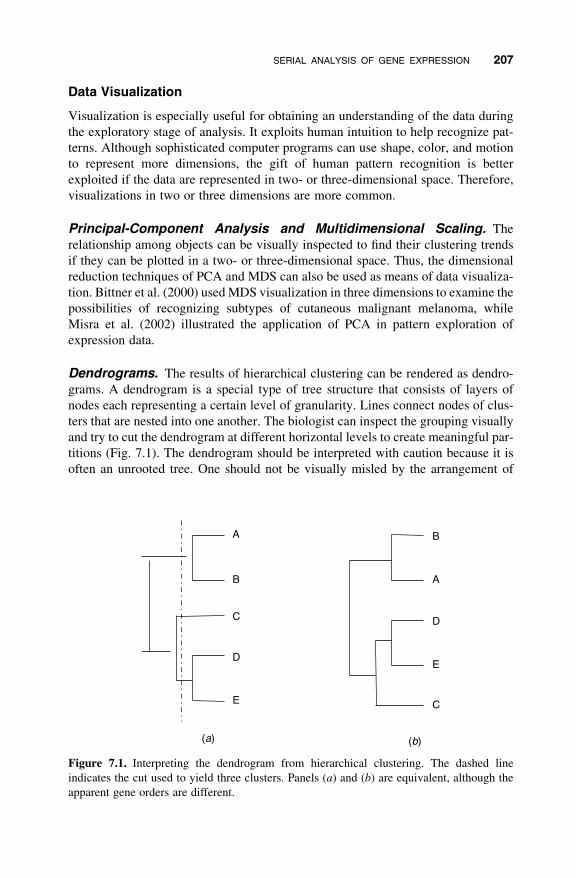
Dendrograms. The results of hierarchical clustering can be rendered as dendro-

grams. A dendrogram is a special type of tree structure that consists of layers of

nodes each representing a certain level of granularity. Lines connect nodes of clus-

ters that are nested into one another. The biologist can inspect the grouping visually

and try to cut the dendrogram at different horizontal levels to create meaningful par-

titions (Fig. 7.1). The dendrogram should be interpreted with caution because it is

often an unrooted tree. One should not be visually misled by the arrangement of

Figure 7.1. Interpreting the dendrogram from hierarchical clustering. The dashed line

indicates the cut used to yield three clusters. Panels (a) and (b) are equivalent, although the

apparent gene orders are different.


the objects in the dendrogram, since the branches at each node can be flipped. In

Figure 7.1, dendrograms (a) and (b) are exactly equivalent, although their orders

are completely different.

Data Matrix Visualization. The expression data matrix can be visualized as a

color map (each value encoded with a certain color). Eisen et al. (1998) combined

the color map with the dendrogram to help biologists rapidly assimilate and interpret

microarray data. Our discussion has focused on machine-learning approaches to

identify patterns. Here we briefly survey two other approaches to analysis of gene

expression data and provide examples of applications to biological problems.

Other Types of Gene Expression Data Analysis

Pattern Recognition. This type of analysis is usually applied to large collections

of patient samples (Perou et al., 2000) or to datasets collected by measuring

expression changes during a time course (Spellman et al., 1998) under numerous

perturbations (Hughes et al., 2000). Machine-learning methodologies, either super-

vised or unsupervised, are used to recognize patterns in these large datasets.

Detecting Differentially Expressed Genes. The goal of this type of analysis is

to statistically detect differentially expressed genes under predefined conditions or

treatments. Many criteria have been proposed for identifying significant changes.

Early rule-of-thumb methods only consider the expression differences by picking

genes with a change of more than twofold. A simple statistical model using

Student’s t-test or ANOVA can take the observed variations into account. However,

even when performed in triplicate, microarray experiments usually lack adequate

degrees of freedom to reliably estimate the true variance. Thus, modified t-tests

have been proposed either by using pooled sample variance estimations (Li et al.,

2001) or by regularization (Tusher et al., 2001). Bayesian approaches have also

been proposed (Baldi and Long, 2001; Lonnstedt and Speed, 2002). Generally,

these statistical methods use a gene-by-gene modeling approach, which necessitates

corrections for testing multiple comparisons. The utilization of standard Bonferroni

correction and Westfall–Young step-down p-value adjustments to control family-

wise error rate has been investigated (Dudoit et al., 2002), and others have argued

that a less conservative method to control false discovery rate is more appropriate

in the context of microarray analysis (Tusher et al., 2001).

Understanding Network Regulations. A third and more challenging approach

is to analyze expression data in the context of gene regulation networks. A major

characteristic of living organisms is that the expression levels of different genes

are interconnected with one another through complex regulatory networks and

pathways. Microarray data have been reexamined in the context of protein–protein

interaction networks (Ge et al., 2001), protein–DNA interaction networks (Aubrey

et al., 2001), and literature data-mining networks (Sluka, 2001). An even greater


challenge is to use gene expression data to elucidate the underlying blueprint of bio-

logical regulatory networks (Greller and Somogyi, 2002). Formal mathematical

tools such as Bayesian networks (Friedman et al., 2000), Bayesian decomposition

(Bidaut et al., 2001), and SVD (Yeung et al., 2002) have been applied to this

challenge, but successful application of this approach will require larger expression

datasets than are currently available.

Biological Applications of Expression Profiling

Microarray and SAGE-based expression profiling has been applied to a number of

biological problems.

Gene Annotation. The annotation of the human genomic sequence requires the

identification of all coding and noncoding exons. These exons can be computation-

ally predicted but must also be experimentally confirmed and assigned to their

respective genes. Using the idea that all exons of a given gene will be expressed

coordinately, Shoemaker et al. (2001) have placed all known or predicted exons

from chromosome 22 q on microarrays and conducted a series of hybridizations to

those chips. Genes with similar biological functions also tend to be coexpressed

under a variety of experimental conditions. This “guilt-by-association” approach

can be used to assign putative functions to uncharacterized genes that do not

share any sequence or structural similarity with known proteins. An unsupervised

learning approach to clustering was used to infer the function of uncharacterized

Saccharomyces and human genes in this way (Eisen et al., 1998). Support vector

machines have also been utilized to functionally classify genes in a supervised-

learning manner (Brown et al., 2000).

Elucidation of Transcriptional Control Pathways. SAGE analysis after

induction of p53 by heat shock (Madden et al., 1997) and microarray analysis

after zinc-induced p53 expression (Zhao et al., 2000) both identified hundreds of

genes whose expression levels are regulated by p53. These genes fell into categories

of apoptosis and growth arrest, cytoskeletal function, growth factors, extracellular

matrix, and adhesion proteins. These relatively simple experiments were able to

rapidly outline the entire regulatory pathway for this important protein. Similar

experiments demonstrated that BRCA1 stimulates the GADD45 and JNK/SAPK

apoptosis pathways (Harkin et al., 1999). Interestingly, these experiments have

shown that p53 and BRCA1 work together in a coordinated network. Methods

have been proposed to reverse engineer such transcription networks (D’Haeseleer

et al., 2000).

Identification of Transcription Factor Binding Sites. Sequences upstream

of yeast genes with similar expression profiles have been searched with pattern dis-

covery algorithms to identify conserved gene regulatory elements (Brazma et al.,

1998). This approach identified several known yeast transcription factor binding

sites. Novel targets for the yeast transcription factors SBF and MBF were identified


using an extension of this approach in which protein was chemically crosslinked to

DNA in vivo, purified by immunoprecipitation, PCR amplified, and then used to

probe microarrays (Iyer et al., 2001). This powerful approach identified over 200

novel gene targets for these transcription factors.

Cancer Research. Molecular classification of malignant tissue was discussed in

the introduction to this chapter. Other work has demonstrated that gene expression

patterns can be used to identify the tissue of origin of most tumors (Ross et al.,

2000). The CGAP has databased more than 100 SAGE libraries constructed from

normal and malignant tissue. Analysis of these data has identified hundreds of

genes involved in cancer pathogenesis, ranging from angiogenesis factors to cell

cycle regulators to transcription factors (Lal et al., 1999). The molecular pharma-

cology of cancer has been addressed by profiling gene expression of 60 cancer

cell lines before and after drug treatments. This work has led to methods for predict-

ing drug sensitivity to chemotherapeutic agents on the basis of gene expression

(Scherf et al., 2000). In a related study, chemoinformatics (high-throughput screen-

ing informed by crystal structures and bioinformatics) was used to develop kinase

inhibitors (Gray et al., 1998). The effects of these inhibitors were then characterized

by expression analysis before and after drug treatment.

Identifying and Prioritizing Candidate Genes for Complex GeneticDisorders. The techniques of gene expression profiling can assist in the search

for and analysis of candidate genes for complex genetic disease. Linkage analysis

(described in detail in Chapters 9–11) can identify genomic regions that harbor sus-

ceptibility loci for a complex disease; however, the regions of linkage are frequently

large (20 cM or greater) and may contain hundreds of genes. It is impractical or

impossible to evaluate all of these positional candidates for possible disease-related

polymorphisms, and prioritization of candidates solely on the basis of known or

inferred biological activity could miss many relevant genes.

Identifying and demonstrating the effects of polymorphisms in susceptibility

genes in complex disease can be challenging. While there exist rare premature

stop-codon mutations such as those in the TIGR/myocilin gene that lead directly

to glaucoma (Allingham et al., 1998; Suzuki et al., 1997), the more common situ-

ation is likely to be the identification of polymorphisms—defined as having .1%

frequency in the population—that increase risk of developing disease but may not

by themselves directly result in disease. This is the very nature of complex disease:

Multiple susceptibility genes will exist, with predisposing polymorphisms in any

one gene showing reduced penetrance as well as potential interactions with environ-

mental factors. Thus some individuals will have a given predisposing polymorphism

yet will not exhibit disease, while at the same time, other individuals that do exhibit

disease will lack that specific predisposing polymorphism. These difficulties in

the interpretation of polymorphisms or sequence variants reflect our evolving

understanding of the genetic etiology of complex diseases in general.

Precisely because of these difficulties, the experimental approaches with the

greatest likelihood of success will combine multiple different kinds of analysis,


including family-based linkage and association analysis, gene expression analysis,

and functional studies of normal and mutant proteins. This combination of strategies

takes advantage of the strengths of each method. Gene expression studies can benefit

the search for susceptibility loci in several ways.

Expression Profiling to Prioritize Candidate Genes. Linkage intervals har-

boring candidate genes can be quite large and encompass hundreds of genes. These

genes can be prioritized for mutation and polymorphism detection by using micro-

array or SAGE analysis on the relevant tissue. For example, the Udall Parkinson

Disease Center of Excellence at the Duke University Medical Center has conducted

SAGE and microarray analysis of substantia nigra tissue from Parkinson disease

(PD) patients and age-matched controls. The substantia nigra is a pivotal tissue in

PD—patients exhibit a dramatic loss of dopaminergic neurons in this tissue as

disease progresses. Genes whose expression levels are increased or decreased in

PD patients as compared to controls are good candidates for PD susceptibility

genes, as are genes that are preferentially expressed in the substantia nigra as com-

pared to other neural tissues. Hundreds of genes will be differentially expressed in

this way, but only a subset of these differentially expressed genes are located within

linkage intervals. These selected genes represent excellent candidates because two

independent experimental procedures (linkage mapping and expression profiling)

have identified them as potential susceptibility genes. In this way, expression analy-

sis can dramatically reduce the number of candidate genes that must be evaluated

following linkage analysis. This combined strategy has also been used to identify

a number of high-probability candidate genes for mania and psychosis (Niculescu

et al., 2000).

Annotation of Genes within Linkage Intervals. The SAGE approach dis-

cussed above will be especially powerful when combined with the recently devel-

oped “long SAGE” protocol (V. Velculescu, personal communication). This

modified SAGE protocol uses a different tagging enzyme to generate 20-bp

SAGE tags rather than the standard 14-bp tags. While this increases sequencing

costs, it greatly reduces redundancy in tag-to-gene mapping. Also, primers designed

from long SAGE tags can be used in conjunction with oligo dT primers to directly

amplify the 30 ends of novel genes from total RNA. Subsequent 50 or 30 rapid ampli-

fication of cDNA ends (RACE) allows the isolation of the full-length transcript.

Because SAGE is an open-platform technology (it does not rely on prior knowledge

of genes), this strategy will allow the identification of entirely novel genes within

linkage intervals.

Genes within a linkage interval can also be annotated by constructing a microar-

ray of all known or predicted exons within the interval. This is a large undertaking

but is becoming increasingly feasible as both genomic sequence quality and micro-

array spotting technologies improve. Such an array could then be probed with RNA

from the relevant tissue to determine the genes and exons expressed in that tissue.

This approach has been used to experimentally annotate the genes expressed on

22q (Shoemaker et al., 2001). Further, if RNA from an affected individual were


used to probe such an array, patient-specific defects in gene expression or transcript

splicing patterns could be detected directly. Such changes are often very difficult to

detect by searching for sequence variations in the genomic DNA of affected

individuals.

Gene expression profiling is an extraordinarily powerful research tool. We have

concentrated here on two techniques: SAGE and microarray hybridization. These

approaches have been used to characterize the regulation of transcription in many

organisms and systems, but their application to complex disease is still in its early

stages. We have described a few ways in which these techniques might be applied

to this area of research, and undoubtedly many more applications will follow as the

full potential of gene expression profiling is realized.

REFERENCES

Alizadeh AA, Eisen MB, Davis RE, Ma C, Lossos IS, Rosenwald A, Boldrick JC, et al (2000):

Distinct types of diffuse large B-cell lymphoma identified by gene expression profiling.

Nature 403:503–511.

Allingham RR, Wiggs JLdlPMA, Vollrath D, Tallett DA, Broomer R, Jones KH, Del Bono

EA, Kern J, Patterson K, Haines JL, and Pericak-Vance MA (1998): Gln368STOP myo-

cilin mutation in families with late-onset primary open-angle glaucoma. Invest Ophthal-

mol Vis Sci 39:2288–2295.

Alon U, Barkai N, Notterman DA, Gish K, Ybarra S, Mack D, Levine AJ (1999): Broad

patterns of gene expression revealed by clustering analysis of tumor and normal colon

tissues probed by oligonucleotide arrays. Proc Natl Acad Sci USA 96:6745–6750.

Alter O, Brown PO, Botstein D (2000): Singular value decomposition for genome-wide

expression data processing and modeling. Proc Natl Acad Sci USA 97:10101–10106.

Aubrey N, Devaux C, di Luccio E, Goyffon M, Rochat H, Billiald P (2001): Androctonus a,

biotin, immunoconjugate, single-chain a, fragment, and strep t: A recombinant scFv/streptavidin-binding peptide fusion protein for the quantitative determination of the

scorpion venom neua. Biol Chem 382:1621–1628.

Audic S, Claverie J-M (1997): The significance of digital gene expression profiles. Genome

Res 7:986–995.

Baldi P, Long AD (2001): A Bayesian framework for the analysis of microarray expression

data: Regularized t-test and statistical inferences of gene changes. Bioinformatics

17:509–519.

Bidaut G, Moloshok TD, Grant JD, Manion FJ, Ochs MF (2001): Bayesian decomposition

analysis of gene expression in yeast deletion mutants. In: Lin SM, Johnson KF, eds.

Methods of Microarray Data Analysis, Vol. II. Boston, MA: Kluwer Acadmeic Publishers.

Bittner M, Meltzer P, Chen Y, Jiang Y, Seftor E, Hendrix M, Radmacher M, et al (2000): Mol-

ecular classification of cutaneous malignant melanoma by gene expression profiling.

Nature 406:536–540.

Brar AK, Handwerger S, Kessler CA, Aronow BJ (2001): Gene induction and categorical

reprogramming during in vitro human endometrial fibroblast decidualization. Physiol

Genom 7:135–148.


Brazma A, Jonassen I, Vilo J, Ukkonen E (1998): Predicting gene regulatory elements in

silico on a genomic scale. Genome Res 8:1202–1215.

Breiman L (1984): Wadsworth Statistics/Probability Series. Belmont: Wadsworth Inter-

national Group.

Brown MP, Grundy WN, Lin D, Cristianini N, Sugnet CW, Furey TS, Ares M Jr, Haussler D

(2000): Knowledge-based analysis of microarray gene expression data by using support

vector machines. Proc Natl Acad Sci USA 97:262–267.

Burges CJC (1998): A tutorial on support vector machines for pattern recognition. Data

Mining and Knowledge Discovery 2:121–167.

Burges CJC, Burges CJC, Smola AJ (1999): Advances in Kernel Methods: Support Vector

Learning. Cambridge: MIT Press.

Cannon RL, Dave JV, Bezdek JC (1986): Efficient implement of the fuzzy C-means clustering

algorithms. Trans Pattern Anal Machine Intell 8:248–255.

Chu S, DeRisi J, Eisen M, Mulholland J, Botstein D, Brown PO, Herskowitz I (1998): The

transcriptional program of sporulation in budding yeast. Science 282:699–705.

Cristianini N, Shawe-Taylor J (2000): An Introduction to Support Vector Machines and Other

Kernel-Based Learning Methods. New York: Cambridge University Press.

D’Haeseleer P, Liang S, Somogyi R (2000): Genetic network inference: From co-expression

clustering to reverse engineering. Bioinformatics 16:707–726.

Datson NA, van der Perk-de Jong J, van den Berg MP, de Kloet ER, Vreugdenhil E (1999):

MicroSAGE: A modified procedure for serial analysis of gene expression in limited

amounts of tissue. Nucleic Acids Res 27:1300–1307.

Davies DL, Bouldin DW (1979): Cluster separation measure. IEEE Trans Pattern Anal

Machine Intell 1:224–227.

Dubitzky W, Granzow M, Berrar D (2000): Comparing symbolic and subsymbolic machine learn-

ing approaches to classification of cancer and gene identification. In: Lin SM, Johnson KF,

eds. Methods of Microarray Data Analysis, Vol. I. Boston, MA: Kluwer Academic.

Dudoit S, Yang YH, Callow MJ, Speed TP (2002): Statistical methods for identifying differ-

entially expressed genes in replicated cDNA microarray experiments. Statistica Sinica

12:111–139.

Durbin BP, Hardin JS, Hawkins DM, Rocke DM (2002): A variance-stabilizing transform-

ation for gene-expression microarray data. Bioinformatics 18(Suppl 1):S105–S110.

Efron B (1983): Estimating the error rate of prediction rule—Improvement on cross-

validation. J Am Statist Assoc 78:316–331.

Efron B, Halloran E, Holmes S (1996): Bootstrap confidence levels for phylogenetic trees.

Proc Natl Acad Sci USA 93:7085–7090.

Efron B, Tibshirani R (1993): An Introduction to the Bootstrap, 57th ed. New York: Chapman

& Hall.

Eisen MB, Spellman PT, Brown PO, Botstein D (1998): Cluster analysis and display of

genome-wide expression patterns. Proc Natl Acad Sci USA 95:14863–14868.

Ellis M, Davis N, Coop A, Liu M, Schumaker L, Lee RY, Srikanchana R, Russell CG,

Singh B, Miller WR, Stearns V, Pennanen M, Tsangaris T, Gallagher A, Liu A,

Zwart A, Hayes DF, Lippman ME, Wang Y, Clarke R (2002): Development and validation

of a method for using breast core needle biopsies for gene expression microarray analyses.

Clin Cancer Res 8:1155–1166.

REFERENCES 213

Felsenstein J (1985): Confidence-limits on phylogenies—An approach using the bootstrap.

Evolution 39:783–791.

Fitch WM, Margoliash E (1967): Construction of phylogenetic trees. Science 155:279–284.

Fowlkes EB, Gnanadesikan R, Kettenring JR (1987): Variable selection in clustering and

other contexts. In: Daniel C, Mallows CL, eds. Design, Data, and Analysis, 380th ed.

New York: John Wiley & Sons.

Friedman N, Linial M, Nachman I, Pe’er D (2000): Using Bayesian networks to analyze

expression data. J Comput Biol 7:601–620.

Furey TS, Cristianini N, Duffy N, Bednarski DW, Schummer M, Haussler D (2000): Support

vector machine classification and validation of cancer tissue samples using microarray

expression data. Bioinformatics 16:906–914.

Gasch AP, Eisen MB (2002): Exploring the conditional coregulation of yeast gene expression

through fuzzy k-means clustering. Genome Biol 3:RESEARCH0059.

Ge H, Liu Z, Church GM, Vidal M (2001): Correlation between transcriptome and interac-

tome mapping data from Saccharomyces cerevisiae. Nat Genet 29:482–486.

Getz G, Levine E, Domany E (2000): Coupled two-way clustering analysis of gene micro-

array data. Proc Natl Acad Sci USA 97:12079–12084.

Gower JC (1966): Some distance properties of latent root and vector methods used in

multivariate analysis. Biometrika 53:325–338.

Gray NS, Wodicka L, Thunnissen AM, Norman TC, Kwon S, Espinoza FH, Morgan DO,

Barnes G, LeClerc S, Meijer L, Kim SH, Lockhart DJ, Schultz PG (1998): Exploiting

chemical libraries, structure, and genomics in the search for kinase inhibitors. Science

281:533–538.

Green CD, Simons JF, Taillon BE, Lewin DA (2001): Open systems: panoramic views of

gene expression. J Immunol Methods 250:67–79.

Greller LD, Somogyi R (2002): Reverse engineers map the molecular switching yards. Trends

Biotechnol 20:445–447.

Harkin DP, Bean JM, Miklos D, Song YH, Truong VB, Englert C, Christians FC, Ellisen LW,

Maheswaran S, Oliner JD, Haber DA (1999): Induction of GADD45 and JNK/SAPK-

dependent apoptosis following inducible expression of BRCA1. Cell 97:575–586.

Hertz J, Krogh A, Palmer RG (1991): Introduction to the Theory of Neural Computation.

Santa Fe Institute Studies in the Sciences of Complexity. Lecture Notes, Vol. 1. Redwood

City: Addison-Wesley.

Hilsenbeck SG, Friedrichs WE, Schiff R, O’Connell P, Hansen RK, Osborne CK, Fuqua SA

(1999): Statistical analysis of array expression data as applied to the problem of tamoxifen

resistance. J Nat Cancer Inst 91:453–459.

Hoffmann R, Seidl T, Dugas M (2002): Profound effect of normalization on detection of dif-

ferentially expressed genes in oligonucleotide microarray data analysis. Genome Biol

3:RESEARCH0033.

Huber W, Von Heydebreck A, Sultmann H, Poustka A, Vingron M (2002): Variance stabil-

ization applied to microarray data calibration and to the quantification of differential

expression. Bioinformatics 18(Suppl 1):S96–S104.

Hubert L, Arabie P (1985): Comparing partitions. J Classification 2:193–218.

Hughes TR, Marton MJ, Jones AR, Roberts CJ, Stoughton R, Armour CD, Bennett HA,

Coffey E, Dai H, He YD, Kidd MJ, King AM, Meyer MR, Slade D, Lum PY, Stepaniants


SB, Shoemaker DD, Gachotte D, Chakraburtty K, Simon J, Bard M, Friend SH (2000):

Functional discovery via a compendium of expression profiles. Cell 102:109–126.

Ishida N, Hayashi K, Hoshijima M, Ogawa T, Koga S, Miyatake Y, Kumegawa M, Kimura T,

Takeya T (2002): Large scale gene expression analysis of osteoclastogenesis in vitro and

elucidation of NFAT2 as a key regulator. J Biol Chem 277:41147–41156.

Iyer VR, Horak CE, Scafe CS, Botstein D, Snyder M, Brown PO (2001): Genomic binding

sites of the yeast cell-cycle transcription factors SBF and MBF. Nature 409:533–538.

Jain AK, Chandrasekaran B (1982): In: Krishnaiah PR, Kanal LN, eds. Handbook of

Statistics, Vol. 2. Amsterdam: North-Holland.

Jolliffe IT (1986): Principal Components Analysis. New York: Springer-Verlag.

Kepler TB, Crosby L, Morgan KT (2002): Normalization and analysis of DNA microarray

data by self-consistency and local regression. Genome Biol 3:RESEARCH0037.

Kohonen T (1995): Self-Organizing Maps. New York: Springer-Berlin.

Kruskal J (1964): Multidimensional scaling by optimizing goodness to fit to nonmetric

hypothesis. Psychometrika 29:1–27.

Lal A, Lash AE, Altschul SF, Celculescu V, Zhang L, McLendon RE, Marra MA, Prange C,

Morin PJ, Polyak K, Papadopoulos N, Vogelstein B, Kinzler KW, Strausberg RL, Riggins GJ

(1999): A Public database for gene expression in human cancers. Cancer Res 59:5403–5407.

Lee SW, Tomasetto C, Sager R (1991): Positive selection of candidate tumor-suppressor

genes by subtractive hybridization. Proc Nat Acad Sci USA 88:2825–2829.

Li YJ, Zhang L, Speer MC, Martin ER (2001): Evaluation of current methods of testing differ-

ential gene expression and beyond. In: Lin SM, Johnson KF, eds. Methods of Microarray

Data Analysis, Vol. II. Boston, MA: Kluwer Academic.

Liang P, Pardee AB (1992): Differential display of eukaryotic messenger RNA by means of

the polymerase chain reaction. Science 257:967–971.

Lonnstedt I, Speed T (2002): Replicated microarray data. Statistica Sinica 12:31–46.

MacQueen J (1967): Some methods for classification and analysis of multivariate obser-

vations. In: Cam LL, Neyman J, eds. Proceedings of the Fifth Berkeley Symposium on

Mathematical Statistics and Probability, Vol. 1. University of California Press.

Madden SL, Galella EA, Zhu J, Bertelsen AH, Beaudry GA (1997): SAGE transcript profiles

for p53-dependent growth regulation. Oncogene 15:1079–1085.

Man MZ, Wang X, Wang Y (2000): POWER_SAGE: Comparing statistical tests for SAGE

experiments. Bioinformatics 16:953–959.

Margulies EH, Innis JW (2000): eSAGE: Managing and analysing data generated with serial

analysis of gene expression (SAGE). Bioinformatics 16:650–651.

Misra J, Schmitt W, Hwang D, Hsiao LL, Gullans S, Stephanopoulos G, Stephanopoulos G

(2002): Interactive exploration of microarray gene expression patterns in a reduced dimen-

sional space. Genome Res 12:1112–1120.

Neilson L, Andalibi A, Kang D, Coutifaris C, Strauss JF III, Stanton JL, Green DPL (2000):

Molecular phenotype of the human oocyte by PCR-SAGE. Genomics 63:13–24.

Niculescu AB III, Segal DS, Kuczenski R, Barrett T, Hauger RL, Kelsoe JR (2000): Identify-

ing a series of candidate genes for mania and psychosis: A convergent functional genomics

approach. Physiol Genomics 4:83–91.

Perou CM, Sorlie T, Eisen MB, van de RM, Jeffrey SS, Rees CA, Pollack JR, Ross DT,

Johnsen H, Akslen LA, Fluge O, Pergamenschikov A, Williams C, Zhu SX, Lonning PE,

REFERENCES 215

Borresen-Dale AL, Brown PO, Botstein D (2000): Molecular portraits of human breast

tumours. Nature 406:747–752.

Peters DG, Kassam AB, Yonas H, O’Hare EH, Ferrell RE, Brufsky AM (1999): Comprehen-

sive transcript analysis in small quantities of mRNA by SAGE-lite. Nucleic Acids Res

27:e39.

Quinlan JR (1996): Learning decision tree classifiers. ACM Comput Surv 28:71–72.

Raffelsberger W, Dembele D, Neubauer MG, Gottardis MM, Gronemeyer H (2002): Quality

indicators increase the reliability of microarray data. Genomics 80:385–394.

Ross DT, Scherf U, Eisen MB, Perou CM, Rees C, Spellman P, Iyer V, Jeffrey SS, van

de Rijn M, Waltham M, Pergamenschikov A, Lee JC, Lashkari D, Shalon D, Myers TG,

Weinstein JN, Botstein D, Brown PO (2000): Systematic variation in gene expression

patterns in human cancer cell lines [see comments]. Nat Genet 24:227–235.

Scherf U, Ross DT, Waltham M, Smith LH, Lee JK, Tanabe L, Kohn KW, Reinhold WC,

Myers TG, Andrews DT, Scudiero DA, Eisen MB, Sausville EA, Pommier Y, Botstein

D, Brown PO, Weinstein JN (2000): A gene expression database for the molecular

pharmacology of cancer. Nat Genet 24:236–244.

Schroeder SR, Oster-Granite ML, Berkson G, Bodfish JW, Breese GR, Cataldo MF, Cook EH,

et al (2001): Self-injurious behavior: Gene-brain-behavior relationships. Ment Retard Dev

Disabil Res Rev 7:3–12.

Shoemaker DD, Schadt EE, Armour CD, He YD, Garrett-Engele P, McDonagh PD,

Loerch PM, et al (2001): Experimental annotation of the human genome using microarray

technology. Nature 409:922–927.

Skinner HA (1978): Differentiating contribution of elevation, scatter and shape in profile

similarity. Ed Psychol Measur 38:297–308.

Sluka JP (2001): Extracting knowledge from genomic experiments by incorporating the bio-

medical literature. In: Lin SM, Johnson KF, eds. Methods of Microarray Data Analysis,

Vol. II. Boston, MA: Kluwer Academic.

Sneath PHA, Sokal RR (1973): Numerical Taxonomy; the Principles and Practice of Numeri-

cal Classification. San Francisco: W. H. Freeman.

Spellman PT, Sherlock G, Zhang MQ, Iyer VR, Anders K, Eisen MB, Brown PO, Botstein D,

Futcher B (1998): Comprehensive identification of cell cycle-regulated genes of the yeast

Saccharomyces cerevisiae by microarray hybridization. Mol Biol Cell 9:3273–3297.

Suzuki Y, Shirato S, Taniguchi F, Ohara K, Nishimaki K, Ohta S (1997): Mutations in the

TIGR gene in familial primary open-angle glaucoma in Japan. Am J Hum Genet

61:1202–1204.

Tamayo P, Slonim D, Mesirov J, Zhu Q, Kitareewan S, Dmitrovsky E, Lander ES, Golub TR

(1999): Interpreting patterns of gene expression with self-organizing maps: Methods and

application to hematopoietic differentiation. Proc Natl Acad Sci USA 96:2907–2912.

Tusher VG, Tibshirani R, Chu G (2001): Significance analysis of microarrays applied to the

ionizing radiation response. Proc Natl Acad Sci USA 98:5116–5121.

Valentini G (2002): Gene expression data analysis of human lymphoma using support vector

machines and output coding ensembles. Artif Intell Med 26:281–304.

Velculescu VE, Zhang L, Vogelstein B, Kinzler KW (1995): Serial analysis of gene

expression. Science 270:484–487.

Virlon B, Cheval L, Buhler JM, Billon E, Doucet A, Elalouf JM (1999): Serial microanalysis

of renal transcriptomes. Proc Natl Acad Sci USA 96:15286–15291.


Wang X, Ghosh S, Guo SW (2001): Quantitative quality control in microarray image proces-

sing and data acquisition. Nucleic Acids Res 29:e75.

Yang MC, Ruan QG, Yang JJ, Eckenrode S, Wu S, McIndoe RA, She JX (2001): A statistical

method for flagging weak spots improves normalization and ratio estimates in microarrays.

Physiol Genomics 7:45–53.

Yang YH, Dudoit S, Luu P, Lin DM, Peng V, Ngai J, Speed TP (2002): Normalization for

cDNA microarray data: A robust composite method addressing single and multiple slide

systematic variation. Nucleic Acids Res 30:e15.

Yeung MK, Tegner J, Collins JJ (2002): Reverse engineering gene networks using singular

value decomposition and robust regression. Proc Natl Acad Sci USA 99:6163–6168.

Zadeh LA (1965): Fuzzy sets. Information and Control 8:338–353.

Zhang K, Zhao H (2000): Assessing reliability of gene clusters from gene expression data.

Functional & Integrative Genomics 1:156–173.

Zhang L, Zhou W, Velculescu VE, Kern SE, Hruban RH, Hamilton ST, Vogelstein B, Kinzler

KW (1997): Gene expression profiles in normal and cancer cells. Science 276:1268–1272.

Zhao R, Gish K, Murphy M, Yin Y, Notterman D, Hoffman WH, Tom E, Mack DH,

Levine AJ (2000): Analysis of p53-regulated gene expression patterns using oligo-

nucleotide arrays. Genes Dev 14:981–993.

REFERENCES 217

Documents

Genetic Analysis of Complex Diseases || Data Analysis Issues in Expression Profiling