Embed Size (px)
Citation preview
GeneraIized Least Squares F-Test and Relevant ML Estimation in Regression Analysis
With Two-Stage Cluster Samples
by S R Paul
Dept ofMathematics amp Statistics WMSR96-01
May 1996
Generalized Least Squares F-Test and Relevant
ML Estimation in Regression Analysis
With Two-Stage Cluster Samples
S R Paul
For regression analysis of data from two-stage duster sampling we extend the GLS
F-test of Rao Sutradhar and Vue (1993) to the general situation in which the intracluster
correlations and the variances are possibly different The situations in which (i) the
variances are common and the intracluster correlations are possibly different and (ii) the
intracluster correlations and the variances are both common are dealt with as special
cases For all the models considered we derive the required transformed variables with
iid errors and the maximum likelihood estimates of the unknown intracluster correlations
Results of a small scale simulation study similar to that of Rao et al (1993) show that
the GLS F-test using maximum likelihood estimates of the intracluster correlations might
produce correct type I error rate irrespective of the amount of collinearity and intracluster
correlation
Keywords Equal and unequal intracluster correlations equal and unequal sample sizes
GLS F test maximum likelihood estimation size and power two-stage sampling
1 Introduction
The use of the standard F test in regression analysis of complex survey data leads to
inflated type I error rate (size) due to correlated errors in regression model appropriate for
clustered data In case of two-stage cluster samples Wu Holt and Holmes (1988) propose
a simple correction to the standard F-test which ~akes account of possible common or
heterogeneous intracluster correlations However for common intraclass correlation p they
SR Paul is Professor Department of Mathematics and Statistics University of Windsor Windsor Ontario Canada N9B 3P4 The author thanks JNK Rao for supplying details of simulation study in Rae et al (1993) and Brajendra C Sutradhar for several discussions during the earLy development of this paper
Typeset by AAAS-lEX
show by simulation that the corrected F-test performs much better than the standard Fshy
test in controlling the size for a scalar hpothesis It performs almost as well as the iterative
generalized least square (IGL8) F-test for large values of p and better than the IGL8 for
small p in controlling size Rao 8utradhar and Vue (1993) propose a simple GLS F test
which also takes account of common intracluster correlation and show also by simulation
that for both scalar and vector hypotheses the GLS F test performs as well as the corrected
F-test in controlling the size even for small p and that it leads to significant power gains
for large values of p
For the estimation of the common intra-cluster correlation p Wu et a1 (1988) use a two
step procedure and Rao et a1 (1993) use a method of fitting constants due to Henderson
(1953) Rao et a1 (1993) comment that the performance of the GLS F test using the
estimate of the common p by the two-step procedure of Wu et a1 (1988) is similar to
that of the GLS F test using the estimate of p by the method of fitting constants due to
Henderson (1953) These estimates however are method of moment type estimates and
they use data under the alternative hypothesis A disadvantage of the corrected F-test and
GLS test using such as estimate of p is that they produce inflated type I error rate with
increasing collinearity and large p (see Wu et a1 1988) A more appropriate approach
would be to esimate p using data under the null hypothesis Such an approach is taken in
the well-known score test (Rao 1947) or the C(a) test of Neyman (1959) However the
method of moment estimate of p such as that obtained by Hendersons procedure can not
be obtained under all null hypothesis situations We propose using maximum likelihood
estimates
Note that the GLS F-test proposed by Rao et a1 (1993) with common intracluster corshy
relation and variance is based on transformed data following Fuller and Battese (1973)
with iid errors In this paper we extend the GLS F-test to the general situation in which
the intracluster correaltions and the variances are possibly different The situations in
which (i) the variances are common and the intracluster correlations are possibly different
2
and (ii) the intracluster correlations and the variances are both common are dealt with as
special cases For all the models considered we derive the required transformed variables
with iid errors and the maximum likelihood estimates of the unknown intracluster correshy
lations The regression model and the associated GLS F test are given in section 2 In
section 3 we deal with the model and its variants the transformations and the maximum
likelihood estimation of the intracluster correlation(s A small scale simulation study
similar to that of Rao et al (1993) is given in section 4 to show the possible advantage of
using the maximum likelihood estimates of the intracluster correlations
2 The Regression Model and The GLS F Test
Following Fuller and Battese (1973) we consider a regression model with nested error
structure that allows for intracluster correlations
y = XfJ + c (21)
where X is an (n x k) matrix ofregression variables fJ is a vector of k regression parameters
E(c) = 0 and E(cc = D where D is positive definite The generalized least-squares
estimator of fJ is
which has cov (ffi) (XD-1X-lXD-1X Fuller and Battese (1973) show that if a
transformation matrix T can be found such that the transformed errors
euro = Tc
are uncorrelated with constant variances the generalized least-squares estimator fJ is
given by the ordinary regression of the transformed dependent variable y = Ty on the
transformed independent variable X = T X Thus for testing the vector hypothesis
Ho 0 fJ = b where 0 is a known q x k matrix of rank q( lt k) and b is a known q x 1
vector the standard F test based on the transformed data is based on
(OfJ - b) (X~X~rl (OfJ - b) qFGLS= ~~--~~~--~--~~--~~
(y - XJ) (y - Xf3) (n - k)
3
2
which has an exact F distribution with q and n k degrees of freedom where f3 =
(X X)-l Xy is the ordinary least squares estimator of f3 under the transformed model
and X~ = X (XX)-l C
We will see later that the regression model involves the variance components at or a or
the intracluster correlations Pi or p The F-distribution of the statistic FGLS is based on
the intracluster correlation parameter Pi or P and the variance parameter at or a2 being
known In practice these parameters are unknown If the parameters are replaced by some
consistent estimators the distribution of FGLS will be approximately correct For model
III Rao et al (1993)proposed estimating P by a moment type procedure due to Henderson
(1953) and Fuller and Battese (1973) which is consistent This procedure uses all data
under the full model ie under the alternative hypothesis In this paper we propose to
use instead maximum likelihood estimates of the variance and intracluster correlation
parameters under the null hypothesis
3 The Model Its Variants The Transformations
and Relevant Maximum Likelihood Estimation
31 The Model and its Variants
Consider a two stage cluster sample of n observaLions with c clusters at the first stage
of sampling and mi elements drawn from the ith-sampled cluster at the second stage
n = ~mi The model with the nested error structure is
(31)
and
where Yij is the response ofthejth element in the ith cluster Xij = (XijOXijl Xijk-r)
with XijO = 1 f3 = (f3o i3I f3k-I) is the vector of regression parameters Vi rv N (0 a~i)
and Uij rv N (0 a~i) Now denote al a~i + a~~ and Pi = a~dal Clearly Pi is the
4
intracluster correlation within the second stage units of the ith cluster Thus for two stage
cluster samples model (31) can be written as
Model I Y X3+E E N(O D)
I)( (X~Imiddot IX~) with Xi deshy0 bullwhere Y = Ylmiddotmiddotmiddot Yimiddotmiddotmiddot Ye Yi
noting the mi X k matrix with rows X~j j = 10 mi E = (E~middotmiddot E~middotmiddotmiddot E~) Ei
( Eil bull Eim D has a diagonal form Efo-Vi with Vi = (1 - Pi) Im- + PiJm- where Ip iso
bull )
1 bullbull
the p x p identity matrix and Jp is the p x p unit matrix
Different variants of model I are possible and have been dealt with by other authors
When 0 = u 2 for all i model I is identical to model (22) of Wu Holt and Holmes (1988)
which we write as
Model II y=X3+E E N (0 D)
2where D = u 2 Ef Vi and Y X 3 E and Vi are all same as those of model When uf u1
and Pi = P for all i model I is identical to the model dealt with by Campbell (1977) Scott
and Holt (1982) Rao Sutradhar and Vue (1993) We write this model as
Model III Y X3+E E N (OD)
where D u 2 EfWi and y X 3 and E are the same as those of model I and Wi = (1 shy1
P)lmi + pJmi middot
32 Transformations
The covariance matrix for the error vector E in model I is the block diagonal matrix
e h 2 _1 e _1 - _ -1 -~ D = (JjD i were Di Ui Vi Then D 2 = (JjD 2 where D - U i Vi Now Vi1 middot1middotmiddot
(1 - Pi)lmi + PiJmi which can be written as
where ti = 1 + (mi I)Pi Then it is easily verified that (see FUller and Battese 1973)
5
and euroi = (1Oi)Vi-euroi are uncorrelated with constant variances 1 Thus the matrix
Ti = (1OdVi- = 1 I lmi - I - [(l~Pd] i transforms the error vector euroUi(l-pd
to a vector of uncorrelated random variables with constant variances 1 Thus the transshy
formations for y and X are
yii = 1 (Yii - OiYiO) and xii = I (xii - OiXiO) Oi (1 - Pi) Oi (1 - Pi)
where 0i = 1- [(1- Pi) I + (mi -1) Pi] fho = ElYiimi andxiQ = E71xiimi
The transformed model can be written as yii = xij3 +uii j 1 mi i = 1 C or c
in matrix notation as Y= X3 + u where uii N(OI)or u N(O E9lm J SimilarlyIV
1
mit can be shown that for model II the matrix Ti = I [lmi - I - [(l~Pi)] J 1u(l-Pi) m transforms the error vector to to a vector of uncorrelated random variables with constant
variances 1 The transformation for y and X are
yij = 1 1 (Yij - OiYiO) and xii = 1 1 (Xij - OiXiO) O(I-Pi)2 O(I-Pi)2
where 0i = 1- [(1- Pi)1 I +(mi -1)pl ~ The transformed model then is Yij = Xij3 +uii
j = 1 mi i = 1 C where uii N(OI)or in matrix notation y = X3+u where c
u N(O E9Im) Finally for model III the transformation 1
Ti = Imi - I - [(1 - p) I + (mi-I) P ] i transforms the error vector euro to a vector of uncorrelated random variables with constant
variance 0 = 02(1- p) Clearly for model III the transformation for y and X are yij
Yii - OiYiO and xij = Xij - 0iXiQ where 0 = 1- [(1- p) I I + (mi -1)p] t The transformed
fI+ 1 modle IS Yij = Xijl- Uij J = mi t 1 c or in matrix notation Y = X 3 + u
where uij N(OO~) or u N(Oq~In)(See also Roo et al (1993))
34 Maximum Likelihood Estimates of Intraclass Correlation
We consider estimating the intracluster correlation parameters in presence of the reshy
gression parameters under the null hypothesis H0 C3 = b We assume that C i3 = b is
6
a consistent set of equations Then under the null hypothesis we will have k q regresshy
sion parameters Let 8 =(80 81 8k-l-q) be the vector of regression parameters to be
estimated under the null hypothesis and Zij =(ZijO Zij1 Zijk-l-qf be the vector of
covariates corresponding to the parameters 8 Note that the regression variables as well
as the dependent variable will be defined depending on the composition of C and b We
give a few examples from Graybill (1976 p 184) First we define the dependent variable
as s Suppose under the alternative hypothesis we have 4 regression variables X 1 X2 X 3
and X4
Example 1 If C = (01 -100) b = 0 that is Ho 31 = 32 then S y Zo = Xo = 1
ZI XI + X 2 Z2 = X3 Z3 = Xl and 8 = (80818283)
Example 2 If
C 0 1 -1 0 0) b (00)( o 0 0 1 -1 bull
that is Ho 31 = 32 and 33 = 34 then s = y Zo = Xo = 1 ZI = XI + X2 Z2 X3 + X4
and 8 = (808182)
Example 3 If o
C 1
1
that is Ho 31 = 32 = 33 = 34 then s y Zo = Xo 1 ZI = (X 1 + X2 + X3 + X4) and
8 = (808d
Example 4 If
= (0 1 -2 -4 0)C o 1 2 0 0
that is Ho 31 - 232 = 433 and 31 +232 6 then s = y - 6X 1 ~X3 Zl = X2 - 2X1 - X3
Z2 = X 4 and 8 = (8081 82) Note in this example this is not the only way we can define
J
Now under the null hypothesis model (31) reduces to Sij z~j8 + Vi + Uij ) =
1 mii 1C Further let Si = (Sil Simi) Zi = (Zitmiddot Zim) ti 1+
7
(mi - l)pi and di 1 + (mi -1)p Then OJ is the inverse of Vi with (ti - Pi)(1 - Pi)td
in the diagonal and -pi(I - Pi)ti everywhere else and 6i is the inverse of Wi with
(d i - p)(1 - p)di in the diagonal and -pl(I- p)di everywhere else
Now following Paul (1990) the estimating equation for Pi of model I is
where p ( - =1_1 1) bull S S = j~1 (j - j5)2
and SST = L~1 (j - jb)r5
(~ z0) -1~ 0 Once the es timale of p of p is obtained the estimate of q 1 is
amp~ _1 (SS- - p-SSTIt-)t mi t t t
Again the estimating equation for Pi of model II is
n1 - Pi)--1[SSi - SSTi1 + (mi - l)pnlttl ( 1)1 0 c - Pimi m1 - ti = (33)
2(1- Pi)-1(SSi - PiSSTlti) i=1
1where PiE ( - mi _ 1 1) and SSi and SSTi are the same as in equation (32) Once the c
estimate Pi of Pi is obtained the estimate of (12 is 2 = ~ 2(1- Pi)-1(SSi - PiSSTiti) i=1
Finally the estimating equation for P of model III is
where p 9 (- =1_1 1) SS = ~ (Sj - j6)2 and SST = 2( (j j6) 6 =
(2i Z6iZi) -1 (2i Z~6iSi) The estimate of (12 is not required here
4 Simulations
For ease of comparison the simulation design the regression model and the parameter
values considered here are the same as those considered by Rao et a1 (1993) and Wu et
a1 (1988) However for completeness we describe these in what follows
8
We consider the nested error regression model with two covariates xl= x and X2 Z
and equal mi m)
I c (41 )
Values of (Xij) Zij) were generated from the bivariate normal distribution with additional
random effects components to allow for intracluster correlations pz and Pz on both x and
Z
(42)
iid N (0 2) iid N (0 2) iiA N (0 2) iid N (0 2)wereh vxi Uux Vzi Uuz Uxij Uux uzij u uz Px
22 d _22 h 2_2+2 d 2 uux Ux an pz - uuz u z were Ux - uux uux an u z
are correlated with covariance u uxz and Uxij and Uzij are correlated with covariance u uxz
Also let pzz = uuxzuxuz and corr (xz) = uxzuxUZ) where Uxz = Uvzz + Uuzz and corr
(xz) denotes the correlation between Xij and Zij The parameters u~x UUXZ) u~z Uuxz etc
were chosen to satisfy u 20 Px 01 pz 05 Pzx 0 and corrx z) = -033
0 033 66 88
We first generated (Vzi Vzi) from bivariate normal distribution with mean vector 0
variances u~X) U~ZI and covariance Uvxz Next we generate m = 10 independent pairs
(Uzij Uzij) j 1 m from bivariate normal distribution with mean vector (00) varishy
ances u~x u~z and covariance Uuxz The pairs (Xij Zij) j = 1 m were then obtained
from (42) using JLx = 100 and JL = 200 This three-steps procedure was repeated 10 times
to generate 10 pairs (xz) from each of c = 10 clusters
We next turn to the generation of Yij for given (Xij Zij) fJo = 10 and (fJl fJ2) combinashy
tions given in Tables 1-2 For u 2 = 10 and selected p given in Tables 1-2 (or equivalently
u and u) we generated Vi id N(O u~) and Uij id N(O u) independently and then
obtain Yijfrom (41) The simulated data (Yij Xij Zij) j = 1 m i = 1 c were
used to compute the test statistics The simulations of YiS were repeated 10000 times
for each set of (xz) values in order to obtain estimates of actual type I error rate (size)
and power of each test statistic
9
We considered the hypothesis PI = P2 = 0 as reported by Rao et a1 (1993) Table
1 gives size estimates of the statistics FCLS(P) and FGLS(P) using Hendersons estimate
of p and the maximum likelihood estimate of p respectively There is evidence from the
simulation that FGLS(P) gives inflated type I error rate as the corr(xz) and p increase
The statistic FGLS(P) seems to control type I error rate adequately Table 2 gives power
estimates of the two statistics Power estimates of Fcns(P) are in general larger than those
of FCLS(fi) This is because the corresponding sizes are larger
Thus the statistics FCLS with maximum likelihood estimates of the unknown intraclusshy
ter correlations might produce correct type I error rate However we do not claim any
power advantage of FGLS(P)
References
Campbell C (1977) Properties of Ordinary and Weighted least squares Estimators for
Two-Stage Samples in Proceedings of the Social Statistics Section American Statisshy
tical Association 800-805
Fuller WA and Battese GE (1973) Transformations for Estimation of Linear Models
with Nested Error Structures Journal of the American Statistical Association 68
626-632
Graybill FA (1983) Theory and Application of the Linear Model Massachusetts Wadsworth
Henderson CR (1953) Estimation of Variance and Covariance Components Biometshy
rics 9 226-252
Neyman J (1959) Optimal asymptotic tests of composite hypothesis In Probability and
Statistics The Harold Cramer Volume U Grenarder (ed) New York John Wiley
Paul SR (1990) Maximum Likelihood Estimation of Intraclass Correlation in the Analshy
ysis of Familial Data Estimating Equation Approach Biometrika 77 549-555
Rao C R (1947) Large Sample Tests of Statistieal Hypothesis concerning several pashy
rameters with applications to problems of Estimation Proceedings of the Cambridge
10
Philosophical Society 44 50-57
Rao JNK Sutradhar BC and Yue K (1993) Generalized Least Squares F test in Reshy
gression Analysis with two-stage Cluster Samples Journal of the A merican Statistical
Association 88 1388-139l
Scott AJ and Holt D (1982) The Effect of Two-Stage Sampling on Ordinary Least
Squares Methods Journal of the American Statistical Association 77 848-854
Wu CFJ Holt D and Holmes DJ (1988) The Effect of Two-Stage Sampling on the
F Statistics Journal of the Americal Statistical Assocation 83 150-159
11
Table 1 Size Estimates () of FGu(i)) and FGpounds(~) Tests of Ho
PI =0 P1 =0 ex = OS and 1
bull =OS bull = 10
Corr(xz) p FGLSO) FGu(l ) FGu(p) FGu(fJ )
-33
0 05 1 3 5
51 58 62 61 58
43 47 49 50 51
96 111 117 117 111
89 96 98 103 101
0
0 05 1 3 5
51 58 61 59 57
44 49 50 51 51
97 109 115 112 109
90 96 99 100 101
33
0 05 1 3 5
49 59 63 61 58
42 49 51 51 51
95 113 117 118 111
88 97 99 102 102
66
0 05 1 3 5
43 59 68 76 73
35 43 48 51 53
89 115 125 133 131
81 97 103 108 106
88
0 05 10 30 50
43 60 69 75 75
35 43 48 49 50
88 114 123 132 129
81 95 101 107 105
Table 2 Power Estimates () of FGu(p) and FGLSlaquo(J) Tests of No Pl = 0 and P =0 CI =051 vs Specified Alternatives
With c=lO m=1O and corr(xz)= 0 33bull66
CI =05 CI =1
PI P p FGu(p) FGu(p) FGLS(p) FGu(P)
corr(xz)=O
1 1
0 05 10 30 50
382 382 380 417 521
359 354 353 396 505
517 509 506 545 646
498 483 480 526 631
2bull2
0 05 10 30 50
926 919 917 947 983
917 906 905 939 980
961 954 955 971 993
958 948 947 966 992
corr(xz)=33
1 1
0 05 10 30 50
502 499 502 561 685
481 472 478 539 671
621 621 624 675 794
609 601 601 659 783
2 bull 2
0 05 10 30 50
978 975 975 990 998
975 971 970 988 998
990 988 989 995 999
989 987 986 995 999
corr(xz)=66
1 1
0 05 10 30 50
590 601 608 683 813
576 563 590 665 801
707 711 722 786 886
700 699 705 776 879
2bull2
0 05 10 30 50
993 993 994 998 100
993 993 993 997 100
998 998 998 999 100
998 998 997 999 100
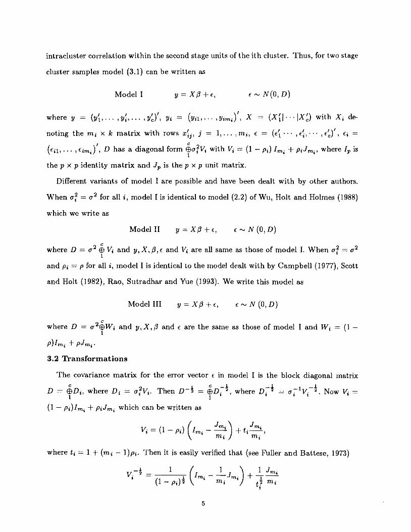
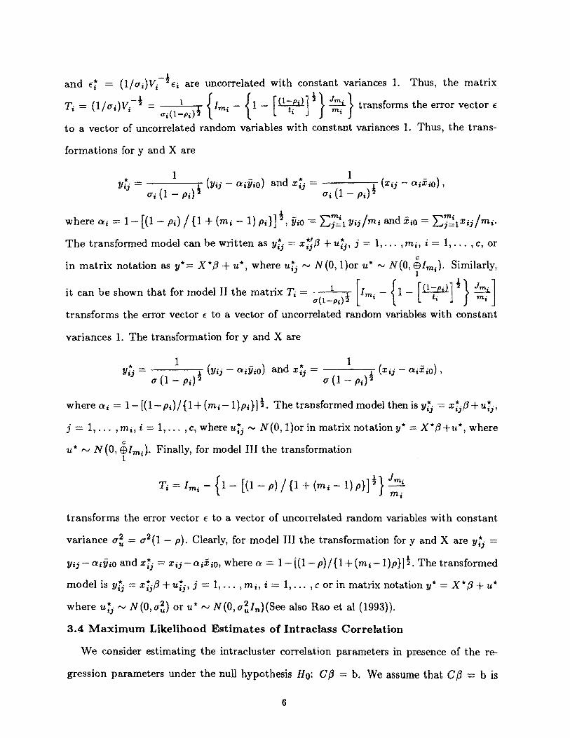
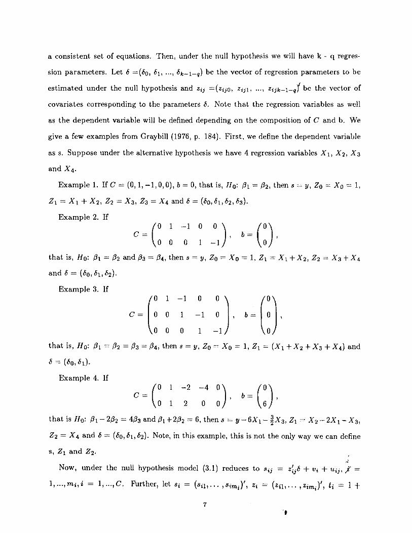
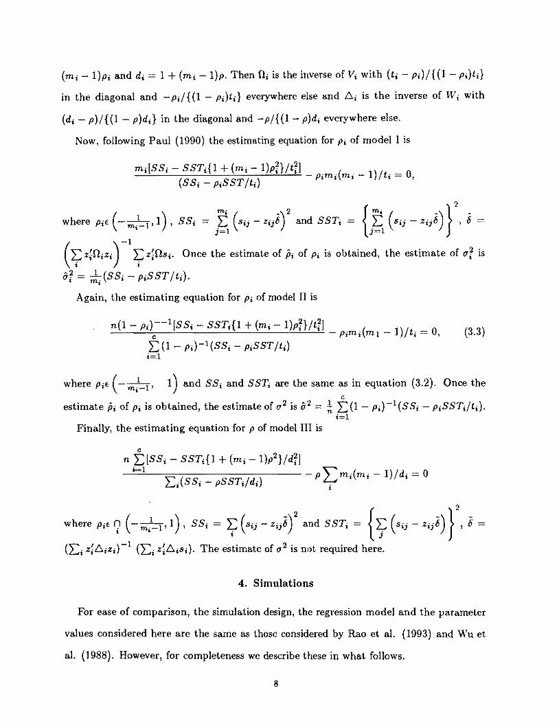
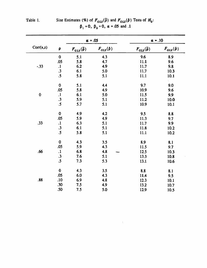
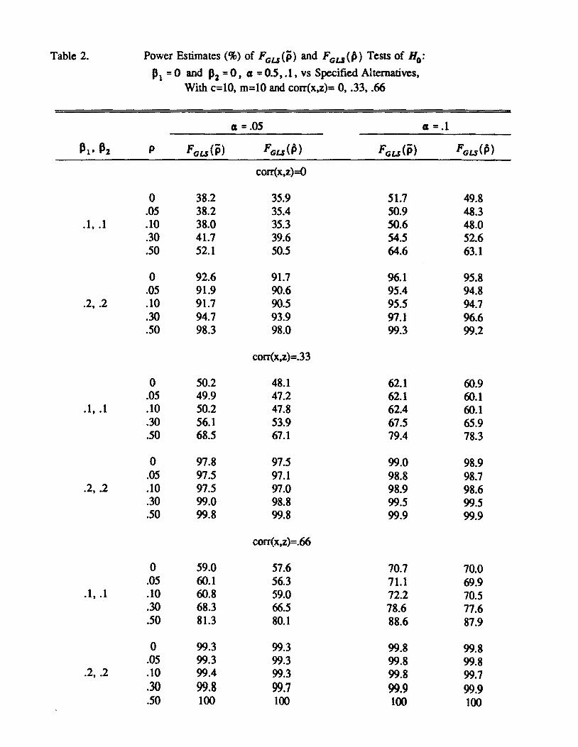