GENERALIZED LEAST SQUARES INFERENCE IN PANEL AND

MULTILEVEL MODELS WITH SERIAL CORRELATION AND FIXED

EFFECTS

CHRISTIAN B. HANSEN†

Abstract. In this paper, I consider generalized least squares (GLS) estimation in fixed

effects panel and multilevel models with autocorrelation. A complication which arises in

implementing GLS estimation in these settings is that standard estimators of the covariance

parameters necessary for obtaining the feasible GLS estimates will typically be inconsistent

due to the inclusion of individual specific fixed effects. Focusing on the case where the

disturbances follow an AR(p) process, I offer a bias-correction for the AR coefficients which

is simple to implement and will be valid in the presence of fixed effects and individual

specific time trends. I develop asymptotic properties of the bias-corrected estimator as

the cross-section dimension goes to infinity with the time dimension fixed and as both the

cross-section and time series become large. I also present asymptotic properties of the

feasible GLS estimator in both asymptotics and derive the higher order bias and variance

of the feasible GLS estimator in the second case. The usefulness of GLS and the derived

bias-correction for the parameters of the autoregressive process is illustrated through a

simulation study which uses data from the Current Population Survey Merged Outgoing

Rotation Group files.

Keywords: panel, multilevel, autocorrelation, generalized least squares, higher-order,

bias-correction

JEL Codes: C12, C13, C23

Date: 14 March 2003. This draft: 13 July 2004.

I would like to thank Josh Angrist, Jim Poterba, Byron Lutz, Joanna Lahey, and David Lyle as well

as seminar participants at Brigham Young University, the University of Chicago, Boston University, Brown

University, the University of Michigan, the University of Illinois, and Stanford University for helpful com-

ments and suggestions. I am especially grateful to my advisors, Whitney Newey and Victor Chernozhukov,

for comments, suggestions, and support provided throughout the development of this paper. All remaining

errors are mine. † University of Chicago, Graduate School of Business, 1101 East 58th Street, Chicago, IL

60637. Email: chansen1@gsb.uchicago.edu.

1

1. Introduction

Many economic analyses are characterized by regressions involving both aggregate and

individual level data, that is, multilevel data. This is especially prevalent in differences-

in-differences (DD) estimation, and policy analysis more generally, where the dependent

variable is often an individual level outcome and the covariate of interest is a policy which

applies to all individuals within a group. For example, in a study of the impact of the

minimum wage on employment, the dependent variable may be the employment in a firm

in group s at time t, and the policy would be the minimum wage in group s at time

t. While this sampling design does not pose any serious problems for estimation of the

linear model, it may lead to serious problems for inference. In particular, the sampling

design gives rise to potential sources of correlation between observations, termed here the

“clustering problem” and the “policy autocorrelation problem”, that would be ignored in

computing conventional least squares standard errors. The clustering problem is caused by

the presence of a common unobserved random shock at the group level that will lead to

correlation between all observations within each group. The policy autocorrelation problem

arises if the groups (not necessarily the individuals within the groups) are followed over

time and the group level shocks are serially correlated, which will result in correlation

between individuals from the same group at different time periods.1 In general, ignoring

these correlations will bias conventional least squares standard errors and lead to misleading

inference. The purpose of this paper is to provide accurate, powerful, and easily computable

inference methods for data which are potentially affected by both the clustering problem

and the policy autocorrelation problem.

The clustering problem has long been recognized in the econometric literature on panel

data, and has more recently been emphasized in economics in other contexts which involve

multi-stage sampling or multilevel data. There are a number of methods for dealing with

this problem which are available in most statistical packages. The most common approach is

to estimate a linear model with OLS and then correct the standard errors for the intracluster

correlation as in Moulton (1986), Arellano (1987), or Kezdi (2002). Feasible Generalized

Least Squares (FGLS)2 estimation may also be performed easily and will asymptotically

result in a more efficient estimator and more powerful tests than OLS.

The policy autocorrelation problem has received considerably less attention from applied

economic researchers. In a survey of DD papers published in six leading applied economics

1For simplicity, I will typically refer to time periods as years.2Throughout, I refer to GLS as the infeasible estimator which assumes that the variance matrix of the

disturbances is known and to FGLS as a feasible estimator which uses estimates of the elements of the

variance matrix.

2

journals from 1990-2000,3 Bertrand, Duflo, and Mullainathan (2004) found that only five

of 65 articles with a potential serial correlation problem explicitly address it; and in sim-

ulations based on individual level Current Population Survey Merged Outgoing Rotation

Group (CPS-MORG) data, they found a 44% rejection rate for a 5% level test using stan-

dard techniques which correct only for the intragroup correlation. To focus on the policy

autocorrelation problem, they also performed a simulation based on data from the CPS-

MORG aggregated to the group-year level. In the aggregate data, they found that using

simple parametric models for the serial correlation did not correct the size distortion, but

that tests based on the OLS estimator which flexibly account for serial correlation, such

as the bootstrap or using a variance matrix robust to arbitrary correlation at the group

instead of the group-year level, had approximately correct size. However, while these tests

appear to have correct size, the results of Bertrand, Duflo, and Mullainathan (2004) also

suggest that they have low power against relevant alternatives.

In this paper, I contribute to the existing literature by offering computationally attrac-

tive FGLS-based estimation and inference procedures that deliver accurate and powerful

inference in settings that are subject to both the clustering problem and the policy au-

tocorrelation problem. In particular, I explicitly consider FGLS estimation in a general

model for grouped individual and aggregate level data which incorporates standard DD

and panel models and could easily be extended to cases with additional levels of variation.

I present an aggregation strategy building upon Amemiya (1978) which recovers the FGLS

estimates and is computationally convenient in large data sets. I then focus on estimation

and inference under the assumption that the group-year shock follows a stationary AR(p)

process. FGLS estimation and inference based on parametric time series models for the

error process is complicated by the relatively short time dimension available in many policy

analyses and the inclusion of group-level fixed effects. It is well-known that estimates of

the parameters of time series models in panel data with fixed effects are biased when the

time dimension is short due to the incidental parameters problem. Using a strategy due to

Nickell (1981) and Solon (1984), I derive a bias correction for the coefficients of an AR(p)

model. I then develop asymptotic inference results for the bias-corrected coefficients and

the corresponding FGLS estimator which cover both conventional panel asymptotics where

the number of groups goes to infinity with the time dimension fixed and asymptotics where

the number of groups and time periods go to infinity jointly as in Phillips and Moon (1999),

Hahn and Kuersteiner (2002), and Hahn and Newey (2002). I also consider higher-order

properties of the FGLS estimator in asymptotics where the number of groups and time pe-

riods go to infinity jointly showing that, while FGLS estimates based on both conventional

and bias-corrected estimates of the AR parameters are first-order asymptotically equivalent

to GLS, there are higher-order efficiency gains to using bias-corrected AR parameters. The

3The journals are The American Economic Review, Industrial and Labor Relations Review, The Journal

of Labor Economics, The Journal of Political Economy, The Journal of Public Economics, and The Quarterly

Journal of Economics.

3

usefulness of the bias correction and the FGLS procedure are then demonstrated through

a simulation study based on the CPS-MORG.

The results from the simulation study strongly support the use of the FGLS procedure

with bias-corrected AR coefficients for performing inference in settings with combined indi-

vidual and grouped data where the groups are potentially autocorrelated. As in Bertrand,

Duflo, and Mullainathan (2004), I find that conventional OLS and, to a lesser extent, conven-

tional FGLS suffer from severe size distortions in the presence of the policy autocorrelation

and clustering problems. This size distortion is essentially removed by OLS with standard

errors clustered by group and the bias-corrected FGLS procedure. However, the FGLS pro-

cedure clearly dominates OLS with standard errors robust to arbitraty correlation within

groups in terms of both power and confidence interval length. For example, in a simulation

performed by resampling directly from the CPS-MORG, I find that conventional OLS has

a rejection rate of 37% for a 5% level test. In contrast, OLS with standard errors clustered

by group rejects 6.6% of the time, and FGLS based on bias-corrected AR(3) coefficients

has a 6.4% rejection rate. At the same time, the power of the bias-corrected FGLS-based

procedure versus the alternative that the treatment increases the dependent variable by 2%

is 0.788 compared to 0.344 from OLS with clustered standard errors. Similarly, the length

of the FGLS confidence interval is 0.028 compared to the OLS interval length of 0.050.

The remainder of this paper is organized as follows. In Section 2, I briefly review GLS

estimation in settings involving both individual and aggregate data and present a compu-

tationally attractive procedure for obtaining the GLS estimates which will be valid as the

group size grows large within each group-year cell. Section 3 presents a bias-correction

for fixed effects estimates of the parameters of a pth order autoregressive model which will

be used in FGLS estimation and outlines the asymptotic properties of the AR parameter

estimators and the FGLS estimators based upon them. Simulation results comparing the

FGLS estimator to other estimators are presented in Section 4, and Section 5 concludes.

2. GLS Estimation in Multilevel Data

2.1. Overview of GLS with Correlated Error Components. Estimates in DD and

policy analysis studies are often obtained using a linear model defined by

yist = w′istβ0 + Cst + uist (1)

and

Cst = x′stβ1 + z′stβs2 + vst, (2)

where s = 1, ..., S, t = 1, ..., T , i = 1, ..., Nst for each s and t, Cst are group-year effects, wist

are covariates that vary at the individual level, xst are covariates that vary at the group-

year level and have constant coefficients, zst are covariates that vary at the group-year4

level and have group-specific coefficients4, yist is the outcome of interest which varies at the

individual level, and vst and uist are unobservable random variables which are uncorrelated

with the observed explanatory variables and with each other and have zero means. Typical

specifications of zst include zst = 1, the fixed effects model, and zst = [1, t], the fixed

effects model with group-specific time trends. It is also standard in DD models to include

time effects in xst. In addition, it is often assumed that E[vstvs′t′ ] = 0 for all s 6= s′.

Conventionally, estimation and inference are performed on the model formed by combining

(1) and (2) as

yist = w′istβ0 + x′stβ1 + z′stβ

s2 + ǫist (3)

where ǫist = vst+uist. The clustering problem then results from the fact that E[ǫistǫjst] = σ2v

for all i 6= j, and the policy autocorrelation problem arises from E[ǫistǫjs(t−k)] = γ(k) 6= 0

if vst is serially correlated. In most studies, the model is estimated using OLS, and the

estimated standard errors are adjusted to account for the presence of correlation between

individuals within group-year cells. While this approach has a number of appealing fea-

tures, it will yield incorrect standard error estimates and tests if there are other sources of

correlation, such as correlation within groups over time due to a correlated group-specific

shock. In addition, if the errors are correlated, OLS is not the Gauss-Markov estimator,

and more efficient estimates and more powerful tests may be obtained through GLS.

To facilitate discussion of the GLS estimator, note that equations (3) may be stacked

and represented in matrix form as

Y = Φθ + ǫ, (4)

where Φ = [W,X,Z], Y = (Y ′1 , ..., Y

′S)′, Ys = (Y ′

s1, ..., Y′sT )′, Yst = (y1st, ..., yNstst)

′, and W ,

X, Z, and ǫ are defined similarly. ǫ may be written as DV + U for V = (v11, v12, ..., vST )′,

U defined as Y , and D = [d11 d12 · · · dST ] with dst a dummy variable indicating the

observation belongs to group s at time t, so under the assumption that V and U are

uncorrelated, E[ǫǫ′] = Σ = DΩD′ + Λ where E[V V ′] = Ω and E[UU ′] = Λ. Given the

parameters of Ω and Λ, the best linear unbiased estimator of θ is the GLS estimator

θGLS = (Φ′Σ−1Φ)−1Φ′Σ−1Y. (5)

Given Ω and Λ (Ω and Λ), implementation of the GLS (FGLS) estimator may proceed

in a straightforward fashion for moderately sized data sets by numerically obtaining Σ−1

(Σ−1) and computing θGLS (θFGLS) directly. However, for larger scale problems, such as

the one considered in the simulation section, this procedure is computationally burdensome

due to the size of Σ. Fortunately, there are also numerically convenient approaches available

for compution of θGLS . Amemiya (1978) uses the fact that equation (3) is equivalent to the

model defined by (1) and (2),

yist = w′istβ0 + Cst + uist

4For the theoretical development, zst will be assumed to be nonstochastic and identical across groups.

5

and

Cst = x′stβ1 + z′stβs2 + vst,

to reduce the dimension of the problem of finding the GLS estimates of β1 and βs2 from

∑s

∑tNst to ST .5 In addition, this approach provides intuition for asymptotic results

regarding the parameters that vary at the group-year level and suggests a simple estimation

method that will be asymptotically equivalent to GLS as Nst → ∞.

2.2. Modeling the Group-Year Fixed Effects. A convenient approach which will pro-

vide the GLS estimates of β1 and βs2, the coefficients on the covariates that vary at the

group-year level, is based on the decomposition of equation (3) into equations (1) and (2).

Amemiya (1978) demonstrated that estimates of β1 and βs2 from the following two-step

procedure are numerically identical to the GLS estimates obtained from estimating model

(3):

1. Estimate equation (1), yist = w′istβ0 +Cst + uist by GLS to obtain estimates of Cst,

Cst.

2. Obtain estimates of β1 and βs2 by estimating the equation Cst = x′stβ1 + z′stβ

s2 + νst,

where νst = vst + (Cst − Cst) by GLS.

This approach will typically be computationally easier than directly computing Σ−1. If, as

is conventionally assumed, Λ is diagonal, the first step may be computed by weighted least

squares, and the second step only requires inversion of an ST × ST matrix.

In addition to providing a tractable method for obtaining GLS estimates of β1, this

approach also clearly illustrates that β1 is not consistent as Nst → ∞ with S and T fixed.

In particular, we see that consistency and asymptotic normality of β1 requires that ST →∞.6 The use of Amemiya’s (1978) approach and the inconsistency of estimates of β1 in

asymptotics with S and T fixed has recently been emphasized in work of Donald and Lang

(2001) in the context of DD estimation when serial correlation is not present.

Finally, Amemiya’s (1978) results also suggest a simple estimation strategy which will be

equivalent to GLS as Nst → ∞ for all s and t:

1’. Estimate equation (1), yist = w′istβ0 +Cst +uist by OLS or GLS to obtain estimates

of Cst, Cst.

2’. Obtain estimates of β1 and βs2 by estimating the equation Cst = x′stβ1 + z′stβ

s2 + vst,

by GLS.

5Another approach considered in Hansen (2004) recognizes that the structure of the problem implies thatbθGLS may be computed as a least squares regression on quasi-differenced data. This method will provide

the GLS estimates of all parameters in θ and will generally reduce the computational burden from the more

brute force implementation.6This is also straightforward to demonstrate using the GLS estimator for all the parameters outlined in

the previous section.

6

Note that 1’ and 2’ differ from 1 and 2 above in that 1’ does not require the first step to be

estimated by GLS and 2’ ignores the fact that the dependent variable in the second step,

Cst, was estimated. The equivalence of this approach to GLS for estimating β1 and βs2

as Nst → ∞ follows from numeric equivalence of Amemiya’s (1978) two-step approach to

GLS and consistency of Cst for Cst as Nst → ∞.7 This result also implies that estimation

of Cst may be ignored and GLS estimates of β1 may be obtained through standard panel

methods when Nst is sufficiently large. This is particularly useful since data used in many

DD problems are characterized by rather large cell sizes, and the approach outlined above

is easy to implement. Throughout most of the simulation section, I focus on this method

of estimating β1.

3. Bias Correction for pth Order Autoregressive Coefficients in Fixed

Effects Models

In order to operationalize GLS estimation and inference in practice, parameters of the

covariance matrices, Ω and Λ, must be estimated. Estimation of the parameters of Λ

may generally proceed in a straightforward fashion from equation (1) or may be bypassed

completely in asymptotics where Nst → ∞ by using the aggregation method discussed

above, so I focus on estimation of Ω.

There are numerous approaches that one could consider for estimating the parameters

of Ω; see, for example, Macurdy (1982), Kiviet (1995), Lancaster (2002), Alvarez and Arel-

lano (2003), and Hausman and Kuersteiner (2003).8 In this paper, I consider a somewhat

different approach that builds on the early work of Nickell (1981) and Solon (1984) by de-

riving the asymptotic bias of a conventional estimator of the parameters of Ω under the

assumption that vst follows a stationary pth order autoregressive process,

vst =

p∑

j=1

αjvs(t−j) + ηst,

and using this to form a bias-correction. This approach leads to an estimator that is quite

simple to implement in practice and has the same asymptotic variance in asymptotics where

S and T go to infinity jointly as the uncorrected least squares estimate of α. I also focus on

the case where the data have been aggregated to the group-year level using the approach

of Amemiya (1978), though the method outlined below could be easily extended to treat

other cases. In addition, I assume estimation of Cst is ignored.9 The results here may

also be adapted easily to bias-correct AR coefficients in dynamic panel models without

7If the first step is estimated using GLS, it may also be shown that the estimates of β1 converge to the

GLS estimates of β1 as Nst → ∞ for all s and t.8The approaches in Kiviet (1995), Lancaster (2002), and Alvarez and Arellano (2003) are all expressly

designed for dynamic panel models but could easily be adapted to the present setting.9In Hansen (2004), I give a modification of the formula presented below which accounts for estimation ofbCst.

7

covariates. Throughout the remainder of the development it is assumed that vst has zero

mean and constant variance which do not depend on X or Z for all s and t.10 Without loss

of generality, the variance of vst is set equal to 1.

Under the assumptions outlined in the preceding paragraph, an obvious approach to

estimating the process of vst would be to use the residuals from estimation of

Cst = x′stβ1 + z′stβs2 + vst (6)

to estimate the α = (α1, ...αp)′ using least squares. These estimates of α will be consistent

as both S and T approach infinity. However, estimation of α is complicated by the presence

of zst in equation (6) and the fairly short time series dimension available in most appli-

cations, which may result in substantial bias in the estimates of α. Bertrand, Duflo, and

Mullainathan (2004), in a survey of published differences-in-differences papers, find an aver-

age time series length of only 16.5 periods. They also find significant bias in autoregressive

parameter estimates in their simulations.

To address this problem, I use the arguments of Nickell (1981) and Solon (1984) to derive

the bias of α as S → ∞. I then use this to form a bias-corrected estimator of α. A simple

one-step estimator based on this strategy removes the bias from the asymptotic distribution

of the estimator of α as long as ST 3 → 0. In addition, I show that an iterative procedure

is consistent as S → ∞ even with T fixed. The basic approach is similar to that of Hahn

and Newey (2002) and Hahn and Kuersteiner (2002). In fact, for the AR(1) model, it is

straightforward to show that the difference between the Hahn and Kuersteiner (2002) bias

reduction and the one-step bias reduction derived here is O(

1T 2

).

3.1. The Bias Correction. The least squares estimator of α using the residuals from the

estimation of equation (6), vst, is

α =

1

S(T − p)

S∑

s=1

T∑

t=p+1

v−stv−′

st

−1 1

S(T − p)

S∑

s=1

T∑

t=p+1

v−stvst

(7)

where v−′

st = (vs(t−p), ..., vs(t−1)). The nature of this estimator as a double sum over s and t

makes it simple to analyze as S → ∞. Let E[vstvs(t−k)] = γk(α), and let

Γp =

γ0(α) γ1(α) · · · γp−1(α)

γ1(α) γ0(α) γp−2(α)...

. . ....

γp−1(α) γp−2(α) · · · γ0(α)

. (8)

Then, using calculations similar to those found in Nickell (1981) and Solon (1984) and

assuming regularity condition collected in Assumption 1 below hold, one can show that as

10These assumptions are formalized below in Assumptions 1 and 2.

8

S → ∞ with T fixed αp→ αT (α) = (Γp(α) + 1

T−p∆Γ(α))−1(A(α) + 1T−p∆A(α)). with

A(α) = (γ1(α), ..., γp(α))′, (9)

∆Γ(α) a p× p matrix with

[∆Γ(α)][i,j] = trace(Z ′

sΓ(α)Zs(Z′sZs)

−1Z ′s,−iZs,−j(Z

′sZs)

−1)

−trace(Z ′

sΓ−i(α)Zs,−j(Z′sZs)

−1)− trace

(Z ′

sΓ−j(α)Zs,−i(Z′sZs)

−1), (10)

and ∆A(α) a p× 1 vector with

[∆A(α)][i,1] = trace(Z ′

sΓ(α)Zs(Z′sZs)

−1Z ′s,−iZs,−0(Z

′sZs)

−1)

−trace(Z ′

sΓ−i(α)Zs,−0(Z′sZs)

−1)− trace

(Z ′

sΓ−0(α)Zs,−i(Z′sZs)

−1), (11)

where Γ(α) = E[VsV′s ], Γ−k(α) = E[VsV

′s,−k], Vs,−k = (vs(p+1−k), vs(p+2−k), . . . , vs(T−k))

′ and

Zs,−k is defined similarly. Thus, the asymptotic bias of α is Bias(α) = −α+ αT (α), which

suggests that the bias of α may be estimated as −α + αT (α) and that a bias corrected

estimator of α may be constructed as

α(1) = α− [−α+ αT (α)]. (12)

In addition, αp→ αT (α) suggests that a consistent (in S alone) estimate of α may be

obtained by inverting αT (α) to obtain α(∞) = α−1T (α). This estimator can be calculated

by iterating α(k+1) = α − [αT (α(k)) − α(k)] to convergence, since, denoting α(∞) as the

point that the procedure converges to, α(∞) = α− [αT (α(∞)) − α(∞)] ⇒ αT (α(∞)) = α ⇒α(∞) = α−1

T (α). Bhargava, Franzini, and Narendranathan (1982) suggest a similar iterative

procedure based on the Durbin-Watson statistic to remove the bias of autoregressive pa-

rameter estimates in AR(1) models with fixed effects, though no formal asymptotic results

are presented and the extension to models beyond the AR(1) is not clear.

Asymptotic properties of the estimators are collected in the next two sections, which will

make use of the following notation. Let

Cst = x′stβ1 + z′stβs2 + vst, (13)

or, in vector notation, Cs = Xsβ1 + Zsβs2 + Vs, where Cs = [Cs1, . . . , CsT ]′ is T × 1,

Xs = [xs1, . . . , xsT ]′ is T × k1, Zs = [zs1, . . . , zsT ]′ is T × k2, and Vs = [vs1, . . . , vsT ]′ is

T × 1. Also, let xsth be the hth element of xst so that x′st = [xst1, . . . , xstk1 ], and define zsth

similarly. Define

vst = vst − z′st(Z′sZs)

−1Z ′sVs, (14)

x′st = x′st − z′st(Z′sZs)

−1Z ′sXs, (15)

Vs = [vs1, . . . , vsT ]′, and Xs = [xs1, . . . , xsT ]′. Let v−st be a p × 1 vector with v−st =

[vs(t−p), . . . , vs(t−1)]′, and define v−st similarly.

9

3.2. Asymptotics as S → ∞ with T Fixed. To establish the asymptotic properties of

the least squares estimate of α as S → ∞ with T fixed, I impose the following conditions

in addition to model (13).

Assumption 1 (S → ∞, T fixed). Suppose the data are generated by model (13) and

N1. vst = v−′

st α + ηst, where ηst is strictly stationary in t for each s, E[η2st] = σ2

η ,

E[ηstηsτ ] = 0 for t 6= τ , and the roots of 1 − α1z − α2z2 − . . . − αpz

p = 0 have

modulus greater than 1.

N2. Xs, Vs, ηs are iid across s. Zs are nonstochastic and identical across s.

N3. (i) Rank(∑T

t=1 E[xstx′st]) = Rank(E[X ′

sXs]) = k1. (ii) Rank(Z ′sZs) = k2 ∀ s.

N4. E[Vs|Xs] = 0, E[VsV′s |Xs] = Γ(α).

N5. E[η4st] = µ4 <∞ and E[x4

sth] ≤ ∆ <∞ ∀ s, t, h.

Remark 3.1. The majority of the conditions imposed in Assumption 1 are standard for

fixed effects panel models, with the key difference being the imposition of the AR(p) struc-

ture on the error term. In addition, the conditions are quite strong in that they rule out

intertemporal heteroskedasticity and also require full stationarity of initial observations,

neither of which is innocuous in this context.

Under Assumption 1, Proposition 1 is obtained.

Proposition 1. Suppose αT (α) is continuously differentiable in α and that H = DαT (α)

is invertible for all α such that N1 is satisfied, where DαT (α) is the derivative matrix of

αT (α) in α. Define α(∞) = α−1T (α). Then, if Assumption 1 is satisfied, α(∞) − α

p→ 0 and√S(α(∞) − α)

d→ 1T−pH

−1(Γp(α) + 1T−p∆Γ(α))−1N(0,Ξ), where

Ξ = E[T∑

t1=p+1

T∑

t2=p+1

v−st1 µst1 µst2 v−′

st2 ]

and µst = vst − v−′

st αT (α).

Remark 3.2. The condition that αT (α) is continuously differentiable in α and that H =

DαT (α) is invertible for all α such that N1 is satisfied guarantees the existence of the inverse

of αT (α) and seems reasonable in many settings. For example, it is satisfied when Z only

contains fixed effects. However, this is an asymptotic result, and even if all the assumptions

are satisfied, sampling variation in α may result in there not being a solution to αT (α) = α

in any given sample. The effects of this are illustrated in the simulation section.

Proposition 1 verifies that α(∞) is consistent and asymptotically normal as S → ∞ even

if T is fixed, demonstrating that the inconsistency due to the incidental parameters may be

completely removed through the use of an iterative bias-correction. The result may also be

of interest in the dynamic panel context, where it provides a simple alternative to GMM

methods, although it does rely on strong exogeneity assumptions.10

3.3. Asymptotics as S, T → ∞. To establish the asymptotic properties of the least

squares estimate of α as S, T → ∞, I impose the following conditions in addition to model

(13).

Assumption 2 (S, T → ∞). Suppose the data are generated by model (13) and

NT1. vst = v−′

st α + ηst, where ηst is strictly stationary in t for each s, E[η2st] = σ2

η ,

E[ηstηsτ ] = 0 for t 6= τ , and the roots of 1 − α1z − α2z2 − . . . − αpz

p = 0 have

modulus greater than 1.

NT2. Xs, Vs, ηs are iid across s. Zs are nonstochastic and identical across s.

NT3. (i) [X,Z], where X = [X ′1, . . . ,X

′S ]′ and Z = diag(Z1, ..., ZS) has full rank. (ii) Z ′

sZs

is uniformly positive definite with minimum eigenvalue λs ≥ λ > 0 for all s.

NT4. E[Vs|Xs] = 0, E[VsV′s |Xs] = Γ(α).

NT5. Xst, Vst, ηst is α-mixing of size −3rr−4 , r > 4, and z2

ith ≤ ∆ <∞, E|x2ith|r+δ ≤ ∆ <∞,

and E|η2it|r+δ ≤ ∆ <∞ for some δ > 0 and all i, t, h.

Remark 3.3. The majority of the conditions imposed in Assumption 2 are standard for

fixed effects panel models, with the key differences being the imposition of the AR(p)

structure and the mixing conditions. Note that existence of absolute moments of order

2(r+δ) and strict stationarity of ηst imply the existence of absolute moments of order 2(r+δ)

for vst under the stationarity condition that the roots of 1 − α1z − α2z2 − . . . − αpz

p = 0

have modulus greater than 1.

Remark 3.4. A simple modification of model (13) is necessary for the results to accom-

modate trends. In particular, by redefining the coefficient on the trend as βsT2h = Tβs

2h

and the trend in each time period t as tT , the trend becomes a uniform variable and the

conditions in NT5 apply. It is straightforward to verify that the estimates of β1, α, and

other components of βs2 obtained with the transformed data are numerically identical to the

original estimates of β1, α, and βs2. In addition, standard results for the coefficient on the

trend are obtained by considering βs2h − βs

2h = 1T (βsT

2h − βsT2h ).

Under Assumption 2, the following result is obtained.

Proposition 2. If Assumption 2 is satisfied,

(i)√ST (α− α)

d→ N(ρB(α),Γ−1p ΞΓ−1

p ) if ST → ρ ≥ 0, where

Ξ = limT→∞

1

T − p

T∑

t1=p+1

T∑

t2=p+1

E[v−st1ηst1ηst2v−′

st2 ].

In addition, if ηst are independent for all s and t, Ξ = σ2ηΓp.

(ii)√ST (α(1) − α)

d→ N(0,Γ−1p ΞΓ−1

p ) for Ξ defined in Proposition 2 if ST → ρ ≥ 0. In

addition, if B(α, T ) ≡ αT (α) − α is continuously differentiable in α with bounded

derivative uniformly in T for all α satisfying the stationarity condition given in

NT1, then√ST (α(1) − α)

d→ N(0,Γ−1p ΞΓ−1

p ) if ST 3 → 0.

11

(iii)√ST (α(∞) − α)

d→ N(0,Γ−1p ΞΓ−1

p ) for Ξ defined in Proposition 2 if B(α, T ) ≡αT (α) − α is continuously differentiable in α and H = DαT (α) is invertible for all

α satisfying the stationarity condition given in NT1 uniformly in T , where DαT (α)

is the derivative matrix of αT (α) in α.

Remark 3.5. The conditions stated in (ii) and (iii) impose that the derivatives of αT (α)

are well-behaved as T → ∞. The additional condition in (iii) guarantees that the inverse of

αT (α) exists asymptotically. The additional conditions in (ii) and (iii) seem to be reasonable

and are satisfied, for example, in the fixed effects model. Note, however, that these are

asymptotic results and that the inverse may not exist in finite samples.

Remark 3.6. Conclusion (ii) demonstrates that α(1) removes the bias from the asymptotic

distribution of α as long as S grows more slowly than T 3. ST 3 → 0 may be a good approx-

imation in many situations, such as the CPS data examined in the simulation section. It

would also be straightforward to demonstrate that, for a finite number of iterations k, α(k)

removes the bias from the asymptotic distribution of α as long as S grows more slowly than

T 2k+1. Conclusion (iii) verifies that iterating the bias-correction to convergence removes

the bias from the limiting distribution as S and T → ∞ for any S, T sequence.

Conclusions (i) and (ii) of Proposition 2 mirror similar results from Hahn and Kuersteiner

(2002) and Hahn and Newey (2002), demonstrating that bias remains in the limiting dis-

tribution of α even when T grows as fast as S, but that this bias is removed if the one-step

bias correction is used as long as T grows fast enough relative to S. Hahn and Newey (2002)

also suggest iterating the bias correction in nonlinear models and provide some simulation

results, though without asymptotic theory.

It is important to note that Proposition 2 ignores the estimation of time effects, which

would further complicate the analysis. The time effects will be√S-, not

√ST -, consistent,

which will generally add an O(

1S

)bias to the estimator. This will not affect the stated

results as long as ST → ∞. However, if S and T grow at the same rate, the inclusion of the

time effects will result in bias in the limiting distribution of all the estimators, including the

bias-corrected ones. In many applications, this should not be a large source of bias as S is

typically larger than T . In addition, the neglected term is a sum over groups not over time,

so the additional bias will include only contemporaneous correlations. Overall, it seems

that any bias coming from the time fixed effect is likely to be small, and the simulations

in the next section also suggest that ignoring this source of bias provides a reasonable

approximation.

3.4. Implications for FGLS Estimation. While the bias-correction results presented

above may be interesting for a number of reasons, the chief motivation for their development

in this paper is for use in FGLS estimation as outlined in Section 2.12

To develop the properties of the GLS estimator of β1, define Xs = Γ(α)−1/2Xs and

Zs = Γ(α)−1/2Zs where Γ(α) = E[VsV′s ]. Then, under standard conditions and using

conventional arguments, it follows that the GLS estimator of β1, β1(α), is consistent and that√S(β1(α) − β1)

d→ N(0, V (α)−1) where V (α) = E[X ′sXs − X ′

sZs(Z′sZs)

−1Z ′sXs] as S → ∞

with T fixed and that β1(α) is consistent and that√ST (β1(α) − β1)

d→ N(0, V (α)−1) for

V (α) = limT→∞

E[X ′sXs−X ′

sZs(Z′sZs)

−1Z ′sXs] as S, T → ∞. Furthermore, the GLS estimator

is the Gauss-Markov estimator and hence is efficient among linear estimators.

Then letting β1(α) denote the FGLS estimate of β1 when the covariance matrix is

constructed using α and using standard arguments, it is straightforward to show that√S(β1(α

(∞))−β1(α)) = op(1) in asymptotics where S → ∞ and that√ST (β1(α)−β1(α)) =

op(1) for any αp→ α in asymptotics where S, T → ∞. This result indicates that, as S → ∞

with T fixed, FGLS based on the iteratively bias-corrected estimator of α will yield effi-

ciency gains relative to the other estimators of α considered above, but that there is no

efficiency gain from using a bias-corrected estimate of α in asymptotics with S, T → ∞.

While these results suggest that there is little motivation to use bias-corrected estimates

of α in performing FGLS estimation and inference in circumstances where S, T → ∞asymptotics provide a good approximation, it seems likely that there would be higher-order

improvements to the FGLS estimator of β when bias-corrected estimates of α are used.

In particular, that bias-corrected estimates of α will tend to be closer to α than estimates

without correction suggests that there will be higher-order efficiency gains to using the bias-

corrected estimates. Following Newey and Smith (2001), I focus on deriving the higher-order

bias and variance of the estimator.

Assumption 3 (Higher-Order Asymptotics). Suppose the data are generated by model

(13) and

HO1. vst = v−′

st α+ ηst, where ηst are iid N(0,1) random variables, and E[VsV′s ] = Γ(α) is a

T × T positive definite matrix with minimum eigenvalue bounded away from 0 and

maximum eigenvalue bounded away from infinity uniformly in T.

HO2. (i) Xs, Zs are nonstochastic with Zs identical across s. (ii) [X,Z], where X =

[X ′1, . . . ,X

′S ]′ and Z = diag(Z1, ..., ZS) has full rank, and the minimum eigenvalue of

X ′X−X ′Z(Z ′Z)−1Z ′X is bounded away from zero. (iii) |xsth| ≤ ∆ and |zsth| ≤ ∆.

HO3. Let Mz(α) = (I⊗Γ(α)−1)−(I⊗Γ(α)−1)Z(Z ′(I⊗Γ(α)−1)Z)−1Z ′(I⊗Γ(α)−1), M =

I−X(X ′Mz(α)X)−1X ′Mz(α), A(α) = 1STX

′Mz(α)X, and S(α) = 1√STX ′Mz(α)MV .

For i = 1, ..., p, j = 1, ..., p, and k = 1, ..., p, (i) each matrix in A(α), Ai(α) = ∂A∂eαi

|α,

and Aij = ∂2A∂eαi∂eαj

|α approaches a limit as S, T → ∞, and limA(α) is nonsingular,

(ii) the covariance matrices for the vectors in Si(α) = ∂S∂eαi

|α, and Sij(α) = ∂2S∂eαi∂eαj

|αapproach limits as S, T → ∞, and (iii) all the matrices in A(α), Ai(α), Aij(α),

Aijk(α) = ∂3A∂eαi∂eαj∂eαk

|eα, S(α), Si(α), Sij(α), and Sijk(α) = ∂3S∂eαi∂eαj∂eαk

|eα are bounded

in probability uniformly for α ∈ A where A is a neighborhood of α.13

HO4. For B(α, T ) ≡ αT (α)−α, B(α, T ) is three times continuously differentiable in α with

the first three derivatives bounded uniformly in T for all α satisfying the stationarity

condition given in NT1.

Remark 3.7. While weaker conditions are certainly available, the conditions imposed in

Assumption 3 are quite similar to those in Rothenberg (1984), with the exception of HO4,

and are sufficient for deriving the higher-order bias and variance of the FGLS estimator of

β based on bias-corrected and uncorrected estimates of α. HO4 is necessary for establishing

the properties of the iteratively bias-corrected estimator of α and basically requires that the

first three derivatives of αT (α) are well-behaved. Also, the normalization that V ar(η) = 1

is without loss of generality since the variance of η does not affect the FGLS estimator of

β.

Remark 3.8. Under additional regularity conditions, including continuous distributions,

the higher-order bias and variance derived below will correspond to that of an Edgeworth

approximation to the distribution of the FGLS estimator. In addition, even when the data

are discrete so the Edgeworth approximation is not valid, the results may still be used for

higher-order efficiency comparisons as in Pfanzagl and Wefelmeyer (1978).

The conditions in Assumption 3 are sufficient to establish the following result.

Proposition 3. Let α be the least squares estimator of α, α(∞) be the iteratively bias-

corrected estimator, and β(α) and β(α(∞)) be the corresponding FGLS estimators. If As-

sumption 3 is satisfied and ST → ρ, the higher-order bias and variance of β(α) and β(α(∞))

are

Bias(β(α)) = Bias(β(α(∞))) = 0 (16)

V ar(√ST (β(α) − β)) = A−1 + Υ/ST (17)

+1

ST

p∑

i=1

p∑

j=1

ξijS

TB(α, T )iB(α, T )j +O(1/ST 2)

V ar(√ST (β(α(∞)) − β)) = A−1 + Υ/ST +O(1/ST 2). (18)

Also,

V ar(√ST (β(α) − β))−V ar(

√ST (β(α(∞)) − β))

=1

ST

p∑

i=1

p∑

j=1

ξijS

TB(α, T )iB(α, T )j ≥ 0.

Remark 3.9. Proposition 3 presents the higher-order bias and variance of the FGLS estima-

tors based on bias-corrected and uncorrected estimates of the serial correlation parameters,

α. As would be expected, the bias of the FGLS estimator does not depend on whether

the bias-corrected estimator of α is used. The variance, on the other hand, depends on the

mean squared error of the asymptotic distribution of the estimator of α, implying that the14

use of a bias-corrected estimator of α results in a higher-order efficiency gain. The presence

of the fixed effects also results in the presence of an O(1/ST 2) term in the variance of the

FGLS estimator which is a complicated function of Z and Ω; however, the term is the same

regardless of whether α or α(∞) is used and so cancels out of the efficiency comparison. The

exact form of Υ is given in the appendix.

The results of Proposition 3 confirm that there are higher-order efficiency gains to using

bias-corrected estimates of α in performing FGLS inference on β, and further evidence on

the extent of the efficiency gain is provided in the simulation section below. A related

motivation to using the bias-corrected estimator of α in performing FGLS estimation and

inference is that the estimator of the covariance matrix of the FGLS estimator will be

biased to the same order as the estimator of α. Specifically, vec(√ST (A(α) − A(α))) =

vec(∑p

i=1∂( bA(eeα))

∂αi

√ST (αi − αi) +

√ST (A(α) − A(α))) where ˜α is an intermediate value

between α and α. It then follows that, under regularity conditions, A(α) is biased to the

same order as α.

Finally, it should be observed that the validity of the results presented here requires strin-

gent assumptions about the exact nature of the error process. In practice, a researcher may

be concerned that these assumptions are not satisfied. For example, one may suspect that

there is temporal heteroskedasticity or that the AR process is not constant across groups.

In these cases, the FGLS estimates obtained assuming homoskedasticity and constant AR

coefficients will still generally be consistent and asymptotically normal and may still offer

efficiency gains over OLS, although use of a robust variance matrix will be necessary for

correct inference.11 This approach is examined in the simulation section.

4. Monte Carlo Evidence

In order to provide evidence on the performance of the proposed methods, I performed

a Monte Carlo experiment based on data from the CPS-MORG. The data are for women

in their fourth interview month for the years 1979 to 2001, and the sample is restricted

to women aged 25 to 50 who report positive weekly earnings.12 With these restrictions

imposed, the total sample size is 600,941 observations in 1173 state-year cells, which gener-

ates an average cell size of approximately 512 observations. The dependent variable, yist is

defined as the log of the weekly wage, and covariates include a quartic in age, four educa-

tion dummies, and state and time fixed effects. Iteratively bias-corrected AR(4) parameter

estimates (standard errors) in the actual data are α1 = 0.397 (0.032), α2 = 0.268 (0.034),

11The use of FGLS with a robust variance matrix has also been suggested by Wooldridge (2003) and

Liang and Zeger (1986).12These are the same sample selection criteria as used in Bertrand, Duflo, and Mullainathan (2004),

though the Bertrand, Duflo, and Mullainathan (2004) study only had data from 1979 to 1999. In addition,

the data are aggregated to state-year cells using different methods in their paper. However, the OLS and

clustered results I report are similar to those in Bertrand, Duflo, and Mullainathan (2004).

15

α3 = 0.146 (0.034), and α4 = 0.058 (0.032), where the last coefficient is insignificant at the

95% level.

I consider three different simulation designs. In Design 1, I draw from the actual data by

resampling states and include a randomly generated treatment which varies at the state-

year level, xst, as a regressor which enters the model with β1 = 0. In Design 2 and Design 3,

I aggregate the data to state-year cells by estimating equation (1) and saving the estimated

fixed effects. I then regress the estimated fixed effects on all regressors which are constant

within state-year cells and treat these coefficient estimates as the “true” parameters. Then

for each simulation iteration, I construct Cst from model (2) using the parameters estimated

in the previous step and a randomly generated treatment, xst which enters with coefficient

β1 = 0. In Design 2, I assume vst follows an AR(1) with α1 = 0.8, and in Design 3, vst

follows an AR(2) with α1 = 0.43 and α2 = 0.30. In both cases, I construct the error term

so that its variance is similar to the empirical variance in the sample, and all estimates are

constructed ignoring estimation of Cst. In all cases, I generate the treatment by randomly

selecting 26 states to be treated and then randomly selecting a start date for the treatment,

which may be any but the first period. The treatment variable is a dummy variable which

equals one in the treatment year and all years following, and I allow the treatment date

to be different in each treated state. When simulating from the actual data with T = 12

(T = 6), I use the most recent 12 (6) years of data. In the simulated data, the time blocks

are drawn randomly.

4.1. Bias of AR(p) Parameter Estimates. Before turning to inference on the treatment

effect, it is useful to consider the bias of uncorrected and bias-corrected estimates of the AR

parameters. Tables 1 and 2 contain the bias and MSE (in parentheses) when the model is

specified as (2) and the model is simulated using Design 2. The model in Table 1 contains

only a fixed effect, while the model in Table 2 contains a fixed effect and state-specific time

trend. In the columns corresponding to α(∞), the number in brackets represents the number

of instances in which α−1T (α) did not exist. In these cases, α(∞) was set equal to α(1).

The results in Table 1 clearly demonstrate that the uncorrected estimates suffer from

substantial bias, even when T is reasonably large. In addition, the results show that both

the one-step and iterative bias-corrections eliminate a large portion of the bias in all cases

considered, though a sizable bias remains in the one-step estimator for small T . The results

also illustrate the consistency of the iterative bias-correction as S → ∞ with T fixed, though

the bias goes away much more slowly in S than in T . The results which include state-specific

trends, Table 2, follow essentially the same pattern. However, in this case, the biases are

larger with substantial biases remaining in even the iteratively bias-corrected estimator for

small S and T . Overall, the results suggest that both of the derived bias-corrections are

effective in removing a large component of the bias in the AR parameter estimates with the

iterative procedure dominating in terms of both bias and MSE.16

4.2. Inference on the Treatment Effect. Results for inference about the treatment

parameter are contained in Tables 3 to 7. In each table, the first three columns use the

full sample of 51 states and 23 years, while the middle three columns use 12 years of data

and the last three use only 6 years of data. Rows labeled OLS contain test results from the

OLS estimates without any adjustment to the standard errors, and rows labeled cluster use

variance matrices that are robust to correlation within groups at the specified levels. E.g.

a row labeled with “Cluster by State” uses a variance matrix which is robust to arbitrary

correlation among all observations within a state. The use of robust variance matrices in

the individual level data allowing for correlation at the level of the aggregate data (the

state-year level in this case) is probably the most commonly used method for accounting for

possible correlations arising due to the use of aggregate and individual level data. Bertrand,

Duflo, and Mullainathan (2004) suggest using this correction, clustering at the state level

instead of the state-year level, and find that this procedure yields tests with approximately

correct size in their simulation study. The row labeled random effects reports results from

the standard random effects estimator allowing for correlation at the state-year level, and

rows labeled “FGLS-U” use the FGLS approach suggested in Kiefer (1980) which does not

constrain the variance matrix over time within states but assumes the variance matrix is

identical across states. The remaining rows contain test results based on FGLS where the

state-year shock is assumed to follow the specified process; the “bc” subscript indicates the

use of the iteratively bias-corrected AR parameter estimates in the FGLS estimation and

inference. The rows designated “AR(p)-Cluster by state” estimate the model using FGLS

based on an AR(p) process and then use a robust variance matrix clustered at the state level

for inference, while the rows labeled “AR(p)” use the standard GLS formula to estimate the

variance matrix. Within each table, I report results from conventional inference methods

in Panel A and results which use the bias-correction procedure developed in this paper in

Panel B.

Table 3 contains results regarding the variance of the estimated treatment parameter, β1.

The columns labeled σ2 report the mean of the estimated variance of β1, while the corre-

sponding asymptotic variance and variance of the simulation estimates of β1 are contained

in the columns labeled σ2a and σ2

s , respectively. Simulation results are for data generated

using Design 2 described above. For readability, all results are multiplied by 1000.

The results summarized in Table 3 provide strong evidence supporting the use of FGLS

estimation with bias-corrected estimators of the AR-parameters. While the difference be-

tween the asymptotic variance and the mean of the estimated variance is small for all of

the estimators considered with the exception of “FGLS-U” and the unadjusted OLS esti-

mator, the variances estimated from FGLS with bias-corrected AR-parameters are always

approximately unbiased for the asymptotic variance of the estimator. Unsurprisingly, it

appears that the asymptotic approximation of the FGLS estimator performs substantially

17

better when the FGLS is based on the bias-corrected AR parameters than when the uncor-

rected estimates are used. The results also clearly indicate the efficiency gain due to using

bias-corrected estimates of the AR coefficients when forming the FGLS estimates. With

T = 6, the variance of the FGLS estimator based on uncorrected AR parameter estimates

is 1.3 times as large as the variance of the FGLS estimator which uses bias-corrected AR

coefficient estimates; and even with T as large as 23, the variance of the FGLS estimator

which uses uncorrected AR parameter estimates remains 1.08 times as large as the variance

of the FGLS estimator based on bias-corrected coefficients.

Tables 4 to 7, which contain results for size and power of hypothesis tests about the

treatment parameter as well as confidence interval lengths, provide further evidence on the

potential gains to using FGLS with bias-corrected AR parameters. In all cases, size and

power are for 5% level tests, and power is versus the alternative that β1 = 0.0213. The

reported interval length is the confidence interval length divided by two.

Tables 4 and 5 summarize the results for the simulation based on Design 1 outlined above.

Table 4 reports results from estimation in the individual level data, while Table 5 contains

the results from estimation in data aggregated using the aggregation method of Amemiya

(1978) outlined in Section 2.2 and ignoring the first stage estimation of Cst.

The results in Table 4 clearly illustrate the potential pitfalls in using individual level

data with aggregate level variables. As expected, the uncorrected OLS estimates have large

size distortions for moderate T , though the size distortion is modest when T = 6. The

rejection rates for a 5% level test are 0.594 with T = 23, 0.398 with T = 12, and 0.072

with T = 6. Mirroring results from Bertrand, Duflo, and Mullainathan (2004), I also find

that, for T = 12 and T = 23, tests which allow for correlation within state-year cells but

not over time suffer from severe size distortions, but that tests based on OLS with standard

errors clustered at the state level remove much of the distortion, rejecting 7.8% of the

time for a 5% level test in both cases. For T = 23, the tests based on parametric FGLS

with bias-corrected coefficients also remove much of the size distortion, producing similar

rejection rates to tests based on OLS with clustered standard errors. For T = 12, the FGLS

estimates remain more distorted than the OLS-based test using robust standard errors,

though the robust FGLS tests have similar size to the robust OLS-based test. As would be

anticipated, all the FGLS-based tests, including those which use robust standard errors, do

have substantially more power against an alternative of .02 than the test using OLS and

clustering standard errors at the state level. In addition, the confidence intervals of OLS

with standard errors clustered by state are substantially longer than the FGLS intervals.

It is interesting that, with T = 6, serial correlation does not appear to play much of a role.

13The dependent variable is the log of the weekly wage, so an impact of .02 represents an approximate 2%

increase in weekly wages. This is the magnitude of the effect considered in Bertrand, Duflo, and Mullainathan

(2004).

18

In this case, none of the size distortions are large, and the random effects estimator has

correct size and good power relative to the other tests.

The results summarized in Table 5 follow a similar pattern to those in Table 4, though in

most cases the size distortions are smaller.14 In general, tests based on OLS with clustered

standard errors, tests based on bias-corrected FGLS, and tests based on FGLS with robust

standard errors have similar size. However, the FGLS tests are more powerful against

the alternative that β1 = .02 and have shorter confidence intervals. In many cases, tests

based on FGLS with bias-corrected AR parameters and robust standard errors are more

size distorted than the corresponding tests without robust standard errors. This distortion

seems likely to be due to the small sample bias of the robust standard errors discussed in Bell

and McCaffrey (2002) and illustrated in Table 3. Also, as in Table 4, serial correlation does

not seem to pose a serious problem to inference with T = 6. In this case, the unadjusted

OLS has correct size as does the OLS test which uses clustered standard errors. Finally, it

is interesting that FGLS estimation using a variance matrix which is unconstrained within

states (“FGLS-U”) does poorly in all cases. While this is unsurprising for moderate T ,

the poor performance with T = 6 suggests that even with a reasonably short time series

dimension the added variability induced by estimating an unconstrained variance matrix

poses a serious problem for inference. Also, comparing across Tables 4 and 5, it appears

that the loss of efficiency due to aggregating is small and that tests performed in the

aggregate data suffer from smaller size distortions, suggesting that performing inference in

the aggregate data may be preferable to using the individual level data.

Tables 6 and 7 summarize the results from the simulation models based on Design 2 and

Design 3. These data are simulated without taking into account estimation of Cst and so

are representative of standard panel data. The results follow the same general pattern of

those presented in Table 5, though the sizes are generally closer to the actual size of the

test. In particular, the results show a substantial bias in the uncorrected OLS tests which

is largely eliminated by clustering or the use of FGLS with bias-corrected AR coefficients.

A comparison of the power and interval lengths of FGLS and OLS with clustered standard

errors clearly demonstrates the large potential efficiency gain to using FGLS, and the results

also indicate that the use of an unconstrained variance matrix is problematic even for small

T .

Overall, the simulation results support the use of FGLS methods for performing inference

in the type of models examined here. Tests based on bias-corrected FGLS do not appear

to be substantially more size-distorted than the OLS tests with standard errors robust

to arbitrary correlation within states but have much higher power and shorter confidence

intervals in the majority of cases. This improved performance also appears to hold when

estimation is performed with FGLS and robust standard errors are used, though in some

cases this does result in a larger size distortion to the test. It would be interesting to see if

14Dickens (1990) presents some arguments for why this may be so in a different but related context.

19

performance in these cases could be further improved using the bias-reduction and degrees

of freedom corrections outlined in Bell and McCaffrey (2002).

5. Conclusion

Many policy analyses rely on data which vary at both the individual and aggregate

level. The grouped structure of the data gives rise to many potential sources of correlation

between individual observations. In particular, the presence of group level shocks will result

in correlation among all individuals within a group. In addition, if groups are followed over

time, correlation between individuals in the same group at different times may arise due

to serial correlation in the group level shock. While there are numerous solutions to the

first source of correlation, relatively little attention has been paid to the potential problems

which may be caused by the second. Bertrand, Duflo, and Mullainathan (2004) illustrate

that serial correlation in the group level shock may cause conventional tests to be highly

misleading, and offer several OLS-based strategies which yield tests with correct size, but

have low power against relevant alternatives.

In this paper, I explore FGLS estimation in data with a grouped structure where the

groups may be autocorrelated and present a simple method for obtaining the FGLS esti-

mates which will be valid as the number of individual observations within each aggregate cell

grows large. I then focus on the case where the group level shock follows an AR(p) process.

In this case, standard estimates of the AR coefficients will typically be biased due to the

incidental parameters problem. I offer a simple bias correction for these coefficients which

will be valid in the presence of fixed effects or other variables with coefficients that vary at

the group level. The usefulness of FGLS and the derived bias-correction for the AR param-

eters is demonstrated through a simulation study based on data from the CPS-MORG. The

simulation results show that the proposed bias-correction removes a substantial portion of

the bias from the AR parameter estimates. The results also demonstrate that tests based

on FGLS using bias-corrected AR parameter estimates have approximately correct size. In

addition, the simulations confirm that the FGLS-based tests have much higher power and

yield much shorter confidence intervals than their OLS-based counterparts.

Appendix

Throughout, let ‖A‖ = [trace(A′A)]1/2 be the Euclidean norm of a matrix A. For brevity, sketches

of the majority of the proofs are provides below. More detailed versions are available in an additional

Technical Appendix from the author upon request and in Hansen (2004).

Appendix A. Proof of Proposition 1

All results presented below are for asymptotics where S → ∞ with T fixed. Before stating the

proof of Proposition 1, I state the following preliminary result.20

Proposition 4. If Assumption 1 is satisfied, αp→ αT (α), where

αT (α) = E[T∑

t=p+1

v−stv−′

st ]−1E[T∑

t=p+1

v−stvst] = (Γp(α) +1

T − p∆Γ(α))−1(A(α) +

1

T − p∆A(α)).

Proof of Proposition 4. Immediate from Lemma A.3 and Lemma A.4.

Remark A.1. This proposition simply formalizes the bias result of the previous section, verifying

that α is inconsistent as S → ∞ with T fixed.

Proposition 1 then follows from Proposition 4 and Lemma A.6.

Proof of Proposition 1. That αT (α) is continuously differentiable in α and that H = DαT (α)

is invertible for all α such that N1 is satisfied imply that αT (α) is invertible for all α such that

N1 is satisfied by the Inverse Function Theorem. (See, e.g. Fitzpatrick (1996) Theorem 16.9.)

α(∞) − αp→ 0 then follows immediately from the definition of α(∞) and Proposition 4.

To verify the asymptotic normality, expand α(∞) about α = αT (α). This gives

α(∞) = α−1T (αT (α)) +H−1|

αT (α)(α− αT (α)),

where αT (α) is an intermediate value between α and αT (α). The conclusion then follows from

continuity of H , Proposition 4, and Lemma A.6.

A.1. Lemmas.

Lemma A.1. Let β1 be the ordinary least squares estimate of β1. Then if the conditions of As-

sumption 1 are satisfied, β1 − β1p→ 0 and

√S(β1 − β1)

d→ N(0,M−1ΩM−1), where M = E[X ′sXs]

and Ω = E[X ′sΓ(α)Xs].

Proof. See Hansen (2004).

Lemma A.2. Define vst to be the residual from least squares regression of (13); i.e. vst =

Cst − x′stβ1 − z′stβs2 = vst − x′st(β1 − β1) − z′st(β

s2 − β2) = vst − x′st(β1 − β1), where β1 and βs

2

are least squares estimates of β1 and βs2. Let v−st be a p× 1 vector with v−st = [vs(t−p), . . . , vs(t−1)]

′,

and let v−st be a p × 1 vector with v−st = [vs(t−p), . . . , vs(t−1)]′. Under the conditions of Assump-

tion 1, 1S

∑Ss=1

∑Tt=p+1 v

−stv

−′

st = 1S

∑Ss=1

∑Tt=p+1 v

−stv

−′

st + op(S−1/2), and 1

S

∑Ss=1

∑Tt=p+1 v

−stvst =

1S

∑Ss=1

∑Tt=p+1 v

−stvst + op(S

−1/2).

Proof. See Hansen (2004).

Lemma A.3. Under the conditions of Assumption 1,

1

S

S∑

s=1

T∑

t=p+1

v−stv−′

stp→ E[

T∑

t=p+1

v−stv−′

st ] = (T − p)(Γp(α) +1

T − p∆Γ(α)),

and

1

S

S∑

s=1

T∑

t=p+1

v−stvstp→ E[

T∑

t=p+1

v−stvst] = (T − p)(A(α) +1

T − p∆A(α)),

where Γp(α), A(α), ∆Γ(α), and ∆A(α) are defined in equations (8), (9), (10), and (11) in the text

respectively.21

Proof. See Hansen (2004).

Lemma A.4. Let α = ( 1S

∑Ss=1

∑Tt=p+1 v

−stv

−′

st )−1( 1S

∑Ss=1

∑Tt=p+1 v

−stvst) be the least squares esti-

mate of α using the least squares residuals, vst from estimating β1. If Assumption 1 is satisfied,

α = (1

S

S∑

s=1

T∑

t=p+1

v−stv−′

st )−1(1

S

S∑

s=1

T∑

t=p+1

v−stvst) + op(S−1/2).

Proof. See Hansen (2004).

Lemma A.5. Define µst = vst − v−′

st αT (α). If Assumption 1 is satisfied,

1√S

S∑

s=1

(

T∑

t=p+1

v−stµst)d→ N(0,Ξ),

where Ξ = E[∑T

t1=p+1

∑Tt2=p+1 v

−st1 µst1 µst2 v

−′

st2 ].

Proof. See Hansen (2004).

Lemma A.6. Suppose Assumption 1 holds, then

√S(α− αT (α))

d→ 1

T − p(Γp(α) +

1

T − p∆Γ(α))−1N(0,Ξ).

Proof. See Hansen (2004).

Appendix B. Proof of Proposition 2

The proof of Proposition 2 is presented below. All results presented below are for asymptotics

where S, T → ∞.

Proof of Proposition 2. (i)√ST (α− α) =

√ST (α− αT (α) + αT (α) − α) =

√ST (α− αT (α)) +√

ST B(α, T ) by Lemma B.5, from which the conclusion follows by Lemmas B.5 and B.8.

(ii)

√ST (α(1) − α) =

√ST [α− (−α+ αT (α)) − αT (α) + αT (α) − α]

=√ST (α− αT (α)) +

√S

T(B(α, T ) −B(α, T )).

The first conclusion then follows from Lemmas B.5, B.8, B.9, and the Continuous Mapping Theorem,

and the second conclusion follows from Lemmas B.5, B.8, B.9, and a Taylor expansion of B(α, T )

about α = α.

(iii) Recall α(∞) = α−1T (α) = α−1

T (αT (α)) +H−1|αT (α)

(α − αT (α)). From Lemma B.5, αT (α) =

α + 1T−pB(α, T ) which implies H−1 → I as T → ∞ by NT6. The conclusion then follows from

Lemma B.8.

22

B.1. Lemmas.

Lemma B.1. Let β1 be the ordinary least squares estimate of β1. Then if the conditions of As-

sumption 2 are satisfied, β1 − β1p→ 0 and

√ST (β1 − β1)

d→ N(0,M−1ΩM−1), where

M = MXX −MXZM−1ZZM

′XZ ,

Ω = limT→∞

E[1

TX ′

sΓ(α)Xs] −MXZM−1ZZ( lim

T→∞E[

1

TZ ′

sΓ(α)Xs])

−( limT→∞

E[1

TX ′

sΓ(α)Zs])M−1ZZM

′XZ +MXZM

−1ZZ( lim

T→∞[1

TZ ′

sΓ(α)Zs])M−1ZZM

′XZ ,

with MXX = limT→∞

E[ 1T X

′sXs], MXZ = lim

T→∞E[ 1

T X′sZs], and MZZ = lim

T→∞[ 1T Z

′sZs].

Proof. See Hansen (2004).

Lemma B.2. Define vst to be the residual from least squares regression of (13); i.e. vst = Cst −x′stβ1 − z′stβ

s2 = vst − x′st(β1 − β1) − z′st(β

s2 − β2) = vst − x′st(β1 − β1), where β1 and βs

2 are least

squares estimates of β1 and βs2. Let v−st be a p× 1 vector with v−st = [vs(t−p), . . . , vs(t−1)]

′, and let v−st

be a p× 1 vector with v−st = [vs(t−p), . . . , vs(t−1)]′. Under the conditions of Assumption 2,

1

S(T − p)

S∑

s=1

T∑

t=p+1

v−stv−′

st =1

S(T − p)

S∑

s=1

T∑

t=p+1

v−stv−′

st + op((ST )−1/2),

and

1

S(T − p)

S∑

s=1

T∑

t=p+1

v−stvst =1

S(T − p)

S∑

s=1

T∑

t=p+1

v−stvst + op((ST )−1/2).

Proof. See Hansen (2004).

Lemma B.3. Under the conditions of Assumption 2,

(i) 1S(T−p)

∑Ss=1

∑Tt=p+1 v

−stv

−′

stp→ Γp(α), and 1

S(T−p)

∑Ss=1

∑Tt=p+1 v

−stvst

p→ A(α).

(ii) 1S(T−p)

∑Ss=1

∑Tt=p+1 v

−stv

−′

st = 1S(T−p)

∑Ss=1

∑Tt=p+1 v

−stv

−′

st +Op(1T ), and

1S(T−p)

∑Ss=1

∑Tt=p+1 v

−stvst = 1

S(T−p)

∑Ss=1

∑Tt=p+1 v

−stvst +Op(

1T ).

Proof. See Hansen (2004).

Lemma B.4. Let α = ( 1S(T−p)

∑Ss=1

∑Tt=p+1 v

−stv

−′

st )−1( 1S(T−p)

∑Ss=1

∑Tt=p+1 v

−stvst) be the least

squares estimate of α using the least squares residuals, vst from estimating β1. If Assumption 2 is

satisfied,

α = (1

S(T − p)

S∑

s=1

T∑

t=p+1

v−stv−′

st )−1(1

S(T − p)

S∑

s=1

T∑

t=p+1

v−stvst) + op((ST )−1/2)

= (1

S(T − p)

S∑

s=1

T∑

t=p+1

v−stv−′

st )−1(1

S(T − p)

S∑

s=1

T∑

t=p+1

v−stvst) +Op(T−1) + op((ST )−1/2).

Proof. See Hansen (2004).

Lemma B.5. For αT (α) defined in Proposition 4, αT (α)−α = 1T−pB(α, T ), where B(α, T ) → B(α)

as T → ∞, and αT (α) − α = 1T−pB(α, T ) if the conditions of Assumption 2 are met.

23

Proof. See Hansen (2004).

Lemma B.6. Define µst = vst − v−′

st αT (α). If Assumption 2 is satisfied,

1√S(T − p)

S∑

s=1

T∑

t=p+1

v−stµst =1√

S(T − p)

S∑

s=1

T∑

t=p+1

v−stηst + op(1).

Proof. 1√S(T−p)

∑Ss=1

∑Tt=p+1 v

−stµst = 1√

S(T−p)

∑Ss=1

∑Tt=p+1(v

−stµst − E[v−stµst]) since

E[T∑

t=p+1

v−stµst] = E[T∑

t=p+1

v−st(vst − v−′

st αT (α))]

= E[

T∑

t=p+1

v−stvst] − ET∑

t=p+1

v−stv−′

st (E[

T∑

t=p+1

v−stv−′

st ])−1E[

T∑

t=p+1

v−stvst]

= 0,

where the second equality comes from αT (α) = E[∑T

t=p+1 v−stv

−′

st ]−1E[∑T

t=p+1 v−stvst] from Propo-

sition 4. Also note that µst = ηst − (vst − vst) − v−′

st (αT (α) − α) − (v−st − v−st)′αT (α) and v−st =

v−st − Z−st(Z

′sZs)

−1Z ′sVs where Z−

st = [zs(t−1), . . . , zs(t−p)]′. So,

v−stµst − E[v−stµst] = (v−st − Z−st(Z

′sZs)

−1Z ′sVs) ×

(ηst − z′st(Z′sZs)

−1Z ′sVs − v−

′

st (αT (α) − α) + V ′sZs(Z

′sZs)

−1Z−′

st αT (α))

−E[(v−st − Z−st(Z

′sZs)

−1Z ′sVs) ×

(ηst − z′st(Z′sZs)

−1Z ′sVs − v−

′

st (αT (α) − α) + V ′sZs(Z

′sZs)

−1Z−′

st αT (α))]

= v−stηst − (v−stz′st(Z

′sZs)

−1Z ′sVs − E[v−stz

′st(Z

′sZs)

−1Z ′sVs])

−(v−stv−′

st − E[v−stv−′

st ])(αT (α) − α)

+(v−stV′sZs(Z

′sZs)

−1Z−′

st − E[v−stV′sZs(Z

′sZs)

−1Z−′

st ])αT (α)

−(Z−st(Z

′sZs)

−1Z ′sVsηst − E[(Z−

st(Z′sZs)

−1Z ′sVsηst])

+(Z−st(Z

′sZs)

−1Z ′sVsz

′st(Z

′sZs)

−1Z ′sVs (19)

−E[Z−st(Z

′sZs)

−1Z ′sVsz

′st(Z

′sZs)

−1Z ′sVs])

+(Z−st(Z

′sZs)

−1Z ′sVsv

−′

st − E[Z−st(Z

′sZs)

−1Z ′sVsv

−′

st ])(αT (α) − α)

−(Z−st(Z

′sZs)

−1Z ′sVsV

′sZs(Z

′sZs)

−1Z−′

st

−E[Z−st(Z

′sZs)

−1Z ′sVsV

′sZs(Z

′sZs)

−1Z−′

st ])αT (α)).

Now consider

YS,T =1√

S(T − p)

S∑

s=1

T∑

t=p+1

(Z−st(Z

′sZs)

−1Z ′sVsV

′sZs(Z

′sZs)

−1Z−′

st

−E[Z−st(Z

′sZs)

−1Z ′sVsV

′sZs(Z

′sZs)

−1Z−′

st ]).24

YS,T is a p× p matrix with i, j element

[YS,T ][i,j] =1√

S(T − p)

S∑

s=1

T∑

t=p+1

(z′s(t−i)(Z′sZs)

−1Z ′sVsV

′sZs(Z

′sZs)

−1zs(t−j)

−E[zs(t−i)(Z′sZs)

−1Z ′sVsV

′sZs(Z

′sZs)

−1zs(t−j)])

=1√

S(T − p)

S∑

s=1

(V ′sZs(Z

′sZs)

−1Z ′s,−iZs,−j(Z

′sZs)

−1Z ′sVs

−E[V ′sZs(Z

′sZs)

−1Z ′s,−iZs,−j(Z

′sZs)

−1Z ′sVs]),

and

E‖[YS,T ][i,j]‖2 =1

T − pE‖V ′

sZs(Z′sZs)

−1Z ′s,−iZs,−j(Z

′sZs)

−1Z ′sVs‖2

− 1

T − p‖E[V ′

sZs(Z′sZs)

−1Z ′s,−iZs,−j(Z

′sZs)

−1Z ′sVs]‖2 → 0,

where the equality is from independence assumption NT2, since E‖A‖2 ≥ ‖E[A]‖2 and

1. E‖V ′sZs(Z

′sZs)

−1Z ′s,−iZs,−j(Z

′sZs)

−1Z ′sVs‖2

≤ T−pT (E‖ 1√

TV ′

sZs‖4‖( 1T Z

′sZs)

−1( 1T−pZ

′s,−iZs,−j)(

1T Z

′sZs)

−1‖4E‖ 1√TZ ′

sVs‖4)1/2

by the Cauchy-Schwarz inequality.

2. ‖( 1T Z

′sZs)

−1( 1T−pZ

′s,−iZs,−j)(

1T Z

′sZs)

−1‖2 ≤ (k2M)2(‖ 1T−pZ

′s,−iZs,−j‖2) ≤ (k2M)2k2∆ by

NT3 and NT5.

3. E‖ 1√TZ ′

sVs‖4 ≤ T−2Cmax∑Tt=1(E|zstvst|4+ǫ)

44+ǫ , [

∑Tt=1(E|zstvst|2+ǫ)

22+ǫ ]2 ≤ K by Doukhan

(1994) Theorem 2 and NT5.

Hence, [YS,T ][i,j]p→ 0 by Chebychev’s inequality, and it follows that YS,T = op(1). That all other

terms, except 1√S(T−p)

∑Ss=1

∑Tt=p+1(v

−stv

−′

st − E[v−stv−′

st ])(αT (α) − α), are op(1) follows similarly.

To show 1√S(T−p)

∑Ss=1

∑Tt=p+1(v

−stv

−′

st −E[v−stv−′

st ])(αT (α)−α) = op(1), note that (αT (α)−α) =

O( 1T ) from Lemma B.5. Also, vec 1√

T−p

∑Tt=p+1(v

−stv

−′

st − E[v−stv−′

st ]) d→ Ψ ∼ N(0,Ω) where

Ω = limT→∞

1

T − p

T∑

t1=p+1

T∑

t2=p+1

[E(v−st1v−′

st2 ⊗ v−st1v−′

st2) − E(v−st1 ⊗ v−st1)E(v−′

st2 ⊗ v−′

st2)]

as T → ∞ follows from a CLT (e.g. White (2001) Theorem 5.20) and the Cramer-Wold device,

and ‖ 1√T−p

∑Tt=p+1 vec(v−stv

−′

st − E[v−stv−′

st ])‖2 d→ ‖Ψ‖2 by the Continuous Mapping Theorem. In

addition,

E‖ 1√S(T − p)

S∑

s=1

T∑

t=p+1

(v−stv−′

st − E[v−stv−′

st ])‖2

= traceE[1

T − p

T∑

t1=p+1

T∑

t2=p+1

((v−st1 ⊗ v−st1 ) − E(v−st1 ⊗ v−st1))((v−st2 ⊗ v−st2) − E(v−st2 ⊗ v−st2))

′]

=1

T − p

T∑

t1=p+1

T∑

t2=p+1

[E(v−st1v−′

st2 ⊗ v−st1v−′

st2) − E(v−st1 ⊗ v−st1)E(v−′

st2 ⊗ v−′

st2)] → trace(Ω) = E‖Ψ‖2

as T → ∞. It follows that ‖ 1√S(T−p)

∑Ss=1

∑Tt=p+1(v

−stv

−′

st − E[v−stv−′

st ])‖2 is uniformly integrable

in T . (For example, Billingsley (1995) 16.14.) Then, using Phillips and Moon (1999) Theorem 3,25

1√S(T−p)

∑Ss=1

∑Tt=p+1(v

−stv

−′

st −E[v−stv−′

st ])d→ N(0,Ω) which implies 1√

S(T−p)

∑Ss=1

∑Tt=p+1(v

−stv

−′

st −

E[v−stv−′

st ]) = Op(1), and the conclusion follows immediately.

Lemma B.7. If Assumption 2 is satisfied, 1√S(T−p)

∑Ss=1

∑Tt=p+1 v

−stηst

d→ N(0,Ξ), where

Ξ = limT→∞

1

T − p

T∑

t1=p+1

T∑

t2=p+1

E[v−st1ηst1ηst2v−′

st2 ].

In addition, if ηst are independent for all s and t, Ξ = σ2ηΓ.

Proof. See Hansen (2004).

Lemma B.8.√ST (α− αT (α))

d→ N(0,Γ−1ΞΓ−1) for Ξ defined in Lemma B.7 if Assumption 2 is

satisfied.

Proof. See Hansen (2004).

Lemma B.9. Under Assumption 2, α− α = maxOp(T−1), Op((ST )−1/2).

Proof. See Hansen (2004).

Appendix C. Proof of Proposition 3

The proof of Proposition 3 is quite similar to the proof provided in Rothenberg (1984) and is

sketched below. Throughout, let

Mz(α) = (I ⊗ Γ(α)−1) − (I ⊗ Γ(α)−1)Z(Z ′(I ⊗ Γ(α)−1)Z)−1Z ′(I ⊗ Γ(α)−1).

Denote the GLS estimator of β1 as

β1(α) = (X ′Mz(α)X)−1X ′Mz(α)C

and the FGLS estimator of β1 corresponding to α as

β1(α) = (X ′Mz(α)X)−1X ′Mz(α)C.

Also, define

A(α) =1

STX ′Mz(α)X

, and

S(α) =1√ST

X ′Mz(α)MV

for M = I −X(X ′Mz(α)X)−1X ′Mz(α). Then for i = 1, ..., p, j = 1, ..., p, and k = 1, ..., p, let

Ai =∂A

∂αi|α, Aij =

∂2A

∂αi∂αj|α, Aijk =

∂3A

∂αi∂αj∂αk|α,

Si =∂S

∂αi|α, Sij =

∂2S

∂αi∂αj|α, Sijk =

∂3S

∂αi∂αj∂αk|α.

Step 1. As in Rothenberg (1984), note that the residual vector

V = C − [X,Z]([X,Z]′[X,Z])−1[X,Z]′C = V − [X,Z]([X,Z]′[X,Z])−1[X,Z]′V26

does not depend on β1 and that α and α(∞) are even functions of V and hence V . For a given

α, β1(α) is a complete sufficient statistic for β1 since V is normally distributed. Also, by Basu’s

Theorem (See, for example, Lehmann (1983) p. 46), any statistic whose distribution does not depend

on β1 must be distributed independently of β1(α), so β1(α) is independent of α, α(∞), β1(α)− β1(α),

and β1(α(∞)) − β1(α). It then follows, for α equal to either α or α(∞), that

E[(β1(α) − β1)(β1(α) − β1)′] = E[(β1(α) − β1)(β1(α) − β1)

′] + E[(β1(α) − β1(α))(β1(α) − β1(α))′].

β1(α) − β1 is exactly normal with variance 1ST A

−1, so the higher-order variance of β1(α) is 1ST A

−1

plus the higher-order variance of β1(α) − β1(α). In addition, the bias of β1(α) is

E[β1(α) − β1] = E[β1(α) − β1] + E[β1(α) − β1(α)] = 0 + E[β1(α) − β1(α)],

so the higher-order bias is also determined by the higher-order bias of β1(α) − β1(α).

Step 2. Expansion of β1(α) − β1(α). For α equal to either α or α(∞),

β1(α) − β1(α) = A(α)−1S(α). (20)

Let di =√ST (α − α)i be the ith element of the vector

√ST (α − α). Then expanding (20) about

α = α and noting S(α) = 0 yields

√ST (β1(α) − β1(α)) =

p∑

i=1

A(α)−1Si(α)di/√ST

+1

2

p∑

i=1

p∑

j=1

(A(α)−1Sij(α)didj −A(α)−1Ai(α)A(α)−1Sj(α)didj (21)

−A(α)−1Aj(α)A(α)−1Si(α)didj)/ST +R(α)/(ST )3/2,

where α is an intermediate value between α and α and

R(α) =1

6

p∑

i=1

p∑

j=1

p∑

k=1

[−6A(α)−1Ai(α)A(α)−1Aj(α)A(α)−1Ak(α)A(α)−1S(α)

+ 3A(α)−1Aij(α)A(α)−1Ak(α)A(α)−1S(α) + 3A(α)−1Ai(α)A(α)−1Ajk(α)A(α)−1S(α)

+ 6A(α)−1Ai(α)A(α)−1Aj(α)A(α)−1Sk(α) −A(α)−1Aijk(α)A(α)−1S(α) (22)

− 3A(α)−1Aij(α)A(α)−1Sk(α) − 3A(α)−1Ai(α)A(α)−1Sjk(α)

+A(α)−1Sijk(α)]didjdk.

Step 3. Expansion of α−αT (α). Recall that the least squares estimator of α using the residuals

from the estimation of equation (13), vst, is

α =

(1

S(T − p)

S∑

s=1

T∑

t=p+1

v−stv−′

st

)−1(1

S(T − p)

S∑

s=1

T∑

t=p+1

v−stvst

)≡ G−1

1 G2

27

where v−′

st = (vs(t−p), ..., vs(t−1)) and vst = vst − x′st(β1 − β1) for vst and xst as defined in (14) and

(15) in the text and β1 the least squares estimate of β1. Then

G1 =1

S(T − p)

S∑

s=1

T∑

t=p+1

v−stv−′

st

− 1

S(T − p)

S∑

s=1

T∑

t=p+1

(v−st(β1 − β1)′x−

′

st x−st(β1 − β1)v

−′

st + x−st(β1 − β1)(β1 − β1)′x−

′

st )

= D1 + M1

where D1 = 1S(T−p)

∑Ss=1

∑Tt=p+1 v

−stv

−′

st , and

G2 =1

S(T − p)

S∑

s=1

T∑

t=p+1

v−stvst

− 1

S(T − p)

S∑

s=1

T∑

t=p+1

(v−st(β1 − β1)′xstx

−st(β1 − β1)vst + x−st(β1 − β1)(β1 − β1)

′xst)

= D2 + D1αT (α) + M2

where D2 = 1S(T−p)

∑Ss=1

∑Tt=p+1 v

−stµst and µst = vst − v−

′

st αT (α). It then follows that

α− αT (α) = G−11 G2 − αT (α)

= (D1 + M1)−1(D2 + M2 − M1αT (α)).

It is shown below that M1 and M2 are Op(1/ST ), and it then follows from Lemmas B.3-B.9 that α

and α(∞) are consistent and have the asymptotic distributions described in Proposition 2.

A Taylor series expansion then yields√ST (α− αT (α)) = Γ−1

p

√STD2 (23)

+ Γ−1p (

√STM2 −

√STM1αT (α)) − Γ−1

p (D1 − Γp)Γ−1p

√STD2 (24)

− Γ−1p M1Γ

−1p

√STD2 − Γ−1

p (D1 − Γp)Γ−1p (

√STM2 −

√STM1αT (α))

+1

2Γ−1

p (D1 − Γp)Γ−1p (D1 − Γp)Γ

−1p

√STD2 (25)

− Γ−1p M1Γ

−1p (

√STM2 −

√STM1αT (α))

+1

2Γ−1

p M1Γ−1p (D1 − Γp)Γ

−1p

√STD2

+1

2Γ−1

p (D1 − Γp)Γ−1p M1Γ

−1p

√STD2

+1

2Γ−1

p M1Γ−1p M1Γ

−1p

√STD2

− 1

6Γ−1

p (D1 − Γp + M1)Γ−1p (D1 − Γp + M1)Γ

−1p (D1 − Γp + M1)Γ

−1p ×

(√STD2 +

√STM2 −

√STM1αT (α)) (26)

≡ ψ1 + ψ2/√ST + ψ3/ST +R/(ST )3/2, (27)

where Γp is a matrix of intermediate values that satisfy ‖Γp − Γp‖ ≤ ‖D1 − Γp + M1‖.

It is shown in Lemmas B.3 and B.6 that D1 − Γp + M1p→ 0 and that D1 − Γp = Op(1/

√ST ),

and it follows from Lemmas B.6 and B.7 that D2 = Op(1/√ST ).

28

To show M2 = Op(1/ST ), let MZ = I − Z(Z ′Z)−1Z ′ and define MZssimilarly. Recall that

M2 = − 1

S(T − p)

S∑

s=1

T∑

t=p+1

v−stV′X(X ′X)−1xst −

1

S(T − p)

S∑

s=1

T∑

t=p+1

x−′

st (X ′X)−1X ′V vst

+1

S(T − p)

S∑

s=1

T∑

t=p+1

x−′

st (X ′X)−1X ′V V ′X(X ′X)−1xst. (28)

Then

E‖V ′X(X ′X)−1‖2 ≤ (E‖ 1

STV ′MZX‖2)‖ 1

ST(X ′MZX)−1‖2

≤(

k1/21

λmin( 1ST X

′MZX)

)21

(ST )2

S∑

s=1

E‖V ′sMZs

Xs‖

=

(k

1/21

λmin( 1ST X

′MZX)

)21

(ST )2

S∑

s=1

trace(X ′sMZs

ΩMZsXs)

≤(

k1/21

λmin( 1ST X

′MZX)

)2λmax(Ω)

(ST )2

S∑

s=1

trace(∆2ik1i′T iT i

′k1

)

=

(k

1/21

λmin( 1ST X

′MZX)

)2

λmax(Ω)k1∆2/ST,

where the first inequality follows from the definition of ‖A‖ and the second inequality follows from

boundedness of xsth and c′Ac ≤ λmax(A)c′c. Also, defining et to be a T × 1 unit vector with tth

element equal to 1 and all other elements equal to 0 and e−t = [et−1, ..., et−p]′,

E‖ 1

S(T − p)

S∑

s=1

T∑

t=p+1

x′st ⊗ v−st‖2 =1

(S(T − p))2

S∑

s=1

T∑

t=p+1

T∑

τ=p+1

trace(E(x′stxsτ ⊗ v−stv−′

sτ ))

≤ k1M2

(S(T − p))2

S∑

s=1

trace((T∑

t=p+1

e−t )MZsΩMZs

(T∑

t=p+1

e−′

t ))

≤ k1M2λmax(Ω)

(S(T − p))2

S∑

s=1

trace((

T∑

t=p+1

e−t )(

T∑

t=p+1

e−′

t ))

≤ k1pM2λmax(Ω)

S(T − p),

where the first inequality results from boundedness of xsth, the second from c′Ac ≤ λmax(A)c′c, and

the third from the definition of e−t . It then follows that

1

ST

S∑

s=1

T∑

t=p+1

v−stV′X(X ′X)−1xst =

(1

ST

S∑

s=1

T∑

t=p+1

x′st ⊗ v−st

)vec(V ′X(X ′X)−1)

= Op(1/√ST )Op(1/

√ST ) = Op(1/ST ).

Using similar arguments, it can be shown that the second and third terms of expression (28) are

Op(1/ST ). It then follows that M2 = Op(1/ST ). That M1 = Op(1/ST ) follows similarly.

Finally, making use of M1 = Op(1/ST ), M2 = Op(1/ST ), D1 − Γp = Op(1/√ST ), and D2 =

Op(1/√ST ) yields that ψ1, ψ2, ψ3, and R are all Op(1).

Step 4. Expansion of α− α and α(∞) − α.29

i.√ST (α−α) =

√ST (α−αT (α))+

√ST (αT (α)−α) =

√ST (α−αT (α))+

√ST B(α, T ) by Lemma

B.5. It then follows that

√ST (α − α) = ψ1 +

√S

TB(α, T ) + ψ2/

√ST + ψ3/ST +R/(ST )3/2 (29)

for ψ1, ψ2, ψ3, and R defined above.

ii. Recall

α(∞) = α−1T (α)

= α−1T (αT (α)) +H−1|αT (α)(α− αT (α))

+

p∑

i=1

∂H−1

∂αi|αT (α)(α− αT (α))(α − αT (α))i (30)

+

p∑

i=1

p∑

j=1

∂2H−1

∂αi∂αj|αT (α)

(α − αT (α))(α − αT (α))i(α− αT (α))j

where ‖αT (α)) − αT (α)‖ ≤ ‖α − αT (α)‖. From Lemma B.5, αT (α) = α + 1T−pB(α, T ), so H =

I + 1T−p

∂B(α,T )∂α , ∂H

∂αi= 1

T−p∂2B(α,T )

∂α∂αi= O(1/T ) by Assumption HO5, and ∂2H

∂αi∂αj= 1

T−p∂3B(α,T )∂α∂αi∂αj

=

O(1/T ) by Assumption HO5. Thus, ∂H−1

∂αi|αT (α) = −H−1 ∂H

∂αiH−1|αT (α) = O(1/T ) and ∂2H−1

∂αi∂αj|αT (α)

=

H−1 ∂H∂αi

H−1 ∂H∂αj

H−1+H−1 ∂H∂αj

H−1 ∂H∂αi

H−1−H−1 ∂2H∂αi∂αj

H−1|αT (α)

= O(1/T ) by Assumption HO5.

Also, we have

H−1 = I − 1

T − p∂B(α, T ) +

1

(T − p)2∂B(α, T )∂B(α, T )

− H−1 1

T − p∂B(α, T )H−1 1

T − p∂B(α, T )H−1 1

T − p∂B(α, T )H−1

≡ I +1√ST

H1 +1

STH2 +

1

(ST )3/2RH

where H1, H2, and H3 are O(1) by Assumption HO5 and ST → ρ. Finally plugging the expansion

for H−1, the expressions for the derivatives of H and H−1, and (27) into (30) and collecting terms

of the same orders yields

√ST (α(∞) − α) = ψ1 + ψ2/

√ST +H1|αT (α)ψ1/

√ST

+ ψ3/ST +H1|αT (α)ψ2/ST +H2|αT (α)ψ1/ST

−p∑

i=1

H−1√ST

∂2B(α, T )

∂α∂αiH−1|αT (α)ψ1(ψ1)i/ST +R(∞)/(ST )3/2

= ψ1 + ψ(∞)2 /

√ST + ψ

(∞)3 /ST +R(∞)/(ST )3/2. (31)

Step 5. Higher Order Bias and Variance. Recall

β1(α) − β1 = β1(α) − β1(α) + β1(α) − β1. (32)

30

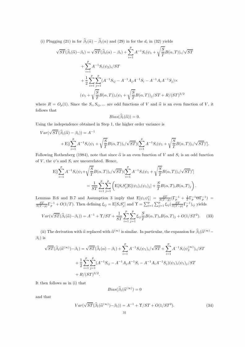
(i) Plugging (21) in for β1(α) − β1(α) and (29) in for the di in (32) yields

√ST (β1(α)−β1) =

√ST (β1(α) − β1) +

p∑

i=1

A−1Si(ψ1 +

√S

TB(α, T ))i/

√ST

+

p∑

i=1

A−1Si(ψ2)i/ST

+1

2

p∑

i=1

p∑

j=1

(A−1Sij −A−1AjA−1Si −A−1AiA

−1Sj)×

(ψ1 +

√S

TB(α, T ))i(ψ1 +

√S

TB(α, T ))j/ST +R/(ST )3/2

where R = Op(1). Since the Si, Sij , ... are odd functions of V and α is an even function of V , it

follows that

Bias(β1(α)) = 0.

Using the independence obtained in Step 1, the higher order variance is

V ar(√ST (β1(α) − β1)) = A−1

+ E[(

p∑

i=1

A−1Si(ψ1 +

√S

TB(α, T ))i/

√ST )(

p∑

i=1

A−1Si(ψ1 +

√S

TB(α, T ))i/

√ST )′].

Following Rothenberg (1984), note that since α is an even function of V and Si is an odd function

of V , the ψ’s and Si are uncorrelated. Hence,

E[(

p∑

i=1

A−1Si(ψ1+

√S

TB(α, T ))i/

√ST )(

p∑

i=1

A−1Si(ψ1 +

√S

TB(α, T ))i/

√ST )′]

=1

ST

p∑

i=1

p∑

j=1

(E[SiS

′j ]E[(ψ1)i(ψ1)j ] +

S

TB(α, T )iB(α, T )j

).

Lemmas B.6 and B.7 and Assumption 3 imply that E[ψ1ψ′1] = ST

S(T−p) (Γ−1p + 1

T Γ−1p ΘΓ−1

p ) =ST

S(T−p)Γ−1p + O(1/T ). Then defining ξij = E[SiS

′j] and Υ =

∑pi=1

∑pj=1 ξij(

STS(T−p)Γ

−1p )ij yields

V ar(√ST (β1(α)−β1)) = A−1 + Υ/ST +

1

ST

p∑

i=1

p∑

j=1

ξijS

TB(α, T )iB(α, T )j +O(1/ST 2). (33)

(ii) The derivation with α replaced with α(∞) is similar. In particular, the expansion for β1(α(∞)−

β1) is

√ST (β1(α

(∞))−β1) =√ST (β1(α) − β1) +

p∑

i=1

A−1Si(ψ1)i/√ST +

p∑

i=1

A−1Si(ψ(∞)2 )i/ST

+1

2

p∑

i=1

p∑

j=1

(A−1Sij −A−1AjA−1Si −A−1AiA

−1Sj)(ψ1)i(ψ1)j/ST

+R/(ST )3/2.

It then follows as in (i) that

Bias(β1(α(∞)) = 0

and that

V ar(√ST (β1(α

(∞))−β1)) = A−1 + Υ/ST +O(1/ST 2). (34)

31

Finally, the O(1/ST 2) term in (33) and (34) is the same, so

V ar(√ST (β1(α) − β1)) − V ar(

√ST (β1(α

(∞)) − β1)) =1

ST

p∑

i=1

p∑

j=1

ξijS

TB(α, T )iB(α, T )j

is positive semidefinite since

1

ST

p∑

i=1

p∑

j=1

ξijS

TB(α, T )iB(α, T )j =

1

ST

S

TE[(

p∑

i=1

B(α, T )iSi)(

p∑

j=1

B(α, T )jS′j)].

References

Alvarez, J., and M. Arellano (2003): “The Time Series and Cross-Section Asymptotics of DynamicPanel Data Estimators,” Econometrica, 71(4), 1121–1159.

Amemiya, T. (1978): “A Note on a Random Coefficient Model,” International Economic Review, 19(3),793–796.

Arellano, M. (1987): “Computing Robust Standard Errors for Within-Groups Estimators,” Oxford Bul-letin of Economics and Statistics, 49(4), 431–434.

Bell, R. M., and D. F. McCaffrey (2002): “Computing Robust Standard Errors for Within-GroupsEstimators,” Mimeo RAND.

Bertrand, M., E. Duflo, and S. Mullainathan (2004): “How Much Should We Trust Differences-in-Differences Estimates?,” Quarterly Journal of Economics, 119(1), 249–275.

Bhargava, A., L. Franzini, and W. Narendranathan (1982): “Serial Correlation and the Fixed EffectsModel,” Review of Economic Studies, 49, 533–549.

Billingsley, P. (1995): Probability and Measure. New York: Wiley, third edn.Dickens, W. T. (1990): “Error Components in Grouped Data: Is It Ever Worth Weighting?,” Review ofEconomics and Statistics, 72(2), 328–333.

Donald, S., and K. Lang (2001): “Inference with Difference in Differences and Other Panel Data,”Mimeo.

Doukhan, P. (1994): Mixing: Properties and Examples, vol. 85 of Lecture Notes in Statistics (Springer-Verlag). New York: Springer-Verlag.

Fitzpatrick, P. M. (1996): Advanced Calculus: A Course in Mathematical Analysis. PWS PublishingCompany: Boston, Massachussetts.

Hahn, J., and G. M. Kuersteiner (2002): “Asymptotically Unbiased Inference for a Dynamic PanelModel with Fixed Effects When Both N and T Are Large,” Econometrica, 70(4), 1639–1657.

Hahn, J., and W. Newey (2002): “Jackknife and Analytical Bias Reduction for Nonlinear Panel Models,”Mimeo.

Hansen, C. B. (2004): Inference in Linear Panel Data Models with Serial Correlation and an Essay on theImpact of 401(k) Participation on the Wealth Distribution. Ph.D. Dissertation, Massachusetts Institute ofTechnology.

Hausman, J., and G. Kuersteiner (2003): “Differences in Differences Meets Generalized Least Squares:Higher Order Properties of Hypothesis Tests,” Mimeo.

Kezdi, G. (2002): “Robust Standard Errors Estimation in Fixed-Effects Panel Models,” Mimeo.Kiefer, N. M. (1980): “Estimation of Fixed-Effects Models for Time Series of Cross-Sections with ArbitraryIntertemporal Covariance,” Journal of Econometrics, 14, 195–202.

Kiviet, J. F. (1995): “On Bias, Inconsistency, and Efficiency of Various Estimators in Dynamic Panel DataModels,” Journal of Econometrics, 68, 53–78.

Lancaster, T. (2002): “Orthogonal Parameters and Panel Data,” Review of Economic Studies, 69, 647–666.

Lehmann, E. L. (1983): Theory of Point Estimation. New York: Wiley.Liang, K.-Y., and S. Zeger (1986): “Longitudinal Data Analysis Using Generalized Linear Models,”Biometrika, 73(1), 13–22.

Macurdy, T. E. (1982): “The Use of Time Series Processes to Model the Error Structure of Earnings in aLongitudinal Data Analysis,” Journal of Econometrics, 18(1), 83–114.

Moulton, B. R. (1986): “Random Group Effects and the Precision of Regression Estimates,” Journal ofEconometrics, 32(3), 385–397.

Newey, W. K., and R. J. Smith (2001): “Higher Order Properties of GMM and Generalized EmpiricalLikelihood Estimators,” Mimeo.

Nickell, S. (1981): “Biases in Dynamic Models with Fixed Effects,” Econometrica, 49(6), 1417–1426.Pfanzagl, J., and W. Wefelmeyer (1978): “A Third-Order Optimum Property of the Maximum Like-lihood Estimator,” Journal of Multivariate Analysis, 8, 1–29.

Phillips, P. C. B., and H. R. Moon (1999): “Linear Regression Limit Theory for Nonstationary PanelData,” Econometrica, 67(5), 1057–1111.

Rothenberg, T. J. (1984): “Approximate Normality of Generalized Least Squares Estimates,” Economet-rica, 52(4), 811–825.

32

Solon, G. (1984): “Estimating Autocorrelations in Fixed Effects Models,” NBER Technical Working PaperNo. 32.

White, H. (2001): Asymptotic Theory for Econometricians. San Diego: Academic Press, revised edn.Wooldridge, J. M. (2003): “Cluster-Sample Methods in Applied Econometrics,” American EconomicReview, 93(2), 133–188.

33

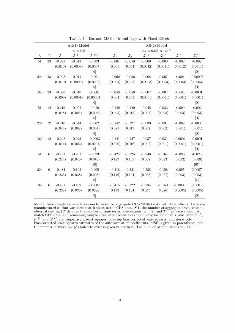
Table 1. Bias and MSE of α and αBC with Fixed Effects

AR(1) Model AR(2) Model

α1 = 0.8 α1 = 0.80, α2 = 0

S T bα bα(1) bα(∞) bα1 bα2 bα(1)1 bα(1)

2 bα(∞)1 bα(∞)

2

51 23 -0.099 -0.013 -0.003 -0.061 -0.058 -0.009 -0.008 -0.002 -0.002

(0.010) (0.0008) (0.0007) (0.005) (0.004) (0.0012) (0.0011) (0.0012) (0.0011)

[0] [0]

204 23 -0.098 -0.011 -0.001 -0.060 -0.056 -0.008 -0.007 -0.001 -0.00003

(0.010) (0.0003) (0.0002) (0.004) (0.003) (0.0003) (0.0003) (0.0003) (0.0003)

[0] [0]

1020 23 -0.096 -0.010 -0.0001 -0.059 -0.056 -0.007 -0.007 0.0001 -0.0001

(0.009) (0.0001) (0.00003) (0.004) (0.003) (0.0001) (0.0001) (0.0001) (0.0001)

[0] [0]

51 12 -0.216 -0.052 -0.010 -0.149 -0.129 -0.045 -0.033 -0.009 -0.002

(0.048) (0.005) (0.003) (0.025) (0.018) (0.005) (0.003) (0.003) (0.003)

[0] [0]

204 12 -0.210 -0.044 -0.002 -0.142 -0.127 -0.039 -0.031 -0.002 -0.0003

(0.044) (0.002) (0.001) (0.021) (0.017) (0.002) (0.002) (0.001) (0.001)

[0] [0]

1020 12 -0.208 -0.043 -0.0003 -0.141 -0.127 -0.037 -0.031 -0.0002 -0.0001

(0.044) (0.002) (0.0001) (0.020) (0.016) (0.002) (0.001) (0.0001) (0.0001)

[0] [0]

51 6 -0.491 -0.201 -0.023 -0.424 -0.325 -0.246 -0.164 -0.036 -0.020

(0.244) (0.046) (0.010) (0.187) (0.109) (0.068) (0.033) (0.012) (0.009)

[30] [67]

204 6 -0.484 -0.192 -0.005 -0.418 -0.321 -0.238 -0.158 -0.005 0.0007

(0.235) (0.038) (0.003) (0.176) (0.104) (0.058) (0.027) (0.003) (0.003)

[0] [4]

1020 6 -0.481 -0.189 -0.0007 -0.415 -0.322 -0.234 -0.159 -0.0006 0.0001

(0.232) (0.036) (0.0006) (0.172) (0.104) (0.055) (0.026) (0.0005) (0.0005)

[0] [0]

Monte Carlo results for simulation model based on aggregate CPS-MORG data with fixed effects. Data aremanufactured so that variances match those in the CPS data. S is the number of aggregate cross-sectionalobservations, and T denotes the number of time series observations. S = 51 and T = 23 were chosen tomatch CPS data, and remaining sample sizes were chosen to explore behavior for small T and large S. bα,bα(1), and bα(∞) are, respectively, least squares, one-step bias-corrected least squares, and iterativelybias-corrected least squares estimates of the autocorrelation coefficients. MSE is given in parentheses, andthe number of times α−1

T (bα) failed to exist is given in brackets. The number of simulations is 1000.

34

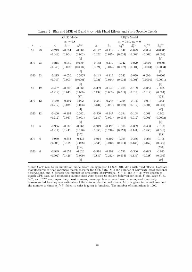
Table 2. Bias and MSE of α and αBC with Fixed Effects and State-Specific Trends

AR(1) Model AR(2) Model

α1 = 0.8 α1 = 0.80, α2 = 0

S T bα bα(1) bα(∞) bα1 bα2 bα(1)1 bα(1)

2 bα(∞)1 bα(∞)

2

51 23 -0.219 -0.054 -0.005 -0.147 -0.119 -0.047 -0.029 -0.004 -0.0005

(0.049) (0.004) (0.002) (0.023) (0.015) (0.004) (0.002) (0.002) (0.001)

[0] [3]

204 23 -0.215 -0.050 0.0003 -0.142 -0.119 -0.042 -0.029 0.0006 -0.0004

(0.046) (0.003) (0.0004) (0.021) (0.014) (0.002) (0.001) (0.0004) (0.0003)

[0] [0]

1020 23 -0.215 -0.050 -0.0005 -0.143 -0.119 -0.043 -0.029 -0.0004 -0.0002

(0.046) (0.003) (0.0001) (0.021) (0.014) (0.002) (0.001) (0.0001) (0.0001)

[0] [0]

51 12 -0.467 -0.200 -0.030 -0.369 -0.248 -0.203 -0.109 -0.054 -0.025

(0.219) (0.043) (0.009) (0.139) (0.063) (0.045) (0.014) (0.012) (0.004)

[87] [173]

204 12 -0.460 -0.192 0.002 -0.361 -0.247 -0.195 -0.108 -0.007 -0.006

(0.212) (0.038) (0.003) (0.131) (0.061) (0.039) (0.012) (0.004) (0.001)

[4] [45]

1020 12 -0.460 -0.192 -0.0001 -0.360 -0.247 -0.194 -0.108 0.001 -0.001

(0.212) (0.037) (0.001) (0.130) (0.061) (0.038) (0.012) (0.001) (0.0002)

[0] [0]

51 6 -0.955 -0.660 -0.262 -0.919 -0.493 -0.803 -0.369 -0.403 -0.162

(0.914) (0.441) (0.126) (0.850) (0.246) (0.653) (0.141) (0.253) (0.046)

[270] [318]

204 6 -0.950 -0.653 -0.135 -0.914 -0.492 -0.795 -0.366 -0.268 -0.106

(0.903) (0.428) (0.068) (0.836) (0.242) (0.634) (0.135) (0.162) (0.029)

[152] [230]

1020 6 -0.949 -0.652 -0.020 -0.914 -0.492 -0.796 -0.366 -0.083 -0.023

(0.902) (0.426) (0.009) (0.835) (0.242) (0.634) (0.134) (0.028) (0.005)

[8] [28]

Monte Carlo results for simulation model based on aggregate CPS-MORG data with fixed effects. Data aremanufactured so that variances match those in the CPS data. S is the number of aggregate cross-sectionalobservations, and T denotes the number of time series observations. S = 51 and T = 23 were chosen tomatch CPS data, and remaining sample sizes were chosen to explore behavior for small T and large S. bα,bα(1), and bα(∞) are, respectively, least squares, one-step bias-corrected least squares, and iterativelybias-corrected least squares estimates of the autocorrelation coefficients. MSE is given in parentheses, andthe number of times α−1

T (bα) failed to exist is given in brackets. The number of simulations is 1000.

35

Table 3. Estimated Variance of Treatment Parameter in Simulated AR(1) Model with α = .8.

S = 51, T = 23 S = 51, T = 12 S = 51, T = 6bσ2 σ2a σ2

s bσ2 σ2a σ2

s bσ2 σ2a σ2

s

A. Conventional Inference Methods

OLS 0.024 0.108 0.107 0.035 0.101 0.109 0.046 0.078 0.081

OLS - Cluster by state 0.102 0.108 0.107 0.096 0.101 0.109 0.075 0.078 0.081

FGLS-U 0.020 0.037 0.062 0.030 0.040 0.049 0.038 0.044 0.051

AR(1) 0.034 0.037 0.039 0.038 0.040 0.046 0.045 0.044 0.060

AR(1) - Cluster by state 0.037 0.037 0.039 0.044 0.040 0.046 0.054 0.044 0.060

AR(2) 0.034 0.037 0.040 0.038 0.040 0.046 0.045 0.044 0.060

AR(2) - Cluster by state 0.038 0.037 0.040 0.045 0.040 0.046 0.055 0.044 0.060

B. FGLS with Bias-Corrected AR Coefficients

AR(1)bc 0.037 0.037 0.037 0.040 0.040 0.038 0.044 0.044 0.046

AR(1)bc - Cluster by state 0.035 0.037 0.037 0.039 0.040 0.038 0.041 0.044 0.046

AR(2)bc 0.037 0.037 0.037 0.040 0.040 0.038 0.044 0.044 0.046

AR(2)bc - Cluster by state 0.035 0.037 0.037 0.038 0.040 0.038 0.041 0.044 0.046

Monte Carlo results for simulation model based on aggregate CPS-MORG data. Data are manufactured sothat variances correspond to those in the CPS data, and the error process is assumed to follow an AR(1)with α = .8. S is the number of aggregate cross-sectional observations, and T denotes the number of timeseries observations. S = 51 and T = 23 correspond to the full sample of CPS data, and remaining samplesizes were chosen to explore behavior for small T . Results are for the variance of the treatment parameter,β1, only. bσ2 is 1000 times the mean of the estimated variances, σ2

a is 1000 times the asymptotic variance,and σ2

s is 1000 times the variance of the β1’s estimated in the simulation. The number of simulations is1000.

36

Table 4. Monte Carlo Results from CPS-MORG Microdata

S = 51, T = 23 S = 51, T = 12 S = 51, T = 6

Size Power Length Size Power Length Size Power Length

A. Conventional Inference Methods

OLS 0.594 0.860 0.006 0.398 0.866 0.009 0.072 0.850 0.012

(0.022) (0.016) (0.022) (0.015) (0.012) (0.016)

OLS - Cluster 0.078 0.354 0.024 0.078 0.548 0.019 0.064 0.798 0.013

by state (0.012) (0.021) (0.012) (0.022) (0.011) (0.018)

Random Effects - 0.392 0.778 0.010 0.222 0.870 0.011 0.050 0.808 0.013

state × year (0.022) (0.019) (0.019) (0.015) (0.009) (0.018)

OLS - Cluster by 0.398 0.766 0.011 0.280 0.804 0.011 0.076 0.844 0.012

state × year (0.022) (0.019) (0.020) (0.018) (0.012) (0.016)

B. FGLS with Bias-Corrected AR Coefficients

AR(2)bc 0.078 0.714 0.015 0.152 0.880 0.012 0.050 0.804 0.014

(0.012) (0.020) (0.016) (0.015) (0.010) (0.018)

AR(2)bc - Cluster 0.078 0.728 0.016 0.070 0.880 0.015 0.058 0.792 0.014

by state (0.012) (0.020) (0.011) (0.015) (0.010) (0.018)

AR(3)bc 0.076 0.738 0.015 0.142 0.888 0.012

(0.012) (0.020) (0.016) (0.014)

AR(3)bc - Cluster 0.076 0.744 0.015 0.072 0.774 0.015

by state (0.012) (0.020) (0.012) (0.019)

Monte Carlo results for simulation model using individual CPS-MORG data. Data are manufactured byresampling states from actual CPS-MORG data. S is the number of aggregate cross-sectional observations,and T denotes the number of time series observations. S = 51 and T = 23 correspond to the full sample ofCPS data, and remaining sample sizes were chosen to explore behavior for small T . Results are for thetreatment parameter which enters the model with a true coefficient of β1 = 0. Size and power are for 5%level tests, and power is versus the alternative that β1 = .02. Length is the 95% confidence interval lengthdivided by two. Interval lengths are based on a t50 for tests with standard errors clustered at the statelevel, a tST−1 for tests with standard errors clustered at the state × year level, and a N(0, 1) for theremaining tests. Simulation standard errors are reported in parentheses. (For interval length, thesimulation standard error is negligible, so it is not reported.) The number of simulations is 500.

37

Table 5. Monte Carlo Results from Aggregate CPS-MORG Data

S = 51, T = 23 S = 51, T = 12 S = 51, T = 6

Size Power Length Size Power Length Size Power Length

A. Conventional Inference Methods

OLS 0.374 0.762 0.011 0.158 0.846 0.012 0.052 0.730 0.015

(0.022) (0.019) (0.016) (0.016) (0.010) (0.020)

OLS - Cluster 0.066 0.344 0.025 0.062 0.656 0.017 0.052 0.744 0.015

by state (0.011) (0.021) (0.011) (0.021) (0.010) (0.020)

FGLS-U 0.362 0.962 0.007 0.112 0.932 0.010 0.086 0.804 0.013

(0.021) (0.009) (0.014) (0.011) (0.013) (0.018)

AR(2) 0.104 0.772 0.014 0.116 0.844 0.014 0.080 0.774 0.014

(0.014) (0.019) (0.014) (0.016) (0.012) (0.019)

AR(2) - Cluster 0.064 0.662 0.016 0.062 0.726 0.016 0.048 0.716 0.015

by state (0.011) (0.021) (0.011) (0.020) (0.010) (0.020)

AR(3) 0.106 0.770 0.014 0.132 0.834 0.013

(0.014) (0.019) (0.015) (0.017)

AR(3) - Cluster 0.072 0.688 0.016 0.068 0.708 0.016

by state (0.012) (0.021) (0.011) (0.020)

B. FGLS with Bias-Corrected AR Coefficients

AR(2)bc 0.080 0.750 0.015 0.064 0.814 0.014 0.042 0.720 0.015

(0.012) (0.019) (0.011) (0.017) (0.009) (0.020)

AR(2)bc - Cluster 0.062 0.754 0.015 0.062 0.800 0.014 0.060 0.734 0.015

by state (0.011) (0.019) (0.011) (0.018) (0.011) (0.020)

AR(3)bc 0.064 0.766 0.014 0.066 0.810 0.014

(0.011) (0.019) (0.011) (0.018)

AR(3)bc - Cluster 0.076 0.788 0.014 0.060 0.808 0.014

by state (0.012) (0.018) (0.011) (0.018)

Monte Carlo results for simulation model using aggregate CPS-MORG data. Data are manufactured byresampling states from actual CPS-MORG data and aggregating data to the state-year level using themethod of Amemiya (1978) outlined in the text. S is the number of aggregate cross-sectional observations,and T denotes the number of time series observations. S = 51 and T = 23 correspond to the full sample ofCPS data, and remaining sample sizes were chosen to explore behavior for small T . Results are for thetreatment parameter which enters the model with a true coefficient of β1 = 0. Size and power are for 5%level tests, and power is versus the alternative that β1 = .02. Length is the 95% confidence interval lengthdivided by two. Interval lengths are based on a t50 for tests with standard errors clustered at the statelevel and a tST−S−T for the remaining tests. Simulation standard errors are reported in parentheses. (Forinterval length, the simulation standard error is negligible, so it is not reported.) The number ofsimulations is 500.

38

Table 6. Monte Carlo Results from Simulated AR(1) Model with α = .8.

S = 51, T = 23 S = 51, T = 12 S = 51, T = 6

Size Power Length Size Power Length Size Power Length

A. Conventional Inference Methods

OLS 0.356 0.842 0.010 0.285 0.794 0.012 0.141 0.730 0.013

(0.015) (0.011) (0.014) (0.013) (0.011) (0.014)

OLS - Cluster 0.056 0.490 0.020 0.065 0.520 0.020 0.058 0.574 0.017

by state (0.007) (0.016) (0.008) (0.016) (0.007) (0.016)

FGLS-U 0.269 0.915 0.009 0.121 0.900 0.011 0.091 0.834 0.012

(0.014) (0.008) (0.011) (0.009) (0.009) (0.012)

AR(1) 0.078 0.914 0.011 0.077 0.878 0.012 0.083 0.786 0.013

(0.008) (0.009) (0.008) (0.011) (0.008) (0.013)

AR(1) - Cluster 0.057 0.884 0.012 0.059 0.830 0.013 0.064 0.728 0.015

by state (0.007) (0.010) (0.008) (0.012) (0.008) (0.014)

AR(2) 0.080 0.912 0.011 0.081 0.874 0.012 0.093 0.778 0.013

(0.008) (0.009) (0.008) (0.011) (0.009) (0.013)

AR(2) - Cluster 0.062 0.882 0.012 0.060 0.828 0.013 0.064 0.724 0.015

by state (0.008) (0.010) (0.008) (0.012) (0.008) (0.014)

B. FGLS with Bias-Corrected AR Coefficients

AR(1)bc 0.056 0.908 0.012 0.044 0.880 0.012 0.062 0.818 0.013

(0.007) (0.009) (0.006) (0.011) (0.008) (0.012)

AR(1)bc - Cluster 0.061 0.904 0.012 0.050 0.874 0.012 0.069 0.822 0.013

by state (0.008) (0.009) (0.007) (0.011) (0.008) (0.012)

AR(2)bc 0.057 0.904 0.012 0.044 0.882 0.012 0.066 0.822 0.013

(0.007) (0.009) (0.006) (0.010) (0.008) (0.012)

AR(2)bc - Cluster 0.065 0.900 0.012 0.049 0.880 0.012 0.070 0.824 0.013

by state (0.008) (0.009) (0.007) (0.011) (0.008) (0.012)

Monte Carlo results for simulation model based on aggregate CPS-MORG data. Data are manufactured sothat variances correspond to those in the CPS data, and the error process is assumed to follow an AR(1)with α = .8. S is the number of aggregate cross-sectional observations, and T denotes the number of timeseries observations. S = 51 and T = 23 correspond to the full sample of CPS data, and remaining samplesizes were chosen to explore behavior for small T . Results are for the treatment parameter which entersthe model with a true coefficient of β1 = 0. Size and power are for 5% level tests, and power is versus thealternative that β1 = .02. Length is the 95% confidence interval length divided by two. Interval lengths arebased on a t50 for tests with standard errors clustered at the state level and a tST−S−T for the remainingtests. Simulation standard errors are reported in parentheses. (For interval length, the simulation standarderror is negligible, so it is not reported.) The number of simulations is 1000.

39

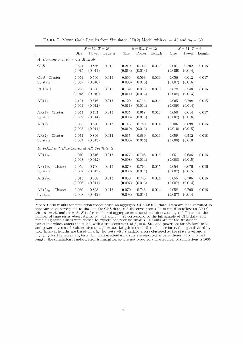
Table 7. Monte Carlo Results from Simulated AR(2) Model with α1 = .43 and α2 = .30.

S = 51, T = 23 S = 51, T = 12 S = 51, T = 6

Size Power Length Size Power Length Size Power Length

A. Conventional Inference Methods

OLS 0.324 0.856 0.010 0.210 0.764 0.012 0.091 0.702 0.015

(0.015) (0.011) (0.013) (0.013) (0.009) (0.014)

OLS - Cluster 0.054 0.536 0.019 0.063 0.508 0.019 0.058 0.612 0.017

by state (0.007) (0.016) (0.008) (0.016) (0.007) (0.016)

FGLS-U 0.233 0.890 0.010 0.132 0.813 0.013 0.078 0.746 0.015

(0.013) (0.010) (0.011) (0.012) (0.008) (0.013)

AR(1) 0.101 0.816 0.013 0.120 0.744 0.014 0.095 0.708 0.015

(0.009) (0.012) (0.011) (0.014) (0.009) (0.014)

AR(1) - Cluster 0.054 0.744 0.015 0.065 0.658 0.016 0.058 0.614 0.017

by state (0.007) (0.014) (0.008) (0.015) (0.007) (0.016)

AR(2) 0.065 0.850 0.013 0.115 0.750 0.014 0.106 0.698 0.015

(0.008) (0.011) (0.010) (0.013) (0.010) (0.015)

AR(2) - Cluster 0.051 0.806 0.014 0.065 0.680 0.016 0.059 0.582 0.018

by state (0.007) (0.013) (0.008) (0.015) (0.008) (0.016)

B. FGLS with Bias-Corrected AR Coefficients

AR(1)bc 0.070 0.816 0.013 0.077 0.708 0.015 0.061 0.686 0.016

(0.008) (0.012) (0.008) (0.014) (0.008) (0.015)

AR(1)bc - Cluster 0.059 0.766 0.015 0.070 0.704 0.015 0.054 0.676 0.016

by state (0.008) (0.013) (0.008) (0.014) (0.007) (0.015)

AR(2)bc 0.043 0.838 0.013 0.053 0.746 0.014 0.055 0.706 0.016

(0.006) (0.011) (0.007) (0.013) (0.007) (0.014)

AR(2)bc - Cluster 0.060 0.828 0.013 0.070 0.746 0.014 0.058 0.700 0.016

by state (0.008) (0.012) (0.008) (0.013) (0.007) (0.014)

Monte Carlo results for simulation model based on aggregate CPS-MORG data. Data are manufactured sothat variances correspond to those in the CPS data, and the error process is assumed to follow an AR(2)with α1 = .43 and α2 = .3. S is the number of aggregate cross-sectional observations, and T denotes thenumber of time series observations. S = 51 and T = 23 correspond to the full sample of CPS data, andremaining sample sizes were chosen to explore behavior for small T . Results are for the treatmentparameter which enters the model with a true coefficient of β1 = 0. Size and power are for 5% level tests,and power is versus the alternative that β1 = .02. Length is the 95% confidence interval length divided bytwo. Interval lengths are based on a t50 for tests with standard errors clustered at the state level and atST−S−T for the remaining tests. Simulation standard errors are reported in parentheses. (For intervallength, the simulation standard error is negligible, so it is not reported.) The number of simulations is 1000.

40