GENERALIZED LEAST SQUARES ESTIMATIONOF PANEL WITH COMMON SHOCKS 1

Paolo ZaffaroniImperial College LondonThis draft: 13 February 2009

Abstract

This paper considers GLS estimation of linear panel models whenthe innovation and the regressors can both contain a factor struc-ture. A novel feature of this approach is that preliminary estimationof the latent factor structure is not necessary. Under a set of regular-ity conditions here provided, we establish consistency and asymptoticnormality of the feasible GLS estimator as both the cross-section andtime series dimensions diverge to infinity. Dependence, both tempo-rally and cross-sectionally, of the idiosyncratic innovation is permit-ted. Our results are presented separately for time regressions withunit-specific coefficients as well as for cross-section regressions withtime-specific coefficients. As particular cases of our set up, we estab-lish primitive conditions of our assumptions for Andrews (2005) andPesaran (2006) regression models. A set of Monte Carlo experimentscorroborate our results.

1 Introduction

Factor models represent one of the most popular and successful way to cap-ture cross-sectional dependence, especially when facing a large number ofunits (N). However, a factor structure in the innovation of a linear regres-sion model can make the ordinary least squares (henceforth OLS) estimatorinvalid since it will no longer be consistent, in general, for the true regressioncoefficients unless some restrictions are imposed. In a linear cross-sectionalregression with constant parameters Andrews (2005) shows that consistencyof the OLS estimator is preserved, as N goes to infinity, when both the errorand the regressors have a factor structure with uncorrelated factor load-ings. The parameters estimate has a mixed normal asymptotic distribution.Within a linear regression across time (T ) with the innovation and the re-gressors sharing a factor structure, when a panel of observations is available,Pesaran (2006) shows that individual-specific regression coefficients can be

1

consistently estimated by augmenting the regressors by cross-sectional av-erages of the dependent and the individual-specific regressors. The conven-tional asymptotic normality is obtained, as both N, T go to infinity. Again,the essential condition is a restriction on the joint distribution of the factorsloadings for the factor structure in the regressors and innovation, namelythat their (population) means must be linearly independent.

This paper considers cross-sectional regressions with time-specific param-eters as well as time regressions with individual-specific parameters when theinnovation contains a factor structure and a panel of data is available. Bothcases are of independent interest. It is here noted that, in either cases, theunfeasible generalized least squares (henceforth UGLS) estimator, based onthe presumption that the covariance matrix of the factor structure is known,would be consistent and asymptotically normal distributed without any par-ticular restriction on the factor loadings nor on the common factors, in par-ticular even if the innovation and the regressors are mutually correlated. Thisis due to a form of asymptotic orthogonality between the factor loadings andthe inverse of the factor structure covariance matrix. The difficulty ariseswhen considering a feasible version of the GLS estimator. A natural approachwould be, exploiting the panel dimension, to consider the sample covariancematrix of the OLS residuals. Given the non-consistency of the OLS estima-tor, such sample covariance matrix would also be non-consistent for the truecovariance matrix. However, the relevant result here is that, under suitableregularity conditions, the limit of such sample covariance matrix leads to amatrix whose inverse is also asymptotically orthogonal to the factor loadings.Indeed, there is an entire class of matrices, rather than a unique matrix, thatis asymptotically orthogonal to the factor loadings. As a consequence, weshow that this feasible GLS (henceforth GLS) estimator is consistent andasymptotically normal, as both N, T diverge to infinity, under a set of con-ditions that make the OLS invalid. However, the limit covariance matrix ofthe OLS residuals will be in general different from the true covariance matrixof true innovations, and thus such the GLS might not be as efficient as theUGLS.

The GLS estimator exhibits a number of desirable properties. First, it iscomputationally easy to handle since it simply requires to perform a sequenceof linear regressions. Second, the GLS estimator does not require knowledgeof the number of factors nor of estimates of the factors themselves since it isnot based on a preliminary estimation of the factor structure. Thus, we donot need to make use of the recent advances in estimation of (dynamic) factor

2

models such as Forni, Hallin, Lippi, and L. (2000), Bai and Ng (2002), Stockand Watson (2002) and Bai (2003), which in turn would require preliminarytesting of the number of factors (Bai and Ng (2002) and Hallin and Liska(2007) for tests designed for static and dynamic factor models, respectively).

Panel with factor structure innovations have also been considered byHoltz-Eakin, Newey, and Rosen (1988), Ahn, Hoon Lee, and Schmidt (2001),Bai and Ng (2004) Phillips and Sul (2003), Moon and Perron (2003), andPhillips and Sul (2007). With the exception of Ahn, Hoon Lee, and Schmidt(2001), who focus on generalized method of moment estimation of cross-sectional regressions with independent and identically distributed (i.i.d.) re-gressors for fixed T the other papers are all defined within the context ofdynamic panel models. In particular, Holtz-Eakin, Newey, and Rosen (1988)note how the individual effects can be eliminated by quasi-differencing al-though this induces time-variation to otherwise constant regression coeffi-cients. They consider the asymptotic properties of an instrumental variableestimator for large N where the number of instruments is of order O(T 2). Forautoregressive panel models with possibly a time trend, Bai and Ng (2004)study unit root tests that permit to identify whether the non-stationarity isassociated with the factor structure part of with the idiosyncratic part. Theydo not treat the factor structure as a nuisance parameter but build their teston pre-estimated factors and idiosyncratic component by principal compo-nents, providing the asymptotic properties of the test for large N, T . For thesame models, Phillips and Sul (2003) focus on median unbiased estimation ofthe autoregressive parameter, and related homogeneity and unit root tests.Their asymptotic theory holds for fixed N . Moon and Perron (2003) proposeunit root testing with respect to a similar class of models, valid for bothlarge N, T , based on de-factoring the data by means of principal componentsestimation of the factor structure which if ignored, would substantially re-duce the power of the test. Their test has no power when linear trend withfixed effects is allowed for. For a larger class of dynamic panels, that allowsfor exogenous regressors, Phillips and Sul (2007) characterize the bias of the(pooled) OLS estimator for large N , in particular showing that it convergesto a random variable because of the substantial degree of cross-sectional de-pendence associated with the factor structure innovation.

Factor models is not the only way to describe cross-sectional dependence.Weaker, in the sense of local, forms of dependence can be achieved by spa-tial econometrics approaches, in particular spatial autoregressive models (seeAnselin (1988), Case (1991), Conley (1999), Chen and Conley (2001), Lee

3

(2004), Robinson (2006)).This paper, which studies separately the cases of estimation of linear

regressions with either individual-specific or time-specific parameters, pro-ceeds as follows. The next section illustrates the basic definitions and thegeneral assumptions required for estimation of regressions with unit-specificparameters stating with a theorem the asymptotic properties of the OLS,UGLS and GLS estimator as T , in the first two cases, and as N, T in thelast case, diverge to infinity. Section 2.3 then considers, as a special case, theregression model with unit-specific parameters of Pesaran (2006), establish-ing primitive conditions for our general assumptions. In particular, we showhow some, but not all, of these conditions are implied by certain of Pesaran’s(2006) assumptions, summarizing the findings in a proposition. Section 3 fo-cuses regression models with time-specific parameters, again presenting thebasic definitions and the general assumptions, summarizing the asymptoticproperties of the OLS, UGLS and GLS as N and N, T , respectively, divergeto infinity. Since Andrews (2005) cross-sectional model represents a specialcase of this set-up, section 3.3 investigates the extent to which Andrew’s(2005) assumptions provide primite conditions for at least some our generalassumptions. The full set of required primitive conditions is then describedin a proposition. The theoretical results are corroborated by a set of MonteCarlo experiments described in section 4. Section 5 concludes. The proofs ofboth theorems are reported in the final appendix.

Hereafter we use the following notation: →p denotes convergence in prob-ability and →d convergence in distribution. When A > 0 we mean thatthe matrix A is positive definite, A ≥ 0 that A is positive semi definite,‖ A ‖= (tr(AA′))

12 indicates the Euclidean norm of the matrix A, ιn is a

n×1 vector of ones, µi,a = Eai for a random vector ai and Σi,aCb′ is the limitin probability of A′

iCiBi/T for random matrices Ai,Bi with T rows and afinite number of columns and for the random T × T matrix Ci all possiblydependent on an index i. When Ci equals the identity matrix IT , we writeΣi,ab′ . We skip dependence on the index i when not necessary.

4

2 Unit-Specific Parameters Model

2.1 Definitions and assumptions

Throughout this section, the observed variables obey a linear regressionmodel with a k × 1 vector of possible unit-specific regression coefficientsβi0. The model for the ith unit can be expressed, in matrix form, as

yi = Xiβi0 + ui, (1)

for an observed T × 1 vector yi = (yi1, ..., yit, ..., yiT )′, an observed T × kmatrix Xi = (xi1, ...,xiT )′ where either none, some or even all of the re-gressors can be common across units, and an unobserved T × 1 vector ui =(ui1, ..., uit, ..., uiT )′. The innovation satisfy the factor structure

ui = Fbi + εi, (2)

for an unobserved m× 1 vector of factor loadings bi, an unobserved T ×mmatrix of common factors F = (f1, ..., fT )′ and an unobserved T × 1 vector ofidiosyncratic innovations εi = (εi1, ..., εiT )′. The maintained assumption hereis that k and m do not vary with T and N . Although model (1) is writtenas a regression across time, we assume that in fact a panel of observationsy,X = y1, ...,yi, ...,yN ,X1, ...,Xi, ...,XN is available. As pointed outin Pesaran (2006, section 2), several panel models, with either constant orunit-specific regression coefficients, are encompassed by his model, which inturn is a particular case of (1), including the traditional fixed and randomeffects models.

We now specify a set of general assumptions required for the estimatorshere considered, commenting on them through a series of remarks below.We then state, in Theorem 1, the asymptotic properties of the OLS, UGLSand GLS estimators for βi0. In the subsequent section we establish a setof primitive conditions of our general assumptions for the particular case ofinterest of model (1) given by Pesaran (2006) model.

Assumption 1.H (factor loadings)For every i, the bi are random vector of dimension m× 1 such that E(bib

′i |

Xi,F) = Bi > 0 with N−1∑N

i=1 Bi →p B > 0 as N →∞.

Assumption 2.H (idiosyncratic innovation)

5

For every i, εi = (εi1, ..., εit, ..., εiT )′ satisfies E(εi | bi, Xi,F) = 0 and

Hi = E(εiε′i | bi, Xi,F) > 0, (3)

N−1

N∑i=1

Hi →p HT > 0 as N →∞. (4)

Assumption 3.H (regressors)For every i, the T × k matrix Xi is full column rank.

Assumption 4.H (basic limit conditions)All the limit matrices below, as T →∞, are a.s. finite:

X′iXi

T→p Σi,xx′ > 0,

X′iHiXi

T→p Σi,xHx′ > 0,

X′iF

T→p Σi,xf ′ , (5)

X′iH

−1i Xi

T→p Σi,xH−1x′ > 0,

F′H−1i F

T→p Σi,fH−1f ′ > 0,

X′iH

−1i F

T→p Σi,xH−1f ′ ,

(6)

such thatΣi,xH−1x′ −Σi,xH−1f ′Σi,fH−1f ′Σ

′i,xH−1f ′ > 0. (7)

Assumption 5.H (limit conditions for GLS)All the limit matrices below, as N →∞ and arbitrary T , are a.s. finite:

N∑i=1

XiΣ−1i,xx′Σi,xf ′bib

′iΣ

′i,xf ′Σ

−1i,xx′X

′i

N= A1T (1+op(1)),

N∑i=1

XiΣ−1i,xx′Σi,xf ′bib

′iF′

N= A2T (1+op(1)),

N∑i=1

XiΣ−1i,xx′X

′iεiε

′iXiΣ

−1i,xx′X

′i

NT= A3T (1 + op(1)),

N∑i=1

XiΣ−1i,xx′X

′iεiε

′i

N= A4T (1 + op(1)),

N∑i=1

biε′i

N12

= C1T (1 + op(1)),N∑

i=1

XiΣ−1i,xx′Σi,xf ′biε

′i

N12

= C2T (1 + op(1)), (8)

N∑i=1

biε′iXiΣ

−1i,xx′X

′i

N12 T

12

= C3T (1 + op(1)),N∑

i=1

XiΣ−1i,xx′Σi,xf ′biε

′iXiΣ

−1i,xx′X

′i

N12 T

12

= C4T (1 + op(1)). (9)

Assumption 6.H (distribution conditions for OLS and UGLS)

6

As T →∞:

X′iεi

T12

→d N (0,Σi,xHx′), (10)

X′iH

−1i εi

T12

→d N (0,Σi,xH−1x′),F′H−1

i εi

T12

→d N (0,Σi,fH−1f ′). (11)

Assumption 7.H (distribution and identification conditions for GLS)Let D1T , E1T be m×m matrices and D2T , E2T be T × T matrices satisfying

A1T − (A2T +A′2T ) = FD1TF′ +D2T and A3T − (A4T +A′

4T ) = FE1TF′ + E2T (12)

with an m×m non-singular symmetric I1T = D1T +T−1E1T +B and a T ×Tnon-singular I2T = D2T + T−1E2T +HT satisfying a.s.:

F′I−12T F

T→p ΣfI−1

2 f ′ (non-singular),F′I−1

2T HiI−12T F

T→p Σi,fI−1HI−1

2 f ′ ,(13)

X′iI−1

2T Xi

T→p Σi,xI−1

2 x′ (non-singular),X′

iI−12T HiI−1

2T Xi

T→p Σi,xI−1

2 HI−12 x′ ,

X′iI−1

2T F

T→p Σi,xI−1

2 f ′ ,X′

iI−12T HiI−1

2T F

T→p Σi,xI−1

2 HI−12 f ′ ,

X′iI−1

2T εi

T12

→d N (0,Σi,xI−12 HI−1

2 x′),F′I−1

2T εi

T12

→d N (0,Σi,fI−12 HI−1

2 f ′),

where all the limits above hold as T →∞ with a.s. finite limit matrices and,setting

ΣT = FI1TF′ + I2T ,

for all i and some a, b, c, d > 0:

X′iΣ

−1T (FC1T + C ′1TF′ + C2T + C ′2T )Σ−1

T (Fbi + εi) = Op(Taιk), (14)

X′iΣ

−1T (FC3T + C ′3TF′ + C4T + C ′4T )Σ−1

T (Fbi + εi) = Op(Tbιk), (15)

X′iΣ

−1T (FC1T + C ′1TF′ + C2T + C ′2T )Σ−1

T Xi = Op(Tcιkι

′k), (16)

X′iΣ

−1T (FC3T + C ′3TF′ + C4T + C ′4T )Σ−1

T Xi = Op(Tdιkι

′k). (17)

Remarks: 1. We are assuming that the factor loadings bi are unobservedrandom variables with a non-singular yet possibly heterogeneous distribution,varying with the index i. We do not necessarily require the bi to be mutu-ally independent from the regressors and from the factors although mutualindependence is typically assumed for concrete models.

7

2. The factors ft are assumed unobserved, whereas observed factors, if present,will be simply part of the regressors Xi. Moreover, there is no restriction onthe time dependence of the ft, who can be autocorrelated. One of the suffi-cient conditions for Assumption 7.H will be, however, bounded-ness of Σff ′ .Hence the ft can satisfy for instance a stationary vector auto-regression.3. The idiosyncratic innovation εi does not need to be i.i.d across i, nor needsto be independent from either the factor loadings bi, the factors F and theobserved regressors Xi. Moreover, Hi can vary with i and does not need tobe diagonal, implying a substantial degree of both heterogeneity as well asthe possibility of time dependence time dependence.4. Assuming full column rank of Xi for all i is required, given that computa-tionally the GLS estimator relies on the evaluation of a sequence of N OLSproblems.5. When Σi,xx′ and Σff ′ are finite, then the other limit matrices are finite bySchwartz inequality requiring, for certain cases, that the maximum eigenvalueof Hi is bounded and its minimum eigenvalue is bounded away from zero,uniformly in T . Bounded-ness of the maximum eigenvalue is implied whenui satisfy an approximate factor structure Chamberlain (1983).

Note that Σi,xf ′ represents the cross-correlation (when EF = 0) betweenthe regressors Xi and the factors F and it determines the non-zero asymptoticbias of the OLS estimator, unless it is a matrix of zeros or, if not, for thetrivial case of no factor structure (bi = 0). Under our assumptions, theregression innovation ui has covariance matrix

Si = FBiF′ + Hi

and, as seen below, the UGLS estimator of βi0 requires the limit of T−1X′iS−1i Xi

to be positive definite, as stated in (7).6. The limit matrices in Assumptions 5.H and 7.H arise when looking at theprobability limit of the sample covariance matrix of the OLS innovations.Similarly, the limiting distribution results stated in Assumptions 6.H and7.H, are required for OLS, UGLS and GLS respectively. Since we aim atproviding general results, we do not specify here the primitive conditionsrequired, although these can be relatively easily established when one con-siders particular cases of (1) such as for Pesaran (2006)’s model, examinedin section 2.3.7. As explained below, considering the GLS will imply to consider ΣT inplace of Si. Therefore, the various conditions dictated by Assumption 7.H

8

on I1T , I2T make sure that Σ−1T will be (as S−1

i ) asymptotically orthogonal tothe matrix of latent factors F. This is the essential property that guaranteesthat the GLS estimator will have good asymptotic properties.8. Conditions (14)-(17) determine the speed at which N and T have to divergeto infinity, possibly at different rates, to ensure that the GLS estimator isconsistent and asymptotically normal.

2.2 Estimators results

For estimation of parameters βi0, the OLS estimator yield

βOLSi = (X′

iXi)−1Xiyi,

The unfeasible generalized least squares (UGLS) estimator is

βUGLSi = (X′

iS−1i Xi)

−1XiS−1i yi,

settingSi = FBiF

′ + Hi.

The feasible generalized least squares (GLS) estimator is

βGLSi = (X′

iΣ−1T Xi)

−1XiΣ−1T yi,

setting

ΣT = N−1

N∑i=1

uiu′i, ui = yi −Xiβ

OLSi .

This requires at minimum N ≥ T . Note, however, that if the regressorscontain some observed factors, such as for instance when an intercept term isallowed for, which can be written, without loss of generality, as Xi = (D,X∗

i )for a T × k1 matrix D and a T × k2 matrix X∗

i , where k = k1 + k2, thenu′1D = 0 for all i. As a consequence, ΣT will be at most of rank T − k1 < T ,no matter how large N is. Therefore, to allow non-singularity we considerinstead the alternative definition

ΣT = N−1

N∑i=1

uiu′i + T−1DD′,

where the normalization by T−1 is required since, from our assumptions,supT ‖Σ−1

T ‖= O(1) a.s.

9

Theorem 1 (unit-specific parameters)

(i) (OLS) When Assumptions 3.H, 4.H.(5), 6.H.(10) hold

T12 (βOLS

i − βi0 − γOLSi ) →d Nk(0,VOLS

i ) as T →∞,

settingγOLS

i = Σ−1i,xx′Σi,xf ′bi, VOLS

i = Σ−1i,xx′Σi,xHx′Σ

−1i,xx′ .

(ii) (UGLS) When Assumptions 1.H, 2.H.(3), 3.H, 4.H.(6), 6.H.(11)

T12 (βUGLS

i − βi0) →d Nk(0,VUGLSi ) as T →∞,

settingVUGLS

i = (MUGLSi )−1N UGLS

i (MUGLSi )−1

withMUGLSi = plimT→∞ T−1(X′

iS−1i Xi), N UGLS

i = plimT→∞ T−1X′iS−1

i HiS−1i Xi.

Moreover(MUGLS

i )−1 = N UGLSi .

(iii) (GLS) When Assumptions 1.H, 2.H.(4), 3.H, 4.H.(5) and (7), 5.H,7.H

βGLSi →p βi0 as

1

T+

Tmax(a−1,b− 32)

N12

+Tmax(c− 3

2,d−2)

N12

→ 0,

T12 (βGLS

i − βi0) →d Nk(0,VGLSi ) as

1

T+

Tmax(a− 12,b−1)

N12

+Tmax(c−1,d− 3

2)

N12

→ 0,

settingVGLS

i = (MGLSi )−1NGLS

i (MGLSi )−1

withMGLSi = plim(N,T )→∞ T−1(X′

iΣ−1T Xi), NGLS

i = plim(N,T )→∞ T−1X′iΣ

−1T HiΣ

−1T Xi.

Remarks 1. The asymptotic bias of the OLS estimator is not simply ex-pressed in terms an un-centered asymptotic distribution which would other-wise still ensures consistency. Instead βOLS

i = βi0 + γOLSi + Op(T

− 12 ) where

γOLSi = Σ−1

i,xx′Σi,xf ′bi is a random variable. Consistency is achieved if ei-ther bi = 0, meaning no factor structure, or Σi,xf ′ = 0, that is zero cross-correlation between the regressors and the factors (assuming the latter havemean zero).

10

2. It is well-known that the UGLS estimator improves efficiency with respectthe the OLS estimator for non-spherical innovations. Here we find that UGLSexhibits a more profound property: it completely eliminates the factor struc-ture’s adverse effect on OLS of inducing an asymptotic bias. The possibilityof a different, asymptotic, behaviour of OLS and GLS has already been notedby Robinson and Hidalgo (1997) in a time series regression context with pos-sibly long memory innovation and regressors. There, the GLS estimator isT

12 -consistent and asymptotically normal whereas the same properties are

not warranted for the OLS estimator, under the same set of assumptions.3. The reason underlying this important property of the UGLS estimatorhere uncovered is the asymptotic orthogonality between the inverse of thefactor structure covariance matrix S−1

i and the factor matrix F, formalizedin general terms in Lemma 1. This result has been used, in the differentcontext of financial portfolio optimization, by Pesaran and Zaffaroni (2008)who establish that mean-variance trading strategies do allow complete diver-sification of both idiosyncratic and common shocks to asset returns.4. The feasible GLS estimator here proposed is denoted GLS since it doesnot achieve in general the same efficiency as the UGLS, as discussed below.Our estimator does, however, exhibit the desired asymptotic properties, asN, T diverge jointly to infinity at suitable rates, meaning that our result doesnot depend on the somewhat restrictive approach of taking sequential limits.When a ≤ 1, b ≤ 3

2, c ≤ 3

2and d ≤ 2 then consistency is achieved without the

need to specify the relative speed at which N, T diverge to infinity. Theseconditions appear cumbersome due to the generality of our approach, whereasthey become much simpler when looking at specific models such as Pesaran(2006), described in the next section.

The reason why GLS works is that , although ΣT is a non-consistentestimate of the true covariance matrix Si (in the sense of element by element),its limit ΣT = FI1TF′ + I2T ,, once taking the inverse, belongs to the spaceorthogonal to the factors F, under suitable regularity conditions. On theother hand, the GLS estimator does not require to identify, let alone toestimate, the factor structure within the innovation so that, for instance, onedoes not need to know m, the true number of factors, as long as it is finite.In the case of no factor structure (m = 0) our method continue to work,without making use of this information which obviously would suggest touse OLS.5. Since GLS delivers consistent parameter estimates, this suggests a two-step approach, achieving a more efficient estimator. The first stage consists

11

of getting the GLS estimator βi as described above. Next, one can evaluateΣT = N−1

∑Ni=1 uiu

′i for ui = yi − Xiβ

GLSi in order to get the second-step

GLS estimator βGLSi = (X′

iΣ−1T Xi)

−1XiΣ−1T yi. Given a set of conditions

that build on Assumptions H, one can show that βGLSi is also consistent and

asymptotically normal, as N, T diverge to infinity (as some rate). Moreover,it can be shown that ΣT →p Si + T−1Ri, as N →∞, for a T × T matrix Ri

satisfying supT ‖T−1Ri ‖= O(1) a.s. and where each element of T−1Ri goesto zero as T →∞. Hence, ΣT is closer to Si than ΣT , where the approxima-tion improves the larger N and T are. This suggests that a certain efficiencyimprovements can be achieved by using the two-stage GLS estimator βi and,indeed, such improvement can be substantial when N, T are both sizeable.Below we report some Monte Carlo results in order to gauge these possibleimprovements of efficiency in finite samples.

2.3 Particular model: Pesaran (2006)

The model isyit = α′0idt + β′0ixit + eit, (18)

where dt is a n× 1 vector of observed factors, xit is a k × 1 observed vectorsatisfying

xit = A′idt + Γ′ift + vit (19)

where ft is the m×1 vector of unobserved factors, Ai, Γi are n×k and m×kmatrices of factor loadings, vit is the k × 1 vector of specific components ofthe regressors xit. Finally

eit = f ′tγi + εit, (20)

with εit independent of dt, xit and vit independent of dt, ft. With respect toour notation, (19)-(20) imply

F = (f1...ft...fT )′, B = (γ1...γi...γN)′, Xi = (D,X∗i ) ,

where we set X∗i = DAi+FΓi+Vi with D = (d1...dt...dT )′, Vi = (vi1...vit...viT )′.

We now verify the extent to which the assumptions of Pesaran (2006)imply our Theorem 1, part (iii). It turns out that our conditions are bothweaker and stronger than Pesaran (2006) depending on the circumstances.Note that since the model permits common observed factors, one will needto add the term T−1DD′ to ΣT , in particular to I2T .

12

Assumption 1.H follows by the strong law of large numbers (LLN) andPesaran (2006, Assumption 3) where Bi = B equal to γγ′ + Ωη using Pe-saran’s notation. We further require B > 0. Assumption 2.H is only inpart implied by Pesaran (2006, Assumption 2), in particular (3) is, but wealso require N−1

∑Ni=1 Hi →p HT > 0, not necessarily implied by Pesaran

(2006, eq. (10)). Assumption 3.H is implied by Pesaran (2006, Assump-tion 5a). Concerning Assumption 4.H, (5) follows by strengthening Pesaran(2006, Assumption 1 and 2) to fourth-order covariance stationarity with ab-solute summable autocovariances,

X′iXi

T→p Σi,xx′ ==

(Σdd′ Σdd′Ai + Σdf ′Γi

A′iΣdd′ + Γ′iΣfd′ Σvv′ + A′

iΣdd′Ai + Γ′iΣff ′Γi + A′iΣdf ′Γi + Γ′iΣfd′Ai

),

X′iF

T→p Σi,xf ′ =

(Σdf ′

Γ′iΣff ′ + A′iΣdf ′

),

since Σfv′ and Σdv′ are both matrices of zeros by Pesaran (2006, Assump-tion 1 and 2). By the same assumptions, Σi,xx′ is bounded and, using theblock matrix decomposition (Magnus and Neudecker 1988), is non-singularwhenever both matrices

Σdd′ , Σvv′ − Γ′iΣ(fd′)Γi,

are non-singular, where we set Σ(fd′) = Σfd′Σ−1dd′Σdf ′ −Σff ′ . The latter re-

quires Σvv′ > 0, implied by Pesaran (2006, Assumption 2) who defines itas Σi, since −Σ(fd′) is positive semi definite, in fact at most 0 for perfectlycorrelated ft, dt. However, we require in addition Σdd′ > 0. Expression forΣi,xHx′ will depend on the adopted parameterization for the hts,i, that is onthe form of the moving average coefficients ail in Pesaran (2006, Assump-tion 2). However, under summability of the moving average coefficients ail,which implies the spectral density of the εit to be finite at all frequencies,then boundedness of Σi,xx′ implies, by the spectral decomposition of positivedefinite matrices, boundedness of Σi,xHx′ . Note, however, that the UGLSestimator does need Hi > 0, as in Assumption 2.H.(3), which in turn re-quires the spectral density of the εit to be bounded away from zero, ensuringboundedness of Σi,xH−1x′ , Σi,fH−1f ′ , Σi,xH−1f ′ . Concerning Assumption 5.H,setting Ci = (Ai + Σ−1

dd′Σdf ′Γi), one obtains

Σ−1i,xx′ =

(Σ−1

dd′ + Ci(Σvv′ − Γ′iΣ(fd′)Γi)−1C′

i −Ci(Σvv′ − Γ′iΣ(fd′)Γi)−1

−(Σvv′ − Γ′iΣ(fd′)Γi)−1C′

i (Σvv′ − Γ′iΣ(fd′)Γi)−1

)

13

and

XiΣ−1i,xx′Σi,xf ′ = DΣ−1

dd Σdf ′+(DΣ−1dd Σdf ′Γi−FΓi−Vi)(Σvv′−Γ′iΣ(fd′)Γi)

−1Γ′iΣ(fd′).

. Further manipulations yield

A1T = DΣ−1dd′Σdf ′BΣfd′Σ

−1dd′D

′ + DΣ−1dd′Σdf ′BΣ(fd′)P1TΣfd′Σ

−1dd′D

′

−DΣ−1dd ΣdfBΣ(fd′)P1TF′ + DΣ−1

dd′Σdf ′P1TΣ(fd′)BΣfd′Σ−1dd′D

′

+DΣ−1dd′Σdf ′P2TΣfd′Σ

−1dd′D

′ −DΣ−1dd′Σdf ′P2TF′ − FP1TΣ(fd′)BΣfd′Σ

−1dd′D

′

−FP2TΣfd′Σ−1dd′D

′ + FP2TF′ + P3T ,

setting

N−1

N∑i=1

Γi(Σvv′ − Γ′iΣ(fd′)Γi)−1Γ′i →p P1T ,

N−1

N∑i=1

(Γi(Σvv′ − Γ′iΣ(fd′)Γi)

−1Γ′iΣ(fd′)BΣ(fd′)Γi(Σvv′ − Γ′iΣ(fd′)Γi)−1Γ′i

) →p P2T ,

N−1

N∑i=1

(Vi(Σvv′ − Γ′iΣ(fd′)Γi)

−1Γ′iΣ(fd′)BΣ(fd′)Γi(Σvv′ − Γ′iΣ(fd′)Γi)−1V′

i

) →p P3T ,

N−1

N∑i=1

Vi(Σvv′ − Γ′iΣ(fd′)Γi)−1V′

i →p P4T .

Likewise A2T = DΣ−1dd′Σdf ′BF′ + DΣ−1

dd′Σdf ′P1TΣ(fd′)BF′ − FP1TΣ(fd′)BF′.Notice how the above expression are functionally independent from Ai. Hence,whether X∗

i is dependent or not from D, is irrelevant for the sake of the deriva-tion of A1T ,A2T whose existence in implied, using a strong LLN argument,by Pesaran (2006, Assumptions 2 and 3). No additional moment conditionson the Γi are required since supΓi

‖ Γi(Σvv′ − Γ′iΣ(fd′)Γi)−1Γ′i ‖= O(1) a.s.

and the Vi have bounded fourth moment by Pesaran (2006, Assumption 2).By simple manipulations, XiΣ

−1i,xx′X

′i equals DΣ−1

dd′D′+[(DΣ−1

dd′Σdf ′−F)Γi−Vi](Σvv′ − Γ′iΣ(fd′)Γ

′i)−1[Γ′i(DΣ−1

dd′Σdf ′ − F)′ − V′i], where all the terms in-

volving Ai drop out. Although closed-form expressions for A3T , A4T , requireto specify the parameterization of the Hi, existence of the limit follows byPesaran (2006, Assumptions 2 and 3). Assumptions (8) and (9) follow bydirect use of the CTL which holds under suitable assumptions. For instance,

14

when ‖bi‖2+δ< ∞ and | εit |2+δ< ∞, some δ > 0, and Pesaran (2006, As-sumption 2) hold with in addition i.i.d.-ness of the εit across i, then the

Lyapunov condition holds and the t-th column of C1T satisfies C121tT ζ1t for a

normally distributed m × 1 vector ζ1t with mean zero and unit covariancematrix and N−1

∑Ni,j=1 biεitεjtb

′j →p C1tT whose existence is implied by the

previously made assumptions. Cross-sectional independence of the εit canbe relaxed to a limited degree of dependence of the εit such that, in partic-ular, Ht = [hij,t]

Ni,j=1 = E(εtε

′t | bi,bj,Xi,Xj,F) have bounded maximum

eigenvalue, that is supN ‖Ht‖= O(1) a.s. (see Pesaran and Tosetti (2007)for a general definition cross-sectional weak dependence). Likewise, under

the same conditions, for the tth column of C2T one gets C122tT ζ2t for a T × 1

normally distributed vector ζ2t with mean zero and unit covariance matrix,where boundedness of C2tT requires E ‖D + F + Vi‖2+δ< ∞. Similar re-sults apply to (9) where now the Lyapunov condition require, in addition,E ‖D + F + Vi‖6+δ< ∞.

Concerning Assumption 7.H, (12) follows for

D1T = P2T + P1TΣ(fd′)B + BΣ(fd′)P1T ,

D2T = −F (C1T + B)Σfd′Σ−1dd′D

′ −DΣ−1dd′Σdf ′ (C1T + B)F′

+DΣ−1dd′Σdf ′ (C1T + B)Σfd′Σ

−1dd′D

′ + P3T .

For A3T ,A4T , as said, closed-form expressions required to parameterize Hi

so, for instance, assuming for simplicity Hi = IT yields

E1T = −P1T ,

E2T =

−D(Σ−1dd′ + Σ−1

dd′Σdf ′P1TΣfd′Σ−1dd′)D

′ −P4T + DΣ−1dd′Σdf ′P1TF′ + FP1TΣfd′Σ

−1dd′D

′.

Now non-singularity of I1T = D1T + T−1E1T + B requires

B + P2T + P1TΣ(fd′)B + BΣ(fd′)P1T − T−1P1T non-singular. (21)

Moreover, for (13), given

I2T = HT +P3T−T−1(D(Σ−1dd′−In)D′+P4t)+(F−DΣ−1

dd′Σdf ′)I1T (F′−Σfd′Σ−1dd′D

′)−FI1TF′.

one needsΣfd′ = 0 (22)

15

for otherwise T−1F′I−12T F →p 0 by the Central Lemma (C, F,−I1T , T ), set-

ting C = HT +P3T −T−1(D(Σ−1dd′ − In)D′+P4t)+ (F−DΣ−1

dd′Σdf ′)I1T (F′−Σfd′Σ

−1dd′D

′). Sufficient conditions for (22) are

µf = 0 and ft,dt contemporaneously uncorrelated.

Uncorrelatedness follow simply when dt is deterministic, including interceptterm, trends or seasonal dummies. Hence, under (22)

I2T = HT + P3T − T−1(D(Σ−1dd′ − In)D′ + P4t) > 0.

Moreover Σ(fd′) = −Σff ′ and, by taking into consideration the definitions ofP1T ,P2T , (21) can be expressed as the limit of

N−1

N∑i=1

(Γi(Σvv′ + Γ′iΣff ′Γi)

−1Γ′iΣff ′ − Im

)B (Γi(Σvv′ + Γ′iΣff ′Γi)

−1Γ′iΣff ′ − Im

)′

−T−1N−1

N∑i=1

Γi(Σvv′ + Γ′iΣff ′Γi)−1Γ′i →p C1T + B + T−1D1T = I1T non-singular.(23)

A sufficient condition for (23) is non-singularity of (Γi(Σvv′ + Γ′iΣff ′Γi)−1Γ′iΣff ′ − Im)

for any i but in fact a milder condition might suffice. Set, as an example,Σff ′ = B = Im and Σvv′ = Ik. For m > k = 1, (23) is equivalent to obtain anon-singular limit of

N−1

N∑i=1

(Im − (2 + Γ′iΓi)

(1 + Γ′iΓi)2ΓiΓ

′i

)− T−1N−1

N∑i=1

ΓiΓ′i

(1 + Γ′iΓi)

which can be obtained under mild conditions on the Γi since each(Im − (2+Γ′iΓi)

(1+Γ′iΓi)2ΓiΓ

′i

)

is non-singular for all i. Instead, when k > m = 1 then (23) is equivalent toobtaining a non-zero limit of

N−1

N∑i=1

(1− Γi(Ik + Γ′iΓi)

−1Γ′i)2 − T−1N−1

N∑i=1

Γi(Ik + Γ′iΓi)−1Γ′i,

where it easily follows that each of the addenda is non-zero. Similar argu-ments follow for the case m = k. Finally, notice that Σvv′ > 0 is strictlyrequired, ruling out the possibility that the regressors xit obey a pure factorstructure xit = A′

idt + Γ′ift, otherwise (7) fails.

16

Closed-form expressions for Σi,xI−12 x′ , Σi,xI−1

2 HI−12 x′ , Σi,fI−1

2 HI−12 f ′ , Σi,xI−1

2 f ′ ,Σi,xI−1

2 HI−12 f ′ , however, required for the verification of the CTL conditions,

would depend on the adopted parameterization for the hts,i, and thus forthe ail of Pesaran (2006, Assumption 2). We conclude investigating theconditions required for (14)-(17). Under the assumptions made C1T is arandom, mean zero, matrix of dimension m × T , whose rows are uncor-related with each εi, Xi and with each row of Σ−1

T . In addition, denot-ing by C1Tj the jth row of C1T , we will require supT ‖EC ′1TjC1Tj ‖= O(1)for all 1 ≤ j ≤ m. The same assumptions are required for all the zeromean random matrices introduced below. Hence, by standard arguments,X′

iΣ−1T C ′1T = Op(T

12 ιn+kι

′m), C1TΣ−1

T εi = Op(T12 ιm) and, by repeated use of

Lemma 2, F′Σ−1T εi = Op(T

− 12 ιm),F′Σ−1

T C ′1T = Op(T− 1

2 ιmι′m), F′Σ−1T Xi =

Op(ιn+kι′m), F′Σ−1

T F = Op(ιmι′m) yielding

X′iΣ

−1T (FC1T + C ′1TF′)Σ−1

T Xi = Op(T12 ιn+kι

′n+k),

X′iΣ

−1T (FC1T + C ′1TF′)Σ−1

T (Fbi + εi) = Op(T12 ιn+k).

Similarly, since under (22), XiΣ−1i,xx′Σi,xf ′ = (FΓi+Vi)(Σvv′+Γ′iΣff ′Γi)

−1Γ′iΣff ′ ,one gets C2T = FC21T +C22T for a.s. random, mean zero, matrixes of dimensionm× T and T × T respectively. The previous bounds apply substituting C1T

with C21T and when, in addition, X′iΣ

−1T C22TΣ−1

T F = Op(ιn+kι′m), X′

iΣ−1T C22TΣ−1

T εi =

Op(T12 ιn+k) then

X′iΣ

−1T (C2T + C ′2T )Σ−1

T Xi = Op(Tιn+kι′n+k),

X′iΣ

−1T (C2T + C ′2T )Σ−1

T (Fbi + εi) = Op(T12 ιn+k).

Under (22), XiΣ−1i,xx′X

′i = DΣ−1

dd′D′ + (FΓi + Vi)(Σvv′ + Γ′iΣff ′Γ

′i)−1(Γ′iF

′ +

V′i) yielding C3T = T− 1

2C1TDΣ−1dd′D

′ + C31TF′ + C32T for zero mean randomm×m matrix C31T and a m×T matrix C32T . Again, the previous bounds applysubstituting C1T by C32T and X′

iΣ−1T D = Op(Tιn+kι

′d), C1TD = Op(T

12 ιmι′d)

yielding

X′iΣ

−1T (FC3T + C ′3TF′)Σ−1

T Xi = Op(Tιn+kι′n+k),

X′iΣ

−1T (FC3T + C ′3TF′)Σ−1

T (Fbi + εi) = Op(Tιn+k).

Finally C4T = T− 12C2TDΣ−1

dd′D′ + FC41TF′ + FC42T + C43TF′ + C44T for zero

mean random m×m matrix C41T , m×T matrices C42T , C ′43T and T×T matrix

17

C44T yielding

X′iΣ

−1T (C4T + C ′4T )Σ−1

T Xi = Op(T32 ιn+kι

′n+k),

X′iΣ

−1T (C4T + C ′4T )Σ−1

T (Fbi + εi) = Op(T32 ιn+k).

Hence, (14),(15),(16),(17) hold with a = 1/2, b = 1, c = 3/2, d = 3/2. Ingeneral, primitive conditions can be derived but no assumption of Pesaran(2006) would imply (21), (22) nor any of the other conditions in 7.H.

We summarize the result of this section as follows:

Proposition 1 Assume that Pesaran (2006, Assumptions 1, 2, 3 and 5a)hold and, in addition, N−1

∑Ni=1 Hi →p HT > 0 as N → ∞, the (n+m)×1

vector (d′t, f′t)′ is fourth-order covariance stationarity with absolute summable

autocovariances, bounded (6+δ)th moment and Σdd′ > 0, the bi have bounded(2+δ)th moment with B > 0, the vit have bounded (6+δ)th moment and the εit

have bounded (2+δ)th moment and are i.i.d. across i. Finally let Assumption7.H hold, which at minimum requires Σfd′ = 0.

Then Theorem 1,(iii) applies to the GLS estimator for (α′0, β′0)′ of model

(18)-(19)-(20) when1

T+

1

N→ 0

for consistency and1

T+

T

N→ 0

for asymptotic normality.No other conditions of Pesaran (2006) is required, such as in particular

the m×(k+1) matrix E (bi Γi) to be full row rank m.

Finally, notice that the bias term of the OLS for βi is, from Theorem 1(i), γOLS

i = Σ−1i,xx′Σi,xf ′bi which is zero only if bi = 0 a.s. (no factor structure

in the regression error) or, alternatively, if Σi,xf ′ = Oi = 0 a.s. This lattercondition requires both Γi = 0 a.s. and Σfd′ = 0. The GLS estimator doesnot require Γi = 0 a.s. and thus allows the unit-specific regressors X∗

i to becross-correlated with the unobserved factors F.

18

3 Time-Specific Parameters Model

3.1 Definitions and assumptions

This section mirrors exactly the previous section but we prefer to present itin full, in order to avoid a the possibility of substantial confusion in notation.

Consider linear regression models with possibly time-specific parameters,such that for the tth time period

yt = Xtβt0 + ut, (24)

for an observed N × 1 vector yt = (y1t, ..., yit, ..., yNt)′ and an observed

N × k matrix Xt = (x1t, ...,xit, ...,xNt)′ related by a k × 1 vector of pos-

sibly time-specific regression coefficients βt0. The unobserved N × 1 vectorut = (u1t, ..., uit, ..., uNt)

′ obeys the same factor structure described previ-ously which, staking the uit across units i, can be expressed as

ut = Bft + εt.

As before, ft denotes an unobserved m×1 vector of factors, B = (b1, ...,bN)′

is an unobserved N ×m matrix of factor loadings and εt = (ε1t, ..., εNt)′ is

the unobserved N × 1 vector of idiosyncratic innovations. Cross-sectionalregressions with constant regression coefficients, such as Andrews (2005), ortime-specific coefficients, are particular cases of (50).

A set of general assumptions required for the estimators here consideredare introduced below, and commented subsequently. Theorem 2 states theasymptotic properties of the OLS, UGLS and GLS estimators for βt0 andthe subsequent section discusses a set of primitive conditions of our generalassumptions for a particular case of interest of model (50) namely Andrews(2005)’s model.Assumption 1.T (common factors)For every t, the ff are random vector of dimension m× 1 such that E(ftf

′t |

Xt,B) = Ft > 0 with T−1∑T

t=1Ft →p F > 0 as T →∞.

Assumption 2.T (idiosyncratic innovation)For every t, εt = (ε1t, ..., εit, ..., εNt)

′ let E(εt | ft, Xt,B) = 0 and

Ht = E(εtε′t | ft, Xt,B) > 0, (25)

T−1

T∑t=1

Ht →p HN > 0 as T →∞. (26)

19

Assumption 3.T (regressors)For every t, the N × k matrix Xt is full column rank.

Assumption 4.T (basic limit conditions)All the limit matrices below, as N →∞, are a.s. finite:

X′tXt

N→p Σt,xx′ > 0,

X′tHtXt

N→p Σt,xHx′ > 0,

X′tB

N→p Σt,xb′ , (27)

X′tH

−1t Xt

N→p Σt,xH−1x′ > 0,

B′H−1t B

N→p Σt,bH−1b′ > 0,

X′tH

−1t B

N→p Σt,xH−1b′

(28)

such thatΣt,xH−1x′ −Σt,xH−1b′Σt,bH−1b′Σ

′t,xH−1b′ > 0. (29)

Assumption 5.T (limit conditions for GLS)All the limit matrices below, as T →∞ and arbitrary N , are a.s. finite:

T∑t=1

XtΣ−1t,xx′Σt,xb′ftf

′tΣ

′t,xb′Σ

−1t,xx′X

′t

T= A1N(1+op(1)),

T∑t=1

XtΣ−1t,xx′Σt,xb′ftf

′tB

′

T= A2N(1+op(1)),

T∑t=1

XtΣ−1t,xx′X

′tεtε

′tXtΣ

−1t,xx′X

′t

NT= A3N(1+op(1)),

T∑t=1

XtΣ−1t,xx′X

′tεtε

′t

T= A4N(1+op(1)),

T∑t=1

ftε′t

T12

= C1N(1 + op(1)),T∑

t=1

XtΣ−1t,xx′Σt,xb′ftε

′t

T12

= C2N(1 + op(1)), (30)

T∑t=1

ftε′tXtΣ

−1t,xx′X

′t

T12 N

12

= C3N(1+op(1)),T∑

t=1

XtΣ−1t,xx′Σt,xb′ftε

′tXtΣ

−1t,xx′X

′t

T12 N

12

= C4N(1+op(1)). (31)

Assumption 6.T (distribution conditions for OLS and UGLS)As N →∞:

X′tεt

N12

→d N (0,Σt,xHx′), (32)

X′tH

−1t εt

N12

→d N (0,Σt,xH−1x′),B′H−1

t εt

N12

→d N (0,Σt,bH−1b′). (33)

Assumption 7.T (distribution and identification conditions for GLS)

20

Let D1N , E1N be m×m and D2N , E2N and N ×N matrices satisfying

A1N − (A2N +A′2N) = BD1NB′ +D2N and A3N − (A4N +A′

4N) = BE1NB′ + E2N (34)

with an m × m non-singular symmetric I1N = D1N + N−1E1N + F and aN ×N non-singular I2N = D2N + N−1E2N +HN satisfying a.s.:

B′I−12NB

N→p ΣbI−1

2 b′(non-singular),B′I−1

2NHtI−12NB

N→p Σt,bI−1

2 HI−12 b′ , (35)

X′tI−1

2NXt

N→p Σt,xI−1

2 x′ (non-singular),X′

tI−12NHtI−1

2NXt

N→p Σt,xI−1

2 HI−12 x′ ,

X′tI−1

2NB

N→p Σt,xI−1

2 b′ ,X′

tI−12NHtI−1

2NB

N→p Σt,xI−1

2 HI−12 b′ ,

X′tI−1

2Nεt

N12

→d N (0,Σt,xI−12 HI−1

2 x′),B′I−1

2Nεt

N12

→d N (0,Σt,bI−12 HI−1

2 b′),

where all the limits above hold as N →∞ with a.s. finite limit matrices and,setting

ΣN = BI1NB′ + I2N ,

for all t, and some a, b, c, d > 0:

X′tΣ

−1N (BC1N + C ′1NB′ + C2N + C ′2N)Σ−1

N (Bft + εt) = Op(Naιk), (36)

X′tΣ

−1N (BC3N + C ′3NB′ + C4N + C ′4N)Σ−1

N (Bft + εt) = Op(Nbιk), (37)

X′tΣ

−1N (BC1N + C ′1NB′ + C2N + C ′2N)Σ−1

N Xt = Op(Ncιkι

′k), (38)

X′tΣ

−1N (BC3N + C ′3NB′ + C4N + C ′4N)Σ−1

N Xt = Op(Ndιkι

′k). (39)

Remark: The comments made to Assumptions 1.H-7.H apply now but re-placing T, F,bi,Xi, εi,Hi,ui,Σi,xx′ ,Σi,xf ′ ,Si with N, B, ft,Xt, εt,Ht,ut,Σt,xx′ ,Σt,xb′ ,St

respectively.

3.2 Estimators results

The ordinary least squares (OLS) estimator is

βOLSt = (X′

tXt)−1Xtyt,

The unfeasible generalized least squares estimator (UGLS) is

βUGLSt = (X′

tS−1t Xt)

−1XtS−1t yt,

21

settingSt = BFtB

′ + Ht.

The feasible generalized least squares estimator (GLS) estimator estimatoris

βGLSt = (X′

tΣ−1N Xt)

−1XtΣ−1N yt,

setting

ΣN = T−1

T∑t=1

utu′t, ut = yt −Xtβ

OLSt ,

which requires T ≥ N . Again, if Xt = (D,X∗t ) for a N × k1 matrix D and

a N × k2 matrix X∗t , where k = k1 + k2, such as when an intercept term is

allowed for, then in order to allow non-singularity we consider

ΣN = T−1

T∑t=1

utu′t + N−1DD′.

Theorem 2 (time-specific parameters)

(i) (OLS) When Assumptions 3.T , 4.T .(27), 6.T .(32) hold

N12 (βOLS

t − βt0 − γOLSt ) →d Nk(0,VOLS

t ) as N →∞,

settingγOLS

t = Σ−1t,xx′Σt,xb′ft, VOLS

t = Σ−1t,xx′Σ

−1t,xHx′Σ

−1t,xx′ .

(ii) (UGLS) When Assumptions 1.T , 2.T .(25), 3.T , 4.T .(28), 6.T .(33)

N12 (βUGLS

t − βt0) →d Nk(0,VUGLSt ) as N →∞,

settingVUGLS

t = (MUGLSt )−1N UGLS

t (MUGLSt )−1

withMUGLSt = plimN→∞ N−1(X′

tS−1t Xt), N UGLS

t = plimN→∞ N−1X′tS−1

t HtS−1t Xt.

Moreover(MUGLS

t )−1 = N UGLSt .

(iii) (GLS)

22

When Assumptions 1.T , 2.T .(26), 3.T , 4.T .(27) and (29), 5.T , 7.T

βGLSt →p βt0 as

1

N+

Nmax(a−1,b− 32)

T12

+Nmax(c− 3

2,d−2)

T12

→ 0,

N12 (βGLS

t − βt0) →d Nk(0,VGLSt ) as

1

N+

Nmax(a− 12,b−1)

T12

+Nmax(c−1,d− 3

2)

T12

→ 0,

settingVGLS

t = (MGLSt )−1NGLS

t (MGLSt )−1

withMGLSt = plim(N,T )→∞ N−1(X′

tΣ−1N Xt), NGLS

t = plim(N,T )→∞ N−1X′tΣ

−1N HtΣ

−1N Xt.

Remarks 1. Most of the comments to Theorem 1 apply here and will notbe repeated. Now βOLS

t = βt0 + γOLSt + Op(N

− 12 ) where γOLS

t = Σ−1t,xx′Σ

−1t,xb′ft

which is a random variable. Consistency is achieved if either ft = 0 (nofactors) or Σ−1

t,xb′ = 0, implied by no cross-correlation between the regressorsand the factors (assuming the latter have mean zero or, alternatively, whenXt contains an vector of ones).2. Now the GLS makes use of ΣN which, although a non-consistent estimateof the true covariance matrix St = BFtB

′ + Ht (in the sense of element byelement), has limit ΣN = BI1NB′ + I2N , which, once taking the inverse,belongs to the space orthogonal to the factor loadings B under suitable reg-ularity conditions.

3.3 Particular model: Andrews (2005)

The model isyit = β′0t(1x′it)

′ + uit, (40)

where (yit,xit) are assumed i.i.d. across units conditional on c1t, C2t by An-drews (2005, Assumption 1), with

uit = c′1tu∗i + εit, (41)

xit = C2tx∗i + vit, (42)

with c1t, u∗i are d1 × 1 random vectors and C2t, x∗i respectively a randommatrix of dimension k × d2, with d2 ≥ k, and a random vector of dimen-sion d2 × 1 and εit and vit are i.i.d. innovations across i and t, respectivelyscalar and k × 1, with zero mean and variances hii,t and Σt,vv′ . We focus on

23

Andrews (2005)’s standard factor structure, spelled out in his AssumptionSF1, here slightly extended to allow for an idiosyncratic component in boththe regression error uit and the regressors xit as well as time-variation inparameters, common factors and covariance matrices. The first extension iscompulsory since when εit = 0 a.s. our theory does not apply. Let as startassuming Σt,vv′ = 0 implying vit = 0 a.s. as in Andrews (2005), althoughthis is not necessary for our arguments to go through. (41)-(42) imply

F = (c11...c1t...c1T )′, B = (u∗1...u∗N)′, Xt = (ιN ,X∗C′

2t) ,

where we set X∗ = (x∗1...x∗i ...x

∗N)′. We do not consider here Andrew’s other,

more general, forms cross-sectional dependence named heterogeneous andfunctional factor structures.

We now verify the extent to which the assumptions of Andrews (2005)imply our Theorem 2, part (iii). We are able to relax some of his assumptions,although here more conditions need to be made here with respect to the time-series properties of c1t,C2t, εt, un-necessary to Andrews (2005) since all hisresults hold conditional on the σ-field C induced by c1t,C2t.

Assumptions 1.T and 2.T do not follow from any of Andrews (2005)’sassumptions although, when imposing iidness conditional on C, Ht = σ2

t IN .We also require plimT−1

∑Tt=1 σ2

t = σ2 > 0 yielding HN = σIN . Assumption3.T is implied by Andrews (2005, Assumption 2d). Concerning Assumption4.T

X′tXt =

(N

∑Ni=1 x∗i

′C′2t

C2t

∑Ni=1 x∗i C2t

∑Ni=1 x∗i x

∗i′C′

2t

), X′

tHtXt = σ2t X

′tXt,

X′tH

−1t Xt = σ−2

t X′tXt, B′H−1

t B = σ−2t

N∑i=1

u∗i u∗i′,

X′tB =

( ∑Ni=1 u∗i

′

C2t

∑Ni=1 x∗i u

∗i′

), X′

tH−1t B = σ−2

t X′tB.

and the limits are well defined by Andrews (2005, Assumptions 1, 2 and3(a)). Then

Σt,xx′ =

(1 µx

′C2t′

C2tµx C2tΣxx′C2t′

)> 0, Σt,xb′ =

(µ′u

C2tΣxu′

),

non-singularity ensured by Andrews (2005, Assumption 2(d)), where here-after µx = Ex∗i , Σxx′ = Ex∗i x

∗i′, Σuu′ = Eu∗i u

∗i′, µu = Eu∗i , Σxu′ = Ex∗i u

∗i′.

24

Using the block matrix decomposition (Magnus and Neudecker 1988) onegets

Σ−1t,xx′ =(

q−1t −q−1

t µ′xC2t′(C2tΣxx′C2t

′)−1

−q−1t (C2tΣxx′C2t

′)−1C2tµx (C2tΣxx′C2t′)−1(Ik + q−1

t C2tµxµ′xC2t

′(C2tΣxx′C2t′)−1)

),

where qt = 1− µ′xC2t′(C2tΣxx′C2t

′)−1C2tµx > 0, a.s. since the xit = C2tx∗i

have an non-singular distribution. In fact, for any non-degenerate randomvector x one gets Exx′ > ExEx′, equivalent to Ex′(Exx′)−1Ex < 1. Formu-lae for Σt,xHx′ ,Σt,xH−1x′ , Σt,bH−1b′ ,Σt,xH−1b′ easily follows. Concerning As-sumption 5.H, the expression for A1N , A2N follows by using

XtΣ−1t,xx′Σt,xb′ =

[X∗C2t

′(C2tΣxx′C2t′)−1C2tΣxu′

+q−1t (ιN −X∗C2t

′(C2tΣxx′C2t′)−1C2tµx)(µ

′u − µ′xC2t

′(C2tΣxx′C2t′)−1C2tΣxu′)

].

By Greville (1965), setting A+ to be the Moore-Penrose of a matrix A,

(C2tΣxx′C2t′)−1 = (C2t

′)+Σ−1xx′(C2t)

+ = (C2tC2t′)−1C2tΣ

−1xx′C2t

′(C2tC2t′)−1,

where the last equality follows since C2t is full row rank. Substitutingthe last expression into XtΣ

−1t,xx′Σt,xb′FtΣ

′t,xb′Σ

−1t,xx′X

′t yields many terms like

C2t′(C2tC2t

′)−1C2t. Now the matrix M2t = Ik − C2t′(C2tC2t

′)−1C2t isidempotent positive semi-definite, implying

C2t′(C2tC2t

′)−1C2t = Ik −M2t ≤ Ik. (43)

This implies ‖ XtΣ−1t,xx′Σt,xb′FtΣ

′t,xb′Σ

−1t,xx′X

′t ‖= O(‖Ft ‖) a.s. Similarly, for

A2N , ‖ XtΣ−1t,xx′Σt,xb′Ft ‖= O(‖Ft ‖) a.s., forA3N , ‖ XtΣ

−1t,xx′Σt,xHx′Σ

−1t,xx′X

′t ‖=

O(σ2t ) a.s. Notice that A4N = A3N since Ht is diagonal, where

XtΣ−1t,xx′X

′t =

q−1t ιN ι′N − q−1

t X∗C′2t(C2tΣxx′C

′2t)

−1C2tµxι′N − q−1

t ιNµ′xC′2t(C2tΣxx′C

′2t)

−1C2tX∗′

+X∗C′2t(C2tΣxx′C

′2t)

−1[Ik + q−1t C2tµxµ

′xC

′2t(C2tΣxx′C

′2t)

−1]C2tX∗′

and hence its boundedness does not require any moment conditions in C2t.For (30) and (31), they follow by using the martingale CLT (see Brown

(1971)) if we assume that, for each i, the εit can be written as linear pro-cesses of a martingale difference sequence with absolute summable coeffi-cients. In turn, this is implied when Hi = [hts,i]

Tt,s=1 (defined in (3)) has

25

bounded maximum eigenvalue. Then for the ith column of C1N one gets

T− 12

∑Tt=1 ftεit = C

121iNζ1i(1+op(1)) for a m×1 vector ζ1t normally distributed

with mean zero and unit covariance matrix if T−1∑T

t,s=1 fthts,if′t →p C1iN and

E ‖ft‖2+δ< ∞, E|εit|2+δ < ∞. Likewise, the ith column of C2N can be written

as C122iNζ2i where no additional moment conditions are required because of

(43). The same results apply for (31). Unless Σt,vv′ = 0, one also needsE ‖vi,t‖6+δ< ∞.

Notice that when d2 = k, C2t is a square full rank matrix and bothXtΣ

−1t,xx′Σt,xb′ and XtΣ

−1t,xx′X

′t are not time-varying, simplifying the above re-

sults. For Assumption 7.T , in particular (34), set D = X∗Σ−1xx′Σxu′+q−1(ιN−

X∗Σ−1xx′µx)(µ

′u−µ′xΣ

−1xx′Σxu′), E = σ2q−1

(ιN ι′N −X∗Σ−1

xx′µxι′N − ιNµ′xΣ

−1xx′X

∗′

+X∗Σ−1xx′ [qIk + µxµ

′xΣ

−1xx′ ]X

∗′) , q = 1− µ′xΣ−1xx′µx. It follows that

A1N −A2N −A′2N = (D−B)F(D−B)′−BFB′, A3N −A4N −A′

4N = −E.

Σxu′ = 0, µu = 0 (44)

which in turn is implied when x∗i and u∗i are uncorrelated with µu = 0.When k < d2 which implies full row rank C2t, then obviously (34) is

satisfied when (44) hold. However, now it is also possible that x∗i and u∗i arecorrelated, for instance even perfectly correlated such as

x∗i = Au∗i , µu = 0, Σt,vv′ > 0, (45)

for a A non-random full row rank matrix. As an example, set for simplicityd2 = d1 > k, A = Id1 yielding Σxx′ = Σxu′ = Id1 . Notice that now werequire Σt,vv′ = Evitv

′it > 0, to ensure (29) holds, and also vit and u∗i to

be mutually independent. The previous derivations still apply by replacing(C2tΣxx′C

′2t)

−1 by (C2tΣxx′C′2t +Σt,vv′)

−1 and Xt = (ιN ,X∗C′2t +Vt). Then

T−1

T∑t=1

(Id1 −C′2t(C2tC

′2t + Σt,vv′)

−1C2t)F(Id1 −C′2t(C2tC

′2t + Σt,vv′)

−1C2t)

−N−1T−1

T∑t=1

σ2t C

′2t(C2tC

′2t + Σt,vv′)

−1C2t →p D1N + F + N−1E1N = I1N

and non-singularity of I1N follows under mild conditions on C2t and Σt,vv′ .Moreover, given D2N = 0, E2N = −σ2ιN ι′N one obtains

I2N = σ2IN −N−1σ2ιN ι′N + N−1ιN ι′N

26

where I2N is non-singular for all values of σ2 < ∞. Then, by the Sherman-Morrison-Woodbury formula,

Σt,xI−12 x′ =

(1 µx

′C2t′

C2tµx σ−2C2t(Σxx′ + (σ2 − 1)µxµ′x)C2t

′

).

Similar calculations lead to Σt,xI−12 HI−1

2 x′ , Σt,bI−12 HI−1

2 b′ , Σt,xI−12 b′ , Σt,xI−1

2 HI−12 b′ .

It remains to verify (36)-(39). Under the assumptions made C1N is a ran-dom, mean zero, matrix of dimension m × N , whose are uncorrelated witheach εt, Xt and with each row of Σ−1

N . In addition, denoting by C1Nj the jthrow of C1N , we will require supN ‖EC ′1NjC1Nj ‖= O(1) for all 1 ≤ j ≤ m.The same assumptions are required for all the zero mean random matricesintroduced below. Thus, for all t, X′

tΣ−1N C ′1N = Op(N

12 ι1+kι

′m), C1NΣ−1

N εt =

Op(N12 ιm) and, by Lemma 2, B′Σ−1

N εt = Op(N− 1

2 ιm), B′Σ−1N C ′1N = Op(N

− 12 ιmι′m),

X′tΣ

−1N B = Op(ι1+kι

′m), B′Σ−1

N B = Op(ιmι′m) yielding

X′tΣ

−1N (BC1N + C ′1NB′)Σ−1

N Xt = Op(N12 ι1+kι

′1+k),

X′tΣ

−1N (BC1N + C ′1NB′)Σ−1

N (Bft + εt) = Op(N12 ι1+k).

We discuss only the case when (45) hold, since case (44) is much simpler.Setting for simplicity d2 = d1 > k, A = Id1 yields XtΣ

−1t,xx′Σt,xb′ = (BC2t

′ +Vt)(C2tC2t

′ + Σt,vv′)−1C2t and, in turn, one gets C2N = BC21N + C22N for

a.s. random, mean zero, matrixes of dimension m × N and N × N respec-tively. The previous bounds apply substituting C1N with C21N . Moreover,X′

tΣ−1N C22NΣ−1

N B = Op(ι1+kι′m), X′

tΣ−1N C22NΣ−1

N εt = Op(N12 ι1+k) then

X′tΣ

−1N (C2N + C ′2N)Σ−1

N Xt = Op(Nι1+kι′1+k),

X′tΣ

−1N (C2N + C ′2N)Σ−1

N (Bft + εt) = Op(N12 ι1+k).

Again, when (45) holds

XtΣ−1t,xx′X

′t = q−1

t ιN ι′N − q−1t (BC′

2t + Vt)(C2tΣxx′C′2t + Σt,vv′)

−1C2tµxι′N

−q−1t ιNµ′xC

′2t(C2tΣxx′C

′2t + Σt,vv′)

−1(C2tX∗′ + V′

t)

+(X∗C′2t+Vt)(C2tΣxx′C

′2t+Σt,vv′)

−1[Ik+q−1t C2tµxµ

′xC

′2t(C2tΣxx′C

′2t+Σt,vv′)

−1](C2tX∗′+V′

t),

yielding C3N = C31N ι′N + C32NB′ + C33N for a m × 1 matrix C31N ,a m ×d1 matrix C32N and a m × T matrix C33N , all zero mean random. Using

27

the previous bounds, with C33N in place of C1N , as well as X′tΣ

−1N ιN =

Op(Nι1+k), B′Σ−1N ιN = Op(ιm), ε′tΣ

−1N ιN = Op(N

12 ) yielding

X′tΣ

−1N (BC3N + C ′3NB′)Σ−1

N Xt = Op(Nι1+kι′1+k),

X′tΣ

−1N (BC3N + C ′3NB′)Σ−1

N (Bft + εt) = Op(Nι1+k).

Finally C4N = BC41N ι′N + BC42NB′ + C43N ι′N + C44NB′ + C45N for a m × 1matrix A41N , a m×m matrix C42N , a N×1 matrix C43N , a N×m matrix C44N

and a N × N matrix C45N , all zero mean random. Thus using the previousbounds, with C43N , C44N in place of C1N and C45N in place of C22N yields

X′tΣ

−1N (C4N + C ′4N)Σ−1

N Xt = Op(N32 ι1+kι

′1+k),

X′tΣ

−1N (C4N + C ′4N)Σ−1

N (Bft + εt) = Op(N32 ι1+k).

Hence, (36), (37), (38), (39) hold with a = 1/2, b = 1, c = 3/2, d = 3/2.Therefore, primitive conditions for Assumption 7.T can be found, in partic-ular such as (45).

We summarize the result of this section as follows:

Proposition 2 Assume that Andrews (2005, Assumptions 1, 2, 3) hold and,in addition, for any i the εi,t have bounded (2 + δ)th moment and are linearprocesses of a martingale difference innovation with summable coefficients,the ft have bounded (2+δ)th moment, the vi,t have bounded (6+δ)th moment.Finally let Assumptions 1.T , 2.T , and 7.T hold.

Then Theorem 2,(iii) applies to the GLS estimator for β0 of model (40)-(41)-(42) when

1

N+

1

T→ 0

for consistency and1

N+

N

T→ 0

for asymptotic normality.No other conditions of Andrews (2005) is required, such as uncorrelat-

edness between the x∗i and the u∗i . Moreover, we do not require momentconditions for the C2t.

Notice that the bias term of the OLS for β0t is, from Theorem 2 (i),γOLS

t = Σ−1t,xx′Σ

−1t,xb′ft which is zero only if ft = 0 a.s. (no factor struc-

ture in the regression error) or, alternatively, if Σ−1t,xx′Σt,xb′ = 0 a.s. The

28

first row of the latter matrix, corresponding to the intercept parameter, isprecisely equal to q−1

t (µ′u − µ′xC′2t(C2tΣxx′C

′2t)

−1C2tΣxu′), simplifying to µ′uunder Andrews (2005, Condition SF2), that is when Σxu′ = µxµ

′u holds.

Therefore zero bias for the OLS estimator of the intercept also requires hiscondition SF3, viz. µu = 0. However, as noted by Andrews (2005), consis-tency of the regression parameters only (the last k entries of βt0) requires justzero correlation between the x∗i and the u∗i (his condition SF2). In fact thesub-matrix made considering from the second to the last row of Σ−1

t,xx′Σt,xb′ is(C2tΣxx′C2t

′)−1C2t(Σxu′−µxµ′u)+(C2tΣxx′C2t

′)−1(C2tµxµ′xC2t

′(C2tΣxx′C2t′)−1−

µ′xC2t′(C2tΣxx′C2t

′)−1C2tµxIk)C2tΣxu′ which, when Σxu′ = µxµ′u, equals

(C2tΣxx′C2t′)−1C2t(µxµ

′u − µxµ

′u)

+µ′xC2t′(C2tΣxx′C2t

′)−1C2tµx(C2tΣxx′C2t′)−1(C2tµx −C2tµx)µu′ and thus

a matrix of zeros, independently from whether µu is zero or not.

4 Monte Carlo

We conduct a set of Monte Carlo experiments to appreciate the relevance ofour asymptotic results for the GLS estimator. We consider both the caseof time regression with unit-specific coefficients as well as cross-sectionalregression with time-specific coefficients.

4.1 Design

In the time regression case the data generating process is a simple regressionmodel

yit = αi0 + βi0xit + bi10f1t + bi20f2t + εit, (46)

where the single regressor is given by

xit = 0.5 + δi10f1t + δi30f3t + vit. (47)

Note that the model implies an observed common factor equal to 1 for allobservations. The latent common factors, their factor loadings and the id-iosyncratic errors to yit and to xit are assumed i.i.d across time and acrossunits as well as mutually independent. Nevertheless, note that the singleregressor is allowed to be contemporaneously correlated with the innovationthrough one of the latent common factors (whenever bi10δi10 6= 0 a.s.). In

29

particular the factor loadings are random variables with normal distribution,i.i.d. across unit:

(bi10

bi20

)∼ NID(

(10

),

(0.2 00 0.2

)), (48)

(δi10

δi30

)∼ NID(

(0.50

),

(0.5 00 0.5

)), (49)

and the latent common factors and the idiosyncratic components are sta-tionary stochastic processes, mutually independent to each other, such as,setting ft = (f1t, f2t, f3t)

′,

fj,t = 0.5fj,t−1 +√

0.5ηjf,t, j = 1, 2, 3,

where each ηjf,t ∼ NID(0, 1) for j = 1, 2, 3 mutually independent. Also, forany i = 1, ..., N :

εit = ρiεεit−1 + ηiε,t, ηiε,t ∼ NID(0, σ2i (1− ρ2

iε)),

vit = ρivvit−1 + ηiv,t, ηiv,t ∼ NID(0, (1− ρ2iv)),

with ρiε ∼ UID(0.05, 0.95), ρiv ∼ UID(0.05, 0.95), σ2iε ∼ UID(0.5, 1.5). Fi-

nally, the parameters of interest are constant across replications and equalto αi0 = 1, γi0 = 0.5 and, assuming N even,

βi0 =

1 for i = 1, ..., N

2,

3 for i = N2

+ 1, ..., N.

This Monte Carlo design is a simplified version of Pesaran (2006), designedin such a way that (through (49)) the rank condition in Pesaran (2006, eq.(21)) is not satisfied. Pesaran (2006) shows that under this circumstance hisindividual specific estimator for βi0 is invalid whereas his pooled estimatorsfor β0 = Eβi0 remain consistent.

For cross-sectional estimators, we consider the regression model withtime-varying parameters

yit = αt0 + βt0xit + bi10f1t + bi20f2t + εit. (50)

The regressor xit is defined in (47) and the factors fj,t, j = 1, 2, 3 and theidiosyncratic innovations εit, i = 1, ..., N are obtained as in the previous

30

case. The parameters of interest are constant across replications and equalto αt0 = 1 and, assuming T even,

βt0 =

1 for i = 1, ..., T

2,

2 for i = T2

+ 1, ..., T.

Finally,(

bi10

bi20

)∼ NID(

(00

),

(0.2 00 0.2

)), (51)

(δi10

δi30

)=

(bi10

bi20

). (52)

implying that the factor loadings pertinent to the innovation of (50) are(perfectly) correlated with the factor loadings corresponding to the regressorxit. Under this condition Andrews (2005) shows that the OLS estimator ofthe regression parameters αt0, βt0 is non consistent.

We consider 2000 Monte Carlo replications with sample sizes (N, T ) ∈(60, 200, 600), (30, 100, 300), with N > T , for the time regression and(N, T ) ∈ (30, 100, 300), (60, 200, 600), with N < T , for the cross-sectionalregression.

The results from the Monte Carlo exercise are summarized in Tables1 to 4, where we report the sample mean a and root mean square error(rmse) for the estimates of the parameter αi0, βi0 and αt0, βt0 for time andcross-sectional regression respectively, averaged across the Monte Carlo it-erations. We consider four estimators which corresponds to four panel ofeach table: the GLS, the iterated GLS (described Remark 5 to Theorem1) where the iteration is carried out four times, the OLS and the UGLS.In particular, regarding the time regression results reported in Tables 1-2,for each of these four estimators, we report the average across all N units

of M−1∑M

m=1 αmi and

(M−1

∑Mm=1(α

mi − 1)2

) 12

and the average across the

units i = N/2+1, ..., N of M−1∑M

m=1 βmi and

(M−1

∑Mm=1(β

mi − 3)2

) 12

with

M = 2, 000, since we assumed that the true intercept coefficients are constantacross units whereas the regression coefficients take two different values forthe first half and second half of the N units. Here αm

i and βmi denote, respec-

tively, the estimates of the intercept and regression coefficients correspondingto the mth Monte Carlo iteration for a generic estimator. The same descrip-tion applies to the cross-sectional regression results although now Tables 3-4

31

report, for each of these four estimators, the average across all T periods

of M−1∑M

m=1 αmt and

(M−1

∑Mm=1(α

mt − 1)2

) 12

and the average across the

periods t = T/2 + 1, ..., T of M−1∑M

m=1 βmt and

(M−1

∑Mm=1(β

mt − 2)2

) 12

with M = 2, 000. (The results for the regression coefficients correspondingto the units i = 1, ..., N/2, for time regression, and to periods t = 1, ..., T/2,for cross-sectional regression, are not reported but are available.)

4.2 Results

We start by looking at Tables 1 and 2, which report the estimation resultsfor time regression with unit-specific intercept term and regression coefficientrespectively. Notice that since the GLS and iterated GLS estimators requiresN ≥ T each panel is made by a lower triangular matrix. Obviously, theOLS and the UGLS estimator do not require this constraint since they canbe also evaluated when N < T but we did not report the results for thiscase. The upper left panel describes the GLS results. One can see howthe bias diminishes as both N, T grow or when N increases for a given T .This is because the inverse of the pseudo-covariance matrix Σ−1

T is betterestimated in these circumstances. In contrast, although still negligible inabsolute terms, the bias, if any, tends to increase when T grows for a givenN . Instead, as expected, the rmse always diminishes when T increases for agiven N or when they both increase. For the regression coefficient case (Table2) the rmse diminishes also when N increases for given T . The same patternis observed with respect to the iterated GLS results, reported in the upperright panel. The only difference is that now the bias and the rmse are alwaysmuch smaller than the GLS case. The lower right panel reports the resultsfor the UGLS which is clearly unfeasible in practice since it involves the truecovariance matrix Si. As a consequence, the results do not depend on Nbut only on T . The bias is negligible even for small samples and, for largersample sizes, it is nevertheless comparable to the iterated GLS although thelatter exhibit a slightly larger rmse. Finally, the lower left panel reports theOLS results which also do not depend on N , as expected. Under our design,the OLS estimator is non-consistent obtaining a bias which is much largerthan for any other estimators and, more importantly, only marginally varyingas N or T increases. The rmse diminishes suggesting that the variance ofthe OLS estimator is converging to zero with the squared bias converging to

32

(γOLSi )2.The cross-section regression results are in Tables 3 and 4. Now the GLS

and iterated GLS estimators requires N ≤ T and thus each panel is made byan upper triangular matrix. The results are specular to the ones obtainedfor the time regression case. For instance, regarding the GLS results in theupper left panel, the bias diminishes as both N, T grow or when T increasesfor a given N whereas it does not necessarily decreases when N grows fora given T since in this latter circumstance Σ−1

N is more poorly estimated.The rmse diminishes when either T increases for a given N or when theyboth increase and, for for the regression coefficient case (Table 3)when Nincreases for given T as well. The performance of the iterated GLS andof the UGLS, respectively reported in the upper and lower right panels, isremarkably similar, except perhaps when N, T are either both very small orvery large. Obviously, UGLS carries the best results especially in terms ofrmse where, as expected, the figures do not depend on T but vary only withN . The OLS estimator, whose results are in the lower left panel reports, isnon-consistent under our design, with a sizeable bias only marginally varyingwith either N and T . Again, the rmse diminishes as N increases indicatingthat the OLS will eventually converge to the sum of the true parametervalue and the non-zero bias. Although the results have not been reported foreasy reference, the OLS and the UGLS estimators can be evaluated also forN > T .

5 Concluding remarks

This paper proposes a feasible GLS estimator for linear panel with commonfactor structure in potentially both the regressors and the innovation. Wedevelop our results separately for time regressions with unit-specific coeffi-cients as well as for cross-section regressions with time varying coefficients.The GLS estimator is consistent and asymptotically normal, when both thecross-section N and time series T dimensions diverge to infinity, under cir-cumstances that make the OLS non-consistent, hence providing more thanan efficiency gain. Whereas for consistency N and T can diverge at anyrate, asymptotic normality will require them to diverge at specific rates, hereestablished. Moreover, the GLS estimator does not require preliminary es-timation of the latent factors nor of their dimension. It uses all the paneldata structure in an essential way, but it computationally only requires to

33

estimate N + 1 time or T + 1 cross-sectional regressions, respectively. Weprovide a set of general regularity assumptions which allows both tempo-ral and cross-sectional dependence of the idiosyncratic innovation, the latterbeing even possibly correlated with the regressors. We provide primitiveconditions of our general assumptions for the specific models investigated byPesaran (2006) and Andrews (2005), as examples of time and cross-sectionalregressions respectively. Our results are corroborated by a set of Monte Carloexperiments that shows that the performance of the GLS estimator is com-parable to the unfeasible UGLS estimator, that makes use of the true (yetgenerally unknown) innovation covariance matrix.

6 Mathematical Appendix

For random matrices A non-singular of dimension m1×m1, B of dimensionm1×m2, C non-singular of dimension m2 ×m2, D of dimension m1 ×m3, withm1 ≥ m2, we present the well-known Sherman-Morrison-Woodbury formula,followed by the two lemmas of this paper. In particular, the proof of Lemma1 is basically reproducing the proof of Lemma A in Pesaran and Zaffaroni(2008) and it is here repeated for easy reference. Note that throughout the pa-per we will refer to the lemmas without reference to the matrixes A,B,C,Dwhen there is no risk of ambiguity.

Sherman-Morrison-Woodbury formula.

(BCB′ + A)−1 = A−1 −A−1B(C−1 + B′A−1B)−1B′A−1 a.s.

Lemma 1(A, B, C,m1). Set

E = BCB′ + A a.s.

Let G a random positive definitive matrix such that as m1 →∞:

B′A−1B

m1

→a.s. G non-singular , (53)

Then

E−1B = A−1B(C−1

m1

+B′A−1B

m1

)−1C−1

m1

(54)

34

and, denoting by e(i)m1 the i-th column of the identity matrix Im1, then for any

1 ≤ i ≤ m1

e(i)m1

′E−1b(j) →p 0, 1 ≤ j ≤ m2, as m1 →∞, (55)

where b(j) = Be(j)m2 is the jth column of B.

When (53) andB′A−1′A−1B

m1

→a.s. L ≥ 0, (56)

where L denotes an a.s. finite random positive semi-definitive matrix, then

‖ E−1B ‖2= Op(m−11 ) as m1 →∞. (57)

Proof: This follows precisely the proof of Pesaran and Zaffaroni (2008,Lemma A). We start from the Sherman-Morrison-Woodbury formula, rewrit-ten as

E−1 = A−1 −A−1B(C−1

m1

+B′A−1B

m1

)−1B′A−1

m1

. (58)

Post-multiplying both sides by B and simple manipulations yields (54). Pre-

multiplying both sides by e(i)m1

′ and post-multiplying both sides by e(j)m2 yields

(55).

We deal with (57) more explicitly. Since Be(j)m2 = b(j)

(m−11 C−1 + m−1

1 B′A−1B)−1m−11 B′A−1b(j) − e(j)

m2

= (m−11 C−1 + m−1

1 B′A−1B)−1m−11 B′A−1b(j) − (m−1

1 B′A−1B)−1m−11 B′A−1b(j)

= m−11

[−(m−11 C−1 + m−1

1 B′A−1B)−1C−1(m−11 B′A−1B)−1m−1

1 B′A−1b(j)]

= m−11 g(j),

where it is easy to see that g(j) →p −G−1C−1G−1e(j)m2 . Therefore, substitut-

ing the latter expression into (58) yields E−1b(j) = A−1b(j) −A−1B(e(j)m2 +

m−11 g(j)) = −m−1

1 A−1Bg(j) and thus

‖ E−1b(j) ‖2= m−11 g(j)′ (m−1

1 B′A−1′A−1B)g(j) = Op(m

−11 e(j)

m2

′G−1C−1G−1LG−1C−1G−1e(j)m2

).

At last (57) simply follows from

‖ E−1B ‖2≤m2∑j=1

‖ E−1b(j) ‖2 . 2

35

Lemma 2(A, B, C, D,m1).Set

E = BCB′ + A a.s.

When (53) and D′A−1′B = Op(m1 ιm3ι′m2

) then

D′E−1B = Op(ιm3ι′m2

) as m1 →∞. (59)

When (53) and D′A−1′B = Op(m121 ιm3ι

′m2

) then

D′E−1B = Op(m− 1

21 ιm3ι

′m2

) as m1 →∞. (60)

Proof: By (58)

D′E−1B = D′A−1B(C−1 + B′A−1B)−1C−1.

and (59) and (60) easily follows along the lines of the proof of Lemma 1. 2

Proof of Theorem 1. (i) All the limits below hold as T →∞. The resultsfollows since

βOLSi − βi0 = (X′

iXi)−1X′

iui,

can be written as

βOLSi − βi0 − (

X′iXi

T)−1X

′iFbi

T= T− 1

2 (X′

iXi

T)−1T− 1

2X′iεi.

(ii) All the limits below hold as T →∞.Since

βUGLSi − βi0 = (X′

iS−1i Xi)

−1X′iS−1

i (Fbi + εi)

= (X′iS−1

i Xi)−1X′

i

(H−1

i −H−1i F(B−1

i + F′H−1i F)−1F′H−1

i

)Fbi + (X′

iS−1i Xi)

−1X′iS−1

i εi

= (X′iS−1

i Xi)−1X′

iH−1i F(B−1

i + F′H−1i F)−1B−1

i bi + (X′iS−1

i Xi)−1X′

iS−1i εi

= (X′

iS−1i Xi

T)−1X

′iH

−1i F

T(B−1

i

T+

F′H−1i F

T)−1B−1

i

Tbi + T− 1

2 (X′

iS−1i Xi

T)−1X

′iS−1

i εi

T12

= γUGLSi + T− 1

2 (X′

iS−1i Xi

T)−1X

′iS−1

i εi

T12

,

where the first equality is warranted by the Sherman-Morrison-Woodbury(hereafter SMW) formula and the fourth equality makes use of the Central

36

Lemma(Hi,F,Bi, T ). Using the SMW formula again

X′iS−1

i Xi

T=

X′iH

−1i Xi

T− X′

iH−1i F

T(B−1

i

T+

F′H−1i F

T)−1F

′H−1i Xi

T

=

(X′

iH−1i Xi

T− X′

iH−1i F

T(B−1

i

T+

F′H−1i F

T)−1F

′H−1i Xi

T

),

implying

(X′

iS−1i Xi

T)−1 =

(Σi,xH−1x′ −Σi,xH−1f ′Σ

−1i,fH−1f ′Σ

′i,xH−1f ′

)−1

+ op(1)

yielding γUGLSi = Op(T

−1). Therefore concerning the first term on the right

hand side of T12 (βUGLS

i − βi0)

T12 γUGLS

i = Op(T− 1

2 ).

For the second term of the right hand side of T12 (βUGLS

i − βi0), given

cov

(X′

iH−1i εi

T12

,ε′iH

−1i F

T12

)= Σi,xH−1f ′ + op(1),

then

X′iS−1

i εi

T12

→d N(0, (Σi,xH−1x′ −Σi,xH−1f ′Σ

−1t,fH−1f ′Σ

′t,xH−1f ′)

).

Combining terms

T12 (βUGLS

i − βi0) →d Nk(0,VUGLSi ).

(iii) All the limits below hold as (N, T ) → ∞. We must assume N ≥ Tand, with no loss of generality, that there are no observed common factorsimplying that ΣT = N−1

∑Ni=1 uiu

′i where

ui = (IT −Mi)ui,

settingMi = Xi(X

′iXi)

−1X′i.

37

Then

uiu′i =

Fbib′iF′

︸ ︷︷ ︸I

+(IT −Mi)εiε

′i(IT −Mi)︸ ︷︷ ︸

II

+MiFbib

′iF′Mi︸ ︷︷ ︸

III+

(Fbiε′i(IT −Mi) + (IT −Mi)εib

′iF′)︸ ︷︷ ︸

IV

−((IT −Mi)εib′iF′Mi + MiFbiε

′i(IT −Mi))︸ ︷︷ ︸

V− (MiFbib

′iF′ + Fbib

′iF′Mi)︸ ︷︷ ︸

V I.

For II

N−1

N∑i=1

(IT −Mi)εiε′i(IT −Mi) = N−1

N∑i=1

εiε′i

+

(N−1T−2

N∑i=1

XiΣ−1i,xx′X

′iεiε

′iXiΣ

−1i,xx′X

′i

)(1 + op(1))

−(

N−1T−1

N∑i=1

(XiΣ

−1i,xx′X

′iεiε

′i + εiε

′iXiΣ

−1i,xx′X

′i

))

(1 + op(1)),

yielding

N−1

N∑i=1

(IT −Mi)εiε′i(IT −Mi) =

(HT + T−1(A3T − (A4T +A′4T ))

)(1+op(1)).

For III

N−1

N∑i=1

MiFbib′iF′Mi = A1T (1 + op(1)).

For IV

N− 12

N∑i=1

Fbiε′i = FC1T (1 + op(1)), T

12 N− 1

2

N∑i=1

Fbiε′iMi = FC3T (1 + op(1)),

and combining the above results yield

N−1

N∑i=1

Fbiε′i(IT −Mi) = N− 1

2F(C1T − T− 1

2C3T

)(1 + op(1)),

38

For V using the same arguments one gets

N−1

N∑i=1

MiFbiε′i(IT −Mi) = N− 1

2

(C2T − T− 1

2C4T

)(1 + op(1)),

For V I

N−1

N∑i=1

MiFbib′iF′ = A2T (1 + op(1)).

Summarizing:

ΣT =(FBF′ +HT +A1T −A2T −A′

2T + T−1(A3T −A4T −A′4T ) +DN,T

)(1 + op(1))

= (FI1TF′ + I2T +DN,T ) (1 + op(1)) = (ΣT +DN,T ) (1 + op(1))

setting

DN,T = N− 12 (FC1T + C ′1TF′ + C2T + C ′2T )−(NT )−

12 (FC3T + C ′3TF′ + C4T + C ′4T ) .

Hence, using Σ−1T = Σ−1

T ΣT Σ−1T = Σ−1

T ΣTΣ−1T (1 + op(1)),

(βGLSi − βi0) =

((X′

iΣ−1T Xi)

−1 + (X′iΣ

−1T Xi)

−1(X′iΣ

−1T DN,TΣ−1

T Xi)(X′iΣ

−1T Xi)

−1)

× (X′

iΣ−1T (Fbi + εi) + X′

iΣ−1T DN,TΣ−1

T (Fbi + εi))(1 + op(1))

= (X′iΣ

−1T Xi)

−1X′iΣ

−1T (Fbi + εi)(1 + op(1))

+ (X′iΣ

−1T Xi)

−1X′iΣ

−1T DN,TΣ−1

T (Fbi + εi)(1 + op(1))

+ (X′iΣ

−1T Xi)

−1(X′iΣ

−1T DN,TΣ−1

T Xi)(X′iΣ

−1T Xi)

−1X′iΣ

−1T (Fbi + εi)(1 + op(1))

+ (X′iΣ

−1T Xi)

−1(X′iΣ

−1T DN,TΣ−1

T Xi)(X′iΣ

−1T Xi)

−1X′iΣ

−1T DN,TΣ−1

T (Fbi + εi)(1 + op(1)).

Following precisely the same steps of part (ii) but replacing Si, Bi, Hi byΣT , I1T , I2T respectively, and using the Central Lemma(I2T ,F, I1T , T ), then

(X′iΣ

−1T Xi)

−1X′iΣ

−1T (Fbi + εi) = Op(T

− 12 ) and

T12 (X′

iΣ−1T Xi)

−1X′iΣ

−1T (Fbi+εi) →d N (0, (MGLS

i )−1NGLSi (MGLS

i )−1) as T →∞with

NGLSi = Σ−1

i,xI−12 HI−1

2 x′+ Σi,xI−1

2 f ′Σ−1

i,fI−12 f ′

Σi,fI−12 HI−1

2 f ′Σ−1

i,fI−12 f ′

Σ′i,xI−1

2 f ′

−(Σi,xI−1

2 HI−12 f ′Σ

−1

i,fI−12 f ′

Σ′i,xI−1

2 f ′ + Σi,xI−12 f ′Σ

−1

i,fI−12 f ′

Σ′i,xI−1

2 HI−12 f ′

)

39

andMGLS

i = Σi,xI−12 x′ −Σi,xI−1

2 f ′Σi,fI−12 f ′Σ

′i,xI−1

2 f ′ .

For the second and third term after the second equality sign,

(X′iΣ

−1T Xi)

−1X′iΣ

−1T DN,TΣ−1

T (Fbi + εi) = Op(N− 1

2 T−1(T a + T b− 12 )),

(X′iΣ

−1T Xi)

−1(X′iΣ

−1T DN,TΣ−1

T Xi)(X′iΣ

−1T Xi)

−1X′iΣ

−1T (Fbi + εi) = Op(N

− 12 T− 3

2 (T c + T d− 12 )),

whereas the fourth term goes to zero faster than these two terms. 2

Proof of Theorem 2. (i) All the limits below hold as N →∞. The resultsfollows since

βOLSt − βt0 = (X′

tXt)−1X′

tut,

can be written as

βOLSt − βt0 − (

X′tXt

N)−1X

′tBftN

= N− 12 (

X′tXt

N)−1N− 1

2X′tεt.

(ii) All the limits below hold as N →∞.Since

βUGLSt − βt0 = (X′

tS−1t Xt)

−1X′tS−1

t (Bft + εt)

= (X′

tS−1t Xt

N)−1X

′tH

−1t B

N(F−1

t

N+

B′H−1t B

N)−1F−1

t

Nft + N− 1

2 (X′

tS−1t Xt

N)−1X

′tS−1

t εt

N12

= γUGLSt + N− 1

2 (X′

tS−1t Xt

N)−1X

′tS−1

t εt

N12

,

using the Central Lemma(Ht,B,Ft, N). Using the SMW formula again

(X′

tS−1t Xt

N)−1 =

(Σt,xH−1x′ −Σt,xH−1b′Σ

−1t,bH−1b′Σ

′t,xH−1b′

)−1

+ op(1)

yieldingN

12 γUGLS

t = Op(N− 1

2 ).

Since

X′tS−1

t εt

N12

→d N(0, (Σt,xH−1x′ −Σt,xH−1b′Σ

−1t,bH−1b′Σ

′t,xH−1b′)

),

thenN

12 (βUGLS

t − βt0) →d Nk(0,VUGLSt ).

40

(iii) All the limits below hold as (N, T ) → ∞. We must assume T ≥ Nand, with no loss of generality, that there are no observed common factorsimplying that ΣN = T−1

∑Tt=1 utu

′t where

ut = (IN −Mt)ut,

settingMt = Xt(X

′tXt)

−1X′t.

Then

utu′t =

Bftf′tB

′︸ ︷︷ ︸

I+

(IN −Mt)εtε′t(IN −Mt)︸ ︷︷ ︸

II

+MtBftf

′tB

′Mt︸ ︷︷ ︸III

+(Bftε

′t(IN −Mt) + (IN −Mt)εtb

′tB

′)︸ ︷︷ ︸IV

−((IN −Mt)εtf′tB

′Mt + MtBftε′t(IN −Mt))︸ ︷︷ ︸

V− (MtBftf

′tB

′ + Bftf′tB

′Mt)︸ ︷︷ ︸V I

.

For II

T−1

T∑t=1

(IN −Mt)εtε′t(IN −Mt) = T−1

T∑t=1

εtε′t

+

(N−2T−1

T∑t=1

XtΣ−1t,xx′X

′tεtε

′tXtΣ

−1t,xx′X

′t

)(1 + op(1))

−(

N−1T−1

T∑t=1

(XtΣ

−1t,xx′X

′tεtε

′t + εtε

′tXtΣ

−1t,xx′X

′t

))

(1 + op(1)),

yielding

T−1

T∑t=1

(IN −Mt)εtε′t(IN −Mt) = HN+N−1 (A3N −A4N −A′

4N) (1+op(1)).

For III

T−1

T∑t=1

MtBftf′tB

′Mt = A1N(1 + op(1)).

For IV

T− 12

T∑t=1

Bftε′t = BC1N(1 + op(1)), (NT )−

12

T∑t=1

Bftε′tMt = BC3N(1 + op(1)),

41

and combining the above results yields

T−1

T∑t=1

Bftε′t(IN −Mt) = T− 1

2B(C1N −N− 1

2C3N

)(1 + op(1)).

For V using the same arguments one gets

T−1

T∑t=1

MtBftε′t(IN −Mt) = T− 1

2

(C2N −N− 1

2C4N

)(1 + op(1)).

For V I

T−1

T∑t=1

MtBftf′tB

′ = A2N(1 + op(1)).

Summarizing:

ΣN =(BFB′ +HN +A1N −A2N −A′

2N + N−1(A3N −A4N −A′4N) +DT,N

)(1 + op(1))

= (BI1NB′ + I2N +DT,N) (1 + op(1)) = (ΣN +DT,N) (1 + op(1))

setting

DT,N = T− 12 (BC1N + C ′1NB′ + C2N + C ′2N)−(NT )−

12 (BC3N + C ′3NB′ + C4N + C ′4N) .

Hence, using Σ−1N = Σ−1

N ΣNΣ−1N = Σ−1

N ΣNΣ−1N (1 + op(1)),

(βGLSt − βt0) =

((X′

tΣ−1N Xt)

−1 + (X′tΣ

−1N Xt)

−1(X′tΣ

−1N DT,NΣ−1

N Xt)(X′tΣ

−1N Xt)

−1)

× (X′

tΣ−1N (Bft + εt) + X′

tΣ−1N DT,NΣ−1

N (Bft + εt))(1 + op(1))

= (X′tΣ

−1N Xt)

−1X′tΣ

−1N (Bft + εt)(1 + op(1))

+ (X′tΣ

−1N Xt)

−1X′tΣ

−1N DT,NΣ−1

N (Bft + εt)(1 + op(1))

+ (X′tΣ

−1N Xt)

−1(X′tΣ

−1N DT,NΣ−1

N Xt)(X′tΣ

−1N Xt)

−1X′tΣ

−1N (Bft + εt)(1 + op(1))

+ (X′tΣ

−1N Xt)

−1(X′tΣ

−1N DT,NΣ−1

N Xt)(X′tΣ

−1N Xt)

−1X′tΣ

−1N DT,NΣ−1

N (Bft + εt)(1 + op(1)).

Following precisely the same steps of part (ii) but replacing St, Ft, Ht byΣN , I1N , I2N respectively, and using the Central Lemma(I2N ,B, I1N , N),

then (X′tΣ

−1N Xt)

−1X′tΣ

−1N (Bft + εt) = Op(N

− 12 ) and

N12 (X′

tΣ−1N Xt)

−1X′tΣ

−1N (Bbt+εt) →d N (0, (MGLS

t )−1NGLSt (MGLS

t )−1) as N →∞

42

with

NGLSt = Σ−1

t,xI−12 HI−1

2 x′+ Σt,xI−1

2 b′Σ−1

t,bI−12 b′

Σt,bI−12 HI−1

2 b′Σ−1

t,bI−12 b′

Σ′t,xI−1

2 b′

−(Σt,xI−1

2 HI−12 b′Σ

−1

t,bI−12 b′

Σ′t,xI−1

2 b′ + Σt,xI−12 b′Σ

−1

t,bI−12 b′

Σ′t,xI−1

2 HI−12 b′

)

andMGLS

t = Σt,xI−12 x′ −Σt,xI−1

2 b′Σt,bI−12 b′Σ

′t,xI−1

2 b′ .

For the second and third term after the second equality sign,

(X′tΣ

−1N Xt)

−1X′tΣ

−1N DT,NΣ−1

N (Bft + εt) = Op(T− 1

2 N−1(Na + N b− 12 )),

(X′tΣ

−1N Xt)

−1(X′tΣ

−1N DT,NΣ−1

N Xt)(X′tΣ

−1N Xt)

−1X′tΣ

−1N (Bft + εt) = Op(T

− 12 N− 3

2 (N c + Nd− 12 )),

whereas the fourth term goes to zero faster than these two terms. 2

43

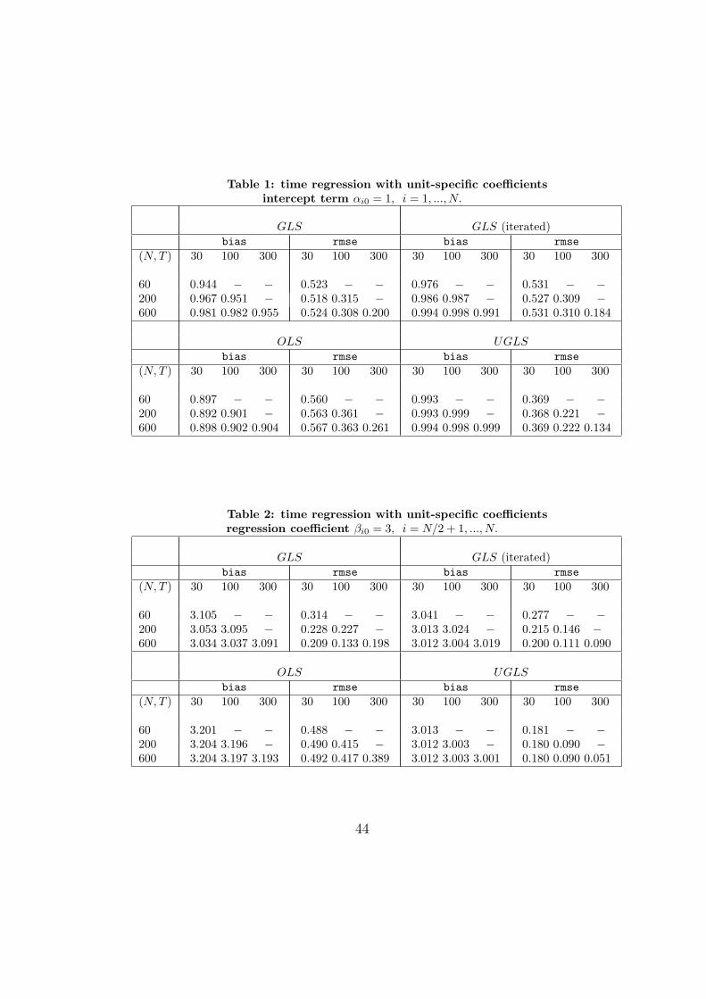
Table 1: time regression with unit-specific coefficientsintercept term αi0 = 1, i = 1, ..., N.

GLS GLS (iterated)bias rmse bias rmse

(N, T ) 30 100 300 30 100 300 30 100 300 30 100 300

60 0.944 − − 0.523 − − 0.976 − − 0.531 − −200 0.967 0.951 − 0.518 0.315 − 0.986 0.987 − 0.527 0.309 −600 0.981 0.982 0.955 0.524 0.308 0.200 0.994 0.998 0.991 0.531 0.310 0.184

OLS UGLSbias rmse bias rmse

(N, T ) 30 100 300 30 100 300 30 100 300 30 100 300

60 0.897 − − 0.560 − − 0.993 − − 0.369 − −200 0.892 0.901 − 0.563 0.361 − 0.993 0.999 − 0.368 0.221 −600 0.898 0.902 0.904 0.567 0.363 0.261 0.994 0.998 0.999 0.369 0.222 0.134

Table 2: time regression with unit-specific coefficientsregression coefficient βi0 = 3, i = N/2 + 1, ..., N.

GLS GLS (iterated)bias rmse bias rmse

(N, T ) 30 100 300 30 100 300 30 100 300 30 100 300

60 3.105 − − 0.314 − − 3.041 − − 0.277 − −200 3.053 3.095 − 0.228 0.227 − 3.013 3.024 − 0.215 0.146 −600 3.034 3.037 3.091 0.209 0.133 0.198 3.012 3.004 3.019 0.200 0.111 0.090

OLS UGLSbias rmse bias rmse

(N, T ) 30 100 300 30 100 300 30 100 300 30 100 300

60 3.201 − − 0.488 − − 3.013 − − 0.181 − −200 3.204 3.196 − 0.490 0.415 − 3.012 3.003 − 0.180 0.090 −600 3.204 3.197 3.193 0.492 0.417 0.389 3.012 3.003 3.001 0.180 0.090 0.051

44

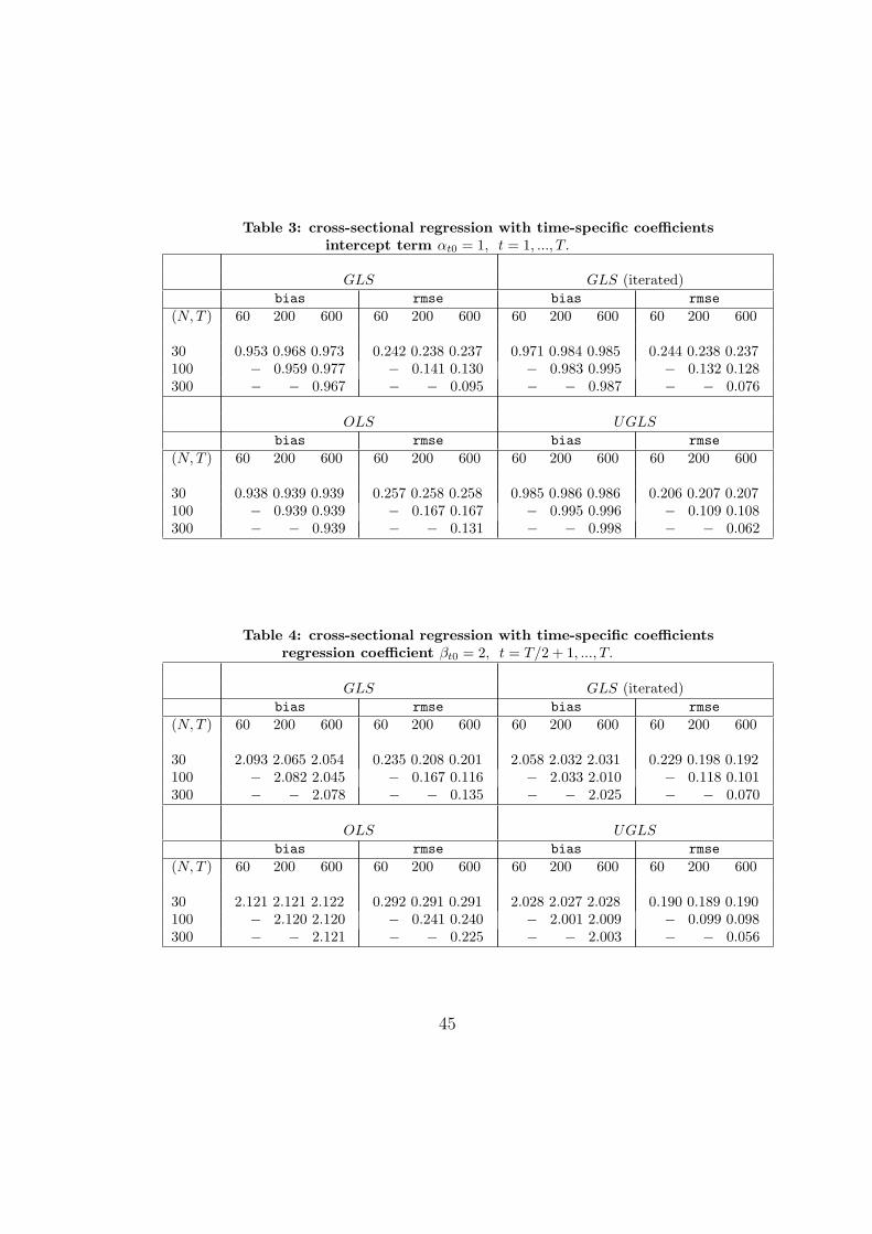
Table 3: cross-sectional regression with time-specific coefficientsintercept term αt0 = 1, t = 1, ..., T.

GLS GLS (iterated)bias rmse bias rmse

(N, T ) 60 200 600 60 200 600 60 200 600 60 200 600

30 0.953 0.968 0.973 0.242 0.238 0.237 0.971 0.984 0.985 0.244 0.238 0.237100 − 0.959 0.977 − 0.141 0.130 − 0.983 0.995 − 0.132 0.128300 − − 0.967 − − 0.095 − − 0.987 − − 0.076

OLS UGLSbias rmse bias rmse

(N, T ) 60 200 600 60 200 600 60 200 600 60 200 600

30 0.938 0.939 0.939 0.257 0.258 0.258 0.985 0.986 0.986 0.206 0.207 0.207100 − 0.939 0.939 − 0.167 0.167 − 0.995 0.996 − 0.109 0.108300 − − 0.939 − − 0.131 − − 0.998 − − 0.062

Table 4: cross-sectional regression with time-specific coefficientsregression coefficient βt0 = 2, t = T/2 + 1, ..., T.

GLS GLS (iterated)bias rmse bias rmse

(N, T ) 60 200 600 60 200 600 60 200 600 60 200 600

30 2.093 2.065 2.054 0.235 0.208 0.201 2.058 2.032 2.031 0.229 0.198 0.192100 − 2.082 2.045 − 0.167 0.116 − 2.033 2.010 − 0.118 0.101300 − − 2.078 − − 0.135 − − 2.025 − − 0.070

OLS UGLSbias rmse bias rmse

(N, T ) 60 200 600 60 200 600 60 200 600 60 200 600

30 2.121 2.121 2.122 0.292 0.291 0.291 2.028 2.027 2.028 0.190 0.189 0.190100 − 2.120 2.120 − 0.241 0.240 − 2.001 2.009 − 0.099 0.098300 − − 2.121 − − 0.225 − − 2.003 − − 0.056

45

References

Ahn, S. C., Y. Hoon Lee, and P. Schmidt (2001): “GMM estimationof linear panel data models with time-varying individual effects,” Journalof Econometrics, 101, 219–255.

Andrews, D. (2005): “Cross-section regression with common shocks,”Econometrica, 73, 1551–1585.

Anselin, L. (1988): Spatial econometrics: methods and models. Dordrecht:Kluwer Academic Publishers.

Bai, J. (2003): “Inferential theory for factor models of large dimensions,”Econometrica, 71, 135–171.

Bai, J., and S. Ng (2002): “Determining the number of factors in approx-imate factor models,” Econometrica, 70, 191–221.

Bai, J., and S. Ng (2004): “A PANIC attack on unit roots and cointegra-tion,” Econometrica, 72, 1127–1177.

Brown, B. M. (1971): “Martingale central limit theorems,” Annals ofMathematical Statistics, 42, 59–66.

Case, A. C. (1991): “Spatial patterns in household demand,” Economet-rica, 59, 953–965.

Chamberlain, G. (1983): “Funds, factors, and diversification in arbitragepricing models,” Econometrica, 51, 1305–1323.

Chen, X., and T. G. Conley (2001): “A new semiparametric spatialmodel for panel time series,” Journal of Econometrics, 105, 59–83.

Conley, T. G. (1999): “GMM estimation with cross sectional dependence,”Journal of Econometrics, 92, 1–45.

Forni, M., M. Hallin, M. Lippi, and R. L. (2000): “The generalizeddynamic-factor model: identification and estimation,” The Review of Eco-nomics and Statistics, 82, 540–554.

46

Hallin, M., and R. Liska (2007): “Determining the number of factorsin the general dynamic factor model,” Journal of the American StatisticalAssociation, 102, 603–617.

Holtz-Eakin, D., W. Newey, and H. S. Rosen (1988): “Estimatingvector autoregressions with panel data,” Econometrica, 56, 1371–95.

Lee, L. F. (2004): “Asymptotic distributions of quasi-maximum likelihoodestimators for spatial autoregressive models,” Econometrica, 72, 1899–1925.

Magnus, J. R., and H. Neudecker (1988): Matrix Differential Calculuswith Applications in Statistics and Econometrics, Probability & Mathe-matical Statistics. London: John Wiley & Sons.

Moon, H. R., and B. Perron (2003): “Testing for a unit root in panelswith dynamic factors,” Journal of Econometrics.

Pesaran, M. H. (2006): “Estimation and inference in large heterogeneouspanels with a multifactor error structure,” Econometrica, 74, 967–1012.

Pesaran, M. H., and E. Tosetti (2007): “Large panels with commonfactors and spatial correlations,” IZA Discussion Paper n. 3032.

Pesaran, M. H., and P. Zaffaroni (2008): “Optimal asset allocationwith factor models for large portfolios,” Imperial College London, preprint.

Phillips, P. C. B., and D. Sul (2003): “Dynamic panel estimation andhomogeneity testing under cross section dependence,” Econometrics Jour-nal.

(2007): “Bias in dynamic panel estimation with fixed effects, in-cidental trends and cross section dependence,” Journal of Econometrics,137, 162–188.

Robinson, P. M. (2006): “Efficient estimation of the semiparametric spa-tial autoregressive model,” Journal of Econometrics forthcoming.

Robinson, P. M., and F. J. Hidalgo (1997): “Time series regressionwith long-range dependence,” Annals of Statistics, 25, 77–104.

47

Stock, J. H., and M. W. Watson (2002): “Macroeconomic forecastingusing diffusion indexes,” Journal of Business & Economic Statistics, 20,147–62.

48