Generalized Global Bandit and Its Application in Cellular

218 IEEE JOURNAL OF SELECTED TOPICS IN SIGNAL PROCESSING, VOL. 12, NO. 1, FEBRUARY 2018

Generalized Global Bandit and Its Application inCellular Coverage Optimization

Cong Shen , Senior Member, IEEE, Ruida Zhou, Cem Tekin , Member, IEEE,and Mihaela van der Schaar, Fellow, IEEE

Abstract—Motivated by the engineering problem of cellular cov-erage optimization, we propose a novel multiarmed bandit modelcalled generalized global bandit. We develop a series of greedyalgorithms that have the capability to handle nonmonotonic butdecomposable reward functions, multidimensional global param-eters, and switching costs. The proposed algorithms are rigorouslyanalyzed under the multiarmed bandit framework, where we showthat they achieve bounded regret, and hence, they are guaranteed toconverge to the optimal arm in finite time. The algorithms are thenapplied to the cellular coverage optimization problem to achievethe optimal tradeoff between sufficient small cell coverage andlimited macroleakage without prior knowledge of the deploymentenvironment. The performance advantage of the new algorithmsover existing bandits solutions is revealed analytically and furtherconfirmed via numerical simulations. The key element behind theperformance improvement is a more efficient “trial and error”mechanism, in which any trial will help improve the knowledge ofall candidate power levels.

Index Terms—Multi-armed bandit, online learning, regret anal-ysis, coverage optimization.

I. INTRODUCTION

R ECENT years have witnessed a significant growth of smallbase stations (SBS), such as pico and femto, that are mas-

sively deployed to address the capacity and coverage challengeof wireless networks [1]. In practice, SBSs may be deployedin drastically different scenarios, with different target coverage

Manuscript received July 14, 2017; revised October 30, 2017; accepted Jan-uary 15, 2018. Date of publication January 25, 2018; date of current versionFebruary 16, 2018. The work of C. Shen and R. Zhou was supported by theNational Natural Science Foundation of China under Grant 61572455 and Grant61631017. The work of C. Tekin was supported by the Scientific and Techno-logical Research Council of Turkey (TUBITAK) under 3501 Program Grant116E229. The work of M. van der Schaar was supported by the National Sci-ence Foundation under Grant 1407712 and Grant 1533983. The guest editorcoordinating the review of this paper and approving it for publication was Prof.H. Vincent Poor. (Corresponding author: Cong Shen.)

C. Shen and R. Zhou are with the School of Information Science and Tech-nology, University of Science and Technology of China, Hefei 230027, China(e-mail: [email protected]; [email protected]).

C. Tekin is with the Department of Electrical and Electronics Engineer-ing, Bilkent University, Ankara 06800, Turkey (e-mail: [email protected]).

M. van der Schaar is with the Oxford-Man Institute of Quantitative Fi-nance (OMI) and the Department of Engineering Science, University of Oxford,Oxford OX1 2JD, U.K., and also with the Electrical Engineering Department,University of California, Los Angeles (UCLA), Los Angeles, CA 90095 USA(e-mail: [email protected]).

Color versions of one or more of the figures in this paper are available onlineat http://ieeexplore.ieee.org.

Digital Object Identifier 10.1109/JSTSP.2018.2798164

objectives. In addition, the radio frequency (RF) conditions mayvary significantly from one deployment to another. Due to theheterogeneous nature of these deployments, setting an appro-priate transmit power of each deployed SBS, which effectivelydetermines the coverage, becomes an important task that mustbe decided based on the specific deployment scenario. If thetransmit power is too small, the resulting coverage may notsufficiently cover the intended area. On the other hand, if thetransmit power is too large, the SBS coverage will leak intomacrocells and cause unnecessary interference, especially if theSBS operates in a close-access mode.

Traditional approaches to cell coverage optimization rely onRF engineers to carry out on-the-spot field measurements to ef-fectively “learn” the specific deployment environment, and op-timize the coverage and leakage using RF planning tools. Thisapproach, however, becomes increasingly infeasible for SBS de-ployment as it does not scale with the significant increase of net-work nodes (high density), multiple layers of nodes (heterogene-ity), and multiple radio access technologies (3G/4G/Wifi) [2].Furthermore, non-stationarity of the environment, such as dy-namic user behavior and RF footprint variations, may cause thepreviously optimal configuration to become highly sub-optimaland lead to performance degradation [3].

Applying online learning algorithms to cellular coverageoptimization is an important means to address the aforemen-tioned challenges, as they allow for adaptive, automated andautonomous coverage adjustment while minimizing the plannedhuman involvement. A good coverage learning solution has tobalance the immediate gains (selecting a coverage that is thebest based on current knowledge) and long-term performance(evaluating other coverage levels). We thus resort to the the-ory of multi-armed bandit (MAB) [4] to address the resultingexploration and exploitation tradeoff. It is worth noting thatMAB-inspired algorithms have been adopted in various othersimilar tasks, such as power calibration [5], mobility manage-ment [6]–[8], and channel selection [9].

However, a direct application of standard MAB algorithms(such as UCB [10]1) to the coverage optimization problem, al-beit feasible, ignores the inherent structure and hence cannotfully exploit the characteristics of the underlying communica-tion model. First, unlike the standard MAB model where dif-ferent arms are independent, coverage performances of similartransmit power levels are often very similar, which means that

1Throughout this paper, UCB specifically refers to UCB1 in [10].

1932-4553 © 2018 IEEE. Personal use is permitted, but republication/redistribution requires IEEE permission.See http://www.ieee.org/publications standards/publications/rights/index.html for more information.

https://orcid.org/0000-0002-3148-4453

https://orcid.org/0000-0003-4361-4021

SHEN et al.: GENERALIZED GLOBAL BANDIT AND ITS APPLICATION IN CELLULAR COVERAGE OPTIMIZATION 219

if we adopt the MAB model, nearby arms are highly correlated.Intuitively, such correlation can be used to accelerate the con-vergence to the optimal selection, because any sampling of onearm not only reveals information about itself, but also nearbyarms that are highly correlated. Second, the correlated coverageperformance of different power levels fundamentally originatesfrom the fact that they all follow the same physical RF propa-gation law, which has been captured in various standard models(e.g., 3GPP model [11]).

In this work, motivated by this engineering problem, we firstpropose a novel MAB model, called Generalized Global Bandit(GGB), that is a non-trivial extension of Global Bandit (GB) in[12], [13]. In GB, the expected reward of each arm is a (possiblynon-linear) function of a single parameter, and different armsare correlated through this global parameter. Furthermore, thisfunction is required to be monotonic. As we will see, the orig-inal GB model and the resulting algorithms cannot be directlyapplied to coverage optimization due to three unique features.First, cellular coverage optimization needs to balance sufficientcoverage within the intended area and limited leakage to out-side macro users. As a result, the reward function will not bemonotonic.2 Second, the reward function may have multipleunknown parameters. The GB model in [12], however, cannotbe trivially extended to handle more than one global parameter.Lastly, a practical coverage optimization solution needs to avoidfrequent power changes, as it may cause frequent variation of thecoverage area and result in uneven user experience. Hence, thesolution should explicitly consider switching cost to discouragefrequent changes to the coverage area.

We address these three new challenges in the GGB model.The reward function of each arm is allowed to be non-monotonicbut decomposable, which fits well with the considered cover-age optimization problem. Multi-dimensional global parametersand switching cost are also considered in the GGB model. Wethen present the ad-greedy policy, which can simultaneouslymaximize the accumulated rewards and estimate the unknownparameters via an updated weight average on different arms.Rigorous regret analysis is carried out for the proposed policyand its variants, where we show that bounded regret is achiev-able, and hence, the policy is guaranteed to converge to theoptimal arm in finite time. In other words, the one-step regretapproaches zero asymptotically. The algorithms are then appliedto the cell coverage optimization problem to achieve the opti-mal tradeoff between sufficient SBS coverage and limited macroleakage without prior knowledge of the deployment. Numericalsimulation results are provided to demonstrate the performanceadvantage of the new algorithms over the existing bandit solu-tions.

The main contributions of this work are summarized as fol-lows.

� Motivated by the practical constraints of the cellular cov-erage optimization problem, we propose a generalizedglobal bandit model, which can handle non-monotonic but

2It is worth noting that the monotonicity requirement is fundamental to theWAGP algorithm in [12], which is one of the two key assumptions in [12,Sec. III].

decomposable reward functions, multi-dimensional globalparameters, and switching costs.

� We develop the ad-greedy policy for the considered GGBmodel, and rigorously analyze its regret. We show that the(total) regret is bounded, and hence, the one-step regretdiminishes asymptotically.

� We apply the GGB model and the ad-greedy policy andits variants to the cellular coverage optimization problem,and illustrate how the proposed variants fit to this engi-neering problem. We further verify the advantages of thenew algorithms via numerical simulations. Furthermore,we also numerically evaluate the algorithm performancein a non-stationary environment, when the MBS signalstrength slowly changes over time.

The rest of the paper is organized as follows. Related liter-ature is discussed in Section II. The GGB formulation, the ad-greedy policies, and the corresponding regret analysis are givenin Section III. In Section IV, we describe how the GGB modelcan be applied to the cellular coverage optimization problem,and present the numerical simulation results. Finally, Section Vconcludes the paper.

II. RELATED WORK

A. MAB With Arm Correlations

MAB is a powerful tool to model sequential decision prob-lems with an intrinsic exploration-exploitation tradeoff. In theclassic stochastic MAB model, each arm, if played, generatesan instantaneous reward that is independently and identically(i.i.d.) drawn from a fixed distribution, which is unknown to theforecaster a priori. The design objective is to maximize the totalexpected reward accumulated through a sequence of T plays,which can be equivalently formulated as to minimize the regretbetween the total expected reward from always playing the armwith the highest expected reward and that from the learningalgorithm.

The fundamental regret lower bound for stochastic MAB wasdeveloped by Lai and Robbins in [14], and a matching upperbound is achieved by the celebrated Upper Confidence Bound(UCB) algorithm [10]. Using UCB, at each round the playersimply pulls the arm that has the highest sample mean rewardplus an uncertainty term that is inversely proportional to thenumber of times the arm has been played. There is a rich body ofliterature on MABs, which we will not survey comprehensively.Interested readers are referred to [4] and the references therein.

In the MAB literature, the most relevant work to our GGBmodel is the study on MAB with arm correlations. Existing re-search on this topic can be divided into two categories: Bayesianmodel [15], [16] and parameterized model [17]–[19]. In theBayesian model, arm correlation is captured by stochastic mea-sures such as mean and covariance matrix. This approach and thecorresponding bandit algorithms have been studied in [15], [16].The authors of [15] propose bandit algorithms with a Bayesianprior on the mean reward that is based on a human decision-making model. The authors of [16] further extend the algorithmto focus on the correlation among arms. Linear bandit [17] isa primary example of the parameterized model, in which the


expected reward of each arm is a linear function of a global pa-rameter. For this model, [18] proves a regret bound that scaleslinearly with the dimension of the parameter. The authors of[19] establish a lower bound for an arbitrary policy for themulti-dimensional linear bandit, and then provide a matchingupper bound through a policy that alternates between explo-ration and exploitation. The GGB setting is more general thanthese above models as it allows for non-linear non-monotonicreward functions with multi-dimensional parameters. For thespecial case when the expected sub-function rewards are all lin-ear in multi-dimensional parameters, our setting reduces to thelinear bandit model.

B. Non-Linear Parameter Estimation

Another line of relevant work is in the area of non-linearparameter estimation [20]–[22]. In [21], the author studies thenon-linear parameter estimation problem with additive Gaussiannoise. The authors of [20] prove that the nonlinear least-squareestimator is able to asymptotically attain the Cramer-Rao lowerbound under additive Gaussian noise, even when there is a mis-match of noise distribution. The authors of [22] focus on theimpact of compressed sensing on Fisher information and theCramer-Rao bound. The main difference to our work is thatthese papers do not need to consider the exploration and ex-ploitation tradeoff that is fundamental to the MAB problems.They only care about estimating the parameter as accurately aspossible, while we aim at maximizing the long-term reward ofa bandit policy.

C. Cellular Coverage Optimization

Coverage optimization is an important task in cellular net-work deployment. Under the self-organizing networking (SON)framework, this task is captured in the Capacity and CoverageOptimization (CCO) feature, which is part of the 3GPP SONdeliverables [23]. In practice, coverage optimization has beenimplemented and deployed in commercial SON products suchas Cisco SON [24] and Qualcomm UltraSON [25]. In academia,coverage optimization is an active research topic [26], [27]. Ex-isting studies have focused on optimizing different system pa-rameters, such as antenna tilt [28]–[30], and downlink transmitpower [5], [31], [32].

In [28], the impact of half-power beamwidths and downtiltantenna angle to the overall network performance is studied. Acell coverage optimization problem for uplink massive MIMO isstudied in [29], which is based on optimizing the tilt-adjustableantennas at SBS. A general framework incorporating both down-link and uplink coverage, while requiring very sparse systemknowledge, is proposed in [30].

Besides antenna parameter optimization, another line of studyfocuses on adjusting the SBS transmit power so that the result-ing coverage balances maximizing intended coverage and min-imizing undesirable leakage. Our application of coverage opti-mization also falls into this category. Claussen et al. [31] haveproposed a method that uses information on mobility events ofoutdoor and indoor users to optimize the transmit power. Thisapproach is further enhanced in [32], where a systematic study

of indoor enterprise SBS networks is carried out. Both of theseworks require knowledge of the deployment, such as intendedarea and co-channel macrocell footprint, which is not assumedin this work. Alternatively, adjusting the SBS transmit powerwithout deployment knowledge has recently been consideredin [5], where the MAB model is applied and the correlationof different power levels is captured using a Bayesian frame-work. However, it does not fully utilize the available structuralinformation of the system.

III. GENERALIZED GLOBAL BANDIT MODEL AND

GREEDY POLICIES

In this section, we first present the common baseline formu-lation, and then discuss three generalizations to the underlyingmodel: non-monotonic decomposable reward functions, multi-dimensional global parameters, and switching costs. For eachof these generalizations, we will present the greedy policies andanalyze their regrets.

A. The Baseline GGB Formulation

We consider a stochastic MAB formulation with K arms,indexed by K = {1, . . . , K}. A forecaster can choose and playexactly one arm at each time slot. Arm k ∈ K, if played, willoffer a bounded reward that is drawn from a distribution νk

with a finite support, and we denote its mean as μk . We useXk,t to denote the random reward of arm k at time slot t,which is independently drawn from other arms. Without lossof generality, we assume that the rewards are bounded withinthe unit interval [0, 1]. The forecaster has no prior knowledge ofeither νk or μk , ∀k ∈ K. The forecaster’s goal is to design anarm selection policy that maximizes the total reward it obtainsover time.

Within the framework of global bandits [12], there exists aglobal parameter θ∗, which is associated to the expected rewardsof all arms μk = μk (θ∗) = Eνk

[Xk,t ], where Eνk[·] denotes

expectation with respect to distribution νk . The parameter θ∗,unknown to the forecaster, belongs to a parameter set Θ, whichagain is normalized to be the unit interval for simplicity.

The forecaster knows the reward function μk (θ) for eachk ∈ K, but not the true global parameter θ∗. At each time slot,the forecaster only observes the random reward from the cho-sen arm, and her goal is to maximize the cumulative rewardup to any given time T . Obviously, if the global parameter isperfectly known to the forecaster, she will always select the opti-mal arm k∗(θ∗) = arg maxk∈K μk (θ∗), with the correspondingoptimal expected reward μ∗(θ∗) = maxk∈K μk (θ∗). When θ∗ isclear from the context, we use k∗ and μ∗ instead of k∗(θ∗) andμ∗(θ∗). For simplicity of exposition and without loss of general-ity, throughout the paper it is assumed that there exists a uniquebest arm for θ∗. We define the one-step (pseudo) regret at time tas rIt

(θ∗).= μ∗(θ∗) − μIt

(θ∗), where It is the selected arm bythe forecaster’s policy at time t. The total regret [4] by time Tis given as

Reg(T ) = E

[T∑

t=1

rIt(θ∗)

]. (1)


B. Non-Monotonic Decomposable Reward Functions

1) Model and Algorithm: A significant constraint of [12] isthat μk (θ) must be an invertible function of θ. Hence the rewardfunction must be monotonic. If the monotonicity condition istotally removed, the GB problem becomes difficult to study. Ourapproach in this work, nevertheless, is to exploit the structureof the cellular coverage optimization problem and relax themonotonicity constraint to a certain degree such that it not onlyfits our problem setting but also is tractable.

Fortunately, for the cellular coverage optimization problem,the objective function is generally defined as a linear combina-tion of two (or more) conflicting functions (see [5, eq. (3)] for anexample). As a result, the overall function is not monotonic withrespect to θ, but the individual sub-functions are, and they aremonotonic in the opposite direction. For instance, the specificPerformance Indication Function (PIF) fk (θ) of [5] (equivalentto the expected reward function μk (θ) in GB), can be decom-posed into the linear combination of two sub-functions. One ofthem denotes the coverage, which increases monotonically withthe coverage radius d, while the other one denotes the leakage,which decreases monotonically with d.

Formally, the expected reward function μk (θ) can be decom-posed into J continuous sub-functions:

μk (θ) =J∑

j=1

αjμj,k (θ). (2)

These sub-functions and their weights are assumed to beknown to the forecaster, but not the true parameter θ∗. Foreach j ∈ J = {1, . . . , J} and k ∈ K = {1, . . . , K}, the sub-function μj,k (θ) satisfies the Holder continuity and monotonic-ity assumptions as [12, Assumption 1]. More specifically, thefollowing assumptions are made.

Assumption 1:1) (Holder continuity) For each j ∈ J , k ∈ K and θ, θ′ ∈

Θ, there exists D2,j,k > 0 and 0 < γ2,j,k ≤ 1, such that:

|μj,k (θ) − μj,k (θ′)| ≤ D2,j,k |θ − θ′|γ2 , j , k . (3)

2) (Sub-function monotonicity) For each j ∈ J , k ∈ K andθ, θ′ ∈ Θ, there exists D1,j,k > 0 and 1 < γ1,j,k , suchthat:

|μj,k (θ) − μj,k (θ′)| ≥ D1,j,k |θ − θ′|γ1 , j , k . (4)

We want to emphasize that Assumption 1 is mild. For theapplication of cellular coverage optimization, the sub-functionmonotonicity has been discussed, and the Holder continuitycondition can also be met when the coverage/leakage functionchanges smoothly with the intended coverage area. This pointwill become more clear when we discuss the application of GGBto the cellular coverage problem in Section IV.

We further assume that whenever an arm k is played, the fore-caster receives the sub-function reward realizations {Xj

k,t}j∈J .Sub-function reward realizations are independent between arms,and i.i.d. over time. Receiving {Xj

k,t}j∈J is a reasonable as-sumption for some practical scenarios, such as the consideredcoverage optimization problem where the coverage events are

reported by SBS users through the measurement reports and mo-bility protocols, and the leakage events are reported by macrousers through registration attempts, respectively. Such approachhas been adopted in previous papers, e.g., [32], [33], and hasbeen successfully adopted in practical transmit power assign-ment solution, e.g., [25].

With Assumption 1, we have the following proposition.Proposition 1: Define

D2 = max{D2,j,k |j ∈ J , k ∈ K},γ1 = max{γ1,j,k |j ∈ J , k ∈ K},γ2 = min{γ2,j,k |j ∈ J , k ∈ K},

μj,k

= minθ∈Θ

μj,k (θ), μj,k = maxθ∈Θ

μj,k (θ)

and

γ1 =1γ1

,

D1 = max

{(1

D1,j,k

) 1γ 1 , j , k |j ∈ J , k ∈ K

}.

The following statements hold:1) For each j ∈ J , k ∈ K and θ, θ′ ∈ Θ,

|μj,k (θ) − μj,k (θ′)| ≤ D2 |θ − θ′|γ2 . (5)

2) For each j ∈ J , k ∈ K and y, y′ ∈ [μj,k

, μj,k ],

|μ−1j,k (y) − μ−1

j,k (y′)| ≤ D1 |y − y′|γ1 . (6)

Proof: Inequality (5) is a direct application of (3) ofAssumption 1 and the definitions of D2 and γ2 . For the proofof inequality (6), we first note that the reward sub-functionsare invertible due to the sub-function monotonicity part ofAssumption 1. Then, inequality (6) is directly obtained by plug-ging the inverse functions in (4) and applying the definitions ofγ1 and D1 . �

We present a greedy policy, called the ad-greedy policy, whichcan effectively handle non-monotonic decomposable rewardfunctions. The pseudocode of the ad-greedy policy is givenin Algorithm 1.

As the name suggests, the ad-greedy policy is a greedy pro-cedure at its core, with the capability to adaptively update theparameter estimate using all the observed reward realizationsfrom sub-functions. Other than the initial time slot where noprior information is available, where an arm I1 is uniformlychosen among all arms, the arm selection always chooses It

with the highest estimated reward:

It = arg maxk∈K

μk (θt−1).

This is the same as the greedy policy for classic MAB problems,which is well-known [4], [10] to be strictly sub-optimal andcannot achieve log(t) order of regret. However, as we will seelater in the regret analysis, this simple greedy policy sufficesto achieve bounded regret in our GGB model due to the globalinformativeness.

In addition to the greedy arm selection, the policy also car-ries out an update on the global parameter estimation using


estimates from individual sub-functions of individual arms, andweighing them differently. The weights are updated accordingto the number of times the arm is played.

2) Regret Analysis: The optimality region Θk for any arm kis defined as

Θk = {θ ∈ Θ|k ∈ k∗(θ)} . (7)

We then define δ as the smallest Euclidean distance between θ∗and the boundary of Θk ∗ . Since there is a unique best arm forθ∗ and since the reward functions are continuous in θ, we haveδ > 0. The total regret up to time T can be written as the sumof one-step regrets Reg(T ) = E[

∑Tt=1 rIt

(θ∗)]. Thanks to thenormalization, the one-step regret for t > 1 can be bounded by

E[rIt(θ∗)] ≤ 1 · Pr {It �= k∗(θ∗)} = Pr

{θt−1 ∈ Θ\Θk ∗

}.

Theorem 1: The regret of the ad-greedy policy for a finitetime horizon T is upper bounded by

Reg(T ) ≤ 1 + 2JKe−α − Te−αT + (T − 1)e−α(T +1)

(1 − e−α )2 ,

where α = 2( δK D1

)2γ1 > 0. Furthermore, the infinite time hori-zon regret of the ad-greedy policy is finite, i.e.,

Reg(∞) ≤ 1 + 2JKe−α

(1 − e−α )2 .

Proof: Before deriving a bound of the gap between the pa-rameter estimate at time slot t and the true parameter, welet μ−1

j,k (y) .= arg minθ∈Θ |μj,k (θ) − y| for y ∈ [0, 1]. By themonotonicity of μj,k (·) and Proposition 1, we have |μ−1

j,k (y) −

μ−1j,k (y′)| ≤ D1 |y − y′|γ1 for all y, y′ ∈ [0, 1]. Then, we have

|θt − θ∗|

=

∣∣∣∣∣∑k∈K

ωk (t)

∑j∈J θj

k ,t

J− θ∗

∣∣∣∣∣≤ 1

J

∑j∈J

∑k∈K

∣∣∣ωk (t)θjk ,t − ωk (t)θ∗

∣∣∣≤ 1

J

∑j∈J

∑k∈K

ωk (t)∣∣∣μ−1

j,k (Xjk,t) − μ−1

j,k (μj,k (θ∗))∣∣∣

≤ 1J

∑j∈J

∑k∈K

ωk (t)D1 |Xjk,t − μj,k (θ∗)|γ1 .

Next, we analyze the event that the gap |θt − θ∗| is no smallerthan δ. Note that when the gap is smaller than δ, It+1 = k∗. Thismay not hold when the gap is larger than or equal to δ.

{δ ≤ |θt − θ∗|

}

⊂⎧⎨⎩δ ≤ 1

J

∑j∈J

∑k∈K

ωk (t)D1 |Xjk,t − μj,k (θ∗)|γ1

⎫⎬⎭

=

⎧⎨⎩∑j∈J

∑k∈K

δ

JK≤∑j∈J

∑k∈K

ωk (t)D1

J|Xj

k,t − μj,k (θ∗)|γ1

⎫⎬⎭

⊂⋃k∈K

⋃j∈J

{δ

JK≤ ωk (t)D1

J|Xj

k,t − μj,k (θ∗)|γ1

}

=⋃k∈K

⋃j∈J

{(δ

KD1ωk (t)

)γ1

≤ |Xjk,t − μj,k (θ∗)|

}. (8)

Define Xjk,s as the empirical mean of the first s observations of

sub-reward j of arm k, which are i.i.d. based on the assumptionthat sub-rewards of the same arm are i.i.d. over time. The one-step regret is bounded as follows:

Pr {It+1 �= k∗} = Pr{

θt ∈ Θ\Θk ∗}

≤ Pr{

δ ≤ |θt − θ∗|}

(a)≤∑j∈J

∑k∈K

Pr

{( δ

KD1ωk (t)

)γ1 ≤ |Xjk,t − μj,k (θ∗)|

}

=∑j∈J

∑k∈K

E[1{( δt

KD1Nk (t)

)γ1 ≤ |Xjk,t − μj,k (θ∗)|

}]

(b)≤∑j∈J

∑k∈K

E

[1

{∃s ∈ {1, 2, . . . , t},

(δt

KD1s

)γ1

≤ |Xjk,s − μj,k (θ∗)|

}]


(c)≤∑j∈J

∑k∈K

t∑s=1

E

[1

{(δt

KD1s

)γ1

≤ |Xjk,s − μj,k (θ∗)|

}]

(d)≤∑j∈J

∑k∈K

t∑s=1

2

[exp

(−2(

δt

KD1s

)2γ1

s

)]

= 2JK

t∑s=1

[exp

(−2(

δ

KD1

)2γ1 (s

t

)1−2γ1

t

)]

(e)≤ 2JKt exp

(−2(

δ

KD1

)2γ1

t

), (9)

where (a) is from (8) and the union bound, (b) follows from thefact that{

(δt

KD1Nk (t))γ1 ≤ |Xj

k,t − μj,k (θ∗)|}

⊂{∃s ∈ {1, 2, . . . , t},

(δt

KD1s

)γ1

≤ |Xjk,s − μj,k (θ∗)|

},

(c) is again from the union bound, (d) is obtained via Hoeffding’sinequality, and (e) is based on the fact that

(st

)1−2γ1 ≥ 1, whichis true by Assumption 1 and Proposition 1.

Finally, with the one-step regret bound (9), the total regretReg(T ) can be bounded by summing (9) over t = 1, . . . , T asfollows:

Reg(T ) ≤T∑

t=1

Pr {It �= k∗(θ∗)}

≤ 1 +T −1∑t=1

2JKt exp(− 2(

δ

KD1)2γ1 t)

= 1 + 2JKe−α − Te−αT + (T − 1)e−α(T +1)

(1 − e−α )2 .

Letting T go to infinity gives

Reg(∞) ≤ 1 + 2JKe−α

(1 − e−α )2 .

�Theorem 1 is important as it states that the regret of the ad-

greedy policy is bounded. This also implies that the ad-greedypolicy converges to the optimal arm k∗ with probability one.

C. Multi-Dimensional Global Parameters

1) Model and Algorithm: The model in Section III-B andthe original GB model of [12] only consider a scalar parameterθ. In this section, the GB model and the ad-greedy policy areextended to the multi-dimensional case for �θ. In reality, practicalproblems often have multiple parameters that affect the systemperformance. For example, cellular coverage optimization is de-pendent on many environmental variables, such as deploymentarea, macrocell footprints, target SINR, etc.

Increasing the parameter dimension brings non-trivial tech-nical difficulty to the GGB model. To highlight the contributionand for the ease of illustration, we study the case where the

global parameter is 2-dimensional. Extensions to higher dimen-sions can be done with the same philosophy, but the resultinganalysis is much more complicated. Furthermore, we note thatthis section still considers the non-monotonic reward functionsas in Section III-B.

To accommodate for the vector form of GGB, we re-definesome of the previous notations and introduce new notations.

� �θ∗ = [θ1∗, θ2∗] denotes the true unknown 2-dimensionalglobal parameter. �θ = [θ1 , θ2 ] ∈ Θ denotes any parametervector that is in the parameter set Θ. We normalize Θ suchthat ||�θ − �θ′|| ≤ 1 for any �θ, �θ′ ∈ Θ, where || · || denotesthe Euclidean norm.

� k∗ = k∗(�θ∗) denotes the true best arm. k∗(�θ) denotes theset of best arm(s) when the global parameter is �θ.

� Θk = {�θ ∈ Θ|k∈k∗(�θ)}.� δ is the Euclidean distance between �θ∗ and the boundary

of Θk ∗ .� μk (�θ) ∈ [0, 1] is the reward function that is composed of

J sub-functions:

μk (�θ) =J∑

j=1

αjμj,k (�θ).

� Ψj,k (X) ⊂ Θ, is the contour of μj,k (�θ) to X , i.e.,

Ψj,k (X) ={

�θ ∈ Θ|μj,k (�θ) = X}

. (10)

Furthermore, the following assumptions are imposed for themulti-dimensional GGB problem.

Assumption 2:1) J ≥ 2.2) For �θ∗ ∈ Θ and k ∈ K, there exists a J-dimensional

cube with center (μ1,k (�θ∗), μ2,k (�θ∗), . . . , μJ,k (�θ∗)) andthe edge length 2λk (�θ∗) such that, for any j, j′ ∈ J ,j �= j′, X ∈ [μj,k (�θ∗) − λk (�θ∗), μj,k (�θ∗) + λk (�θ∗)], andX ′ ∈ [μj ′,k (�θ∗) − λk (�θ∗), μj ′,k (�θ∗) + λk (�θ∗)], two con-tours Ψj,k (X) and Ψj ′,k (X ′) have exactly one intersec-tion. Denote λ = mink∈K(λk (�θ∗)).

3) For j, j′ ∈ J , j′ �= j, k ∈ K, and �θ, �θ′ ∈ Ψj,k (X),there exists D1,j,j ′,k ,X > 0 and 0 < γ1,j,j ′,k ,X ≤ 1,D2,j,j ′,k ,X > 0 and 1 < γ2,j,j ′,k ,X , such that:

|μj ′,k (�θ) − μj ′,k (�θ′)| ≥ D1,j,j ′,k ,X ||�θ − �θ′||γ1 , j , j ′ , k , X

j,k ,X

|μj ′,k (�θ) − μj ′,k (�θ′)| ≤ D2,j,j ′,k ,X ||�θ − �θ′||γ2 , j , j ′ , k , X

j,k ,X

where ||�θ − �θ′||j,k ,X is the rectification of contour Ψj,k (X)between �θ and �θ′.

The first assumption is made so that the forecaster can esti-mate �θ∗ by using pairs of Ψj,l(X

jl,t), j ∈ J sets at each play.

The second assumption guarantees that as the estimation of Xis sufficiently close to the true value, contours of different sub-functions intersect exactly once. This is similar to the Holdercontinuity and monotonicity conditions for the scalar parametercase. As we will see in Section IV-A, the objective functionin coverage optimization satisfies this requirement. The last as-sumption is the 2-dimensional counterpart to Assumption 1.


While these assumptions are necessary in the regret analysis,the proposed policy works well in practice, even when theseassumptions do not hold exactly.

With these assumptions, we have the following proposition.The proof is similar to that of Proposition 1 and is omitted.

Proposition 2: For any k ∈ K, j, j′ ∈ J , j �= j′, and X ∈[0, 1], define γ = 1

max(γ1 , j , j ′ , k , X ) and D = 2( 1min(D1 , j , j ′ , k , X ) )

γ .

Then for any �θ, �θ′ ∈ Ψj,k (X), we have

||�θ − �θ′|| ≤ D

2|Xj ′,k − X ′

j ′,k |γ

with Xj ′,k = μj ′,k (�θ) and X ′j ′,k = μj ′,k (�θ′).

Now, we are in the position to present the ad-greedy-2Dpolicy in Algorithm 2, which enhances the ad-greedy policy tohandle the 2-dimensional �θ. Nevertheless, the basic principleremains the same: choose the best arm at time t based on thehighest estimated reward, and update the estimated parameterby using the parameter estimates from all sub-functions and all

arms. A naive approach would be to estimate the parameter foreach dimension separately, but this method ignores the intrinsicrelationship between the dimensions. The ad-greedy-2D policyjointly estimates the parameter over all dimensions.

2) Regret Analysis: We analyze the regret of the ad-greedy-2D for a 2-dimensional GGB model. Let lt =arg maxk∈K Nk (t). We will drop the subscript in lt , when thetime slot is clear from the context. Also let

Gt =⋂j∈J

{Xjl,t ∈ [μj,l(�θ∗) − λl(�θ∗), μj,l(�θ∗) + λl(�θ∗)]}

denote the good event in which the sub-function reward es-timates of arm lt are accurate. By Assumption 2-(2), At = 1when Gt happens.

First we establish two lemmas that will be used in the proofof the main result in Theorem 2.

Lemma 1: 1(Gt)||�θlt − �θ∗|| ≤ 1

J

∑j∈J D|Xj

l,t − Xj,l |γ ,

where Xj,l = μj,l(�θ∗).Proof: The inequality is trivial if 1(Gt) = 0, so we only

consider 1(Gt) = 1 in the following. Note that a unique�θli,j = Ψi,l(Xi

l,t) ∩ Ψj,l(Xjl,t) exists when Gt is true. On the

other hand, �θ∗ = Ψj,l(μj,l(�θ∗)) ∩ Ψi,l(μi,l(�θ∗)) because ofAssumption 2-(2). Define �θl,∗

i,j = Ψj,l(μj,l(�θ∗)) ∩ Ψi,l(Xil,t).

Note that the uniqueness of �θl,∗i,j is also guaranteed due to

Assumption 2-(2) when 1(Gt) = 1. Thus, when 1(Gt) = 1,the following series of inequalities can be proven using thetriangle inequality and Holder continuity condition given inProposition 2.

||�θli,j − �θ∗|| ≤ ||�θl

i,j − �θl,∗i,j || + ||�θl,∗

i,j − �θ∗||

≤ D

2|Xj

l,t − Xj,l |γ +D

2|Xi

l,t − Xi,l |γ . (11)

With (11), further derivation leads to

1(Gt)||�θt − �θ∗||

≤ 1J(J − 1)

∑i �=j∈J

|�θli,j (t) − �θ∗|

≤ 1J(J − 1)

∑i �=j∈J

[D

2|Xi

l,t − Xi,l |γ +D

2|Xj

l,t − Xj,l |γ]

=1J

∑j∈J

D|Xjl,t − Xj,l |γ . (12)

�Lemma 2:

{δ ≤ ||�θlt − �θ∗||} ⊂

⋃j∈J

{σ ≤ |Xj

l,t − Xj,l |}

(13)

where σ = min(( δD )

1γ , λ) and Xj,l = μj,l(�θ∗).

Proof:

{δ ≤ ||�θlt − �θ∗||}

={Gt

⋂{δ ≤ ||�θl

t − �θ∗||}}⋃{

Gt

⋂{δ ≤ ||�θl

t − �θ∗||}}


⊂{Gt

⋂{δ ≤ ||�θl

t − �θ∗||}}⋃

Gt

⊂{

δ ≤ 1(Gt)||�θlt − �θ∗||

}⋃Gt

⊂⎧⎨⎩δ ≤ 1

J

∑j∈J

D|Xjl,t − Xj,l |γ

⎫⎬⎭⋃j∈J

{λ ≤ |Xj

l,t − Xj,l |}

⊂⋃j∈J

{δ

J≤ 1

JD|Xj

l,t − Xj,l |γ} ⋃

j∈J

{λ ≤ |Xj

l,t − Xj,l |}

=⋃j∈J

{min

((δ

D

) 1γ

, λ

)≤ |Xj

l,t − Xj,l |}

.

�The regret bound for the ad-greedy-2D policy is given in the

following theorem.Theorem 2: The regret of the ad-greedy-2D policy for a finite

time horizon T is upper bounded by

Reg(T ) ≤ 1 + 2J(K − 1)e−β − Te−βT + (T − 1)e−β (T +1)

(1 − e−β )2 ,

(14)where β = 2σ 2

K . Furthermore, the infinite time horizon regret isupper bounded by a constant:

Reg(∞) ≤ 1 + 2J(K − 1)e−β

(1 − e−β )2 . (15)

Proof: Similar to the previous proof of Theorem 1, the one-step regret is analyzed first, and then the (total) regret is bounded.Using Lemma 1 and 2, and Hoeffing’s inequality, the one-stepregret is bounded as follows:

Pr{

It+1 �= k∗(�θ∗)}

= Pr{

�θlt ∈ Θ\Θk ∗

}≤ Pr

{δ ≤ |�θl

t − θ∗|}

(f )≤∑j∈J

Pr{σ ≤ |Xj

l,t − Xj,l |}

=∑j∈J

E[1(σ ≤ |Xj

l,t − Xj,l |)]

(g)≤∑j∈J

E[1{∃s ∈ { t/K�, . . . , t}, ∃k ∈ K,

σ ≤ |Xjk,s − Xj,k |

}]

(h)≤∑j∈J

∑k∈K

t∑s= ∗t/K �

E[1{

σ ≤ |Xjk,s − Xj,k |

}]

(i)≤∑j∈J

∑k∈K

t∑s= t/K �

2 exp(−2σ2s

)

(j )≤ 2J(K − 1)t exp

(−2σ2 t

K

)(16)

where (f) is from Lemma 2 and the union bound, (g) is from thefact that{

σ ≤ |Xjl,t − Xj,l |

}⊂{∃s ∈ { t/K�, . . . , t}, ∃k ∈ K, σ ≤ |Xj

k,s − Xj,k |}

,

(h) is again from the union bound, (i) is obtained via Hoeffding’sinequality, and (j) is based on the fact that s ≥ t

K .Finally, with the one-step regret bound (16), the total regret

Reg(T ) can be bounded by summing (16) over t = 1, . . . , T asfollows:

Reg(T ) ≤ 1 +T∑

t=2

Pr {It �= k∗(θ∗)}

≤ 1 +T −1∑t=1

2J(K − 1)t exp(− 2σ2 t

K

)

= 1 + 2J(K − 1)e−β − Te−βT + (T − 1)e−β (T +1)

(1 − e−β )2 .

Letting T go to infinity gives

Reg(∞) ≤ 1 + 2J(K − 1)e−β

(1 − e−β )2 .

�

D. Switching Costs

1) Model and Algorithm: One of the important challengesin practice is how to learn the environment without frequent armchanges. This is especially critical for the coverage optimizationproblem, as changing coverage frequently may cause unneces-sary service interruptions such as call drop or temporary serviceoutage. As a result, it is desirable to have a learning policy forcoverage optimization that minimizes the changes over time. Inthe bandit setting, this requirement can be captured by imposinga switching cost. More specifically, if the selected arm changesfrom time t to t + 1, a switching cost Ct+1 will be subtractedfrom the observed reward in t + 1.

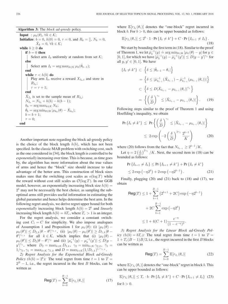
Since the proposed ad-greedy policy has bounded regret with-out considering the switching cost, it is easy to see that directlyapplying the ad-greedy policy can still result in bounded regreteven with switching cost. This holds because the best arm isguaranteed to be found in finite time, and thus, the total switch-ing cost will also be bounded. However, this does not mean thatthe ad-greedy policy will have the best performance when fac-ing switching cost. Typically, due to the additional penalty ofswitches, a good bandit algorithm needs to “explore in block”.This is done by grouping time slots and not switching duringthese slots. The proposed block ad-greedy policy that followsthis design philosophy is given in Algorithm 3. In order to focuson block exploration, here we present a version of the blockad-greedy policy for the baseline GGB. Later in Section IV-B,a version extended to handle multi-dimensional global param-eter is compared against the ad-greedy-2D policy. Thanks tothe block exploration structure, we show that the regret due toswitching cost is smaller for the block ad-greedy policy.


Another important note regarding the block ad-greedy policyis the choice of the block length h(b), which has not beenspecified. In the classic MAB problem with switching cost, suchas the one considered in [34], the block length is controlled to beexponentially increasing over time. This is because, as time goesby, the algorithm has more information about the true valuesof arms and hence the “block” size should increase to takeadvantage of the better arm. This construction of block sizesmakes sure that the switching cost scales as o(log T ) whilethe reward without cost still scales as O(log T ). In our GGBmodel, however, an exponentially increasing block size h(b) =2b may not be necessarily the best choice, as sampling the sub-optimal arms still provides useful information in estimating theglobal parameter and hence helps determine the best arm. In thefollowing regret analysis, we derive regret upper bound for bothexponentially increasing block length h(b) = 2b and linearlyincreasing block length h(b) = bTc , where Tc > 1 is an integer.

For the regret analysis, we consider a constant switch-ing cost Ct = C for simplicity. We also impose analoguesof Assumption 1 and Proposition 1 for μk (θ): (i) |μk (θ) −μk (θ′)| ≤ D2,k |θ − θ′|γ2 , k , (ii) |μk (θ) − μk (θ′)| ≥ D1,k |θ −θ′|γ1 , k for all k ∈ K, which implies that (i) |μk (θ) −μk (θ′)| ≤ D2 |θ − θ′|γ2 and (ii) |μ−1

k (y) − μ−1k (y′)| ≤ D|y −

y′|γ1 , where D2 = maxk∈K D2,k , γ2 = mink∈K γ2,k , γ1 =1/γ1 , γ1 = maxk∈K γ1,k and D = maxk∈K(1/D1,k )1/γ1 , k .

2) Regret Analysis for the Exponential Block ad-GreedyPolicy (h(b) = 2b ): The total regret from time t = 1 to T =2B − 1, i.e., the regret incurred in the first B blocks, can bewritten as

Reg(T ) =B−1∑b=0

E[rIb(θ∗)] (17)

where E[rIb(θ∗)] denotes the “one-block” regret incurred in

block b. For b > 0, this can be upper bounded as follows:

E[rIb(θ∗)] ≤ 2b · 1 · Pr {Ib �= k∗} + C · Pr {Ib+1 �= Ib} .

(18)We start by bounding the first term in (18). Similar to the proof

of Theorem 1, we let μ−1k (y) .= arg minθ∈Θ |μk (θ) − y| for y ∈

[0, 1], for which we have |μ−1k (y) − μ−1

k (y′)| ≤ D|y − y′|γ1 forall y, y′ ∈ [0, 1]. We have

{Ib �= k∗} ⊂{

δ ≤ |θb−1 − θ∗|}

={

δ ≤ |μ−1kb−1

(Xkb−1 ) − μ−1kb−1

(μkb−1 (θ∗))|}

⊂{

δ ≤ D|Xkb−1 − μkb−1 (θ∗)|γ1

}

={(

δ

D

)γ1

≤ |Xkb−1 − μkb−1 (θ∗)|}

. (19)

Following steps similar to the proof of Theorem 1 and usingHoeffding’s inequality, we obtain

Pr {Ib �= k∗} ≤ Pr

{(δ

D

)γ1

≤ |Xkb−1 − μkb−1 (θ∗)|}

≤ 2 exp

(−2(

δ

D

)2γ1 2b−1

K

)(20)

where (20) follows from the fact that Nkb−1 ≥ 2b−1/K.

Let η = 2(

δD

)2γ1/K. Next, the second item in (18) can be

bounded as follows:

Pr {Ib+1 �= Ib} ≤ Pr {Ib+1 �= k∗} + Pr {Ib �= k∗}≤ 2 exp

(−η2b)

+ 2 exp(−η2b−1) . (21)

Finally, plugging (20) and (21) back to (18) and (17), weobtain

Reg(T ) ≤ 1 +B−1∑b=1

(2b+1 + 2C

)exp(−η2b−1)

+ 2C

B−1∑b=1

exp(−η2b

)

≤ 1 + 4(C + 1)e−η

(1 − e−η )2 .

3) Regret Analysis for the Linear Block ad-Greedy Pol-icy (h(b) = bTc ): The total regret from time t = 1 to T =1 + Tc(B − 1)B/2, i.e., the regret incurred in the first B blockscan be written as

Reg(T ) =B−1∑b=0

E[rIb(θ∗)] (22)

where E[rIb(θ∗)] denotes the “one-block” regret in block b. This

can be upper bounded as follows:

E[rIb(θ∗)] ≤ Tc · b · Pr {Ib �= k∗} + C · Pr {Ib+1 �= Ib} (23)

for b > 0.


The first item in (23) can be further bounded as follows. First,we have

{Ib �= k∗} ⊂{

δ ≤ |θb−1 − θ∗|}

={

δ ≤ |μ−1kb−1

(Xkb−1 ) − μ−1kb−1

(μkb−1 (θ∗))|}

⊂{

δ ≤ D|Xkb−1 − μkb−1 (θ∗)|γ1

}

={(

δ

D

)γ1

≤ |Xkb−1 − μkb−1 (θ∗)|}

. (24)

Applying Hoeffding’s inequality, we obtain

Pr {Ib �= k∗} ≤ Pr

{(δ

D

)γ1

≤ |Xkb−1 − μkb−1 (θ∗)|}

≤ 2 exp

(−(

δ

D

)2γ1 (b − 1)2Tc

K

)(25)

where (25) follows from the fact that Nkb−1 ≥ (b − 1)2Tc/(2K).

Let κ = ( δD )2γ1 Tc

K . Next, the second term in (23) can bebounded as follows.

Pr {Ib+1 �= Ib} ≤ Pr {Ib+1 �= k∗} + Pr {Ib �= k∗}

≤ 2 exp(− κb2

)+ 2 exp

(− κ(b − 1)2

). (26)

Finally, plugging (25) and (26) back to (23) and (22), theregret is upper bounded as:

Reg(T ) ≤ 1 +B−1∑b=1

(2Tcb + 2C) exp(−κ(b − 1)2)

+ 2C

B−1∑b=1

exp(−κb2)

≤ 1 + 2Tc

B−2∑b=1

be−κb2+ (2Tc + 4C)

B−2∑b=0

e−κb2

≤ 1 + 2Tce−

12√

2κ+ 2Tc

∫ B−2

0ze−κz 2

dz

+ (2Tc + 4C)B−2∑b=0

e−κb

≤ 1 + 2Tce−

12√

2κ+ Tc

1κ

+ (2Tc + 4C)1

eκ − 1.

Although both linear and exponential block size can achievea bounded regret for block ad-greedy with switching cost, theanalysis here only reflects the upper bounds of the regret, notnecessarily the actual performance. We will evaluate their per-formances in the coverage optimization problems and report thesimulation results in Section IV-B.

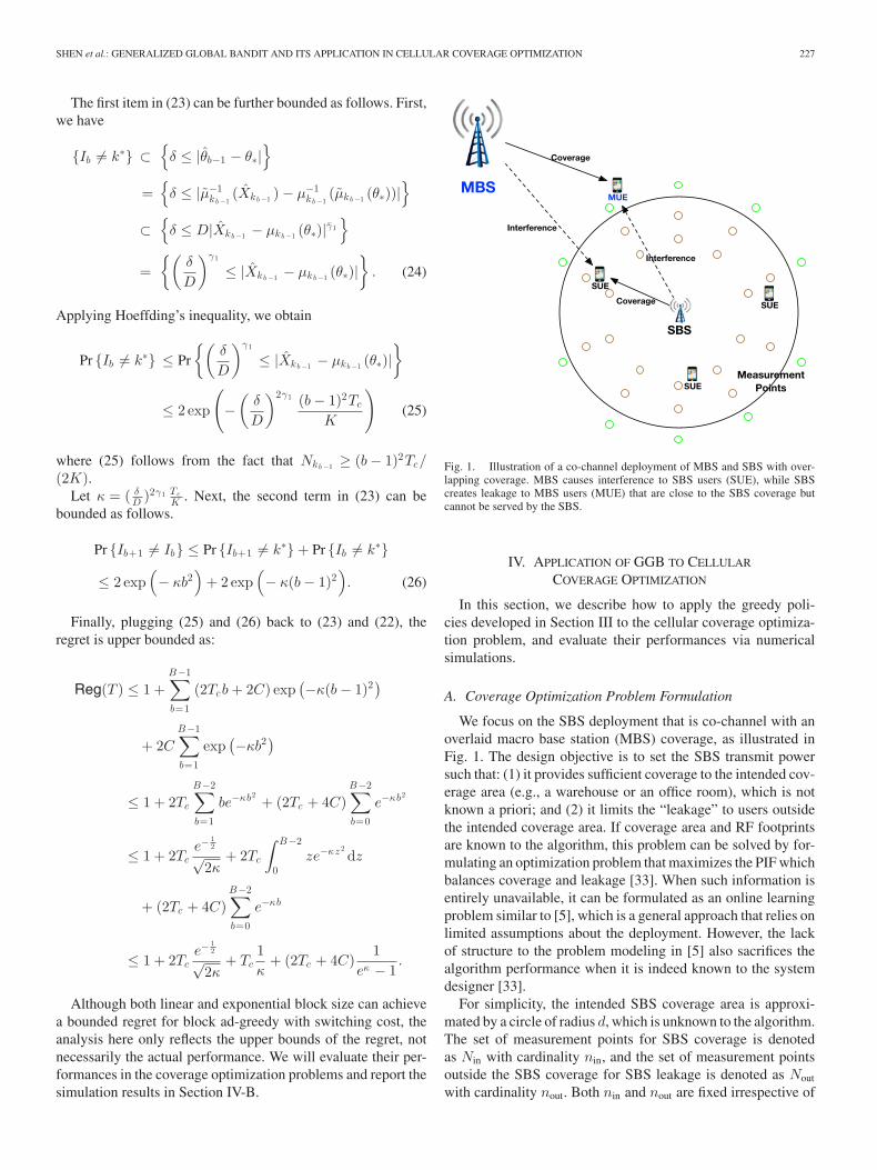
Fig. 1. Illustration of a co-channel deployment of MBS and SBS with over-lapping coverage. MBS causes interference to SBS users (SUE), while SBScreates leakage to MBS users (MUE) that are close to the SBS coverage butcannot be served by the SBS.

IV. APPLICATION OF GGB TO CELLULAR

COVERAGE OPTIMIZATION

In this section, we describe how to apply the greedy poli-cies developed in Section III to the cellular coverage optimiza-tion problem, and evaluate their performances via numericalsimulations.

A. Coverage Optimization Problem Formulation

We focus on the SBS deployment that is co-channel with anoverlaid macro base station (MBS) coverage, as illustrated inFig. 1. The design objective is to set the SBS transmit powersuch that: (1) it provides sufficient coverage to the intended cov-erage area (e.g., a warehouse or an office room), which is notknown a priori; and (2) it limits the “leakage” to users outsidethe intended coverage area. If coverage area and RF footprintsare known to the algorithm, this problem can be solved by for-mulating an optimization problem that maximizes the PIF whichbalances coverage and leakage [33]. When such information isentirely unavailable, it can be formulated as an online learningproblem similar to [5], which is a general approach that relies onlimited assumptions about the deployment. However, the lackof structure to the problem modeling in [5] also sacrifices thealgorithm performance when it is indeed known to the systemdesigner [33].

For simplicity, the intended SBS coverage area is approxi-mated by a circle of radius d, which is unknown to the algorithm.The set of measurement points for SBS coverage is denotedas Nin with cardinality nin, and the set of measurement pointsoutside the SBS coverage for SBS leakage is denoted as Nout

with cardinality nout. Both nin and nout are fixed irrespective of


the deployment. Furthermore, we assume that the measurementpoints have uniformly distributed distances to the SBS, forboth inside and outside routes. Such uniform spacing has beensimilarly adopted in [35] for evaluation of the area spectralefficiency. In practice, choosing the measurement points forcoverage estimation and optimization has been studied in [33],which has argued that uniform sampling of the area offers theleast bias to the algorithm. Practical methods to collect suchmeasurement reports without repeated measurements havealso been proposed in [33]. Furthermore, we note that thisassumption on measurement point placement is not crucial toour algorithm because it only affects the specific format of theobjective function. In other words, other reasonable setup forthe measurement points can be adopted and it will only resultin a change of the objective function as described in (27).

We consider maximizing the total spectral efficiency of themeasurement points under a proportional fairness constraint.This has been proved to be equivalent to maximizing the sumof logarithms of the user rate [36]. Formally, we have

fk (d, Pm ) = α∑i∈N in

g(RSBS,i (d, Pm ))

+ (1 − α)∑

i∈Nout

g(RMBS,i (d, Pm )), (27)

where d denotes the radius of the intended coverage area, Pm

denotes the average MBS received signal power, RSBS (d, Pm )and RMBS (d, Pm ) denote the rate function for SBS-served andMBS-served users, respectively, and α is a weight coefficientthat balances coverage and leakage. A large α suggests that thedesign favors having sufficient SBS coverage over leakage thataffects MBS users, and vice versa. Subscript k indicates that SBSadopts transmit power Pk ∈ {P1 , . . . , PK : P1 < · · · < PK }.We note that the reward function (27) is defined for each indi-vidual SBS if a distributed deployment is considered, in which(27) can be different across SBSs.

For evaluation of the proposed solutions, in the following wefocus on some specific system configurations. Since we haveassumed a uniform placement of measurement points for Nin

and Nout, we can re-write (27) as

fk (d, Pm ) = α

n in∑i=1

log(

RSBS

(i

nind, Pm

))

+ (1 − α)nout∑i=1

log(

RMBS

((1 +

i

nin

)d, Pm

))

.= αf(1)k (d, Pm ) + (1 − α)f (2)

k (d, Pm ). (28)

Denoting the pathloss function as PL(d), the received signalpower at distance d1 from the SBS with transmit power Pk canbe written as

Pr (d1)[dB] = Pk [dB] − PL(d1)[dB] + δ, (29)

where δ denotes the shadowing fading in the dB domain. Notethat PL(d) can be any reasonable pathloss model that fits the

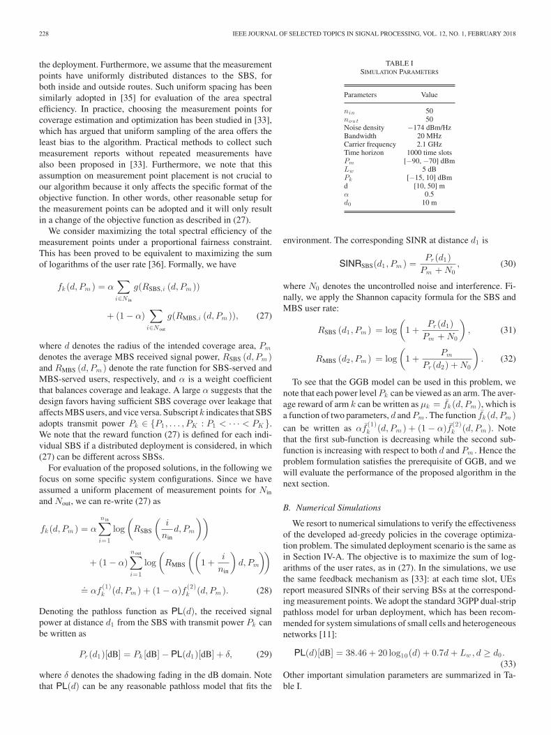
TABLE ISIMULATION PARAMETERS

Parameters Value

nin 50nou t 50Noise density −174 dBm/HzBandwidth 20 MHzCarrier frequency 2.1 GHzTime horizon 1000 time slotsPm [−90, −70] dBmLw 5 dBPk [−15, 10] dBmd [10, 50] mα 0.5d0 10 m

environment. The corresponding SINR at distance d1 is

SINRSBS(d1 , Pm ) =Pr (d1)

Pm + N0, (30)

where N0 denotes the uncontrolled noise and interference. Fi-nally, we apply the Shannon capacity formula for the SBS andMBS user rate:

RSBS (d1 , Pm ) = log(

1 +Pr (d1)

Pm + N0

), (31)

RMBS (d2 , Pm ) = log(

1 +Pm

Pr (d2) + N0

). (32)

To see that the GGB model can be used in this problem, wenote that each power level Pk can be viewed as an arm. The aver-age reward of arm k can be written as μk = fk (d, Pm ), which isa function of two parameters, d and Pm . The function fk (d, Pm )can be written as αf

(1)k (d, Pm ) + (1 − α)f (2)

k (d, Pm ). Notethat the first sub-function is decreasing while the second sub-function is increasing with respect to both d and Pm . Hence theproblem formulation satisfies the prerequisite of GGB, and wewill evaluate the performance of the proposed algorithm in thenext section.

B. Numerical Simulations

We resort to numerical simulations to verify the effectivenessof the developed ad-greedy policies in the coverage optimiza-tion problem. The simulated deployment scenario is the same asin Section IV-A. The objective is to maximize the sum of log-arithms of the user rates, as in (27). In the simulations, we usethe same feedback mechanism as [33]: at each time slot, UEsreport measured SINRs of their serving BSs at the correspond-ing measurement points. We adopt the standard 3GPP dual-strippathloss model for urban deployment, which has been recom-mended for system simulations of small cells and heterogeneousnetworks [11]:

PL(d)[dB] = 38.46 + 20 log10(d) + 0.7d + Lw , d ≥ d0 .(33)

Other important simulation parameters are summarized in Ta-ble I.


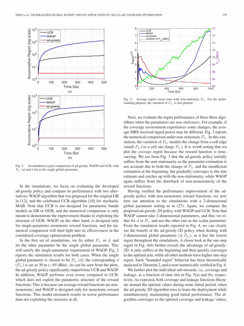
Fig. 2. Accumulative regret comparison of ad-greedy, WAGP and UCB, withPm (a) and d (b) as the single global parameter.

In the simulations, we focus on evaluating the developedad-greedy policy and compare its performance with two alter-natives: WAGP algorithm that was proposed for the original GBin [12], and the celebrated UCB algorithm [10] for stochasticMAB. Note that UCB is not designed for parametric banditmodels as GB or GGB, and the numerical comparison is onlymeant to demonstrate the improvement thanks to exploiting thestructure of GGB. WAGP, on the other hand, is designed onlyfor single-parameter monotonic reward functions, and the nu-merical comparison will shed light into its effectiveness in theconsidered coverage optimization problem.

In the first set of simulations, we fix either Pm or d, andlet the other parameter be the single global parameter. Thiswill satisfy the single-parameter requirement of WAGP. Fig. 2reports the simulation results for both cases. When the singleglobal parameter is chosen to be Pm (d), the corresponding d(Pm ) is set as 30 m (−85 dBm). As can be seen from the plots,the ad-greedy policy significantly outperforms UCB and WAGP.In addition, WAGP performs even worse compared to UCB,which does not exploit the parametric structure of the rewardfunctions. This is because our average reward functions are non-monotonic, and WAGP is designed only for monotonic rewardfunctions. This model mismatch results in worse performancethan not exploiting the structure at all.

Fig. 3. Average regret versus time with non-stationary Pm . For the under-standing purpose, the variation of Pm is also plotted.

Next, we evaluate the regret performance of these three algo-rithms when the parameters are non-stationary. For example, ifthe coverage environment experiences some changes, the aver-age MBS received signal power may be different. Fig. 3 reportsthe numerical comparison under non-stationary Pm . In this sim-ulation, the variation of Pm models the change from a cell edge(small Pm ) to a cell site (large Pm ). It is worth noting that weplot the average regret because the reward function is time-varying. We see from Fig. 3 that the ad-greedy policy initiallysuffers from the non-stationarity as the parameter estimation isnot accurate due to both the change of Pm and the insufficientestimation at the beginning, but gradually converges to the trueestimate and catches up with the non-stationarity, while WAGPagain suffers from the drawback of non-monotonicity of thereward functions.

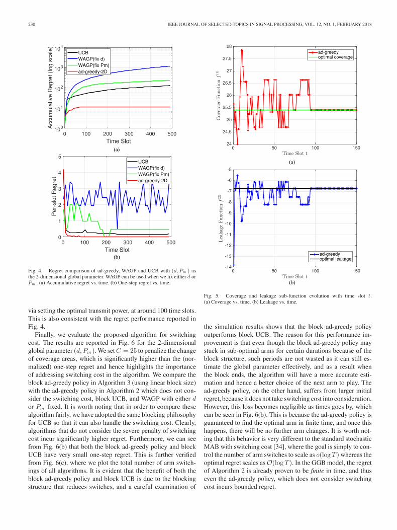
Having verified the performance improvement of the ad-greedy policy with non-monotonic reward functions, we nowturn our attention to the simulations with a 2-dimensionalglobal parameter setting as in (27). Again, we compare theproposed ad-greedy-2D policy with WAGP and UCB. Note thatWAGP cannot take 2-dimensional parameters, and thus we ei-ther fix d or Pm and use the other one as the scalar parameter.From the simulation results reported in Fig. 4, we can clearlysee the benefit of the ad-greedy-2D policy when dealing with2-dimensional global parameter (d, Pm ), as it has the lowestregret throughout the simulations. A closer look at the one-stepregret in Fig. 4(b) further reveals the advantage of ad-greedy-2D: it only suffers at the beginning and then quickly convergesto the optimal arm, while all other methods have higher one-stepregret. Such “bounded regret” behavior has been theoreticallyanalyzed in Theorem 2, and is now numerically verified in Fig. 4.

We further plot the individual sub-rewards, i.e., coverage andleakage, as a function of time slot in Fig. 5(a) and (b), respec-tively. As expected, both coverage and leakage functions fluctu-ate around the optimal values during some initial period, whenthe ad-greedy-2D algorithm tries to learn the deployment whilesimultaneously maintaining good initial performance. The al-gorithm converges to the optimal coverage and leakage values,


Fig. 4. Regret comparison of ad-greedy, WAGP and UCB with (d, Pm ) asthe 2-dimensional global parameter. WAGP can be used when we fix either d orPm . (a) Accumulative regret vs. time. (b) One-step regret vs. time.

via setting the optimal transmit power, at around 100 time slots.This is also consistent with the regret performance reported inFig. 4.

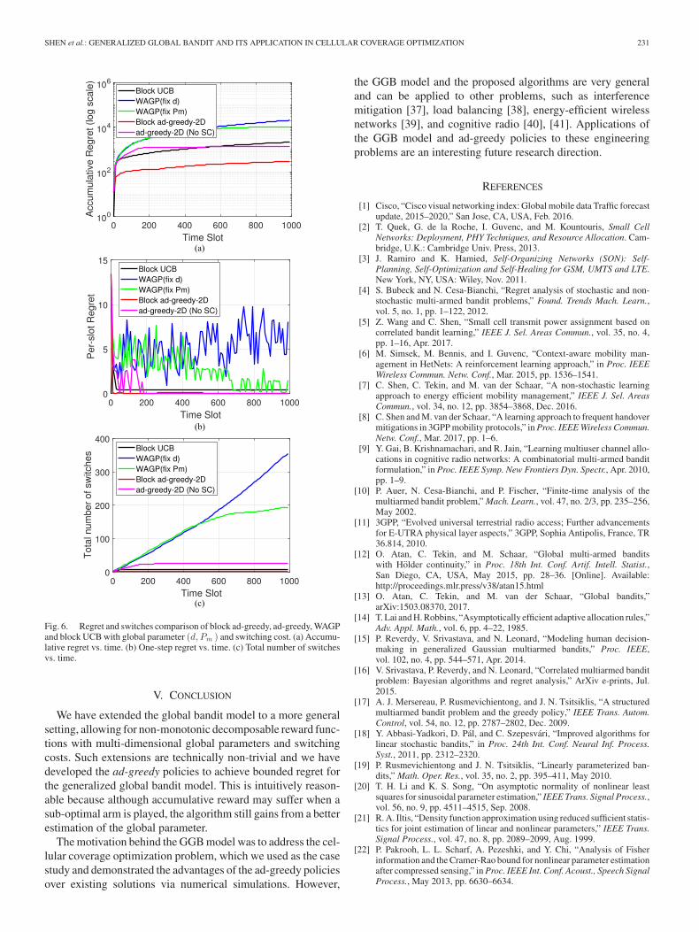
Finally, we evaluate the proposed algorithm for switchingcost. The results are reported in Fig. 6 for the 2-dimensionalglobal parameter (d, Pm ). We set C = 25 to penalize the changeof coverage areas, which is significantly higher than the (nor-malized) one-step regret and hence highlights the importanceof addressing switching cost in the algorithm. We compare theblock ad-greedy policy in Algorithm 3 (using linear block size)with the ad-greedy policy in Algorithm 2 which does not con-sider the switching cost, block UCB, and WAGP with either dor Pm fixed. It is worth noting that in order to compare thesealgorithm fairly, we have adopted the same blocking philosophyfor UCB so that it can also handle the switching cost. Clearly,algorithms that do not consider the severe penalty of switchingcost incur significantly higher regret. Furthermore, we can seefrom Fig. 6(b) that both the block ad-greedy policy and blockUCB have very small one-step regret. This is further verifiedfrom Fig. 6(c), where we plot the total number of arm switch-ings of all algorithms. It is evident that the benefit of both theblock ad-greedy policy and block UCB is due to the blockingstructure that reduces switches, and a careful examination of

Fig. 5. Coverage and leakage sub-function evolution with time slot t.(a) Coverage vs. time. (b) Leakage vs. time.

the simulation results shows that the block ad-greedy policyoutperforms block UCB. The reason for this performance im-provement is that even though the block ad-greedy policy maystuck in sub-optimal arms for certain durations because of theblock structure, such periods are not wasted as it can still es-timate the global parameter effectively, and as a result whenthe block ends, the algorithm will have a more accurate esti-mation and hence a better choice of the next arm to play. Thead-greedy policy, on the other hand, suffers from larger initialregret, because it does not take switching cost into consideration.However, this loss becomes negligible as times goes by, whichcan be seen in Fig. 6(b). This is because the ad-greedy policy isguaranteed to find the optimal arm in finite time, and once thishappens, there will be no further arm changes. It is worth not-ing that this behavior is very different to the standard stochasticMAB with switching cost [34], where the goal is simply to con-trol the number of arm switches to scale as o(log T ) whereas theoptimal regret scales as O(log T ). In the GGB model, the regretof Algorithm 2 is already proven to be finite in time, and thuseven the ad-greedy policy, which does not consider switchingcost incurs bounded regret.


Fig. 6. Regret and switches comparison of block ad-greedy, ad-greedy, WAGPand block UCB with global parameter (d, Pm ) and switching cost. (a) Accumu-lative regret vs. time. (b) One-step regret vs. time. (c) Total number of switchesvs. time.

V. CONCLUSION

We have extended the global bandit model to a more generalsetting, allowing for non-monotonic decomposable reward func-tions with multi-dimensional global parameters and switchingcosts. Such extensions are technically non-trivial and we havedeveloped the ad-greedy policies to achieve bounded regret forthe generalized global bandit model. This is intuitively reason-able because although accumulative reward may suffer when asub-optimal arm is played, the algorithm still gains from a betterestimation of the global parameter.

The motivation behind the GGB model was to address the cel-lular coverage optimization problem, which we used as the casestudy and demonstrated the advantages of the ad-greedy policiesover existing solutions via numerical simulations. However,

the GGB model and the proposed algorithms are very generaland can be applied to other problems, such as interferencemitigation [37], load balancing [38], energy-efficient wirelessnetworks [39], and cognitive radio [40], [41]. Applications ofthe GGB model and ad-greedy policies to these engineeringproblems are an interesting future research direction.

REFERENCES

[1] Cisco, “Cisco visual networking index: Global mobile data Traffic forecastupdate, 2015–2020,” San Jose, CA, USA, Feb. 2016.

[2] T. Quek, G. de la Roche, I. Guvenc, and M. Kountouris, Small CellNetworks: Deployment, PHY Techniques, and Resource Allocation. Cam-bridge, U.K.: Cambridge Univ. Press, 2013.

[3] J. Ramiro and K. Hamied, Self-Organizing Networks (SON): Self-Planning, Self-Optimization and Self-Healing for GSM, UMTS and LTE.New York, NY, USA: Wiley, Nov. 2011.

[4] S. Bubeck and N. Cesa-Bianchi, “Regret analysis of stochastic and non-stochastic multi-armed bandit problems,” Found. Trends Mach. Learn.,vol. 5, no. 1, pp. 1–122, 2012.

[5] Z. Wang and C. Shen, “Small cell transmit power assignment based oncorrelated bandit learning,” IEEE J. Sel. Areas Commun., vol. 35, no. 4,pp. 1–16, Apr. 2017.

[6] M. Simsek, M. Bennis, and I. Guvenc, “Context-aware mobility man-agement in HetNets: A reinforcement learning approach,” in Proc. IEEEWireless Commun. Netw. Conf., Mar. 2015, pp. 1536–1541.

[7] C. Shen, C. Tekin, and M. van der Schaar, “A non-stochastic learningapproach to energy efficient mobility management,” IEEE J. Sel. AreasCommun., vol. 34, no. 12, pp. 3854–3868, Dec. 2016.

[8] C. Shen and M. van der Schaar, “A learning approach to frequent handovermitigations in 3GPP mobility protocols,” in Proc. IEEE Wireless Commun.Netw. Conf., Mar. 2017, pp. 1–6.

[9] Y. Gai, B. Krishnamachari, and R. Jain, “Learning multiuser channel allo-cations in cognitive radio networks: A combinatorial multi-armed banditformulation,” in Proc. IEEE Symp. New Frontiers Dyn. Spectr., Apr. 2010,pp. 1–9.

[10] P. Auer, N. Cesa-Bianchi, and P. Fischer, “Finite-time analysis of themultiarmed bandit problem,” Mach. Learn., vol. 47, no. 2/3, pp. 235–256,May 2002.

[11] 3GPP, “Evolved universal terrestrial radio access; Further advancementsfor E-UTRA physical layer aspects,” 3GPP, Sophia Antipolis, France, TR36.814, 2010.

[12] O. Atan, C. Tekin, and M. Schaar, “Global multi-armed banditswith Holder continuity,” in Proc. 18th Int. Conf. Artif. Intell. Statist.,San Diego, CA, USA, May 2015, pp. 28–36. [Online]. Available:http://proceedings.mlr.press/v38/atan15.html

[13] O. Atan, C. Tekin, and M. van der Schaar, “Global bandits,”arXiv:1503.08370, 2017.

[14] T. Lai and H. Robbins, “Asymptotically efficient adaptive allocation rules,”Adv. Appl. Math., vol. 6, pp. 4–22, 1985.

[15] P. Reverdy, V. Srivastava, and N. Leonard, “Modeling human decision-making in generalized Gaussian multiarmed bandits,” Proc. IEEE,vol. 102, no. 4, pp. 544–571, Apr. 2014.

[16] V. Srivastava, P. Reverdy, and N. Leonard, “Correlated multiarmed banditproblem: Bayesian algorithms and regret analysis,” ArXiv e-prints, Jul.2015.

[17] A. J. Mersereau, P. Rusmevichientong, and J. N. Tsitsiklis, “A structuredmultiarmed bandit problem and the greedy policy,” IEEE Trans. Autom.Control, vol. 54, no. 12, pp. 2787–2802, Dec. 2009.

[18] Y. Abbasi-Yadkori, D. Pal, and C. Szepesvari, “Improved algorithms forlinear stochastic bandits,” in Proc. 24th Int. Conf. Neural Inf. Process.Syst., 2011, pp. 2312–2320.

[19] P. Rusmevichientong and J. N. Tsitsiklis, “Linearly parameterized ban-dits,” Math. Oper. Res., vol. 35, no. 2, pp. 395–411, May 2010.

[20] T. H. Li and K. S. Song, “On asymptotic normality of nonlinear leastsquares for sinusoidal parameter estimation,” IEEE Trans. Signal Process.,vol. 56, no. 9, pp. 4511–4515, Sep. 2008.

[21] R. A. Iltis, “Density function approximation using reduced sufficient statis-tics for joint estimation of linear and nonlinear parameters,” IEEE Trans.Signal Process., vol. 47, no. 8, pp. 2089–2099, Aug. 1999.

[22] P. Pakrooh, L. L. Scharf, A. Pezeshki, and Y. Chi, “Analysis of Fisherinformation and the Cramer-Rao bound for nonlinear parameter estimationafter compressed sensing,” in Proc. IEEE Int. Conf. Acoust., Speech SignalProcess., May 2013, pp. 6630–6634.


[23] 3GPP, “Evolved universal terrestrial radio access; Self-configuring andself-optimizing network (SON) use cases and solutions,” 3GPP, SophiaAntipolis, France, TR 36.902, 2010.

[24] Cisco, San Jose, CA, USA, Cisco SON for Small Cells, White Paper,2015.

[25] Qualcomm Research, San Diego, CA, USA, Cost-effective EnterpriseSmall Cell Deployment with UltraSON, Apr. 2016, White Paper.

[26] G. Hampel, K. L. Clarkson, J. D. Hobby, and P. A. Polakos, “The tradeoffbetween coverage and capacity in dynamic optimization of 3G cellularnetworks,” in Proc. IEEE 58th Veh. Technol. Conf., Oct. 2003, vol. 2,pp. 927–932.

[27] A. Engels, M. Reyer, X. Xu, R. Mathar, J. Zhang, and H. Zhuang, “Au-tonomous self-optimization of coverage and capacity in LTE cellular net-works,” IEEE Trans. Veh. Technol., vol. 62, no. 5, pp. 1989–2004, Jun.2013.

[28] O. N. C. Yilmaz, S. Hamalainen, and J. Hamalainen, “Analysis of antennaparameter optimization space for 3GPP LTE,” in Proc. IEEE 70th Veh.Technol.—Fall, Sep. 2009, pp. 1–5.

[29] S. Jin, J. Wang, Q. Sun, M. Matthaiou, and X. Gao, “Cell coverage op-timization for the multicell Massive MIMO uplink,” IEEE Trans. Veh.Technol., vol. 64, no. 12, pp. 5713–5727, Dec. 2015.

[30] S. Berger, M. Simsek, A. Fehske, P. Zanier, I. Viering, and G. Fettweis,“Joint downlink and uplink tilt-based self-organization of coverage andcapacity under sparse system knowledge,” IEEE Trans. Veh. Technol.,vol. 65, no. 4, pp. 2259–2273, Apr. 2016.

[31] H. Claussen, L. T. W. Ho, and L. G. Samuel, “Self-optimization of cov-erage for femtocell deployments,” in Proc. Wireless Telecommun. Symp.,Apr. 2008, pp. 278–285.

[32] S. Nagaraja et al., “Transmit power self-calibration for residentialUMTS/HSPA+ femtocells,” in Proc. Int. Symp. Modeling Optim. Mobile,Ad Hoc, and Wireless Netw., May 2011, pp. 451–455.

[33] S. Nagaraja et al., “Downlink transmit power calibration for enterprisefemtocells,” in Proc. IEEE Veh. Technol. Conf., 2011, pp. 1–5.

[34] R. Agrawal, M. V. Hegde, and D. Teneketzis, “Asymptotically efficientadaptive allocation rules for the multiarmed bandit problem with switchingcost,” IEEE Trans. Autom. Control, vol. 33, no. 10, pp. 899–906, Oct. 1988.

[35] M. S. Alouini and A. Goldsmith, “Area spectral efficiency of cellularmobile radio systems,” in Proc. IEEE Veh. Technol. Conf., May 1997,vol. 2, pp. 652–656.

[36] J.-Y. Le Boudec, “Rate adaptation, congestion control and fair-ness: A tutorial,” 2005, unpublished manuscript. [Online]. Available:http://ica1www.epfl.ch/PS_files/LEB3132.pdf

[37] M. Bennis, S. Perlaza, P. Blasco, Z. Han, and H. Poor, “Self-organizationin small cell networks: A reinforcement learning approach,” IEEE Trans.Wireless Commun., vol. 12, no. 7, pp. 3202–3212, Jul. 2013.

[38] I. Koutsopoulos and L. Tassiulas, “Joint optimal access point selectionand channel assignment in wireless networks,” IEEE/ACM Trans. Netw.,vol. 15, no. 3, pp. 521–532, Jun. 2007.

[39] N. Mastronarde and M. van der Schaar, “Fast reinforcement learning forenergy-efficient wireless communication,” IEEE Trans. Signal Process.,vol. 59, no. 12, pp. 6262–6266, Dec. 2011.

[40] H. P. Shiang and M. van der Schaar, “Delay-sensitive resource manage-ment in multi-hop cognitive radio networks,” in Proc. 3rd IEEE Symp.New Frontiers Dyn. Spectr. Access Netw., Oct. 2008, pp. 1–12.

[41] M. S. Greco, F. Gini, and P. Stinco, “Cognitive radars: Some appli-cations,” in Proc. IEEE Global Conf. Signal Inf. Process., Dec. 2016,pp. 1077–1082.

Cong Shen (S’01–M’09–SM’15) received the B.S.and M.S. degrees from the Department of ElectronicEngineering, Tsinghua University, Beijing, China.,in 2002 and 2004, respectively He received the Ph.D.degree from the Electrical Engineering Department,UCLA, Los Angeles, CA, USA, in 2009. From2009 to 2014, he was with Qualcomm Research,San Diego, CA, USA, where he focused on vari-ous cutting-edge research topics including cognitiveradio, TV white space, heterogeneous and ultradensenetworks. In 2015, he returned to academia and joined

the School of Information Science and Technology, University of Science andTechnology of China (USTC) as the 100 Talents Program Professor. His gen-eral research interests include communication theory, wireless networks, andmachine learning. Currently, he serves as an editor for the IEEE TRANSACTIONS

ON WIRELESS COMMUNICATIONS.

Ruida Zhou is currently a Senior UndergraduateStudent at the School of Information Science andTechnology, University of Science and Technologyof China (USTC), Hefei, China. His research inter-ests include machine learning, information theory,and statistics.

Cem Tekin (M’13) received the B.Sc. degree in elec-trical and electronics engineering from the MiddleEast Technical University, Ankara, Turkey, in 2008,the M.S.E. degree in electrical engineering: systems,the M.S. degree in mathematics, and the Ph.D. degreein electrical engineering: systems from the Universityof Michigan, Ann Arbor, MI, USA, in 2010, 2011,and 2013, respectively. He is an Assistant Professorwith the Electrical and Electronics Engineering De-partment, Bilkent University, Ankara, Turkey. FromFebruary 2013 to January 2015, he was a Postdoctoral

Scholar with the University of California, Los Angeles. His research interestsinclude machine learning, multiarmed bandit problems, data mining, multiagentsystems, and smart healthcare. He received the University of Michigan Elec-trical Engineering Departmental Fellowship in 2008, and the Fred W. EllersickAward for the best paper in MILCOM 2009.

Mihaela van der Schaar (F’09) is currently a ManProfessor of quantitative finance with the Oxford–Man Institute of Quantitative Finance (OMI),Oxford, U.K. and the Department of Engineering Sci-ence, University of Oxford, Oxford, U.K., a Fellowof Christ Church College, and a Faculty Fellow ofthe Alan Turing Institute, London, UK. She is also aChancellor’s Professor of electrical engineering withthe University of California, Los Angeles, CA, USA.Her current research interests include machine learn-ing, data science and decisions for medicine, educa-

tion, and finance. She was a Distinguished Lecturer of the CommunicationsSociety, the Editor-in-Chief of the IEEE TRANSACTIONS ON MULTIMEDIA, aSenior Editorial Board member of the Editorial Board of the IEEE JOURNAL ON

SELECTED TOPICS IN SIGNAL PROCESSING (JSTSP) and the IEEE JOURNAL ON

EMERGING AND SELECTED TOPICS IN CIRCUITS AND SYSTEMS (JETCAS). Shereceived an NSF CAREER Award (2004), the Best Paper Award from IEEETRANSACTIONS ON CIRCUITS AND SYSTEMS for Video Technology (2005), theOkawa Foundation Award (2006), the IBM Faculty Award (2005, 2007, 2008),the Most Cited Paper Award from the EURASIP: Image Communications Jour-nal (2006), the Gamenets Conference Best Paper Award (2011), and the 2011IEEE Circuits and Systems Society Darlington Award Best Paper Award. Sheplayed a lead role in the MPEG video compression and streaming internationalstandardization activities for which she received 3 ISO Awards and for whichshe holds 33 granted US patents.

Documents

Generalized Global Bandit and Its Application in Cellular