General Constructions

General Constructions

Constructing Optimal Phylogenetic Networks in

General

Optimal = minimum number of recombinations. Called Min ARG.

The method is based on the coalescent

viewpoint of sequence evolution. We build

the network backwards in time.

A Heuristic for Constructing a good ARG

• The method is an adaptation of the ``history” lower bound (Myers).

• A non-informative column is one with fewer than two 0’s or fewer than two 1’s.

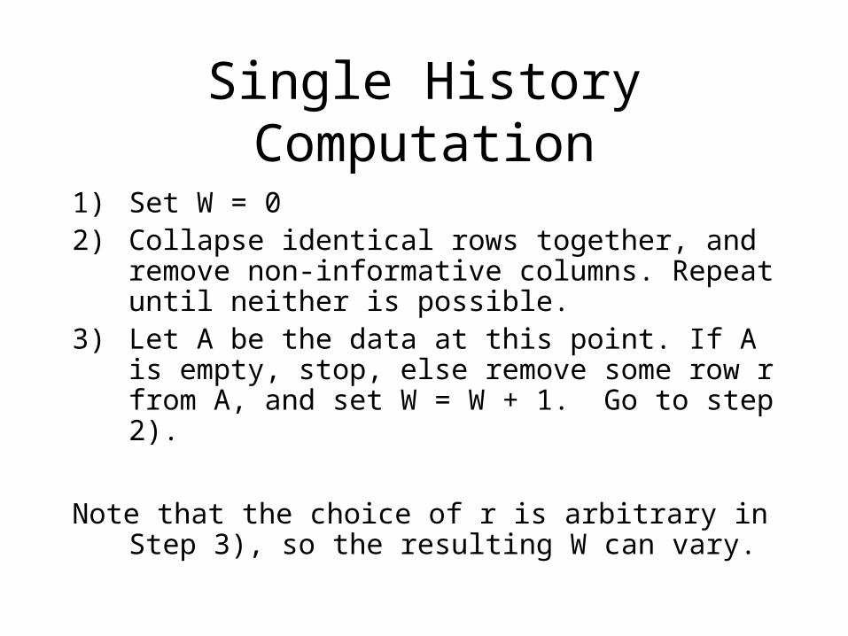
Single History Computation

1) Set W = 02) Collapse identical rows together, and remove non-

informative columns. Repeat until neither is possible.

3) Let A be the data at this point. If A is empty, stop, else remove some row r from A, and set W = W + 1. Go to step 2).

Note that the choice of r is arbitrary in Step 3), so the resulting W can vary.

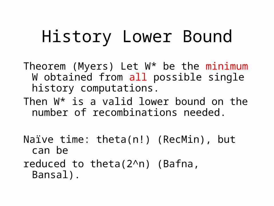
History Lower Bound

Theorem (Myers) Let W* be the minimum W obtained from all possible single history computations.

Then W* is a valid lower bound on the number of recombinations needed.

Naïve time: theta(n!) (RecMin), but can bereduced to theta(2^n) (Bafna, Bansal).

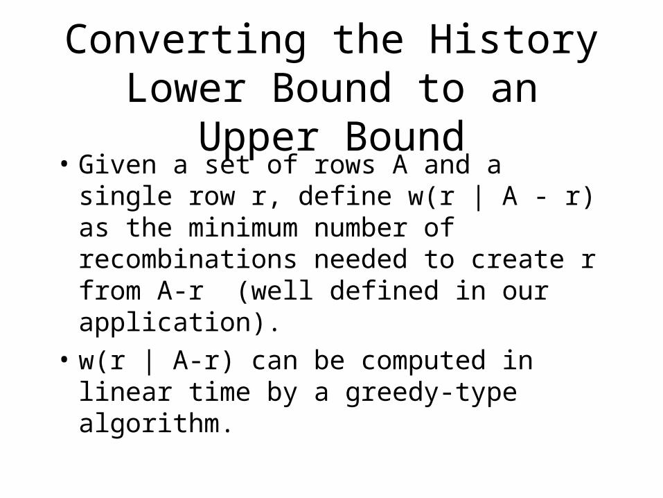
Converting the History Lower Bound to an Upper Bound

• Given a set of rows A and a single row r, define w(r | A - r) as the minimum number of recombinations needed to create r from A-r (well defined in our application).

• w(r | A-r) can be computed in linear time by a greedy-type algorithm.

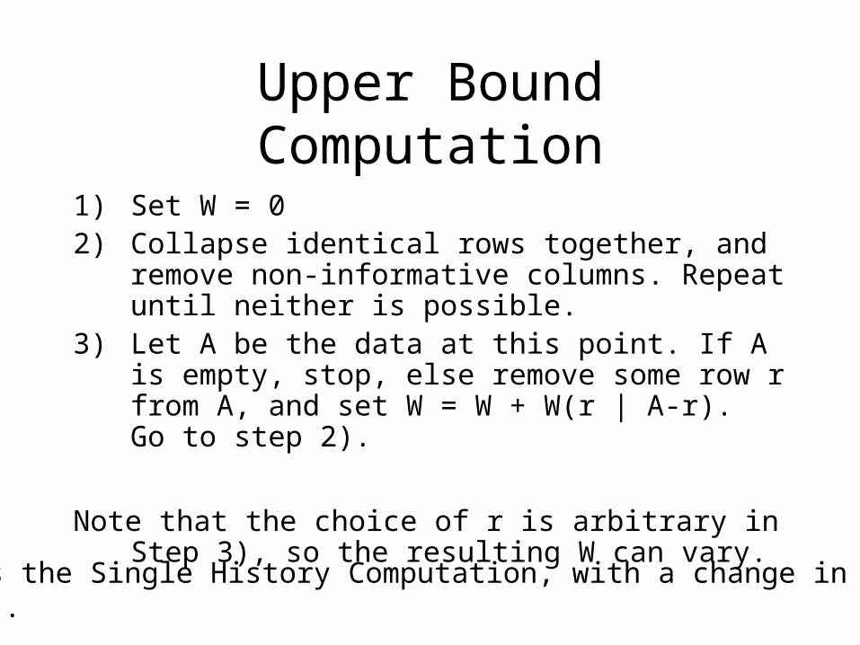
Upper Bound Computation

1) Set W = 02) Collapse identical rows together, and remove non-

informative columns. Repeat until neither is possible.

3) Let A be the data at this point. If A is empty, stop, else remove some row r from A, and set W = W + W(r | A-r). Go to step 2).

Note that the choice of r is arbitrary in Step 3), so the resulting W can vary.

This is the Single History Computation, with a change instep 3).

Note, even a single execution of the upper bound computation gives a valid upper bound, and a way to construct a network. This is in contrast to the History Bound which requires finding the minimum W over all histories.

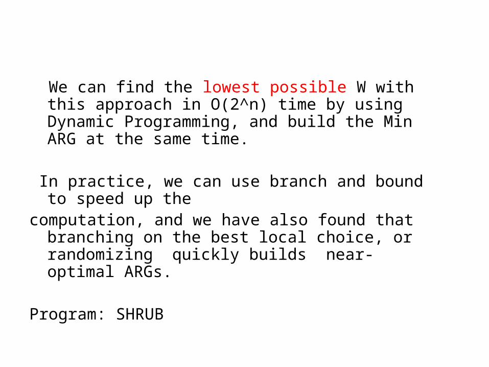
We can find the lowest possible W with this approach in O(2^n) time by using Dynamic Programming, and build the Min ARG at the same time.

In practice, we can use branch and bound to speed up the

computation, and we have also found that branching on the best local choice, or randomizing quickly builds near-optimal ARGs.

Program: SHRUB

Branch and Bound

(Branching) In Step 3) choose r to minimize w(r | A-r) + L(A-r), where L(A-r) is some fast

lower bound on the number of recombinations needed for the set A-r. Even HK is good for this purpose.

(Bounding) Let C be the min for an full solution found so far; If W + L(A) >= C, then backtrack.

Kreitman’s 1983 ADH Data

• 11 sequences, 43 segregating sites

• Both HapBound and SHRUB took only a fraction of a second to analyze this data.

• Both produced 7 for the number of detected recombination events

Therefore, independently of all other methods, our lower and upper bound methods together imply that 7 is the minimum number of recombination events.

A minimal ARG for Kreitman’s data

QuickTime™ and aTIFF (LZW) decompressor

are needed to see this picture.

SHRUB produces code that can be input to an open source program to display the constructed ARG

The Human LPL Data (Nickerson et al. 1998)





Our new lower and upper bounds

Optimal RecMin Bounds

(We ignored insertion/deletion, unphased sites, and sites with missing data.)

(88 Sequences, 88 sites)

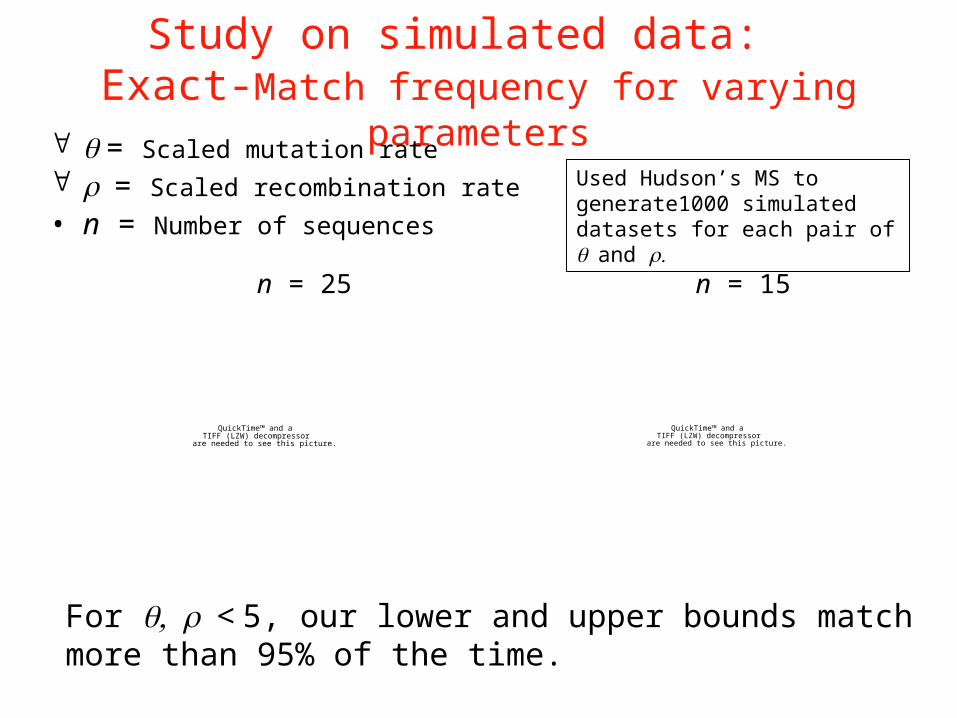
Study on simulated data: Exact-Match frequency for varying parameters

= Scaled mutation rate = Scaled recombination rate

• n = Number of sequences



n = 25

For < 5, our lower and upper bounds match more than 95% of the time.

Used Hudson’s MS to generate1000 simulated datasets for each pair of and



n = 15

Exact-Match frequency for varying number of sequences

Match frequency does not depend on n as much as it does on or



A closer look at the deviation

Average ratio of lower bound to upper bound when they do not match



For n = 25:

The numerical difference between lower and upper bounds grows as or increases, but their ratio is more stable.

Part III: Applications

Uniform Sampling of Min ARGs

• Sampling of ARGs: useful in statistical applications, but thought to be very challenging computationally. How to sample uniformly over the set of Min ARGs?

• All-visible ARGs: A special type of ARG – Built with only the input sequences– An all-visible ARG is a Min ARG

• We have an O(2n) algorithm to sample uniformly from the all-visible ARGs.– Practical when the number of sites is small

• We have heuristics to sample Min ARGs when there is no all-visible ARG.

Application: Association Mapping

• Given case-control data M, uniformly sample the minimum ARGs (in practice for small windows of fixed number of SNPs)

• Build the ``marginal” tree for each interval between adjacent recombination points in the ARG

• Look for non-random clustering of cases in the tree; accumulate statistics over the trees to find the best mutation explaining the partition into cases and controls.

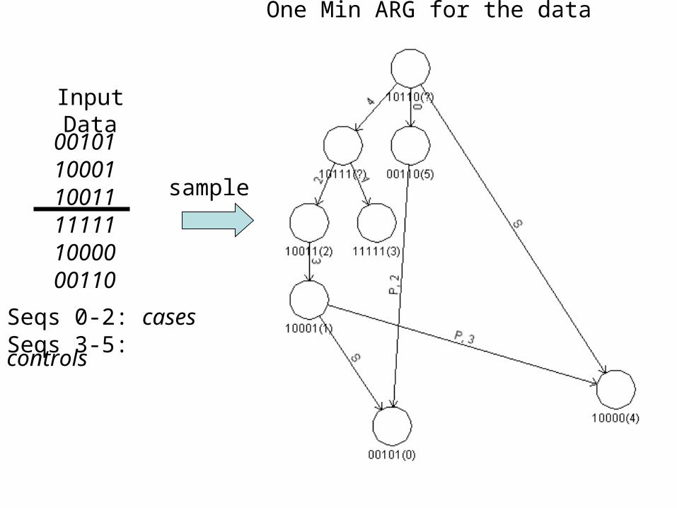
Input Data

001011000110011111111000000110

Seqs 0-2: casesSeqs 3-5: controls

sample

One Min ARG for the data

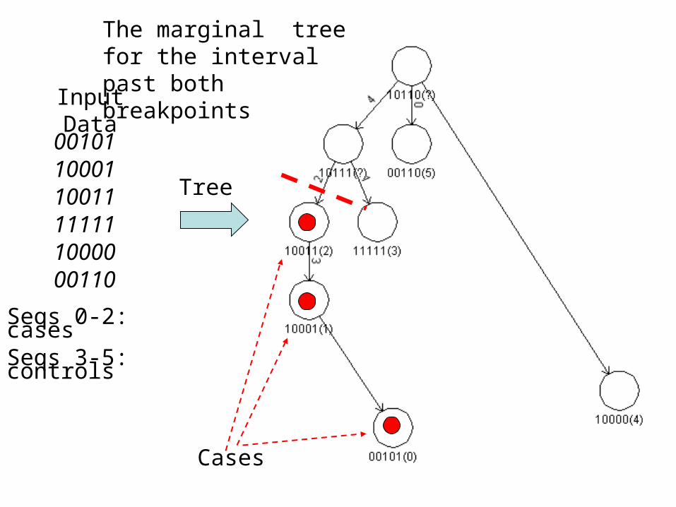
Input Data

001011000110011111111000000110

Seqs 0-2: casesSeqs 3-5: controls

Tree

The marginal tree for the interval past both breakpoints

Cases

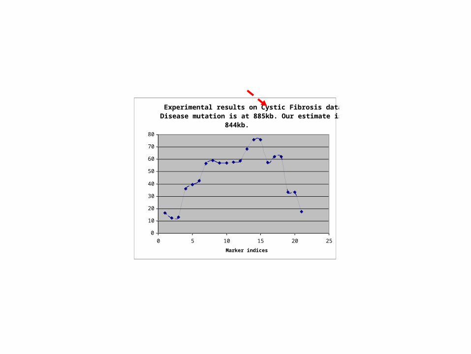
Experimental results on Cystic Fibrosis data. Disease mutation is at 885kb. Our estimate is at

844kb.

0

10

20

30

40

50

60

70

80

0 5 10 15 20 25

Marker indices

Average Chi-square value

Haplotyping (Phasing)

genotypic data using a Min ARG

Minimizing Recombinations for Genotype Data

• Haplotyping (phasing genotypic data) via a Min ARG: attractive but difficult

• We have a branch and bound algorithm that builds a Min ARG for deduced haplotypes that generate the given genotypes. Works for genotype data with a small number of sites, but a larger number of genotypes.

Application: Detecting Recombination Hotspots with

Genotype Data • Bafna and Bansel (2005) uses recombination lower

bounds to detect recombination hotspots with haplotype data.

• We apply our program on the genotype data– Compute the minimum number of recombinations for all

small windows with fixed number of SNPs– Plot a graph showing the minimum level of recombinations

normalized by physical distance– Initial results shows this approach can give good estimates

of the locations of the recombination hotspots

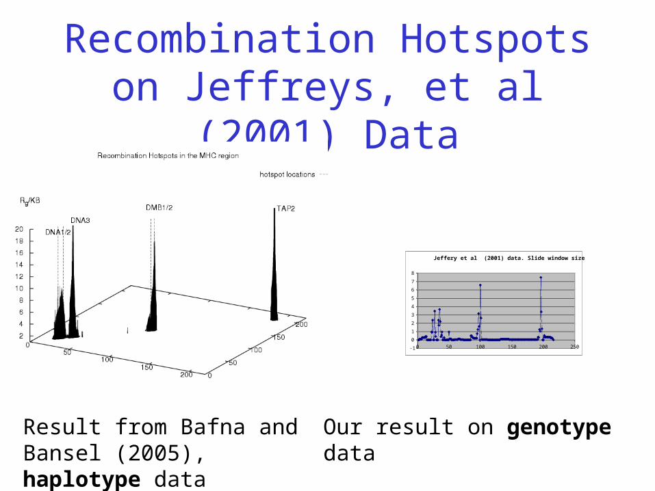
Recombination Hotspots on Jeffreys, et al (2001) Data

Jeffery et al (2001) data. Slide window size = 5

-1

0

1

2

3

4

5

6

7

8

0 50 100 150 200 250

Result from Bafna and Bansel (2005), haplotype data

Our result on genotype data

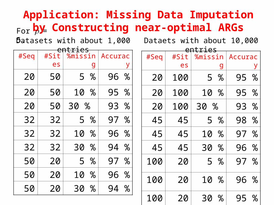
#Seq #Sites %missing Accuracy

20 50 5 % 96 %

20 50 10 % 95 %

20 50 30 % 93 %

32 32 5 % 97 %

32 32 10 % 96 %

32 32 30 % 94 %

50 20 5 % 97 %

50 20 10 % 96 %

50 20 30 % 94 %

#Seq #Sites %missing Accuracy

20 100 5 % 95 %

20 100 10 % 95 %

20 100 30 % 93 %

45 45 5 % 98 %

45 45 10 % 97 %

45 45 30 % 96 %

100 20 5 % 97 %

100 20 10 % 96 %

100 20 30 % 95 %

Datasets with about 1,000 entries Dataets with about 10,000 entries

Application: Missing Data Imputation by Constructing near-optimal ARGsFor = 5.

Haplotyping genotype data via a minimum ARG

• Compare to program PHASE, speed and accuracy: comparable for certain range of data

• Experience shows PHASE may give solutions whose recombination is close to the minimum– Example: In all solutions of PHASE for three sets of

case/control data from Steven Orzack, recombinatons are minimized.

– Simulation results: PHASE’s solution minimizes recombination in 57 of 100 data (20 rows and 5 sites).

Documents

General Constructions